Storage and selection of multiple chaotic attractors in minimal reservoir computers

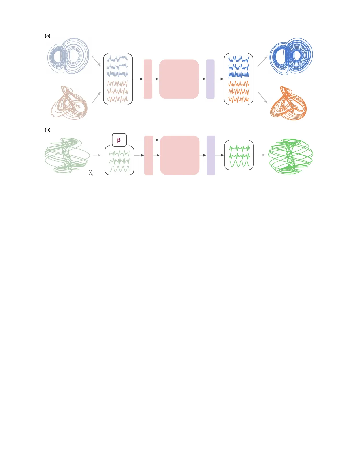
Storage and selection of multiple chaotic attractors in minimal reservoir computers Sto rage and selection of multiple chaotic attracto rs in minimal reservoir computers F rancesco Ma rtinuzzi 1 and Holger Kantz 1 Max Planck Institute for the Physics of Comple x Systems, Dresden, Germany (*Electronic mail: martinuzzi@pks.mpg.de ) (Dated: 17 March 2026) Modern predictiv e modeling increasingly calls for a single learned dynamical substrate to operate across multiple regimes. From a dynamical-systems viewpoint, this capability decomposes into the storage of multiple attractors and the selection of the appropriate attractor in response to contextual cues. In reserv oir computing (RC), multi-attractor learning has largely been pursued using large, randomly wired reservoirs, on the assumption that stochastic connectivity is required to generate sufﬁciently rich internal dynamics. At the same time, recent work shows that minimal determin- istic reservoirs can match random designs for single-system chaotic forecasting. Under which conditions can minimal topologies learn multiple chaotic attractors? In this paper , we ﬁnd that minimal architectures can successfully store multiple chaotic attractors. Howe ver , these same architectures struggle with task switching, in which the system must transition between attractors in response to external cues. W e test storage and selection on all 28 unordered system pairs formed from eight three-dimensional chaotic systems. W e do not observe a rob ust dependence of multi-attractor perfor- mance on reservoir topology . Over the ten topologies inv estigated, we ﬁnd that no single one consistently outperforms the others for either storage or cue-dependent selection. Our results suggest that while minimal substrates possess the representational capacity to model coexisting attractors, they may lack the robust temporal memory required for cued transitions. When modeling a physical phenomenon, simpler models are usually preferred because they are more tractable and interpr etable. For machine learning models, simplicity entails fewer parameters and easier training. Reservoir computing (RC) models sit naturally at this intersection: the recurrent core is ﬁxed a priori, so its structur e (and thus its behavior) can be speciﬁed and analyzed directly , and its training is linear regression. Here, we ask how simple the reservoir structure can be while still lear ning multiple chaotic attractors. Supporting multiple behav- iors splits broadly into two requir ements: storage, mean- ing that multiple attractors can be repr esented within the same substrate, and selection, meaning that an exter nal cue can reliably change the dynamics to the desired attrac- tor . W e evaluate the storage and selection of ten different minimal RC models f or learning two distinct chaotic sys- tems. W e ﬁnd that minimal deterministic reser voirs can often achieve attractor storage when trained to repr oduce multiple systems in parallel, but they typically fail at cue- driven selection in a switching task. This separation sug- gests that representing multiple chaotic patterns does not necessarily require stochastic r eservoirs, whereas reliable switching likely demands additional memory or control structure beyond the minimal designs studied here. I. INTRODUCTION Many scientiﬁc modeling problems require a single predic- tiv e model to operate across multiple dynamical regimes. For instance, weather conditions vary across geographic regions 1 , and robotic components may need to switch responses under changing e xternal stimuli 2 . In such settings, a model must store multiple distinct dynamical patterns and reliably deploy the appropriate one when conditions change. This ability can be seen as composed of two dif ferent mechanisms: stor- age , meaning that multiple stable attractors can coexist in the same system, and selection , meaning that context—or cues— reliably routes the dynamics to the desired attractor 3 . Biolog- ical brains naturally store different patterns by reusing ﬁxed neural circuitry (neural reuse, or multifunctionality) 4 , 5 . In ma- chine learning (ML), analogous capabilities are increasingly pursued via foundation models (FMs) 6 . Built to internalize families of beha viours, FMs can be steered at inference time by prompts, conditioning variables, or other context signals. For example, time-series FMs can adapt their forecasts across regimes when provided with a context window representative of novel dynamics 7 – 9 , and protein FMs can represent and gen- erate div erse structural and functional motifs within a single parameterization 10 . Data-driv en modeling of chaotic dynamics has also begun to shift toward architectures that can learn and switch between distinct attractors. T raditionally , models were trained on a sin- gle chaotic system within a ﬁxed-parameter regime to either recov er short-term trajectories or reproduce long-term statis- tical properties 11 – 16 . Howe ver , recent advances demonstrate that ML systems can generalize across different dynamical regimes. Modern approaches can, for instance, recov er tra- jectories in unseen portions of the phase space 17 , 18 , switch between dif ferent dynamical regimes in the same system 19 , and anticipate critical transitions and tipping points 20 – 22 . Fur - thermore, general-purpose time-series FMs already exhibit an emergent ability to forecast chaotic systems with no additional training 23 . Building on these results, new domain-speciﬁc FMs are no w being dev eloped speciﬁcally to generalize mul- tiple chaotic systems, enabling a single architecture to gen- erate div erse, mathematically faithful attractors at prediction time 24 , 25 . W ithin this line of research, reservoir computing (RC) has Storage and selection of multiple chaotic attractors in minimal reservoir computers 2 emerged as a particularly ﬂexible frame work. In RC, the re- current reservoir dynamics are randomly initialized and ﬁxed, while only the readout is trained with linear regression 26 , 27 . The internal reservoir can hence be treated as an e xplicit dynamical substrate whose dimensionality , connectivity , and weight structure are directly tunable. The combination of sim- ple, fast training and additional control over reservoir proper- ties mak es RC models a v aluable frame work for mechanis- tic exploration 28 : architectural and dynamical ingredients can be varied while keeping the ev olution equations consistent. Models such as echo state networks (ESNs) 29 hav e been used to model chaotic dynamics with great success 30 – 32 . Exten- sions of ESNs hav e also shown the ability to learn multiple distinct chaotic systems; by changing the training algorithm, Lu and Bassett 33 show how ESNs can switch between sys- tems, thereby showcasing dif ferent dynamical regimes. Fur- ther studies demonstrate how ESNs can retrieve chaotic sys- tems previously stored in memory 34 , and learn multistable systems 35 . Multiple dynamics can also be stored in RC sys- tems using conceptors 36 . Recent works illustrate the ability of ESNs to store multiple attractors in memory 37 , 38 . Follo w-up in vestigations have used this multistable structure to probe bi- furcations and transitions between learned attractors in reser- voir models 39 – 41 , and similar multifunctional dynamics ha ve been demonstrated in other RC architectures as well 42 – 44 . Howe ver , most RC approaches for multi-attractor learn- ing still rely on large, stochastically constructed reservoirs. The structure of the reserv oir adjacenc y matrix (also called its topology ) is known to strongly inﬂuence performance 45 – 52 . Random sparse reservoirs, the default choice in ESNs, are ex- plicitly motiv ated by the goal of producing a rich set of in- ternal dynamics 53 , which are widely regarded as essential for reservoir computation both in single 54 and multiple 34 system settings. Recent evidence, howe ver , suggests that this level of complexity is not a prerequisite for learning chaotic dynamics. Small reservoirs 48 , sparsely connected architectures 55 , and deterministic designs 56 – 58 often provide performance compa- rable to large random reservoirs. In particular , minimal deter- ministic topologies of fer more accurate and consistent results when modeling chaotic systems 59 . Is it also possible for min- imal topologies to store and recall multiple chaotic attractors? In this paper , we ev aluate whether minimal deterministic reservoir topologies can learn multiple chaotic systems in a single model. W e consider two distinct approaches: the ﬁrst is based on the blending technique (BT), in which a single ESN is trained to learn and replicate multiple systems at the same time 37 ; the second is the parameter-aw are (P A) approach, in which a single ESN can learn to switch between different learned systems in response to an external cue signal 60 . For each approach, we train a single ESN topology to learn the dy- namics of pairs of chaotic systems drawn from a pool of eight benchmark systems, yielding 28 distinct experiments per set- ting. Exploring a broad set of system pairs reduces the risk that our conclusions depend on an atypical or unlucky com- bination of systems. W e study ten simple deterministic reser- voir topologies that collecti vely cov er a broad range of designs proposed in previous work on deterministic reserv oirs 61 – 64 . A topology is considered successful if a trained ESN can ac- curately reproduce both chaotic attractors associated with a giv en system pair . Under the BT protocol, success means that the ESN simultaneously generates faithful forecasts for both systems from the state input. Under the P A protocol, suc- cess requires cue-dependent selection of different dynamics. In our experiments, minimal deterministic topologies consis- tently achiev e attractor storage in the BT setting, but they do not support robust cue-dependent selection in the P A setting. The structure of the paper is as follows. In Sec II we detail the technical aspects of the work, starting from a description of ESNs and their minimal topologies in Sec. II A , and how to train them to learn multiple systems in Sec. II B . Further sections detail the metric used to quantify the v alidity of the results in Sec. II C and the systems and preprocessing used in the study in Sec. II D . W e present the results in Sec. III . Section IV pro vides a ﬁnal summary and discussion of the work. I I. METHODS A. Minimal Reservoir Computers RC refers to a f amily of ML models that uses dynamical systems for computation 26 , 27 . The shared component of RC architectures is the reservoir , a high-dimensional dynamical system. The role of the reservoir is to provide a nonlinear expansion of the data, exposing linear dependencies. Model- ing with an RC in volv es three main stages: (i) the data is ﬁrst passed through the RC model. (ii) Afterwards, the resulting reservoir states are used for training against the desired tar- get data. Linear regression is usually used for training in RC models 65 . Finally (iii), the model can be used for the chosen task. An y ML task, such as regression, forecasting, or classi- ﬁcation, can be done with a reservoir computer . Amongst RC models, echo state networks (ESNs) 29 hav e long been studied in the ﬁeld of nonlinear dynamics due to their simple construction and fast training. Stemming from the ML literature, ESNs use a recurrent neural network (RNN) as the reservoir . Unlike traditional RNNs, which are trained via backpropagation, ESNs’ internal weights are randomly initial- ized and held ﬁxed. Only the last layer is trained, using linear regression. Formally , let u ( t ) ∈ R D in be the input vector at time t, then the time evolution of the ESN is represented by x ( t ) = ( 1 − α ) x ( t ) + α tanh ( W in u ( t ) + Wx ( t − 1 ) + b ) , (1) where x ( t ) ∈ R D res is the reservoir state at time t , and α is the leaky coefﬁcient, which controls the timescales of the e volu- tion of the ESN. The matrix W in ∈ R D res × D in denotes the in- put matrix, while W ∈ R D res × D res is usually referred to as the r eservoir matrix. The term b ∈ R D res adds a bias component, useful to break internal simmetries . Because of the random and static nature of ESN matrices, their initialization plays an important role. In traditional ESN literature, the input and reservoir matrices are initialized ran- domly , with various hyperparameters controlling their over - all behavior . General guidelines dictate that the input matrix Storage and selection of multiple chaotic attractors in minimal reservoir computers 3 DL SLFB DLFB SLDB SC SLFC CJ FC SLC DC (a) (f) (b) (g) (c) (h) (d) (i) (e) (j) FIG. 1. Minimal deterministic reservoir topologies. Each panel sho ws the nonzero entries (magenta) of the 10 × 10 reservoir matrix W . All the nonzero weights have the same magnitude and sign. Zero entries are shown in light gray . Panels correspond to the following structures: (a) delay line (DL), (b) delay line with feedback connections (DLFB), (c) simple cycle (SC), (d) cycle with jumps (CJ), (e) self-loop cycle (SLC), (f) self-loop feedback cycle (SLFB), (g) self-loop delay line with backward connections (SLDB), (h) self-loop with forward connections (SLFC), (i) forward connections (FC), and (j) double cycle (DC). be randomly generated with weights drawn from U ( − σ , σ ) , where σ controls the nonlinearity that is applied to the input, and is subsequently treated as a hyperparameter . The reser- voir matrix requires greater care, as it is the primary driv er of the ESN’ s dynamics. This matrix is generally generated as sparse with sparsity θ , following a Erd ˝ os–Rényi connection graph. After being generated, the matrix W ∗ is then scaled to a chosen spectral radius ρ to obtain the ﬁnal reservoir matrix W . It follows that ρ and θ are considered hyperparameters to be tuned. More speciﬁcally , the spectral radius plays an im- portant, and still hotly debated, role in the performance of the ESN 66 – 68 . T o reduce this complexity and assess whether it is nec- essary in the ﬁrst place, recent approaches have used sim- pler setups for building ESNs. First proposed by Rodan and T ino 61 , minimum-complexity ESNs (MESNs) offer a simple approach to ESN construction. The rules follow simple steps: (i) all the weights used are the same, with their magnitude set and not randomly deﬁned. (ii) The topologies of the reservoirs are also set and not random. (iii) the signs of the reservoir weights are the same, while the signs of the weights of the input layer do change. Follo wing these rules, multiple alter- nativ e topologies hav e been proposed 62 – 64 . In this work, we consider the following topologies: • Delay line (DL) 61 , composed only of weights arranged in a line. The nonzero entries of the matrix are located on the lower subdiagonal W ( i + 1 , i ) = r , i ∈ [ 1 , D res − 1 ] . • Delay line with feedback connections (DLFB) 61 , which shares the same structure as DL, with the ad- dition of feedback weights. The matrix is built with nonzero weights on the lower subdiagonal W ( i + 1 , i ) = r and on the upper subdiagonal W ( i , i + 1 ) = b where i ∈ [ 1 , D res − 1 ] . • Simple cycle (SC) 61 , where the weights form a cy- cle. The SC matrix has nonzero elements on the lo wer subdiagonal W ( i + 1 , i ) = r , i ∈ [ 1 , D res − 1 ] , with the ad- dition of a weight located in the upper right corner W ( 1 , D res ) = r • Cycle with jumps (CJ) 62 , builds on SC, but adds bidi- rectional jump connections of ﬁxed distance ℓ , all with weight r j . Nonzero elements of CJ are on the lower subdiagonal W ( i + 1 , i ) = r , i ∈ [ 1 , D res − 1 ] , and the up- per right corner W ( 1 , D res ) = r , following SC. Addi- tionally , jump entries r j are added, with a jump size 1 < ℓ < ⌊ D res / 2 ⌋ . If ( D res mod ℓ ) = 0, there are D res /ℓ jumps. The ﬁrst jump starts from the ﬁrst weight in the cycle, and connects it to 1 + ℓ . The last jump is from unit D res + 1 − ℓ to the ﬁrst one. If ( D res mod ℓ )  = 0, there are ⌊ D res /ℓ ⌋ jumps, the last ending in unit D res + 1 − ( D res mod ℓ ) . The jumps are bidirectional and share the same connection weight r j . • Self-loop cycle (SLC) 63 , also builds on the SC with the addition of self-loops. Nonzero weights are W ( i + 1 , i ) = r , i ∈ [ 1 , D res − 1 ] , W ( 1 , D res ) = r , and W ( i , i ) = l l , i ∈ [ 1 , D res ] • Self-loop feedback cycle (SLFB) 63 , continues to build on the cycle reservoir , with the addition of self-loops and feedbacks. Similarly to the SC, nonzero weights are Storage and selection of multiple chaotic attractors in minimal reservoir computers 4 W ( i + 1 , i ) = r , i ∈ [ 1 , D res − 1 ] , W ( 1 , D res ) = r . Additionally , if i is odd W ( i , i ) = l l , i ∈ [ 1 , D res ] , otherwise W ( i , i + 1 ) = r , i ∈ [ 1 , D res − 1 ] . • Self-loop delay line with backward connections (SLDB) 63 , extends the delay-line by adding self-loops on ev ery unit and backward links to the second pre vi- ous unit. Nonzero entries are W ( i , i ) = l l for i ∈ [ 1 , D res ] (self-loops), W ( i + 1 , i ) = r for i ∈ [ 1 , D res − 1 ] (forw ard path), and W ( i , i + 2 ) = r for i ∈ [ 1 , D res − 2 ] (backward connections to the second previous unit). • Self-loop with forward connections (SLFC) 63 , re- mov es the standard forward path and keeps only con- nections of length two, forming two disjoint forward chains over odd and even indices, plus self-loops on ev ery unit. The nonzero entries are W ( i , i ) = l l for i ∈ [ 1 , D res ] and W ( i + 2 , i ) = r for i ∈ [ 1 , D res − 2 ] . • Forward connections (FC) 63 , identical to SLFC but without self-loops. The only nonzero entries are W ( i + 2 , i ) = r for i ∈ [ 1 , D res − 2 ] . • Double cycle (DC) 64 , again builds on SC, but it adds an additional cycle in the opposite direction. The nonzero elements are then W ( i + 1 , i ) = r , i ∈ [ 1 , D res − 1 ] and W ( 1 , D res ) = r as in SC, plus other cycle W ( i , i + 1 ) = r , i ∈ [ 1 , D res − 1 ] and W ( D res , 1 ) = r T o further minimize the number of free parameters in these initializers, we set r = l l = r j = 0 . 1 in this work. a. T raining Gi ven an input sequence { u ( t ) } T 0 , we drive the reservoir using Eq. 1 . Follo wing standard procedures, we remov e an initial transient period τ = 300 from the train- ing states, resulting in a set of states { x ( t ) } T τ . Each state x ( t ) is subsequently transformed with a function such that h ( t ) = H ( x ( t )) = [ x ( t ) ; x 2 ( t )] , where [ ; ] indicates vertical con- catenation. The resulting states are collected into a states ma- trix H , where each column corresponds to one time step. W e like wise collect the desired outputs into a target matrix Y target . T raining then consists of ﬁtting a linear readout W out that maps reservoir states to targets. W e estimate W out via ridge regression by minimizing L ( W out ) =   Y target − W out H   2 2 + λ ∥ W out ∥ 2 2 . (2) The minimizer of Eq. 2 admits the closed-form solution W out = Y target H ⊤  HH ⊤ + λ I  − 1 , (3) where I is the identity matrix, and λ is the regularization co- efﬁcient controlling the strength of the ℓ 2 penalty . b . F or ecasting After estimating W out , we run the ESN in forecasting mode by computing the output v ( t ) = W out h ( t ) , (4) where v ( t ) denotes the ESN output at time t . Throughout this work, we e valuate models in an autoregressi ve (closed-loop) forecasting regime. During training, the target sequence is chosen one step ahead of the input, i.e., y target ( t ) = u ( t + 1 ) , so that the trained readout approximates the one-step map ˆ u ( t + 1 ) = v ( t ) . At prediction time, the ESN is run autonomously by feeding this estimate back as the next input and iterating for T steps. Under this closed-loop rollout, Eq. ( 1 ) becomes x ( t ) = ( 1 − α ) x ( t ) + α tanh ( W in W out x ( t − 1 ) + Wx ( t − 1 ) + b ) , (5) B. Proto cols for multi-attracto r lea rning Since standard ESNs are trained for a single input–output mapping, the setup of Sec. II A does not, by itself, address the multi-attractor setting studied here. While there exist dif fer- ent ways to learn multiple dynamics in a reservoir computing context (see the relev ant paragraph in Sec I ), in this work we limit our exploration to two distinct methods. Speciﬁcally , we consider (a) the blending technique (BT ; Sec. II B 1 ), which probes attractor storag e by training on concatenated trajecto- ries, and (b) the parameter-aw are (P A; Sec. II B 2 ) protocol, which tests cue-dependent selection by injecting a label sig- nal that is intended to route the dynamics toward a chosen attractor . Before passing the attractors to the ESNs, we sep- arate them in phase space. Each attractors’ states are shifted by a v alue η = 0 . 2. In our case of two distinct attractors, the coordinates are shifted as follows: ( x + η , y + η , z + η ) , ( x − η , y − η , z − η ) . 1. Blending T echnique Proposed by Flynn, Tsachouridis, and Amann 37 , in the BT approach, the ESN is fed with a concatenation of the ev olution vectors of two attractors χ i , i ∈ { 1 , 2 } . Let u χ 1 ( t ) ∈ R D in , 1 be the coordinates of the points of attractor χ 1 , and u χ 2 ( t ) ∈ R D in , 2 be the coordinates of the points of attractor χ 2 . The ESN input vector is then u bt ( t ) =  u χ 1 ( t ) u χ 2 ( t )  , (6) where u bt ( t ) ∈ R D in , 1 + D in , 2 . In the context of this work we use D in , 1 = D in , 2 = 3. Figure 2 a shows a schematic representation of how an RC is trained in the BT technique. W e note that, in the original paper, an additional parameter β ∈ [ 0 , 1 ] controls the blending (hence the naming), u bt ( t ) =  β u χ 1 ( t ) ( 1 − β ) u χ 2 ( t )  , (7) providing a bifurcation parameter for the multifunctional ESN. In this work, we use concatenation without the blending parameter to focus strictly on determining whether minimal ESNs can store multiple attractors. Remo ving the blending parameter does not impact the performance of the models, as it is implied by Fig. 7a of Ref. 37 . Storage and selection of multiple chaotic attractors in minimal reservoir computers 5 (a) (b) χ i β i FIG. 2. Appr oaches for multi-attractor learning in reser voir computing. P anel (a) shows the approach for attractor storage in an echo state network (ESN) using the blending technique (BT). T wo chaotic trajectories are provided in parallel by concatenating their state vectors into a single input, u bt ( t ) = [ u χ 1 ( t ) ; u χ 2 ( t )] . This joint input drives the ESN, and a single linear readout is trained to produce a concatenated output trajectory that reconstructs both systems simultaneously (right time series and attractors; colors distinguish the two systems). Panel (b) illustrates cue-dependent selection using the parameter-aware (P A) approach. In addition to the state input, a scalar cue β i identifying the target attractor is injected through the bias term in Eq. ( 8 ). The ESN is then run with β i held ﬁxed so that the autonomous dynamics are expected to con verge to, and reproduce, the attractor associated with that cue. In both panels, the light pink boxes indicate untrained matrices, while the light violet box indicates the trained readout. 2. P arameter A wa re T echnique Similarly to OHagan, Keane, and Flynn 41 , we imple- ment a simpliﬁed version of the P A technique for training ESNs 20 , 21 , 34 . In this technique, each attractor is identiﬁed by assigning it a unique scalar label. The attractor label is then fed into the ESN via a parameter-dependent bias term in the state update to recov er the associated dynamics. Formally , let β i ∈ R , i ∈ { 1 , . . . , m } , be the scalar label for each of the m systems. The parameter-a ware ESN is then de- ﬁned as x ( t ) = ( 1 − α ) x ( t − 1 ) + α tanh  W in u β i ( t ) + Wx ( t − 1 ) + β i b  . (8) where u ( t ) is the input at time t and β i is kept ﬁxed for all sam- ples belonging to attractor i . W e depict the labeling scheme of P A in Fig. 2 . While the ﬁgure shows the RC being trained with a single system, the method supports storing multiple at- tractors, each with its own label. The difference in the values of β i between attractors is gov- erned by the hyperparameter δ β , which controls the spacing between labels via β i = β i − 1 + δ β . Follo wing preliminary hyperparameter selection, we choose δ β = 0 . 4, starting from β 1 = 0 . 1 for the ﬁrst attractor . T raining follows the standard ESN procedure, with the ad- dition that the label β i is provided alongside each training sample and enters the state update through the bias term in Eq. ( 8 ). Concretely , for each system i ∈ { 1 , . . . , m } we gener- ate a training trajectory { u i ( t ) } T t = 1 and associate ev ery sample in that trajectory with the constant label β i . W e then con- struct a single training sequence by concatenating these la- beled trajectories in time. During this concatenated teacher- forced pass, the input u ( t ) is the current true state from the ac- tiv e system segment and the label is set to the corresponding value β ( t ) = β i for that entire segment; when the sequence transitions to the next system segment, the label is switched accordingly . Reservoir states are collected from this full la- beled sequence and a single readout W out is trained by ridge regression as in the standard ESN. During autoregressi ve forecasting, we select the target sys- tem by ﬁxing the label to β ( t ) ≡ β i for all prediction steps and initializing the ESN with suitable initial conditions. The network is then run in closed loop: at each step the predicted output ˆ u ( t + 1 ) is fed back as the next input, yielding the au- tonomous update in Eq. ( 5 ) with the bias term scaled by the chosen label β i . The accuracy of the forecast is assessed by ev aluating all reproduced attractors individually , and then re- porting the av erage score. Storage and selection of multiple chaotic attractors in minimal reservoir computers 6 log dKLD = 0.043 log KLD = 0.043 (a) log dKLD = 0.418 log KLD = 0.418 (b) log dKLD = 0.644 log KLD = 1.3 (c) log dKLD = 0.878 log KLD = 2.092 (d) log dKLD = 0.486 log KLD = 3.24 (e) FIG. 3. Effect of prediction deterioration on metric changes. In this ﬁgure, we provide Lorenz attractor overlays, illustrating how recon- struction quality maps to the discrete state–space Kullback–Leibler diver gence (KLD). Grey curves show the reference Lorenz trajectory . In panel (a), the comparison trajectory (pink) is generated by the same Lorenz equations but using different initial conditions; both the standard discrete KLD (dKLD) and the penalized v ariant (KLD) remain small. Panels (b–e) show progressiv ely degraded ESN forecasts (violet). As prediction quality deteriorates and forecasted trajectories increasingly deviate from the true state space, the standard dKLD exhibits relatively low sensitivity . On the other hand, the penalized KLD increases with the degree of prediction failure, providing a clearer indication of recon- struction failure. Metric values reported below each panel are in log 10 scale. C. A ccuracy metric - Kullback-Leibler divergence As a measure of model performance, we use the Kullback- Leibler diver gence (KLD) deﬁned across space, in line with previous works 69 – 72 . The chosen metric ensures that the pre- dicted attractor aligns geometrically with the true attractor . Follo wing Hemmer and Durstewitz 24 we discretize the D in = 3-dimensional state space into K = m N bins using m = 30 bins per dimension. Let ˆ p true i and ˆ p RC i denote the normalized oc- cupancy frequencies of bin i estimated from the ground-truth trajectory and from the reservoir -generated trajectory , respec- tiv ely . The dKLD of a giv en RC per model is then approxi- mated as dKLD ≈ K ∑ i = 1 ˆ p true i log  ˆ p true i ˆ p RC i  . (9) Howe ver , the metric in Eq. 9 only compares occupancy prob- abilities on the ﬁnite grid deﬁned over the region spanned by the true attractor . In practice, reservoir predictions may drift outside this reference domain. The corresponding excursions would then not be reﬂected by the histogram-based dKLD. T o account for catastrophic failures, we augment the div ergence with an out-of-bounds (OOB) penalty . Concretely , we deﬁne an axis-aligned bounding box from the true trajectory by set- ting, for each state-space dimension d , lower and upper lim- its ℓ d = min ( x true d ) − 0 . 1 σ true d and h d = max ( x true d ) + 0 . 1 σ true d , where σ true d is the standard deviation of the true coordinates along dimension d . W e then compute the maximum relati ve violation of the predicted trajectory with respect to this box, v = max d max  0 , ℓ d − min ( x pred d )  + max  0 , max ( x pred d ) − h d  h d − ℓ d , (10) and, whenev er v > 0, we return a penalty value KLD = w OOB v , (11) with weight w OOB = 10 2 . Otherwise ( v = 0), we proceed with the histogram-based dKLD computation on the binning in- duced by [ ℓ d , h d ] . The modiﬁed KLD ensures that predictions that leave the support of the true attractor are explicitly penal- ized. The resulting KLD values will also appear much larger than those reported in similar works. Figure 3 illustrates the difference between the tw o metrics for varying lev els of at- tractor reconstruction quality . It is possible to observe that the KLD with OOD penalty returns results that are consistent with the visible deterioration in the attractor reconstruction by the ESN. D. Chaotic systems and data generation W e consider eight dif ferent chaotic systems taken from dysts 73 . From this set, we form all unique combinations of two distinct systems. This yields  8 2  = 28 unique two-system combinations, which we refer to as system pairs. Each combi- nation deﬁnes the systems that the minimal reservoir comput- ers are tasked to reproduce. W e provide the list of the systems used (with respectiv e equations, parameters, and inte gration steps) in Appendix A . Each system trajectory is normalized to hav e a mean of zero and a standard deviation of 1 74 . For the numerical integration, we sourced the system deﬁnitions from the Julia port of dysts , ChaoticDynamicalSystemLibrary.jl 75 . W e use the Feagin12 solver from the DifferentialEquations.jl package 76 , with absolute and relative tolerances set to 10 − 13 , to integrate the systems. Each system has its own integration step size, as deﬁned in dysts . For each system, we collect 7000 data points for training, 3000 data points for validation, and 2500 for testing. The ﬁrst 300 data points are discarded to account for transient dynam- ics. The validation points are used for hyperparameter tun- ing. Each ESN undergoes a grid search to ﬁnd the optimal Storage and selection of multiple chaotic attractors in minimal reservoir computers 7 log KLD 0.0 2.5 5.0 7.5 CJ FC SLDB DL DC DLFB SLFC SC SLFB SLC log KLD 0.0 2.5 5.0 7.5 (a) (b) (c) FIG. 4. Multi-attractor learning accuracy across minimal reservoir topologies . Panel (a) shows the results of the blending technique (BT). The violin plots indicate the distributions of log 10 Kullback-Leibler diver gence (KLD) over all 28 unordered system pairs for each reservoir topology (ordered by increasing median). Panel (b) illustrates the results for the parameter-aw are (P A) approach. The panel maintains the same topology ordering and visualization used in BT . In both panels, violins show the distribution across system pairs, and the black dot marks the median log 10 KLD for that topology; the apparent extension below zero is due to violin smoothing and does not imply negati ve KLD values. (c) Representativ e system pair reconstruction example for LorenzSprottS using the self-loop delay line with backward connections (SLDB) topology in the BT setting. Dashed curves show the reference attractors and solid curves the ESN-generated attractors, with different colors distinguishing the two systems. The accuracy for the system pair corresponds to log 10 KLD = 0 . 692. value of the ridge regression parameter and leaky coefﬁcient. The hypergrid is determined by latin hypercube sampling 77 , 78 with boundary values of [ 0 . 1 , 1 . 0 ] for the leaky coefﬁcient, and [ 10 − 12 , 10 − 1 ] for the ridge regression parameter . For training, we provide the MESNs with 10 trajectories per system, each starting from a dif ferent location on the attractor . The ini- tial conditions provided in dysts are used to generate the ﬁrst trajectory . Subsequent trajectories are obtained by shifting the same underlying trajectory by 50 time steps, so that each tra- jectory begins at a different position on the attractor . I I I. RESUL TS In this section we detail the results obtained in this work. T o perform the simulations, we used the Julia pro- gramming language 79 . For the integration of the chaotic systems, we relied on OrdinaryDiffEq.jl 76 , while for the visualization we used CairoMakie.jl 80 . All the dif- ferent reservoir topologies and the implementation, train- ing, and forecasting of the ESNs are sourced through ReservoirComputing.jl 81 . For each system pair and topology , we run ten simulations, each starting from a dif- ferent initial condition. A. Sto rage vs Selection Across Minimal Deterministic Reservoir T op ologies Figure 4 summarizes the ov erall performance of the differ- ent minimal deterministic reservoir topologies in reproducing multiple chaotic dynamics when trained under the two ap- proaches considered in this study . Performance is reported on a logarithmic scale to accommodate the wide range of ob- served values. The reported value for the system pair is taken as the average of the two KLDs obtained for each system. The ﬁgure aggregates results over all 28 unordered pairs of chaotic systems. In addition to the aggregate error statistics, the ﬁgure includes a representativ e phase-space visualization showing a case in which a single trained model successfully reconstructs both members of a system pair . In Fig. 4 a, we report the distribution of log 10 KLD values obtained in the BT task for each minimal topology . Each light-blue violin corresponds to one topology (CJ, FC, SLDB, DL, DC, DLFB, SLFC, SC, SLFB, SLC; ordered left-to-right by increasing median log 10 KLD) and summarizes the v ari- ability of errors across all 28 system pairs. The vertical axis extends down to approximately − 2 . 5; this lo wer range is due to the kernel-density smoothing used to draw the vio- lins and does not indicate negativ e KLD v alues. The black dot marks the median log 10 KLD for each topology . Under this ordering, the best-performing topology is CJ, with median log 10 KLD = 2 . 866 and an interquartile range of [ 1 . 050 , 3 . 543 ] in log 10 KLD. On the other side, the worst performing topol- ogy is SLC, with median log 10 KLD = 3 . 357 and an interquar- Storage and selection of multiple chaotic attractors in minimal reservoir computers 8 Reservoir initializer SLC SLFB SC SLFC DLFB DC DL SLDB FC CJ System pair Ai-Ar Ai-C Ai-G Ai-H Ai-L Ai-R Ai-S Ar-C Ar-G Ar-H Ar-L Ar-R Ar-S C-G C-H C-L C-R C-S G-H G-L G-R G-S H-L H-R H-S L-R L-S R-S Reservoir initializer SLC SLFB SC SLFC DLFB DC DL SLDB FC CJ log KLD 2 4 6 (a) (b) FIG. 5. Perf ormance of minimal reservoirs across multi-attractor learning tasks and system pairs . (a) Heat map of prediction qual- ity for each combination of reservoir initializer and chaotic system pair under the blending technique (BT) approach, quantiﬁed as the log 10 of the mean KLD over runs. Panel (b) reports the same results as Panel (a), but for the parameter -aware (P A) training scheme. In both panels, darker tiles indicate lower error (better forecasts), indi- cating how individual minimal initializers generalize across different blended systems and how their performance patterns change between training schemes. tile range of [ 1 . 095 , 3 . 941 ] . V iolin width encodes the rel- ativ e density of outcomes at a giv en error value. W e note that, across all topologies, the distrib utions are consistently bimodal in log space: using the KDE-based split, the av erage separation threshold is ⟨ log 10 KLD ⟩ ≈ 1 . 966 (std. 0.137), and the resulting lobe means averaged over initializers are ⟨ µ 1 ⟩ = 0 . 970 ± 0 . 064 and ⟨ µ 2 ⟩ = 3 . 642 ± 0 . 133 in log 10 KLD. More speciﬁcally , for CJ the a KDE-based split at log 10 KLD ≈ 1 . 973 separates a lo wer-error lobe with mean log 10 KLD = 0 . 929 from a higher-error lobe with mean log 10 KLD = 3 . 617, while for SLC a KDE-based split at log 10 KLD ≈ 2 . 054 sepa- rates a lower-error lobe with mean log 10 KLD = 1 . 003 from a higher-error lobe with mean log 10 KLD = 3 . 799. In Fig. 4 b, we report the distribution of log 10 KLD val- ues obtained in the parameter-a ware (P A) task for each mini- mal topology . W e keep the topology ordering and visual en- coding as in Fig. 4 . Each violin plot aggregates outcomes across all 28 system pairs, with the black dot indicating the median log 10 KLD for the corresponding topology . Relati ve to the BT setting, the P A distributions are concentrated in a narrower range, with medians spanning from 2 . 466 (CJ) to 3 . 098 (DLFB), and interquartile ranges that largely over - lap across topologies. Under this ordering, the lowest me- dian is again obtained by CJ (median log 10 KLD = 2 . 466, IQR [ 2 . 241 , 2 . 885 ] ), while the highest median is observed for DLFB (median log 10 KLD = 3 . 098, IQR [ 2 . 500 , 3 . 494 ] ). Un- like the BT results, the violin shapes do not exhibit a consis- tent shared structure across initializers; instead, the densities vary between topologies and system pairs, reﬂecting hetero- geneous outcomes in the P A setting. Finally , we provide a representati ve phase-space exam- ple from the BT experiments in Fig. 4 c. The panel sho ws a successful two-attractor reconstruction for the Lorenz and SprottS systems using the SLDB topology . The two sys- tems are shown with distinct colors, and for each system, the reference trajectory is plotted with a dashed line while the corresponding ESN-generated trajectory is plotted with a solid line. The example sho wn corresponds to a case with log 10 KLD = 0 . 692 (i.e., KLD ≈ 4 . 92) for the LorenzSprottS pair under SLDB. Figure 5 pro vides a more detailed vie w of reconstruction accuracy across the different minimal reservoir topologies by showing the results for the individual system pairs. For each pair of chaotic systems and each reservoir initializer/topology , we report the mean KLD from that experiment, averaged over 10 initial conditions for both systems. Darker colors indicate smaller mean diver gences, and thus higher accuracy , while brighter colors indicate larger mean diver gences. System pairs are labeled using the ﬁrst letter of each system name, follow- ing the nomenclature deﬁned in Appendix A . For instance, the LorenzSprottS pairing is identiﬁed as L-S. W e show the mean KLD heat map for the BT setting in Fig. 5 a. In the panel, each cell represents the mean of 10 runs from a single BT experiment, deﬁned by a speciﬁc system pair and a speciﬁc reservoir initializer . W e observ e pronounced horizontal patterns: for many system pairs, the mean error re- mains consistently low or consistently high across virtually all in vestigated topologies. More speciﬁcally , we see that the lowest-error rows with consistent performances are AiR, with ⟨ log 10 KLD ⟩ = 0 . 934, ArR with ⟨ log 10 KLD ⟩ = 0 . 970, and RS with ⟨ log 10 KLD ⟩ = 0 . 979; ArC also displays uniformly low log 10 KLD v alues across columns (ro w mean 1 . 050). Con- versely , the CH row consistently yields the highest error, with ⟨ log 10 KLD ⟩ = 6 . 261. Follo wing, HL is the next-highest row with ⟨ log 10 KLD ⟩ = 5 . 424, again showing clear consistenc y across reservoir designs. In contrast, we ﬁnd little to no column-wise structure. In fact, no single initializer performs consistently for the majority of system pairs. The CJ topology reports the highest number of successfully reproduced sys- tem pairs, consistent with its better performance reported in Fig. 4 a. Overall, no discernible pattern is evident in the spe- ciﬁc behavior of the topologies. Storage and selection of multiple chaotic attractors in minimal reservoir computers 9 Multifunctionality score 0.2 0.0 0.2 Reservoir initializer SLC DC DL SC SLFC DLFB FC SLDB CJ SLFB FIG. 6. Overall multifunctionality ranking of minimal reser voirs . Multifunctionality score for each reservoir initializer, deﬁned as the difference between the fraction of blended system pairs where the initializer ranks in the top three and the fraction where it ranks in the bottom three (higher is better). Points show the score per ini- tializer , with horizontal lines indicating the distance to zero (vertical dashed line). Initializers at the top with positiv e scores (e.g., SLFB, CJ, SLDB) are both frequently among the best and rarely among the worst across tasks, while those with negati ve scores (e.g., SLC) tend to perform poorly more often than well. In contrast to panel Fig. 5 a, we do not ﬁnd comparably strong structures in Fig. 5 b, where we report the analogous log 10 mean KLD heat map for the P A setting. In this con- text, the heat map appears more homogeneous, with moderate variation across rows and columns. W e observe a single hor- izontal line corresponding to the HR pair , which yields the highest errors, with ⟨ log 10 KLD ⟩ = 3 . 235. The wide range of behaviours underlines the results illustrated in Fig. 4 b, where the P A results also lacked structure compared to the BT coun- terpart. B. The role of reservoir top ology and system complexity In this Section, we want to further in vestigate the main driv ers of ESN performance in our setting. More speciﬁcally , we differentiate between: (i) intrinsic differences in the dif- ﬁculty of the target system pairs, and (ii) performance differ- ences attrib utable to reservoir topology . This question arises from the desire to in vestigate whether certain initializers are broadly ef fectiv e across many pairings, or if a subset of sys- tem pairs is systematically easier to reproduce regardless of the reservoir design. As we can observe from Fig. 4 a and Fig. 5 a, the BT setting provides the optimal conditions to in- vestigate this direction. Additionally , the BT approach pro- vides valid reconstructions of the system pairs, whereas P A does not. The P A setting also yields largely overlapping error distributions and weak pairtopology structure in our minimal regime (Figs. 4 b and 5 b). It would then be difﬁcult to separate topology- versus system-dri ven effects. Therefore, we use BT as the primary basis for the topology-versus-system analysis in the present section. Figure 6 summarizes an overall ranking of the minimal reservoir initializers using a single multifunctionality score computed from the BT experiments. For each initializer (listed on the vertical axis), the score on the horizontal axis is deﬁned as the difference between (i) the fraction of sys- tem pairs for which that initializer ranks among the top three performers and (ii) the fraction for which it ranks among the bottom three. It follo ws that larger values indicate more fre- quent high rankings and fe wer lo w rankings. Under this def- inition, we see that SLFB obtains the highest score (0.214), appearing in the top three for 10 of the 28 system pairs and in the bottom three for 4 of the 28 pairs. SLDB and CJ follo w with identical scores of 0.143; both initializers appear in the top three around 39% of the time and in the bottom three for 7/28 pairs. At the opposite end, SLC shows the most negati ve score, − 0 . 357, e ven though it ranks in the top three for 6/28 pairs and in the bottom three for 16 pairs. The remaining ini- tializers cluster closer to zero. For instance, FC has a small positiv e score of 0.071, whereas DC (-0.107) and DL (-0.071) lie on the negativ e side of the zero reference. Figure 7 provides an o vervie w of BT performance at the lev el of individual chaotic systems. W e aggregate results across all pairs of blended systems that include a gi ven sys- tem, summarizing how each attractor contrib utes to perfor- mance across the set of pairwise tasks. The ﬁgure reports two complementary summaries: a rank-based statistic, which measures ho w frequently each system appears among the best- performing pairs for a given initializer , and an error-based statistic, which reports for each systeminitializer combination the log 10 of the mean KLD averaged ov er all pairs that include that system. In Fig. 7 a, we show the rank-based metric. For each ini- tializer , we rank all 28 system pairs by their mean KLD and select the best K=5 pairs. W e then count how man y times each system appears within these ﬁv e pairs and di vide by 2K=10, since the top-K list contains K pairs and therefore 2K system occurrences in total. Thus, a tile value of 0.40 means that the corresponding system appears 4 times among the 10 system occurrences present in the top-5 pairs (the maximum possible is 0.50, i.e., 5 out of 10, because a system can appear in at most 5 distinct pairs). W e ﬁnd that Rössler is the most frequently represented system across initializers, attaining a value of 0.40 for SLFB, DC, and FC, and 0.30 for several others (e.g., SLC, SC, SLFC, DL, CJ). SprottS is also among the top 5 multi- ple times, achieving 0.30 for SC, SLFC, DLFB, DL, SLDB, and CJ. In contrast, sev eral systems appear only sporadically in the top-5 sets: amongst the worst performers, Lorenz and Halvorsen reach at most 0.10 (e.g., Lorenz: DLFB/SLDB/FC; Halvorsen: DL/SLDB/FC), and Chua appears at most 0.10 (SLFB or DLFB), with some initializers sho wing 0.00 for that row . Storage and selection of multiple chaotic attractors in minimal reservoir computers 10 Aizawa Arneodo Chua GenesioTesi Halvorsen Lorenz Rossler SprottS Fraction in top-5 pairs 0.0 0.1 0.2 0.3 0.4 Reservoir initializer SLC SLFB SC SLFC DLFB DC DL SLDB FC CJ Aizawa Arneodo Chua GenesioTesi Halvorsen Lorenz Rossler SprottS log ₁₀ KLD 2 3 4 5 (a) (b) FIG. 7. Systemspeciﬁc perf ormance of minimal reservoirs . (a) Fraction of times each chaotic system appears in the top-5 best per- forming blended pairs for a giv en initializer (columns). Darker colors indicate that the corresponding initializer tends to perform especially well on tasks inv olving that system. (b) Mean prediction quality for each systeminitializer combination, measured as the log 10 of the av- erage Kullback-Leibler di vergence (KLD) ov er all blended pairs that contain that system. Lo wer values (clearer tiles) correspond to bet- ter performance. Rows correspond to individual chaotic systems and columns to the minimal reservoir initializers (abbreviations as in the main text). In Fig. 7 b, we report the error-based statistic. For each sys- teminitializer combination, we compute the mean KLD a v- eraged o ver all blended pairs that contain the giv en system (sev en pairs per system) and display its log 10 value. The re- sulting patterns are consistent with the rank-based metric of Fig. 7 a: systems that appear frequently among the top- K pairs also tend to exhibit lower aggregated errors. For example, the Rössler system also shows consistently lo w values for multi- ple initializers, ranging from 1.970 (CJ) to 3.136 (SLDB) in av erage log 10 KLD. Like wise, SprottS is repeatedly among the top- K pairs and e xhibits comparati vely low aggregate er- rors, ranging from 2.723 (SLDB) to 3.876 (SLC). In contrast, systems that are only weakly represented in panel (a), such as Chua and Halvorsen, occupy the higher ranges in panel (b) (Chua: 5.2025.829; Halv orsen: 5.2815.862), reﬂecting con- sistently larger mean div ergences when av eraged across all pairs containing those systems. IV. DISCUSSION In this work, we sho w that minimal deterministic reservoir topologies can store multiple chaotic attractors but fail to reli- ably select among them in response to an external cue. In this work, we e valuated 10 minimal initializers across 28 pairs of chaotic systems. W e used two approaches to test the multi- attractor learning ability of each minimal topology: with BT , we assessed the minimal ESNs’ ability to store multiple attrac- tors (i.e., their multifunctionality), and with the P A approach, we in vestigated whether the minimal ESNs could switch be- tween attractors. Across this testbed, we found that in the BT setting, minimal ESNs can store multiple attractors. W e did not identify a single topology that consistently performed op- timally across all system pairs. Performance is instead largely system-dependent. In particular , pairs inv olving Rössler and SprottS tend to be reproduced with lower diver gence, whereas pairs in volving Lorenz or Halvorsen more frequently yield larger errors. By contrast, in the minimal-architecture regime studied here, the parameter-a ware (P A) setting did not yield reconstructions that met our accuracy criterion for any system pair . Why can minimal ESNs learn multiple attractors under the BT setting, yet not under the P A setting for minimal reser - voirs? As mentioned in the introduction, BT can be inter- preted as a form of content-addressable memory (CAM) 82 , whereas the P A approach more closely resembles location- addressable memory (LAM) 83 . Concretely , the CAM/LAM distinction points to a fundamental difference of the two ap- proaches at the task lev el: BT primarily tests whether a ﬁxed reservoir can repr esent multiple attractors simultane- ously . P A, in contrast, tests whether the reservoir can select among attractors based on an e xternal context variable, i.e., whether the external cue can steer the internal state tow ard the correct basin. In our minimal setting, the systematic fail- ure of P A therefore points to a bottleneck in cue-dependent routing rather than in pure representational capacity . In fact, minimal deterministic reservoirs can sustain multi-attractor structure under BT , but appear to lack sufﬁcient computa- tional power to maintain a stable context signal over the time horizon required for switching under the bias-based label- ing of Eq. 8 . Additionally , performance is strongly system- dependent: certain attractors are consistently easier to repro- duce than others, as e vident in Fig. 5 . A plausible reason for this system dependence is that the benchmark systems dif- fer in dynamical complexity . Using the estimated maximum L yapunov exponent and entropy-like measures as rough prox- ies, the systems that are easiest in our BT experiments tend to be less unstable: for example, Rössler has a relati vely small estimated maximum L yapunov exponent ( λ max ≈ 0 . 151) and low Pesin entropy 84 ( ≈ 0 . 084), while SprottS remains mod- erate ( λ max ≈ 0 . 274, Pesin ≈ 0 . 219). In contrast, the sys- tems that more frequently degrade pairwise performance are characterized by stronger instability and higher entropy rates, e.g., Lorenz ( λ max ≈ 0 . 892, Pesin ≈ 1 . 12) and Halvorsen ( λ max ≈ 0 . 696, Pesin ≈ 0 . 586), with Chua even larger in in- stability ( λ max ≈ 1 . 23). These differences suggest that, ev en under the same training protocol, certain attractors impose a Storage and selection of multiple chaotic attractors in minimal reservoir computers 11 substantially higher effectiv e memory and approximation bur- den on a ﬁxed minimal reservoir . From a design perspectiv e, these observations imply that improving and expanding the learning capability in minimal RC is unlikely to be achiev ed through small reﬁnements to a single deterministic topology . Instead, P A-style control may require multiple substructures to coexist in the same reservoir . Our interpretation is compatible with the broader idea that multifunctional substrates may decompose into smaller sub- structures with more specialized roles. While the P A approach does not strictly correspond to multifunctionality as deﬁned in the neuroscience literature, it can nev ertheless provide inspira- tion. For example, V iola 85 discuss how " a putative multifunc- tional structur e may sometimes be subdivided into smaller structur es, each with differ ent functions. So, for instance, the seemingly multifunctional insula turns out to be decompos- able into four distinct sub-r e gions, each one with a more spe- ciﬁc function. " Translating these concepts to reserv oir design suggests that composing a reservoir from multiple determinis- tic sub-reservoirs 86 – 90 could provide an effecti ve route tow ard P A-style multi-attractor learning. Such a construction would preserve the determinism and minimal design philosophy ex- plored here, while introducing modular degrees of freedom that may support context retention and cue-dependent routing in more demanding tasks. Relatedly , Dale et al. 91 argue that while simple topologies can emulate aspects of more complex reservoirs, they often exhibit a restricted behavioral repertoire. In our case, this is consistent with the observation that per- formance dif ferences across minimal designs do not reduce to a trivial notion of “more connections is better”: the ov er- all rankings in Fig. 6 do not align with a simple sparsity , or complexity , ordering, and the limitations of minimal topolo- gies are not addressed by incremental edge additions alone. Another approach would be to tailor reservoirs to a speciﬁc group of dynamics 92 . Our conclusions are conditioned on a deliberately con- strained experimental regime. In particular , we train RC mod- els on system pairs whose constituents can e xhibit different characteristic time scales. Similar to previous studies 37 , 38 , we use a shared inte gration step between systems, which helps standardize data generation but does not eliminate cross- system time-scale mismatch. Handling disparate time scales is a known open challenge in RC 93 , and this difﬁculty is likely ampliﬁed in the multi-system setting. W e also restrict atten- tion to system pairs drawn from a ﬁxed benchmark of eight fully observed 3D chaotic ﬂows (28 unordered pairs). While this testbed is broader than related studies, the observed pat- terns may not generalize directly to higher-dimensional dy- namics, partial observability , measurement noise, or multi- attractor regimes be yond two systems. Finally , we left the reservoirs unmodiﬁed to maintain focus on the topology itself. This choice is consistent with our goal of probing minimality , and in line with prior work 59 . Howe ver , the extent to which optimizing internal weights could alter the attainable perfor- mance in minimal RC for multiple attractors remains an open question. V. CONCLUSIONS AND FUTURE DIRECTIONS Minimal complexity reservoirs are desirable for their im- prov ed interpretability 92 and for potential hardware imple- mentations of RC 94 – 96 . Using digital substrates, recent studies hav e demonstrated the strong performance of minimal topolo- gies for learning chaotic dynamics 56 – 59 . As the ﬁeld shifts from single-system forecasting toward models that can oper- ate across regimes, it is timely to ask whether minimal topolo- gies can reproduce multiple dynamical behaviours within a single reserv oir . In this study , we sho w that minimally com- plex topologies can sustain multistable attractors b ut cannot switch attractors during the forecasting phase. Sev eral extensions could clarify which additional ingredi- ents are required for cue-driven switching beyond the mini- mal regime studied here. First, it would be useful to system- atically vary the mechanism by which context is injected into the P A setting (e.g., via a cue, an additional input channel, a learned linear projection, or state augmentation). Second, one can probe whether P A performance is primarily limited by memory capacity by introducing controlled multi-timescale elements 93 (e.g., v arying leak rates across units) while keep- ing connecti vity deterministic and interpretable. Third, mo- tiv ated by the analogy to functional subdivision, modular deterministic reservoirs composed of coupled minimal sub- reservoirs 89 provide a natural design axis for testing whether context encoding and attractor representation can be separated structurally . A CKNOWLEDGMENTS The authors ackno wledge helpful con versations with Ed- milson Roque dos Santos regarding the choice of the error metric and with Francesco Sorrentino regarding the general interpretation of the results. FM also thanks Andrew Flynn for the discussions that helped sharpen our use of the term "multifunctionality". A UTHOR DECLARA TION Conﬂict of Interest The authors hav e no conﬂicts to disclose. A uthor Contributions Francesco Martinuzzi : conceptualization (equal), data cu- ration, formal analysis, methodology , software, validation, vi- sualization, and writing (equal). Holger Kantz : conceptual- ization (equal), writing (equal). Storage and selection of multiple chaotic attractors in minimal reservoir computers 12 D A T A A V AILABILITY The data that support the ﬁndings of this study are openly av ailable in https://github.com/ MartinuzziFrancesco/mmfrc.jl 97 . REFERENCES 1 Z. T oth, R. Buizza, and J. Feng, “W eather forecasting: what sets the forecast skill horizon?” in Sub-seasonal to Seasonal Prediction (Elsevier , 2026) p. 2168. 2 R. Brooks, “A robust layered control system for a mobile robot, ” IEEE Journal on Robotics and Automation 2 , 1423 (1986) . 3 A. N. Pisarchik and U. Feudel, “Control of multistability , ” Physics Reports 540 , 167218 (2014) . 4 M. L. Anderson and B. L. Finlay , “Allocating structure to function: the strong links between neuroplasticity and natural selection, ” Frontiers in Human Neuroscience 7 (2014), 10.3389/fnhum.2013.00918 . 5 J. B. McCaffrey , “The brains heterogeneous functional landscape, ” Philos- ophy of Science 82 , 10101022 (2015) . 6 R. Bommasani, D. A. Hudson, E. Adeli, R. Altman, S. Arora, S. von Arx, M. S. Bernstein, J. Bohg, A. Bosselut, E. Brunskill, E. Brynjolfs- son, S. Buch, D. Card, R. Castellon, N. Chatterji, A. Chen, K. Creel, J. Q. Davis, D. Demszky , C. Donahue, M. Doumbouya, E. Durmus, S. Ermon, J. Etchemendy , K. Ethayarajh, L. Fei-Fei, C. Finn, T . Gale, L. Gillespie, K. Goel, N. Goodman, S. Grossman, N. Guha, T . Hashimoto, P . Hender- son, J. Hewitt, D. E. Ho, J. Hong, K. Hsu, J. Huang, T . Icard, S. Jain, D. Jurafsky , P . Kalluri, S. Karamcheti, G. Keeling, F . Khani, O. Khattab, P . W . Koh, M. Krass, R. Krishna, R. Kuditipudi, A. Kumar , F . Ladhak, M. Lee, T . Lee, J. Leskovec, I. Levent, X. L. Li, X. Li, T . Ma, A. Ma- lik, C. D. Manning, S. Mirchandani, E. Mitchell, Z. Munyikwa, S. Nair, A. Narayan, D. Narayanan, B. Newman, A. Nie, J. C. Niebles, H. Nil- foroshan, J. Nyarko, G. Ogut, L. Orr, I. Papadimitriou, J. S. Park, C. Piech, E. Portelance, C. Potts, A. Raghunathan, R. Reich, H. Ren, F . Rong, Y . Roohani, C. Ruiz, J. Ryan, C. Ré, D. Sadigh, S. Sagaw a, K. Santhanam, A. Shih, K. Srinivasan, A. T amkin, R. T aori, A. W . Thomas, F . Tramèr , R. E. W ang, W . W ang, B. Wu, J. W u, Y . W u, S. M. Xie, M. Y asunaga, J. Y ou, M. Zaharia, M. Zhang, T . Zhang, X. Zhang, Y . Zhang, L. Zheng, K. Zhou, and P . Liang, “On the opportunities and risks of foundation mod- els, ” (2021). 7 C.-C. M. Y eh, X. Dai, H. Chen, Y . Zheng, Y . Fan, A. Der, V . Lai, Z. Zhuang, J. W ang, L. W ang, and W . Zhang, “T oward a foundation model for time series data, ” in Pr oceedings of the 32nd ACM International Con- fer ence on Information and Knowledge Management , CIKM 23 (A CM, 2023) p. 44004404. 8 A. Das, W . K ong, R. Sen, and Y . Zhou, “A decoder-only foundation model for time-series forecasting, ” in F orty-ﬁrst International Confer ence on Ma- chine Learning (2024). 9 A. F . Ansari, L. Stella, A. C. Türkmen, X. Zhang, P . Mercado, H. Shen, O. Shchur, S. S. Rangapuram, S. Pineda-Arango, S. Kapoor, J. Zschiegner , D. C. Maddix, H. W ang, M. W . Mahoney , K. T orkkola, A. G. W ilson, M. Bohlke-Schneider, and B. W ang, “Chronos: Learning the language of time series, ” Trans. Mach. Learn. Res. 2024 (2024) . 10 E. Nijkamp, J. A. Ruffolo, E. N. W einstein, N. Naik, and A. Madani, “Pro- gen2: Exploring the boundaries of protein language models, ” Cell Systems 14 , 968–978.e3 (2023) . 11 L. Cao, Y . Hong, H. Fang, and G. He, “Predicting chaotic time series with wav elet networks, ” Physica D: Nonlinear Phenomena 85 , 225238 (1995) . 12 R. Bakker , J. C. Schouten, C. L. Giles, F . T akens, and C. M. v . d. Bleek, “Learning chaotic attractors by neural networks, ” Neural Computation 12 , 23552383 (2000) . 13 P . R. Vlachas, W . Byeon, Z. Y . W an, T . P . Sapsis, and P . Koumoutsakos, “Data-driv en forecasting of high-dimensional chaotic systems with long short-term memory networks, ” Proceedings of the Royal Society A: Math- ematical, Physical and Engineering Sciences 474 , 20170844 (2018) . 14 A. Chattopadhyay , P . Hassanzadeh, and D. Subramanian, “Data-driven predictions of a multiscale lorenz 96 chaotic system using machine- learning methods: reservoir computing, artiﬁcial neural network, and long short-term memory network, ” Nonlinear Processes in Geophysics 27 , 373389 (2020) . 15 Z. Li, M. Liu-Schiafﬁni, N. Ko vachki, K. Azizzadenesheli, B. Liu, K. Bhattacharya, A. Stuart, and A. Anandkumar, “Learning chaotic dy- namics in dissipative systems, ” in Advances in Neural Information Pro- cessing Systems , V ol. 35, edited by S. Koyejo, S. Mohamed, A. Agar - wal, D. Belgrave, K. Cho, and A. Oh (Curran Associates, Inc., 2022) pp. 16768–16781. 16 F . Hess, Z. Monfared, M. Brenner , and D. Durste witz, “Generalized teacher forcing for learning chaotic dynamics, ” in ICML (2023) pp. 13017– 13049. 17 N. A. Göring, F . Hess, M. Brenner, Z. Monfared, and D. Durstewitz, “Out- of-domain generalization in dynamical systems reconstruction, ” in F orty- ﬁrst International Conference on Machine Learning (2024). 18 D. A. Norton, Y . Zhang, and M. Girv an, “Learning beyond e xperi- ence: Generalizing to unseen state space with reservoir computing, ” Chaos: An Interdisciplinary Journal of Nonlinear Science 35 (2025), 10.1063/5.0283421 . 19 J. Z. Kim, Z. Lu, E. Nozari, G. J. Pappas, and D. S. Bassett, “T each- ing recurrent neural networks to infer global temporal structure from local examples, ” Nature Machine Intelligence 3 , 316323 (2021) . 20 L.-W . K ong, H.-W . Fan, C. Grebogi, and Y .-C. Lai, “Machine learning prediction of critical transition and system collapse, ” Physical Review Re- search 3 (2021), 10.1103/physrevresearch.3.013090 . 21 R. Xiao, L.-W . K ong, Z.-K. Sun, and Y .-C. Lai, “Predicting am- plitude death with machine learning, ” Physical Re view E 104 (2021), 10.1103/physrev e.104.014205 . 22 Y . Huang, S. Bathiany , P . Ashwin, and N. Boers, “Deep learning for pre- dicting rate-induced tipping, ” Nature Machine Intelligence 6 , 15561565 (2024) . 23 Y . Zhang and W . Gilpin, “Zero-shot forecasting of chaotic systems, ” in The Thirteenth International Conference on Learning Representations (2025). 24 C. J. Hemmer and D. Durstewitz, “True zero-shot inference of dynamical systems preserving long-term statistics, ” (2025). 25 J. Lai, A. Bao, and W . Gilpin, “Panda: A pretrained forecast model for chaotic dynamics, ” (2025). 26 D. V erstraeten, B. Schrauwen, and D. Stroobandt, “Reservoir comput- ing with stochastic bitstream neurons, ” in Pr oceedings of the 16th annual Pr orisc workshop (Citeseer, 2005) pp. 454–459. 27 D. V erstraeten, B. Schrauwen, M. DHaene, and D. Stroobandt, “An ex- perimental uniﬁcation of reservoir computing methods, ” Neural Networks 20 , 391403 (2007) . 28 M. Y an, C. Huang, P . Bienstman, P . T ino, W . Lin, and J. Sun, “Emerging opportunities and challenges for the future of reservoir computing, ” Nature Communications 15 (2024), 10.1038/s41467-024-45187-1 . 29 H. Jaeger , “The echo state approach to analysing and training recurrent neural networks-with an erratum note, ” Bonn, Germany: German National Research Center for Information T echnology GMD T echnical Report 148 , 13 (2001) . 30 H. Jaeger and H. Haas, “Harnessing nonlinearity: Predicting chaotic sys- tems and saving energy in wireless communication, ” Science 304 , 7880 (2004) . 31 J. Pathak, B. Hunt, M. Girvan, Z. Lu, and E. Ott, “Model-free predic- tion of large spatiotemporally chaotic systems from data: A reservoir computing approach, ” Physical Revie w Letters 120 (2018), 10.1103/phys- revlett.120.024102 . 32 L. M. Smith, J. Z. Kim, Z. Lu, and D. S. Bassett, “Learning continuous chaotic attractors with a reservoir computer , ” Chaos: An Interdisciplinary Journal of Nonlinear Science 32 (2022), 10.1063/5.0075572 . 33 Z. Lu and D. S. Bassett, “In vertible generalized synchronization: A puta- tiv e mechanism for implicit learning in neural systems, ” Chaos: An Inter- disciplinary Journal of Nonlinear Science 30 (2020), 10.1063/5.0004344 . 34 L.-W . Kong, G. A. Brewer , and Y .-C. Lai, “Reservoir -computing based associativ e memory and itinerancy for complex dynamical attractors, ” Na- ture Communications 15 (2024), 10.1038/s41467-024-49190-4 . 35 M. Roy , S. Mandal, C. Hens, A. Prasad, N. V . Kuznetsov , and M. De v Shrimali, “Model-free prediction of multistability using echo state network, ” Chaos: An Interdisciplinary Journal of Nonlinear Science 32 (2022), 10.1063/5.0119963 . Storage and selection of multiple chaotic attractors in minimal reservoir computers 13 36 H. Jaeger , “Using conceptors to manage neural long-term memories for temporal patterns, ” Journal of Machine Learning Research 18 , 1–43 (2017) . 37 A. Flynn, V . A. Tsachouridis, and A. Amann, “Multifunctionality in a reservoir computer , ” Chaos: An Interdisciplinary Journal of Nonlinear Sci- ence 31 (2021), 10.1063/5.0019974 . 38 Y . Du, H. Luo, J. Guo, J. Xiao, Y . Y u, and X. W ang, “Multifunc- tional reservoir computing, ” Physical Re view E 111 (2025), 10.1103/phys- rev e.111.035303 . 39 A. Flynn, V . A. Tsachouridis, and A. Amann, “Seeing double with a mul- tifunctional reservoir computer , ” Chaos: An Interdisciplinary Journal of Nonlinear Science 33 (2023), 10.1063/5.0157648 . 40 A. Flynn and A. Amann, “Exploring the origins of switching dynamics in a multifunctional reservoir computer , ” Frontiers in Network Physiology 4 (2024), 10.3389/fnetp.2024.1451812 . 41 J. OHagan, A. Keane, and A. Flynn, “Confabulation dynamics in a reservoir computer: Filling in the gaps with untrained attractors, ” Chaos: An Interdisciplinary Journal of Nonlinear Science 35 (2025), 10.1063/5.0283285 . 42 A. Flynn, O. Heilmann, D. Koglmayr , V . A. Tsachouridis, C. Rath, and A. Amann, “Exploring the limits of multifunctionality across different reservoir computers, ” in 2022 International Joint Conference on Neural Networks (IJCNN) (IEEE, 2022) p. 18. 43 J. Morra, A. Flynn, A. Amann, and M. Daley , “Multifunctionality in a connectome-based reservoir computer, ” in 2023 IEEE International Confer ence on Systems, Man, and Cybernetics (SMC) (IEEE, 2023) p. 49614966. 44 R. T erajima, K. Inoue, K. Nakajima, and Y . Kuniyoshi, “Multifunctional physical reservoir computing in soft tensegrity robots, ” Chaos: An Inter- disciplinary Journal of Nonlinear Science 35 (2025), 10.1063/5.0273567 . 45 F . Emmert-Streib, “Inﬂuence of the neural network topology on the learn- ing dynamics, ” Neurocomputing 69 , 11791182 (2006) . 46 T . L. Carroll and L. M. Pecora, “Network structure ef fects in reservoir computers, ” Chaos: An Interdisciplinary Journal of Nonlinear Science 29 (2019), 10.1063/1.5097686 . 47 M. Dale, J. Dewhirst, S. OKeefe, A. Sebald, S. Stepney , and M. A. Tre- fzer , “The role of structure and complexity on reservoir computing qual- ity , ” in Unconventional Computation and Natural Computation (Springer International Publishing, 2019) p. 5264. 48 L. Jaurigue, “Chaotic attractor reconstruction using small reservoirsthe inﬂuence of topology , ” Machine Learning: Science and T echnology 5 , 035058 (2024) . 49 S. K. Rathor, M. Zie gler, and J. Schumacher, “ Asymmetrically con- nected reservoir networks learn better, ” Physical Review E 111 (2025), 10.1103/physrev e.111.015307 . 50 G. Ylmaz Bingöl and E. Günay , “Reservoir computing and multi- scroll attractors: Ho w network topologies shape prediction performance, ” Chaos: An Interdisciplinary Journal of Nonlinear Science 35 (2025), 10.1063/5.0272717 . 51 S. T angerami, N. A. Mecholsky , and F . Sorrentino, “Optimizing the net- work topology of a linear reservoir computer , ” (2025). 52 S. K. Rathor, L. Jaurigue, M. Ziegler , and J. Schumacher, “Prediction performance of random reservoirs with different topology for nonlinear dynamical systems with different number of degrees of freedom, ” (2025). 53 M. Lukoeviius and H. Jaeger, “Reservoir computing approaches to recur- rent neural network training, ” Computer Science Revie w 3 , 127149 (2009) . 54 P . Enel, E. Procyk, R. Quilodran, and P . F . Dominey , “Reservoir comput- ing properties of neural dynamics in prefrontal cortex, ” PLOS Computa- tional Biology 12 , e1004967 (2016) . 55 A. Grifﬁth, A. Pomerance, and D. J. Gauthier, “Forecasting chaotic sys- tems with very low connectivity reservoir computers, ” Chaos: An Interdis- ciplinary Journal of Nonlinear Science 29 (2019), 10.1063/1.5120710 . 56 H. Ma, D. Prosperino, and C. Räth, “A nov el approach to minimal reservoir computing, ” Scientiﬁc Reports 13 (2023), 10.1038/s41598-023- 39886-w . 57 H. Ma, D. Prosperino, A. Haluszczynski, and C. Räth, “Ef ﬁcient forecast- ing of chaotic systems with block-diagonal and binary reservoir comput- ing, ” Chaos: An Interdisciplinary Journal of Nonlinear Science 33 (2023), 10.1063/5.0151290 . 58 J. V iehweg, C. Poll, and P . Mäder , “Deterministic reservoir comput- ing for chaotic time series prediction, ” Scientiﬁc Reports 15 (2025), 10.1038/s41598-025-98172-z . 59 F . Martinuzzi, “Minimal deterministic echo state networks outperform ran- dom reservoirs in learning chaotic dynamics, ” Chaos: An Interdisciplinary Journal of Nonlinear Science 35 (2025), 10.1063/5.0288751 . 60 S. Panahi and Y .-C. Lai, “ Adaptable reservoir computing: A paradigm for model-free data-driven prediction of critical transitions in nonlinear dy- namical systems, ” Chaos: An Interdisciplinary Journal of Nonlinear Sci- ence 34 (2024), 10.1063/5.0200898 . 61 A. Rodan and P . Tino, “Minimum complexity echo state network, ” IEEE T ransactions on Neural Networks 22 , 131144 (2011) . 62 A. Rodan and P . Tio, “Simple deterministically constructed cycle reser- voirs with regular jumps, ” Neural Computation 24 , 18221852 (2012) . 63 D. Elsarraj, M. A. Qisi, A. Rodan, N. Obeid, A. Sharieh, and H. Faris, “Demystifying echo state network with deterministic simple topologies, ” International Journal of Computational Science and Engineering 19 , 407– 417 (2019). 64 J. Fu, G. Li, J. T ang, L. Xia, L. W ang, and S. Duan, “A double-cycle echo state network topology for time series prediction, ” Chaos: An Interdisci- plinary Journal of Nonlinear Science 33 (2023), 10.1063/5.0159966 . 65 H. Jaeger , “Tutorial on training recurrent neural networks, covering bppt, rtrl, ekf and the" echo state network" approach, ” (2002). 66 J. Jiang and Y .-C. Lai, “Model-free prediction of spatiotemporal dynamical systems with recurrent neural networks: Role of network spectral radius, ” Physical Revie w Research 1 (2019), 10.1103/physrevresearch.1.033056 . 67 J. D. Hart, “Estimating the master stability function from the time series of one oscillator via reservoir computing, ” Physical Review E 108 (2023), 10.1103/physrev e.108.l032201 . 68 J. D. Hart, “ Attractor reconstruction with reservoir computers: The effect of the reservoirs conditional lyapunov exponents on faithful attractor re- construction, ” Chaos: An Interdisciplinary Journal of Nonlinear Science 34 (2024), 10.1063/5.0196257 . 69 S. N. W ood, “Statistical inference for noisy nonlinear ecological dynamic systems, ” Nature 466 , 11021104 (2010) . 70 G. K oppe, H. T outounji, P . Kirsch, S. Lis, and D. Durstewitz, “Identifying nonlinear dynamical systems via generative recurrent neural networks with applications to fmri, ” PLOS Computational Biology 15 , e1007263 (2019) . 71 M. Brenner , F . Hess, J. M. Mikhaeil, L. F . Bereska, Z. Monfared, P .-C. Kuo, and D. Durstewitz, “T ractable dendritic RNNs for reconstructing nonlinear dynamical systems, ” in Pr oceedings of the 39th International Confer ence on Machine Learning , Proceedings of Machine Learning Re- search, V ol. 162, edited by K. Chaudhuri, S. Jegelka, L. Song, C. Szepes- vari, G. Niu, and S. Sabato (PMLR, 2022) pp. 2292–2320. 72 J. A. Platt, S. G. Penny , T . A. Smith, T .-C. Chen, and H. D. I. Abarbanel, “Constraining chaos: Enforcing dynamical in variants in the training of reservoir computers, ” Chaos: An Interdisciplinary Journal of Nonlinear Science 33 (2023), 10.1063/5.0156999 . 73 W . Gilpin, “Chaos as an interpretable benchmark for forecasting and data-driv en modelling, ” in NeurIPS 2021 Datasets and Benchmarks T rac k (Round 2) (2021). 74 Z. Lu, J. Pathak, B. Hunt, M. Girvan, R. Brockett, and E. Ott, “Reser- voir observers: Model-free inference of unmeasured variables in chaotic systems, ” Chaos: An Interdisciplinary Journal of Nonlinear Science 27 (2017), 10.1063/1.4979665 . 75 https://github.com/nathanaelbosch/ ChaoticDynamicalSystemLibrary.jl . 76 C. Rackauckas and Q. Nie, “Differentialequations.jl a performant and feature-rich ecosystem for solving differential equations in julia, ” Journal of Open Research Software 5 , 15 (2017) . 77 M. D. McKay , R. J. Beckman, and W . J. Conover , “A comparison of three methods for selecting values of input variables in the analysis of output from a computer code, ” T echnometrics 21 , 239 (1979) . 78 R. L. Iman, J. C. Helton, and J. E. Campbell, “An approach to sensitivity analysis of computer models: Part iintroduction, input variable selection and preliminary variable assessment, ” Journal of Quality T echnology 13 , 174183 (1981) . 79 J. Bezanson, A. Edelman, S. Karpinski, and V . B. Shah, “Julia: A fresh approach to numerical computing, ” SIAM Revie w 59 , 6598 (2017) . Storage and selection of multiple chaotic attractors in minimal reservoir computers 14 80 S. Danisch and J. Krumbiegel, “Makie.jl: Flexible high-performance data visualization for julia, ” Journal of Open Source Software 6 , 3349 (2021) . 81 F . Martinuzzi, C. Rackauckas, A. Abdelrehim, M. D. Mahecha, and K. Mora, “Reservoircomputing.jl: An efﬁcient and modular library for reservoir computing models, ” Journal of Machine Learning Research 23 , 1–8 (2022) . 82 L. Chisvin and R. J. Duckworth, “Content-addressable and associativ e memory , ” in Advances in Computers V olume 34 (Elsevier , 1992) p. 159235. 83 R. Chaudhuri and I. Fiete, “Computational principles of memory , ” Nature Neuroscience 19 , 394403 (2016) . 84 Y . B. Pesin, “Characteristic lyapunov exponents and smooth ergodic the- ory , ” Russian Mathematical Surveys 32 , 55114 (1977) . 85 M. V iola, “Beyond the platonic brain: facing the challenge of individ- ual differences in function-structure mapping, ” Synthese 199 , 21292155 (2020) . 86 F . Li, Y . Li, and X. W ang, “Echo state network with hub property , ” in Pr oceedings of 2019 Chinese Intelligent Automation Conference (Springer Singapore, 2019) p. 537544. 87 L. Oli veira Junior , F . Stelzer , and L. Zhao, “Clustered echo state networks for signal observation and frequency ﬁltering, ” in Anais do Symposium on Knowledge Discovery , Mining and Learning (KDMiLe 2020) , KDMiLe (Sociedade Brasileira de Computação, 2020) p. 2532. 88 D. T ortorella and A. Micheli, “Onion echo state networks: A preliminary analysis of dynamics, ” in Artiﬁcial Neural Networks and Machine Learn- ing ICANN 2024 (Springer Nature Switzerland, 2024) p. 117128. 89 Z. Li, R. S. Fong, K. Fujiwara, K. Aihara, and G. T anaka, “Structur- ing multiple simple cycle reservoirs with particle swarm optimization, ” in 2025 International Joint Conference on Neural Networks (IJCNN) (IEEE, 2025) p. 19. 90 S. Y oshida, T . Iinuma, S. Nobukawa, E. W atanabe, and T . Isokawa, “Multi-timescale processing with heterogeneous assembly echo state net- works, ” in Neural Information Pr ocessing (Springer Nature Singapore, 2025) p. 156168. 91 M. Dale, S. OKeefe, A. Sebald, S. Stepney , and M. A. T refzer, “Reservoir computing quality: connecti vity and topology , ” Natural Computing 20 , 205216 (2020) . 92 C. J. Hemmer, M. Brenner , F . Hess, and D. Durstewitz, “Optimal recur- rent network topologies for dynamical systems reconstruction, ” in ICML (2024). 93 G. T anaka, T . Matsumori, H. Y oshida, and K. Aihara, “Reservoir comput- ing with div erse timescales for prediction of multiscale dynamics, ” Physi- cal Revie w Research 4 (2022), 10.1103/physrevresearch.4.l032014 . 94 L. Appeltant, M. Soriano, G. V an der Sande, J. Danckaert, S. Massar , J. Dambre, B. Schrauwen, C. Mirasso, and I. Fischer , “Information pro- cessing using a single dynamical node as complex system, ” Nature Com- munications 2 (2011), 10.1038/ncomms1476 . 95 M. Nakajima, K. T anaka, and T . Hashimoto, “Scalable reservoir com- puting on coherent linear photonic processor , ” Communications Physics 4 (2021), 10.1038/s42005-021-00519-1 . 96 Y . Abe, K. Nakada, N. Hagiwara, E. Suzuki, K. Suda, S.-i. Mochizuki, Y . T erasaki, T . Sasaki, and T . Asai, “Highly-integrable analogue reservoir circuits based on a simple cycle architecture, ” Scientiﬁc Reports 14 (2024), 10.1038/s41598-024-61880-z . 97 F . Martinuzzi, “mmfrc.jl: Code for “ﬁnding multifunctionality in minimal reservoir computers”, ” (2025). 98 Y . Aizawa and T . Uezu, “T opological aspects in chaos and in 2k-period doubling cascade, ” Progress of Theoretical Physics 67 , 982985 (1982) . 99 A. Arneodo, P . Coullet, and C. Tresser , “Occurence of strange attractors in three-dimensional volterra equations, ” Physics Letters A 79 , 259263 (1980) . 100 L. O. Chua, Intr oduction to Nonlinear Network Theory (R. E. Krieger Pub . Co., Huntington, N.Y ., 1978) p. 987, reprint of the 1969 McGraw-Hill edition. 101 R. Genesio and A. T esi, “Harmonic balance methods for the analysis of chaotic dynamics in nonlinear systems, ” Automatica 28 , 531548 (1992) . 102 J. C. Sprott, Elegant Chaos: Algebraically Simple Chaotic Flows (WORLD SCIENTIFIC, 2010). 103 E. N. Lorenz, “Deterministic nonperiodic ﬂow , ” Journal of the Atmo- spheric Sciences 20 , 130141 (1963) . 104 O. Rössler , “An equation for continuous chaos, ” Physics Letters A 57 , 397398 (1976) . 105 J. C. Sprott, “Some simple chaotic ﬂo ws, ” Physical Revie w E 50 , R647R650 (1994) . App endix A: Chaotic Systems Here we report the equations, parameters, and integration steps for the eight chaotic systems used in this work. W e keep the notation as in dysts . Figure 8 shows the corresponding attractors. Aizawa 98 (Fig. 8 a)      ˙ x = xz − bx − d y , ˙ y = d x + yz − by , ˙ z = c + az − 1 3 z 3 − x 2 − y 2 − ezx 2 − ezy 2 + f zx 3 , (A1) with parameters a = 0 . 95 , b = 0 . 7 , c = 0 . 6 , d = 3 . 5 , e = 0 . 25 , f = 0 . 1, and integration step d t = 9 . 043 × 10 − 4 . Arneodo 99 (Fig. 8 b)        ˙ x = y , ˙ y = z , ˙ z = − ax − by − cz + d x 3 , (A2) with parameters a = − 5 . 5 , b = 4 . 5 , c = 1 . 0 , d = − 1 . 0, and in- tegration step d t = 6 . 329 × 10 − 4 . Chua 100 (Fig. 8 c)        ˙ x = α  y − x − r ( x )  , ˙ y = x − y + z , ˙ z = − β y , r ( x ) = m 1 x + 1 2 ( m 0 − m 1 )  | x + 1 | − | x − 1 |  , (A3) with parameters α = 15 . 6 , β = 28 . 0 , m 0 = − 1 . 142857 , m 1 = − 0 . 71429, and integration step d t = 6 . 605 × 10 − 3 . GenesioT esi 101 (Fig. 8 d)        ˙ x = y , ˙ y = z , ˙ z = − cx − by − az + x 2 , (A4) with parameters a = 0 . 44 , b = 1 . 1 , c = 1, and integration step d t = 2 . 508 × 10 − 3 . Halvorsen 102 (Fig. 8 e)        ˙ x = − ax − by − bz − y 2 , ˙ y = − ay − bz − bx − z 2 , ˙ z = − az − bx − by − x 2 , (A5) with parameters a = 1 . 4 , b = 4, and integration step d t = 2 . 144 × 10 − 4 . Storage and selection of multiple chaotic attractors in minimal reservoir computers 15 (a) Aizawa (b) Arneodo (c) Chua (d) GenesioTesi (e) Halvorsen (f) Lorenz (g) Rossler (h) SprottS FIG. 8. Chaotic systems. Attractors for the eight chaotic systems used in this work: (a) Aizawa, (b) Chen, (c) Chua, (d) GenesioT esi, (e) Halvorsen, (f) Lorenz, (g) Rössler, and (h) SprottS. Lorenz 103 (Fig. 8 f)        ˙ x = σ ( y − x ) , ˙ y = x ( ρ − z ) − y , ˙ z = xy − β z , (A6) with parameters β = 2 . 667 , ρ = 28 , σ = 10, and integration step d t = 1 . 801 × 10 − 4 . Rössler 104 (Fig. 8 g)        ˙ x = − y − z , ˙ y = x + ay , ˙ z = b + xz − cz , (A7) with parameters a = 0 . 2 , b = 0 . 2 , c = 5 . 7, and integration step d t = 7 . 563 × 10 − 4 . SprottS 105 (Fig. 8 h)        ˙ x = − x − 4 y , ˙ y = x + z 2 , ˙ z = 1 + x , (A8) with integration step d t = 1 . 3 × 10 − 3 .

Storage and selection of multiple chaotic attractors in minimal reservoir computers

Original Paper

Comments & Academic Discussion

Leave a Comment

Original Paper

Related Papers

Comments & Academic Discussion

Leave a Comment