PACED: Distillation and Self-Distillation at the Frontier of Student Competence

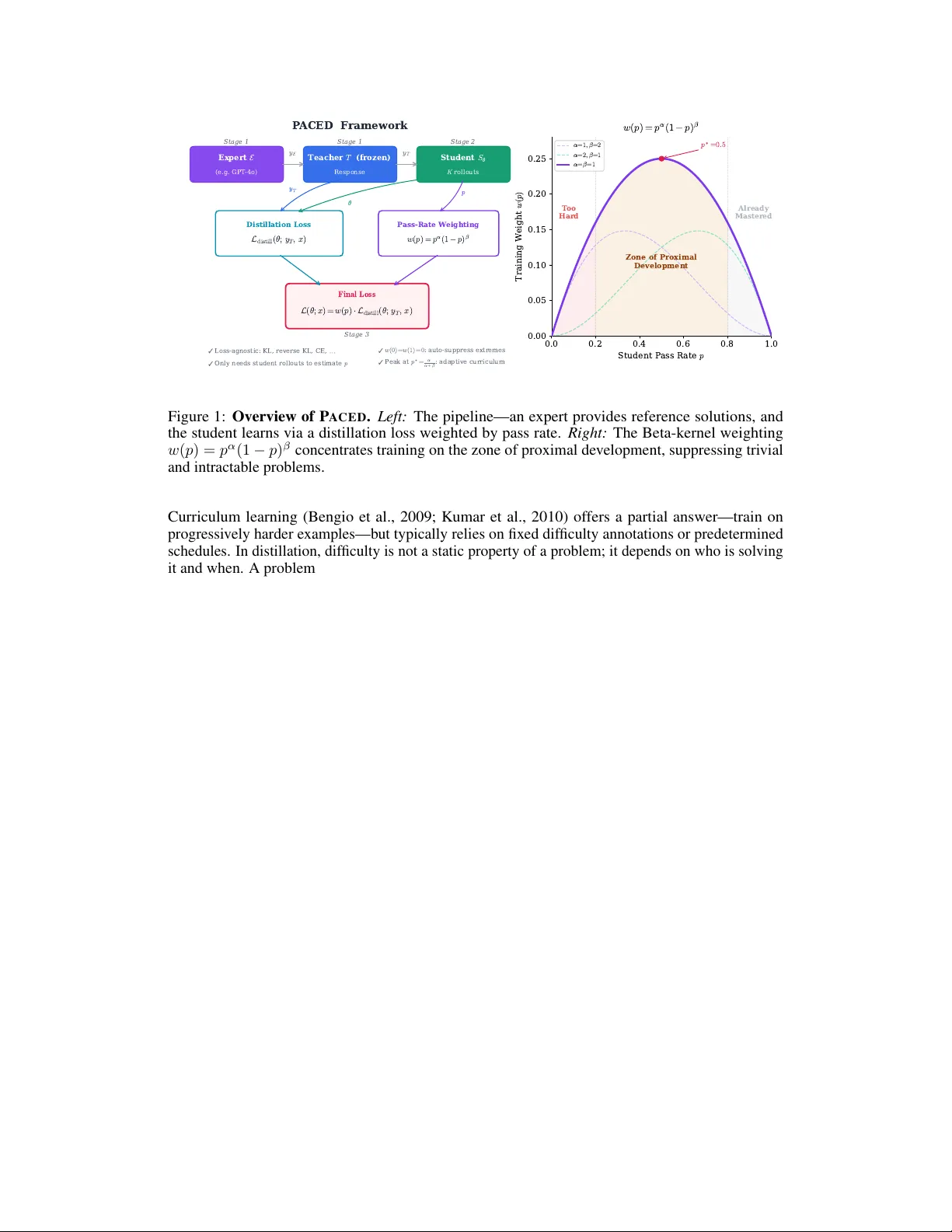
P AC E D : Distillation and Self-Distillation at the Fr ontier of Student Competence Y uanda Xu ∗† yuanda@math.princeton.edu Hejian Sang ∗ hejian@alumni.iastate.edu Zhengze Zhou ∗ zz433@cornell.edu Ran He ∗ rh2528@columbia.edu Zhipeng W ang zhipeng.wang@alumni.rice.edu Abstract Standard LLM distillation wastes compute on two fronts: problems the student has already mastered (near-zero gradients) and problems f ar beyond its reach (incoherent gradients that erode existing capabilities). W e show that this waste is not merely intuiti ve but structurally inevitable: the gr adient signal-to-noise ratio in distillation pr ovably vanishes at both pass-r ate extr emes . This theoretical observation leads to P AC ED , a framework that concentrates distillation on the zone of pr oximal development —the frontier of a student model’ s competence—via a principled pass-rate weight w ( p ) = p α (1 − p ) β deriv ed from the boundary- vanishing structure of distillation gradients. Key results. (1) Theory: W e prov e that the Beta k ernel w ( p ) = p α (1 − p ) β is a leading-order weight family arising from the SNR structure of distillation, and that it is minimax-r obust —under bounded multiplicati ve misspeciﬁcation, worst-case ef- ﬁciency loss is only O ( δ 2 ) both pointwise and in aggreg ate (Theorem 6). (2) Distil- lation: On Qwen3-14B → Qwen3-8B with forward KL, P AC E D achiev es + 7 . 5 on MA TH-500 and + 14 . 8 on AIME 2025 o ver the base model, while k eeping MMLU forgetting at just 0 . 2 % . (3) Self-distillation: On Qwen2.5-Math-7B-Instruct with rev erse KL, gains are + 9 . 8 and + 13 . 6 , respectively . (4) T wo-stage syn- ergy: A forward-KL-then-rev erse-KL schedule yields the strongest results in our setting, reaching +9 . 1 / + 15 . 2 / + 16 . 7 on MA TH-500/AIME 2024/AIME 2025— supporting a mode-coverage-then-consolidation interpretation of the distillation process. All conﬁgurations require only student rollouts to estimate pass rates, need no architectural changes, and are compatible with any KL direction. 1 Introduction Knowledge distillation trains a student model to imitate a teacher , yet the training budget is spread uniformly across all problems—a striking inef ﬁcienc y that, as we sho w formally , is deeply rooted in the gradient structure of distillation itself. On mastered problems ( p ≈ 1 ), gradients vanish— computation with no learning. On intractable problems ( p ≈ 0 ), gradients are large b ut directionally incoherent, activ ely eroding existing capabilities (French, 1999; Kirkpatrick et al., 2017). W e prove that this is not merely anecdotal: the gradient signal-to-noise ratio (SNR) in distillation pr ovably vanishes at both pass-rate boundaries (Proposition 2), and under po wer-la w regularity , the Beta kernel w ( p ) = p α (1 − p ) β arises as a leading-order weight family tracking this SNR proﬁle (Proposition 3). This places the zone of proximal development (Vygotski ˘ i and Cole, 1978)—the frontier between mastery and incompetence—on rigorous footing as a well-motiv ated training target. ∗ Equal contribution. † Correspondence to yuanda@math.princeton.edu Preprint. Under re view . P ACED F ramework y E y T Stage 1 Stage 1 Stage 2 y T θ p Stage 3 L o s s - a g n o s t i c : K L , r e v e r s e K L , C E , O n l y n e e d s s t u d e n t r o l l o u t s t o e s t i m a t e p w ( 0 ) = w ( 1 ) = 0 : a u t o - s u p p r e s s e x t r e m e s P e a k a t p ∗ = α α + β : a d a p t i v e c u r r i c u l u m E x p e r t E (e.g. GPT -4o) T e a c h e r T ( f r o z e n ) Response S t u d e n t S θ K r o l l o u t s Distillation Loss L d i s t i l l ( θ ; y T , x ) P ass-R ate W eighting w ( p ) = p α ( 1 − p ) β F i n a l L o s s L ( θ ; x ) = w ( p ) · L d i s t i l l ( θ ; y T , x ) 0.0 0.2 0.4 0.6 0.8 1.0 S t u d e n t P a s s R a t e p 0.00 0.05 0.10 0.15 0.20 0.25 T r a i n i n g W e i g h t w ( p ) p ∗ = 0 . 5 T oo Hard Zone of Proximal Development Already Mastered w ( p ) = p α ( 1 − p ) β α = 1 , β = 2 α = 2 , β = 1 α = β = 1 Figure 1: Overview of P AC E D . Left: The pipeline—an expert provides reference solutions, and the student learns via a distillation loss weighted by pass rate. Right: The Beta-kernel weighting w ( p ) = p α (1 − p ) β concentrates training on the zone of proximal de velopment, suppressing tri vial and intractable problems. Curriculum learning (Bengio et al., 2009; Kumar et al., 2010) of fers a partial answer —train on progressiv ely harder examples—b ut typically relies on ﬁxed dif ﬁculty annotations or predetermined schedules. In distillation, difﬁculty is not a static property of a problem; it depends on who is solving it and when. A problem that stumps the student in epoch 1 may become tractable by epoch 5. W e propose P roﬁciency- A dapti ve C ompetence E nhanced D istillation ( P AC E D ), a framew ork that automatically steers distillation tow ard the pr oblems wher e learning actually happens . The framework is loss-agnostic, architecture-agnostic, and requires only student rollouts. W e validate it across tw o cleanly separated settings: Distillation (Qwen3-14B → Qwen3-8B, forward KL) and Self-distillation (Qwen2.5-Math-7B-Instruct, rev erse KL), achie ving large gains on reasoning benchmarks (Y u et al., 2025) with near-zero for getting on MMLU (Hendrycks et al., 2021a). Our contributions are: 1. A theoretically derived curriculum (not a heuristic): the Beta-kernel weight w ( p ) = p α (1 − p ) β emerges as a leading-order family from the boundary-vanishing structure of distillation gradients, rather than from ad-hoc design. The default w ( p ) = p (1 − p ) requires zero h yperparameter tuning . 2. Minimax r obustness guarantee : e ven when the true gradient SNR deviates from the Beta model by a multiplicati v e factor e ± δ , worst-case ef ﬁciency loss is only O ( δ 2 ) —both pointwise and in aggregate (Theorem 6). For δ ≤ 0 . 3 (SNR 2 within 35% ), efﬁcienc y exceeds 91% . 3. Simultaneous plasticity and stability : P AC E D deliv ers +7 . 5 (MA TH-500) and +14 . 8 (AIME 2025) in the distillation track, and +9 . 8 / + 13 . 6 in self-distillation—while keeping MMLU forgetting at 0 . 2% and 0 . 6% , respecti vely . A two-stage schedule (forward KL → rev erse KL) pushes gains to +9 . 1 / + 15 . 2 / + 16 . 7 . 4. A unifying view of KL directions in distillation : the dual-track design re v eals that forw ard KL (mode cov erage) and re v erse KL (mode consolidation) are complementary stages of a single distillation process, not competing alternativ es. An ov ervie w appears in Figure 1. 2 Related W ork Knowledge Distillation. The idea of training a smaller model to mimic a larger one dates to Hinton et al. (2015), who showed that the “soft” distrib ution over classes carries richer information than hard labels alone. Since then, the ﬁeld has explored sequence-lev el distillation (Kim and Rush, 2016), 2 rev erse KL objectives (Gu et al., 2023; Agarwal et al., 2023), distribution-aligned methods (Y an et al., 2026; Y ang et al., 2024b), and regression-based approaches (Ba and Caruana, 2014; Kim et al., 2021; W ang et al., 2020). A common thread runs through this work: all samples are treated alike. Our contribution is to break this symmetry , letting the student’ s own competence determine where training effort ﬂo ws—regardless of the underlying loss function. Curriculum Lear ning. Bengio et al. (2009) articulated the principle that models beneﬁt from seeing easier examples ﬁrst. Self-paced learning (Kumar et al., 2010) and automated curriculum design (Grav es et al., 2017) extended this intuition in various directions. Howe ver , existing approaches typically rely on ﬁxed dif ﬁculty annotations or predetermined schedules. W e propose a ﬁner-grained, fully automatic alternati ve: a continuous Beta-kernel weight (Section 3.3) derived from gradient- efﬁcienc y maximization, which adapts smoothly as the student’ s competence e volv es—no manual thresholds or scheduling required. Sample Reweighting. Importance sampling can accelerate SGD by weighting each sample propor- tionally to its gradient norm (Katharopoulos and Fleuret, 2018), while meta-learning approaches learn per-sample weights end-to-end (Ren et al., 2018). Both demonstrate that non-uniform weighting improv es training, but dif fer from our setting in several ways: the former requires per-sample gradient norms (expensi ve for LLMs) and the latter requires a clean held-out set plus bi-le vel optimization; more fundamentally , both target supervised learning and do not address catastrophic forgetting. Our Beta-kernel weight is a closed-form function of the pass rate alone, theoretically grounded in the SNR structure of distillation gradients, and simultaneously serves both learning ef ﬁcienc y and forgetting prev ention by suppressing the boundary samples most responsible for capability degradation. In the RL setting, A CE (Xu et al., 2026) introduces per-rollout conﬁdence-based penalty modulation within GRPO/D APO, targeting o v erconﬁdent errors rather than uniformly penalizing all incorrect rollouts. While A CE operates at the r ollout level within RL training, P AC E D operates at the problem level within distillation; the two are complementary . On-Policy Distillation and Self-Distillation. GKD (Agarwal et al., 2023) trains the student on its own samples rather than the teacher’ s, narrowing the train-inference gap. SDFT (Shenfeld et al., 2026) takes this further: the same model plays both teacher (with demonstration context) and student (without), keeping the teacher’ s distribution close to the base policy and naturally reducing forgetting. Complementary recent work studies on-polic y self-distillation with pri vileged reasoning traces, where the same model teaches itself under dif ferent contexts on the student’ s own rollouts (Zhao et al., 2026). OPSDC (Sang et al., 2026) applies on-policy rev erse KL self-distillation to compress verbose chain-of-thought reasoning, conditioning the same model on a conciseness instruction to obtain teacher logits. Our framework shares the self-distillation backbone to some extent but is more general in two respects: it is not restricted to self-distillation—we also ev aluate with a larger same-f amily teacher (Qwen3-14B → Qwen3-8B)—and the pass-rate weighting is loss-agnostic, applicable to both forward and re verse KL (and potentially other objectiv es). Rather than compressing reasoning length, pass-rate weighting determines which problems to prioritize. Distillation already mitigates forgetting relativ e to SFT on hard labels, since soft tar gets preserve richer distrib utional information (Hinton et al., 2015; Shenfeld et al., 2026); we therefore adopt distillation as the training paradigm and focus on further improving it through principled sample weighting. Accordingly , SFT is not included as a baseline: the distillation-vs-SFT comparison is well established in prior work (Hinton et al., 2015; Kim and Rush, 2016; Gu et al., 2023; Shenfeld et al., 2026), and our contribution is orthogonal— improving how distillation allocates its training b udget, not whether distillation should be preferred ov er SFT . Catastrophic F orgetting. EWC (Kirkpatrick et al., 2017), GEM (Lopez-P az and Ranzato, 2017), and OGD (Farajtabar et al., 2019) all combat forgetting by constraining parameter updates. Our approach takes a different path: rather than adding explicit regularization, we prevent forgetting through curriculum design, ﬁltering out the training signals most likely to cause harm before they ev er reach the optimizer . 3 2.1 Method Positioning Summary T able 1: Method-feature comparison. ✓ = primary design characteristic. Featur e Self-Dist. AdaRFT AdaKD AKL P AC E D Adaptiv e weighting / curriculum ✓ ✓ ✓ ✓ Student-side competence signal ✓ ✓ Implicit forgetting reduction ✓ ✓ Loss-agnostic ✓ ✓ Theoretically grounded ✓ ✓ 3 Methodology P AC E D rests on a single core idea: a weighting scheme that directs distillation tow ard the problems where it can do the most good (Section 3.3). 3.1 Problem Setup W e use two disjoint training splits: D dist for distillation and D self for self-distillation. Let T denote the frozen teacher model and S θ the student model. In distillation, T is a larger same-f amily model (Qwen3-14B) and S θ is Qwen3-8B. In self-distillation, T is a frozen copy of Qwen2.5-Math-7B- Instruct and S θ is the trainable copy . In both settings, T is ﬁxed while θ is updated. For each prompt x , we sample K rollouts from the student and compute the pass rate : p ( x ; θ ) = 1 K K X k =1 1 h correct ( y ( k ) S , x ) i , y ( k ) S ∼ π θ ( · | x ) (1) The pass rate p ∈ [0 , 1] measures the student’ s current competence on problem x . 3.2 Reference Response Generation The most capable frontier models—gpt-oss-120b (OpenAI et al., 2025), Claude, Gemini—are accessible only through black-box APIs. W e obtain expert solutions via the API and use them as reference responses for distillation. Speciﬁcally , a frozen teacher model T generates a complete solution conditioned on the problem and the expert solution: y T ∼ P T ( y | x, y E ) (2) Because the teacher re-expresses the e xpert’ s reasoning in its own distrib utional v oice, the reference response is naturally within the model family’ s e xpressiv e range—a target the student can realistically aspire to. This design also turns black-box expert supervision into white-box distillation signals: once transferred into same-family teacher outputs, we can train on full token-le vel logits (forw ard/re verse KL), rather than being limited to hard-label SFT on API text alone. Figure 2 sho ws a concrete prompt template used in our pipeline: the student sees only the original problem, while the teacher additionally receiv es the expert solution as context. T eacher conﬁguration. T o keep the story clean, we bind one KL direction to each setting: distillation (Qwen3-14B → Qwen3-8B) uses forward KL, and self-distillation (Qwen2.5-Math-7B-Instruct) uses rev erse KL. This pairing reﬂects their roles: forward KL fa vors broad teacher -mode coverage when student–teacher capacity dif fers, while re verse KL fav ors compact, high-conﬁdence modes when teacher and student are near-polic y . 3.3 Pass-Rate W eighting Motivation. Not all training problems contribute equally . At one extreme ( p ≈ 0 ), the student cannot solve the problem at all; logit gradients are large b ut point in near-random directions across prompts, offering high variance and little useful signal. At the other extreme ( p ≈ 1 ), the student already matches the teacher; gradients are negligibly small. In practice a substantial fraction of problems f alls 4 Student Prompt π θ ( · | x ) Solve the following math problem step by step. The last line of your response should be of the form Answer: $Answer (without quotes) where $Answer is the answer to the problem. Find all real numbers x such that x 3 − 6 x 2 + 11 x − 6 = 0 . Remember to put your answer on its own line after “Answer:”. T eacher Prompt π ¯ θ ( · | x, y E ) Find all real numbers x such that x 3 − 6 x 2 + 11 x − 6 = 0 . Expert solution: {expert solution}. Treat it as guidance: understand the reasoning and then write the solution in your own words. Do not copy the original answer verbatim. Solve the following math problem step by step. The last line of your response should be of the form Answer: $Answer (without quotes) where $Answer is the answer to the problem. Find all real numbers x such that x 3 − 6 x 2 + 11 x − 6 = 0 . Remember to put your answer on its own line after “Answer:”. Figure 2: Prompt example for student and teacher policies. Both policies share the same model family b ut dif fer in conditioning context. The teacher receiv es the e xpert solution y E as additional context, while the student receiv es only the original problem. This contextual asymmetry enables black-box expert guidance to be transferred into white-box teacher logits for distillation. into these uninformativ e extremes—e.g., with Qwen3-8B on D APO, roughly 49% of problems hav e p < 0 . 2 or p > 0 . 8 (the exact proportion depends on the model and dataset). The richest—highest signal-to-noise ratio—gradient signal concentrates at intermediate difﬁculty , where the student is partially competent and each update carries genuine information. This raises a natural question: what is the principled weight function that exploits this structur e? Theoretical answer . In distillation, the gradient signal-to-noise ratio (SNR) vanishes at both bound- aries: at p → 0 (gradient incoherence) and p → 1 (alignment at mastery; Proposition 2). Under power -law regularity at the boundaries (Assumption 3(b)), any such SNR proﬁle decomposes as p a ′ (1 − p ) b ′ · e r ( p ) with bounded remainder (Proposition 3). The leading-order , maximum-parsimony weight family is therefore the Beta kernel: w ( p ) = p α (1 − p ) β (3) with peak at p ∗ = α/ ( α + β ) . The default choice α = β = 1 giv es w ( p ) = p (1 − p ) , which is symmetric around p ∗ = 0 . 5 , zero at the boundaries, and equals the in verse Bernoulli Fisher information (Remark 5). Asymmetric choices ( α  = β ) shift the peak to prioritize harder or easier problems. This form is minimax-robust: e ven when the true SNR proﬁle deviates from the Beta model by a multiplicati ve f actor e ± δ , the worst-case ef ﬁcienc y loss is only O ( δ 2 ) (Theorem 6). See Appendix A.4 for the full deriv ation. Crucially , having a realistic target is what makes pass-rate weighting meaningful: because y T is attainable (Section 3.2), the student’ s pass rate p genuinely reﬂects a learnable gap rather than an architectural mismatch, and the Beta kernel can reliably direct effort to where that gap is most productiv e. 5 Algorithm 1 P AC E D : Competence-A ware Distillation with Pass-Rate W eighting Require: Prompt dataset D , expert E , frozen teacher T , student S θ , distillation loss L distill (forward KL or rev erse KL), weight exponents ( α, β ) (def ault α = β =1 ), rollouts K 1: // Stage 1: T eacher -side target pr eparation (f orward KL only) 2: if L distill is forward KL then 3: for each prompt x ∈ D do 4: y E ← E ( x ) {Expert rollout (e.g., gpt-oss-120b solution)} 5: y T ← T ( · | x, y E ) {T eacher regeneration conditioned on expert solution} 6: end for 7: end if 8: // Stage 2: One-shot pass-rate estimation (paper setting) 9: for each prompt x i ∈ D do 10: Sample { y ( k ) S,i } K k =1 ∼ π θ ( · | x i ) 11: p i ← 1 K P k 1 [ correct ( y ( k ) S,i , x i )] 12: w i ← p α i (1 − p i ) β {Default: w i = p i (1 − p i ) } 13: end for 14: ˜ w i ← w i / ¯ w for all i {Normalize to unit mean and keep ﬁxed during training} 15: // Stage 3: W eighted Distillation 16: for each training iteration do 17: for each prompt x i ∈ D do 18: if L distill is forward KL then 19: L ( x i ) ← ˜ w i · L distill ( θ ; y T ,i , x i ) {T eacher-forced distillation} 20: else 21: Sample y S,i ∼ π θ ( · | x i ) 22: L ( x i ) ← ˜ w i · L distill ( θ ; y S,i , x i ) {Rev erse-KL self-distillation on student rollouts} 23: end if 24: end for 25: Update θ via gradient descent on 1 N P i L ( x i ) 26: end for 27: // Optional extension (not used in this paper): periodically recompute { p i , ˜ w i } 3.4 Overall Algorithm Putting the pieces together: each problem’ s contribution to the loss is scaled by how informati ve it is for the student right now: L ( θ ; x ) = w ( p ) · L distill ( θ ; x ) (4) where p = p ( x ; θ ) , w ( p ) = p (1 − p ) by default, and L distill is chosen by training setting. W e naturally use the two KL directions as follo ws: • Distillation track (Qwen3): Forward KL along the teacher sequence y T : P t D K L  p T ( · | y T , V ar ( ˜ w ) E [ s 2 ] (Prop 7) • Exponent selection: ( α ∗ +1) / ( α ∗ + β ∗ +2) = ¯ p Z , α ∗ + β ∗ = ¯ p Z (1 − ¯ p Z ) / V ar Z ( p ) − 3 (Prop 11) Result 1: Structural characterization of the Beta ker nel family (Pr opositions 2–3). In distillation, the gradient signal-to-noise ratio (SNR) vanishes at both pass-rate extremes: as p → 0 , gradients from different intractable problems become directionally incoherent, so SNR ( p ) → 0 ; as p → 1 , the student matches the teacher and the gradient signal vanishes. Under power -law boundary regularity (Assumption 3(b)), Proposition 3 sho ws that any such SNR proﬁle decomposes as SNR 2 ( p ) = p a ′ (1 − p ) b ′ · e r ( p ) with bounded remainder r . Setting the shape variation of r to zero (maximum parsimony) yields the Beta kernel p a ′ (1 − p ) b ′ as the natural weight family . In other words, the functional form is dictated by boundary structure, not introduced by optimization. Result 2: Minimax rob ustness guarantee (Theor em 6, Main Theor em). The Beta kernel is not only a con venient approximation: it is minimax-optimal at leading or der in the low-SNR r e gime over the non-parametric uncertainty set { ϕ : | log ϕ ( p ) | ≤ δ } induced by bounded remainder r . Concretely , if true SNR 2 deviates from the Beta model by at most a factor e ± δ , worst-case descent ef ﬁciency is sech 2 ( δ ) ≥ 1 − δ 2 , both pointwise (ﬁxed p ) and in aggregate (Theorem 6(iii)). For moderate misspeciﬁcation ( δ ≤ 0 . 3 , i.e., SNR 2 within 35% of the Beta model), aggre gate ef ﬁciency exceeds 91% . See Appendix A.4. Result 3: Batch-lev el gradient variance r eduction (Proposition 7). The intuition: Non-uniform weighting has two opposing ef fects on gradient variance: 1. Bad: Do wnweighting some samples reduces the effecti ve batch size, which increases variance. 2. Good: If we downweight samples that ha ve high gradient v ariance (noisy gradients), this decr eases v ariance. The r esolution: Which force wins? Let σ 2 eff and σ 2 unif denote the gradient variance under Beta-k ernel and uniform weighting, respectiv ely . Their ratio admits a revealing decomposition: R = 1 + V ar P ( ˜ w ) | {z } penalty from non-uniform weights + Cov P ( ˜ w 2 , s 2 ) E P [ s 2 ] | {z } coupling between weight and second moment − ∥ E P [ ˜ w g ] ∥ 2 E P [ s 2 ] | {z } mean-subtraction correction 1 − ∥ E P [ g ] ∥ 2 E P [ s 2 ] (6) where ˜ w is the normalized weight, g is the per-sample gradient, and s 2 ( p ) = E [ ∥ g ( p ) ∥ 2 ] is the gradient second moment at pass rate p . In the low-SNR re gime—where the mean terms are small relati ve to E P [ s 2 ] —the story simpliﬁes: v ariance reduction happens when the weight–second-moment cov ariance is sufﬁciently negati ve. 7 Why Beta kernels win this tug of war: When gradient variance runs hottest at e xtreme pass rates (As- sumption 3(c)), the Beta kernel assigns near -zero weight exactly where s 2 is largest, and concentrates weight where gradients carry real information. This targeted suppression of the noisiest samples can ov ercome the penalty of non-uniformity , yielding R < 1 and faster con vergence. Concrete parameter regimes are identiﬁed in Appendix A.5. Result 4: Data-driv en exponent selection (Proposition 11). The concern: The default α = β = 1 is a reasonable starting point, b ut can we do better? And can the theory tell us the optimal ( α, β ) from observable quantities, rather than requiring a grid search? The answer: Y es. The peak location p ∗ and kernel concentration can be determined by matching the kernel shape to the pass-rate distrib ution within the zone of proximal de velopment (ZPD). Concretely , deﬁne the ZPD as the set of problems with intermediate pass rates: Z = { i : ϵ ≤ p i ≤ 1 − ϵ } for a cutoff ϵ (e.g., ϵ = 1 /K ). Then the exponents can be estimated from two empirical moments of the pass-rate distrib ution restricted to Z . Since the kernel w ( p ) = p α (1 − p ) β normalized ov er [0 , 1] yields a Beta( α +1 , β +1) density , we apply standard moment matching to this distribution: α ∗ + 1 α ∗ + β ∗ + 2 = ¯ p Z , α ∗ + β ∗ = ¯ p Z (1 − ¯ p Z ) V ar Z ( p ) − 3 (7) where ¯ p Z and V ar Z ( p ) are the mean and v ariance of { p i } i ∈Z . The kernel peak p ∗ = α ∗ / ( α ∗ + β ∗ ) is approximately ¯ p Z for concentrated distributions. If the informati ve problems ha ve pass rates concentrated around 0 . 4 with low variance, the formula prescribes an asymmetric k ernel ( α ∗ < β ∗ ) peaked near p ∗ ≈ 0 . 4 ; if they are spread broadly , it prescribes a ﬂatter kernel (small α ∗ + β ∗ ). The formula requires no gradient computation—only the pass rates already computed for weighting. See Appendix A.6 for the deriv ation. For getting r eduction. Empirically , Beta-kernel weighting substantially reduces catastrophic forget- ting by suppressing gradient updates from boundary-pass-rate samples, which tend to carry noisy signals that erode prior capabilities; see T ables 4 and 5 for quantitativ e results. 4 Experiments 4.1 Experimental Setup • External Expert: gpt-oss-120b (OpenAI et al., 2025) for initial solution generation. • T eacher/Student Models (split by setting): – Distillation setting: Qwen3-8B (Y ang et al., 2025) as student, frozen Qwen3-14B as teacher , and forward KL as base loss. – Self-distillation setting: Qwen2.5-Math-7B-Instruct (Y ang et al., 2024a) with a frozen self-teacher , and reverse KL as base loss. In both settings, the teacher is frozen throughout training. • T raining data split: W e split D APO (Y u et al., 2025) into two disjoint partitions, one per setting. This av oids cross-setting leakage and k eeps the tw o narrati ves (distillation vs self-distillation) independently interpretable. • Evaluation: – Plasticity (new skill acquisition): mean@8 accuracy on MA TH-500 (Hendrycks et al., 2021b), AIME 2024, and AIME 2025 (out-of-distribution generalization). For each problem, we sample 8 responses (temperature 0.6, top- p 0.95) and report mean@8. – Stability (retention of prior knowledge): MMLU (Hendrycks et al., 2021a). • Rollouts: K = 8 rollouts per problem for pass-rate estimation. • Pass-rate weight: Default w ( p ) = p (1 − p ) (i.e., α = β = 1 ). In this paper , pass rates are estimated once before optimization; the resulting weights are normalized to unit mean (i.e., ˜ w i = w i / ¯ w ) and then kept ﬁx ed during training. • Baselines (setting-speciﬁc): – Distillation/Qwen3: Forward KL (unweighted), Hard Filter F orward KL, AKL, and P AC E D Forw ard KL. 8 – Self-distillation/Qwen2.5: Re verse KL (unweighted), Hard Filter Re verse KL, AKL, and P AC E D Re verse KL. – AKL (W u et al., 2025): An adapti ve KL di ver gence baseline that dynamically adjusts the per-tok en KL coefﬁcient based on the discrepancy between student and teacher logits. Unlike P AC E D , which operates at the pr oblem level (weighting entire problems by pass rate), AKL operates at the token level (modulating the KL penalty at each decoding step). AKL requires no rollout or pass-rate estimation—the adaptiv e coef- ﬁcient is computed from teacher–student logit differences during training. All other hyperparameters (learning rate, batch size, number of epochs) are kept identical to the corresponding unweighted baseline. 4.2 Main Results (Plasticity-Stability T rade-off) T able 2: Distillation track (Qwen3-14B → Qwen3-8B, forward KL family): reasoning performance (mean@8). ↑ = higher is better . Method MA TH-500 ( ↑ ) AIME 24 ( ↑ ) AIME 25 ( ↑ ) Base 86.5% 28.7% 20.8% Forward KL (unweighted) 90.4% 35.9% 29.3% Hard Filter Forward KL 92.7% 39.5% 33.9% AKL 91.9% 39.8% 34.1% P AC E D Forward KL 94.0% 41.6% 35.6% T able 3: Self-distillation track (Qwen2.5-Math-7B-Instruct, rev erse KL family): reasoning perfor- mance (mean@8). Method MA TH-500 ( ↑ ) AIME 24 ( ↑ ) AIME 25 ( ↑ ) Base 83.9% 19.6% 11.5% Rev erse KL (unweighted) 90.4% 25.3% 16.9% Hard Filter Rev erse KL 92.0% 28.9% 22.0% AKL 91.4% 28.2% 21.5% P AC E D Reverse KL 93.7% 31.6% 25.1% T able 4: Retention in distillation track (Qwen3 forward KL family): MMLU and forgetting ( ∆ from base). Method MMLU ( ↑ ) For getting ( ↓ ) W eighting Base 73.2% – – Forward KL (unweighted) 66.4% 6.8% None Hard Filter Forward KL 70.7% 2.5% Hard AKL 68.6% 4.6% T oken-lev el P AC E D Forward KL 73.0% 0.2% Beta Reasoning (T ables 2 and 3). W ith the split-track protocol, the pattern is consistent in both settings. In the distillation track (Qwen3, forw ard KL family), P AC E D improv es MA TH-500 from 90 . 4% to 94 . 0% and boosts AIME 2024/2025 by +5 . 7 / + 6 . 3 points over unweighted forward KL. In the self-distillation track (Qwen2.5, reverse KL family), P AC E D improv es MA TH-500 from 90 . 4% to 93 . 7% and boosts AIME 2024/2025 by +6 . 3 / + 8 . 2 points o v er unweighted rev erse KL. AKL baseline comparison. AKL (W u et al., 2025) is a strong baseline that also adapts the distillation signal dynamically , but at a fundamentally dif ferent granularity: it modulates the KL coefﬁcient per token based on teacher –student logit discrepancy , whereas P AC E D modulates per pr oblem based on pass rate. AKL improv es ov er unweighted training, conﬁrming that adaptiv e weighting is beneﬁcial. Howe ver , P AC E D consistently outperforms AKL on all reasoning benchmarks in both tracks (e.g., +2 . 1 / + 1 . 8 / + 1 . 5 on MA TH-500/AIME 24/AIME 25 in distillation; +2 . 3 / + 3 . 4 / + 3 . 6 in self- distillation), with comparable or lower for getting. The gap reﬂects a structural difference between 9 T able 5: Retention in self-distillation track (Qwen2.5 reverse KL f amily): MMLU and forgetting ( ∆ from base). Method MMLU ( ↑ ) For getting ( ↓ ) W eighting Base 70.6% – – Rev erse KL (unweighted) 68.4% 2.2% None Hard Filter Reverse KL 70.1% 0.5% Hard AKL 69.8% 0.8% T oken-lev el P AC E D Re verse KL 70.0% 0.6% Beta token-le vel and problem-le v el adaptation. AKL adjusts how much the student learns from each token within a given problem, but treats all problems equally—an intractable problem ( p ≈ 0 ) recei ves the same total training b udget as a producti ve one ( p ≈ 0 . 5 ). This means AKL cannot suppress the noisy , high-variance gradie nts from intractable problems or the redundant gradients from mastered ones; it only rebalances within each problem. In contrast, P AC E D operates at the problem le vel via a continuous Beta kernel w ( p ) = p α (1 − p ) β , concentrating the entire training b udget on problems where the student has partial competence. Notably , the two approaches are orthogonal and could in principle be combined: P AC E D selects which problems to train on, while AKL optimizes how to train on each selected problem. Stability (T ables 4 and 5). For getting reduction remains strong after splitting by setting. In distillation, P AC E D forward KL reduces forgetting from 6 . 8 to 0 . 2 points. In self-distillation, rev erse- KL-based methods already forget less, and P A C E D keeps for getting in the low range ( 0 . 6 points) while preserving the largest reasoning g ains. AKL reduces for getting relati ve to unweighted training—its per-tok en adaptation implicitly down-weights tok ens where the teacher–student gap is e xtreme—but P AC E D still achie ves lo wer or comparable forgetting in both tracks. The dif ference is that AKL cannot suppress entire intractable problems: even with per-token adaptation, passing gradients through a p ≈ 0 problem injects noise that accumulates across tokens. 4.3 Ablation Studies (V alidating Each Component’ s Necessity) 4.3.1 Effect of W eight Exponents Ablations in this section use Qwen3-8B as the primary model. T able 6: Ablation on pass-rate weight e xponents w ( p ) = p α (1 − p ) β using forward KL di vergence as the distillation loss (Qwen3-8B). α β MA TH-500 ( ↑ ) Forgetting on MMLU ( ↓ ) 1 1 94.0% 0.2% 1 2 95.4% 0.9% 2 1 91.5% 1.8% 1 3 94.9% 2.4% 3 1 90.3% 1.7% Interpr etation. The ablation re veals a clear trade-of f between reasoning gains and forgetting as the kernel shape shifts. The asymmetric kernel ( α =1 , β =2) peaks at p ∗ = 1 / 3 , tilting the curriculum tow ard harder problems; this yields the strongest MA TH-500 score ( 95 . 4% , +1 . 4 ov er default) but increases forgetting to 0 . 9% . Pushing further to ( α =1 , β =3) peaks at p ∗ = 1 / 4 and sho ws diminishing returns ( 94 . 9% ) with sharply higher forgetting ( 2 . 4% ), suggesting that weighting too- difﬁcult problems e ventually reintroduces the noisy-gradient problem the kernel is designed to av oid. In the opposite direction, kernels that peak at easier problems— ( α =2 , β =1) and ( α =3 , β =1) — degrade MA TH-500 to 91 . 5% and 90 . 3% , respecti vely , while also increasing forgetting ( 1 . 8% and 1 . 7% ). This asymmetry corroborates the theoretical prediction: the student’ s ZPD mean ¯ p Z lies below 0 . 5 on D APO, so the optimal peak should lean toward harder problems. The default ( α = β =1) offers the best ov erall balance—strong reasoning improv ement with near-zero for getting ( 0 . 2% )—making it a robust def ault when the plasticity–stability trade-of f matters. 10 4.3.2 Sensitivity to Number of Rollouts K The pass-rate estimate ˆ p i = ( # correct out of K ) controls the Beta kernel weights. W e ablate K ∈ { 4 , 8 , 16 } on Qwen3-8B distillation (forw ard KL, α = β =1 ) to test (i) how estimation noise from small K affects ﬁnal performance, (ii) whether large K yields further gains, and (iii) the associated compute cost. T able 7: Sensitivity to number of rollouts K for pass-rate estimation. All results use Qwen3-8B with forward KL and default e xponents ( α = β =1) . K MA TH-500 ( ↑ ) AIME 24 ( ↑ ) AIME 25 ( ↑ ) MMLU Fgt. ( ↓ ) 4 92.8% 40.1% 34.2% 0.2% 8 94.0% 41.6% 35.6% 0.2% 16 94.5% 42.5% 36.2% 0.3% Interpr etation. Halving the rollout budget to K =4 costs only 1 . 2 points on MA TH-500 and 1 . 4 on AIME 25, while forgetting remains unchanged at 0 . 2% . This conﬁrms that the Beta kernel’ s smooth weighting is rob ust to the noisier pass-rate estimates from small K —unlike hard-threshold ﬁlters, a continuous weight function does not amplify estimation errors near the decision boundary . Doubling to K =16 yields marginal gains ( +0 . 5 MA TH-500, +0 . 6 AIME 25) with diminishing returns, suggesting K =8 strikes a practical balance between estimation quality and rollout cost. These results also quantify the compute o verhead: the pass-rate estimation phase scales linearly in K , so K =4 halves the inference b udget relati ve to K =8 with only modest accuracy loss, of fering a useful knob when compute is constrained. 4.3.3 Why F orward KL for Distillation and Reverse KL f or Self-Distillation The Beta kernel controls whic h problems to train on; KL direction controls how probability mass is transferred. • Forward KL ( KL( p T ∥ p S ) ) is mode-cov ering. In the Qwen3 distillation setting, the larger teacher contains broader reasoning modes; forw ard KL encourages the smaller student to cov er them rather than collapsing early . • Rev erse KL ( KL( p S ∥ p T ) ) is mode-seeking. In the Qwen2.5 self-distillation setting, teacher and student are near-polic y; re verse KL sharpens the student to ward conﬁdent high-quality modes and stabilizes outputs. T o make this asymmetry explicit rather than only conceptual, we report a direct two-stage order comparison in T able 8. In this two-stage setting, pass rates are recomputed once between stages so that Stage 2 uses weights matched to the student’ s updated competence after Stage 1. T able 8: T wo-stage order comparison on Qwen3 with the same pass-rate weighting w ( p ) = p (1 − p ) . Pass rates are recomputed once between stages; the ﬁrst half of training steps uses Stage 1 and the second half uses Stage 2. Results are mean@8. The ﬁrst two rows are single-loss references and the last two ro ws isolate schedule order . Stage 1 Stage 2 MA TH-500 ( ↑ ) AIME 24 ( ↑ ) AIME 25 ( ↑ ) MMLU Fgt. ( ↓ ) Paced KL P aced KL 94.0% 41.6% 35.6% 0.2% Paced Re vKL Paced RevKL 93.2% 40.9% 35.3% 0.1% Paced Re vKL Paced KL 92.1% 38.9% 33.7% 0.3% Paced KL Paced Re vKL 95.6% 43.9% 37.5% 0.1% T akeaway . The order effect is large and consistent: KL → RevKL impro ves o ver single-loss Paced KL by +1 . 6 (MA TH-500), +2 . 3 (AIME 24), and +1 . 9 (AIME 25), while rev ersing the order (Re vKL → KL) underperforms both single-loss baselines. This directly supports the paper’ s narrati ve: mode-cov ering ﬁrst for exploration, then mode-seeking for consolidation. This giv es a natural bridge in the paper’ s logic: ﬁrst present cross-model distillation where cov erage is the priority (forward KL), then present self-distillation where consolidation is the priority (re verse 11 T able 9: Ablation on the fraction of training steps allocated to Stage 1 for two-stage distillation on Qwen3 under the KL → RevKL schedule. The ﬁrst x % of steps use Paced KL (Stage 1) and the remaining steps use Paced Re vKL (Stage 2). Results are mean@8. Schedule Stage 1 ratio MA TH-500 ( ↑ ) AIME 24 ( ↑ ) AIME 25 ( ↑ ) MMLU Fgt. ( ↓ ) KL → RevKL 25% 94.7% 42.1% 36.3% 0.1% KL → RevKL 50% 95.6% 43.9% 37.5% 0.1% KL → RevKL 75% 95.2% 43.1% 37.0% 0.2% KL). In both cases, pass-rate weighting is identical and remains the common mechanism for selecting informativ e samples. 4.4 Deep Analysis (V alidating Theory and Mechanisms: Gradients, Curriculum Evolution, etc.) Pass-Rate Distribution. At initialization, roughly 17% of problems have p < 0 . 2 and 32% hav e p > 0 . 8 , leaving about 51% in the productive middle range (T able 10). The p (1 − p ) kernel recognizes this imbalance and responds accordingly , assigning near-zero weight to the crowded tails and concentrating training on the informativ e minority . 4.4.1 Curriculum Progr ession T able 10 traces the migration of problems through the difﬁculty landscape during training using checkpointed pass-rate re-ev aluation. As the student strengthens, problems ﬂow steadily from the “too hard” regime ( p < 0 . 2 ) through the zone of proximal de velopment ( p ∈ [0 . 2 , 0 . 8] ) and into the “mastered” side ( p > 0 . 8 ): the fraction with p > 0 . 8 grows from 32% to 74% ov er 300 steps, while the av erage pass rate ¯ p rises monotonically from 0 . 61 to 0 . 84 . Notably , the Med- p bin shrinks from 51% to 21% , indicating that the pool of maximally informative problems is gradually depleted as the student masters more of the curriculum. This progressive depletion has a practical implication: the ef fectiv e training signal weakens ov er time as fewer problems remain in the ZPD, which is consistent with the diminishing marginal returns typical of later training stages and naturally favors more consolidativ e objectives (e.g., re verse-KL behavior) once the ZPD has substantially contracted. The low- p tail also shrinks (from 17% to 5% ), indicating that pre viously intractable problems gradually become tractable. This matters operationally in v ariants that recompute pass rates—such as our two- stage schedule, which re-estimates them once between stages—because ne wly accessible problems then receiv e larger weights after they enter the ZPD. T able 10: Evolution of the pass-rate distribution and av erage pass rate ¯ p across training. The distillation signal peaks when most problems enter the p ∈ [0 . 2 , 0 . 8] zone. T raining Stage Low p ( < 0 . 2 ) Med p ( 0 . 2 – 0 . 8 ) High p ( > 0 . 8 ) A vg pass rate ¯ p Step 0 (Init) 17% 51% 32% 0.61 Step 100 12% 32% 56% 0.70 Step 200 9% 24% 67% 0.78 Step 300 5% 21% 74% 0.84 4.4.2 Empirical Gradient SNR vs. Pass Rate Figure 3 provides direct empirical v alidation of the theoretical SNR prediction. For each problem i , we sample K =10 rollouts and compute the distillation loss gradient with respect to the lm_head parameters for each rollout, yielding gradient vectors g (1) i , . . . , g ( K ) i . W e then measure the per- problem SNR: d SNR i = ∥ ¯ g i ∥ 2 q 1 K P K k =1 ∥ g ( k ) i − ¯ g i ∥ 2 2 , ¯ g i = 1 K P k g ( k ) i , (8) where the numerator measures the magnitude of the mean gradient (signal) and the denominator measures the spread across rollouts (noise). Since both are norms, d SNR i ≥ 0 . W e then group 12 problems into equal-width pass-rate bins and compute the mean d SNR within each bin; the bin means are rescaled to [0 , 1] by dividing by the lar gest bin mean. The bell-shaped proﬁle predicted by Proposition 2 is clearly visible: SNR peaks at intermediate pass rates and is substantially lower at both boundaries, closely tracking the default p (1 − p ) kernel. 0.0 0.2 0.4 0.6 0.8 1.0 P a s s r a t e p ( b i n n e d ) 0.0 0.2 0.4 0.6 0.8 1.0 Normalized SNR (mean) Binned Gradient SNR vs. P ass R ate Figure 3: Empirical gradient SNR vs. student pass rate (Qwen3-8B, forward KL, K =10 rollouts). Gradients are computed at lm_head . Per-problem SNR values are av eraged within each pass-rate bin; bin means are then normalized to [0 , 1] by di viding by the maximum bin mean. Red bars mark boundary regions ( p < 0 . 2 or p > 0 . 8 ) where SNR is substantially lo wer; green bars mark the zone of proximal dev elopment where training signal is richest. 5 Discussion: Limitations and Future W ork Sev eral limitations deserve candid acknowledgment. Rollout overhead. Pass-rate estimation requires K rollouts per problem per recomputation epoch. As discussed in Section 3.4, the cost is amortized across training steps and shared with rev erse KL sampling; a two-phase screening strategy ( K init ≈ 4 ) can further reduce inference by early-exiting on problems with ˆ p ∈ { 0 , 1 } . The Beta kernel’ s smooth weighting is robust to noisy pass-rate estimates from moderate K (we use K =8 ), unlike hard ﬁlters that require precise thresholding. Exponent selection. The closed-form method (Proposition 11) is a moment-matching heuristic; fully adaptiv e online estimation via gradient SNR tracking remains an open problem. Future work. Sev eral directions remain open. (i) Continuous loss interpolation: the two-stage schedule switches from forward KL to rev erse KL at a ﬁxed midpoint; a natural extension is continuous interpolation L = (1 − λ t ) KL fwd + λ t KL rev with λ t driv en by ZPD statistics. (ii) Cr oss- ar c hitectur e and multi-teacher distillation: pass-rate weighting is deﬁned from student-side pass rates and may transfer naturally to cross-architecture settings (e.g., 70B → 7B), where capacity mismatch pushes more problems into the p ≈ 0 tail; multi-teacher ensembles—weighting each teacher –problem pair by student competence—are another natural extension. 6 Conclusion A good teacher does not drill ev ery problem with equal intensity—spending more time where a student struggles, moving p ast what is already mastered, and deferring what is still out of reach. P AC E D operationalizes this principle for LLM distillation: Beta-kernel pass-rate weighting (Eq. (3) ) concentrates gradient b udget on the frontier of a student’ s competence while suppressing unin- formativ e extremes. This weighting is not a design heuristic but a theoretical consequence—the 13 Beta kernel family arises as a leading-order characterization of the boundary-vanishing structure of distillation gradients (Propositions 2 – 3), and is minimax-robust under bounded misspeciﬁcation with worst-case efﬁciency loss O ( δ 2 ) (Theorem 6). Empirically , in a split-track protocol (Qwen3 distillation with forward KL, Qwen2.5 self-distillation with rev erse KL), P AC E D deli vers substantial reasoning gains ov er corresponding baselines while incurring lo w retention loss, demonstrating that plasticity and stability need not be at odds. Because the weighting depends only on student rollouts, it is directly compatible with alternati ve objecti ves and training topologies; broader cross-architecture and multi-teacher validation remains future w ork. References Rishabh Agarwal, Nino V ieillard, Y ongchao Zhou, Piotr Stanczyk, Sabela Ramos, Matthieu Geist, and Oli vier Bachem. On-policy distillation of language models: Learning from self-generated mistakes. arXiv pr eprint arXiv:2306.13649 , 2023. URL . Jimmy Ba and Rich Caruana. Do deep nets really need to be deep? NeurIPS , 2014. Y oshua Bengio, Jérôme Louradour, Ronan Collobert, and Jason W eston. Curriculum learning. ICML , 2009. Mehrdad F arajtabar , Navid Azizan, Alex Mott, and Ang Li. Orthogonal gradient descent for continual learning. arXiv preprint , 2019. URL . Robert M French. Catastrophic forgetting in connectionist networks. T r ends in Cognitive Sciences , 3 (4):128–135, 1999. Saeed Ghadimi and Guanghui Lan. Stochastic ﬁrst- and zeroth-order methods for nonconv ex stochastic programming. SIAM J ournal on Optimization , 23(4):2341–2368, 2013. Alex Gra ves, Marc G Bellemare, Jacob Menick, Rémi Munos, and K oray Kavukcuoglu. Automated curriculum learning for neural networks. ICML , 2017. Y uxian Gu, Li Dong, Furu W ei, and Minlie Huang. MiniLLM: On-policy distillation of large language models. CoRR , 2023. URL . Dan Hendrycks, Collin Burns, Ste v en Basart, Andy Zou, Mantas Mazeika, Da wn Song, and Jacob Steinhardt. Measuring massi ve multitask language understanding. Pr oceedings of ICLR , 2021a. Dan Hendrycks, Collin Burns, Saurav Kada v ath, Akul Arora, Ste ven Basart, Eric T ang, Dawn Song, and Jacob Steinhardt. Measuring mathematical problem solving with the MA TH dataset. NeurIPS , 2021b. Geoffre y Hinton, Oriol V inyals, and Jef f Dean. Distilling the kno wledge in a neural network. arXiv pr eprint arXiv:1503.02531 , 2015. Angelos Katharopoulos and François Fleuret. Not all samples are created equal: Deep learning with importance sampling. In International Confer ence on Machine Learning (ICML) , 2018. T aehyeon Kim, Jaehoon Oh, NakY oung Kim, Sangheum Cho, and Se-Y oung Y un. Comparing kullback-leibler di ver gence and mean squared error loss in kno wledge distillation. arXiv pr eprint arXiv:2105.08919 , 2021. Y oon Kim and Alexander M Rush. Sequence-level kno wledge distillation. In Pr oceedings of the Confer ence on Empirical Methods in Natural Languag e Processing , 2016. URL https: //arxiv.org/abs/1606.07947 . James Kirkpatrick, Razvan P ascanu, Neil Rabino witz, Joel V eness, Guillaume Desjardins, Andrei A. Rusu, Kieran Milan, John Quan, Tiago Ramalho, Agnieszka Grabska-Barwinska, Demis Hassabis, Claudia Clopath, Dharshan K umaran, and Raia Hadsell. Ov ercoming catastrophic for getting in neural networks. Pr oceedings of the National Academy of Sciences , 114(13):3521–3526, 2017. M Paw an Kumar , Benjamin Packer , and Daphne K oller . Self-paced learning for latent v ariable models. NeurIPS , 2010. David Lopez-Paz and Marc’Aurelio Ranzato. Gradient episodic memory for continual learning. NeurIPS , 2017. OpenAI, Sandhini Agarwal, Lama Ahmad, Jason Ai, Sam Altman, Andy Applebaum, Edwin Arbus, Rahul K. Arora, Y u Bai, Bo wen Baker , Haiming Bao, Boaz Barak, Ally Bennett, T yler Bertao, Niv edita Brett, Eugene Bre vdo, Greg Brockman, Sebastien Bubeck, Che Chang, Kai Chen, Mark 14 Chen, Enoch Cheung, Aidan Clark, Dan Cook, Marat Dukhan, Casey Dv orak, K e vin Fiv es, Vlad Fomenk o, T imur Garipov , Kristian Georgie v , Mia Glaese, T arun Gogineni, Adam Goucher , Lukas Gross, Katia Gil Guzman, John Hallman, Jackie Hehir , Johannes Heidecke, Alec Helyar , Haitang Hu, Romain Huet, Jacob Huh, Saachi Jain, Zach Johnson, Chris K och, Irina Kofman, Dominik Kundel, Jason Kwon, V olodymyr K yrylov , Elaine Y a Le, Guillaume Leclerc, James Park Lennon, Scott Lessans, Mario Lezcano-Casado, Y uanzhi Li, Zhuohan Li, Ji Lin, Jordan Liss, Lily Liu, Jiancheng Liu, Kevin Lu, Chris Lu, Zoran Martinovic, Lindsay McCallum, Josh McGrath, Scott McKinney , Aidan McLaughlin, Song Mei, Ste ve Mostov oy , T ong Mu, Gideon Myles, Alexander Neitz, Ale x Nichol, Jakub Pachocki, Alex Paino, Dana Palmie, Ashley Pantuliano, Giambattista Parascandolo, Jongsoo Park, Leher Pathak, Carolina Paz, Ludovic Peran, Dmitry Pimenov , Michelle Pokrass, Elizabeth Proehl, Huida Qiu, Gaby Raila, Filippo Raso, Hongyu Ren, Kimmy Richardson, David Robinson, Bob Rotsted, Hadi Salman, Suv ansh Sanjee v , Max Schwarzer , D. Sculley , Harshit Sikchi, K endal Simon, Karan Singhal, Y ang Song, Dane Stuckey , Zhiqing Sun, Philippe T illet, Sam T oizer , Foi v os Tsimpourlas, Nikhil Vyas, Eric W allace, Xin W ang, Miles W ang, Oli via W atkins, Ke vin W eil, Amy W endling, Ke vin Whinnery , Cedric Whitne y , Hannah W ong, Lin Y ang, Y u Y ang, Michihiro Y asunaga, Kristen Y ing, W ojciech Zaremba, W enting Zhan, Cyril Zhang, Brian Zhang, Eddie Zhang, a nd Shengjia Zhao. gpt-oss-120b & gpt-oss-20b Model Card, 2025. URL . Mengye Ren, W enyuan Zeng, Bin Y ang, and Raquel Urtasun. Learning to re weight examples for robust deep learning. In International Conference on Mac hine Learning (ICML) , 2018. Hejian Sang, Y uanda Xu, Zhengze Zhou, Ran He, Zhipeng W ang, and Jiachen Sun. On-policy self-distillation for reasoning compression. arXiv pr eprint arXiv:2603.05433 , 2026. Idan Shenfeld, Mehul Damani, Jonas Hübotter , and Pulkit Agraw al. Self-distillation enables continual learning. arXiv preprint , 2026. URL . Naftali T ishby , Fernando C Pereira, and William Bialek. The information bottleneck method. arXiv pr eprint physics/0004057 , 2000. L. S. Vygotski ˘ i and Michael Cole. Mind in Society: The Development of Higher Psychological Pr ocesses . Harvard Uni versity Press, 1978. W enhui W ang, Furu W ei, Li Dong, Hangbo Bao, Nan Y ang, and Ming Zhou. Minilm: Deep self- attention distillation for task-agnostic compression of pre-trained transformers. CoRR , 2020. URL https://arxiv.org/abs/2002.10957 . T aiqiang W u, Chaofan T ao, Jiahao W ang, Runming Y ang, Zhe Zhao, and Ng ai W ong. Rethinking Kullback-Leibler di v ergence in kno wledge distillation for large language models. In Pr oceedings of the 31st International Confer ence on Computational Linguistics (COLING) , pages 5737–5755, 2025. Y uanda Xu, Hejian Sang, Zhengze Zhou, Ran He, and Zhipeng W ang. Overconﬁdent errors need stronger correction: Asymmetric conﬁdence penalties for reinforcement learning. arXiv pr eprint arXiv:2602.21420 , 2026. Shaotian Y an, Kaiyuan Liu, Chen Shen, Bing W ang, Sinan Fan, Jun Zhang, Y ue W u, Zheng W ang, and Jieping Y e. Distribution-aligned sequence distillation for superior long-cot reasoning. arXiv pr eprint arXiv:2601.09088 , 2026. An Y ang, Beichen Zhang, Binyuan Hui, Bofei Gao, Bowen Y u, Chengpeng Li, Dayiheng Liu, Jianhong T u, Jingren Zhou, Junyang Lin, Keming Lu, Mingfeng Xue, Runji Lin, T ianyu Liu, Xingzhang Ren, and Zhenru Zhang. Qwen2.5-math technical report: T ow ard mathematical expert model via self-improv ement. arXiv pr eprint arXiv:2409.12122 , 2024a. An Y ang, Anfeng Li, Baosong Y ang, Beichen Zhang, Binyuan Hui, Bo Zheng, Bo wen Y u, Chang Gao, Chengen Huang, Chenxu Lv , Chujie Zheng, Dayiheng Liu, Fan Zhou, Fei Huang, Feng Hu, Hao Ge, Haoran W ei, Huan Lin, Jialong T ang, Jian Y ang, Jianhong T u, Jianwei Zhang, Jianxin Y ang, Jiaxi Y ang, Jing Zhou, Jingren Zhou, Junyang Lin, Kai Dang, Keqin Bao, K exin Y ang, Le Y u, Lianghao Deng, Mei Li, Mingfeng Xue, Mingze Li, Pei Zhang, Peng W ang, Qin Zhu, Rui Men, Ruize Gao, Shixuan Liu, Shuang Luo, T ianhao Li, T ianyi T ang, W enbiao Y in, Xingzhang Ren, Xinyu W ang, Xinyu Zhang, Xuancheng Ren, Y ang Fan, Y ang Su, Y ichang Zhang, Y inger Zhang, Y u W an, Y uqiong Liu, Zekun W ang, Zeyu Cui, Zhenru Zhang, Zhipeng Zhou, and Zihan Qiu. Qwen3 technical report. arXiv pr eprint arXiv:2505.09388 , 2025. 15 Zongyuan Y ang, Baolin Liu, Y ingde Song, Y ongping Xiong, Lan Y i, Zhaohe Zhang, and Xunbo Y u. Directl: Efﬁcient radiance ﬁelds rendering for 3d light ﬁeld displays. arXiv preprint arXiv:2407.14053 , 2024b. Qiying Y u, Zheng Zhang, Ruofei Zhu, Y ufeng Y uan, Xiaochen Zuo, Y u Y ue, W einan Dai, T iantian Fan, Gaohong Liu, Lingjun Liu, Xin Liu, Haibin Lin, Zhiqi Lin, Bole Ma, Guangming Sheng, Y uxuan T ong, Chi Zhang, Mofan Zhang, W ang Zhang, Hang Zhu, Jinhua Zhu, Jiaze Chen, Jiangjie Chen, Chengyi W ang, Hongli Y u, Y uxuan Song, Xiangpeng W ei, Hao Zhou, Jingjing Liu, W ei- Y ing Ma, Y a-Qin Zhang, Lin Y an, Mu Qiao, Y onghui W u, and Mingxuan W ang. D APO: An open-source llm reinforcement learning system. arXiv pr eprint arXiv:2503.14476 , 2025. Siyan Zhao, Zhihui Xie, Mengchen Liu, Jing Huang, Guan Pang, Feiyu Chen, and Aditya Grov er . Self-distilled reasoner: On-policy self-distillation for large language models. arXiv preprint arXiv:2601.18734 , 2026. URL . 16 A Complete Proofs Proof r oadmap. T o keep the narrati ve intuitiv e while preserving logical rigor , we use the follo wing dependency order: 1. Establish boundary conditions for distillation gradients (Proposition 2) and the boundary-to- Beta representation theorem (Proposition 3). 2. Use these structural results to obtain the non-monotonic learning-signal statement as a corollary-style consequence (Proposition 1). 3. Deri ve the descent-optimal weighting form and its robust minimax interpretation (Theorem 4, Theorem 6), then analyze variance and con ver gence. A.0 Notation and Assumptions Notation. Throughout the appendix, p ∈ [0 , 1] denotes the student pass rate for a problem, and w ( p ) ≥ 0 denotes its pass-rate weight (typically a Beta kernel w ( p ) = p α (1 − p ) β ). W e collect the shared assumptions here to av oid forward references in later proofs. Symbol guide. Three distinct pairs of exponents appear in the analysis and should not be confused: • ( a s , b s ) : signal e xponents —gov ern ho w the expected gradient norm ∥ E [ g ( p )] ∥ scales with p near the boundaries (Assumption 3(a)). • ( a ′ , b ′ ) : SNR boundary exponents —go v ern the power -law decay of SNR 2 ( p ) at p → 0 + and p → 1 − (Assumption 3(b)); these determine the shape of the theoretically optimal weight. • ( α, β ) : Beta kernel e xponents —the practitioner -facing hyperparameters in w ( p ) = p α (1 − p ) β (default α = β =1 ). Assumption 1 ( Regularity Conditions ) . (i) The total loss L ( θ ) is L -smooth; (ii) per-sample gradients ar e unbiased; (iii) per-sample gradient variance is bounded by σ 2 0 . Assumption 2 ( Bounded Logits and Jacobian ) . F or all training steps and vocabulary dimensions v , the student and teac her lo gits ar e bounded as | l S,v | , | l T ,v | ≤ B , and the Jacobian of the student lo gits with r espect to parameter s satisﬁes ∥ J θ ∥ op = ∥ ∂ l S /∂ θ ∥ op ≤ C J for some constants B , C J > 0 . Assumption 3 ( Pass-Rate-Dependent Gradient Structure ) . The gradient statistics depend on pass rate p thr ough: (a) Signal (Expected Gradient Norm): The expected gradient norm scales as ∥ E [ g ( p )] ∥ ∝ p a s (1 − p ) b s for parameters a s , b s > 0 , so the signal vanishes as p → 0 (too har d) and p → 1 (master ed). (b) SNR Boundary V anishing and Power -Law Decay: The gradient SNR satisﬁes SNR ( p ) → 0 as p → 0 (a qualitative consequence of gradient incoher ence; Pr oposition 2(ii) pr ovides a sufﬁcient condition) and exhibits asymptotic power-law boundary decay: SNR 2 ( p ) /p a ′ → c 0 as p → 0 + and SNR 2 ( p ) / (1 − p ) b ′ → c 1 as p → 1 − for some exponents a ′ , b ′ > 0 and constants c 0 , c 1 ∈ (0 , ∞ ) . The power-law conditions imply SNR ( p ) → 0 at both boundaries (at p → 1 , this follows fr om b ′ > 0 ; it is consistent with Pr oposition 2(i): ∥ E [ g ] ∥ → 0 ). This power-law r e gularity is an explicit structur al modeling assumption used to obtain a closed- form leading term; it is not implied by smoothness alone . By Pr oposition 3, this yields the decomposition SNR 2 ( p ) = p a ′ (1 − p ) b ′ · e r ( p ) with bounded r emainder r . The Beta kernel p a ′ (1 − p ) b ′ is the leading-or der (maximum-parsimony) appr oximation obtained by setting the shape variation of r to zer o. When we write “ SNR 2 ( p ) ∝ p a ′ (1 − p ) b ′ ” in subsequent r esults, this r efers to this specialization; Theor em 6 pr ovides a pointwise minimax statement and an aggr e gate lower bound for bounded r . (b ′ ) W eak SNR Condition (used for robustness analysis): A r elaxation of (b): ther e e xist a ′ , b ′ > 0 and δ > 0 such that | log( SNR 2 ( p ) / ( p a ′ (1 − p ) b ′ )) | ≤ δ for all p ∈ (0 , 1) . Equiva- lently , SNR 2 matches a Beta-family proﬁle up to a bounded multiplicative perturbation ϕ ( p ) ∈ [ e − δ , e δ ] , while ϕ is otherwise unr estricted (possibly non-monotone or multi-modal). Assumption (b) is the special case δ = 0 . F or δ > 0 , the Beta kernel is no longer exactly 17 optimal for the exact satur ated objective; Theor em 6 gives a pointwise minimax r ob ustness statement for the ﬁrst-or der low-SNR model and a corr esponding ag gr e gate efﬁciency lower bound over F δ . (c) V ariance Proﬁle at Extremes (used only in examples): F or some of our illustrative calcula- tions (Pr oposition 10), we consider parameter r e gimes wher e the exponents γ 1 = 2 a s − a ′ and γ 2 = 2 b s − b ′ ar e ne gative, so that the gradient second moment s 2 ( p ) = E [ ∥ g ( p ) ∥ 2 ] ∝ p γ 1 (1 − p ) γ 2 is lar ger near the boundaries than in the interior . This creates a natur al anti- corr elation between s 2 ( p ) (lar ge at extr eme pass rates) and Beta weights w ( p ) = p α (1 − p ) β (small at extr emes), and will be used to e xhibit concr ete re gimes wher e variance r eduction occurs; it is not r equir ed for the general variance decomposition in Pr oposition 7 or for the basic con vergence bound in Pr oposition 8. Furthermor e, the pass-rate distribution P is supported on [ ϵ, 1 − ϵ ] for some ϵ > 0 , reﬂecting the granularity of ﬁnite rollouts ( ϵ = 1 /K with K r ollouts). This ensur es that all moments in volving SNR − 1 r emain bounded. Assumption 4 ( Frozen W eights within Epochs (Adaptive V ariant) ) . This assumption is used only for analyzing the optional adaptive variant with periodic pass-r ate r ecomputation. T raining is divided into epochs of T 0 gradient steps. At the be ginning of each epoch, pass rates { p i } ar e r ecomputed and the Beta k ernel weights { w ( p i ) } ar e updated accor dingly . W ithin each epoc h, the weights ar e held constant—that is, w ( p i ) does not depend on θ for the purpose of gradient computation. The con vergence guarantee (Pr oposition 8) applies within each such epoch. The paper’ s main experiments corr espond to the single-pass special case wher e recomputation is disabled. A.1 Non-Monotonicity of Learning Signal Quality (Motiv ating Cor ollary) Deﬁnition 1 ( Learning Signal Quality ) . F or a pr oblem x with student pass rate p = p ( x ; θ ) , deﬁne the learning signal quality as the expected information gain per gr adient step: Q ( p ) = SNR ( g ( x )) | {z } gradient signal-to-noise × (1 − p ) | {z } r oom for impr ovement (9) wher e SNR ( g ( x )) is the signal-to-noise ratio of the gradient computed on pr oblem x . Proposition 1 ( Non-Monotonicity of Learning Signal ) . Under Assumption 3, together with the boundary and r epresentation r esults in Propositions 2 – 3, the learning signal quality Q ( p ) is non- monotone in p and peaks at intermediate pass rates: Q ( p ) → 0 as p → 0 (gradient variance dominates) and Q ( p ) → 0 as p → 1 (no r oom for impro vement). The maximum occurs at some p ∗ ∈ (0 , 1) —the center of the zone of pr oximal development (Vygotski ˘ i and Cole, 1978). Pr oof. Deﬁne Q ( p ) = SNR ( p ) · (1 − p ) where SNR ( g ) = ∥ E [ g ] ∥ 2 / p tr ( Cov ( g )) . The following boundary behavior and unimodality are formalized under Assumption 3. The boundary beha vior ( Q (0) = Q (1) = 0 ) relies on the beha vior of SNR ( p ) near p = 0 and p = 1 . W e argue these limits hold based on the structure of distillation, then verify rigorously under Assumption 3. Case p → 0 : The student assigns negligible probability to correct solutions. When p ≈ 0 , the student’ s internal representations are poorly aligned with the target; conditioning on dif ferent minibatches of prompts at the same pass rate produces gradients whose directions v ary widely ( Cov ( g ) ≫ ∥ E [ g ] ∥ 2 ). The gradient direction depends on problem-speciﬁc discrepancies; when p ≈ 0 the student’ s predictions are near-random relati ve to y T , so these discrepancies are dominated by noise rather than by a coherent learning signal, yielding SNR ( p ) → 0 as p → 0 . (This boundary condition is established in Proposition 2(ii).) Case p → 1 : The student already matches the tar get closely: l S,t ≈ l T ,t and thus ∥ E [ g ] ∥ → 0 . Moreov er (1 − p ) → 0 . Note that Q ( p ) = SNR ( p ) (1 − p ) is a 0 · ∞ -type product if tr ( Cov ( g )) → 0 faster than ∥ E [ g ] ∥ 2 ; hence Q ( p ) → 0 is not automatic without a condition on SNR ( p ) near p = 1 . Under the leading-order representation (Proposition 3), SNR 2 ( p ) ∼ p a ′ (1 − p ) b ′ with b ′ > 0 , so SNR ( p ) = O ((1 − p ) b ′ / 2 ) and thus Q ( p ) = O ((1 − p ) b ′ / 2+1 ) → 0 as p → 1 . 18 Existence of interior maximum. Since Q is continuous on [0 , 1] (inheriting continuity from the logit mapping), Q (0) = Q (1) = 0 , and Q ( p ) > 0 for all p ∈ (0 , 1) (by Proposition 2(iii), SNR ( p ) > 0 for all p ∈ (0 , 1) ; combined with (1 − p ) > 0 , this gi ves Q ( p ) > 0 ), the extreme value theorem guarantees that Q attains its maximum at some p ∗ ∈ (0 , 1) . Remark on unimodality . The existence of a unique peak (unimodality) is not guaranteed by the abov e argument alone; Q could in principle have multiple local maxima. Howe ver , under the leading-order Beta representation (Proposition 3)—where SNR 2 ( p ) ∼ p a ′ (1 − p ) b ′ —the product Q ( p ) = SNR ( p ) · (1 − p ) ∝ p a ′ / 2 (1 − p ) b ′ / 2+1 is indeed unimodal with a unique peak at p ∗ = ( a ′ / 2) / (( a ′ / 2) + ( b ′ / 2 + 1)) . A.2 Gradient Boundary Conditions and Representation Theor em The follo wing two propositions establish—under mild structural conditions on distillation—that the gradient learning signal degrades at both boundaries ( SNR → 0 at p → 0 ; ∥ E [ g ] ∥ → 0 at p → 1 ) and that any SNR proﬁle with po wer -law boundary decay decomposes into a Beta leading term plus bounded remainder . These results, together with a power -law re gularity condition (Assumption 3(b)), replace the need for a parametric assumption on the SNR proﬁle. Note: Proposition 1 (Section A.1) is included early for intuition. Its formal dependency follo ws the roadmap abov e: Assumptions → Propositions 2 – 3 → Proposition 1. Proposition 2 ( Gradient Boundary Conditions for Distillation ) . Under Assumptions 1 – 2, for distillation with student pass rate p , suppose additionally: (a) Alignment at mastery: E [ ∥ l S − l T ∥ 2 | p ] → 0 as p → 1 . (b) Gradient incoherence at incompetence: tr ( Cov ( g ( p ))) / ∥ E [ g ( p )] ∥ 2 → ∞ as p → 0 . Then: (i) As p → 1 : ∥ E [ g ( p )] ∥ → 0 (gr adient signal vanishes). (ii) As p → 0 : SNR ( p ) → 0 (gr adient noise dominates signal). (iii) SNR ( p ) > 0 for all p ∈ (0 , 1) , and SNR is continuous on (0 , 1) . Conditions (a)–(b) are qualitativ e structural properties of distillation on diverse prompt sets—not parametric assumptions on the SNR pr oﬁle . Intuitive justiﬁcation is given in the pr oof. Consequently , the optimal weight w ∗ ( p ) ∝ SNR 2 ( p ) / (1 + SNR 2 ( p )) satisﬁes w ∗ (0) = 0 , w ∗ ( p ) > 0 for p ∈ (0 , 1) , and the learning signal vanishes at p → 1 ; the str onger conclusion w ∗ (1) = 0 follows fr om power-law r e gularity (Assumption 3(b)). Pr oof. P art (i). By condition (a), E [ ∥ l S − l T ∥ 2 | p ] → 0 as p → 1 . Since the softmax map is Lipschitz on [ − B , B ] V (Assumption 2), logit conv ergence implies E [ ∥ p S − p T ∥ 2 | p ] → 0 . For KL-type losses the per-tok en gradient is ∇ θ L t = J ⊤ θ ( p S − p T ) t (or a similar linear-in-discrepanc y form), so ∥ E [ g ( p )] ∥ ≤ C J P t E [ ∥ p S,t − p T ,t ∥ ] → 0 . J ustiﬁcation of condition (a). In self-distillation (where teacher and student share the same archi- tecture), p → 1 means the student generates the correct solution with high probability . The teacher response y T comes from the same model family; the student—which has learned to produce similar solutions—assigns high probability to each next token, implying con v ergence of the student’ s predic- tions to the teacher’ s. This argument is strongest for self-distillation with unambiguous targets; it may weaken for cross-architecture distillation where teacher and student use fundamentally different representations. P art (ii). By condition (b), SNR ( p ) = ∥ E [ g ( p )] ∥ / p tr ( Cov ( g ( p ))) → 0 as p → 0 . J ustiﬁcation of condition (b). When p → 0 , the student cannot produce the correct solution. The teacher response y T contains reasoning the student has no internal representation for . Across dif ferent prompts with the same pass rate p ≈ 0 , the per-prompt gradient g i has large norm but the mean E [ g ] ov er prompts is much smaller than a typical ∥ g i ∥ : gradients from dif ferent intractable prompts interfere destructiv ely . This gradient incoherence holds for diverse prompt sets (where p ≈ 0 19 problems span many dif ferent skills); it would weaken for homogeneous problems sharing a common failure mode. P art (iii). For p ∈ (0 , 1) , the student has partial competence: ∥ E [ g ( p )] ∥ > 0 (nonzero systematic logit discrepancy , since the teacher outperforms the student on av erage at pass rate p < 1 ) and tr ( Cov ( g )) < ∞ (bounded by σ 2 0 via Assumption 1(iii)), so SNR ( p ) > 0 . Continuity follows from the continuous dependence of the logit mapping on ( θ , x ) . Consequence. Since h ( x ) = x/ (1 + x ) is monotonically increasing with h (0) = 0 , composing Part (ii) with w ∗ ( p ) ∝ SNR 2 / (1 + SNR 2 ) giv es w ∗ (0) = 0 immediately . At p → 1 , Part (i) gives ∥ E [ g ] ∥ → 0 ; condition (a) also implies E [ ∥ g ∥ 2 ] → 0 , so the per-problem descent ∆( w ∗ , p ) → 0 regardless of the weight v alue (the learning signal itself v anishes). The stronger conclusion w ∗ (1) = 0 holds when the SNR additionally exhibits po wer-law boundary decay (Assumption 3(b): SNR 2 ( p ) ∼ c 1 (1 − p ) b ′ → 0 ). Combined with Part (iii), w ∗ ( p ) > 0 on (0 , 1) and w ∗ attains its maximum at some p ∗ ∈ (0 , 1) . Proposition 3 ( Log-Linear Repr esentation of Boundary-V anishing Functions ) . Let f : (0 , 1) → R > 0 be continuous with f ( p ) → 0 as p → 0 + and p → 1 − . Suppose that f exhibits asymptotic power - law behavior at both boundaries: there exist exponents α 0 , β 0 > 0 and constants c 0 , c 1 ∈ (0 , ∞ ) such that f ( p ) /p α 0 → c 0 as p → 0 + , f ( p ) / (1 − p ) β 0 → c 1 as p → 1 − (10) Then f admits the decomposition: f ( p ) = p α 0 (1 − p ) β 0 · e r ( p ) (11) wher e the remainder r ( p ) = log f ( p ) − α 0 log p − β 0 log(1 − p ) con ver ges to ﬁnite limits at both boundaries ( r ( p ) → log c 0 as p → 0 + ; r ( p ) → log c 1 as p → 1 − ) and is bounded on (0 , 1) : sup p | r ( p ) | ≤ δ for some δ > 0 . The Beta kernel p α 0 (1 − p ) β 0 is the leading-or der term: it captur es the boundary decay rates exactly while intr oducing no shape modulation be yond the e xponents (maximum parsimony). Pr oof. The decomposition (11) holds by deﬁnition with r ( p ) ≜ log f ( p ) − α 0 log p − β 0 log(1 − p ) . W e verify that r is bounded. Left boundary . By hypothesis, f ( p ) /p α 0 → c 0 as p → 0 + , so log f ( p ) − α 0 log p → log c 0 . Since β 0 log(1 − p ) → 0 as p → 0 + , we obtain r ( p ) → log c 0 . Right boundary . By hypothesis, f ( p ) / (1 − p ) β 0 → c 1 as p → 1 − , so log f ( p ) − β 0 log(1 − p ) → log c 1 . Since α 0 log p → 0 as p → 1 − , we obtain r ( p ) → log c 1 . Since r is continuous on (0 , 1) (inheriting continuity from f ) and con verges to ﬁnite limits at both endpoints, it extends to a continuous function on [0 , 1] and is therefore bounded. Why the str onger hypothesis is needed. The weaker condition lim p → 0 + log f ( p ) / log p = α 0 giv es only log f ( p ) = α 0 log p + o (log p ) , where o (log p ) denotes a term gro wing slo wer than | log p | → ∞ —but not necessarily bounded. For e xample, f ( p ) = p e √ | log p | satisﬁes lim log f / log p = 1 (so α 0 = 1 ) but r ( p ) = p | log p | → ∞ . The asymptotic po wer-la w condition f ( p ) /p α 0 → c 0 is strictly stronger and ensures r con verges to log c 0 rather than div erging. Maximum parsimony . Since w ∗ is deﬁned only up to proportionality (the ov erall scale is absorbed by the learning rate), the constants c 0 , c 1 are irrelevant for the weight proﬁle. The Beta kernel p α 0 (1 − p ) β 0 is obtained by setting the shape variation of r to zero (i.e., r ≡ const ), retaining only the boundary decay rates and no further structure—no b umps, oscillations, or interior asymmetries beyond what ( α 0 , β 0 ) prescribe. This is the information-theoretic sense of “maximum parsimon y”: Beta ( α 0 +1 , β 0 +1) maximizes entropy among distrib utions on [0 , 1] with gi ven e xpected suf ﬁcient statistics ( E [log p ] , E [log(1 − p )]) . A.3 Alternativ e Deriv ation: P er -Pr oblem Descent Maximization The structural characterization in Sections A.1 – A.2 identiﬁes the Beta k ernel family directly from boundary conditions. Here we provide an independent, complementary deriv ation that arrives at the same family through gradient descent optimization—of fering additional intuition for why the Beta kernel arises. 20 Deﬁnition 2 ( Per -Step Guaranteed Descent Rate (Lower Bound on Descent) ) . F or a problem x with pass rate p assigned weight w ( p ) ≥ 0 , the e xpected loss descent fr om a single gradient step with learning rate η satisﬁes the following lower bound (i.e., guar anteed minimum descent): ∆( w , p ) = η w ( p ) ∥ E [ g ( p )] ∥ 2 − η 2 2 w ( p ) 2 E [ ∥ g ( p ) ∥ 2 ] · λ max ( H ) (12) wher e g ( p ) = ∇ θ L ( θ ; x ) is the per-sample gradient and H is the loss Hessian. The second-or der term uses g ⊤ H g ≤ λ max ( H ) ∥ g ∥ 2 , so ∆( w , p ) is a lower bound on the true expected descent; the r esulting w ∗ ther efor e maximizes the guaranteed descent rate rather than the e xact descent. Theorem 4 ( Per -Problem Descent Maximization Yields Beta Ker nel W eights ) . Consider the per-step descent lower bound ∆( w , p ) in Deﬁnition 2. F or each pass rate p , maximizing ∆( w , p ) over w ( p ) ≥ 0 yields the per -pr oblem optimal weight w ∗ ( p ) ∝ ∥ E [ g ( p )] ∥ 2 / E [ ∥ g ( p ) ∥ 2 ] . Combined with boundary conditions on the gradient signal (Pr oposition 2) and power-law r egularity (Assump- tion 3(b)), which tog ether yield the log-linear repr esentation SNR 2 ( p ) = p a ′ (1 − p ) b ′ · e r ( p ) with bounded r (Pr oposition 3), the per -pr oblem optimal weight in the low-SNR r egime takes the Beta k ernel form : w ∗ ( p ) = C · p α (1 − p ) β (13) wher e ( α, β ) = ( a ′ , b ′ ) and the peak occurs at p ∗ = α/ ( α + β ) . Pr oof of Theorem 4. Step 1: Pointwise optimization. Consider training on a single problem with pass rate p , so that L ( θ ) = L ( θ ; x ) and g ( p ) = ∇ θ L ( θ ; x ) . A weighted gradient step θ ← θ − η w ( p ) g ( p ) produces e xpected loss change (via T aylor expansion): E [∆ L ] ≈ − η w ( p ) ∥ E [ g ( p )] ∥ 2 + η 2 2 w ( p ) 2 E [ ∥ g ( p ) ∥ 2 ] · λ max ( H ) (14) Here the ﬁrst-order term uses ⟨ E [ g ( p )] , ∇ θ L⟩ = ∥ E [ g ( p )] ∥ 2 , which holds because the gradient estimator is unbiased for this per-sample loss. T o maximize descent, dif ferentiate with respect to w ( p ) and set to zero: − η ∥ E [ g ] ∥ 2 + η 2 w ∗ E [ ∥ g ∥ 2 ] λ max ( H ) = 0 (15) yielding: w ∗ ( p ) = ∥ E [ g ( p )] ∥ 2 η E [ ∥ g ( p ) ∥ 2 ] · λ max ( H ) ∝ ∥ E [ g ( p )] ∥ 2 E [ ∥ g ( p ) ∥ 2 ] (16) Step 2: SNR decomposition. Using the bias-v ariance decomposition E [ ∥ g ∥ 2 ] = ∥ E [ g ] ∥ 2 + tr ( Cov ( g )) : w ∗ ( p ) ∝ ∥ E [ g ] ∥ 2 ∥ E [ g ] ∥ 2 + tr ( Cov ( g )) = SNR 2 1 + SNR 2 (17) Step 3: From SNR decomposition to Beta kernel via deriv ed boundary conditions. From Step 2, w ∗ ( p ) ∝ SNR 2 ( p ) / (1 + SNR 2 ( p )) . By Proposition 2, we hav e established that SNR ( p ) → 0 as p → 0 (gradient incoherence) and ∥ E [ g ( p )] ∥ → 0 as p → 1 (alignment at mastery). Under the power -law regularity of Assumption 3(b), Proposition 3 yields the decomposition SNR 2 ( p ) = p a ′ (1 − p ) b ′ · e r ( p ) for boundary exponents a ′ , b ′ > 0 and bounded remainder r . Setting r ≡ 0 —the maximum- parsimony approximation that retains only the deri ved boundary behavior —and substituting into Step 2, we proceed by regime analysis: Low-SNR r e gime (SNR ≪ 1 , typical for distillation where per-sample gradient noise dominates): w ∗ ( p ) ≈ SNR 2 ( p ) ≈ p a ′ (1 − p ) b ′ (18) This yields the Beta kernel form with exponents ( α, β ) = ( a ′ , b ′ ) . High-SNR re gime (SNR ≫ 1 ): w ∗ ( p ) → 1 , assigning full weight. This re gime corresponds to intermediate p where the student has both signal and capacity to learn. General (mixed) r e gime: The exact optimal weight w ∗ ( p ) = SNR 2 / (1 + SNR 2 ) is a saturating transformation of SNR 2 . Since h ( x ) = x/ (1 + x ) is monotonically increasing with h (0) = 0 , w ∗ inherits the qualitativ e properties from SNR 2 : 21 • Zer os: w ∗ (0) = w ∗ (1) = 0 (automatic ﬁltering: w ∗ (0) = 0 from Proposition 2; w ∗ (1) = 0 from power -law decay , Assumption 3(b)). • P eak location: p ∗ = a ′ / ( a ′ + b ′ ) (in v ariant to saturation). • Unimodal Beta-kernel pr oﬁle: The weight increases from p = 0 to p ∗ , then decreases to p = 1 . In the lo w-SNR regime the exponents are ( α, β ) = ( a ′ , b ′ ) ; the saturation in the mixed regime compresses these exponents. W e therefore parameterize the weight as w ( p ) = p α (1 − p ) β with ( α, β ) as hyperparameters within the theoretically justiﬁed Beta kernel family: w ∗ ( p ) ∝ p α (1 − p ) β , p ∗ = α α + β (19) The peak location p ∗ provides rob ust guidance for hyperparameter selection: the default α = β = 1 yields the symmetric kernel w ( p ) = p (1 − p ) with p ∗ = 0 . 5 ; asymmetric choices (e.g., α < β for emphasizing harder problems, or α > β for easier ones) shift the peak to p ∗ = α/ ( α + β ) . The speciﬁc exponents are v alidated via ablation (Section 4.3). V eriﬁcation: ∂ 2 ∆ /∂ w 2 = − η 2 E [ ∥ g ∥ 2 ] λ max ( H ) < 0 , conﬁrming this is a maximum. Remark 1 ( Per -Problem vs. Joint Optimization ) . The derivation above optimizes w ( p ) inde- pendently for eac h pass r ate p , maximizing the per-pr oblem descent guarantee. W e discuss the r elationship to joint (batch-le vel) optimization. Multi-sample descent structure. In the multi-sample setting with batch gradient ¯ g = 1 N P i w i g i , the expected descent is: ∆ batch = η    1 N P i w i µ i    2 − η 2 L 2 E h    1 N P i w i g i    2 i (20) wher e µ i = E [ g i ] . Even assuming gradient noise is uncorr elated across samples ( Cov ( g i − µ i , g j − µ j ) = 0 for i  = j ), the objective still contains cr oss terms µ ⊤ i µ j fr om both the signal term ∥ P w i µ i ∥ 2 and the second-order term E [ ∥ P w i g i ∥ 2 ] . Additive decomposition into per -sample subpr oblems would r equir e expected gradient orthogonality ( µ ⊤ i µ j = 0 for p i  = p j ), which is a substantially str onger condition—and unlikely to hold in practice, since distillation gradients at differ ent pass rates typically shar e signiﬁcant directional overlap. Normalization constraint. The algorithm normalizes weights to unit mean ( ˜ w i = w i / ¯ w ), intr oducing the constraint 1 N P i ˜ w i = 1 . However , this does not affect the optimal weight shape : the total gradient 1 N P i ˜ w i g i = 1 N ¯ w P i w i g i is equivalent to using unnormalized weights with a r escaled learning rate ˜ η = η / ¯ w . The normalization therefor e constrains only the ef fective learning rate , not the r elative weighting pr oﬁle. From per -problem to batch-lev el justiﬁcation. The per-pr oblem analysis determines the weight shape thr ough three complementary ar guments: (a) the qualitative pr operties—boundary vanishing w (0) = w (1) = 0 and unimodal peak at p ∗ = α/ ( α + β ) —ar e determined by Pr opositions 2–3 and hold independently of the decomposition question; (b) Pr oposition 7 pr ovides a separate, batch-le vel justiﬁcation by showing Beta kernel weights r educe gradient variance under the variance-pr oﬁle condition (Assumption 3(c)); (c) Assumption 4 decouples w fr om θ within eac h epoc h, eliminating the dynamic coupling. Thus the Beta kernel form is supported by both per-pr oblem descent maximization and batch-level variance r eduction; the former pins down the functional form while the latter validates its effect in the multi-sample setting . Deriv ation path. The Beta kernel form of w ∗ is derived rather than assumed: optimization gives w ∗ ∝ SNR 2 / (1 + SNR 2 ) , boundary conditions c har acterize the endpoint behavior , and Pr oposition 3 yields the Beta leading term with bounded remainder . F or a compact end-to-end summary (including minimax r obustness under misspeciﬁcation), see Remark 3. A.4 Pointwise Minimax Rob ustness under Model Misspeciﬁcation The leading-order Beta kernel in Theorem 4 sets r ≡ 0 in the log-linear representation SNR 2 ( p ) = p a ′ (1 − p ) b ′ · e r ( p ) (Proposition 3). How robust is this choice when r  = 0 ? Under the low-SNR 22 ﬁrst-order approximation, we show that the Beta kernel is pointwise minimax-optimal o ver the uncertainty set | r ( p ) | ≤ δ , with a matching aggregate lo wer bound. Lemma 5 ( Quadratic Flatness of Descent Efﬁciency ) . F or any weight w ( p ) ≥ 0 applied to a pr oblem with true optimal weight w ∗ ( p ) , the descent efﬁciency r atio is: ∆( w , p ) ∆( w ∗ , p ) = 2 ρ − ρ 2 = 1 − (1 − ρ ) 2 (21) wher e ρ ( p ) = w ( p ) /w ∗ ( p ) . In particular , a multiplicative misspeciﬁcation | ρ − 1 | = ϵ incurs only O ( ϵ 2 ) efﬁciency loss. Pr oof. From Deﬁnition 2, ∆( w , p ) = η w ∥ E [ g ] ∥ 2 − η 2 2 w 2 E [ ∥ g ∥ 2 ] λ max ( H ) . The optimal weight is w ∗ = ∥ E [ g ] ∥ 2 / ( η E [ ∥ g ∥ 2 ] λ max ) , yielding ∆( w ∗ ) = ∥ E [ g ] ∥ 4 / (2 E [ ∥ g ∥ 2 ] λ max ) . Setting w = ρ w ∗ and substituting: ∆( ρ w ∗ ) = η ρ w ∗ ∥ E [ g ] ∥ 2 − η 2 2 ρ 2 ( w ∗ ) 2 E [ ∥ g ∥ 2 ] λ max = ∆( w ∗ ) (2 ρ − ρ 2 ) . (22) Since 2 ρ − ρ 2 = 1 − (1 − ρ ) 2 , the efﬁcienc y loss from ρ  = 1 is exactly (1 − ρ ) 2 . Theorem 6 ( P ointwise Minimax Robustness of Beta K ernel in the Low-SNR Surr ogate under W eak SNR Condition ) . Consider the low-SNR r e gime wher e w ∗ ϕ ( p ) ∝ SNR 2 ( p ) = p a ′ (1 − p ) b ′ ϕ ( p ) for an unknown perturbation ϕ satisfying | log ϕ ( p ) | ≤ δ for all p (Assumption 3(b ′ )). Deﬁne the uncertainty set F δ = { ϕ : (0 , 1) → R > 0 | | log ϕ ( p ) | ≤ δ ∀ p } . Then: (i) Under this ﬁrst-or der low-SNR appr oximation, the pointwise minimax-optimal weight is the Beta k ernel : w minimax ( p ) = sec h( δ ) · p a ′ (1 − p ) b ′ ∝ p a ′ (1 − p ) b ′ (23) (ii) P ointwise minimax efﬁciency: for every ﬁxed p ∈ (0 , 1) , inf ϕ ( p ) ∈ [ e − δ ,e δ ] ∆ ϕ ( w minimax , p ) ∆ ϕ ( w ∗ ϕ , p ) = sech 2 ( δ ) ≥ 1 − δ 2 (24) (iii) Aggregate corollary: letting R ϕ ( p ) = ∆ ϕ ( w minimax , p ) / ∆ ϕ ( w ∗ ϕ , p ) and assuming ∆ ϕ ( w ∗ ϕ , p ) ≥ 0 a.s., inf ϕ ∈F δ E P [∆ ϕ ( w minimax , p )] E P [∆ ϕ ( w ∗ ϕ , p )] ≥ sech 2 ( δ ) . (25) Pr oof. Step 1: Pointwise decomposition. Write the candidate weight as w ( p ) = c ( p ) · p a ′ (1 − p ) b ′ . The true optimal weight is w ∗ ϕ ( p ) ∝ p a ′ (1 − p ) b ′ ϕ ( p ) , so ρ ( p ) = c ( p ) /ϕ ( p ) . By Lemma 5, the per-problem ef ﬁciency is f ( ρ ) = 2 ρ − ρ 2 , which is strictly concave in ρ . The adversary (minimizer) selects ϕ ∈ F δ to minimize E P [ f ( c ( p ) /ϕ ( p ))] . Since ϕ ( p ) can be chosen independently at each p , the problem decomposes into per- p subproblems: max c ( p ) > 0 min ϕ ( p ) ∈ [ e − δ , e δ ] f  c ( p ) ϕ ( p )  (26) Step 2: Per - p minimax solution. At each p , the adversary pushes ρ = c/ϕ to the interval endpoints { c e − δ , c e δ } . The defender solves: max c> 0 min  f ( c e δ ) , f ( c e − δ )  (27) The minimax equalizer condition f ( c e δ ) = f ( c e − δ ) requires: 2 c e δ − c 2 e 2 δ = 2 c e − δ − c 2 e − 2 δ (28) 23 c ∗ = 1 cosh δ = sec h( δ ) (29) Crucially , c ∗ is independent of p , so w minimax ( p ) = sec h( δ ) · p a ′ (1 − p ) b ′ ∝ p a ′ (1 − p ) b ′ . Step 3: P ointwise minimax efﬁciency value. Substituting c ∗ = sech( δ ) into ρ + = c ∗ e δ = e δ / cosh δ : f ( ρ + ) = 2 ρ + − ρ 2 + = 2 e δ cosh δ − e 2 δ cosh 2 δ = 2 e δ cosh δ − e 2 δ cosh 2 δ = e 2 δ + 1 − e 2 δ cosh 2 δ = 1 cosh 2 δ = sec h 2 ( δ ) (30) where we used 2 e δ cosh δ = e 2 δ + 1 . One veriﬁes f ( ρ − ) = sech 2 ( δ ) similarly , conﬁrming the equalizer . Since sec h 2 ( δ ) = 1 − tanh 2 ( δ ) ≥ 1 − δ 2 (using tanh δ ≤ δ ), the pointwise ef ﬁciency loss is at most δ 2 . Step 4: Pointwise uniqueness and aggregate lower bound. Suppose c ( p 0 )  = sech( δ ) at some p 0 with P ( p 0 ) > 0 . Then min( f ( c ( p 0 ) e δ ) , f ( c ( p 0 ) e − δ )) < sech 2 ( δ ) (since the per- p minimax is uniquely achiev ed by c ∗ , as follows from strict conca vity of f ). The adversary can e xploit this at p 0 while playing the equalizer at all other points, yielding a strictly lower pointwise worst-case ef ﬁciency at that p 0 . For the aggre gate ratio, deﬁne d ϕ ( p ) = ∆ ϕ ( w ∗ ϕ , p ) ≥ 0 and R ϕ ( p ) = ∆ ϕ ( w minimax , p ) / ∆ ϕ ( w ∗ ϕ , p ) . From Steps 2–3, R ϕ ( p ) ≥ sec h 2 ( δ ) pointwise in the w orst case, so E P [∆ ϕ ( w minimax , p )] E P [∆ ϕ ( w ∗ ϕ , p )] = E P [ R ϕ ( p ) d ϕ ( p )] E P [ d ϕ ( p )] ≥ inf p R ϕ ( p ) ≥ sec h 2 ( δ ) , (31) which prov es the aggregate lo wer bound in (iii). Remark 2 ( Quantitative Rob ustness of Beta Kernel ) . The minimax efﬁciency sec h 2 ( δ ) de grades gracefully with model misspeciﬁcation: δ (log-scale uncertainty) Multiplicative SNR 2 range W orst-case efﬁciency 0 . 1 [0 . 90 , 1 . 11] ≥ 99 . 0% 0 . 3 [0 . 74 , 1 . 35] ≥ 91 . 5% 0 . 5 [0 . 61 , 1 . 65] ≥ 78 . 6% ln 2 ≈ 0 . 69 [0 . 50 , 2 . 00] ≥ 64 . 0% Even when the true SNR 2 deviates fr om the Beta model by up to a factor of 2 ( δ = ln 2 ), the Beta kernel r etains at least 64% pointwise worst-case descent ef ﬁciency , and ther efor e at least this value as an aggr egate lower bound under Theorem 6(iii). F or moderate misspeciﬁcation ( δ ≤ 0 . 3 , i.e., SNR 2 within 35% of the Beta model), this bound exceeds 91% . Remark 3 ( Summary: How the Beta Ker nel F amily Is Identiﬁed and Justiﬁed ) . The Beta kernel w ( p ) = p α (1 − p ) β is deri ved , not assumed, thr ough two independent lines of ar gument that conver ge on the same family: Primary argument (structural characterization + robustness): 1. Boundary conditions (Proposition 2): In distillation, the gradient SNR vanishes at both boundaries—at p → 0 due to gradient incoherence , at p → 1 because ∥ l S − l T ∥ → 0 . These ar e structural pr operties of distillation, not parametric assumptions. 2. Representation theorem (Pr oposition 3): Under power-law boundary r e gularity (Assump- tion 3(b)), any such pr oﬁle decomposes as p a ′ (1 − p ) b ′ · e r ( p ) with bounded r emainder r . The Beta kernel is the leading-or der , maximum-parsimony term. 3. Minimax robustness (Theor em 6): Even when r ( p )  = 0 , the Beta kernel r emains minimax- optimal for the low-SNR leading-or der objective over {| r | ≤ δ } , with only O ( δ 2 ) efﬁciency loss, both pointwise and in aggr e gate. 24 Alternativ e argument (gradient optimization, Appendix A.3): P er-pr oblem descent maximization independently yields w ∗ ( p ) ∝ SNR 2 / (1 + SNR 2 ) , which r educes to the same Beta kernel under the same boundary conditions. This pr ovides complementary intuition: the Beta kernel maximizes the guaranteed descent r ate for each pr oblem. Both paths turn boundary-vanishing of distillation gradients into a concr ete, r obust weight family without circular r easoning. F or RL-style training (binary corr ectness feedback with Bernoulli variance p (1 − p ) ), the same boundary-vanishing intuition applies dir ectly . A.5 Con vergence Analysis W e work under Assumptions 1 – 4, collected in Appendix A.0. W e denote by L w ( θ ) = 1 N ¯ w P N i =1 w ( p i ) L ( θ ; x i ) the Beta-kernel-weighted training loss (with ¯ w = 1 N P j w ( p j ) ), and by L ∗ w its inﬁmum. A.5.1 Effective Gradient V ariance Proposition 7 ( Effecti ve Gradient V ariance under Beta Ker nel W eighting ) . Consider the Beta- kernel-weighted gradient estimator for a uniformly sampled minibatc h B of size |B | = n : ˆ g w ( θ ) = 1 n ¯ w X i ∈B w ( p i ) g i ( θ ) , ¯ w = 1 N N X j =1 w ( p j ) (32) wher e w ( p ) = p α (1 − p ) β . Let ˜ w ( p ) = w ( p ) / ¯ w denote the normalized weight with E P [ ˜ w ] = 1 . Deﬁne the (trace) variance of the weighted estimator by σ 2 eff ≜ 1 n tr  Cov P  ˜ w g  = 1 n  E P [ ˜ w 2 s 2 ] − ∥ E P [ ˜ w g ] ∥ 2  , (33) and the uniform baseline variance by σ 2 unif ≜ 1 n ( E P [ s 2 ] − ∥ E P [ g ] ∥ 2 ) . The effective variance decomposes as: σ 2 eff = 1 n  (1 + V ar P ( ˜ w )) | {z } ≥ 1 (weight penalty) · E P [ s 2 ] + Cov P ( ˜ w 2 , s 2 ) | {z } weight–second-moment coupling − ∥ E P [ ˜ w g ] ∥ 2  (34) wher e s 2 ( p ) = E [ ∥ g ( p ) ∥ 2 ] is the per -sample gradient second moment (including both signal and noise; see Remark in the pr oof). Non-uniform weighting always intr oduces a “weight penalty” term (1 + V ar P ( ˜ w )) > 1 (r eﬂecting r educed effective sample size), together with a coupling term Cov P ( ˜ w 2 , s 2 ) and the mean-subtraction correction ∥ E P [ ˜ w g ] ∥ 2 . As shown in the proof below , the variance ratio R ≜ σ 2 eff /σ 2 unif satisﬁes R = 1 + V ar P ( ˜ w ) + Cov P ( ˜ w 2 ,s 2 ) E P [ s 2 ] − ∥ E P [ ˜ wg ] ∥ 2 E P [ s 2 ] 1 − ∥ E P [ g ] ∥ 2 E P [ s 2 ] , (35) and, in particular , in the low-SNR re gime wher e the mean terms ar e negligible r elative to E P [ s 2 ] , a sufﬁcient condition for variance reduction simpliﬁes to r equiring the ne gative covariance term to over come the weight penalty: − Cov P ( ˜ w 2 , s 2 ) > V ar P ( ˜ w ) · E P [ s 2 ] . (36) Assumption 3(c) describes parameter re gimes wher e s 2 ( p ) is larger at the e xtr emes than in the interior , which tends to mak e the covariance term ne gative; concr ete examples wher e R < 1 for the default kernel ar e given in Pr oposition 10. Pr oof. Eqs. (34) – (35) follo w from the standard identity tr ( Cov ( X )) = E [ ∥ X ∥ 2 ] − ∥ E [ X ] ∥ 2 applied to X = ˜ w g (yielding the E P [ ˜ w 2 s 2 ] term via ∥ ˜ w g ∥ 2 = ˜ w 2 ∥ g ∥ 2 ), followed by the cov ariance decomposition E [ U V ] = E [ U ] E [ V ] + Cov ( U, V ) with U = ˜ w 2 , V = s 2 and E P [ ˜ w 2 ] = 1 + V ar P ( ˜ w ) . Dividing numerator and denominator by E P [ s 2 ] giv es Eq. (35) ; dropping the mean terms (negligible in the lo w-SNR regime) gi ves Eq. (36) . Note that s 2 ( p ) = ∥ µ ( p ) ∥ 2 + tr ( Cov ( g ( p ))) includes both 25 signal and noise; for teacher -forced distillation the gradient g i = ∇ θ L ( θ ; x i ) is deterministic gi ven ( θ , x i ) , so all stochasticity arises from minibatch sampling ov er prompts. Example under the parametric model. Under Assumptions 3(a)–(b), ∥ E [ g ] ∥ 2 ∝ p 2 a s (1 − p ) 2 b s and tr ( Cov ( g )) = ∥ E [ g ] ∥ 2 / SNR 2 ∝ p 2 a s − a ′ (1 − p ) 2 b s − b ′ ; hence s 2 ( p ) = E [ ∥ g ∥ 2 ] = ∥ E [ g ] ∥ 2 + tr ( Cov ( g )) is a sum of two po wer-la w terms. In the low-SNR regime (variance dominates: tr ( Cov ( g )) ≫ ∥ E [ g ] ∥ 2 ), we have s 2 ( p ) ∝ p 2 a s − a ′ (1 − p ) 2 b s − b ′ ; alternati vely , Assumption 3(c) posits this form directly . With w ( p ) = p α (1 − p ) β , under Assumption 3(c) the e xponents γ 1 = 2 a s − a ′ < 0 and γ 2 = 2 b s − b ′ < 0 ensure that s 2 ( p ) → ∞ as p → 0 or p → 1 . Since ˜ w ( p ) 2 → 0 at the same boundaries, the functions ˜ w 2 and s 2 are functionally anti-correlated: ˜ w 2 peaks at intermediate p while s 2 peaks at the boundaries. For p ∼ Uniform [ ϵ, 1 − ϵ ] (approximating with ϵ → 0 ), the ratio R can be e xpressed via Beta-function moments: R = B (2 α + γ 1 + 1 , 2 β + γ 2 + 1) B ( α + 1 , β + 1) 2 · B ( γ 1 + 1 , γ 2 + 1) (37) where B ( · , · ) denotes the Beta function. In the symmetric case ( α = β = 1 , a s = b s , a ′ = b ′ = 1 , so γ = 2 a s − 1 ), this simpliﬁes to: R ( γ ) = 36( γ + 2) 2 ( γ + 1) 2 (2 γ + 5)(2 γ + 4)(2 γ + 3)(2 γ + 2) (38) Numerical ev aluation: R ≈ 0 . 84 for a s = 1 / 4 ( γ = − 1 / 2 ); R ≈ 0 . 99 for a s = 1 / 3 ( γ = − 1 / 3 ); R ≈ 1 . 00 for a s ≈ 0 . 34 (transition point); and R > 1 for a s ≥ 1 / 2 (no v ariance reduction). These calculations do not establish R < 1 for all parameter choices; the y only exhibit concrete regimes under the parametric model where the low-SNR suf ﬁcient condition (36) holds (see also Proposition 10). In general, whether R < 1 should be checked via the exact ratio in Eq. (35) ; Eq. (36) is a con venient sufﬁcient test only under the lo w-SNR approximation. A.5.2 Con vergence Rate The follo wing result is a standard application of the non-con vex SGD con ver gence frame work (see, e.g., Ghadimi and Lan (2013)); we state it here to make explicit ho w the ef fectiv e v ariance σ 2 eff from Proposition 7 enters the con vergence bound. Proposition 8 ( Con vergence Rate of Beta Ker nel W eighted SGD ) . Under Assumptions 1–4, SGD on the weighted objective L w with Beta-kernel-weighted gr adients and learning r ate η for T steps within a single r ecomputation epoch satisﬁes: 1 T T − 1 X t =0 E  ∥∇L w ( θ t ) ∥ 2  ≤ 2[ L w ( θ 0 ) − L ∗ w ] η T | {z } optimization gap + η L · σ 2 eff | {z } noise ﬂoor (39) wher e σ 2 eff denotes the (trace) variance of the minibatch estimator under Beta-kernel r eweighting (Pr oposition 7), σ 2 eff ≜ tr ( Cov (ˆ g w )) = 1 n  E P [ ˜ w 2 s 2 ] − ∥ E P [ ˜ w g ] ∥ 2  , (40) and the uniform baseline is σ 2 unif ≜ tr ( Cov (ˆ g unif )) = 1 n ( E P [ s 2 ] − ∥ E P [ g ] ∥ 2 ) . Whether σ 2 eff is smaller or lar ger than σ 2 unif depends on the weight–variance coupling; when σ 2 eff < σ 2 unif , the Beta kernel achie ves a strictly lower noise ﬂoor than uniform SGD on L w . Note: This theorem compar es conver gence on the weighted objective L w (which concentrates on intermediate-difﬁculty pr oblems) versus uniform SGD on L w . It does not dir ectly compar e to uniform SGD on the unweighted objective L unif = 1 N P i L i ; the exact variance comparison is given by Eq. (35) , and in the low-SNR r e gime a con venient sufﬁcient condition is Eq. (36) (see Pr oposition 10). Pr oof of Proposition 8. Step 1: Per -step descent. By L -smoothness: L w ( θ t +1 ) ≤ L w ( θ t ) − η ⟨∇L w ( θ t ) , ˆ g w ( θ t ) ⟩ + Lη 2 2 ∥ ˆ g w ( θ t ) ∥ 2 (41) 26 Step 2: T aking expectations. The expectation in Step 1 is over the minibatch at step t (conditional on θ t ). Using unbiasedness E [ ˆ g w | θ t ] = ∇L w ( θ t ) : E [ L w ( θ t +1 ) | θ t ] ≤ L w ( θ t ) − η  1 − Lη 2  ∥∇L w ( θ t ) ∥ 2 + Lη 2 2 σ 2 eff (42) For η ≤ 1 /L , we hav e 1 − Lη / 2 ≥ 1 / 2 . T aking full expectation over all minibatch draws up to t yields E [ L w ( θ t +1 )] ≤ E [ L w ( θ t )] − η 2 E [ ∥∇L w ( θ t ) ∥ 2 ] + Lη 2 2 σ 2 eff . Step 3: T elescoping. Summing from t = 0 to T − 1 and using the tower property , the sum telescopes: E [ L w ( θ T )] ≤ L w ( θ 0 ) − η 2 T − 1 X t =0 E [ ∥∇L w ( θ t ) ∥ 2 ] + Lη 2 T 2 σ 2 eff (43) Rearranging and using L w ( θ T ) ≥ L ∗ w : 1 T T − 1 X t =0 E [ ∥∇L w ( θ t ) ∥ 2 ] ≤ 2[ L w ( θ 0 ) − L ∗ w ] η T + Lη σ 2 eff (44) Step 4: Noise ﬂoor comparison. The con vergence bound in Step 3 holds for any σ 2 eff as deﬁned. When σ 2 eff < σ 2 unif (e.g., under Eq. (36) in the low-SNR re gime, or in the examples of Proposition 10), choosing η = O (1 / √ T ) yields: T beta = O  σ 2 eff ε 2  ≤ O  σ 2 unif ε 2  = T unif (45) Remark. The exact variance ratio is giv en by Eq. (35) . In the low-SNR regime, Eq. (36) provides a con venient suf ﬁcient condition for σ 2 eff < σ 2 unif , b ut it is not necessary outside that approximation. Corollary 9 ( Con vergence Speedup ) . If, in addition, σ 2 eff ≤ σ 2 unif (e.g ., veriﬁed via Eq. (35) ; in the low-SNR r e gime a suf ﬁcient condition is Eq. (36) ), then achieving ε -stationarity on the weighted objectiv e L w r equir es T beta = O ( σ 2 eff /ε 2 ) ≤ O ( σ 2 unif /ε 2 ) = T unif iterations, i.e., no slower (and possibly strictly faster) than uniform SGD on L w . A.5.3 Quantitative V ariance Reduction Proposition 10 ( Quantitativ e V ariance Reduction for Beta Ker nels ) . Under Assumptions 3(a)–(c) with the Beta kernel w ( p ) = p α (1 − p ) β and pass-rate distribution P supported on [ ϵ, 1 − ϵ ] , the variance r eduction r atio R = σ 2 eff /σ 2 unif can be expr essed in closed form via Beta-function moments (Eq. (37) ). In the symmetric default case ( α = β = 1 ) with appr oximately uniform pass rates and moderate variance dominance ( a ≈ 1 / 4 ), this yields R ≈ 0 . 84 (about 1 . 19 × r eduction). F or mor e str ongly bimodal pass-rate distrib utions typical of early training (mass concentrated near p ≈ 0 and p ≈ 1 ), the boundary variance dominates while Beta weights vanish there , so R can be substantially below 1 , indicating str onger variance r eduction than in the uniform case. The deriv ations are straightforward but algebraically tedious and are omitted for bre vity; we instead rely on these expressions to calibrate the expected magnitude of variance reduction in our e xperiments. A.6 Data-Driven Exponent Selection Theorem 4 establishes that the per -problem optimal weight lies in the Beta kernel family w ( p ) = p α (1 − p ) β , but does not prescribe speciﬁc exponents. While the default α = β = 1 is a robust choice, practitioners may beneﬁt from adapting the kernel shape to the observ ed pass-rate distribution. W e provide a principled, closed-form method for selecting ( α ∗ , β ∗ ) from data, requiring only the pass rates already computed for weighting. Proposition 11 ( Data-Driven Exponent Selection via Moment Matching ) . Deﬁne the zone of proximal de velopment (ZPD) as Z = { i : ϵ ≤ p i ≤ 1 − ϵ } for cutoff ϵ > 0 (e.g ., ϵ = 1 /K ), and let P Z denote the restriction of the empirical pass-rate distrib ution P to Z , with mean ¯ p Z = E P Z [ p ] and variance v Z = V ar P Z ( p ) . 27 Since the kernel w ( p ) = p α (1 − p ) β normalized over [0 , 1] yields a Beta( α +1 , β +1) density , the method-of-moments e xponents ( α ∗ , β ∗ ) ar e obtained by ﬁtting Beta( α +1 , β +1) to the ﬁrst two moments of P Z , i.e., ( α +1) / ( α + β +2) = ¯ p Z (normalized k ernel mean = data mean) and V ar(Beta( α +1 , β +1)) = v Z : α ∗ + 1 α ∗ + β ∗ + 2 = ¯ p Z , α ∗ + β ∗ = ¯ p Z (1 − ¯ p Z ) v Z − 3 (46) pr ovided v Z < ¯ p Z (1 − ¯ p Z ) / 3 (equivalently , α ∗ + β ∗ > 0 ). Solving for individual exponents: α ∗ = ¯ p Z  ¯ p Z (1 − ¯ p Z ) v Z − 1  − 1 , β ∗ = (1 − ¯ p Z )  ¯ p Z (1 − ¯ p Z ) v Z − 1  − 1 (47) The kernel peak at p ∗ = α ∗ / ( α ∗ + β ∗ ) is appr oximately ¯ p Z for concentrated distributions (large α ∗ + β ∗ ), ensuring the kernel focuses on informative samples. Mor eover , the minimax r ob ustness guarantee of Theorem 6 continues to hold for the data-driven exponents: if the true SNR pr oﬁle satisﬁes Assumption 3(b ′ ) with the ﬁtted ( α ∗ , β ∗ ) in place of ( a ′ , b ′ ) , then pointwise wor st-case efﬁciency is at least sec h 2 ( δ ) , with the same aggr e gate lower bound. Pr oof. Step 1: Design rationale. Theorem 4 establishes that the per-problem optimal weight takes the Beta kernel form w ( p ) = C p α (1 − p ) β but does not specify the exponents ( α, β ) , which depend on the unkno wn SNR proﬁle. A natural heuristic is to choose ( α, β ) so that the kernel concentrates its mass where the informativ e samples (those inside the ZPD) actually lie. This moti vates matching the peak and spread of the kernel to the empirical distrib ution P Z of pass rates within Z . Concretely , the kernel w ( p ) = p α (1 − p ) β normalized on [0 , 1] has integral B ( α +1 , β +1) , so the corresponding probability density is Beta( α +1 , β +1) . W e perform standard moment matching on this normalized kernel: let a = α +1 , b = β +1 , and match the mean a/ ( a + b ) = ¯ p Z and variance ab/ (( a + b ) 2 ( a + b +1)) = v Z of Beta( a, b ) to the data moments. Step 2: Method-of-moments solution. With a = α + 1 , b = β + 1 , we require: Mean matching: a a + b = ¯ p Z (48) V ariance: ab ( a + b ) 2 ( a + b + 1) = v Z (49) From Eq. (48) : b = a (1 − ¯ p Z ) / ¯ p Z . Deﬁne s = a + b . Then a = s ¯ p Z , b = s (1 − ¯ p Z ) , and Eq. (49) giv es: s 2 ¯ p Z (1 − ¯ p Z ) s 2 ( s + 1) = v Z = ⇒ ¯ p Z (1 − ¯ p Z ) s + 1 = v Z = ⇒ s = ¯ p Z (1 − ¯ p Z ) v Z − 1 (50) Con v erting back to kernel exponents: α ∗ = a − 1 = s ¯ p Z − 1 = ¯ p Z  ¯ p Z (1 − ¯ p Z ) v Z − 1  − 1 and β ∗ = b − 1 = s (1 − ¯ p Z ) − 1 = (1 − ¯ p Z )  ¯ p Z (1 − ¯ p Z ) v Z − 1  − 1 , yielding Eqs. (46) – (47) . The sum α ∗ + β ∗ = s − 2 = ¯ p Z (1 − ¯ p Z ) /v Z − 3 . The condition α ∗ + β ∗ > 0 requires v Z < ¯ p Z (1 − ¯ p Z ) / 3 , i.e., the ZPD pass rates must be more concentrated than a uniform distrib ution ( v Uniform = 1 / 12 = ¯ p (1 − ¯ p ) / 3 for ¯ p = 0 . 5 ). When the data is exactly uniform, s = 2 and α ∗ = β ∗ = 0 , yielding the ﬂat kernel w ( p ) = 1 ; the default α = β = 1 reﬂects the theoretical prior from Theorem 4, not data adaptation. Step 3: Robustness inheritance. Once ( α ∗ , β ∗ ) are selected, Theorem 6 applies directly with ( a ′ , b ′ ) = ( α ∗ , β ∗ ) : if the true SNR proﬁle is within a multiplicati ve e ± δ of p α ∗ (1 − p ) β ∗ , pointwise worst-case ef ﬁciency is sec h 2 ( δ ) ≥ 1 − δ 2 , and the same value is an aggre gate lower bound. Remark (Boundary with the default). When the ZPD pass-rate distribution is symmetric ( ¯ p Z = 0 . 5 ) with v ariance v Z = 1 / 12 (approximately uniform on [0 , 1] ), we get s = 0 . 25 / (1 / 12) − 1 = 2 and α ∗ = β ∗ = 0 . 5 · 2 − 1 = 0 , yielding the ﬂat kernel w ( p ) = 1 . At v Z = 1 / 20 (more concentrated), the formula giv es s = 4 , α ∗ = β ∗ = 0 . 5 · 4 − 1 = 1 , recov ering the default w ( p ) = p (1 − p ) . Thus the data-dri ven MoM reduces to the theory-based default when the ZPD distrib ution is moderately concentrated, and relaxes to uniform weighting when the data lacks clear structure. Remark (Practical interpr etation). The formula has an intuiti ve reading: 28 • The peak location p ∗ = α ∗ / ( α ∗ + β ∗ ) ≈ ¯ p Z (exact for ¯ p Z = 0 . 5 ) says: focus training where most of the informativ e problems are. • The concentration α ∗ + β ∗ = ¯ p Z (1 − ¯ p Z ) /v Z − 3 says: if informati ve problems are tightly clustered (small v Z ), use a peaked kernel; if they are spread out (large v Z ), use a broad kernel. • The asymmetry α ∗ /β ∗ ≈ ¯ p Z / (1 − ¯ p Z ) (for large s ) says: if the student struggles ( ¯ p Z < 0 . 5 ), emphasize harder problems ( α < β ); if the student is mostly competent ( ¯ p Z > 0 . 5 ), emphasize consolidation ( α > β ). B Additional Connections and Interpr etations B.1 Additional Interpr etations The full pipeline can be vie wed informally as a cascaded information bottleneck (T ishby et al., 2000): Y E reference generation − − − − − − − − − − → Y T pass-rate weighting − − − − − − − − − − → w ( p ) · Y T distillation − − − − − → θ updated , (51) where (i) reference generation lets the teacher re-express e xpert solutions in its own distrib utional voice, (ii) pass-rate weighting do wn-weights problems with low learning signal via w ( p ) = p α (1 − p ) β , and (iii) distillation transfers knowledge from teacher to student via the chosen loss function. This view is purely interpreti ve and not used in our formal guarantees. Remark 4 ( Noise Filtering Interpretation ) . At e xtreme pass r ates, teacher -gener ated responses may carry teacher -speciﬁc artifacts, and w ( p ) → 0 as p → 0 or p → 1 suppr esses these noisy r e gimes. At intermediate pass r ates, the student has sufﬁcient capacity to extract transferable knowledge without memorizing artifacts, so w ( p ) = p (1 − p ) naturally focuses training on the student’ s zone of pr oximal development, qualitatively r esembling an information-bottlenec k-style noise ﬁlter (T ishby et al., 2000). Remark 5 ( Connection to Fisher Inf ormation ) . The pass rate p can be viewed as the parameter of a Bernoulli random variable (corr ect/incorrect) with F isher information I ( p ) = 1 / ( p (1 − p )) . The in verse F isher information p (1 − p ) is e xactly our default weight ( α = β = 1 ), and the g eneralization p α (1 − p ) β allows asymmetric emphasis when practitioners wish to prioritize harder or easier pr oblems. Remark 6 ( Geometric Interpr etation ) . Let M θ denote the student’ s r epr esentational manifold. F or teacher r esponses at low pass rates, y T is partially of f-manifold and gradients contain orthogonal components that enable acquiring new capabilities; at high pass rates, y T is nearly on-manifold and gradients ar e pr edominantly tangential, r eﬁning existing skills. The pass-rate kernel w ( p ) = p (1 − p ) scales both r egimes, suppr essing lar ge of f-manifold steps when p → 0 and unnecessary tangential steps when p → 1 . C Hyperparameters Hyperparameters. T able 11 summarizes the full conﬁguration, which is shared across all models and method variants. 29 Parameter V alue General Models Qwen2.5-Math-7B-Instruct (self-distillation), Qwen3-8B (teacher: Qwen3-14B) Data T raining prompts D APO-Math-17k (Y u et al., 2025) Max prompt length (student) 1,024 tokens (problem only) Max prompt length (teacher) 3,072 tokens (problem + e xpert solution) Max response length 16,384 tokens (training) Generation (student rollout) T emperature 1.0 Rollouts per prompt ( K ) 8 Max generation tokens 8,192 Evaluation Benchmarks MA TH-500, AIME 2024, AIME 2025, MMLU Metric mean@8 accuracy (%) T emperature 0.6 T op- p 0.95 Rollouts per prompt 8 Max generation tokens 30,000 Eval frequenc y Every 10 steps T raining Optimizer AdamW Learning rate 1 × 10 − 6 (distillation) / 1 × 10 − 7 (self-distillation), constant W eight decay 0.01 Gradient clipping 1.0 (max norm) Global batch size 32 Micro-batch size per GPU 2 Epochs 2 Precision bﬂoat16 Infrastructure GPUs 8 × NVIDIA H200 T ensor parallelism (inference) 2 Sequence parallelism (training) Ulysses, degree 8 FSDP parameter ofﬂoad Enabled FSDP optimizer ofﬂoad Enabled Gradient checkpointing Enabled T able 11: Hyperparameters for P AC E D . The same conﬁguration is used across all models and method variants. 30

PACED: Distillation and Self-Distillation at the Frontier of Student Competence

Original Paper

Comments & Academic Discussion

Leave a Comment

Original Paper

Related Papers

Comments & Academic Discussion

Leave a Comment