Stabilization of monotone control systems with input constraints

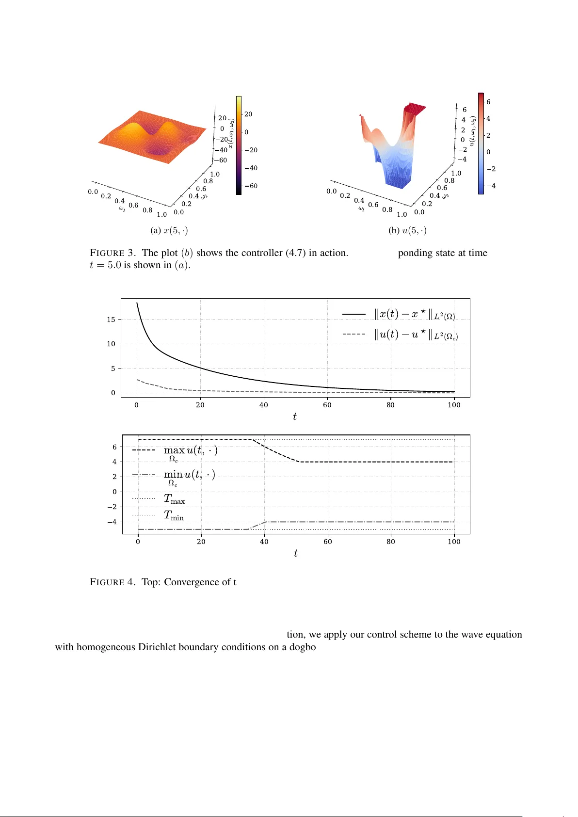
ST ABILIZA TION OF MONO TONE CONTR OL SYSTEMS WITH INPUT CONSTRAINTS TILL PREUSTER 1 , HANNES GERN ANDT 2 , AND MANUEL SCHALLER 1 A B S T R AC T . W e present a stabilizing output-feedback controller for nonlinear finite and infinite-dimensional con- trol systems governed by monotone operators that respects given input constraints. In particular , we show under a detectability-like assumption that a saturated version of the classical output feedback controller in passivity-based control achie ves control-constrained stabilization as long as the control corresponding to the desired equilibrium is in the interior of the control constraint set. W e illustrate our findings using a heat equation, a wave equation, and a finite-dimensional nonlinear port-Hamiltonian system. K eywords: stabilization, monotone operators, output feedback, control constraints 1. I N T RO D U C T I O N Maximal monotone operators pro vide a unifying frame work for the analysis of nonlinear and infinite-dimensional dynamical systems. Originating in con vex analysis and nonlinear functional analysis, monotonicity has become a central structural property in the study of e v olution equations, v ariational inequalities, and optimization algo- rithms. In Hilbert spaces, maximally monotone operators generate nonlinear contraction semigroups and thus induce well-posed dissipativ e dynamics. This semigroup viewpoint makes it possible to treat broad classes of systems, including linear , nonlinear , and even set-v alued, in a single unified framework. In parallel, port-Hamiltonian and dissipativ e systems theory has established powerful tools for stabilization via colocated feedback. In particular , negati ve output feedback is known to inject damping and to preserve structural properties such as passi vity . In finite-dimensional linear settings, this mechanism guarantees as- ymptotic stability under standard controllability or detectability assumptions. Under a suitable detectability assumption, it was shown in [22] that the colocated feedback stabilizes finite-dimensional port-Hamiltonian systems in the absence of control constraints. Related feedback laws have also been studied in [15, 24], where they appear in the context of damping injection . Ho wev er , when control constraints are imposed, classical feedback laws typically violate admissibility conditions, and stability under constrained actuation becomes sig- nificantly more delicate. Usually , adding predictive capabilities to the controller alle viates this problem, such as in model predictiv e control (MPC; [11, 18]). Therein, the feedback is computed by means of a finite-horizon optimal control problem. While asymptotic stability under input and state constraints is well studied, the ev alu- ation of the MPC feedback law is computationally challenging because it implicitly requires solving a nonlinear optimization problem. The purpose of this work is to provide an easy-to-implement output-feedback controller that (i) satisfies giv en control constraints and (ii) achiev es asymptotic stability for nonlinear control systems. The class of problems we consider are maximal monotone contr ol systems with colocated input-output structure. Specifically , we consider systems of the form ˙ x ( t ) = − M ( x ( t )) + B u ( t ) , y ( t ) = B ∗ x ( t ) , where M is maximally monotone on a Hilbert space X and B is a bounded linear input operator with adjoint B ∗ . This class encompasses linear dissipati ve systems, nonlinear gradient-type flows, and finite and infinite- dimensional port-Hamiltonian models. The colocated output y = B ∗ x ensures a natural energy balance relation and allo ws for the interpretation of u and y as conjugate port v ariables. Our objectiv e is constrained stabilization to wards a prescribed controlled equilibrium ( x ⋆ , u ⋆ ) . Gi ven a closed input constraint set F ⊂ U , we seek an output feedback law that enforces u ( t ) ∈ F pointwise while 1 J U N I O R P R O F E S S O R S H I P N U M E R I C A L M A T H E M A T I C S , F AC U LT Y O F M AT H E M A T I C S , C H E M N I T Z U N I V E R S I T Y O F T E C H N O L - O G Y , G E R M A N Y , M A I L : { T I L L . P R E U S T E R , M A N U E L . S C H A L L E R } @ M ATH . T U - C H E M N I T Z . D E 2 S C H O O L O F M ATH E M AT I C S A N D N A T U R A L S C I E N C E S , U N I V E R S I T Y O F W U P P E RT A L , G E R M A N Y , M A I L : G E R N A N D T @ U N I - W U P P E RTAL . D E This work was funded by the Deutsche Forschungsgemeinschaft (DFG, German Research Foundation) – Project-ID 531152215 – CRC 1701. 1 2 ensuring asymptotic con ver gence x ( t ) → x ⋆ . Rather than employing dynamic compensation or optimization- based control, we in vestigate a structurally simple saturated static output feedback obtained by projecting the unconstrained damping injection onto F : u ( x ) = P F ( u ⋆ − B ∗ ( x − x ⋆ )) . The central insight of this paper is that monotonicity provides suf ficient dissipativity to guarantee con vergence under this projected feedback, even in nonlinear and infinite-dimensional settings. The projection operator acts as a cut-off to the classical damping injection to guarantee the satisfaction of control constraints. Our analysis sho ws that, under a suitable detectability assumption, the closed-loop operator remains maximally monotone and generates a nonlinear contraction semigroup with the desired equilibrium as its unique asymptotically stable point. The main contribution of this work is as follows. W e prov e that a projection-based saturated output feed- back enforces arbitrary closed input constraints containing the equilibrium input while achieving asymptotic stability of the closed-loop. W e illustrate the wide applicability of our results by numerical e xamples in volving a nonlinear finite-dimensional problem and problems subject to wa ve and heat equations. The paper is organized as follows. After recalling the basics of maximal monotone operators and nonlinear semigroups in Section 2, we provide our main analytical results in Section 3. Therein, we first introduce maximal monotone control systems, formulate the stabilization problem and analyze the projected feedback law , establish well-posedness of the closed-loop dynamics, and prove asymptotic con ver gence in our main result Theorem 3.7 of Subsection 3.1 under a vanishing output vanishing state (V O VS) condition. Then, in Subsection 3.2 we sho w that, for linear problems, this assumption is satisfied if the system is detectable. Last, in Section 4, we illustrate the controller by means of v arious examples. Code a vailability . The code for all numerical experiments is provided in the repository www.github.com/preustertill/saturated_output_feedback . 2. N O T A T I O N S A N D P R E L I M I N A R I E S Throughout this note, we let X and U be two Hilbert spaces. The inner product of X is denoted by ⟨· , ·⟩ X . The set of bounded linear operators from X to U is denoted by L ( X, U ) . W e call a (possibly unbounded, nonlinear) operator M : X ⊃ D ( M ) → X with domain D ( M ) monotone if ⟨ M ( x ) − M ( z ) , x − z ⟩ X ≥ 0 (2.1) for all x, z ∈ D ( M ) . If M does not admit a proper monotone extension then M is called maximal monotone . Equi valently , λI + M is onto for some (and hence for all) λ > 0 , [3]. T o av oid confusion, we denote the zeros of nonlinear monotone operators M : X ⊃ D ( M ) → X by zer( M ) = { x ∈ D ( M ) : M ( x ) = 0 } whereas the kernel of a linear operator A : X ⊃ D ( A ) → U is indicated by ker A . Since control systems by maximally monotone operators M are the main subject of this paper , we first consider the initial v alue problem d d t x ( t ) = − M ( x ( t )) + f ( t ) , x (0) = x 0 , (2.2) where f ∈ L 1 ((0 , ∞ ); X ) , i.e. f : (0 , ∞ ) → X is measurable and Bochner integrable. Define the nonlinear operator S ( t ) x 0 = lim n →∞  I + t n M  − n x 0 , x 0 ∈ D ( M ) . (2.3) It is well-kno wn, see [1, Definition 4.4], that the operator giv en in (2.3) defines a semigroup ( S ( t )) t ≥ 0 : D ( M ) → D ( M ) of nonlinear nonexpansi ve mappings, i.e. ∥ S ( t ) x − S ( t ) z ∥ X ≤ ∥ x − z ∥ X (2.4) for all t ≥ 0 , x, z ∈ D ( M ) . In this case, we say that the semigroup S ( t ) is generated by − M . In the homogeneous case, that is, f ≡ 0 , then for initial v alue x 0 ∈ D ( M ) the unique strong solution of (2.2) is gi ven by x ( t ) = S ( t ) x 0 , t ≥ 0 . (2.5) 3 If, more generally , x 0 ∈ D ( M ) , Equation (2.5) defines the unique mild solution of (2.2). In presence of an inhomogeneity f ∈ W 1 , 1 ((0 , ∞ ); X ) , the corresponding strong (and mild) solution exists, see e.g., [1, Thm. 4.5]. W e recall the following result from [27]. Let A : X ⊃ D ( A ) → X be a closed, densely defined, linear maximal monotone operator and let ( T ( t )) t ≥ 0 , be the semigroup generated by − A . Let B : X → X be a continuous, everywhere defined, nonlinear monotone operator . Then, for every x 0 ∈ X , there exists a unique solution P ( t ) x 0 of the integral equation P ( t ) x 0 = T ( t ) x 0 − Z t 0 T ( t − s ) B ( P ( s ) x 0 ) ds, t ≥ 0 . (2.6) Here, ( P ( t )) t ≥ 0 , is a strongly continuous semigroup of nonlinear nonexpansi ve mappings on X with generator − ( A + B ) , and A + B is maximal monotone in X . W e call (2.6) the variation-of-parameters formula . 3. C O N S T R A I N E D S TA B I L I Z AT I O N O F M O N O T O N E C O N T R O L S Y S T E M S The class of systems considered in this work is governed by a maximally monotone operator together with a linear , bounded input operator . W e further assume a particular structure of the output equation, namely we assume a colocated input-output configuration. In this sense, our setting comprises many models from port- Hamiltonian theory (see, e.g., [13, 25]). Definition 1. Let X and U be Hilbert spaces. Let M : X ⊃ D ( M ) → X be a maximally monotone operator , and let B ∈ L ( U, X ) . Then we call d d t x ( t ) = − M ( x ( t )) + B u ( t ) , x (0) = x 0 , (3.1a) y ( t ) = B ∗ x ( t ) (3.1b) a maximal monotone contr ol system, abbre viated by ( M , B ) . For finite-dimensional systems, the class (3.1) was introduced in [4]. In [9, 10], the class was extended to infinite-dimensional dynamics and set-valued operators to study optimization algorithms in volving inequality constraints and projection operators. W e now may formulate the contrib ution of this work mathematically precise. Problem formulation . Gi ven a maximally monotone control system in the sense of (3.1), a con ve x and closed control constraint set F ⊂ U and a prescribed controlled equilibrium ( x ⋆ , u ⋆ ) ∈ D ( M ) × int F , i.e., − M ( x ⋆ ) + B u ⋆ = 0 . (3.2) Then our goal is to find an output feedback law κ ( x ⋆ ,u ⋆ ) : U → U such that with u = κ ( x ⋆ ,u ⋆ ) ( B ∗ x ) ∈ F ⊂ U , the dynamics ˙ x = − M ( x ) + B u = − M ( x ) + B κ ( x ⋆ ,u ⋆ ) ( B ∗ x ) is asymptotically stable, i.e., x ( t ) → x ⋆ for t → ∞ . In this work, we will show that the easy-to-implement and conceptually simple saturated output injection feedback law u = κ ( x ⋆ ,u ⋆ ) ( y ) = P F ( u ⋆ − ( y − y ⋆ )) = P F ( u ⋆ − B ∗ ( x − x ⋆ )) (3.3) fulfills this task. Here, y ⋆ = B ∗ x ⋆ is the equilibrium output and P F is the U -orthogonal projection onto the closed set F ⊂ U . 3.1. Main result: Control-constrained stabilization. T o show that the feedback law (3.3) asymptotically stabilizes the the open-loop dynamics (3.1), we will analyze the closed-loop dynamics d d t x ( t ) = − M cl ( x ( t )) , x (0) = x 0 , (3.4a) y ( t ) = B ∗ x ( t ) (3.4b) gov erned by the operator M cl : X ⊃ D ( M ) → X with M cl ( x ) = M ( x ) − B P F ( u ⋆ − B ∗ ( x − x ⋆ )) . (3.5) Before sho wing asymptotic stability of (3.4), we show maximal monotonicity of the closed-loop operator M cl . T o deal with the nonlinear projection induced by the saturated feedback law , we start with an auxiliary result. 4 Lemma 3.1. Let F ⊂ U be closed and conve x. Then, it holds that P F is firmly nonexpansive , i.e., ⟨ P F ( x ) − P F ( z ) , x − z ⟩ U ≥ ∥ P F ( x ) − P F ( z ) ∥ 2 U (3.6) for all x, z ∈ U . Pr oof. W e define the indicator function i F : U → R ∪ { + ∞} via i F ( z ) = ( 0 , if z ∈ F , + ∞ , otherwise . By closedness and con ve xity of F ⊂ U , i F is a proper , con ve x and lower semi-continuous function. Thus, its subgradient ∂ i F : U ⇒ U defined by ∂ i F ( z 0 ) =  z ′ ∈ U   ⟨ z ′ , x − z 0 ⟩ U ≤ i F ( x ) − i F ( z 0 ) ∀ x ∈ U  is a set-valued maximal monotone operator , [3, Thm. 20.25]. By [3, Prop. 23.8], its resolvent ( I + ∂ i F ) − 1 is an ev erywhere defined, firmly nonexpansiv e operator . Furthermore, from [3, Ex. 12.25] we hav e that ( I + ∂ i F ) − 1 = P F which prov es the claim. □ The follo wing result sho ws that due to nonexpansitvity of the projection, the closed-loop system is governed by a maximal monotone operator . Lemma 3.2. The governing operator M cl : X ⊃ D ( M ) → X of the closed-loop system (3.4) is maximal monotone. Pr oof. W e first show that the operator K : X → X with K ( x ) : = − B P F ( u ⋆ − B ∗ ( x − x ⋆ )) is monotone. T o this end, let x, y ∈ X and set ˜ x : = x − x ⋆ , ˜ y : = y − x ⋆ . Then, monotonicity of K follows from ⟨− B P F ( u ⋆ − B ∗ ˜ x ) + B P F ( u ⋆ − B ∗ ˜ y ) , x − y ⟩ X = ⟨ P F ( u ⋆ − B ∗ ˜ x ) − P F ( u ⋆ − B ∗ ˜ y ) , − B ∗ ˜ x + B ∗ ˜ y ⟩ X ≥ ∥ P F ( u ⋆ − B ∗ ˜ x ) − P F ( u ⋆ − B ∗ ˜ y ) ∥ 2 X ≥ 0 , where the second-last inequality follows from P F being firmly nonexpansiv e, cf. Lemma 3.1. Because the sum of two monotone operators is monotone, we conclude that M cl = M + K is a monotone operator . The maximality of M cl is a consequence of D ( K ) = X and perturbation theory for maximal operators [3, Cor . 25.5]. □ The follo wing auxiliary result pro vides a relation of the desired steady state and the zeros of the closed-loop operator . Lemma 3.3. Let F ⊂ U be closed, conve x and let a contr olled steady state ( x ⋆ , u ⋆ ) ∈ D ( M ) × int F be given. Then, { x ⋆ } ⊂ zer( M cl ) ⊂ { x ⋆ } + ker B ∗ . (3.7) In particular , zer( M cl ) is nonempty . Pr oof. First, x ⋆ ∈ zer( M cl ) as M ( x ⋆ ) − B P F ( u ⋆ − B ∗ ( x ⋆ − x ⋆ )) = M ( x ⋆ ) − B P F ( u ⋆ ) = M ( x ⋆ ) − B u ⋆ = 0 due to u ⋆ ∈ in t F and since ( x ⋆ , u ⋆ ) is a controlled equilibrium of the open-loop system (3.1). T o see the second inclusion, let x ∈ zer( M cl ) , i.e., M ( x ) = B P F ( u ⋆ − B ∗ ( x − x ⋆ )) . Set ˜ x = x − x ⋆ . By monotonicity of M and as M ( x ⋆ ) = B u ⋆ we obtain 0 ≤ ⟨ M ( x ) − M ( x ⋆ ) , x − x ⋆ ⟩ X = ⟨ B P F ( u ⋆ − B ∗ ˜ x ) − B u ⋆ , ˜ x ⟩ X = −⟨ P F ( u ⋆ − B ∗ ˜ x ) − P F ( u ⋆ ) , u ⋆ − B ∗ ˜ x − u ⋆ ⟩ U ≤ −∥ P F ( u ⋆ − B ∗ ˜ x ) − u ⋆ ∥ 2 U 5 ≤ 0 where the second-last inequality follo ws from the non-expansi vity of P F prov en in Lemma 3.1. Hence, P F ( u ⋆ − B ∗ ( x − x ⋆ )) = u ⋆ ∈ int F such that B ∗ ( x − x ⋆ ) = 0 and hence x − x ⋆ ∈ ker B ∗ which prov es the assertion. □ The follo wing result thus directly follows. Corollary 3.4. The pair ( x ⋆ , 0) ∈ D ( M ) × U is an equilibrium of the closed-loop system (3.4) . Since (3.4) is governed by the operator M cl defined in (3.5), and as the latter is maximal monotone due to Lemma 3.2, there e xists a semigroup ( S cl ( t )) t ≥ 0 : D ( M ) → D ( M ) of nonlinear none xpansi ve mappings. The strong (and mild) solutions of (3.4) are gi ven by x ( t ) = S cl ( t ) x 0 t ≥ 0 . W e no w focus on the asymptotic behavior of the closed-loop semigroup S cl ( t ) . T o this end, we first recall a result from [26, Lem. A.9]. Lemma 3.5. Let W : X ⊃ D ( W ) → X be maximally monotone and ( T ( t )) t ≥ 0 be the semigr oup of nonlinear nonexpansive mappings on D ( W ) generated by − W . F or x ⋆ ∈ D ( W ) , the following ar e equivalent: (i) T ( t ) x ⋆ = x ⋆ for all t ≥ 0 ; (ii) x ⋆ ∈ zer( W ) . The preceding lemma shows that the set of fixed points of the semigroup associated with (3.4) coincides with the zero set of the gov erning operator M cl . Having established this con ver gence to an equilibrium we sho w under a detectability-like assumption, that this equilibrium coincides with the unique zero x ⋆ of M , see (3.2). V arious conditions guaranteeing con ver gence of nonlinear semigroups generated by dissipativ e operators hav e been established in the literature; see, for example, [7, 19]. In the present work, we employ a con vergence criterion due to [16], which provides a con venient tool for establishing strong con ver gence of trajectories. This is advantageous since classical LaSalle-type arguments typically require additional compactness assumptions, such as compactness of the resolvent or precompactness of trajectories [6]. For a maximally monotone operator W , we denote the projection of some x ∈ D ( W ) onto the (nonempty and closed) set zer( W ) by P x . For the reader’ s con venience, we recall the main result of [16]. Theorem 3.6. Let W : X ⊃ D ( W ) → X be maximally monotone and let ( T ( t )) t ≥ 0 be the semigr oup gener ated by − W . Assume that W satisfies: (i) zer( W )  = ∅ ; (ii) F or any x 0 ∈ D ( W ) and ( t n ) n ∈ N ⊂ [0 , ∞ ) with t n → ∞ for n → ∞ , the con verg ence lim n →∞ ⟨ W ( T ( t n ) x 0 ) , T ( t n ) x 0 − P T ( t n ) x 0 ⟩ X = 0 implies lim inf n →∞ dist( T ( t n ) x 0 , zer( W )) = 0 . Then, for every x 0 ∈ D ( W ) , the trajectory T ( t ) x 0 con ver ges as t → ∞ to a fixed point of ( T ( t )) t ≥ 0 in the sense of Lemma 3.5 (i). W e note that the previously stated theorem resembles a slight modification of [16, Theorem 2.1]. In its original version, the con ver gence condition (ii) has to be ensured for any bounded sequence ( x n ) n ∈ N that renders ( W ( x n )) n ∈ N bounded. Howe ver , as becomes clear when inspecting the proof of [16, Theorem 2.1], the weaker condition (ii) stated abo ve utilizing sequences emer ging from trajectory samples is sufficient. W e now state the main result of this paper . Besides monotonicity of the gov erning main operator , the main ingredient is the follo wing detectability-like property . Definition 2. W e say that the maximally monotone system ( M , B ) given by (3.1) with ( S ( t )) t ≥ 0 being the nonlinear semigr oup generated by − M fulfills the vanishing output vanishing state (V O VS) pr operty at x ⋆ if for all x 0 ∈ D ( M ) lim t →∞ B ∗ ( S ( t ) x 0 − x ⋆ ) = 0 implies lim t →∞ S ( t ) x 0 = x ⋆ . 6 In the subsequent Subsection 3.2, we sho w that for linear systems, this condition is implied by detectability . The next result shows that the proposed saturated feedback law is asymptotically stabilizing when assuming the V O VS property for the closed-loop system. Theorem 3.7. Let F ⊂ U be closed, con ve x and let a contr olled steady state ( x ⋆ , u ⋆ ) ∈ D ( M ) × in t F be given. Further , let the system (3.4) fulfill the VO VS pr operty at x ⋆ . Let ( S cl ( t )) t ≥ 0 be the semigr oup generated by − M cl as in (3.5) . Then, for all x 0 ∈ D ( M ) , S cl ( t ) x 0 → x ⋆ as t → ∞ . Pr oof. The proof strategy is to verify the conditions of Theorem 3.6 for W = M cl . As x ⋆ ∈ zer( M cl ) due to Lemma 3.3, condition (i) is satisfied. Thus, we remain to v erify the condition (ii). T o this end, in a first step we verify that the con vergence condition (ii) of Theorem 3.6 is satisfied for the maximal monotone operator M cl defined in (3.5). In a second step, we use the V O VS property of (3.4) at x ⋆ to show that the strong limit of the semigroup ( S cl ( t )) t ≥ 0 coincides with the unique equilibrium x ⋆ ∈ zer( M cl ) , cf. (3.2). Let P be the projection onto zer( M cl ) : = { x ∈ D ( M ) : M ( x ) = B P F ( u ⋆ − B ∗ ( x − x ⋆ )) } . Let x 0 ∈ D ( M ) , ( t n ) n ∈ N ⊂ [0 , ∞ ) with t n → ∞ for n → ∞ , and denote x n := S ( t n ) x 0 ⊂ D ( M ) . Assume that the condition of Theorem 3.6 (ii) holds, that is, ⟨ M cl ( x n ) , x n − P x n ⟩ → 0 as n → ∞ . (3.8) Due to the second inclusion of (3.7) of Lemma 3.3, v n := P x n − x ⋆ ∈ ker B ∗ for each n ∈ N . Along the lines of the proof of Lemma 3.3, we set ˜ x n = x n − x ⋆ and we obtain ⟨ M cl ( x n ) , x n − P x n ⟩ X = ⟨ M cl ( x n ) − M cl ( P x n ) , x n − P x n ⟩ X = ⟨ M ( x n ) − M ( x ⋆ + v n ) , x n − ( x ⋆ + v n ) ⟩ X + ⟨− B P F ( u ⋆ − B ∗ ˜ x ) + B P F ( u ⋆ − B ∗ v n ) , x n − ( x ⋆ + v n ) ⟩ X ≥ ⟨ P F ( u ⋆ − B ∗ ˜ x ) − P F ( u ⋆ ) , − B ∗ x n − ( − B ∗ ( x ⋆ + v n )) ⟩ U = ⟨ P F ( u ⋆ − B ∗ ( x n − x ⋆ )) − P F ( u ⋆ ) , − B ∗ ( x n − x ⋆ ) ⟩ U ≥ ∥ P F ( u ⋆ − B ∗ ( x n − x ⋆ )) − u ⋆ ∥ 2 U where we used Lemma 3.1 in the last inequality . Thus, due to (3.8), p n := P F ( u ⋆ − B ∗ ( x n − x ⋆ )) → u ⋆ as n → ∞ . Since u ⋆ ∈ int F , there exists an r > 0 such that the open ball B r ( u ⋆ ) ⊂ F . Hence, for sufficiently large n ∈ N we hav e p n ∈ B r ( u ⋆ ) ⊂ F . (3.9) Hence, for n ∈ N lar ge enough, p n ∈ F such that p n = P F ( u ⋆ − B ∗ ( x n − x ⋆ )) = u ⋆ − B ∗ ( x n − x ⋆ ) and thus due to p n → u ⋆ and resubstituting x n = S cl ( t n ) x 0 , B ∗ ( S cl ( t n ) x 0 − x ⋆ ) → 0 as n → ∞ . Then, the assumed V O VS property of (3.4) at x ⋆ yields lim n →∞ S cl ( t n ) x 0 = x ⋆ ∈ zer( M cl ) (3.10) which prov es the condition (ii) of Theorem 3.6. Hence, S cl ( t ) x 0 con ver ges strongly to a fixed point of the semigroup. T o see that this fixed point is indeed also the limit of the sampled trajectory (3.10), let n ∈ N and t ≥ t n . Then ∥ S cl ( t ) x 0 − x ⋆ ∥ = ∥ S cl ( t n + ( t − t n )) x 0 − x ⋆ ∥ = ∥ S cl ( t − t n ) S cl ( t n ) x 0 − S cl ( t − t n ) x ⋆ ∥ ≤ ∥ S cl ( t n ) x 0 − x ⋆ ∥ , where in the last inequality we used the none xpansi vity of the semigroup (2.4). This sho ws that S cl ( t ) x 0 → x ⋆ for t → ∞ . □ 7 3.2. Detectability and the V O VS property. In this part, we relate the V O VS property to detectability . W e sho w suf ficient conditions for the VO VS property being the central assumption of our main result Theorem 3.7 in the particular case of linear control systems. W e note that, ev en in this case, the results proving asymptotic stability with the suggested output feedback subject to control constraints is novel. W e note that, e ven for linear systems, the saturated feedback leads to a nonlinear closed-loop system. By [6, Def. 8.1.1], a linear control system ( A, B ) = ( A, B , B ∗ ) is exponentially detectable if there exists L ∈ L ( U, X ) such that − A + LB ∗ generates an exponentially stable semigroup ( T − A + LB ∗ ( t )) t ≥ 0 , i.e., ∥ T − A + LB ∗ ( t ) ∥ ≤ ce − ω t , t ≥ 0 , for some c ≥ 1 , ω > 0 . Note that, by linearity of A , the property of ( A, B ) being exponentially detectable is independent of the controlled equilibrium. The following Proposition 3.8 shows that for linear systems, detectability implies the V O VS notion for the open-loop system. Then, in the subsequent Proposition 3.9, we show that this also implies V O VS for the nonlinear closed-loop system. Proposition 3.8. Let ( A, B ) be a maximal monotone contr ol system where A : X ⊃ D ( A ) → X is a linear operator and let ( x ⋆ , u ⋆ ) be a contr olled equilibrium of ( A, B ) . If ( A, B ) is e xponentially detectable, then ( A, B ) fulfills the V O VS pr operty at x ⋆ . Pr oof. The first part of the proof adapts the argument of [14, Proposition 2.6] to the infinite-dimensional set- ting. By exponential detectability of ( A, B ) , there exists L ∈ L ( U, X ) such that − A + LB ∗ generates an exponentially stable semigroup ( T − A + LB ∗ ( t )) t ≥ 0 . Define the shifted variables x s ( t ) : = x ( t ) − x ⋆ , u s ( t ) : = u ( t ) − u ⋆ , y s ( t ) : = y ( t ) − y ⋆ . Define the observer -type system d d t x s ( t ) = − Ax s ( t ) = − Ax s ( t ) + L ( B ∗ x s ( t ) − y s ( t )) . (3.11) For a fixed x s, 0 = x 0 − x ⋆ ∈ D ( A ) , the solution x s ( t ) = S s ( t ) x s, 0 of (3.11) satisfies the variation-of-parameters formula (2.6), that is, S s ( t ) x s, 0 = T − A + LB ∗ ( t ) x s, 0 − Z t 0 T − A + LB ∗ ( t − s )( Ly s ( s )) d s. For bre vity , we write ∥ x s, 0 ∥ X = ∥ x s, 0 ∥ and ∥ L ∥ L ( U,X ) = ∥ L ∥ . T aking norms and using exponential decay of T − A + LB ∗ ( t ) , we get ∥ S s ( t ) x s, 0 ∥ ≤ ce − ω t ∥ x s, 0 ∥ + Z t 0 ce − ω ( t − s ) ∥ L ∥∥ y s ( s ) ∥ d s ≤ ce − ω t ∥ x s, 0 ∥ + c ∥ L ∥∥ y s ∥ L ∞ (0 ,t ; U ) Z t 0 e − ω ( t − s ) d s, for some c ≥ 1 , ω > 0 . Since R t 0 e − ω ( t − s ) = 1 − e − ωt ω ≤ 1 ω , ∥ S s ( t ) x s, 0 ∥ ≤ ce − ω t ∥ x s, 0 ∥ + c ∥ L ∥ ω ∥ y s ∥ L ∞ (0 ,t ; U ) . Consequently , the system (3.11), and with that also system ( A, B ) , is output-to-state stable (OSS) in the sense of [5, Def. 2.2], see also [21]. It follows from [5, Cor . 4.8], that ( A, B ) satisfies the V O VS property at the origin. Howe ver , from S s ( t ) x s, 0 = S ( t ) x 0 − x ⋆ , y s ( t ) = y ( t ) − y ⋆ , we conclude that ( A, B ) satisfies the V O VS property at x ⋆ . □ W e now show that, for linear control systems ( A, B ) , exponential detectability is sufficient to ensure that the closed-loop system ( A cl , B ) satisfies the V O VS property at x ⋆ . In particular, exponential detectability guarantees that the assumptions of Theorem 3.7 are met. Proposition 3.9. Let ( A, B ) be a maximal monotone contr ol system where A : X ⊃ D ( A ) → X is a linear operator and let ( x ⋆ , u ⋆ ) be a contr olled equilibrium of ( A, B ) . If ( A, B ) is exponentially detectable, the nonlinear closed-loop system ( A cl , B ) with A cl ( x ) = Ax − B P F ( u ⋆ − B ∗ ( x − x ⋆ )) fulfills the VO VS pr operty at x ⋆ . 8 Pr oof. Exponential detectability of ( A, B ) yields the existence of L ∈ L ( U, X ) such that − A + LB ∗ generates an exponentially stable semigroup ( T − A + LB ∗ ( t )) t ≥ 0 . Similar to the proof of Proposition 3.8 and shifting the system, we define A cl ,s ( x s ) = A cl ( x s + x ⋆ ) − A cl ( x ⋆ ) and the corresponding observer system d d t x s ( t ) = − A cl ,s x s ( t ) (3.12) = − A cl ,s x s ( t ) + L ( B ∗ x s ( t ) − B ∗ x s ( t )) = − Ax s ( t ) + f s ( x s ( t )) + L ( B ∗ x s ( t ) − y s ( t )) = ( − A + LB ∗ ) x s ( t ) + f s ( x s ( t )) − Ly s ( t ) where f s ( x s ) = f ( x s + x ⋆ ) − f ( x ⋆ ) with f ( x ) = B P F ( u ⋆ − B ∗ ( x − x ⋆ ) . Similar to the proof Proposition 3.8, we now show that this system is OSS in the sense of [5, Def. 2.2], see also [21]. T o this end, observe that Lemma 3.1 yields ∥ P F ( v ) − P F ( w ) ∥ 2 U ≤ ⟨ P F ( v ) − P F ( w ) , v − w ⟩ U ≤ ∥ P F ( v ) − P F ( w ) ∥ U ∥ v − w ∥ U which implies ∥ P F ( v ) − P F ( w ) ∥ U ≤ ∥ v − w ∥ U for all v , w ∈ U . Thus, f s is Lipschitz continuous. T o see this, let ˜ x, ˜ z ∈ X and set x = ˜ x + x ⋆ , z = ˜ z + x ⋆ , ∥ f s ( ˜ x ) − f s ( ˜ z ) ∥ X = ∥ f ( x ) − f ( z ) ∥ X = ∥ B κ ( x ⋆ ,u ⋆ ) ( B ∗ x ) − B κ ( x ⋆ ,u ⋆ ) ( B ∗ z ) ∥ X ≤ ∥ B ∥ L ( U,X ) ∥ κ ( x ⋆ ,u ⋆ ) ( B ∗ x ) − κ ( x ⋆ ,u ⋆ ) ( B ∗ z ) ∥ U = ∥ B ∥ L ( U,X ) ∥ P F ( u ⋆ − B ∗ ˜ x ) − P F ( u ⋆ − B ∗ ˜ z ) ∥ U ≤ ∥ B ∥ L ( U,X ) ∥ B ∗ ˜ x − B ∗ ˜ z ∥ U ≤ ∥ B ∥ L ( U,X ) ∥ B ∗ ∥ L ( X,U ) ∥ x − z ∥ X = ∥ B ∥ L ( U,X ) ∥ B ∗ ∥ L ( X,U ) ∥ ˜ x − ˜ z ∥ X for all x, z ∈ X . Moreover , ∥ f s ( x s ) ∥ X = ∥ f ( x s + x ⋆ ) − f ( x ⋆ ) ∥ X ≤ ∥ B ∥ L ( U,X ) ∥ P F ( u ⋆ − B ∗ x s ) − P F ( u ⋆ ) ∥ U ≤ ∥ B ∥ L ( U,X ) ∥ u ⋆ − B ∗ x s − u ⋆ ∥ U = ∥ B ∥ L ( U,X ) ∥ y s ∥ U for all x s ∈ X . Again, for a fixed x s, 0 = x 0 − x ⋆ ∈ D ( A ) , the solution x s ( t ) = S cl ,s ( t ) x s, 0 of (3.4a) is the solution of (3.12) and the v ariation-of-parameters formula (2.6) giv es S cl ,s ( t ) x s, 0 = T − A + LB ∗ ( t ) x s, 0 + Z t 0 T − A + LB ∗ ( t − s )( f s ( S cl ,s ( t ) x s, 0 ) − Ly s ( s )) d s. Along the lines of the proof of Proposition 3.8, we combine exponential stabilty of ( T − A + LB ∗ ( t )) t ≥ 0 and the bound on f s ( x s ) to get ∥ S cl ,s ( t ) x s, 0 ∥ ≤ ce − ω t ∥ x s, 0 ∥ + c ( ∥ B ∥ + ∥ L ∥ ) ω ∥ y s ∥ L ∞ (0 ,t ; U ) . Thus, (3.12) is OSS and the same ar gumentation as in the end of the proof of Proposition 3.8 yields the claimed V O VS property . □ The pre vious proposition shows that for linear control systems, exponential detectability of the open-loop system implies the V O VS property of the closed-loop system. For nonlinear system, this implication is, to the best of the authors’ knowledge, an open problem. Howe ver , we show that for nonlinear systems, detectability as defined in [12] is at least equiv alent for the open and closed-loop system, respectiv ely . In [12], detectability (as usually) is defined for the origin. Here, in view of shifted passivity of our system, we will first define it for a general controlled steady state and then explain the correspondence to its shifted counterpart afterwards. 9 Definition 3. Let ( M , B ) be a maximal monotone contr ol system and let ( x ⋆ , u ⋆ ) ∈ D ( M ) × U be a contr olled equilibrium. Let S ( t ) be the semigr oup generated by − M . W e define the set of unobservable states on [0 , t ] at x ⋆ for t ≥ 0 by N ( M ,B ) x ⋆ ( t ) : = { x 0 ∈ D ( M ) : B ∗ S ( s ) x 0 = B ∗ x ⋆ ∀ s ∈ [0 , t ] } . The unobservable set at x ⋆ is then N ( M ,B ) x ⋆ : = ∩ t ≥ 0 N ( M ,B ) x ⋆ ( t ) . The maximal monotone contr ol system ( M , B ) is detectable at x ⋆ if lim t →∞ S ( t ) x 0 = x ⋆ for all x 0 ∈ N ( M ,B ) x ⋆ . W e briefly comment on the detectability notion from Definition 3 and its relation to other notions from the literature. Remark 1. Let a maximal monotone contr ol system ( M , B ) with contr olled equilibrium ( x ⋆ , u ⋆ ) ∈ D ( M ) × U be given. Define the shifted variables x s ( t ) : = x ( t ) − x ⋆ , u s ( t ) : = u ( t ) − u ⋆ , y s ( t ) : = y ( t ) − y ⋆ and the shifted operator M s : X ⊃ D ( M s ) = : D ( M ) − { x ⋆ } → X by M s ( x s ) : = M ( x s + x ⋆ ) − M ( x ⋆ ) . (3.13) By definition of ( x s , u s , y s ) , the shifted contr ol system is d d t x s ( t ) = − M s ( x s ( t )) + B u s ( t ) , (3.14a) y s ( t ) = B ∗ x s ( t ) (3.14b) with initial value x s (0) = x 0 − x ⋆ = : x s, 0 . It is immediate fr om the (3.13) that (3.14) again defines a maximal monotone contr ol system with contr olled equilibrium (0 , 0) . It is now easy to see that ( M , B ) is detectable at x ⋆ in the sense of Definition 3 if ( M s , B ) is detectable (at 0 ) in the sense of [12, Def. 10.7.3]. T o this end, let the semigr oup generated by − M be denoted by ( S ( t )) t ≥ 0 . Then S s ( t ) x s, 0 = S ( t ) x 0 − x ⋆ = S ( t )( x s, 0 + x ⋆ ) − x ⋆ defines the semigr oup generated by − M s . Thus, N ( M s ,B ) 0 = N ( M ,B ) x ⋆ − { x ⋆ } . (3.15) The following result shows that detectability holds for the open-loop system if and only if it holds for the closed-loop system resulting from application of our saturated output feedback. Proposition 3.10. Let F ⊂ U be closed, con vex and let a contr olled steady state ( x ⋆ , u ⋆ ) ∈ D ( M ) × int F be given. The maximal monotone contr ol system ( M , B ) is detectable at x ⋆ if and only if ( M cl , B ) is detectable at x ⋆ , wher e M cl is defined as in (3.5) . Pr oof. W e set M s ( x s ) = M ( x s + x ⋆ ) − M ( x ⋆ ) and M cl ,s ( x s ) = M cl ( x s + x ⋆ ) − M cl ( x ⋆ ) = M ( x s + x ⋆ ) − M ( x ⋆ ) − ( B P F ( u ⋆ − B ∗ x s ) − B u ⋆ ) = M s ( x s ) − ( B P F ( u ⋆ − B ∗ x s ) − B u ⋆ ) . Let ( S s ( t )) t ≥ 0 , ( S cl ,s ( t )) t ≥ 0 be the nonlinear semigroups generated by − M s and − M cl ,s , respecti vely . Then, d d t S s ( t ) x s, 0 = − M s ( S s ( t ) x s, 0 ) with initial value x s, 0 ∈ N ( M s ,B ) 0 . Furthermore, for initial values x s, 0 ∈ N ( M cl ,s ,B ) 0 (which, by definition, satisfy B ∗ S cl ,s ( t ) x s, 0 = 0 for all t ≥ 0 ), d d t S cl ,s ( t ) x s, 0 = − M cl ,s ( S cl ,s ( t ) x s, 0 ) 10 = − M s ( S cl ,s ( t ) x s, 0 ) − B ( P F ( u ⋆ − B ∗ S cl ,s ( t ) x s, 0 ) − u ⋆ ) = − M s ( S cl ,s ( t ) x s, 0 ) − B ( P F ( u ⋆ ) − u ⋆ ) = − M s ( S cl ,s ( t ) x s, 0 ) since u ⋆ ∈ int F . By uniqueness of strong solutions, we have lim t →∞ S s ( t ) x s, 0 = 0 for all x s, 0 ∈ N ( M s ,B ) 0 , if and only if, lim t →∞ S cl ,s ( t ) x s, 0 = 0 for all x s, 0 ∈ N ( M cl ,s ,B ) 0 , which prov es the claim. □ 4. N U M E R I C A L E X A M P L E S In this part, we provide three examples that highlight the applicabiltiy to our result to a wide range of problems. In particular , we consider a finite-dimensional nonlinear system in Subsection 4.1, a heat equation in 4.2 and a wa ve equation in Subsection 4.3. 4.1. A finite-dimensional example. W e consider the nonlinear problem ˙ x ( t ) = −∇ Ψ( x ( t )) +  0 − 1 1 0  ( x ( t ) − x ⋆ ) + [ 1 0 ] u ( t ) (4.1a) y ( t ) = [ 1 0 ] x ( t ) . (4.1b) where x ⋆ ∈ R 2 , Ψ : R 2 → R with Ψ( x ) = εg ( ∥ x − x ⋆ ∥ 2 ) with ε > 0 and g ( r ) = √ 1 + r such that ∇ Ψ( x ) = ε √ 1+ ∥ x − x ⋆ ∥ 2 ( x − x ⋆ ) . Note that the function Ψ is conv ex as Ψ( x ) = ε p 1 + ∥ x − x ⋆ ∥ 2 = ε   (1 , x − x ⋆ )   R 3 , such that Ψ is the composition of a conv ex function with an af fine mapping and hence con vex. Define the operator M : R 2 → R 2 corresponding to the autonomous part of (4.1) as M ( x ) = ∇ Ψ( x ) +  0 1 − 1 0  ( x − x ⋆ ) . Proposition 4.1. The operator M : R 2 → R 2 is maximal monotone and has its unique zer o at x ⋆ . Pr oof. Let J : =  0 1 − 1 0  . Then, for x, y ∈ R n : ⟨ M ( x ) − M ( y ) , x − y ⟩ R 2 = ⟨∇ Ψ( x ) − Ψ( y ) , x − y ⟩ R 2 + ⟨ J ( x − y ) , x − y ⟩ R 2 = ⟨∇ Ψ( x ) − ∇ Ψ( y ) , x − y ⟩ R 2 ≥ 0 , where the last inequality follows from the fact that gradients of proper, con ve x and lower semi-continuous functions are (maximal) monotone, [3, Thm. 20.25]. Hence, M is monotone and the maximality follows from M being ev erywhere defined. T o see that zer( M ) = { x ∗ } , let x ∈ zer( M ) , then 0 = ⟨ M ( x ) , x − x ⋆ ⟩ R 2 = ε ∥ x − x ⋆ ∥ 2 R 2 1 q 1+ ∥ x − x ⋆ ∥ 2 R 2 which prov es that x = x ⋆ . □ It is a direct consequence from Proposition 4.1 that ( x ⋆ , 0) defines a controlled equilibrium of (4.1). W e restrict the admissible controls to take v alues pointwise in the closed interv al F = [ a, b ] , a < 0 < b. Clearly , F is conv ex, closed and u ⋆ = 0 ∈ in t F . The corresponding output feedback law (3.3) is u ( t ) = P F ( − [ 1 0 ] ( x ( t ) − x ⋆ ) = P [ a,b ] ( − ( x 1 ( t ) − x ⋆ 1 )) . Thus, the closed-loop system is gi ven by d d t x ( t ) = − M ( x ( t )) + h P [ a,b ] ( − ( x 1 ( t ) − x ⋆ 1 )) 0 i (4.2a) y ( t ) = x 1 ( t ) (4.2b) 11 The following result shows that the example satisfies the assumptions of the asymptotic stability result Theo- rem 3.7. Proposition 4.2. The system (4.2) fulfills the VO VS pr operty at x ⋆ . Pr oof. W e observe that V ( x ) : = 1 2 ∥ x − x ⋆ ∥ 2 R 2 defines a L yapunov function for (4.2). Precisely , let z = x − x ⋆ and consider ˙ V ( x ) = ⟨∇ V ( x ) , − M ( x ) + h P [ a,b ] ( − ( x 1 − x ⋆ 1 )) 0 i ⟩ R 2 = − ε ∥ z ∥ 2 R 2 q 1+ ∥ z ∥ 2 R 2 + z 1 P [ a,b ] ( − z 1 ) ≤ 0 . Moreov er , the computations in the proof of Proposition 4.1 yield that S : = n x ∈ R 2 : ˙ V ( x ) = 0 o = { x ⋆ } . By [20, Lem. 5.7.8], (4.2) is globally asymptotically stable and hence, fulfills the V O VS property at x ⋆ . □ A combination of Proposition 4.2 and Theorem 3.7 proves that the suggested controller (3.3) asymptotically stabilizes the system (4.1a). The numerical results are illustrated in Figure 1 for the choices x ⋆ = ( − 1 . 0 , 1 . 5) , a = − 0 . 7 , b = 0 . 9 , x 0 = (2 . 0 , − 3 . 0) and ε = 0 . 01 . F I G U R E 1 . T op: Closed-loop state trajectories x 1 ( t ) , x 2 ( t ) of (4.2a) with initial value x 0 = (2 . 0 , − 3 . 0) . Bottom: Saturated control input u ( t ) = P [ a,b ] ( − ( x 1 ( t ) − x ⋆ 1 )) . 4.2. T wo-dimensional heat equation. W e define the bounded Lipschitz domain Ω : = (0 , 1) × (0 , 1) . The Neu- mann trace ∂ ν x of x ∈ H 2 (Ω) is defined by the unique element w ∈ H − 1 / 2 ( ∂ Ω) that fulfills the integration- by-parts formula ⟨∇ x, ∇ y ⟩ L 2 (Ω; R 2 ) = ⟨− ∆ x, y ⟩ L 2 (Ω) + ⟨ w , y | ∂ Ω ⟩ H − 1 / 2 ( ∂ Ω) ,H 1 / 2 ( ∂ Ω) (4.3) for all y ∈ H 1 (Ω) . The Neumann Laplacian is then gi ven by the operator A N : L 2 (Ω) ⊂ D ( A N ) → L 2 (Ω) with D ( A N ) = { x ∈ H 2 (Ω) : ∂ ν x = 0 } , A N x = − ∆ x. 12 It follo ws directly from (4.3) that the Neumann Laplacian is monotone, i.e., ⟨ A N x, x ⟩ L 2 (Ω) = ∥∇ x ∥ 2 L 2 (Ω; R 2 ) ≥ 0 ∀ x ∈ D ( A N ) , (4.4) and it is clear that A N is self-adjoint and hence maximal with respect to this property . Let Ω c ⊂ Ω denote the subregion on which a distributed heating/cooling source is applied. W e assume that Ω c has positiv e Lebesgue measure | Ω c | > 0 . W e define the bounded linear operator B : L 2 (Ω c ) → L 2 (Ω) by extension by zero, i.e., ( B u )( ω ) : = ( 1 Ω c u )( ω ) : = ( u ( ω ) , if ω ∈ Ω c ; 0 , otherwise . Its adjoint B ∗ : L 2 (Ω) → L 2 (Ω c ) is given by the restriction B ∗ x = x | Ω c . Consequently , d d t x ( t ) = − A N ( x ( t )) + 1 Ω c u ( t ) , x (0) = x 0 , (4.5a) y ( t ) = x ( t ) | Ω c (4.5b) defines a maximal monotone control system (3.1). Assuming that the distributed heating/cooling source is constrained to [ T min , T max ] ∋ 0 we define the control constraint set F =  u ∈ L 2 (Ω c ) : T min ≤ u ( ω ) ≤ T max a.e. in Ω c  . W e prescribe a steady distributed input u ⋆ supported in Ω c by u ⋆ ( x, y ) = ( 4 sin  2 π ξ ( x )  sin  2 π η ( y )  , ( x, y ) ∈ Ω c , 0 , ( x, y ) / ∈ Ω c , where ξ ( x ) = x − 0 . 2 0 . 6 and η ( y ) = y − 0 . 2 0 . 6 . The amplitude is chosen such that T min ≤ u ⋆ ≤ T max and R Ω u ⋆ = 0 , ensuring compatibility with the Neumann Laplacian. The corresponding steady temperature profile x ⋆ is defined as the solution of the elliptic problem ∆ x ⋆ = − B u ⋆ in Ω , ∂ ν x ⋆ = 0 on ∂ Ω , Z Ω x ⋆ = 0 . (4.6) Since B u ⋆ v anishes outside Ω c , it follo ws that ∆ x ⋆ = 0 in Ω \ Ω c , so x ⋆ is harmonic outside the control region and nonconstant inside. The pair ( x ⋆ , u ⋆ ) is illustrated in Figure 2. 0.0 0.2 0.4 0.6 0.8 1.0 ω 1 0.0 0.2 0.4 0.6 0.8 1.0 ω 2 60 40 20 0 20 x ( ω 1 , ω 2 ) 60 40 20 0 20 (a) x ⋆ 0.0 0.2 0.4 0.6 0.8 1.0 ω 1 0.0 0.2 0.4 0.6 0.8 1.0 ω 2 4 2 0 2 4 6 u ( ω 1 , ω 2 ) 4 2 0 2 4 6 (b) u ⋆ F I G U R E 2 . The controlled equilibrium ( x ⋆ , u ⋆ ) with Ω c = (0 . 2 , 0 . 8) 2 . The saturated output feedback (3.3) is gi ven by u = κ x ⋆ ( y ) = P F ( u ⋆ − ( x − x ⋆ ) | Ω c ) (4.7) leading to the corresponding closed-loop system d d t x ( t ) = − A N , cl ( x ( t )) , (4.8a) 13 y ( t ) = x ( t ) | Ω c (4.8b) where A N , cl : L 2 (Ω) ⊃ D ( A N ) → L 2 (Ω) enjoys A N , cl ( x ) = A N x − 1 Ω c P F ( u ⋆ − ( x − x ⋆ ) | Ω c ) . The follo wing result shows that this system satisfies the assumptions of our stability result Theorem 3.7. Proposition 4.3. The system (4.8) fulfills the VO VS pr operty at x ⋆ . Pr oof. By Proposition 3.9, it is enough to prov e that ( A N , B ) is exponentially detectable. T o this end, we sho w that − ( A N + B B ∗ ) is the generator of an exponentially stable semigroup on L 2 (Ω) . T o see this, we prove coerci vity of A N + B B ∗ , i.e., we sho w that there exists a constant α > 0 such that ⟨ ( A N + B B ∗ ) x, x ⟩ L 2 (Ω) ≥ α ∥ x ∥ 2 L 2 (Ω) for all x ∈ D ( A N ) . By P oincar ´ e’ s inequality , [8, Ch. 5.8.1, Thm. 1], there exists a constant C > 0 such that ⟨ A N x, x ⟩ L 2 (Ω) = ∥∇ x ∥ 2 L 2 (Ω; R 2 ) ≥ C ∥ x − x ∥ 2 L 2 (Ω) (4.9) for all x ∈ D ( A N ) , where x : = R Ω x ( ω ) d ω denotes the avera ge of x over Ω . It follows from straightforward computations that for a, b ∈ R : | a + b | 2 ≥ 1 2 | a | 2 − 2 | b | 2 . (4.10) Thus, ∥ B ∗ x ∥ 2 L 2 (Ω) = Z Ω c | x ( ω ) | 2 d ω = Z Ω c | x + ( x ( ω ) − x ) | 2 d ω (4.10) ≥ Z Ω c 1 2 | x | 2 d ω − Z Ω c 2 | ( x ( ω ) − x ) | 2 d ω ≥ 1 2 | x | 2 | Ω c | − 2 ∥ x − x ∥ 2 L 2 (Ω) (4.10) ≥ 1 2 | x | 2 | Ω c | − 2 C ⟨ A N x, x ⟩ L 2 (Ω) for all x ∈ D ( A N ) . Hence, ⟨ ( A N + B B ∗ ) x, x ⟩ L 2 (Ω) = ⟨ A N x, x ⟩ L 2 (Ω) + ∥ B ∗ x ∥ 2 L 2 (Ω) ≥ | Ω c | 4(1+2 /C ) | x | 2 + C 2 ∥ x − x ∥ 2 L 2 (Ω) ≥ min( | Ω c | 4(1+2 /C ) , C 2 )( | x | 2 + ∥ x − x ∥ 2 L 2 (Ω) ) = min( | Ω c | 4(1+2 /C ) , C 2 ) ∥ x ∥ 2 L 2 (Ω) , where the last equality follo ws from ∥ x ∥ 2 L 2 (Ω) = ∥ x + ( x − x ) ∥ 2 L 2 (Ω) = ∥ x ∥ 2 L 2 (Ω) + 2 ⟨ x, x − x ⟩ L 2 (Ω) + ∥ x − x ∥ 2 L 2 (Ω) = | x | 2 + ∥ x − x ∥ 2 L 2 (Ω) . The desired result follows with α : = min( | Ω c | 4(1+2 /C ) , C 2 ) , which is positiv e due to the positi ve Lebesgue measure of the control region Ω c . □ The con ver gence of our suggested control scheme is visualized in the Figures 4 for for the choice T min = − 5 . 0 , T max = 7 . 0 . W e provide a snapshot of the saturated control with corresponding state at time t = 5 . 0 in Figure 3. 14 0.0 0.2 0.4 0.6 0.8 1.0 ω 1 0.0 0.2 0.4 0.6 0.8 1.0 ω 2 60 40 20 0 20 x ( t , ω 1 , ω 2 ) 60 40 20 0 20 (a) x (5 , · ) 0.0 0.2 0.4 0.6 0.8 1.0 ω 1 0.0 0.2 0.4 0.6 0.8 1.0 ω 2 4 2 0 2 4 6 u ( t , ω 1 , ω 2 ) 4 2 0 2 4 6 (b) u (5 , · ) F I G U R E 3 . The plot ( b ) shows the controller (4.7) in action. The corresponding state at time t = 5 . 0 is sho wn in ( a ) . 0 20 40 60 80 100 t 0 5 10 15 k x ( t ) − x k L 2 ( Ω ) k u ( t ) − u k L 2 ( Ω c ) 0 20 40 60 80 100 t 4 2 0 2 4 6 m a x Ω c u ( t , · ) m i n Ω c u ( t , · ) T m a x T m i n F I G U R E 4 . T op: Con ver gence of the closed-loop state and control. Bottom: Feasibility of the control. 4.3. T wo-dimensional wave equation. In this subsection, we apply our control scheme to the wav e equation with homogeneous Dirichlet boundary conditions on a dogbone-shaped domain Ω ⊂ R 2 depicted in Figure 5. T o this end, let H 1 0 (Ω) denote the closure of C ∞ c (Ω) , the space of smooth compactly supported functions on Ω , with respect to the norm in H 1 (Ω) . The state space is the Hilbert space X : = H 1 0 (Ω) × L 2 (Ω) endo wed with the energy inner product ⟨ ( x 1 , x 2 ) , ( z 1 , z 2 ) ⟩ X : = ⟨∇ x 1 , ∇ z 1 ⟩ L 2 (Ω; R 2 ) + ⟨ x 2 , z 2 ⟩ L 2 (Ω) . 15 Ω 1 Ω 4 Ω 2 Ω 3 Ω \ Ω c F I G U R E 5 . Dogbone domain Ω with collars ( Ω 1 , Ω 4 ) in both lobes and two strips ( Ω 2 , Ω 3 ) along the neck edges. The control region is Ω c = ∪ i =1 ,..., 4 Ω i . W e use the displacement-velocity formulation of the wa ve equation. Hence, define the operator A : X ⊃ D ( A ) → X A  x 1 x 2  =  0 1 ∆ 0   x 1 x 2  with D ( A ) : =  x 1 x 2  ∈ H 1 0 (Ω) × H 1 0 (Ω) : ∆ u ∈ L 2 (Ω)  , where ∆ : H 1 0 (Ω) → H − 1 (Ω) denotes the unique bounded extension of the Dirichlet-Laplacian in L 2 (Ω) with domain H 2 (Ω) ∩ H 1 0 (Ω) . It is easy to check that A is ske w-adjoint, i.e., A ∗ = − A which in particular implies that − A is maximally monotone. Consequently , due to Stone’ s theor em [23, Thm. 3.8.6], A generates a unitary group on X . The control is restricted to the subdomain Ω c ⊂ Ω illustrated in Figure 5 and acts as a force in the control region. More precisely , we choose the input operator B : L 2 (Ω c ) → X with B u =  0 1 Ω c  u, where 1 Ω c is defined as in Subsection 4.2. Thus, the dynamics is given by the maximally monotone control system d d t  x 1 ( t ) x 2 ( t )  =  0 1 ∆ 0   x 1 ( t ) x 2 ( t )  +  0 1 Ω c  u ( t ) , (4.11a) y ( t ) = x 2 ( t ) | Ω c (4.11b) with initial v alue ( x 1 (0) , x 2 (0)) = x 0 . The set of admissible controls is F =  u ∈ L 2 (Ω c ) : − 1 ≤ u ( ω ) ≤ 1 a.e. in Ω c  . Follo wing [2], wa ves propagate approximately along rays of geometric optics which are straight lines reflecting on the boundary of the spatial domain. The geometric contr ol condition (GCC) requires that ev ery such ray must intersect the control region within a finite time. The control region Ω c illustrated in Figure 5 fulfills the GCC such that ( A , B ) is e xactly controllable in finite time, see [17, 28]. Consequently , ( A ∗ , B ∗ ) is exactly observable and since A is skew-adjoint, ( A , B ∗ ) is exponentially detectable. By Proposition 3.9, the closed-loop system d d t  x 1 ( t ) x 2 ( t )  =  0 1 ∆ 0   x 1 ( t ) x 2 ( t )  +  0 1 Ω c P F ( − x 2 ( t ) | Ω c )  (4.12) fulfills the V O VS property at the origin, and, consequently , by Theorem 3.7, the system (4.12) is asymptotically stable. The con ver gence of the scheme is illustrated in the upper plot of Figure 6. The controller u is admissible, which is visualized at the lo wer plot of Figure 6. 16 0 20 40 60 80 100 t 0 1 k ( x 1 ( t ) , x 2 ( t ) ) k X k u ( t ) k L 2 ( Ω c ) 0 20 40 60 80 100 t 0 1 k u k ∞ c o n s t r a i n t k u ( t ) k L ∞ ( Ω c ) F I G U R E 6 . T op: Energy-norm of the closed-loop state trajectory ( x 1 ( t ) , x 2 ( t )) of (4.12) and the L 2 (Ω c ) − norm of u ( t ) = P F ( − x 2 ( t ) | Ω c ) ov er time. Bottom: L ∞ (Ω c ) − norm of u ( t ) o ver time (a) x 1 (5 , · ) (b) u (5 , · ) F I G U R E 7 . The plot ( b ) sho ws the control scheme in action. The corresponding displacement is sho wn in ( a ) . R E F E R E N C E S [1] V . Barbu. Nonlinear Differ ential Equations of Monotone T ypes in Banach Spaces . Springer Monographs in Mathematics. Springer, New Y ork, 2010. [2] C. Bardos, G. Lebeau, and J. Rauch. Sharp sufficient conditions for the observation, control, and stabilization of wav es from the boundary . SIAM Journal on Contr ol and Optimization , 30(5):1024–1065, 1992. [3] H. H. Bauschke and P . L. Combettes. Conve x Analysis and Monotone Operator Theory in Hilbert Spaces . CMS Books in Mathe- matics, 2011. [4] M. K. Camlibel and A. J. van der Schaft. Port-Hamiltonian systems theory and monotonicity . SIAM Journal on Contr ol and Optimization , 61(4):2193–2221, 2023. 17 [5] Q. Chen, A. Mironchenko, and F . Wirth. L yapunov criterion for output-to-state stability of distributed parameter systems. IF A C- P apersOnLine , 59(8):60–65, 2025. [6] R. Curtain and H. Zwart. Intr oduction to Infinite-Dimensional Systems Theory: A State-Space Approac h . T exts in Applied Math- ematics. Springer , 1 edition, 2020. [7] C. M. Dafermos and M. Slemrod. Asymptotic behavior of nonlinear contraction semigroups. Journal of Functional Analysis , 13(1):97–106, 1973. [8] L. C. Evans. P artial differ ential equations , volume 19. American Mathematical Society , 2022. [9] H. Gernandt, T . Preuster , and M. Schaller . Optimization-based control by interconnection of nonlinear port-Hamiltonian systems. Pr eprint arXiv:2602.06670 , 2026. [10] H. Gernandt and M. Schaller . Port-Hamiltonian structures in infinite-dimensional optimal control: Primal–Dual gradient method and control-by-interconnection. Systems Contr ol Letters , 197:106030, 2025. [11] L. Gr ¨ une and J. Pannek. Nonlinear model pr edictive contr ol . Springer Cham, 2016. [12] A. Isidori. Nonlinear control systems: an intr oduction . Springer Berlin, Heidelberg, 1985. [13] B. Jacob and H. J. Zwart. Linear port-Hamiltonian systems on infinite-dimensional spaces , volume 223. Springer Science & Business Media, 2012. [14] M. Krichman, E. D. Sontag, and Y . W ang. Input-output-to-state stability . SIAM Journal on Contr ol and Optimization , 39(6):1874– 1928, 2001. [15] R. Ortega, A. V an Der Schaft, B. Maschke, and G. Escobar . Interconnection and damping assignment passivity-based control of port-controlled Hamiltonian systems. Automatica , 38(4):585–596, 2002. [16] A. Pazy . Strong conv ergence of semigroups on nonlinear contractions in hilbert space. J ournal d’Analyse Math ´ ematique , 34(1):1– 35, 1978. [17] J. Rauch, M. T aylor, and R. Phillips. Exponential decay of solutions to hyperbolic equations in bounded domains. Indiana Uni- versity Mathematics J ournal , 24(1):79–86, 1974. [18] J. B. Rawlings, D. Q. Mayne, and M. Diehl. Model Pr edictive Contr ol: Theory , Computation, and Design , volume 2. Nob Hill Publishing Madison, WI, 2017. [19] M. Slemrod. Asymptotic behavior of a class of abstract dynamical systems. Journal of Differ ential Equations , 7(3):584–600, 1970. [20] E. D. Sontag. Mathematical control theory: deterministic finite dimensional systems , volume 6. Springer Science & Business Media, 2013. [21] E. D. Sontag and Y . W ang. Output-to-state stability and detectability of nonlinear systems. Systems & Contr ol Letter s , 29(5):279– 290, 1997. [22] W .-W . Sun, Z. Lin, and Y .-Z. W ang. Global asymptotic and finite-gain L 2 stabilisation of port-controlled Hamiltonian systems subject to actuator saturation. International Journal of Modelling , Identification and Contr ol , 12(3):304–310, 2011. [23] M. Tucsnak and G. W eiss. Observation and contr ol for operator semigr oups . Springer Science & Business Media, 2009. [24] A. V an Der Schaft. L 2 -gain and passivity techniques in nonlinear contr ol . Springer Cham. [25] A. J. v an der Schaft and D. Jeltsema. Port-Hamiltonian Systems Theory: An Introductory Overvie w. F oundations and T rends® in Systems and Contr ol , 1(2-3):173–378, 2014. [26] N. V anspranghe, P . Lorenzetti, L. P aunonen, and G. W eiss. Projected integral control of impedance passive nonlinear systems. Pr eprint arXiv:2506.14267 , 2025. [27] G. W ebb. Continuous nonlinear perturbations of linear accretive operators in Banach spaces. Journal of Functional Analysis , 10(2):191–203, 1972. [28] E. Zuazua. Exact controllability and stabilization of the wave equation . Springer Cham, 2024.