Conditioning on a Volatility Proxy Compresses the Apparent Timescale of Collective Market Correlation

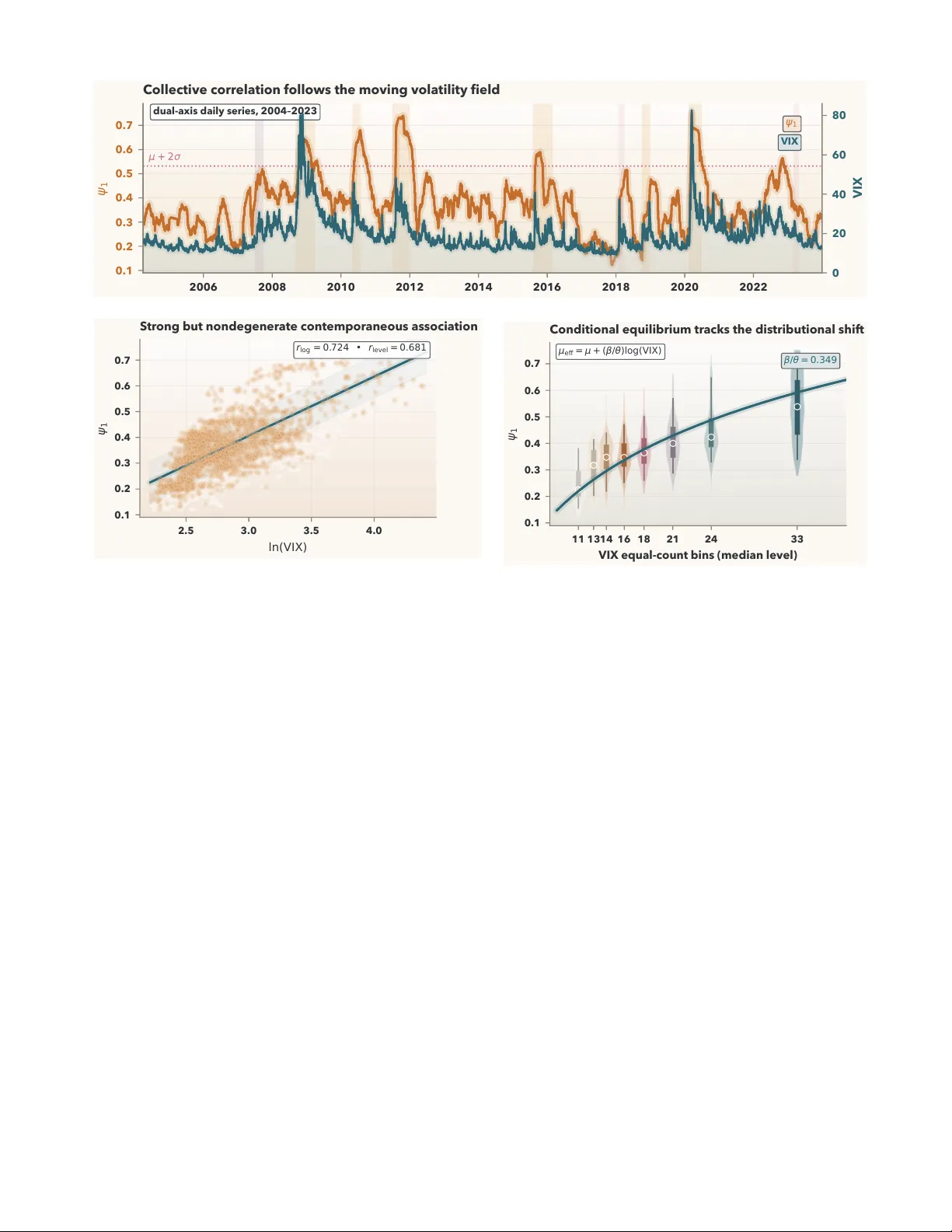
Conditioning on a V olatilit y Pro xy Compresses the Apparen t Timescale of Collectiv e Mark et Correlation Y uda Bi 1 , ∗ and Vince D. Calhoun 1, 2 1 Center for T r anslational R ese ar ch in Neur oimaging and Data Scienc e (TR eNDS), A tlanta, Ge or gia 30303, USA 2 Ge or gia State University, Ge or gia Institute of T e chnolo gy, and Emory University, Atlanta, Ge or gia 30303, USA (Dated: Marc h 17, 2026) W e address the attribution problem for apparent slow collective dynamics: is the observ ed p ersistence intrinsic, or inherited from a p ersisten t driv er? F or the leading eigenv alue fraction ψ 1 = λ max / N of S&P 500 60-da y rolling correlation matrices (237 sto c ks, 2004–2023), a VIX- coupled Ornstein–Uhlenbeck model reduces the eﬀectiv e relaxation time from 298 to 61 trading da ys and impro v es the ﬁt o ver bare mean reversion b y ∆BIC= 109. On the decomp osition sample, an informational residual of log(VIX) alone retains most of that gain (∆BIC= 78 . 6), whereas a mec hanical VIX proxy alone do es not impro ve the ﬁt. Auto correlation-matc hed placeb o ﬁelds fail (∆BIC max = 2 . 7), disjoint weekly reconstructions still fa vor the ﬁeld-coupled model (∆BIC= 140– 151), and six anc hored chronological holdouts preserv e the out-of-sample adv an tage. Quiet-regime and ﬁeld-stripp ed residual auto correlation con trols show the same collapse of p ersistence. Stronger hidden-v ariable extensions remain only partially supported. Within the tested stochastic class, conditioning on the observed VIX proxy absorbs most of the apparent slow dynamics. I. INTR ODUCTION A. Slo w collective observ ables pose an attribution problem Slo w collective observ ables are routinely interpreted as evidence for in trinsic memory , metastability , or critical slo wing do wn in complex systems [ 1 – 3 ]. The same em- pirical app earance can, how ever, arise when a mo der- ately relaxing observ able tracks an equilibrium that is itself displaced b y a persistent external or laten t ﬁeld [ 4 – 7 ]. Distinguishing these tw o mechanisms is diﬃcult whenev er the ﬁeld cannot b e turned on and oﬀ exper- imen tally , which is precisely the situation in ecological sync hrony , dynamic brain connectivity , and climate v ari- abilit y [ 1 , 2 , 7 ]. The ﬁrst logical task is therefore attri- bution: b efore p ositing intrinsic memory , one should ask whether the apparent persistence is inherited from the motion of a driver [ 4 , 6 , 8 ]. That attribution problem is sharper than a generic mo del-selection exercise [ 9 , 10 ]. A slow observ able can often b e ﬁt acceptably by several low-dimensional de- scriptions, including bare mean reversion, m ultistabil- it y , hidden-v ariable models, and explicit ﬁeld-coupled dy- namics [ 1 , 5 , 6 ]. Go od in-sample ﬁt alone therefore do es not establish mechanism [ 9 ]. What is needed is a se- quence of discriminations that asks whic h parts of the observ ed p ersistence survive conditioning, placeb o sub- stitution, and mo del-free con trols [ 4 , 7 , 8 ]. The present man uscript is built around that sequence. ∗ ybi3@gsu.edu B. Financial correlation dynamics pro vide a stringen t test case Financial mark ets oﬀer an unusually demanding testb ed b ecause they provide long, high-dimensional, and economically interpretable correlation time series [ 11 – 16 ]. Daily correlation matrices of large-cap U.S. equities exhibit a dominant market mo de that is stable enough to track ov er decades and strong enough to matter for systemic-risk interpretation [ 11 , 13 , 17 , 18 ]. A t the same time, the candidate ﬁeld pro xy is not cleanly exogenous: v olatility indices, realized co-mov emen t, and broad risk sen timent are partly entangled b y construction [ 19 – 22 ]. If an attribution w orkﬂo w works here, it is likely to trans- fer to cleaner domains rather than only to easier ones. The target of inference is therefore conditional attri- bution with resp ect to an observed ﬁeld proxy , not pro of of direct exogenous forcing [ 4 , 9 ]. That distinction mat- ters in ﬁnance b ecause the strongest plausible confound is a latent common driver that mo ves b oth VIX and the collectiv e correlation observ able [ 19 , 21 ]. The present de- sign is built to separate intrinsic persistence, p ersistence- only surrogates, and purely mec hanical o v erlap from that broader class of ﬁeld-pro xy explanations, while remain- ing explicit ab out what direct-coupling claims it cannot settle [ 8 , 9 ]. The ﬁnancial literature also supplies sharply com- p eting narrativ es [ 23 – 27 ]. One strand emphasizes en- dogenous collective reorganization, cascade ampliﬁca- tion, and near-critical dynamics [ 23 – 25 , 28 , 29 ]. Another strand emphasizes crisis-p eriod heteroskedasticit y , iden- tiﬁable macro-ﬁnancial sho c ks, and volatilit y-driven co- mo vemen t [ 17 , 19 – 22 ]. These views need not b e m utu- ally exclusiv e, but they imply diﬀerent exp ectations for the shap e of the eﬀective dynamics: in trinsic criticality p oin ts tow ard p ersisten t double-well or memory-bearing structure, whereas ﬁeld conditioning p oin ts tow ard a 2 comparativ ely simple observ able that relaxes around a mo ving equilibrium [ 1 , 5 , 6 ]. That distinction is exactly what the presen t tests are designed to prob e. Within that setting we study the leading-eigenv alue fraction ψ 1 ( t ) = λ max ( t ) tr C ( t ) = λ max ( t ) N , (1) where C ( t ) is the rolling P earson correlation matrix of sto c k returns. This quantit y inherits the main in tuition of random-matrix studies of ﬁnancial correlation, namely that the dominant eigenmo de captures collectiv e mark et- wide alignment while the bulk largely reﬂects noise and sectoral substructure [ 11 – 14 , 30 ]. It is also closely re- lated to the absorption ratio and to state-classiﬁcation approac hes based on the correlation spectrum [ 18 , 31 – 33 ]. What changes here is not the sp ectral ob ject, but the question: rather than using the leading mode as a static diagnostic, we treat it as a dynamical v ariable whose p ersistence itself must b e explained [ 34 – 37 ]. This c hoice is useful precisely b ecause ψ 1 remains collectiv e enough to track systemic episo des while remaining sim- ple enough to admit explicit sto c hastic comp etition be- t ween ﬁeld-free, ﬁeld-coupled, and hidden-v ariable mod- els [ 5 , 6 , 9 , 17 , 18 , 31 ]. C. The literature gap is not whether memory exists, but what causes it The immediate empirical bac kground is the generalized-Langevin work of W and, Heßler, and Kamps on the mean mark et correlation of the S&P 500 [ 38 , 39 ]. Their results are imp ortan t b ecause they show that a one-dimensional memory-bearing description of collectiv e mark et correlation is empirically viable and that the inferred memory kernel is not negligible [ 38 , 40 ]. More broadly , they connect ﬁnancial correlation dynamics to a gro wing literature on pro jected memory k ernels and hidden slo w v ariables in complex systems [ 4 , 7 , 41 , 42 ]. But that approach leav es op en a central causal question: do es the apparent memory remain once explicit external ﬁelds are introduced and compared against p ersistence-matc hed placeb o drivers [ 4 , 8 ]? That gap matters b ecause sev eral adjacen t literatures already suggest that volatilit y conditions strongly mo d- ulate correlations during crises [ 19 – 22 ]. The options- implied v olatility index VIX is esp ecially relev ant be- cause it is p ersisten t, forward-looking, and economically tied to broad uncertaint y sho c ks [ 20 , 21 , 43 ]. At the same time, VIX is partly mec hanical b ecause b oth VIX and realized correlation resp ond to the same underly- ing return cov ariance matrix [ 19 , 21 ]. A serious argu- men t for ﬁeld-driv en dynamics must therefore do more than report a high correlation b et ween VIX and ψ 1 . It must separate informational from mec hanical ov er- lap, show that p ersistence-matc hed surrogates fail, and test whether stronger hidden-v ariable interpretations still add an ything after the one-dimensional ﬁeld problem has b een settled [ 8 , 9 , 38 ]. Ev en then, a p ositiv e result against VIX should b e read as evidence that an observed ﬁeld pro xy carries struc- tured coupling information, not as pro of that the pro xy is the uniquely causal driver [ 4 , 9 , 19 ]. That is the infer- en tial level at which the pap er’s main claim is framed. D. This pap er provides a lay ered attribution test The man uscript pro ceeds in three deliberately unequal la yers. The ﬁrst lay er is the main result: w e compare ex- plicit one-dimensional sto c hastic mo dels and show that conditioning on an observ ed VIX ﬁeld pro xy absorbs most of the apparent p ersistence in ψ 1 within the tested sto c hastic class, while auto correlation-matc hed placeb o ﬁelds fail by a wide margin. The second lay er asks a harder question suggested b y the generalized-Langevin literature: can the observ ed VIX itself serve as the hidden co ordinate of an exact tw o-dimensional linear-Gaussian system whose pro jection generates memory [ 4 , 7 , 38 , 40 ]? The third lay er tests whether an orthogonal residual b e- y ond VIX functions as a meaningful secondary order pa- rameter or merely as a descriptiv e leftov er [ 9 , 44 ]. The evidential proﬁle is inten tionally asymmetric. The one-dimensional ﬁeld-pro xy attribution is strongly supp orted b y formal mo del comparison, placebo rejec- tion, directionality diagnostics, ﬁeld decomp osition, and mo del-free p ersistence collapse. The t wo-dimensional bridge survives only partially: it b ecomes more plausible under a W and-faithful weekly construction, but it do es not recov er the rep orted memory scale cleanly . The or- thogonal residual is descriptively nontrivial, but its fore- casting role is not supp orted. This asymmetry is a fea- ture rather than a ﬂa w, b ecause it k eeps the strongest claim tied to the strongest evidence [ 9 , 10 ]. The broader metho dological p oin t is transferable b e- y ond ﬁnance. An y system that supplies a collective ob- serv able and a candidate ﬁeld can be sub jected to the same logic: build the collective v ariable, compare bare and ﬁeld-coupled sto c hastic mo dels, reject p ersistence- only surrogates in the spirit of surrogate-data test- ing, and only then mo ve to stronger hidden-v ariable or residual-state interpretations [ 2 , 7 , 8 , 45 ]. The rest of the pap er follows that order. Section I I details the data, exp erimen tal design, and estimation procedures used throughout. Section I II presen ts the one-dimensional at- tribution result and its robustness tests, then the tw o- dimensional extension, and ﬁnally the orthogonal resid- ual analysis. Section IV discusses what these results do and do not imply for collective market dynamics and for the broader study of apparent slow mo des [ 1 , 4 , 38 ]. 3 I I. METHODS A. Data, alignmen t, and construction of the collectiv e observ able The daily baseline uses 237 S&P 500 constituents with con tinuous adjusted-close cov erage from 2004 through 2023. Daily log returns are computed in the usual wa y , r i ( t ) = log P i ( t ) − log P i ( t − 1), and 60-trading-da y rolling P earson correlation matrices are formed from those re- turns, following the standard correlation-matrix con- struction used throughout the ﬁnancial random-matrix literature [ 11 – 14 ]. The collective observ able is the leading-eigen v alue fraction ψ 1 ( t ) = λ max ( t ) tr C ( t ) = λ max ( t ) N , (2) where tr C = N b ecause C is a P earson correlation ma- trix with unit diagonal [ 11 , 13 , 15 ]. This observ able is the dynamic analogue of the dominan t market mo de empha- sized in random-matrix and absorption-ratio studies, but here it is treated as the dep enden t v ariable of a stochas- tic mo del rather than as a descriptive summary statistic [ 18 , 31 – 33 ]. Daily VIX closing v alues are aligned to the same trad- ing calendar using F ederal Reserve Economic Data. Af- ter alignment, the one-dimensional SDE sample contains n = 4973 daily observ ations from 2004-03-30 through 2023-12-29. On that aligned sample, ψ 1 has mean 0 . 3778, standard deviation 0 . 1171, and maximum 0 . 7518 dur- ing the C O VID-19 episo de. These levels are not in- terpreted as thermo dynamic in v arian ts; they dep end in part on the ﬁnite rolling-windo w estimator and on the high-dimensional asp ect ratio of the correlation matrices [ 14 , 15 , 30 ]. The ratio W/ N = 60 / 237 ≈ 0 . 25 places each rolling correlation matrix in a regime where the Marchenk o– P astur bulk edge is nontrivial [ 14 , 30 ]. That fact mat- ters for level interpretation b ecause the baseline v alue of ψ 1 con tains a stationary noise-ﬂo or contribution from ﬁnite-sample eigenv alue spreading [ 14 , 15 ]. It matters less for the present attribution exercise b ecause the pa- p er fo cuses on temp oral comparisons—auto correlation structure, mo del discrimination, and ﬁeld conditi oning— rather than on reading the absolute level of ψ 1 as a free-energy-lik e order parameter [ 9 , 15 , 16 ]. The same construction is recomputed directly from raw returns for W = 30 , 45 , 60 , 90 , 120 in the window-robustness experi- men t rep orted b elo w and in App endix C . B. Exp erimen tal design and eviden tial logic The em pirical design is sequen tial rather than om- nibus. Each stage is tied to a distinct riv al explana- tion for the observed slowness of ψ 1 [ 4 , 8 , 9 ]. The pri- mary comparison is b et ween a bare OU mo del, which attributes persistence to the observ able itself, and a VIX- coupled OU mo del, which attributes part of that persis- tence to motion of a ﬁeld-dep enden t equilibrium [ 5 , 6 , 21 ]. Quartic and regime-switching alternativ es are then added to test whether the data fav or endogenous multistabilit y or rare discrete stress states ov er the contin uous-ﬁeld pic- ture [ 23 , 46 , 47 ]. The main causal threat is that any suﬃcien tly p ersis- ten t driver might lo ok go od once inserted into the likeli- ho od. W e therefore deﬁne a formal placeb o gate in whic h the real VIX ﬁeld m ust b eat 100 p ersistence-matc hed surrogate ﬁelds generated from the ﬁtted marginal dy- namics of log (VIX) [ 8 ]. A second threat is circularity: VIX and ψ 1 are b oth functions of the same return co- v ariance matrix. T o address that concern w e decomp ose VIX into mechanical and informational comp onen ts, ﬁt eac h comp onen t as a standalone ﬁeld, and compare their mo del-selection p o wer directly [ 9 , 19 , 21 ]. The design then mov es outside the likelihoo d. Quiet- regime and ﬁeld-stripp ed autocorrelation tests ask whether p ersistence still collapses when the ﬁeld is ap- pro ximately dorman t or when the ﬁtted conditional equilibrium is remov ed. The exact window-size sw eep asks whether the ﬁeld eﬀect surviv es c hanges in time resolution. Disjoint weekly reconstructions and same- horizon disjoint 60-day blo c ks ask whether the core one- dimensional attribution surviv es once measuremen t o v er- lap is reduced or remov ed. Anchored chronological hold- outs ask whether the main result is tied to one histor- ical partition. MO VE and TED controls ask whether the ﬁeld picture is broader than VIX, while the ex- act t wo-dimensional mo del asks whether the observed VIX can itself close the hidden-v ariable bridge sug- gested by generalized-Langevin work [ 7 , 38 , 40 ]. Finally , the orthogonal residual analysis tests whether a VIX- orthogonal state v ariable carries op erational information b ey ond the main ﬁeld story [ 44 ]. This la yered design is delib erate. The pap er’s strongest claim is attac hed to the largest evidential stac k, not to the most ambitious theoretical extension [ 9 , 10 ]. The robustness pro cedures are sp eciﬁed here and written out in execution detail in Appendix B so that the paper reads as a tigh tly link ed sequence of discrimination tests rather than as a collection of disconnected chec ks. The design also has a clear inference b oundary . It can strongly distinguish bare in trinsic p ersistence from condi- tioning on an observed ﬁeld proxy , and it can separately test auto correlation-only and mechanical-o v erlap ob jec- tions. It cannot, b y itself, distinguish direct coupling from a latent common driv er that mov es b oth the pro xy and the observ able [ 4 , 9 , 19 ]. C. One-dimensional sto c hastic hierarch y and exact daily lik eliho od The core mo del comparison is inten tionally narro w. W e test whether the daily dynamics of ψ 1 are better 4 T ABLE I. Lay ered attribution logic. The strongest claim is the one that survives the largest stack of discrimination tests. Riv al explanation Primary discrimination Outcome in this man uscript Bare intrinsic p ersistence or auto correlation-only inheritance M0 versus M2, placeb o surrogates, quiet-regime ACF collapse, ﬁeld-stripp ed residual ACF, disjoint w eekly reconstructions, and anchored holdouts Strongly disfav ored Purely mechanical ov erlap b et w een VIX and ψ 1 Mec hanical/informational decomp osition, standalone ﬁeld tests, and recip e sensitivit y across freeze and weigh ting c hoices Strongly disfav ored dynamically Observ ed VIX as the exact hidden co ordinate b ehind pro jected memory Exact tw o-dimensional linear-Gaussian comparison and pro jected-kernel timescale chec k Only partially supp orted VIX-orthogonal residual as an op erational predictor Q2-v ersus-Q3 future-VIX test across 30-, 60-, and 90-day horizons Not supp orted describ ed b y bare mean reversion, by mean reversion around a ﬁeld-dep enden t equilibrium, or b y simple non- linear alternatives often asso ciated with metastability or eﬀectiv e double w ells [ 1 , 5 , 6 ]. The tw o central mo dels are dψ 1 = − θ 0 ( ψ 1 − µ 0 ) dt + σ 0 dW t , (3) dψ 1 = [ − θ ( ψ 1 − µ ) + β v t ] dt + σ dW t , (4) with v t = log(VIX t ). The ﬁrst mo del, M0, attributes all p ersistence to the observ able itself. The second mo del, M2, allo ws the equilibrium to slide with the volatilit y ﬁeld, so that µ eﬀ ( v ) = µ + ( β /θ ) v [ 5 , 6 , 21 ]. W e also ﬁt quartic-drift v arian ts with and without the ﬁeld, plus constrained tw o-state regime-switching comp etitors used only to calibrate whether a rare extreme-state c hannel adds structure beyond the contin uous ﬁeld [ 23 , 46 , 47 ]. F or M0 and M2, the exact one-step Gaussian transi- tion la w is av ailable in closed form b ecause the drift is linear conditional on the ﬁeld path. T reating v t as piece- wise constant ov er each daily interv al, the exact daily transition is ψ 1 ,t +1 | ψ 1 ,t , v t ∼ N ( m t , q ) , (5) with m t = e − θ ψ 1 ,t +  1 − e − θ   µ + β θ v t  , (6) q = σ 2 2 θ  1 − e − 2 θ  , (7) and the obvious M0 sp ecialization β = 0 [ 5 , 6 ]. The exact deriv ation is giv en in App endix A . W e maximize the resulting Gaussian likelihoo d directly for M0 and M2. Quartic v ariants are optimized n umerically under the same daily increment conv ention, and the constrained regime-switc hing mo dels are estimated with a Gaussian Hamilton ﬁlter under a tw o-state Marko v transition ma- trix [ 46 , 47 ]. Mo del comparison is based on BIC, with AIC recorded as a secondary diagnostic. Because all ﬁtted mo dels are coarse-grained approximations to a far richer mar- k et pro cess, the preferred sp eciﬁcation is interpreted in the pseudo-true sense of missp eciﬁed lik eliho od theory rather than as a literal data-generating law [ 9 ]. This p oin t matters for the timescale language used later: the rep orted τ auto = 1 /θ 0 and τ cond = 1 /θ are mo del-implied eﬀectiv e relaxation rates within the ﬁtted OU class, not claims ab out a unique microscopic law [ 6 , 9 ]. W e also test a heterosk edastic v arian t M2 ′ , deﬁned by the same OU+ﬁeld drift as M2 but with σ ( ψ 1 ) = σ 0 + σ 1 ψ 1 . (8) Because the diﬀusion co eﬃcien t is then state dep enden t, M2 ′ is ﬁt by direct numerical lik eliho od optimization un- der the same daily increment conv ention. Its role is di- agnostic rather than headline: it asks whether mo dest state-dep enden t noise c hanges the ﬁeld-attribution pic- ture [ 6 , 9 ]. Throughout the pap er we summarize the mo del-based ﬁeld con tribution by SCP A = 1 − τ cond τ auto = 1 − θ 0 θ , (9) whic h compares the conditioned and bare OU timescales directly . W e use the usual Jeﬀreys-st yle BIC scale only as an evidence summary , not as a substitute for robustness analysis [ 10 ]. The full execution details for the model- comparison pip eline are given in App endix B . D. Placeb o gate and the formal attribution null The strongest falsiﬁcation device is a placeb o-ﬁeld gate mo deled on surrogate-data logic [ 8 ]. W e ﬁt an AR( p ) model to v t = log (VIX t ), select p by AIC ov er p = 1 , . . . , 10, and obtain p = 9 on the aligned sample. W e then sim ulate 100 indep enden t surrogate ﬁelds from that ﬁtted marginal proc ess and rescale eac h surrogate to the empirical mean and v ariance of the real series. Eac h surrogate then replaces the real VIX ﬁeld in the same M2 likelihoo d. The formal null hypothesis is that the real VIX improv emen t can be matc hed by an indepen- den t realization drawn from the ﬁtted AR marginal la w of log(VIX). Under that n ull, any large BIC gain would b e attributable to generic p ersistence alone rather than 5 to sp eciﬁc coupling information [ 8 , 9 ]. Rejection there- fore means more than “VIX is p ersisten t”: it means that the observed driver carries coupling structure b ey ond its o wn auto correlation proﬁle. This placebo design is delib erately conserv ative. It do es not test against white noise or against an unrelated macro co v ariate, b oth of which would b e easy nulls. In- stead it tests against ﬁelds with essentially the same lo w- order temp oral persistence as the real series, which is the relev an t adv ersarial explanation for any claim ab out in- herited p ersistence [ 4 , 8 ]. The empirical p -v alue is the fraction of placebo gains that equal or exceed the real ∆BIC impro vemen t. Because only 100 placebos are used, the resolution is coarse, but the observed gap is so large that this discreteness is immaterial for the pap er’s con- clusions. The full placeb o proto col is written out in Ap- p endix B 1 . E. Directional diagnostics and mec hanical versus informational o verlap Directionalit y is ev aluated with man ual biv ariate Granger systems in b oth levels and ﬁrst diﬀerences. The lev el test chec ks whether lagged VIX terms improv e pre- diction of ψ 1 and vice versa. The diﬀerenced test is rep orted because near-integration can distort standard causalit y inference when p ersisten t series are used in lev- els [ 48 ]. These Granger results are not treated as the pri- mary identiﬁcation device b ecause rolling-window o ver- lap and mild missp eciﬁcation can still aﬀect them, but they provide a useful directional sanity chec k alongside the placeb o gate [ 9 , 48 ]. Mec hanical o verlap is estimated b y constructing a VIX pro xy that preserves the empirical correlation path while suppressing time v ariation in p er-stock volatilities. Con- cretely , for eac h sto c k i we compute its 60-day rolling v olatility series, take the median of that series o v er the aligned sample, replace the time-v arying v olatilit y b y that sto c k-speciﬁc median, and recompute an equal- w eight p ortfolio v ariance using the actual rolling corre- lation matrices. The square ro ot of that p ortfolio v ari- ance, after a single multiplicativ e rescaling to match the unconditional VIX level, deﬁnes the mechanical volatil- it y proxy . This construction is not intended to reproduce the full option-in tegral deﬁnition of VIX; it is a controlled decomp osition designed to ask how m uch of the ψ 1 as- so ciation survives after the common realized-cov ariance c hannel is stripp ed down to its correlation comp onen t [ 19 – 21 ]. The informational comp onen t is then deﬁned as the regression residual of actual log(VIX) on the mechanical pro xy . The mechanical and informational fractions re- p orted in the Results section come from a sequential R 2 decomp osition: ﬁrst regress ψ 1 on the mechanical proxy alone, then add the informational residual and record the incremen tal gain. The same tw o components are also inserted separately in to the M2 lik eliho od, producing standalone ﬁeld tests that directly assess whether mo del- selection p o wer lives in the mechanical channel, the in- formational c hannel, or b oth. The static v ariance split is op erational rather than unique, so we also rep eat the construction under alternativ e volatilit y-freezing choices and p ortfolio w eights. The point of those v ariants is not to force one canonical mec hanical/informational percent- age, but to test whether the sign and magnitude of the standalone ﬁeld gains are recip e dep enden t [ 9 , 19 ]. The exact algebra used for this decomposition is written out in App endix A , and the full execution proto col is given in App endix B 2 . F. Mo del-free p ersistence controls, non-ov erlapping reconstructions, and out-of-sample ev aluation The main one-dimensional claim is in tentionally c heck ed with con trols that do not depend on the OU lik eliho od. The ﬁrst is a quiet-regime autocorrelation comparison. Our strict ex ante criterion is daily VIX conﬁned to [15 , 18] for at least 120 consecutiv e trading da ys. Because that criterion yields no qualifying segmen t in 2004–2023, w e adopt a transparen t fallbac k based on a 20-da y rolling-median VIX in [14 , 20] and then r ep eat the calculation on neighboring bands [13 , 21] and [15 , 19]. F or eac h accepted set of quiet segments, the auto correlation function of ψ 1 is po oled across segmen ts and summarized b y the e-folding lag, deﬁned as the ﬁrst lag at which the A CF falls b elo w e − 1 of its lag-zero v alue. This diagnos- tic asks whether p ersistence collapses when the ﬁeld is appro ximately quiescent, without assuming any sp eciﬁc sto c hastic mo del. The second mo del-free control is the ﬁeld-stripped residual ϵ M2 ( t ) = ψ 1 ( t ) − µ eﬀ ( v t ) , (10) where µ eﬀ ( v t ) = µ + ( β /θ ) v t is the ﬁtted conditional equilibrium of M2. The ACF of ϵ M2 is compared with the ACF of raw ψ 1 through b oth e-folding lags and in- tegrated A CF mass ov er ﬁxed horizons. This control diﬀers conceptually from the OU timescale ratio. The timescale ratio asks how fast the mo del relaxes condi- tional on the ﬁeld; the residual ACF asks how m uch temp oral structure remains after subtracting the ﬁtted equilibrium path. The distinction is imp ortan t enough that the comparison is revisited explicitly in the Discus- sion section. F ull execution details for these controls are giv en in App endix B 3 . A deep er measurement concern is ov erlapping win- do ws. W e therefore rebuild the one-dimensional compar- ison on disjoin t weekly observ ables using 5-trading-day correlation windows sampled every 5 trading days, once for a weekly ψ 1 pro xy and once for w eekly mean mar- k et correlation. T o prob e the same-horizon extreme, we also construct disjoint 60-da y block versions of ψ 1 and pair each block with either its end-of-blo c k VIX v alue or its within-blo c k mean VIX [ 38 , 40 ]. These series are 6 lo wer pow er than the daily baseline, but they directly test whether the ﬁeld-coupled model remains preferred once ov erlap is reduced or remov ed at the observ able- construction stage. Their full execution details are also giv en in App endix B 4 . Out-of-sample stabilit y is assessed at tw o levels. The baseline split remains 2016-01-01: parameters are esti- mated on the pre-2016 observ ations and ev aluated on the p ost-2016 observ ations under the same exact one- step Gaussian likelihoo d. Beyond that baseline, we run an anchored split sweep at 2010-01-01, 2012-01-01, 2014- 01-01, 2016-01-01, 2018-01-01, and 2020-01-01, each time reﬁtting on the a v ailable preﬁx and ev aluating on the full remaining suﬃx. Performance is summarized by av erage log likelihoo d p er observ ation, the test/train ratio, and the test-set likelihoo d gap b et w een M2 and M0. This re- mains a chronological rather than cross-v alidated design, but it preven ts the stability claim from hinging on a sin- gle historical p artition [ 9 ]. The chronological holdout and anc hored-sweep proto cols are giv en in Appendix B 4 . G. Windo w-size robustness and resolution dep endence The windo w-robustness exp erimen t is designed to an- sw er a sp eciﬁc attac k: whether the baseline conditioned timescale near 61 trading days is merely a restatement of the 60-da y correlation windo w. W e therefore recompute ψ 1 directly from raw returns for W = 30 , 45 , 60 , 90 , 120, reﬁt M0 and M2 at eac h window, and record four quan ti- ties for every W : the bare timescale τ 0 = 1 /θ 0 , the condi- tioned timescale τ cond = 1 /θ , the susceptibilit y β /θ , and the scalar persistence-collapse attribution SCP A( W ) = 1 − τ cond ( W ) τ 0 ( W ) . (11) The point of this sweep is not to demand that abso- lute timescales b e iden tical across resolutions. Rolling correlation estimation is itself a lo w-pass ﬁlter, so abso- lute timescales can change mechanically with W . The relev an t structural question is instead whether the ﬁeld eﬀect—as summarized by the susceptibilit y and by the sign and magnitude of SCP A—survives across resolu- tions. The quantitativ e results of that sw eep are reported in App endix T able IV , and the full execution proto col is giv en in App endix B 4 . H. Exact t wo-dimensional extension and W and-faithful w eekly reconstruction T o test whether the observ ed VIX can itself pla y the role of the hidden v ariable b ehind apparent one- dimensional memory , we ﬁt the exact linear-Gaussian system dψ 1 = [ − θ ψ ( ψ 1 − µ ψ ) + β ψ v ] dt + σ ψ dW 1 , (12) dv = [ − θ v ( v − µ v ) + β v ψ 1 ] dt + σ v dW 2 , (13) with v = log(VIX) and correlated innov ations. In dis- crete time this is an exact V AR(1) transition mo del whose restriction pattern determines whether the drift is de- coupled, feedforward, or bidirectional [ 4 , 6 ]. The ﬁtted discrete transition matrix is mapped back to con tinuous time by matrix logarithm, and the innov ation cov ari- ance is matc hed through the discrete Ly apunov equa- tion, yielding exact contin uous-time parameters within the linear-Gaussian class. The pro jected-memory deriv a- tion asso ciated with this system is given in App endix A . The daily comparison alone is not enough b ecause o verlapping 60-day rolling windows c an accentuate se- rial dep endence. T o compare more fairly with W and et al. , w e therefore reconstruct disjoint weekly observ ables using 5-trading-day correlation windo ws sampled ev ery 5 trading days [ 38 , 40 ]. This reconstruction is p erformed t wice: once for a weekly ψ 1 pro xy computed from each disjoin t weekly matrix, and once for the mean mark et correlation of the same matrices. Both w eekly series are passed through the same exact tw o-dimensional model comparison and pro jected-kernel calculations. This de- sign keeps the hidden-v ariable test close to the prepro- cessing assumptions of the generalized-Langevin litera- ture while preserving direct comparability with the daily mo del family . F ull execution details for the 2D compari- son are giv en in Appendix B 5 . I. Orthogonal residual state v ariable The ﬁnal construction is a level-orthogonal residual b e- y ond the ﬁtted conditional equilibrium. W e estimate ϵ ⊥ ( t ) = ψ 1 ( t ) − [ a + b log (VIX( t ))] , (14) using ordinary least squares on lev els, so that ϵ ⊥ is ap- pro ximately uncorrelated with log(VIX) b y construction. This ob ject is not the same as ϵ M2 . The latter strips the ﬁtted M2 equilibrium and is useful for p ersistence attribution; the former strips only the b est linear lev el relation and is useful for asking whether an additional VIX-orthogonal state v ariable carries descriptive or pre- dictiv e structure. W e then partition the (log VIX , ϵ ⊥ ) plane by the sample median of log VIX and by the sign of ϵ ⊥ , pro ducing the four quadrants used in the ﬁnal re- sults section. The prop osed predictive test compares future VIX c hanges after Q2 days (low VIX, p ositiv e ϵ ⊥ ) against Q3 da ys (low VIX, negative ϵ ⊥ ). W e rep ort mean future c hanges, Mann–Whitney p -v alues, and rank-biserial ef- fect sizes at 30-, 60-, and 90-trading-day horizons. This is inten tionally a narrow op erational claim. A residual can b e dynamically non trivial without qualifying as a forecasting signal, and the analysis is designed to keep those tw o prop ositions separate [ 9 , 44 ]. 7 I II. RESUL TS A. Empirical target The quantit y to explain is not merely the existence of crisis episo des with elev ated collective correlation, but the fact that the full-sample auto correlation of ψ 1 re- mains elev ated for months. Figure 1 sho ws that ψ 1 co- mo ves strongly with VIX across the 2004–2023 sample while still exhibiting appreciable residual scatter around the observed volatilit y ﬁeld proxy . The question through- out is whether this slow-looking b eha vior is intrinsic to ψ 1 or inherited from the motion of that observ ed proxy . B. Conditional ﬁeld-pro xy decomp osition The one-dimensional sto c hastic hierarch y yields the clearest result of the paper. T able II summarizes the main mo del comparison. The main reference mo del re- mains the VIX-coupled Ornstein–Uhlenbeck mo del [ 5 , 6 , 21 ], dψ 1 = [ − θ ( ψ 1 − µ ) + β log(VIX)] dt + σ dW, (15) with b est-ﬁt parameters θ = 0 . 01640, µ = − 0 . 6256, β = 0 . 00572, and σ = 0 . 00942. The asso ciated eﬀectiv e equilibrium is µ eﬀ (VIX) = µ + β θ log(VIX) , (16) whic h ev aluates numerically to µ eﬀ (VIX) = − 0 . 626 + 0 . 349 log(VIX) on the aligned sample. This linear ap- pro ximation is intended only o ver the observed VIX range of roughly 10–80. Extrap olation far b elo w that range w ould imply unphysical negative equilibria once VIX falls b elo w about 6, which simply reﬂects the lo cal nature of the linearization. A t the baseline 60-day correlation-window construc- tion, tw o timescales separate sharply . In the bare OU mo del, θ 0 = 0 . 00335, giving an apparent relaxation time of roughly 298 trading days. In the VIX-coupled OU mo del, the intrinsic relaxation time conditional on the observ ed VIX proxy is roughly 61 trading days. The ratio 298 / 61 ≈ 4 . 9 means that, in OU-rate terms, conditioning on the observed VIX proxy remo ves ab out 79 . 5% of the apparen t p ersistence. These timescales should b e under- sto od as mo del-implied relaxation rates under the ﬁtted linear OU appro ximation, consistent with the pseudo- true interpretation adopted throughout. The global BIC winner is the h ybrid constrained regime-switc hing plus VIX mo del. Its ﬁtted parameters, ho wev er, make its role quite sp eciﬁc: the calm state car- ries 98 . 7% of the stationary probability , the stress state lasts only ab out 1 . 1 trading days on av erage, and the con tinuous VIX loading remains large ( β = 0 . 00781). In other w ords, the hybrid mo del is b est read as a rare T ABLE II. Core one-dimensional and h ybrid stochastic mo d- els on the aligned daily sample. Mo del BIC ∆BIC vs M2 M RS,c+VIX -33011.9 -765.4 M RS,c -32274.4 -27.9 M2’ -32255.3 -8.7 M2 -32246.5 0.0 M3 -32230.0 +16.5 M0 -32137.5 +109.0 M1 -32121.5 +125.0 extreme-ev ent channel lay ered on top of the same con- tin uous ﬁeld eﬀect isolated by M2 [ 46 , 47 ]. The nested lik eliho od-ratio test against the regime-switching base- line is also decisive ( χ 2 = 746, p ≈ 0), so the hybrid ﬁt v alidates the co existence of discrete extremes and con tin- uous ﬁeld motion rather than replacing the M2 interpre- tation [ 9 , 46 ]. Within the hybrid mo del, the calm-state parameters imply an intrinsic timescale of roughly 43 trading da ys. The corresp onding timescale ratio is there- fore 1 − 43 / 298 ≈ 0 . 86, slightly ab o v e the M2-based es- timate of 0 . 80. The qualitative conclusion is unchanged: most apparen t p ersistence is ﬁeld-inherited under either the M2 lens or the BIC-winning hybrid mo del. Com- plete parameter estimates for M RS,c+VIX are rep orted in App endix T able X . Tw o negative results are equally central. A quartic mo del without an explicit ﬁeld is strongly disfav ored rel- ativ e to the VIX-coupled OU mo del, and adding quar- tic structure on top of VIX do es not improv e the ﬁt. Within the tested mo del family , the collective dynamics do not support a double-well or Ising-lik e in terpretation [ 23 , 28 , 29 ]. The state-dependent-noise v arian t M2 ′ pro vides only a mo dest reﬁnement. Allowing σ ( ψ 1 ) = σ 0 + σ 1 ψ 1 im- pro ves BIC by 8 . 7 units relative to M2, indicating some structured heteroskedasticit y , but it do es not impro v e the most diﬃcult high-VIX PIT diagnostic. W e therefore re- tain the constant- σ M2 model as the primary interpretiv e lens and read M2 ′ as a secondary adequacy chec k rather than as a change in the central attribution story [ 6 , 9 ]. C. Placeb o falsiﬁcation and robustness controls The strongest single discrimination test is the placebo- ﬁeld exp erimen t [ 8 ]. W e generate 100 AR(9)-matched syn thetic ﬁelds that repro duce the ﬁrst-order p ersistence structure of log (VIX) and compare their impro v ements against the real VIX ﬁeld. None of the 100 surrogates matc hes the real VIX gain. The resulting distribution has mean ∆BIC= − 6 . 5, standard deviation 2 . 19, and maxim um 2 . 70, versus 109 . 0 for the real VIX ﬁeld. This excludes an explanation based on autocorrelation matc h- ing alone [ 8 , 9 ]. Directionalit y supp orts the same picture. In the level- 8 2006 2008 2010 2012 2014 2016 2018 2020 2022 0.1 0.2 0.3 0.4 0.5 0.6 0.7 ψ 1 Collective corr elation follows the moving volatility field dual-axis daily series, 2004–2023 ψ 1 VIX 0 20 40 60 80 VIX 2.5 3.0 3.5 4.0 l n ( V I X ) 0.1 0.2 0.3 0.4 0.5 0.6 0.7 ψ 1 Str ong but nondegener ate contempor aneous association r l o g = 0 . 7 2 4 • r l e v e l = 0 . 6 8 1 11 13 14 16 18 21 24 33 VIX equal-count bins (median level) 0.1 0.2 0.3 0.4 0.5 0.6 0.7 ψ 1 Conditional equilibrium tr acks the distributional shif t μ e f f = μ + ( β / θ ) l o g ( V I X ) β / θ = 0 . 3 4 9 (a) (b) (c) FIG. 1. Collective correlation trac ks a mo ving volatilit y ﬁeld. (a) The long-run ψ 1 series co-mov es strongly with VIX o ver 2004–2023, with the largest excursions concentrated in ma jor crisis episodes. (b) The contemporaneous asso ciation is strong but nondegenerate, with r = 0 . 724 against log(VIX) and r = 0 . 681 against level VIX. (c) Equal-count VIX bins show that the ﬁtted conditional equilibrium µ eﬀ (VIX) = µ + ( β /θ ) log(VIX) tracks the empirical shift of the ψ 1 distribution across v olatility conditions. T ogether these panels motiv ate the attribution problem addressed b elo w. based Granger system, VIX → ψ 1 dominates with F = 15 . 07 at lag 7, while the reverse direction is not signiﬁcant in lev els. Under ﬁrst diﬀerencing, VIX still dominates ( F = 10 . 63 versus 2 . 76), so the directional asymmetry is not a simple rolling-window ov erlap artifact [ 48 ]. The endogeneity ob jection is nevertheless real [ 19 , 21 ]. Using the actual rolling correlation structure together with ﬁxed median sto c k volatilities, we estimate that roughly 77 . 3% of the shared explanatory p o wer in the VIX– ψ 1 relationship is mec hanical and 22 . 7% is informa- tional, with a partial residual correlation of ab out 0 . 60. Th us VIX is not a clean exogenous proxy in the strict ph ysical sense. But the informational incremen t is sub- stan tial, and the placebo failure shows that it is not re- placeable by generic p ersistence. The strongest new evidence comes from ﬁtting these t wo comp onen ts as standalone ﬁelds. On the restricted sample where the split is deﬁned, an M2 ﬁt using the in- formational residual of log(VIX) alone still improv es on the bare OU benchmark b y ∆BIC= 78 . 6, whereas the mec hanical proxy alone do es not improv e on the b enc h- mark at all (∆BIC= − 8 . 3). The full VIX ﬁeld on that same restricted sample yields ∆BIC= 108 . 6 (App endix T able V ). In other words, the part of VIX that carries mo del-selection p o w er is ov erwhelmingly informational rather than mechanical. The comp onen t gains are not exp ected to add up exactly , since the OU parameters are re-estimated for each eﬀective ﬁeld, but the dynamic implication is unambiguous: the main ﬁeld-proxy attri- bution is not b eing generated b y trivial ov erlap b et w een realized volatilit y and realized correlation [ 9 , 19 ]. That dynamic conclusion is not tied to a single decom- p osition recip e. Across three volatilit y-freezing c hoices (full-sample median, full-sample mean, and pre-2016 median) and three weigh ting schemes (equal, inv erse- v olatility , and v olatility-share), the static mec hanical fraction mov es from 72 . 1% to 81 . 5% while the infor- mational fraction mo ves from 18 . 5% to 27 . 9% (Ap- p endix T able VI ). But the dynamic result is in v ari- an t: informational-only ﬁelds remain strongly p ositiv e with ∆BIC in the narrow range 77 . 7–79 . 6, whereas mec hanical-only ﬁelds remain BIC-negative in every tested v arian t ( − 8 . 38 ≤ ∆BIC ≤ − 8 . 27). The static split is therefore op erational rather than unique, while the dynamic conclusion is highly stable across reasonable constructions [ 9 , 19 ]. 9 −50 0 50 100 Δ B I C r e l a t i v e t o M 2 M_RS,c+VIX M_RS,c M2' (state-dep. σ) M2 (OU+VIX) M6 (VIX+MOVE) M3 (quartic+VIX) M_RS (unconstr ained) M4 (MOVE) M5 (TED) M0 (bar e OU) M1 (quartic) -765.4 -27.9 -8.7 mechanistic lens +8.5 +16.5 +36.5 +96.9 +103.4 +109.0 +125.0 Model hier ar chy ar ound the field-coupled OU lens bet ter than M2 worse than M2 C o n d i t i o n e d τ c o n d A p p a r e n t τ a u t o 0 50 100 150 200 250 300 Relaxation time (tr ading days) 61 d 298 d Conditioning on VIX collapses the headline timescale 4.9× slower without field conditioning b a s e l i n e W = 6 0 0 20 40 60 80 100 Δ B I C u n d e r p l a c e b o s u b s t i t u t i o n 0 5 10 15 20 25 30 Count Real VIX ΔBIC = 109 placebo max = 2.7 P ersistence-matched placebo fields fail by a huge mar gin placebo mean = -6.5 max placebo = 2.7 • r eal = 109.0 Dir ectionality points fr om the volatility field to the collective variable VIX ψ 1 F = 1 5 . 1 , p < 1 0 − 1 5 F = 1 . 6 , p = 0 . 1 4 5 (a) (b) (c) (d) FIG. 2. The main attribution result. (a) Same-sample model comparison across the core, hybrid, and auxiliary-ﬁeld v arian ts centers the main in terpretive story on the VIX-coupled OU mo del: bare OU and quartic alternatives are strongly disfa vored, while rare-ev ent h ybrids are better read as an added extreme-state channel than as a replacemen t for the contin uous ﬁeld picture. (b) Under the baseline W = 60 construction, conditioning on VIX reduces the relaxation time from 298 to 61 trading days. (c) One hundred AR-matched placeb o ﬁelds fail to approach the real-VIX gain (maximum placeb o ∆BIC = 2 . 7 versus 109 for real VIX). (d) Lev el-based Granger tests show dominant VIX → ψ 1 directionalit y ( F = 15 . 1 versus 1 . 6 in the rev erse direction). These panels together establish the conditional ﬁeld-proxy attribution that anchors the rest of the man uscript. The ov erlapping-window concern can also b e brough t directly to the core one-dimensional claim. Rebuild- ing the observ able from disjoin t 5-trading-da y correlation matrices sampled every 5 trading days, the ﬁeld-coupled OU still b eats bare mean reversion by ∆BIC= 151 . 2 for w eekly ψ 1 and b y ∆BIC= 140 . 1 for w eekly mean mark et correlation (App endix T able VI I ). On those dis- join t weekly series the eﬀective timescales shorten, as ex- p ected from the coarser clo c k, but the sign of the attri- bution result is unc hanged: SCP A remains p ositiv e at 0 . 286 and 0 . 282, resp ectiv ely . At the opp osite extreme, a same-horizon disjoin t 60-da y blo c k reconstruction yields only ∆BIC= 1 . 7 when paired with end-of-blo c k VIX and ∆BIC= − 3 . 4 when paired with blo c k-mean VIX. W e therefore interpret that 60-day blo c k v ersion as a low- p o w er b oundary chec k with only 77 observ ations, not as a p o w er-matc hed replacement for the daily series. The main point is narrow er but decisiv e: once o verlap is re- mo ved in a reasonably information-preserving weekly re- construction, the ﬁeld-coupled mo del remains strongly preferred [ 9 , 38 , 40 ]. Cross-mark et auxiliary ﬁelds are weak er. MOVE pro- vides only a mo dest same-sample gain (∆BIC= 12 . 0 ver- sus the bare mo del), while TED do es not impro ve the ﬁt (∆BIC= − 1 . 1). Several reasonable transformations of MO VE yield the same conclusion: it is auxiliary , not de- cisiv e. The strongest cross-ﬁeld statement the curren t ev- idence supp orts is therefore mo dest: VIX is the uniquely strong ﬁeld proxy in this dataset, MOVE is secondary , and TED does not help. The stochastic ﬁts are complemen ted b y t wo mo del- free con trols. The ﬁrst is a quiet-regime autocorrelation c heck. The physically motiv ated strict criterion—daily VIX inside [15 , 18] for at least 120 consecutiv e trading da ys—yields no qualifying segment in the entire sam- ple. That absence is itself informative: the v olatility ﬁeld is never truly dorman t for long, consistent with contin- ual mo dulation of ψ 1 [ 1 , 21 ]. T o obtain a ﬁnite-sample 10 quiet-regime estimate, w e therefore adopt a transparent relaxed criterion based on a 20-day rolling-median VIX in [14 , 20], which yields three qualifying segmen ts. Under that deﬁnition the e-folding lag drops from 69 days to 27 da ys, with an episo de-bo otstrap 95% conﬁdence in terv al of [18 , 33] days, the A CF at lag 20 falls from 0 . 853 to 0 . 514, and by lag 40 the quiet-regime ACF has already crossed below zero. The same 27-day e-folding lag is re- co vered under the wider [13 , 21] band, whereas the nar- ro wer [15 , 19] band yields no qualifying 120-day segment at all (App endix T able IX ). The quiet-regime diagnos- tic is therefore partially robust: it is replicated across the tw o widest tested bands, but ﬁnite-sample supp ort disapp ears at the narrow est band. The second control is a ﬁeld-stripp ed residual. Deﬁn- ing ϵ M2 ( t ) = ψ 1 ( t ) − µ eﬀ (VIX( t )) , (17) w e ﬁnd that the residual remains p ersisten t, but muc h less so than raw ψ 1 : the e-folding lag drops from 69 to 42 da ys, the integrated ACF up to lag 60 drops from 44 . 3 to 30 . 6, and the integrated ACF up to lag 90 drops from 54 . 2 to 38 . 7. Field stripping therefore does not annihilate all persistence, but it remov es a substan tial fraction of it. These controls are supp orted by a broader out-of- sample chec k. The baseline split at 2016-01-01 leav es the p er-observ ation log likelihoo d of M2 almost unchanged b et w een train and test p eriods (3 . 252 versus 3 . 235, ra- tio 0 . 995), which argues against the main result b eing a crisis-sp eciﬁc in-sample artifact. Because the p ost-2016 holdout con tains the CO VID-19 spike, w e also repeat the ev aluation after excluding 2020-03-01 through 2020-09- 30 and scoring the tw o remaining contiguous test seg- men ts separately . The test log likelihoo d per observ a- tion then rises to 3 . 310, with a test/train ratio of 1 . 018, so the stability claim do es not dep end on the COVID episo de. More imp ortan tly , a six-wa y anc hored split sw eep at 2010, 2012, 2014, 2016, 2018, and 2020 leav es the sign of the result unc hanged on every held-out re- mainder: M2 b eats M0 on test in all six cases, with per- observ ation test-set gains ranging from 0 . 0023 to 0 . 0152 and M2 test/train ratios ranging from 0 . 964 to 0 . 999 (Ap- p endix T able VI II ). The ﬁeld-coupled adv antage is there- fore not tied to a single historical partition [ 9 ]. An exact ra w-return window sweep sharp ens the in ter- pretation of the headline timescale. Recomputing ψ 1 di- rectly from returns for W = 30 , 45 , 60 , 90 , 120 leav es the ﬁeld adv an tage intact at ev ery window (∆BIC= 99–165 for M2 ov er M0) and k eeps the ﬁeld susceptibility β /θ in a narrow range of 0 . 336–0 . 376 (Appendix T able IV ). The absolute conditioned timescale is not window-in v arian t: it rises from 34 trading days at W = 30 to 97 trading da ys at W = 120, while the bare timescale rises from 105 to 839 days. This b eha vior is exp ected from the low-pass ﬁltering inherent in rolling-windo w estimation. The more structural quan tit y is the susceptibility β /θ , which deter- mines the equilibrium displacement p er unit of log(VIX) and remains stable across all tested windo ws. The at- tribution fraction itself, measured by 1 − τ cond /τ auto , re- mains ma jority-inherited at every window but increases from 0 . 67 to 0 . 88 rather than staying strictly constan t. The 61-da y ﬁgure should therefore be read as the ef- fectiv e conditioned timescale at the baseline resolution W = 60, not as a window-independent physical constant [ 6 , 9 ]. The monotonic increase of SCP A with W is itself consisten t with rolling-window low-pass ﬁltering, which inﬂates the bare timescale more strongly b ecause the bare mo del must absorb ﬁeld-driv en slow motion that the conditioned mo del remov es explicitly . The formal limit W → 0 is not an operational ob ject for rolling-correlation estimation: while the leading eigen v alue fraction remains estimable in the high-dimensional W < N regime, arbi- trarily short windows w ould collapse the statistic in to ﬁnite-sample noise [ 14 ]. The smallest analyzed window here is W = 30, where the bare timescale is still 105 trad- ing days, already well ab o ve the window length itself. D. Tw o-dimensional hidden-v ariable extension The strongest theoretical extension w as to ask whether the observ ed VIX can itself serve as the hidden v ari- able b ehind one-dimensional generalized Langevin mem- ory [ 4 , 38 , 40 ]. The following extension is exact only within the linear-Gaussian class, with nonlinear depar- tures treated as a limitation rather than silently absorb ed in to the interpretation [ 6 , 9 ]. T o test this, we ﬁt an exact linear-Gaussian tw o-dimensional system, dψ 1 = [ − θ ψ ( ψ 1 − µ ψ ) + β ψ v ] dt + σ ψ dW 1 , (18) dv = [ − θ v ( v − µ v ) + β v ψ 1 ] dt + σ v dW 2 , (19) with v = log(VIX) and correlated innov ations. Because the one-step transition densit y is exactly Gaussian, the discrete V AR(1) lik elihoo d is the exact transition-densit y MLE within this mo del family . On the aligned daily series, feedforward coupling is preferred o ver bidirectional drift by ∆BIC= 2 . 4, while the feedforward mo del b eats the decoupled mo del by ∆BIC= 125 . 3. The ∆BIC= 2 . 4 margin b et ween feed- forw ard and bidirectional drift is small by conv en tional mo del-selection standards [ 10 ], so the daily data of- fer only a weak preference for the simpler feedforward form. The preferred daily mo del repro duces the one- dimensional M2 parameters on the ψ 1 side almost ex- actly , but sets β v = 0 in the b est structure. On the daily sample, observed VIX b eha v es as a p ersisten t driver, not as a preferred hidden v ariable whose elimination gener- ates a self-memory kernel [ 4 , 38 ]. The key stress test is therefore the W and-faithful w eekly construction. The daily series is built from ov er- lapping windows, which can accentuate serial dep endence and ma y sharp en the app earance of one-w ay drive. W e therefore rebuild the problem using disjoint 5-day cor- relation windows sampled ev ery 5 trading days, m uc h closer to the preprocessing in the generalized-Langevin 11 0 10 20 30 40 50 60 70 80 90 Lag (tr ading days) 0.0 0.2 0.4 0.6 0.8 1.0 A CF full sample field-stripped quiet r egime P ersistence collapses under quiet-field r estriction and field stripping quiet = 27 d r esidual = 42 d full = 69 d 0 20 40 60 80 100 Δ B I C v s M 0 VIX VIX+MOVE MOVE TED 109.0 100.4 12.0 -1.1 VIX r emains uniquely str ong among candidate driving fields same-sample comparisons 0 20 40 60 80 100 Δ B I C v s M 0 o n d e c o m p o s i t i o n s a m p l e Actual VIX Informational Mechanical 108.6 78.6 -8.3 Standalone field tests Mechanical Informational Mechanical vs informational split 77.3% 22.7% p a r t i a l r = 0 . 6 0 0 20 40 60 80 100 120 R o l l i n g w i n d o w W ( d a y s ) 1 10 100 1000 Timescale (days) τ a u t o τ c o n d Resolution-dependent timescales b a s e l i n e W = 6 0 0 20 40 60 80 100 120 R o l l i n g w i n d o w W ( d a y s ) 0.3 0.4 0.5 0.6 0.7 0.8 0.9 Dimensionless r esponse 0.336 0.337 0.349 0.370 0.376 β / θ 1 − τ c o n d / τ a u t o Stable susceptibility , varying at tribution (a) (b) (c) (d) FIG. 3. Indep enden t robustness chec ks. (a) Persistence collapses b oth in quiet regimes and after subtracting the ﬁtted VIX-dep enden t equilibrium: the full-sample e-folding lag is 69 trading days, the ﬁeld-stripped residual falls to 42 days, and the quiet-regime estimate falls to 27 days. (b) Among auxiliary ﬁelds, VIX remains uniquely strong, while MO VE is secondary and TED do es not improv e on the bare b enc hmark. (c) On the decomposition sample, the informational residual of log(VIX) alone retains most of the model-selection gain (∆BIC = 78 . 6), whereas the mechanical proxy alone fails to improv e the ﬁt (∆BIC = − 8 . 3); the same sample still yields a 77 . 3% / 22 . 7% mec hanical/informational v ariance split. (d) Exact recomputation across W = 30–120 shows that absolute timescales dep end on rolling-windo w resolution, but the ﬁeld susceptibilit y β /θ stays in the narro w range 0 . 336–0 . 376 and the attribution fraction remains ma jority-inherited at ev ery window. T ogether these panels show that the main claim is not an artifact of placebo p ersistence, auxiliary ﬁelds, mechanical o verlap, or the baseline window c hoice. literature [ 38 , 40 ]. Under this construction the evidence c hanges: a w eekly ψ 1 pro xy weakly prefers the full bidi- rectional model by ∆BIC= 0 . 78 ov er feedforward, and the weekly mean market correlation w eakly prefers it by ∆BIC= 2 . 69. This is the strongest surviving part of the hidden- v ariable story: bidirectional structure b ecomes more plausible once the comparison is made under a prepro- cessing regime close to the prior weekly w ork. But the bridge still stops short of full iden tiﬁcation [ 4 , 7 ]. Solv- ing the second equation formally and substituting into 12 the ﬁrst yields a pro jected memory term of the form K ( t ) = β ψ β v e − θ v t , (20) plus colored-noise contributions. The implied timescales are not close to the conserv ativ e ∼ 15-day b enc hmark implied by “three trading weeks” in W and et al. On our outputs they are approximately 36 . 5 days for the daily full mo del, 9 . 1 days for naiv e weekly thinning, 33 . 5 days for the W and-faithful w eekly ψ 1 pro xy , and 36 . 5 days for the W and-faithful mean mark et correlation. The bridge is therefore nontrivial but incomplete: a more faithful w eekly comparison makes bidirectional coupling more plausible, y et observed VIX still do es not recov er the re- p orted generalized-Langevin memory scale. The 2D placeb o gate still adds independent v alue. The daily feedforw ard mo del beats the daily decoupled model b y roughly 125 BIC units, and none of 100 AR-matched placeb o ﬁelds repro duces the real coupling gain. So the 2D section remains essential even though it supports only partial reconciliation rather than full uniﬁcation. E. Orthogonal residual analysis The ﬁnal analytical step asks whether a residual order parameter b ey ond VIX can carry op erational informa- tion. Tw o residuals are useful to distinguish [ 9 , 44 ]. The mec hanistic residual, ϵ M2 ( t ) = ψ 1 ( t ) − µ eﬀ (VIX( t )) , (21) is natural for ﬁeld-stripping but not orthogonal to VIX in lev els. The relev an t candidate order parameter is instead the orthogonal lev el residual, ϵ ⊥ ( t ) = ψ 1 ( t ) − ( a + b log (VIX( t ))) , (22) where ( a, b ) are estimated from a direct lev el regression and therefore enforce corr( ϵ ⊥ , log VIX) ≈ 0. This v ariable is not trivial noise. Its e-folding lag is ab out 43 days, compared with 69 days for raw ψ 1 , and its integrated ACF to lag 60 is 32 . 1 instead of 44 . 3. In that sense, ϵ ⊥ is a genuine residual mode rather than a negligible leftov er. The asso ciated phase-space program is only partially successful. P artitioning the (log VIX , ϵ ⊥ ) plane by the sample median of log VIX and the sign of ϵ ⊥ yields bal- anced time fractions o v erall, but ev en t-p eak classiﬁcation is less ric h than hop ed: Q1 contains six p eak even ts, Q4 con tains three, Q2 contains only China/Oil 2015–16, and Q3 contains none of the predeﬁned ev en t p eaks. Thus the phase space is descriptive, but not a mature four-state taxonom y . The strongest prop osed operational test also fails. Comparing lo w-VIX/high- ϵ ⊥ (Q2) da ys against low- VIX/lo w- ϵ ⊥ (Q3) days, we ﬁnd no evidence that Q2 pre- cedes larger future VIX increases at 30, 60, or 90 trad- ing days. The mean diﬀerences are small, the Mann– Whitney tests are not signiﬁcan t, and the asso ciated T ABLE I I I. F uture VIX changes after low-VIX da ys split by the sign of the orthogonal residual. Positiv e rank-biserial v al- ues would fav or the prop osed Q2 signal. Horizon Mean Q2 Mean Q3 Mann–Whitney p Rank-biserial 30 days 0.078 0.083 0.183 0.021 60 days 0.082 0.135 0.736 -0.015 90 days 0.110 0.141 0.986 -0.052 rank-biserial eﬀect sizes remain close to zero (T able I II ). The orthogonal residual therefore survives as a descrip- tiv e state v ariable, but not as a demonstrated forecasting signal. T ak en together, the results deﬁne a delib erately unev en evidence proﬁle: the conditional ﬁeld-proxy decomp osi- tion is strongly supp orted, the tw o-dimensional bridge is only partially supp orted, and the orthogonal residual is descriptiv e rather than predictive. IV. DISCUSSION The central result is conditional rather than fully causal: within the tested sto c hastic class, most appar- en t p ersistence in market collective correlation is ab- sorb ed once one conditions on an observed VIX ﬁeld pro xy rather than leaving the dynamics bare. The strongest con tribution of the pap er is therefore not a univ ersal hidden-v ariable model, but a falsiﬁable attri- bution protocol that sharply narrows the interpretation of slow collectiv e dynamics [ 4 , 8 , 9 ]. A ﬁeld-coupled OU mo del, a placeb o gate that rejects auto correlation- matc hed surrogates, disjoint weekly reconstructions that preserv e the M2 adv antage, decomp osition v arian ts that lea ve informational-only ﬁelds strongly p ositiv e while mec hanical-only ﬁelds remain negative, and b oth quiet- regime and ﬁeld-stripp ed ACF collapse all p oin t in the same direction. This conv ergence is unusually strong for a soft-system inference problem [ 19 , 20 , 43 , 49 ]. A. Reconciling p ersistence attribution measures Tw o quan titative attribution measures app ear in this pap er and should not b e conﬂated. The timescale ratio 1 − τ cond /τ auto ≈ 0 . 80 compares mo del-implied OU relax- ation rates b efore and after conditioning on VIX [ 5 , 6 ]. By contrast, the ﬁeld-stripped residual ACF reduction of ab out 39% compares the e-folding lag of raw ψ 1 against that of ϵ M2 = ψ 1 − µ eﬀ (VIX), dropping from 69 to 42 trading days. The ﬁrst quantit y is a mo del-based rate comparison within the OU class; the second is a mo del- free comparison of the temp oral structure left after sub- tracting the ﬁtted conditional equilibrium. These num bers need not agree. The timescale ratio measures ho w fast ψ 1 relaxes to ward a moving VIX- dep enden t target once that target is speciﬁed. The resid- 13 −3 −2 −1 0 1 2 3 B I C f u l l − B I C f e e d f o r w a r d Daily aligned W e e k l y ψ 1 W eekly mean corr . +2.44 -0.78 -2.69 Bidir ectional mar gin negative favors bidir ectional positive favors feedforwar d Daily full W eekly-thin W e e k l y ψ 1 W eekly mean corr . 0 5 10 15 20 25 30 35 40 K ernel timescale (days) 36.5 9.1 33.5 36.5 P r ojected-k ernel timescales W and benchmark ≈ 15 d 2.5 3.0 3.5 4.0 4.5 l o g ( V I X ) −0.2 −0.1 0.0 0.1 0.2 0.3 ε ⟂ Orthogonal r esidual state space is structur ed but still descriptive GFC '08 Eur o '11 China '15 COVID '20 SVB '23 Q2 Q1 Q3 Q4 30d 60d 90d 0.000 0.025 0.050 0.075 0.100 0.125 0.150 0.175 M e a n f u t u r e Δ l o g ( V I X ) Q2 Q3 T he pr oposed Q2–Q3 for ecasting contr ast r emains null p = 0 . 1 8 3 p = 0 . 7 3 6 p = 0 . 9 8 6 (a) (b) (c) FIG. 4. Extensions b ey ond the main one-dimensional result. (a) On daily aligned data the 2D comparison weakly fa vors feedforward ov er bidirectional drift by ∆BIC = 2 . 44, whereas the W and-faithful weekly reconstructions weakly fav or bidirectionalit y (∆BIC = − 0 . 78 for weekly ψ 1 and − 2 . 69 for weekly mean correlation; negativ e v alues fav or bidirectional coupling). The pro jected-kernel timescales remain in the 9–36 da y range and therefore do not recov er the 15-da y W and b enc hmark in any clean w ay . (b) The orthogonal residual phase space in (log VIX , ϵ ⊥ ) is structured and visually nontrivial. (c) The prop osed Q2-v ersus-Q3 prediction test nevertheless remains null across all tested horizons ( p = 0 . 183, 0 . 736, and 0 . 986 at 30, 60, and 90 trading da ys). The ﬁgure therefore frames these sections as constrained extensions rather than as new headline results. ual ACF measures how muc h p ersistence remains af- ter that target is subtracted, including p ersistence from imp erfect linearization, additional latent drivers, and rolling-windo w measurement structure [ 6 , 9 ]. They there- fore brack et the ﬁeld eﬀect from diﬀeren t angles rather than estimating a single universal p ercen tage. A further cav eat is that the absolute OU timescales are resolution-dependent. Exact recomputation with W = 30–120 sho ws that the conditioned relaxation time increases from 34 to 97 trading da ys as the rolling window lengthens, which is consisten t with the low-pass ﬁltering built in to rolling-window observ ables [ 6 , 9 ]. The more structural quantit y is the susceptibilit y β /θ , which re- mains stable across those windows in the narrow range 0 . 336–0 . 376. By con trast, the mo del-based attribution fraction 1 − τ cond /τ auto is not strictly inv ariant: it stays in the ma jority-inherited regime for every window, but rises from ab out 0 . 67 to 0 . 88 as W increases. The baseline 61-da y estimate should therefore b e read as the eﬀective conditioned timescale of the standard W = 60 construc- tion, not as a window-free microscopic constant. The t wo-dimensional extension reﬁnes that conclusion without ov erturning it. On the aligned daily sample, ob- serv ed VIX b eha v es as a persistent driver and not as the preferred hidden co ordinate whose pro jection w ould repro duce generalized-Langevin memory . A t the same time, the W and-faithful weekly reconstruction do es re- viv e w eak bidirectional preference, though still within the inconclusive BIC range, so the relation to W and et al. is more n uanced than simple con tradiction. W e also note that the W and sample (1992–2012, N = 249) dif- fers from ours in b oth p eriod and sto c k univ erse, so part of the kernel-timescale discrepancy may reﬂect data dif- ferences rather than a fundamental failure of the Mori– Zw anzig identiﬁcation. The most defensible synthesis is partial reconciliation: explicit ﬁeld driving and hidden- 14 v ariable memory are not unrelated descriptions, but ob- serv ed VIX alone does not complete the Mori–Zwanzig iden tiﬁcation [ 4 , 7 , 38 , 40 ]. The orthogonal residual extension leads to a paral- lel lesson. Constructing ϵ ⊥ is easy , and its dynam- ics are not trivial. It yields a genuine VIX-orthogonal residual mo de with intermediate p ersistence and some ev ent-classiﬁcation structure. But that is not the same as demonstrating an operationally useful predictive or- der parameter [ 9 ]. The negative Q2-v ersus-Q3 tests sho w why it is worth keeping those claims separate. This residual also diﬀers conceptually from the implied- correlation v ersus realized-correlation gaps studied in the correlation-risk-premium literature [ 44 ]: here the ob- ject is an orthogonalized collective state v ariable, not an option-pricing spread. These results sharp en the relation to the criticality lit- erature. The presen t evidence does not supp ort a double- w ell, Ising-lik e, or critical-slo wing interpretation of ψ 1 dy- namics [ 1 , 23 – 27 ]. Within the tested sto c hastic class, the ph ysical picture is closer to a driv en single-well system with p ersistent ﬁeld motion and a mo dest complemen- tary extreme-state channel [ 5 , 6 ]. Strong visual p ersis- tence of the collective v ariable is therefore not, by itself, evidence for a near-critical endogenous transition [ 1 , 9 ]. This also clariﬁes the relation to earlier Kramers– Mo yal extractions for ﬁnancial correlation observ ables. Unlik e Stepanov et al. , who extracted Kramers–Moy al co eﬃcien ts for a related dominating correlation v ariable without testing external ﬁelds explicitly , the present w ork conditions on candidate drivers and sub jects them to placeb o-surrogate discrimination [ 8 , 42 ]. More broadly , the metho dology should transfer to other soft complex systems. Dynamic functional con- nectivit y in fMRI or EEG, dela yed climate indices, and ecological sync hron y measures all face the same question: is the slow observ able intrinsically slow, or is it b eing dragged b y a p ersisten t ﬁeld pro xy [ 1 , 2 , 7 ]? The same placeb o-con trolled sequence used here can b e applied there as w ell: compare bare and ﬁeld-coupled stochas- tic mo dels, reject p ersistence-only surrogates, quantify mec hanical o verlap where needed, and only then test stronger hidden-v ariable or residual-state interpretations [ 4 , 7 , 8 ]. Exact m ultiv ariate OU ﬁts also open a route to nonequilibrium diagnostics such as en tropy-production measures [ 45 ]. Abstracted aw ay from ﬁnance, the protocol has four generic ingredients: a collectiv e observ able, an observed candidate ﬁeld proxy on the same clo c k, a ﬁeld-free v er- sus ﬁeld-coupled sto c hastic comparison with matched lik eliho od treatment, and an adversarial surrogate or decomp osition stage that attac ks p ersistence-only and mec hanical-only explanations [ 4 , 8 , 9 ]. It is strongest when the observ able can be reconstructed at m ultiple res- olutions and when a non-ov erlapping v ersion is av ailable. Its generic failure mode is latent common driv e: if an un- observ ed z mov es b oth the pro xy and the observ able, the proto col can still sho w that conditioning on the pro xy re- mo ves apparent p ersistence, but it cannot by itself prov e direct coupling from proxy to observ able [ 4 , 7 , 9 ]. B. Limitations Sev eral limits remain important. First, the VIX rela- tionship is materially mechanical ev en after the decompo- sition [ 19 , 21 ]. The static mec hanical share is op erational rather than unique: across reasonable freeze and weigh t- ing schemes it ranges from 0 . 72 to 0 . 81, even though the dynamic mo del-selection conclusion remains inv ariant. Second, MO VE and TED do not supp ort a broader cross- mark et hierarch y b ey ond the main VIX result. Third, the t wo-dimensional extension is exact only within a linear- Gaussian class, and the state-dep enden t-noise diagnos- tics indicate structured inadequacies in extreme regimes [ 6 , 9 ]. F ourth, the even t sample is still small relative to the breadth of ﬁnancial stress phenomenology . Fi- nally , the main failure mo de of the attribution protocol is a latent common driver that is only imp erfectly prox- ied by the observed ﬁeld proxy; placeb o rejection against the observed proxy do es not eliminate that p ossibilit y [ 4 , 9 ]. More precisely , the placeb o gate tests whether the observed pro xy carries coupling information b ey ond marginal p ersistence, but it do es not by itself distinguish direct coupling u → y from a confounded structure in whic h an unobserved driver z inﬂuences b oth the proxy u and the observ able y . These cav eats deﬁne the paper’s b oundary rather than its weakness. The manuscript is strongest on conditional ﬁeld-pro xy attribution, more limited on the hidden- v ariable bridge, and explicitly negativ e on operational residual prediction. These boundaries delineate what can and cannot be concluded from the present evidence. D A T A A V AILABILITY Daily VIX closes w ere obtained from F ederal Reserve Economic Data. The pro cessed datasets needed to repro- duce the ﬁgures and tables in this manuscript are a v ail- able from the authors on reasonable request. CODE A V AILABILITY The analysis and ﬁgure-generation co de used for this man uscript are av ailable from the authors on reasonable request. 15 App endix A: Exact Likelihoo ds and Analytical Deriv ations 1. Exact one-dimensional transition la ws F or the bare OU mo del, dψ t = − θ 0 ( ψ t − µ 0 ) dt + σ 0 dW t , (A1) the exact solution ov er one unit daily interv al is ψ t +1 = e − θ 0 ψ t +  1 − e − θ 0  µ 0 + η t , (A2) with Gaussian inno v ation η t ∼ N (0 , q 0 ) , (A3) q 0 = σ 2 0 2 θ 0  1 − e − 2 θ 0  , (A4) whic h is the standard exact transition density of the Ornstein–Uhlenbeck pro cess [ 5 , 6 ]. The one-step log likelihoo d is ℓ M0 = − n − 1 2 log(2 π q 0 ) − 1 2 q 0 n − 1 X t =1  ψ t +1 − m (0) t  2 , (A5) where m (0) t = e − θ 0 ψ t + (1 − e − θ 0 ) µ 0 . F or the ﬁeld-coupled mo del, dψ t = [ − θ ( ψ t − µ ) + β v t ] dt + σ dW t , (A6) w e treat the observed ﬁeld v alue v t = log(VIX t ) as constan t on the interv al [ t, t + 1). V ariation of constan ts gives ψ t +1 = e − θ ψ t + Z t +1 t e − θ ( t +1 − s ) ( θ µ + β v t ) ds + Z t +1 t e − θ ( t +1 − s ) σ dW s . (A7) The deterministic in tegral ev aluates to  1 − e − θ   µ + β θ v t  , (A8) and the stochastic integral is Gaussian with v ariance σ 2 (1 − e − 2 θ ) / (2 θ ) [ 5 , 6 ]. Hence ψ t +1 | ψ t , v t ∼ N  m (2) t , q  , (A9) m (2) t = e − θ ψ t +  1 − e − θ   µ + β θ v t  , (A10) q = σ 2 2 θ  1 − e − 2 θ  . (A11) The corresp onding log likelihoo d is ℓ M2 = − n − 1 2 log(2 π q ) − 1 2 q n − 1 X t =1  ψ t +1 − m (2) t  2 . (A12) 16 The quantities rep orted in the main text are then τ auto = 1 θ 0 , (A13) τ cond = 1 θ , (A14) χ = β θ , (A15) µ eﬀ ( v ) = µ + χv, (A16) where χ is the ﬁeld susceptibilit y , i.e. the equilibrium displacement p er unit of log(VIX). 2. Mec hanical and informational ﬁeld decomp osition Let m t denote the mechanical volatilit y proxy and a t = log(VIX t ) denote the actual ﬁeld. The informational residual is deﬁned by the auxiliary regression a t = γ 0 + γ 1 m t + r t , (A17) so that r t is orthogonal to the ﬁtted mec hanical comp onen t in sample. W e then ﬁt the sequential regressions ψ t = α 0 + α 1 m t + u t , (A18) ψ t = β 0 + β 1 m t + β 2 r t + ε t . (A19) If R 2 mech is the co eﬃcien t of determination of the ﬁrst regression and R 2 full that of the second, the rep orted fractions are f mech = R 2 mech R 2 full , (A20) f info = R 2 full − R 2 mech R 2 full . (A21) With the decomp osition sample used in the manuscript, R 2 full = 0 . 7120, R 2 mech = 0 . 5505, and the informational incremen t is 0 . 1615, yielding f mech = 0 . 7732 and f info = 0 . 2268. These quantities summarize shared explanatory p o w er in a static regression sense; they do not imply that the s t andalone OU-ﬁeld impro vemen ts m ust add linearly , b ecause the M2 parameters are re-estimated for each ﬁeld and the ﬁtted equilibrium map c hanges with the ﬁeld deﬁnition [ 9 ]. That is precisely why the separate M2 ﬁts with actual, mechanical-only , and informational-only ﬁelds are rep orted as distinct exp erimen ts rather than algebraically com bined. 3. Tw o-dimensional OU pro jection and induced memory k ernel W rite the cen tered tw o-dimensional system as ˙ x ( t ) = A x ( t ) + Σ ξ ( t ) , (A22) x ( t ) =  ψ 1 ( t ) − µ ψ v ( t ) − µ v  , (A23) with drift matrix A =  − θ ψ β ψ β v − θ v  . (A24) The exact discrete transition ov er one in terv al ∆ is x t +∆ = e A ∆ x t + η t , (A25) η t ∼ N (0 , Q ∆ ) , (A26) 17 with cov ariance Q ∆ = Z ∆ 0 e As ΣΣ ⊤ e A ⊤ s ds, (A27) whic h is the exact contin uous-time/discrete-time corresp ondence for linear-Gaussian systems [ 4 , 6 ]. The structural restrictions used in the pap er are: decoupled ( β ψ = β v = 0), feedforward ( β ψ  = 0 , β v = 0), and bidirectional ( β ψ  = 0 , β v  = 0). The daily and weekly comparisons are carried out b y exact Gaussian likelihoo d in this discrete represen tation, and the contin uous-time coeﬃcients are obtained b y matrix logarithm of the estimated transition matrix. T o exp ose the pro jected-memory interpretation, solve the second equation formally: v ( t ) = v (0) e − θ v t + Z t 0 e − θ v ( t − s ) [ β v ψ 1 ( s ) ds + σ v dW 2 ( s )] . (A28) Substituting this expression into the observ able equation yields ˙ ψ 1 ( t ) = − θ ψ ψ 1 ( t ) + β ψ v (0) e − θ v t + β ψ β v Z t 0 e − θ v ( t − s ) ψ 1 ( s ) ds + β ψ σ v Z t 0 e − θ v ( t − s ) dW 2 ( s ) + σ ψ ξ 1 ( t ) . (A29) The induced self-memory kernel is therefore K ( t ) = β ψ β v e − θ v t , (A30) and the associated pro jected timescale is τ K = 1 /θ v [ 4 , 7 ]. When β v = 0, as in the daily-preferred feedforward structure, this kernel v anishes identically . The observ ed VIX can only generate a nonzero pro jected memory kernel when the bidirectional term is empirically supp orted. 4. Deﬁnitions of attribution measures Tw o attribution measures are used rep eatedly in the manuscript. The ﬁrst is the mo del-based scalar p ersistence- collapse attribution SCP A = 1 − τ cond τ auto = 1 − θ 0 θ , (A31) whic h compares OU timescales b efore and after ﬁeld conditioning. The second is the mo del-free ﬁeld-stripp ed p ersis- tence reduction, computed from the e-folding lag or in tegrated ACF of ψ 1 v ersus that of ϵ M2 = ψ 1 − µ eﬀ ( v ). These measures are not expected to coincide exactly because they summarize diﬀerent ob jects: one is a rate parameter inside the ﬁtted OU class, while the other is a residual temp oral statistic that remains sensitive to latent driv ers, nonlinearit y , and rolling-windo w measuremen t eﬀects [ 6 , 9 ]. The manuscript therefore interprets them jointly rather than forcing them into a single p ercen tage. App endix B: Robustness Exp erimen t Design and Execution 1. Placeb o-ﬁeld proto col The placeb o exp erimen t is executed as a ﬁxed pip eline rather than as an informal sensitivity chec k. First, we ﬁt an AR( p ) mo del to the aligned log(VIX) series, selecting p by AIC ov er p = 1 , . . . , 10; this chooses p = 9 on the aligned sample. Second, w e sim ulate 100 indep enden t surrogate paths of the same length as the empirical ﬁeld, using the ﬁtted AR recursion and indep enden t Gaussian inno v ations. Third, each path is linearly rescaled to the empirical mean and v ariance of the real log(VIX) series so that only the coupling information, not the marginal scale, can 18 diﬀeren tiate the real and placeb o ﬁelds. F ourth, eac h surrogate replaces the real ﬁeld in the exact M2 likelihoo d, and the impro vemen t ov er M0 is recorded as ∆BIC placebo . Fifth, the empirical p -v alue is computed as the fraction of placeb o gains that meet or exceed the real gain [ 8 , 9 ]. The same logic is reused in the 2D daily placeb o gate, where feedforw ard and full bidirectional models are compared against the decoupled b enc hmark under p ersistence-matc hed placeb o drivers. 2. Mec hanical-proxy construction and standalone ﬁeld tests The mec hanical pro xy is constructed on the same aligned daily sample used for the main M2 ﬁt. F or each sto c k i , let s i,t denote the 60-day rolling v olatility and let ˜ s i = median t s i,t b e its sample median ov er the aligned p eriod. With equal portfolio w eights w i = 1 / N , the mec hanical p ortfolio v ariance is b V mech t = N X i =1 N X j =1 w i w j ˜ s i ˜ s j C ij ( t ) . (B1) The mechanical VIX proxy is then VIX mech ,t = c q b V mech t , (B2) where the scalar c is chosen so that the proxy matches the sample mean of the observed VIX. The informational comp onen t is deﬁned by residualizing log(VIX t ) on log(VIX mech ,t ). The design then b ranches in to t wo complemen tary ev aluations. A static regression decomposition yields the mec hanical and informational fractions of shared explanatory p o w er. Separate M2 ﬁts using the actual ﬁeld, the mechanical proxy , and the informational residual then ask whic h comp onen t carries standalone mo del-selection p o wer. The key inference is dynamic rather than purely correlational: ev en if the mechanical proxy is highly correlated with ψ 1 , it do es not count as explanatory unless it improv es the sto c hastic lik eliho od o ver M0. T o test recip e sensitivit y , w e repeat the construction under three volatilit y-freezing statistics and three weigh ting sc hemes. The freeze v arian ts are the full-sample median, the full-sample mean, and the pre-2016 median of eac h sto c k’s 60-day rolling v olatility . The weigh ting v ariants are equal weigh ts, inv erse-v olatility weigh ts, and volatilit y- share weigh ts. Every v arian t is pushed through the same t wo outputs: the static regression decomp osition and the standalone M2 ﬁts with mechanical-only and informational-only ﬁelds. This k eeps the sensitivity analysis aligned to the reviewer’s actual concern, namely whether the qualitative mo del-selection conclusion c hanges under reasonable alternativ e constructions. 3. Quiet-regime p ooling and ﬁeld-stripp ed A CF ev aluation The quiet-regime exp erimen t is executed in tw o passes. The strict pass scans the aligned daily sample for maximal con tiguous segments in which the daily VIX level remains inside [15 , 18] for at least 120 consecutive trading days. When that yields no v alid segment, the fallback pass replaces the ra w daily VIX by a 20-da y rolling median and scans three neighboring bands: [13 , 21], [14 , 20], and [15 , 19]. F or each band, all maximal con tiguous segmen ts with length at least 120 trading days are retained. Within each segment we compute the sample ACF of ψ 1 , then p ool the segmen t-sp eciﬁc ACFs by av ailable pair counts at each lag. The e-folding lag is rep orted as the ﬁrst lag at which the p ooled ACF falls b elo w e − 1 . F or the baseline rolling-median band [14 , 20], ﬁnite-sample uncertaint y is quan tiﬁed b y resampling the qualifying quiet episo des with replacemen t, which preserves within-episo de serial dep endence, and recomputing the po oled e-folding lag ov er 5000 b ootstrap dra ws. The ﬁeld-stripp ed residual exp erimen t uses the ﬁtted M2 equilibrium path, ϵ M2 ( t ) = ψ 1 ( t ) − µ eﬀ ( v t ) , (B3) computed on the same aligned sample. W e compare the e-folding lag and the integrated A CF mass of ra w ψ 1 and ϵ M2 o ver ﬁxed horizons of 60 and 90 trading days. This pairing is inten tional: the quiet regime remov es ﬁeld v ariation b y sample restriction, whereas the residual exp eriment remov es the ﬁtted equilibrium path algebraically . Agreement b et w een the tw o strengthens the attribution claim b ecause it shows p ersistence collapse under tw o conceptually distinct manipulations. 19 4. Windo w sweep, non-ov erlapping reconstructions, auxiliary ﬁelds, and out-of-sample sw eeps The window sw eep is conducted by recomputing ψ 1 from raw daily returns at ﬁve windo w lengths: W = 30 , 45 , 60 , 90 , 120. No smo othing appro ximation is used; each series is reconstructed from the returns and then aligned to the daily VIX ﬁeld o ver the corresp onding date range. At each W , M0 and M2 are ﬁt from scratc h and four outputs are retained: τ 0 , τ cond , β /θ , and SCP A = 1 − τ cond /τ 0 . This proto col cleanly separates resolution dep endence from co de reuse, and it also provides an exact chec k that the W = 60 reconstruction repro duces the baseline order parameter. T o confron t o verlap directly , we also reconstruct disjoin t w eekly observ ables from 5-trading-da y correlation matrices sampled every 5 trading days. This is done t wice: once for a weekly ψ 1 pro xy and once for weekly mean market correlation, b oth aligned to weekly VIX closes [ 38 , 40 ]. F or a same-horizon b oundary c heck, we construct disjoin t 60-trading-da y blo c ks of ψ 1 and pair each blo c k with either its end-of-blo c k VIX level or its within-blo c k mean VIX. These lo w-frequency series are in tentionally retained ev en when underpow ered, because their role is to sho w ho w m uc h of the core attribution survives when measurement ov erlap is aggressively remov ed. Auxiliary-ﬁeld controls are run on the maximal same-sample intersections with the respective ﬁelds. MOVE is tested by ﬁtting an OU+MOVE mo del and then a t wo-ﬁeld OU+VIX+MOVE mo del on the in tersection sample. TED is tested by ﬁtting an OU+TED model on its own maximal in tersection sample. The same BIC logic is used in every case. This design a v oids misleading comparisons across unequal date ranges while still showing whether non-VIX ﬁelds carry indep enden t dynamic information. Out-of-sample ev aluation is run at tw o lev els. The baseline c hronological holdout uses a single split at 2016-01-01. P arameters are estimated on the pre-2016 sample and scored on the p ost-2016 sample with the same exact one-step Gaussian likelihoo d. W e rep ort the av erage log likelihoo d on train and test and their ratio. Because the test set includes the COVID-19 perio d, the holdout is meaningfully harder than a random split and therefore functions as a basic stability stress test for the conditional ﬁeld-proxy claim. As a sensitivit y c heck, we also exclude 2020-03-01 through 2020-09-30 from the test p eriod and score the pre- and post-COVID test segments separately , so that no one-step increment is ev aluated across the excluded gap. T o av oid hinging on one split, we then run an anchored sw eep with cut dates at 2010-01-01, 2012-01-01, 2014-01-01, 2016-01-01, 2018-01-01, and 2020-01-01. F or each split, M0 and M2 are ﬁt on the av ailable preﬁx and scored on the entire held-out suﬃx under the same exact one-step Gaussian likelihoo d. The rep orted outputs are the M2 and M0 test log lik eliho ods p er observ ation, the M2 − M0 test gap, and the M2 test/train ratio. This design does not con vert the problem into indep enden t folds, but it do es sho w whether the ﬁeld-coupled adv antage survives repeated c hronological re-estimation. 5. Tw o-dimensional hidden-v ariable proto col and residual-state test The 2D hidden-v ariable proto col is run ﬁrst on the daily aligned ( ψ 1 , log VIX) series and then on tw o W and-faithful w eekly reconstructions. In each dataset we ﬁt three exact linear-Gaussian mo dels: decoupled, feedforward, and bidirectional. The comparison is based on exact Gaussian likelihoo d and BIC. When the bidirectional mo del wins, we compute the pro jected kernel amplitude and timescale implied by the ﬁtted contin uous-time matrix. The stage gate is not whether any bidirectional mo del exists, but whether the observed VIX yields b oth bidirectional preference and a pro jected timescale compatible with the generalized-Langevin b enc hmark. That is wh y the daily , w eekly-thinning, and W and-faithful reconstructions are all retained. The residual-state test uses the orthogonalized lev el residual ϵ ⊥ rather than the mec hanistic residual ϵ M2 . After splitting the (log VIX , ϵ ⊥ ) plane into four quadrants, we p erform a fo cused forecasting comparison b et ween Q2 and Q3 b ecause that contrast captures the only genuinely op erational claim prop osed during manuscript dev elopment: conditional on low VIX, do es a p ositiv e orthogonal residual predict a larger future increase in VIX than a negativ e one? W e rep ort mean future c hanges, Mann–Whitney p -v alues, and rank-biserial eﬀect sizes at 30, 60, and 90 da ys. The design is inten tionally narrow so that the result is either a clean p ositiv e or a clean negative rather than a diﬀuse narrativ e ab out state-space geometry . 20 T ABLE IV. Exact window-size robustness of M0 and M2, recomputing ψ 1 directly from raw returns at eac h windo w. SCP A denotes 1 − τ cond /τ auto . W θ 0 τ 0 θ τ cond β β /θ SCP A ∆BIC 30 0.00955 104.67 0.02927 34.17 0.00982 0.336 0.674 104.0 45 0.00553 180.79 0.02093 47.78 0.00706 0.337 0.736 99.4 60 0.00335 298.10 0.01640 60.99 0.00572 0.349 0.795 109.0 90 0.00194 516.68 0.01317 75.93 0.00488 0.370 0.853 153.6 120 0.00119 838.72 0.01036 96.55 0.00390 0.376 0.885 165.4 T ABLE V. M2 ﬁts with actual, mechanical-only , and informational-only ﬁelds on the decomp osition sample. Field θ τ cond β ∆BIC vs M0 (decomp. sample) Actual log (VIX) 0.01723 58.05 0.00623 108.6 Mec hanical-only pro xy 0.00393 254.18 0.00026 -8.3 Informational residual 0.00850 117.67 0.00471 78.6 T ABLE VI. Sensitivity of the mechanical/informational decomposition to volatilit y-freezing and weigh ting choices. The static split is recip e dependent, but the standalone dynamic conclusion is inv ariant across all tested v arian ts. Recip e Mec hanical fraction Informational fraction ∆BIC mech-only ∆BIC info-only Median freeze, equal weigh ts 0.773 0.227 -8.35 78.59 Mean freeze, equal weigh ts 0.776 0.224 -8.36 78.73 Pre-2016 median freeze, equal weigh ts 0.779 0.221 -8.34 78.62 Median freeze, inv erse-v olatilit y w eights 0.815 0.185 -8.27 77.71 Median freeze, volatilit y-share weigh ts 0.721 0.279 -8.38 79.57 T ABLE VI I. One-dimensional non-ov erlapping robustness chec ks. The disjoint weekly reconstructions preserv e strong supp ort for M2, whereas same-horizon 60-day block reconstructions are retained only as low-pow er b oundary c hecks. Construction n obs ∆BIC M2 vs M0 τ 0 (trading days) τ cond (trading days) SCP A Daily ov erlapping baseline 4973 109.0 298.10 60.99 0.795 Disjoin t w eekly ψ 1 976 151.2 8.24 5.88 0.286 Disjoin t w eekly mean correlation 976 140.1 8.43 6.05 0.282 Disjoin t 60-da y blo c ks, end-of-blo c k VIX 77 1.7 89.48 64.69 0.277 Disjoin t 60-da y blo c ks, blo c k-mean VIX 77 -3.4 89.48 75.05 0.161 T ABLE VI II. Anchored c hronological out-of-sample sweep. F or each split date, M0 and M2 are ﬁt on the pre-split preﬁx and ev aluated on the full held-out suﬃx. Split date n train n test M0 test ll/obs M2 test ll/obs M2 − M0 test gap M2 test/train ratio 2010-01-01 1451 3522 3.1931 3.2000 0.0070 0.964 2012-01-01 1955 3018 3.2227 3.2373 0.0146 0.994 2014-01-01 2457 2516 3.2294 3.2437 0.0143 0.999 2016-01-01 2961 2012 3.2219 3.2346 0.0128 0.995 2018-01-01 3464 1509 3.1653 3.1805 0.0152 0.972 2020-01-01 3967 1006 3.2301 3.2324 0.0023 0.995 T ABLE IX. Quiet-regime band sensitivit y . The strict daily band [15 , 18] with a 120-trading-day minim um yields zero qualifying segmen ts ov er 2004–2023. F or the baseline rolling-median band [14 , 20], the quiet e-folding estimate of 27 da ys carries an episode- b ootstrap 95% conﬁdence interv al of [18 , 33] days. Rolling-median VIX band Segmen ts ≥ 120d Quiet e-folding lag F ull-sample e-folding lag [13 , 21] 5 27 69 [14 , 20] 3 27 69 [15 , 19] 0 — 69 21 T ABLE X. Parameters of the constrained regime-switching plus VIX mo del M RS,c+VIX on the aligned daily sample. P arameter or derived quantit y Estimate θ 0.02348 µ calm -0.6021 µ stress 1.0000 β 0.00781 σ 0.00818 p calm → stress 0.01170 p stress → calm 0.8940 Exp ected calm duration (days) 85.5 Exp ected stress duration (days) 1.12 Stationary calm probability 0.9871 Stationary stress probability 0.0129 Calm-state relaxation time (days) 42.6 T ABLE XI. Exact t wo-dimensional mo del comparisons and pro jected-kernel timescales across the daily and W and-faithful datasets. The rep orted ∆BIC v alues are relative to the winning mo del in each panel. Dataset Winning structure ∆BIC vs next-b est ∆BIC vs decoupled Kernel timescale (days) Daily aligned ψ 1 F eedforward 2.44 125.26 36.46 (full mo del only) Naiv e w eekly thinning F eedforward 4.17 74.45 9.10 (full mo del only) W and-faithful weekly ψ 1 Bidirectional 0.78 154.10 33.47 W and-faithful weekly mean correlation Bidirectional 2.69 143.87 36.46 App endix C: Supplementary Quantitativ e T ables [1] M. Scheﬀer, J. Bascompte, W. A. Bro c k, V. Brovkin, S. R. Carp en ter, V. Dakos, H. Held, E. H. v an Nes, M. Rietkerk, and G. Sugihara, Nature 461 , 53 (2009). [2] E. A. Allen, E. Damara ju, S. M. Plis, E. B. Erhardt, T. Eichele, and V. D. Calhoun, Cerebral Cortex 24 , 663 (2014). [3] R. F riedrich, J. Peink e, M. Sahimi, and M. Reza Rahimi T abar, Ph ysics Rep orts 506 , 87 (2011). [4] R. Zwanzig, None quilibrium Statistic al Me chanics (Oxford Universit y Press, 2001). [5] H. Risken, The F okker–Planck Equation: Metho ds of Solution and Applic ations (Springer, 1996). [6] C. W. Gardiner, Sto chastic Metho ds: A Handb o ok for the Natur al Scienc es and Engine ering (Springer, 2009). [7] S. K. J. F alkena, C. Quinn, and J. Sieb er, Pro ceedings of the Roy al So ciet y A: Mathematical, Physical and Engineering Sciences 475 , 20190075 (2019). [8] J. Theiler, S. Eubank, A. Longtin, B. Galdrikian, and J. D. F armer, Physica D: Nonlinear Phenomena 58 , 77 (1992). [9] H. White, Econometrica 50 , 1 (1982). [10] R. E. Kass and A. E. Raftery , Journal of the American Statistical Asso ciation 90 , 773 (1995). [11] L. Laloux, P . Cizeau, J.-P . Bouchaud, and M. Potters, Ph ysical Review Letters 83 , 1467 (1999). [12] V. Plerou, P . Gopikrishnan, B. Rosenow, L. A. N. Amaral, and H. E. Stanley , Physical Review Letters 83 , 1471 (1999). [13] V. Plerou, P . Gopikrishnan, B. Rosenow, L. A. N. Amaral, and H. E. Stanley , Physical Review E 65 , 066126 (2002). [14] J. Bun, J.-P . Bouchaud, and M. Potters, Ph ysics Rep orts 666 , 1 (2017). [15] M. Potters and J.-P . Bouchaud, A First Course in R andom Matrix Theory for Physicists, Engine ers and Data Scientists (Cam bridge Univ ersity Press, 2020). [16] G. Liv an, M. Nov aes, and P . Vivo, Intr o duction to R andom Matric es: The ory and Pr actic e (Springer, 2018). [17] M. Billio, M. Getmansky , A. W. Lo, and L. Pelizzon, Journal of Financial Economics 104 , 535 (2012). [18] M. Kritzman, Y. Li, S. Page, and R. Rigob on, Journal of Portfolio Management 37 , 112 (2011). [19] K. J. F orb es and R. Rigob on, Journal of Finance 57 , 2223 (2002). [20] G. Bek aert, C. R. Harvey , and A. Ng, Journal of Business 78 , 39 (2005). [21] R. Cont, Quan titative Finance 1 , 223 (2001). [22] R. Engle, Journal of Business & Economic Statistics 20 , 339 (2002). [23] D. Sornette, Why Sto ck Markets Cr ash: Critic al Events in Complex Financial Systems (Princeton Univ ersity Press, 2003). [24] T. Lux and M. Marchesi, Nature 397 , 498 (1999). [25] R. Cont and J.-P . Bouchaud, Macroeconomic Dynamics 4 , 170 (2000). [26] J.-P . Bouchaud, Journal of Statistical Physics 151 , 567 (2013). 22 [27] M. Marsili and G. Raﬀaelli, Adv ances in Complex Systems 9 , 1 (2006). [28] P . Bak, C. T ang, and K. Wiesenfeld, Physical Review Letters 59 , 381 (1987). [29] J. P . Sethna, K. A. Dahmen, and C. R. Myers, Nature 410 , 242 (2001). [30] V. A. Marchenk o and L. A. Pastur, Matematic heskii Sb ornik 72 , 507 (1967). [31] M. C. M ¨ unnix, T. Shimada, R. Sc h¨ afer, F. Leyvraz, T. H. Seligman, T. Guhr, and H. E. Stanley , Scientiﬁc Rep orts 2 , 644 (2012). [32] H. K. Pharasi, K. Sharma, A. Chakrab orti, K. Kaski, T. H. Seligman, V. Boginski, H. E. Stanley , and S. Jalan, New Journal of Physics 20 , 103041 (2018). [33] H. K. Pharasi, K. Sharma, A. Chakraborti, K. Kaski, T. H. Seligman, V. Boginski, H. E. Stanley , and S. Jalan, Quan titative Finance 20 , 1137 (2020). [34] M. T umminello, F. Lillo, and R. N. Mantegna, Journal of Economic Behavior & Organization 75 , 40 (2010). [35] D. J. F enn, M. A. Porter, M. McDonald, S. Williams, N. F. Johnson, and N. S. Jones, Physical Review E 84 , 026109 (2011). [36] D. Y. Kenett, M. T umminello, A. Madi, G. Gur-Gershgoren, R. N. Mantegna, and E. Ben-Jacob, PLoS ONE 5 , e15032 (2010). [37] D.-M. Song, M. T umminello, W.-X. Zhou, and R. N. Mantegna, Physical Review E 84 , 026108 (2011). [38] T. W and, M. Heßler, and O. Kamps, Entrop y 25 , 1257 (2023). [39] M. Heßler, T. W and, and O. Kamps, Entrop y 25 , 1265 (2023). [40] T. W and, T. Wiedemann, J. Harren, and O. Kamps, arXiv (2023), 2309.12082 . [41] P . Rinn, R. Sch¨ afer, J. Kwapie´ n, J. Peink e, and T. Guhr, Europhysics Letters 110 , 68003 (2015). [42] A. Stepanov, P . Rinn, T. Guhr, J. Peink e, and R. Sc h¨ afer, Journal of Statistical Mechanics: Theory and Exp erimen t 2015 , P08011 (2015). [43] N. Blo om, Econometrica 77 , 623 (2009). [44] J. Driessen, P . J. Maenhout, and G. Vilko v, Journal of Finance 64 , 1377 (2009). [45] M. Gilson, E. T agliazucchi, and R. Cofr´ e, Physical Review E 107 , 024121 (2023). [46] J. D. Hamilton, Econometrica 57 , 357 (1989). [47] A. Ang and G. Bek aert, Review of Financial Studies 15 , 1137 (2002). [48] H. Y. T o da and T. Y amamoto, Journal of Econometrics 66 , 225 (1995). [49] B. LeBaron, Quantitativ e Finance 1 , 621 (2001).

Conditioning on a Volatility Proxy Compresses the Apparent Timescale of Collective Market Correlation

Original Paper

Comments & Academic Discussion

Leave a Comment

Original Paper

Related Papers

Comments & Academic Discussion

Leave a Comment