Detecting Where Effects Occur by Testing Hypotheses in Order

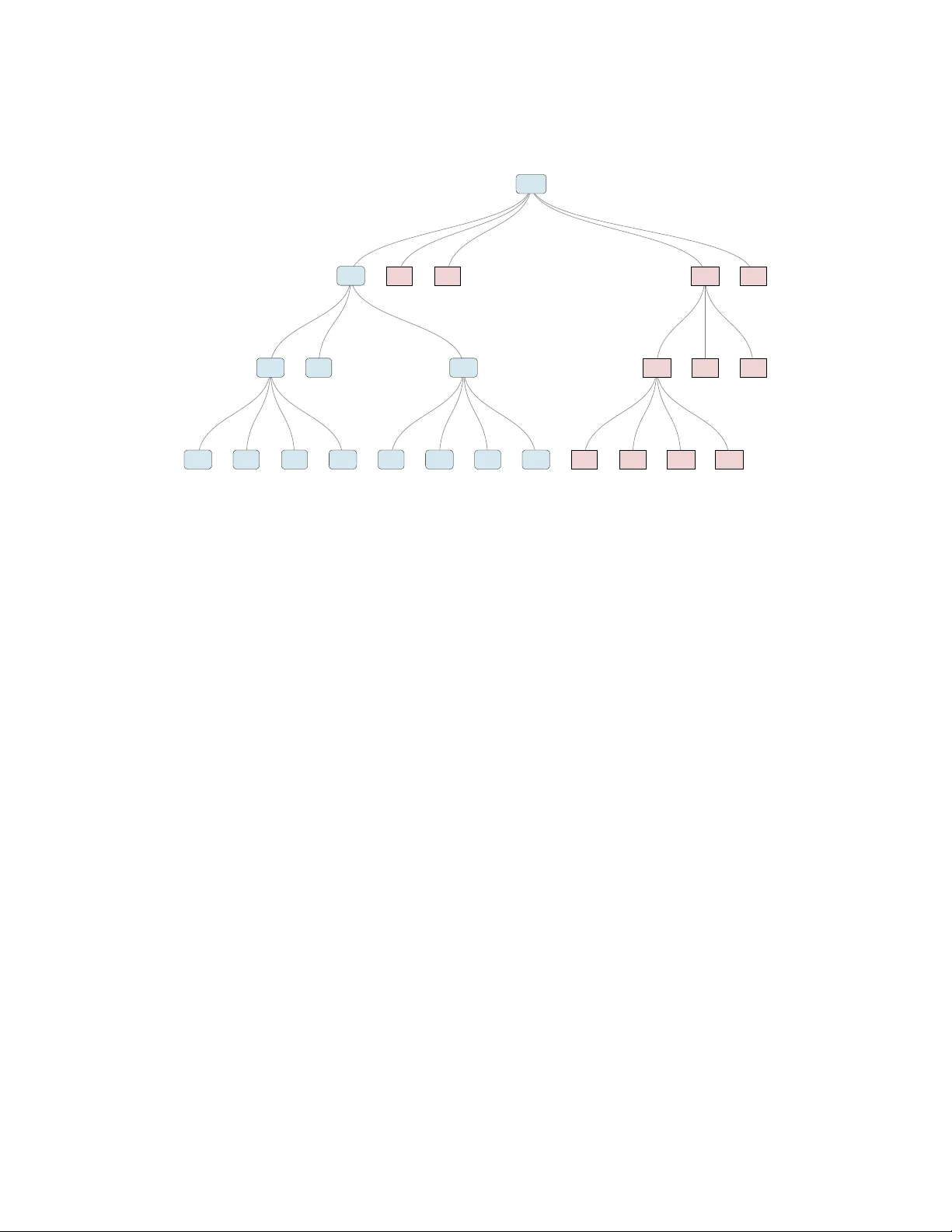
Detecting Where Eects Occur by T esting Hypotheses in Order Jake Bowers ∗ David Kim † Nuole Chen ‡ February 25, 2026 Abstract Experimental evaluations of public policies often randomize a ne w intervention within many sites or blocks. After a report of an overall result — statistically signicant or not — the natural question from a policy maker is: where did any ee cts occur? Standard adjustments for multiple testing pr ovide little p ower to answer this question. In simulations modeled after a 44-block education trial, the Hommel adjustment — among the most powerful proce dures contr olling the family-wise error rate (FWER) — detects eects in only 11% of truly non-null blocks. W e develop a procedure that tests hypotheses top-down through a tree: test the overall null at the root, then groups of blocks, then individual blocks, stopping any branch where the null is not rejected. In the same 44-block design, this approach detects eects in 44% of non-null blocks — roughly four times the detection rate. A stopping rule and valid tests at each node suce for weak F WER control. W e show that the strong-sense F WER depends on how rejection probabilities accumulate along paths through the tree. This yields a diagnostic: when power decays fast enough relativ e to branching, no adjustment is needed; other wise, an adaptive α -adjustment restores control. W e apply the method to 25 MDRC education trials and provide an R package, manytestsr . 1 Where do blo ck-level ee cts occur? Consider a block-randomized experiment with 44 experimental blocks such as the Detroit Promise Program (Ratledge et al. 2019) where treatment was assigned to students of dierent academic cohorts by ve community colleges. The overall test rejects the null of no ee cts. The policy-maker considering changes across all of Detroit’s community colleges now asks: where did the eects occur? W ere they concentrate d in a few sites, or spread ev enly? The answer determines whether to replicate the inter vention everywhere or investigate why it succeeded in some places and faile d in others. ∗ Political Science and Statistics, University of Illinois @ Urbana-Champaign, † Statistics, University of Illinois @ Urbana-Champaign ‡ MI T GO V/LAB, 1 A natural statistical response — test the null hypothesis of no eects in each blo ck separately , then adjust for multiplicity — is disappointing. In data w e simulated to follow the design of the Detroit Promise Program, the Hommel adjustment, one of the most p owerful procedures that controls the family-wise err or rate (FWER), dete cts eects in only 11% of the blocks that truly have them. The analyst reports “not enough information, ” and the policy-maker gets nothing useful. This pap er presents a dierent approach. 1 Instead of testing every block and adjusting afterward — a bottom-up strategy — we test hypotheses top-down on a tree. W e begin with the overall null at the root. If rejected, we split the blocks into groups following the administrative structure of the experiment and test each group. If a group’s null is rejected, we split again and continue down to individual blocks. If a group ’s null is not rejected, we stop testing on that branch. In the same simulation, this structured appr oach detects eects in 44% of the truly non-null blocks while controlling the F WER at the nominal level — roughly four times the detection rate of the bottom-up alternative. T wo conditions drive this result. First, a stopping rule : test a child hypothesis only after rejecting its parent. Second, valid tests : each individual test controls its false positive rate at level α . W e show that tw o conditions suce for w eak FWER control — control when all null hypotheses are true . For strong control, we analyze how power decay from data splitting limits error accumulation through the tr ee and, when needed, apply an adaptive α -adjustment. This framework builds on the close d testing tradition of Marcus, Eric, and Gabriel (1976), Rosenbaum (2008) and the sequential structured testing of Goeman and Solari (2010), Goeman and Finos (2012), and Meinshausen (2008), which we extend to randomization-based inference in block-randomized experiments. Our extensions to this foundational literature are substantive rather than cosmetic. In genomic applications of tree-structured testing, the same data are analyzed at every no de, the analyst must impose the conditions for valid testing as assumptions, and F WER adjust- ments apply uniformly across the tree. Block-randomized experiments dier in ways that the existing frame work does not exploit. First, the experimental design guarantees valid tests at each node: randomization-based p -values have exact size control by construction. Second, testing subsets of blo cks is itself a form of data splitting — child tests use less data and so should not produce more e xtreme evidence than their parents — so pow er decays through the tree as sample sizes shrink at each split, creating a geometric damping of error along each path. W e derive an e xplicit expression for F WER as a function of these path-wise rejection probabilities (Proposition 1), which reveals that high power at the root can inate error rates at the next level while low power at de ep levels provides natural 1 W e focus on the family-wise error rate (F WER) rather than the false discovery rate (FDR). The FDR controls the expected proportion of false discoveries among rejections, which suits settings where rejecte d hypotheses will be validated in follow-up studies. The FWER controls the probability of any false rejection, which suits settings where r ejected hypotheses lead directly to policy action. When a school district decides to scale an intervention based on where eects were detected, a single erroneous claim can misdirect resources. FDR-oriented extensions of tree-structured testing are discussed in Section 5. 2 protection from false positive errors. This expression motivates an adaptive α -adjustment that is stringent wher e power is high and relaxed where power decay triggers the stopping rule and testing stops. This paper makes three contributions. First, we sho w that the condi- tions for tree-structured weak FWER control are satised by design in block-randomized experiments. Second, we derive the relationship between power decay and str ong FWER that makes adaptiv e adjustment possible. Third, we demonstrate that these ideas yield two- to six-fold more discov eries than standard adjustments in realistic multi-site trials (T able 5), with gains of an order of magnitude or more in wider trees (T able 4). For researchers working in policy evaluation, the practical implication is clear: in experiments with administrative structures, more can be learned about the welfare eects of a new policy than we might have imagined without testing hyp otheses in order . T wo traditions of research address heterogeneous treatment eects. One estimates condi- tional average treatment eects as functions of obser ved covariates (e.g. W ager and Athey 2018; Hahn, Murray , Car valho, et al. 2020). The other studies the distribution of individual eects directly , asking how many units benete d and by how much (e.g. Heckman, Smith, and Clements 1997; Kim et al. 2025). Our work is closer to the se cond tradition: rather than asking which covariates moderate eects, we ask which experimental blocks or groups of blocks show dete ctable eects. Where covariate-based approaches focus on columns of the data matrix, we focus on rows — the sites, cohorts, and scho ols where eects did or did not occur . The approaches are complementary; detections could guide subsequent covariate-based investigation of why eects vary . W e focus on blo ck-randomized experiments with two treatment arms and roughly contin- uous outcomes. The results generalize to binary outcomes and multi-arm trials directly , although we do not engage those designs in our simulations or application. The paper proce eds as follows. Section 2 develops the b ottom-up and top-down testing approaches, pro ves w eak FWER control (Theorem 1), and illustrates the performance of the procedure using simulations across a wide range of tree sizes. Section 3 addresses strong F WER control by analyzing how pow er de cay thr ough the tree naturally limits err or accumulation, and develops an adaptive α -adjustment for settings where this natural gating is insucient. W e then demonstrate the method on data simulated to follo w the Detroit Promise Program design (Section 3.2) and apply it to 25 blo ck-randomized education trials elded by the MDRC (Diamond et al. 2021). 2 2 T esting to Detect Eects in Blocks Block-randomized experiments allow two styles of testing procedures that target blo ck- specic causal eects. In a study like that sho wn in Figure 1, we have a set of blo cks, B , 2 In the supplement we de velop a test statistic sensitive to distributional dierences bey ond mean shifts, so that eects that are positive in some blocks and negative in others do not cancel at the root. This statistic draws on energy statistics (Székely and Rizzo 2013) and multivariate permutation tests (Strasser and W eb er 1999; Hothorn et al. 2006). 3 within which a new policy inter vention is randomly assigned to m b people, leaving n b − m b in the status quo. Notice the inverted tree-like shap e of the experiment. The individual blocks ar e on the bottom of the tree and, in this case , ar e neste d within administrative units like cities and states toward the top of the tr ee. Overall State 1 City 1 B 1 B 2 B 3 B 4 . . . . . . . . . State 2 . . . . . . . . . State 3 . . . . . . City 20 B 98 B 99 B 100 Figure 1: An administratively organize d structure of blocks. A study randomly assigns people within oces ( B ) to a new intervention. Each oce is an experimental block containing m b people assigned to the inter vention and n b − m b people assigned to the status quo. 2.1 T esting in every block: the basic problem of multiple testing Since each block contains multiple units assigned at random to treatment, an analyst could treat each block as a mini-experiment (Gerber and Green 2012, Chap 3). With 100 blocks, we could execute 100 tests of the null hypothesis of no treatment eects. W e should also adjust the rejection criteria for those tests to protect the decision-makers from making too many false positive errors. Why adjust? Imagine that, in fact, there were no ee cts in any of the 100 blocks. If the tests are independent of one another , and we hav e set our rejection threshold at α = 0 . 05 , then we know that the probability that at least one of the 100 unadjusted tests would yield a statistically signicant result, p < 0 . 05 , in error is: P ( at least one p < 0 . 05) = (1 − (1 − 0 . 05) 100 ) ≈ 0 . 99 . That is, if we did a test in each of the 100 blocks in an experiment in which no ee cts occurred in any block, we would virtually certainly reject this null in one or more blocks — and make an error when we interpret this r ejection of "no eects" in those blo cks as implying some true causal eect occurred in those blo cks. This error rate of a colle ction of tests is often called the Family-wise Error Rate (FWER), and it can be controlled by an adjustment. For example , the Bonferroni adjustment suggests that if we refuse to reject the null hypothesis unless α adjusted = p ≤ 0 . 05 / 100 = 0 . 0005 , then we will have controlled the F WER because P ( at least one p < 0 . 05) = (1 − (1 − 0 . 05 / 100) 100 ) ≈ 0 . 05 (Lehmann and Romano 2005). 3 Of course, this approach makes it much harder to dete ct ee cts when they are actually 3 T echnically speaking, this explanation shows that dividing the rejection threshold by the numb er of tests, controls the FWER in the “weak sense" , which means it controls the FWER when there are no eects in any block. W e will discuss strong and weak control of the FWER later in the paper . 4 present. For example, the power of a t-test to dete ct an eect of 0.8 standard deviations within a block of 50 units is 0.79 when α = 0 . 05 and nearly half that power (power=0.46) when α = 0 . 005 . Structured approaches to testing can increase this p ower while controlling the F WER. 2.2 Sequential Structured T esting and W eak Control of the F WER Figure 1 shows that each experimental block is nested within a hierarchy . When hyp otheses are neste d in this way , they can be tested in a specic order under rules that avoid the sever e power loss of bottom-up adjustments. This insight originates in the “closed testing” framework of Marcus, Eric, and Gabriel (1976), dev eloped for structured experiments by Rosenbaum (2008) and Small, V olpp, and Rosenbaum (2011). W e build esp ecially on the general rules for se quential nested testing articulated by Go eman and Solari (2010) and Goeman and Finos (2012) and Meinshausen (2008). W e explain the reasoning behind the structured testing approach here b efore turning to formal dev elopment, simulations, and application. The general idea is to start testing hypotheses at the “r oot” of the tree — testing rst the null hypothesis of no eects in any block. If we can reject that hypothesis then we know either (1) that at least one blo ck contains at least one unit with a non-zero treatment eect or (2) that we hav e just made a false positive err or . This rst test could be the same test that anyone analyzing a block-randomize d e xp eriment might use — for example a block-aligne d t-test or rank-based Wilcoxon test. 4 The second and subse quent tests occur “lower” in the tree on subsets of the data split into disjoint groups. Once a test does not reject a hyp othesis, testing stops on that branch of the tree . W e prove that this pr ocedure controls the FWER when all null hypotheses are true (Theorem 1) and conrm the result via simulation across a wide range of tree sizes (T able 1). Conditions for F WER control T o x ideas, consider the tree in Figure 2. W rite H i for the null hypothesis of no treatment ee cts among any of the units in the blo cks descended from node i . At the root, H 1 is the hypothesis that no unit in any block has a tr eatment eect. At a leaf — no des 5 through 13 in the gure — H i pertains to a single experimental block. W e write p i for the p -value from the test of H i . node 1 node 2 node 3 node 4 5 6 7 8 9 10 11 12 13 Figure 2: A k -ary tree with k = 3 nodes per level and L = 3 levels and k L − 1 = 9 terminal nodes or “leaves" representing individual e xperimental blocks. 4 W e discuss test statistics in Supplement C. This project led us to develop two approaches to assessing the hypothesis of no eects that are immune from positive versus negative eect cancelation problems. W e defer the test-statistic development to the Supplement and focus here on the tree-structured testing procedure . 5 W e state two conditions. T ogether they suce for weak F WER control (Theorem 1). Combined with an analysis of power decay and, when ne eded, adaptive α -allocation, they also provide str ong control (§ 3). Condition 1 ( Stopping rule). A hypothesis H i is tested only if every ancestor of node i has b een rejected. If the root hypothesis is not rejecte d, no further tests are performed. If any hypothesis on a path from root to leaf is not rejecte d, no descendant on that branch is tested at all. In Figure 2, we do not test H 5 unless we have rejecte d both H 2 and H 1 . This condition distinguishes our procedure from tree-structured testing frameworks that test every no de and then determine which rejections to keep (Goeman and Solari 2010; Goeman and Finos 2012) and connects with frameworks for strictly nested testing that would focus on a single branch of a tree (Rosenbaum 2008). Our procedure may test only a small fraction of the tree ’s no des — and each untested node is a test that cannot produce a false positive. Condition 2 ( V alid tests). Each test at a node, if executed on its own, has a false positive rate no greater than α . In block-randomized experiments, randomization-base d tests satisfy this by design: permuting the treatment assignment within blocks produces p -values with guaranteed size control (Rosenbaum 2002, Chapter 2). These conditions enable us to state and prov e the following theorem: Theorem 1. Conditions 1 and 2 suce for weak F WER control A family of true null hypotheses organize d on an irregular or regular k -ary tree and tested following the stopping rule (Condition 1) with valid tests at each node (Condition 2) will produce a family-wise error rate (F WER) no greater than α . W e call a k -ary tree “regular” if the number of child nodes of a parent is the same for all no des in the tree. A k -ary tree is “irregular” if the number of child no des of a parent node may dier within and across levels of the tree. The proof of Theorem 1 is in Appendix A in the Supplement. W e pro vide some intuition here. Figure 3 sketches the algorithm that follows those rules while adding the idea of splitting the blo cks into groups. Data splitting will be important when we engage with strong control of the F WER, but is not necessary for weak control as we show in the proof and in the simulations below . In this version we talk about “splitting” the blocks as a way to speak in general ab out testing hypotheses on subsets of blo cks: we do not propose to split within blocks, just to divide the experimental blo cks into groups of blocks. In the example of the administrative structure above the “splits” ar e xed by design. In Figure 3 we write B 1 to refer to the set of all the experimental blo cks in the study — the set of blocks containing the units relevant to the hyp othesis at node 1, H 1 — and B 2 and B 3 for mutually exclusiv e subsets of blocks nested within B 1 (which could b e individual blocks that cannot be further split or groups of blocks which could be divide d). W e write B 4 for the rst subset of the B 2 set and so on. For simplicity in this paper we only test 6 the null hypothesis of no eects. At the level 1 or the root level, we test the null of no eects for any unit in any block and produce a p -value as the output of this test that we call p node 1 ≡ p 1 for “ p -value for the node 1 hypothesis” or “ p -value for the hypothesis that the potential outcomes for all units in all blocks under treatment are the same as the potential outcomes under control, H 0 : y i,b, 1 = y i,b, 0 ∀ i, b ∈ B 1 . ” If we cannot reject this overall null, such that p 1 > α , then testing stops. If we can reject the overall null, then at least one unit in one blo ck has a causal ee ct, we split the data into subsets and do further tests as shown in Figure 3. Given test result fr om B 1 , p 1 Stop Stop p 2 Split B 1 p 3 Stop Split B 2 Split B 3 p 3 p 5 p 6 p 7 Split B 4 into {B 8 , B 9 } Stop Stop Split B 7 into {B 14 , B 15 } if p 1 > α if p 1 ≤ α if p 2 ≤ α if p 2 >α or |B 2 | =1 Use B 2 to produce p 2 Use B 3 to produce p 3 if p 3 ≤ α if p 3 >α or |B 3 | =1 B 4 B 5 B 6 B 7 p 4 ≤ α |B 5 | = 1 p 6 > α Figure 3: Simplied ow of the T op-Down T esting and Splitting Algorithm with xe d false positive lev el α . All blocks are in set B 1 , B 2 is a subset of B 1 , B 4 is a subset of the blocks in B 2 . The p -value, p 1 , is the result from a test of the hyp othesis of no eects using all the blocks (i.e using the set B 1 ), p 2 is the p -value from a test of the null of no eects using only the blocks in B 2 . T esting stops when p > α or when the number of blocks in B , written |B | , is 1 such that for a given node i , |B i | = 1 . The intuition for the proof of Theorem 1 arises from the fact that in a randomized experi- ment, w e know that the pr obability of a false positive error in a single randomization-based test is low and controlled: the size is less than or equal to the level ( α ). This is stated as a condition of the proof in Condition 2. Another way to say this: if the null of no eects is true in all blocks, then we should reject the root hypothesis with probability less than α . An incorrect rejection thus happ ens with very low probability and so rarely are other tests even done, and when they ar e done their own false positive rates are less than or equal to α . The simulation results in T able 1 show control of the F WER for a wide range of tree sizes and congurations when there are no tr eatment eects. 2.2.1 Simulation Study of W eak Control of the FWER to Illustrate the Proof Given a spe cication of a complete k -ary tree using k nodes per lev el and L levels we drew p -values from uniform distributions. The valid tests condition (Condition 2) implies that the distribution of p -values across tests of the true null should b e stochastically dominate d by the uniform (Lehmann and Romano 2005, Chapter 3). That is, in many tests of a true 7 null hypothesis, only 5% of p -values should be less than p = 0 . 05 , 10% should be less than p = 0 . 1 , etc. . . . 1. For the root node, draw p 1 ∼ U (0 , 1) ; a draw which r espects the valid test condition such that P ( p 1 ≤ α ) ≤ α in this case. 2. If p 1 ≤ α , draw p l =2 ,k independent p -values from U (0 , 1) for the k -nodes at level 2. 3. For any of the k p -values at level 2 where p l =2 ,k ≤ α , generate p -values for its children with U (0 , 1) . For any p l =2 ,k > α , stop testing in the branch of the tree that would descend from that node. This implements the stopping rule condition (Condition 1). 4. Continue testing, drawing from uniform distributions for child nodes with parents with p ≤ α , descend into the tree towards the leaves, and stop testing in any branch when p > α or when the node tested is a leaf. In this simulation we did not represent the idea of data splitting or any other adjustments. So, these results are much more optimistic than they would b e if, in fact, the sample size used to test a hypothesis at level 2 is less than that available at the root node. For each tree , we repeated this procedure 10,000 times, recording whether any of the p -values in the tree of true null hyp otheses were ≤ α . The proportion of simulations with at least one such false rejection is a measure of the FWER. T able 1 shows the r esults. Whether the tree has k = 2 nodes per le vel or k = 100 , the rules lead to a maximum FWER within simulation error . 5 A tree with k nodes per level and a maximum of L levels has k ℓ − 1 nodes at level ℓ and k L leaves. The rst row of the table shows binary trees ( k = 2 ): with 2 levels we hav e 4 leaves and 7 total nodes; with 18 levels we have 262,144 leaves and 524,287 total nodes. This set of simulations produces research designs that tend to be unrealistic from the perspective of block-randomize d experiments in public policy — rarely would one have 260,000+ experimental blocks! But these extreme examples provide what w e hope is a compelling illustration of Theorem 1. T able 1 also shows that the two rules lead the algorithm to nearly always stop after testing the single root node: the average numb er of tests is close to 1, even when the tree has hundreds of thousands of no des. In contrast, the bottom-up procedure must execute a test in every block and then adjust the r esults — thousands of tests wher e the top-down procedure does one (Hommel 1988). 2.2.2 Why might weak control suce? The simulations and proof above assume that no units in any blocks have tr eatment eects — that all null hyp otheses are true. This is what it means for a proce dure to control the 5 Whether we use 2 × p 0 . 05(1 − 0 . 05) / 10000 = 0 . 004 or 2 × p 0 . 5(1 − 0 . 5) / 10000 = 0 . 01 we interpr et these results to show nominal FWER control. 8 Levels Max A vg. Max Nodes Leaves k Min Max F WER T ests Min Max Min Max 2 2 18 0.052 1.008 7 524287 4 262144 4 2 8 0.055 1.015 21 87381 16 65536 6 2 6 0.054 1.026 43 55987 36 46656 8 2 6 0.050 1.032 73 299593 64 262144 10 2 4 0.049 1.044 111 11111 100 10000 20 2 4 0.050 1.202 421 168421 400 160000 50 2 2 0.048 1.402 2551 2551 2500 2500 100 2 2 0.050 2.498 10101 10101 10000 10000 T able 1: This table shows weak-control of the family-wise error rate acr oss 10,000 simula- tions ( estimate d simulation error = .01) using α = . 05 on k -ary trees with k nodes per le vel where the hypothesis of no eects is true for all nodes. Each ro w summarizes the results of simulations for the trees with a given k and between the minimum and maximum numb er of levels for that number of nodes per level. Maximum average false positive rates across the 10,000 simulations are sho wn in the ‘Max FWER’ column. The maximum number of nodes tested are shown in ‘Max T ests’ . And information about the range of trees is also shown: the total number of nodes in the trees and the total number of terminal nodes or leaves. F WER “in the weak sense ” (Ho chberg and T amhane 1987). The next section dev elops conditions for strong FWER control, which holds regardless of which hypotheses are true. Y et Conditions 1 and 2 on their own may b e appropriate for some research settings, and the reasoning is worth making e xplicit. A useful point of comparison is the Benjamini–Ho chberg procedure (Benjamini and Hochberg 1995), the standar d tool for controlling the false discovery rate (FDR) — the expected proportion of false rejections among all rejections. Benjamini and Hochb erg (1995) prov ed that their procedure controls the FDR at level α regardless of which hypotheses are true and which are false. Y et when all null hypotheses are true, ev ery rejection is a false rejection, so FDR equals FWER; the procedure therefore controls the FWER in the weak sense but not in the strong sense. Researchers accept this because FDR control suits ex- ploratory settings wher e ndings will b e validated in follo w-up studies. The tree-structured approach does not control the FDR (developing such guarantees is b eyond the scope of this paper), but it shares with FDR procedures the property that the F WER is controlled at α when all null hypotheses are true. The choice among error-rate guarante es depends on the research question. Does this program work at all? prioritizes detecting any eect over pinp ointing which specic outcomes are aected; weak F WER control suits this goal. Because the gate absorbs the entire multiplicity cost, every downstream test runs at nominal α — p ower that both strong F WER and FDR methods sacrice for their broader guarante es. Which individual outcomes are aected? — where each claimed detection must stand on its own — calls for strong F WER control. FDR pr o cedures occupy a middle ground, accepting that the list of discoveries may contain false entries but limiting their proportion. For the rst question, the tree-structured 9 procedure is a natural t: the overall test serves as a gate , and Conditions 1 and 2 make the weak FWER guarante e explicit. Researchers who are using the tree-structured approach to screen blocks for closer exami- nation can work with Conditions 1 and 2 alone. But in many applied settings, researchers want to make claims ab out spe cic blocks with the same error-rate guarantees they would demand of any conrmatory analysis. The next section shows how: analyzing the power decay inherent in data splitting — and, when needed, applying adaptive α -allocation — yields strong FWER control while preserving the power advantage of top-down testing. 3 Strong contr ol of the FWER Conditions 1 and 2 control false positive errors when all null hypotheses are true. Control of the FWER when at least one block contains a non-zero tr eatment eect — strong control — requires additional structur e. The key quantity turns out to be the power of the test at each node: the probability that the procedure both reaches a null node and then rejects it depends on the sequence of rejection probabilities along the path from root to that node. T o x ideas, consider the small tree in Figure 4: a k -ary tree with k = 3 children per node, L = 3 levels. A complete k -ary tree has k L − 1 leaves, so this tree has 3 2 = 9 leaves or experimental blocks and 13 total no des. W e develop our theor y using complete k -ary trees for simplicity , though the applications use irregular trees. In the gure, the causal eect is non-zero only in blo ck 5 ( boxed). Because blo ck 5 has a non-zero eect, its ancestors — nodes 2 and the root — are also non-null. So 3 of the 13 no des are non-null and 10 are null. 1 2 3 4 5 6 7 8 9 10 11 12 13 Figure 4: A k -ary tree with k = 3 and L = 3 . Boxes sho w non-null nodes: since the leaf (node 5) is non-null, all of its ancestors are non-null. The other nodes in the tree are null. Notice that the probability of making a false positive error in this tree dep ends on whether the hypothesis of no eect on a null node like node 3 or 13 is (1) tested and (2) rejecte d (w e are using "null node " as a short hand for "node with no causal eect" or "node where the hypothesis of no ee cts is true"). Figure 4 contains a tree where we want to reject the root node. In fact, we should reject that node with probability much greater than α if we have enough data and the causal eect aggregated to that node is large. This line of reasoning rev eals that the probability of false positive errors dep ends on the power of the test at the root node (w e write the statistical power of a test at node i as π i ). Consider two extreme cases: (1) the overall test has very low power and (2) it has very 10 high power . If the overall test has ver y low power , say π 1 ≤ α , then this test will reject very rarely , and, in turn, the tr ee will show very few false positive errors. In fact, if π i ≤ α , then the two conditions use d above control the F WER in the strong sense: not rejecting at the root controls the FWER whether the lack of rejection is be cause all blocks have no eects and the test has false positive error rate of less than α or because at least one blo ck has a non-zero eect but the test lacks the power to detect that eect ( π 1 < α ). What about when π 1 > α ? In this case, the multiple testing of null nodes are no longer protected by the root. For example, in Figure 4 rejection of the root will lead to 3 tests, two of them of null nodes. W e will have two chances to falsely reject the null of no ee cts and, if the tree stopped with nodes 2,3 and 4, the F WER would be greater than α without further assumptions. 3.1 Strong control via error load and adaptive adjustment Our approach exploits the tree’s gating structure. W e show in Proposition 1 in the Sup- plement that the probability of a false p ositive error at any node is determined by the probability that the procedure both reaches that node and then rejects it. Let H 0 denote the set of indices i for which H i is true, and dene the conditional rejection probability θ j at node j as α j (the test size) when H j is true, or π j (the power) when H j is false — in both cases conditional on all ancestors of j having been rejected. W rite anc ( i ) for the set of proper ancestors of node i (e xcluding i itself ). And let R i = I { reject H i } : the rejection indicator at no de i . Under the Stopping Rule, R i = 1 requires that R j = 1 for every j ∈ anc ( i ) . Then the F WER satises FWER = P   [ i ∈H 0 { R i = 1 }   ≤ X i ∈H 0 α i Y j ∈ anc( i ) θ j , (1) and we dene the product ov er an empty set of ancestors (for the root node) to be 1 . Corollary 2 shows how this e xpression recov ers weak FWER control when the root has very low power ( π 1 ≤ α ): the root itself rarely rejects, so no descendant is teste d. The expression also r eveals the problem when the r o ot has high p ower — the scenario we pr efer . When π 1 = 1 , rejection at the root is certain, and the F WER at level 2 is approximately k · α 2 , the sum of the false p ositive rates across all k children in that rst branch of the tree from the root. With 10 children each tested at α = 0 . 05 , the F WER reaches 0 . 5 . T o build intuition, imagine that the root has p erfect power ( π 1 = 1 ) and that the blo cks are split into k equal-sized groups at each level. Be cause each group contains 1 /k of the data, the test at each child node has lower power than its parent: if we approximate power using the Normal distribution, θ ≈ Φ( ˆ δ p N node / 4 − z α/ 2 ) , then halving the sample size at each split reduces power geometrically . At level ℓ , the tree has k ℓ − 1 nodes, and each null 11 node is reached only if every ancestor on its path rejected. The product of these rejection probabilities along the path from the root determines how likely the procedure is to reach — and therefore to falsely r eject — each null node. W e formalize this as the error load at level ℓ : G ℓ = k ℓ − 1 Q ℓ − 1 j =0 θ j , which is the product of the number of no des at level ℓ and the probability that the procedure reaches that level (see Appendix B, Supplement). The error load measures how many null nodes at each lev el are exposed to testing. When the total error load P L ℓ =1 G ℓ ≤ 1 , the F WER contribution from all levels combined stays below α , and the unadjusted procedure controls F WER (Theorem 2). W e call this natural gating : power decays as data splitting reduces sample sizes at each level, and this de cay limits how many null nodes the procedure can reach. In the multi-site education policy trials that motivate this pap er — moderate eect sizes, k ≈ 3 , L ≈ 3 — the error load is typically below 1 and no adjustment is needed. When the error load excee ds 1 — as it will with wide trees, shallow depth, or high root power — we de velop an adaptiv e α -adjustment in Appendix B.4 (Supplement). If the test statistic has an asymptotically Normal distribution — Appendix C (Supplement) introduces one that does, following Hothorn et al. (2006) — then we can compute power at each depth before testing begins and adjust α accordingly (Remark 8 and Theorem 4) as follows: α adj ℓ = min ( α, α k ℓ − 1 · Q ℓ − 1 j =1 ˆ θ j ) (2) W e derive this expression for regular k -ary trees where each node has k children. For irregular trees — where the numb er of children varies across no des — the error load at each depth becomes a sum o ver the actual nodes at that depth, G ℓ = P i ∈ level ℓ Q j ∈ anc ( i ) ˆ θ j , and the adjusted α at depth ℓ is min { α, α/G ℓ } . The manytestsr R package implements this general formula via alpha_adaptive_tree() , which accepts a table of node sizes and computes per-depth power estimates for arbitrary tree structures. The practical implication is that adjustment should be stringent near the root, wher e pow er is high and many null siblings are expose d, and relaxed at deep er levels, where p ower decay already gates the procedure. This resembles alpha-investing (Foster and Stine 2008), but here the investment schedule is determined by the relationship between power and tree structure rather than by observed p -values. 3.1.0.1 Branch pruning. The adaptive adjustment of Equation (2) computes the error load from the full tree b efore any testing begins. But when a branch fails to reject at depth ℓ , the entire subtree below it is pruned: those nodes will never b e tested, and the null sibling groups they would have contributed to de eper levels vanish from the error load. Branch pruning exploits this by recomputing the adaptive α -schedule on the surviving subtree after each depth. When one of k branches at depth 1 survives, the error load at depth 2 drops by a factor of roughly k , and the adjuste d α at deep er levels increases 12 correspondingly . The gain is largest in wide trees where most branches are null — exactly the setting where the pre-computed adjustment is most conservative. 6 3.2 An Example: A Simulate d V ersion of The Detroit Promise Program The Detroit Promise Program (DPP) (Ratle dge et al. 2019) involved enhanced advising, nan- cial support, and encouragement of full-time enrollment to community college students in an eort to increase graduation rates. The trial randomized this bundle of treatments within ve community colleges in the Detroit area: Henry Ford Community College, Macomb Community College, Oakland Community College, Schoolcraft College, and W ayne County Community College District. Each college elded the trial for 3 academic year cohorts, and within the cohorts students were further subdivided into 1 to 4 experimental blocks within which the intervention was randomly assigned. T o illustrate the algorithm, we generated a design that preser ved the DPP structure — 5 college no des under the ov erall node with varying numb ers of cohorts and sub-cohort blocks, for 44 blo cks total — but diered in ways that facilitated simulation. Every blo ck had 50 students, and potential outcomes under control wer e drawn from N (10 , 9) to roughly match the observed distribution of credits taken, but with more variation. W e concentrated all non-zero eects in a single college: 9 blocks within HFCC have treatment eects while the 35 blo cks across the other four colleges are pure null. This concentration mimics a pattern common in multi-site trials and visible in the MDRC data (Section 4): eects that are localized within particular sites rather than uniformly spr ead. Each block contains 50 students. For the illustration w e use a large eect (Cohen’s d = 0 . 80 ) within each of the 9 blocks with non-null eects so that the root-lev el test rejects and the tr ee structure is visible; the simulation study that follows evaluates realistic eect sizes. Figure 5 shows the results of the structured testing approach with nodes that are truly non-zero displayed in blue. Any ancestor of a non-zero blo ck is itself non-zero — a rejection at the college or cohort level is a true discovery , not an err or . The algorithm teste d 18 of the 44 blocks rather than all 44, pruning branches roote d at colleges where the college-lev el test did not reject. It corr ectly identied HFCC as the source of treatment eects and descended into its cohorts and blo cks, detecting four of the nine non-null blocks while falsely r eje cting two of the 35 null blocks. 6 Note to the reader: W e are still working on the proof for branch pruning. W e present the simulations below which show it working, but this is a late breaking advance . 13 Overall # Blocks=44 p=0 HFCC # Blocks=9 p=0 Cohort 1 # Blocks=4 p=0 Cohort 2 # Blocks=1 p=0.091 Cohort 3 # Blocks=4 p=0 Block0080 # Blocks=1 p=0.019 Block0081 # Blocks=1 p=0.067 Block0082 # Blocks=1 p=0.206 Block0083 # Blocks=1 p=0.005 Block0085 # Blocks=1 p=0.536 Block0086 # Blocks=1 p=0.001 Block0087 # Blocks=1 p=0.052 Block0088 # Blocks=1 p=0.01 MCC # Blocks=8 p=0.905 OCC # Blocks=9 p=0.638 SC # Blocks=9 p=0.02 WCCC # Blocks=9 p=0.892 Cohort 1 # Blocks=4 p=0.001 Cohort 2 # Blocks=1 p=0.953 Cohort 3 # Blocks=4 p=0.966 Block0106 # Blocks=1 p=0.224 Block0107 # Blocks=1 p=0.514 Block0108 # Blocks=1 p=0.016 Block0109 # Blocks=1 p=0.016 Figure 5: Results of top-down testing in a simulation of 44 experimental blocks following the pre-specied experimental design of the Detr oit Pr omise Pr ogram (Ratledge et al. 2019). Nine blocks within HFCC have non-zero eects (Cohen’s d = 0 . 80 ); all other blocks are pure null. The algorithm identies HFCC and descends into its cohorts and blocks while pruning null colleges. Abbreviations: Henry Ford Community College (HFCC), Macomb Community College (MCC), Oakland Community College (OCC), Schoolcraft College (SC), W ayne County Community College District (W CC). Blue nodes have non-zero causal eects. This illustration shows that a policy maker seeking to identify which colleges or blocks showed treatment eects would nd the bottom-up approach disappointing: the Hommel (1988) adjustment across 44 blocks detects just one blo ck despite nine having genuine eects. The structured approach leads attention away from three of the ve colleges and identies not only more individual blocks but also higher-level groupings — the HFCC college itself — that can direct further exploration toward understanding why eects concentrated there . The gure also shows the cost of using no α -adjustment: Schoolcraft College (SC), a purely null college , rejected at the college lev el ( p = 0 . 020 ), and the procedure descended through SC Cohort 1 ( p = 0 . 001 ) to falsely reject two null blocks (Block0108 and Block0109, both p = 0 . 016 ). These false rejections illustrate the cascade that the adaptive α -adjustment of Equation (2) is designed to prevent. With adjustment, the SC college-level test would face a tighter threshold and would not r eject, eliminating the entire false-rejection chain. This is a single simulate d dataset with a large ee ct size chosen to make the tree structure visible. Power and error rates describe the behavior of a pr o cedure across repetitions of design. W e now turn to a simulation at realistic eect sizes but using r egular k -ary trees for simplicity to evaluate these properties systematically . 14 3.3 Does the approach control the FWER? W e used the same DPP design — 9 non-null blocks concentrate d in one college, 35 pure-null blocks across the other four colleges — but set the eect size near the me dian of the obser ved overall MDRC eect sizes (Section 4) at Cohen’s d = 0 . 20 for each of the 9 non-null blocks. So, this is a simulation with more power at the root than we would se e in those studies. W e repeated the simulation 10,000 times, re-randomizing treatment within each block while maintaining the same ee ct structure. Each iteration recorded whether a false positive error occurred at the level of individual blocks (“leaves”) or at any node in the tree . T able 2 summarizes the results. T est Characteristic 3 Rules + Loc. Hom. + Loc. BH + Adapt. α + Ad. α Pr . Nodes tested 3.983 3.350 3.484 3.077 3.521 Node F WER 0.028 0.005 0.005 0.005 0.009 Node False Rej. Prop. 0.018 0.003 0.003 0.003 0.006 Node Power 0.039 0.016 0.018 0.018 0.033 Leaves tested 2.447 1.989 2.098 1.776 2.120 Leaf Power 0.039 0.016 0.018 0.018 0.033 Leaf True Rejections 0.274 0.108 0.121 0.116 0.240 Leaf F WER 0.028 0.005 0.005 0.005 0.009 Leaf False Rej. Prop. 0.004 0.001 0.001 0.001 0.001 Bottom Up Power 0.004 0.004 0.004 0.004 0.004 Bottom Up True Rejections 0.033 0.036 0.038 0.037 0.035 Bottom Up F WER 0.024 0.022 0.028 0.022 0.023 Bottom Up False Rej. Prop. 0.001 0.001 0.001 0.001 0.001 T able 2: Operating characteristics of ve testing procedures across 10,000 simulations ( α = . 05 ) using simulated Detroit Promise Program data where 9 of 44 blocks (all in one college) have non-zero eects (Cohen’s d = 0 . 20 ). ‘No de’ refers to any test in the tree (internal or leaf ); ‘Leaf ’ refers to individual experimental blocks; ‘Bottom Up’ shows the at Hommel adjustment across all 44 blocks. ‘F WER’ is the proportion of simulations with at least one false rejection. ‘False Rej. Prop. ’ is the mean proportion of truly null hyp otheses falsely rejected per simulation. ‘Power’ is the mean proportion of non-null hypotheses correctly rejected. ‘True Rejections’ is the mean number of non-null hypotheses rejected. Boldface marks values discussed in the text. T able 2 compares ve top-down variants against a b ottom-up Hommel baseline. The columns represent dier ent combinations of the tools introduced above: “3 Rules” applies only the stopping rule and valid-test conditions (Conditions 1 and 2); “+ Loc. Hom. ” and “+ Loc. BH” additionally adjust p -values within each sibling group using the Hommel (1988) or Benjamini and Hochberg (1995) proce dure before comparison to α ; “+ Adapt. α ” uses the adaptive α -adjustment of Equation (2) ; and “+ Ad. α Pr . ” combines the adaptiv e α -adjustment with branch pruning — recomputing the α -schedule on the sur viving subtr ee after each depth, so that dead branches free up alpha for the remaining tests. Each row reports a dierent operating characteristic: F WER (the proportion of simulations with at least one false rejection), p ower (the proportion of non-null hypotheses correctly rejecte d), 15 and true rejections (the average number of non-null hypotheses rejected per simulation). The bottom three rows show the corresponding quantities for the at Hommel adjustment applied to all 44 blocks simultaneously . At d = 0 . 20 , the error load is 4.74 — well ab ove the threshold of 1 where Theorem 2 guarantees control. Y et the unadjusted two-conditions procedure still controls the FWER at 0.031, be cause the error-load condition is sucient but not necessar y: the DPP tree’s concentrated-eect structure provides additional natural gating beyond what the general bound captures. The adaptive α -adjustment (Equation 2) brings the F WER down further to 0.006. Bottom-up Hommel also controls the F WER (0.022) but at a ste ep cost: it dete cts eects in only 0.4% of the truly non-null blocks, compared to 3.9% for the unadjuste d top-down procedure and 2.0% for the adaptive variant. Although absolute power is low — realistic at d = 0 . 20 with N = 50 per block — the relative advantage is large. The unadjuste d structured approach averages 0.27 true leaf rejections per simulation, nearly eight times the bottom-up Hommel’s 0.035. Even the most conservative structured variant (adaptive α ) averages 0.13 true rejections, more than three times the bottom-up rate. Branch pruning improv es further: the pruned adaptive variant averages 0.24 true rejections — nearly twice the non-pruned adaptive rate — b ecause once the four null colleges fail to reject at depth 1, their subtrees vanish from the error load and the α -schedule relaxes for de eper levels within HFCC. At d = 0 . 30 , pruning yields 0.61 true rejections versus 0.21 for the non-pruned adjustment, a gain of 2 . 9 times. This advantage arises b ecause the top-do wn procedure aggregates signal at the college level ( N = 450 for HFCC) before descending to individual blocks, while the b ottom-up approach tests each block with less information — N = 50 — and pays a heavy multiplicity p enalty across all 44. Branch pruning amplies this advantage: when the procedure correctly identies HFCC as the active college and prunes the four null colleges, the eective tree narrows fr om 5 branches to 1 and the error load drops accor dingly . The table also shows two lo cal-adjustment variants. The “plus Lo cal Hommel” column applies a Hommel adjustment to the children of each internal no de: leaf power drops from 0.040 to 0.015 and the F WER from 0.031 to 0.004. The “plus Local BH” column applies the Benjamini-Hochberg procedure locally: similar power (0.017) and F WER (0.005). These local adjustments provide additional conser vatism, but at d = 0 . 20 the unadjusted procedure already controls the FWER, and the prune d adaptive α achieves comparable FWER control (0.009) with the highest power among the adjusted variants (0.034). The DPP results illustrate a pattern that may hold broadly: the error-load condition of Theorem 2 is conservative, and the unadjusted procedure often contr ols the FWER even when the error load exceeds 1. But how far can this tolerance str etch? At d = 0 . 30 with the same DPP tree, the error load r eaches 8.85 and the unadjusted F WER rises to 0.039 — still below 0.05, but close. The adaptive α -adjustment provides insurance, holding the FWER at 0.003 with a power cost (leaf power dr ops from 0.098 to 0.031). Branch pruning recovers much of this lost power: the prune d variant achieves a FWER of 0.009 with leaf power of 16 0.079. In wider trees with stronger eects, the unadjuste d procedure will eventually inate beyond 0.05 and α -adjustment is necessary . W e now probe this boundar y with a simulation study that varies tree width, eect size, and the proportion of null hypotheses to create scenarios spanning error loads fr om 0.2 to 3.1. This design isolates the testing procedure from data-generation details, letting us identify where the unadjusted procedure breaks down and how much power the adaptive correction costs. 3.3.1 Simulation Study of Strong F WER Control The weak-contr ol simulation ab ove teste d trees under the global null, where every hy- pothesis is true. W e now study how the proce dure behaves when some hypotheses are false — the setting in which strong F WER control matters. The central question is whether the unadjusted top-down procedure inates the FWER when powerful root tests e xpose many null sibling groups to testing, and whether the adaptive α -adjustment of Equation (2) corrects the ination. W e consider two tree structures: binary ( k = 2 , depth 3, yielding 8 leaves) and quaternar y ( k = 4 , depth 3, yielding 64 leaves). For each tree we var y the eect size and the proportion of null hypotheses, creating 14 scenarios in total. W e express eect sizes as Cohen’s d — the same planning parameter used to calibrate the adaptive α -adjustment. Three values calibrate three p ower regimes: d = 0 . 04 yields root p ower of appr oximately 0.15 (error load well below 1, natural gating suces); d = 0 . 10 yields root power of approximately 0.61 (err or loads near the transition threshold); and d = 0 . 15 yields root power of approximately 0.92 (err or load above 3, the regime where we expect the unadjusted procedure to inate). Each eect size is crossed with two null proportions: 80% null (the worst case for ination, since many null sibling groups are exposed) and 50% null. T wo additional all-null scenarios ( k = 2 and k = 4 ) verify that all methods contr ol the FWER when every hypothesis is true . For each scenario, we draw p -values rather than simulating raw data, isolating the testing procedure from data-generation details. Non-null leaves receive p -values drawn from Beta ( a, 1) , where the shape parameter a is calibrated so that the rejection probability matches the power implied by Cohen’s d and the sample size available at that leaf. Null leaves receive p -values from U (0 , 1) . Parent and child p -values are drawn independently given each no de ’s null status; the procedure does not r e quire monotonicity b etween parent and child p -values (see Remark 9 in the Supplement). W e compare seven methods organized into two families: T op-down, unadjusted (TD-Unadj). The basic gating procedure of Section 2, testing each node at the nominal α = 0 . 05 with no lo cal multiplicity adjustment. T op-down, Hommel (TD-Hommel). Same gating rule, but within each sibling group the p -values are adjusted by the Hommel procedure before comparison to α . 17 FWER k d Null P G TD TD-Hom TD- Adp TD-A -H TD-A -Pr BU-Hom BU-BH 2 0.04 50% 0.2 0.000 0.000 0.000 0.000 0.000 0.024 0.026 2 0.10 50% 1.2 0.009 0.004 0.011 0.003 0.014 0.026 0.031 2 0.15 50% 3.1 0.042 0.020 0.016 0.007 0.037 0.024 0.034 2 0.04 80% 0.2 0.005 0.002 0.005 0.001 0.007 0.044 0.045 2 0.10 80% 1.2 0.034 0.018 0.028 0.013 0.033 0.042 0.044 2 0.15 80% 3.1 0.075 0.056 0.035 0.023 0.053 0.045 0.050 2 — 100% 1.2 0.050 0.051 0.052 0.052 0.051 0.051 0.052 4 0.04 50% 0.2 0.001 0.000 0.000 0.000 0.001 0.027 0.028 4 0.10 50% 1.3 0.014 0.001 0.004 0.000 0.011 0.021 0.022 4 0.15 50% 3.1 0.057 0.003 0.004 0.000 0.026 0.024 0.026 4 0.04 80% 0.2 0.001 0.000 0.001 0.000 0.003 0.040 0.042 4 0.10 80% 1.3 0.023 0.001 0.008 0.000 0.030 0.041 0.043 4 0.15 80% 3.1 0.115 0.009 0.010 0.001 0.054 0.041 0.043 4 — 100% 1.3 0.048 0.050 0.049 0.052 0.047 0.047 0.048 T able 3: Strong FWER control across 14 scenarios and 7 methods (10,000 simulations per cell; simulation error ≈ 0 . 010 ). TD = top-down with nominal α = 0 . 05 ; Hom = local Hommel adjustment within each sibling group; Adp = adaptive α -adjustment (Equation 2); A -H = both adaptive and Hommel; A -Pr = adaptive with branch pruning; BU-Hom/BH = bottom-up Hommel/Benjamini–Hochb erg applied to all leaves. Boldface indicates F WER exceeding α plus simulation error . d = Cohen’s d (eect size); Null = proportion of null hypotheses; P G = total error load. All-null rows (100% null) use a placeholder eect size. T op-down, adaptive (TD-A dapt). The gating pr ocedure with α -levels adjuste d by Equa- tion (2), using estimated power at each depth. No local adjustment. T op-down, adaptive + Hommel (TD- Adapt-Hom). Both adaptive α -adjustment and local Hommel correction. T op-down, adaptive prune d (TD- Adapt-Pr). The adaptive α -adjustment with branch pruning: after each depth, the error load is recomputed on the sur viving subtree and the α -schedule for deep er levels is updated. Bottom-up, Hommel (BU-Hommel). All leaves are tested simultaneously , with the Hommel procedure applied globally . Bottom-up, BH (BU-BH). All leaves are teste d simultaneously , with the Benjamini– Hochberg proce dure applied globally . For each of the 14 scenarios and 7 metho ds, we repeat the procedure 10,000 times. Within each scenario, all v e top-down methods use the same random se ed, so they operate on identical trees and leaf p -values. W e record the F WER (the proportion of simulations in which at least one true null hypothesis is rejected) and p ower (the proportion of non-null leaves correctly rejected, averaged across simulations). T able 3 reports the F WER for all seven methods across the 14 scenarios. T able 4 compares the number of true discoveries b etween the adaptive top-down procedures (with and without branch pruning) and the bottom-up Hommel alternative. The rows labeled “—” in the d column of T able 3 are the all-null scenarios ( k = 2 and k = 4 with 100% null hypotheses). These rows ser ve as a sanity che ck: they reproduce 18 TD- Adp TD- A-Pr BU-Hom k d Null P G F WER Disc. F WER Disc. F WER Disc. Ratio 2 0.04 50% 0.2 0.000 0.16 0.000 0.17 0.024 0.02 7 × 2 0.10 50% 1.2 0.011 1.08 0.014 1.15 0.026 0.12 10 × 2 0.15 50% 3.1 0.016 2.69 0.037 2.90 0.024 0.31 9 × 2 0.04 80% 0.2 0.005 0.16 0.007 0.16 0.044 0.01 22 × 2 0.10 80% 1.2 0.028 0.83 0.033 0.85 0.042 0.03 33 × 2 0.15 80% 3.1 0.035 1.63 0.053 1.71 0.045 0.08 22 × 4 0.04 50% 0.2 0.000 0.17 0.001 0.19 0.027 0.02 8 × 4 0.10 50% 1.3 0.004 0.88 0.011 1.01 0.021 0.02 42 × 4 0.15 50% 3.1 0.004 1.92 0.026 2.19 0.024 0.04 54 × 4 0.04 80% 0.2 0.001 0.17 0.003 0.19 0.040 0.01 19 × 4 0.10 80% 1.3 0.008 0.87 0.030 0.99 0.041 0.01 108 × 4 0.15 80% 3.1 0.010 1.90 0.054 2.09 0.041 0.02 135 × T able 4: True disco veries and testing eciency: top-down adaptive (TD- Adp), top-down adaptive with branch pruning (TD-A -Pr), and bottom-up Hommel (BU-Hom) across 12 scenarios with non-null eects (10,000 simulations each). TD metho ds count correctly rejected non-null hypotheses at all levels of the tree; BU-Hom counts correctly rejecte d non- null leaves. Disc. = average true discoveries per simulation. Ratio = TD- A -Pr discoveries ÷ BU-Hom discoveries. Boldface F WER indicates ination b eyond α + simulation error . the weak-control setting of T able 1 within the strong-control simulation frame work. All methods control the F WER at the nominal level in these r ows, as expected. Three patterns emerge from these tables. First, when the total error load P G ℓ is at most 1 — the regime where Theorem 2 guarantees control — every method controls the F WER at or below the nominal level. The unadjusted top-down procedure, the adaptive variant, and both b ottom-up procedures all remain below 0.05. This conrms that natural gating works in the regime for which it was designed. Recall that the error load measures how many null nodes at each depth are exposed to testing: it is the product of the numb er of nodes at that depth and the probability that the procedure reaches them (a function of p ower along the path from the root). When the error load is small, power de cay from data splitting prev ents the procedure from reaching enough null nodes to inate the FWER. Second, when the error load rises ab ove 1, the unadjusted top-down procedure b egins to inate. At k = 4 , d = 0 . 15 , and 80% null hypotheses — a total error load of 3.1 — the unadjusted FWER reaches 0.115, more than double the nominal level. The adaptive α -adjustment reduces this to 0.010 in the same scenario; branch pruning brings it to 0.054. The local Hommel adjustment alone brings the FWER to 0.009, and combining adaptive adjustment with Hommel yields 0.001. The adaptive adjustment works be cause it tightens the threshold at shallow depths where r oot power exposes many null sibling groups, then relaxes it at deeper levels where power decay already gates the procedure. Branch pruning is less conservative than the non-pruned adjustment but more aggressive , recov ering alpha from dead branches to test deeper levels more liberally . Third, T able 4 shows that the adaptive top-down procedures discov er far more true eects than the bottom-up Hommel alternative , even while controlling the F WER. The pruned 19 adaptive variant achieves the highest discov ery rate among the adjusted methods: up to 135 × the b ottom-up Hommel rate ( k = 4 , d = 0 . 15 , 80% null), compared to 95 × for the non-pruned adaptive variant in the same scenario. These ratios count disco veries at every level of the tree — rejecting a non-null internal node means identifying a gr oup of blocks where eects are present — while the bottom-up procedure tests only the leav es. Even restricting the comparison to leaf-level discov eries (the fairest comparison, since both approaches can identify individual blocks), the top-do wn advantage remains large. In the k = 4 , d = 0 . 15 , 80% null scenario, the pruned adaptive variant averages 2.09 true discoveries per simulation versus 0.02 for bottom-up Hommel, a ratio of over 100 × . The practical recommendation is straightforward: compute the error load before testing. If P G ℓ ≤ 1 , the two conditions of Section 2 suce. If P G ℓ > 1 , apply the adaptive α -adjustment with branch pruning. In either case, the top-down proce dure provides substantially mor e pow er than a bottom-up correction while controlling FWER at the same rate. 4 Application: The MDRC RCT Data From 2003 to 2019 the MDRC organization worked with community colleges to eld randomized eld trials assessing the ee cts of inter ventions like nancial support or improv ed advising meant to improve the educational outcomes of community college students. MDRC deposited data from 31 of these studies in the ICPSR data repositor y , where they ar e available under restricted data use agreements (Diamond et al. 2021). W e applied the method to the 25 studies that randomly assigne d an intervention to individual students within strata, following each study’s pre-specied series of splits. The outcome in each study is the number of community college credits taken in the rst main session after the intervention — for example, credits taken during the next full academic y ear (W eiss and Bloom 2022; Scrivener and W eiss 2022). T able 5 reports the 12 studies where at least one overall test (Wilcoxon rank or t-test) rejected at α = 0 . 05 ; the remaining 13 studies appear in Supplement T able D .3. 20 Overall T ests Nodes detected Bottom-up Single blocks T op-down blocks T op-down Study Blocks [ I T T wilcox t-test Unadj + Adj α Pr . Ratio Hommel BH Unadj + A dj α Pr . Ratio CUNY Start 21 -6.05 0.00 0.00 35 35 1.7 × 21 21 21 21 1.0 × ASAP Ohio 9 2.23 0.00 0.00 11 11 2.8 × 4 5 5 5 1.2 × OD PBS + Advising 11 1.75 0.00 0.00 7 7 3.5 × 2 3 4 4 2.0 × ASAP CUNY 5 2.08 0.00 0.00 7 7 1.8 × 4 4 4 4 1.0 × EASE 26 0.21 0.00 0.00 6 6 6.0 × 1 1 2 2 2.0 × LC Career 28 0.89 0.03 0.04 4 4 ∞ 0 0 2 2 ∞ OD LC 4 1.28 0.00 0.00 3 3 3.0 × 1 2 2 2 2.0 × PBS OH 11 0.71 0.00 0.00 3 3 3.0 × 1 1 1 1 1.0 × OD Success 2 -0.67 0.02 0.02 2 2 ∞ 0 0 1 1 ∞ ModMath 4 0.61 0.00 0.02 1 1 ∞ 0 0 0 0 — DPP 44 0.57 0.04 0.06 1 1 ∞ 0 0 0 0 — LC English 4 0.63 0.06 0.04 0 0 — 0 0 0 0 — T able 5: Structured (top-down) vs. b ottom-up testing in the 12 MDRC studies where at least one overall test rejecte d at α = 0 . 05 . ’3 Rules’ applies the stopping rule and valid tests only (weak FWER control). ’+ Adj α Pr . ’ adds the adaptive α -adjustment with branch pruning (strong FWER control). ’Ratio ’ is the number of top-down node detections divide d by the number of b ottom-up Hommel detections ( ∞ when Hommel nds nothing but the tree does; ’—’ when neither nds anything). The remaining 13 studies (o verall p > 0 . 05 ) are reported in Supplement T able D .3. W e used the Wilcoxon rank test for all tests and show the overall t-test only as a comparison with published results; these data are very skewed and the rank test generally has higher power in this setting. The distribution of the outcome variable (credits earned) is reported in Supplement T able D.2: the outcome is skewed toward 0, but with a handful of students taking many credits. The two “Ratio” columns quantify the top-down advantage, dividing the numb er of adaptive pruned detections (“+ Adj α Pr . ”) by the number of bottom-up Hommel dete ctions ( ∞ when Hommel nds nothing but the tree does; “—” when neither nds anything). The right-hand ratio compares individual block discoveries — the quantity most directly useful for identifying where eects occur . Among the sev en studies where both methods detect at least one block, this ratio ranges from 1.0 × (CUNY Start, ASAP CUN Y , PBS OH) to 2.0 × (OD PBS + A dvising, EASE, OD LC). Thr ee additional studies (LC Career , OD Success) have ∞ ratios: the tree identies individual blo cks that Hommel misses entirely . The advantage is largest in studies with many blo cks (EASE has 26, LC Career has 28), where natural gating provides substantial pow er gains. The left-hand ratio is larger — ranging from 1.7 × to 6.0 × — because it also counts internal nodes. Rejecting a non-null parent node is informative even when the procedure cannot reject every leaf beneath it: it locates a region of the tree where eects are present, di- recting further investigation. Bottom-up Hommel cannot provide this kind of structural information. The structured approach does not improve greatly when the number of blo cks is small (for 21 example, ASAP CUNY has only 5 blocks and a singles ratio of 1.0 × ) or when the eect is mechanistic and strong (CUNY Start, where all methods reject in all 21 blocks). 7 In the actual Detroit Promise Program data, the structured approach rejected the overall null but could not descend further: blo ck sizes ranged from 2 to 167 (me dian 20), and the smaller blocks lacked the power neede d to reject at lower lev els of the tree. Across these 25 studies, the structured approach is at least as useful as e xisting methods and usually more powerful, with at least the same error rate contr ol as the FDR-oriented BH approach. The DPP simulation above suggests that strong FWER control holds in designs of this size. 5 Limitations At least three open questions deserve attention. 5.0.0.1 T est statistic. The structured testing approach requires a test at each no de that can dete ct any departure from the null, not just a mean shift. If half of the blocks have a large negative eect and half a large positive eect, a dierence-in-means test at the root could fail to r eject. 8 W e address this by creating a test statistic based on energy statistics (Rizzo and Székely 2010; Szekely and Rizzo 2017) combine d with the multivariate permutation framework of Hothorn et al. (2006) and related to the d 2 -test of Hansen and Bowers (2008). This statistic is sensitive to distributional dierences of any kind and is described in Appendix C (Supplement) and implemented in the manytestsr R package. 9 The combined Stephenson rank statistic of Kim et al. (2025) is a promising alternative that merits investigation. 10 5.0.0.2 Data-dependent splitting. The examples in this paper use tree structures pre-specied by the experimental design. Many blo ck-randomized experiments lack such administrative hierarchies. W e have implemented sev eral data-based splitting algorithms in the manytestsr package — for example, k-means clustering of blocks by covariate distributions or splits that e qualize the number of units p er group . Preliminary simulations show that these algorithms contr ol the FWER and provide mor e power than bottom-up approaches, but their systematic evaluation is futur e work. 7 CUNY Start replaces credit-bearing coursework with intensive developmental education: treated students were required not to enroll in credit-bearing courses during the program. The ee ct on rst-session credits is therefore mechanistic rather than a subtle treatment r esponse — 89% of treated students earned zero credits, compared to 34% of controls. The blocks are also large (median N = 163 , range 46–321), giving every method ample power . 8 Thanks to Kevin Quinn for this question. 9 The manytestsr package is available at https://bowers- illinois- edu.github.io/manytestsr/ . 10 The R package for that statistic is at https://bowers- illinois- edu.github.io/CMRSS . 22 5.0.0.3 FDR control. This paper focuses on F WER control. An alternative is to allocate the error budget dynamically as tests descend the tree, targeting control of the false discovery rate (FDR) rather than the F WER. The alpha-investing procedure of Foster and Stine (2008) and its renements (Ramdas et al. 2018; Tian and Ramdas 2019) pro vide a natural framework for this extension. FDR-oriented tree testing would oer dierent guarantees and dierent power proles and deserves its own tr eatment. 6 Discussion An analyst with a block-randomize d experiment and a pre-specie d hierarchy can now do the following: test the overall null at the root, divide the blocks into groups, and continue testing down the tree, stopping in any branch where the null is not rejected. If only weak FWER control is nee ded — the standard in exploratory research — the stopping rule and valid-test conditions suce, and no further adjustment is required. If strong F WER control is ne eded, one che cks the error load: when power decays fast enough relative to the branching factor , the unadjusted procedure already controls F WER in the strong sense (Theorem 2). When the error load exceeds 1, the adaptive α -adjustment with branch pruning compensates for the many simultaneously tested families while recovering alpha from branches that fail to reject (Remark 8 and Theorem 4). The manytestsr R package implements these approaches. The method works best when the e xperimental design provides a natural hierarchy and blocks are numerous. With few blocks, the most powerful bottom-up adjustments like the Hommel procedure are nearly as powerful, because the tree is shallow and the structured approach has little room to exploit the stopping rule. The gains are largest in experiments with dozens to hundreds of blocks organized in se veral lev els — the setting of multi-site education trials, multi-center clinical trials, and large-scale eld experiments. The current development of adaptive α -adjustment requires estimates of power at each lev el, which depend on assumptions about eect sizes and the test statistic’s distribution; howe ver , in many practical settings the error load is small enough that no adjustment is neede d at all. When adjustment is needed, branch pruning provides a meaningful power gain — nearly doubling the number of true discoveries in the DPP simulation — at no cost to F WER control. Several extensions remain. Data-dep endent splitting algorithms would extend the method to experiments without administrative hierarchies and could connect this testing-based approach to other approaches aiming to understand how treatment eects vary by covariate values (§ 5). FDR-oriented variants using alpha-investing could oer more detections when researchers ar e willing to tolerate a higher false discovery rate. The policy-maker who began by asking where ee cts occurred now has a principled answ er . The experiment’s own structure — its sites, cohorts, and blocks — provides the hierarchy for testing, and the stopping rule provides the err or control. What the standard adjustment 23 discards as noise, the structur ed approach recovers as signal. 24 A W eak F WER Control Intuition for the proof of Theorem 2 . If all null hyp otheses on the tree were true, such that no eects existed for any unit in any block, any rejection anywhere in the tree would be a false positive. The stopping rule states that we must rst reject the overall null hypothesis of no ee cts at the root b efore we are allo wed to test any other null hyp othesis on the tree. So the event “at least one false rejection occurs” is containe d in the event “the root is rejected. ” If the root test at le vel α has size ≤ α , then the probability of doing any other test on the tree is at most α . Hence the weak FWER is ≤ α . A.1 Conditions on the Procedure Condition 3 ( Stopping rule). T est hyp othesis H i only if every ancestor of node i has been rejected. If the root hypothesis is not rejected, no further tests are performe d. If any hypothesis on a path from root to leaf is not rejected, no descendant on that branch is tested at all. In Figure 2, we do not test H 5 unless we have rejecte d both H 2 and H 1 . This condition distinguishes our procedure from tree-structured testing frameworks that test every node and then determine which rejections to keep (Goeman and Solari 2010a; Goeman and Finos 2012). Our procedure may test only a small fraction of the tree’s nodes — and each untested node is a test that cannot produce a false p ositive. Condition 4 ( V alid tests). Each test at a node, if executed on its own, has a false positive rate no greater than α . For proof of weak control of the F WER this condition implies that the test at the root is level α , i.e., its size is ≤ α when the root null is true. Remark 1. In block-randomize d experiments, randomization-based tests satisfy the V alid T ests Rule by design: permuting the treatment assignment within blo cks produces p -values with guaranteed size control (Rosenbaum 2002, § 2.4). All tests that we consider in this paper are randomization-base d tests justie d by the design of the randomized experiments to which they are applied. Theorem 2 (Conditions 1 and 2 suce for weak F WER control; restated from main text) . A family of true null hypotheses organized on a regular or irregular k -ary tree and tested following the stopping rule (Condition 1) with valid tests at each node (Condition 2) will produce a family-wise error rate no greater than α . W e call a k -ary tree “regular” if the number of child no des of a parent is the same for all nodes in the tree. A k -ary tree is “irregular” if the number of child nodes of a parent node may dier within and across levels of the tree. A.2 Proof: W eak Control of the F WER Using T wo Conditions Proof of Theorem 1. W e assume that all hypotheses on the tr ee are true. W e write V for the number of false positive rejections arising from the testing procedure on the whole tree, E as the event that the hypothesis on the root node of the whole tree is rejected and E c as the ev ent that the hypothesis on the root node is not rejected (the complement of E ). 25 W e nee d to check P ( V ≥ 1) ≤ α, (A.2) under Conditions 1 and 2. Note that we can de compose the probability of at least one false p ositive rejection into tw o parts depending on whether the root-node test was rejected, E , or not, E c : P ( V ≥ 1) = P ( V ≥ 1 | E ) P ( E ) + P ( V ≥ 1 | E c ) P ( E c ) , and since we cannot have a false r ejection without a rejection, the second term is 0, so = P ( V ≥ 1 | E ) P ( E ) . Note that P ( V ≥ 1 | E c ) = 0 by our Stopping Rule: a failure to reject at the r oot node means (1) no false positive error at the root node (so V = 0 ) and (2) that no other hyp otheses are tested and thus no further rejections are possible and thus no false rejections are possible in this case. It remains to bound the right-hand side. Since all null hypotheses are true, P ( E ) ≤ α by V alid T ests (the probability of rejecting a true null is at most the level of the test). And P ( V ≥ 1 | E ) ≤ 1 b ecause it is a probability . Therefore , P ( V ≥ 1) = P ( V ≥ 1 | E ) P ( E ) ≤ P ( E ) ≤ α, which completes the proof of (A.2). Remark 2. Note that this proof does not require the sample splitting step used in the algorithm of the pap er . W eak control can b e shown to hold for hypotheses organized into a tree-like structure even without the sample reduction at each level of the tree. Remark 3 (Relationship to prior work) . The conclusion that a stopping rule combined with valid individual tests suces for weak F WER control is not surprising given the existing literature, but the specic proof ab ove—a direct application of the law of total probability , conditioning on the root—does not appear in prior work in this form. Rosenbaum (2008) establishes the analogous result for linear sequences of hypotheses: testing in a xed order and stopping at the rst non-rejection controls the F WER at α . His argument is essentially the same gating logic, but applies only to chains, not trees with branching. Meinshausen (2008) proves F WER control for tree-structured hypotheses via a dierent route entirely: a Bonferroni bound over disjoint maximal true-null clusters. That proof exploits the hierarchy to partition the null hypotheses, rather than conditioning on the root. 26 Goeman and Solari (2010) prov e a general sequential rejection principle: any procedure satisfying monotonicity and a single-step Bonferroni condition controls F WER. Our stopping- rule procedure is a special case of their framew ork, but their proof proceeds by induction over rejection sets and does not isolate the direct gating argument used here. Similarly , the inheritance proce dure of Goeman and Finos (2012) veries the Goeman–Solari conditions for a specic tree algorithm, but again uses the general-purpose machinery rather than the one-step decomposition. In short, the result is a known conse quence of principles in the literature. The proof is our own formulation, chosen for transparency: it makes visible exactly where the two conditions— stopping rule and valid tests—do their work, with no additional apparatus (no sample splitting, no monotonicity , no abstract critical-value conditions). B Strong FWER Control Intuition W eak FWER control (Theorem 1 in the main text) guarantees that the proce- dure ’s false-rejection rate is at most α when every null hypothesis is true . Strong FWER control extends this guarantee to any conguration of true and false nulls — including settings where some nodes have genuine ee cts and others do not. Whether strong control holds, and how conservative a procedure must be to achiev e it, depends on how much of the tree the pr ocedure actually explores. And exploration of the tree depends on the pow er of the tests as it changes throughout the tree as the overall sample is reduced via splitting. For example, if one experimental block out of 100 has a true non-null causal eect, then we w ould hope to reject the test of the null of no eects at the root node — only a rejection at the root would allow us any hope of descending to test and reject the null hypothesis of no eects within that one blo ck. But, if the test has low power at the root (say , the sample size is small or the eect is weak and power ≤ 0 . 05 ), then the procedure will not r eject the null, no further tests will occur , and the F WER will be ≤ 0 . 05 . That is, the pr obability of making a false positive err or at any node depends both on reaching that node and on falsely rejecting that node . And the F WER thus depends on the number of falsely rejected nodes. W e here develop a procedure that adapts the rejection lev el α to the contours of the tree. The argument proceeds in four steps: 1. W e derive a general expression for the F WER as a sum of per-node contributions, each discounted by the probability that the procedure reaches that node (Proposition 1). 2. W e group those contributions by tr ee depth and identify the structural quantity — the error load — that gov erns whether the F WER stays below α (Theorem 3 and Proposition 2). 3. W e establish conditions under which power decay alone keeps the error load small enough that no adjustment is needed — a phenomenon we call natural gating (Sec- tion B.3). 27 4. For trees where natural gating fails, we de velop the adaptiv e α -adjustment and pro ve that it controls the FWER (The orem 4 in Section B.4). The reader primarily inter ested in the algorithm can skip to Section B.4; the intervening results build the intuition for why the adjustment takes the form it does. B.1 Setup and Notation The analysis in this section assumes both conditions on the testing proce dure—the Stopping Rule (Condition 3) and V alid T ests (Condition 4)—stated in App endix A. No additional conditions are needed: the proofs b elow rely on these two conditions together with the intersection structure of the tree (dened below ). Consider a rooted regular or irregular k -ary tree of depth L (root at level 0 , leaves at level L ) with the following notation. • Each leaf of the tree corresponds to an indep endent experimental blo ck (or nest unit of randomization). Each non-leaf node represents a group of blocks. • Each node i has an associate d null hypothesis H i about the units it contains. In this pap er we consider only the null hypothesis of no eects: H i asserts that the treatment has no causal eect on any unit in the blocks represented by node i . • The hypotheses obey an intersection structure : each non-leaf hypothesis is the con- junction of its children. A parent hypothesis is true if and only if every one of its child hypotheses is true. This ensures that whenever a parent is false, at least one child must also be false. Concretely: if a single experimental block contains a genuine treatment eect, then every ancestor of that block also contains that eect, and the null hypothesis of no eects is false for them all. The false hypotheses therefore form a connected subtree rooted at the root. • H 0 ⊆ { 1 , . . . , N nodes } : the index set of nodes whose null hypothesis H i is true (there are no eects in any block represented by node i ). • anc ( i ) : the set of proper ancestors of node i (excluding i itself ). • T esting proceeds top-down by the Stopping Rule (Condition 3): no de i is tested only if every ancestor of i has already been rejected. • R i = I { reject H i } : the rejection indicator at node i . Under the Stopping Rule, R i = 1 requires that R j = 1 for ev ery j ∈ anc ( i ) . • α : the nominal signicance level (e .g. 0 . 05 ). W e require α i ≤ α for every node i . • By V alid T ests (Condition 4), each no de i is teste d by a randomization-based test with size α i ≤ α . That is, when H i is true, P ( R i = 1 | H i true and all ancestors rejected ) ≤ α i . 28 • π i : the conditional power at no de i when H i is false: π i = P ( R i = 1 | H i false , all ancestors rejected ) . Po wer depends on the sample size available at node i (which shrinks as w e descend the tree) and on the magnitude of the tr eatment eect. • The conditional rejection probability θ j combines the two cases ab ove into a single quantity: θ j = P ( R j = 1 | all ancestors of j are rejected ) =    π j if H j is false (i.e. j / ∈ H 0 ) , α j if H j is true (i.e. j ∈ H 0 ) . (B.3) In words: θ j is the probability of rejecting H j given that the procedure has reached node j (all ancestors rejected). When H j is false this probability is the power π j ; when H j is true it is the test size α j . • W e call a true-null node exposed if its parent is non-null (the parent’s null hypothesis of no eects is false). Exposed nulls sit at the b oundary between the false subtree and the true portion of the tree. They are the only true nulls that the top-down proce dure can reach directly , b ecause a true-null parent will almost certainly not b e rejected, shielding all of its descendants from testing. W e write e ℓ for the number of exposed nulls at level ℓ , and m ℓ for the number of non-null nodes at level ℓ . B.2 F WER De comp osition W e derive an upper bound on the F WER in terms of the test sizes α i and the conditional rejection probabilities θ j along the tree. Proposition 1 (F WER Expression for Se quential T ree T esting) . Consider the sequential tree testing procedure describ ed above, and write H 0 as the set of indices i for which H i is true. Then the family wise error rate satises FWER = P   [ i ∈H 0 { R i = 1 }   ≤ X i ∈H 0 α i Y j ∈ anc ( i ) θ j , (B.4) where θ j is given by (B.3) and the product over an empty set of ancestors (for the root no de) is 1 . In words: each true null i contributes to the F WER through two factors — the test size α i (how likely the test is to falsely reject, given that it is actually run) and the path product Q j ∈ anc ( i ) θ j (how likely the proce dure is to reach node i at all). No des buried deep in the tree, behind many ancestors with low rejection probability , contribute very little to the F WER — the procedure almost nev er reaches them. 29 The bound (B.4) is tightest when exposed true nulls are few and widely separated in the tree, and is exact when there is only a single exposed true null. Proof. Step 0: Dene the F WER By denition, FWER = P   [ i ∈H 0 { R i = 1 }   . (B.5) Step 1: Decompose rejection at node i . By the Stopping Rule (Condition 3), we test H i only if all its ancestors have been rejected: { R i = 1 } = { R i = 1 } ∩ \ j ∈ anc ( i ) { R j = 1 } . (B.6) Step 2: Bound the false-rejection probability at a single true null. W e now fo cus on a single true null hypothesis i ∈ H 0 , because the F WER counts only false rejections — rejecting a node whose hypothesis is actually false would be a correct dete ction, not an error . For this true null i , we want to bound P ( R i = 1) , the probability that i is falsely rejected. The stopping rule means that R i = 1 can only happen if the proce dure reaches no de i , which requires all ancestors to be rejected rst. Conditional probability lets us separate the act of reaching node i (the ancestor product) from the act of falsely rejecting once there (the test size α i ): P ( R i = 1) = P   R i = 1       \ j ∈ anc ( i ) { R j = 1 }   P   \ j ∈ anc ( i ) { R j = 1 }   (B.7) ≤ α i · P   \ j ∈ anc ( i ) { R j = 1 }   , (B.8) where the inequality uses V alid T ests (Condition 4): since H i is true, the conditional rejection probability is bounded by the size α i . Step 3: Evaluate the probability that all ancestors are rejected. Step 2 left us with the ancestor-rejection probability P ( T j ∈ anc ( i ) { R j = 1 } ) as an unexpanded term. W e now evaluate it. Let the ancestors of node i along the root-to- i path be a 1 , a 2 , . . . , a m , ordered from root downwards. By the chain rule of conditional probability , and because each θ j is dened as the probability of rejecting at node j given that all of j ’s ancestors are already rejected, the product telescopes: P   \ j ∈ anc ( i ) { R j = 1 }   = Y j ∈ anc ( i ) θ j . (B.9) 30 Each factor θ j in the product conditions on all prior rejections, so the chain rule applies directly . Substituting into (B.8): P ( R i = 1) ≤ α i Y j ∈ anc ( i ) θ j for each i ∈ H 0 . (B.10) Step 4: Union bound. Steps 1–3 gave us a bound on P ( R i = 1) for each individual true null i : the probability that the procedure reaches no de i and then falsely rejects it. The F WER asks about a dierent event — that at least one true null any where in the tree is falsely rejected. The union bound ( also called Boole’s inequality) bridges this gap: the probability that at least one event in a collection occurs is at most the sum of their individual probabilities. FWER = P   [ i ∈H 0 { R i = 1 }   ≤ X i ∈H 0 P ( R i = 1) ≤ X i ∈H 0 α i Y j ∈ anc ( i ) θ j , (B.11) which is (B.4) . The rst inequality is the union b ound; the second substitutes the p er-node bound from (B.10) . The union bound can overcount — if two sibling nulls are both falsely rejected in the same simulation run, that run is counte d twice — but it never undercounts, so it gives a valid upper bound on the F WER. Remark 4 (When is the bound tight?) . The union bound is tightest when exposed true nulls are few and widely separated in the tree, and is exact when there is only a single exposed true null. It can be loose when multiple exposed true nulls cluster at the same level, be cause the union bound counts the p ossibility that two or more nulls are both falsely rejected in the same run, ev en though this event is very rare. Example. Consider a tree with k = 3 and L = 2 where the root is false and two of its three children are true nulls, each teste d at level α = 0 . 05 . The union b ound gives F WER ≤ 2 × 0 . 05 = 0 . 10 , while the exact probability is 1 − (1 − 0 . 05) 2 = 0 . 0975 . The bound is nearly tight b ecause simultaneous false rejection of b oth nulls is rare (probability 0 . 05 2 = 0 . 0025 ). With more exposed nulls the gap widens: with k = 10 and 9 expose d nulls, the union bound gives 9 × 0 . 05 = 0 . 45 while the exact value is 1 − (1 − 0 . 05) 9 = 0 . 37 . In both cases the bound is conservative (never to o small), which is what a valid FWER guarante e requires. The node-level bound in Proposition 1 expr esses the FWER as a sum over individual nodes. T o design a practical adjustment, we need a formula that dep ends on depth rather than on individual node identities — because the adaptive α -schedule assigns one signicance lev el per depth, not per no de. Grouping terms in (B.4) by level re veals the structural quantities that govern the adjustment. The false nulls form a connected subtree rooted at the r oot (by the intersection structure), and if the root is true, the global null holds and weak FWER control (Theorem 2) already applies. 31 Theorem 3 (F WER Decomp osition by Level) . (a) The F WER contribution from the e ℓ exposed nulls at level ℓ satises F WER contribution from level ℓ ≤   e ℓ · α ℓ · ℓ − 1 Y j =1 θ j   (B.12) where α ℓ is the common test size at lev el ℓ , and the product Q ℓ − 1 j =1 θ j runs over the non-null ancestors along the path from the root to lev el ℓ — the probability that the procedure reaches level ℓ . (b) W riting H ( ℓ ) 0 for the set of true nulls at level ℓ (including b oth expose d and non-exposed nulls), the total F WER across all levels is: FWER ≤ L X ℓ =1      H ( ℓ ) 0    · α ℓ · Y j ∈ anc ( ℓ ) θ j   (B.13) where |H ( ℓ ) 0 | is the number of true nulls at level ℓ and anc ( ℓ ) is the set of ancestor nodes on the path from root to level ℓ . (c) Under the global null (the root is true, and therefore every node is true by the intersection structure), FWER ≤ α 1 . T o se e this: if the root is true, the stopping rule means no descendant is tested unless the root is rst rejected. If the root is not rejected ( R 1 = 0 ), no errors occur anywhere. If it is rejecte d ( R 1 = 1 ), that rejection is itself a false positive. Either way , FWER = P ( R 1 = 1) ≤ α 1 ≤ α . Proof. For part (a), each exposed null at level ℓ has all non-null ancestors. The probabil- ity that all ancestors are rejecte d is Q ℓ − 1 j =1 θ j (the chain-rule product from Step 3 of the Proposition 1 proof ). Conditional on reaching the node, the false rejection probability is at most α ℓ (by V alid T ests). The union bound says that the probability of at least one false rejection among the e ℓ exposed nulls is at most the sum of their individual false-rejection probabilities — that is, e ℓ · α ℓ · Q ℓ − 1 j =1 θ j . Part (b) follows by starting from the node-lev el bound in Proposition 1 and collecting all true nulls at the same level ℓ . Each true null i at level ℓ has test size α ℓ and an ancestor path product bounde d by Q j ∈ anc ( i ) θ j . Summing rst within each level and then across all levels yields the stated bound. For part (c), if the root hypothesis is true — meaning there are no eects anywhere in the tree — then the intersection structure requires that every descendant is also true. No descendant is tested unless the root is rejecte d (by the Stopping Rule, Condition 3), and the root’s false rejection probability is at most α 1 (by V alid T ests, Condition 4). Therefore FWER ≤ α 1 . 32 Remark 5. When tests at sibling nodes are conducted using independent randomizations (as they are in blo ck-randomized experiments with independent blocks), the exact FWER contribution from e ℓ exposed nulls at level ℓ is Q ℓ − 1 j =1 θ j · [1 − (1 − α ℓ ) e ℓ ] . The union bound e ℓ · α ℓ closely approximates 1 − (1 − α ℓ ) e ℓ when α ℓ is small. The union b ound is simpler and sucient for our purposes; we use it throughout. Remark 6 (Where F WER Risk Concentrates) . Under the global null, F WER is exactly α 1 ≤ α — the stopping rule at the root provides complete protection. The more interesting case arises when the root is false but some descendants are true nulls. If root power is high, the procedure almost always descends into the tree, exposing those true nulls to testing. This is precisely what Theorem 3(a) quanties: the FWER contribution from level ℓ is the number of exposed nulls e ℓ , times the test size α ℓ , times the path product to that level. When root power is high, the path product is close to 1, and the FWER contribution from each level is approximately e ℓ · α ℓ — which can exceed α when many nulls are expose d. The next subsection formalizes the conditions under which this exposure remains manageable. B.3 Natural Gating In many practical settings—including the multi-site education p olicy trials that motivate this paper—the tree procedure controls strong FWER without any alpha adjustment. Splitting data across branches reduces sample size and therefor e power at each lev el. When power decays fast enough relativ e to the branching factor , the procedure cannot reach enough true nulls to inate the F WER. W e formalize the relationship between power and error on the tree via the err or load . In what follows, we will w ork with regular k -ary trees where each node has k children. 11 Denition 1 (Error Load) . For a regular k -ary tree with conditional rejection probabilities θ 0 , θ 1 , . . . , θ L − 1 along the root-to-leaf path, dene the error load at level ℓ ( ℓ = 1 , . . . , L ) as G ℓ = k ℓ − 1 ℓ − 1 Y j =0 θ j , (B.14) where θ 0 = θ root . The total error load is the sum of the level spe cic error loads, P L ℓ =1 G ℓ . The error load G ℓ measures the severity of exposure to false rejections at level ℓ . It is the product of two quantities: k ℓ − 1 , the number of no des at level ℓ in the full tree (the maximum number of true nulls that could b e exposed there), and Q ℓ − 1 j =0 θ j , the probability that the testing procedure reaches lev el ℓ by rejecting every ancestor along the way . When G ℓ is small, either few nulls are exposed at that depth or the procedure is unlikely to reach it — either way , level ℓ contributes little to the FWER. When G ℓ is large, many true-null nodes may b e tested at that depth, and each such test has a false-rejection probability of at 11 Note to readers of this draft: W e have generalized this treatment in the code to the case of irregular k -ary trees where each node might have a dierent number of children and hav e veried FWER control using this concept using simulations on realistic data but have not yet added a formal extension to the theory here. 33 most α (by the V alid T ests condition). The total FWER contribution from level ℓ is therefore at most G ℓ · α . Proposition 2 (Natural Gating Suciency) . If  P L ℓ =1 G ℓ  ≤ 1 and each node is tested at level α (no adjustment), then the procedure controls FWER at level α for any conguration of true and false nulls: FWER ≤ α. Proof. By Proposition 1, we group e xposed true nulls by level and apply the union bound within each level (the pr obability of at least one false rejection among e ℓ exposed nulls is at most the sum of their individual false-rejection probabilities): FWER ≤ L X ℓ =1   e ℓ · α · ℓ − 1 Y j =1 θ j   . (B.15) Each exposed null at level ℓ has all non-null ancestors, so Q ℓ − 1 j =1 θ j = Q ℓ − 1 j =1 π j (the pr oduct uses the power π j at each non-null ancestor). In a regular k -ary tree, the number of exposed nulls e ℓ satises e ℓ ≤ k ℓ − 1 (the maximum when all siblings at level ℓ are null). Since θ j ≤ 1 for all j , we can bound: FWER ≤ α ·   L X ℓ =1 k ℓ − 1 ℓ − 1 Y j =0 θ j   = α · L X ℓ =1 G ℓ ! . When P L ℓ =1 G ℓ ≤ 1 , the quantity in parentheses is at most 1, so FWER ≤ α . The key ratio governing whether the err or load grows or shrinks with depth is: G ℓ +1 G ℓ = k · θ ℓ . (B.16) When θ ℓ < 1 /k , the error load de creases at lev el ℓ ; when θ ℓ > 1 /k , it increases. Re call that θ ℓ is the conditional rejection probability (dened in (B.3) ): it equals the p ower π ℓ for non-null nodes and the test size α ℓ for true-null nodes. The ratio k · θ ℓ compares the branching factor (how many new nodes appear at the next lev el) against the pr obability that each one is actually tested. When θ ℓ is below 1 /k , fewer nodes are tested at the next level than at the curr ent level — the tree is “thinning out” as the pr ocedure descends. Corollary 1 (Critical Po wer Threshold) . If the conditional rejection probability at every level satises θ ℓ < 1 /k , then G ℓ decreases geometrically with depth. W riting θ max = max ℓ θ ℓ for the largest rejection probability at any level, the total error load satises P ℓ G ℓ < G 1 / (1 − k θ max ) . Here G 1 = θ root : when the root is false (as we expect in applications where we believe eects exist somewher e), G 1 equals the root power π 1 . When θ ℓ < 1 /k at every lev el, this geometric sum converges and natural gating suces to control the FWER. 34 The following corollary illustrates an e xtreme case: the root test has very low power , so the pr ocedure almost never descends into the tree. This scenario is not desirable in practice — we want to detect ee cts when they exist — but it establishes a principle that will prove useful. The F WER depends on how far into the tree the proce dure reaches, and low power at the root provides automatic FWER control by preventing the procedure from exposing any descendants to testing. Corollary 2 (F WER Control via a Root-Level Bound) . Recall that the root node is indexed by 1 and that the testing procedure above is used. Assume: 1. When H 1 is true, its conditional T yp e I error satises α 1 ≤ α . (This is easy to maintain for randomization-based tests and is the basis of the V alid T ests condition) 2. When H 1 is false, its conditional power satises π 1 ≤ α . (That is, the test of the root has very low power .) Then, for any conguration of true and false nulls in the tree, FWER ≤ α. Proof. This is the spe cial case G 1 = θ root ≤ α < 1 . When H 1 is true, ev ery node is true by the interse ction structure, and FWER = α 1 ≤ α . When H 1 is false, every true null is a descendant of the root. A T ype I error requires rejecting the root rst: FWER = P ( R 1 = 1) P ( at least one true descendant rejected | R 1 = 1) (B.17) ≤ P ( R 1 = 1) = π 1 ≤ α. Corollary 2 shows that low root power controls the F WER, but the mechanism — the procedure rarely reaches any descendants — is exactly the outcome we want to av oid. In practice, we design experiments to have enough power to dete ct eects when they exist. When root power is high, the procedure almost always descends into the tree, exposing true-null siblings to testing. W e now examine how power decays with depth and then show what happens when root power is high. Remark 7 (Connection to Data Splitting) . For a standardized eect size δ and total sample size N , the power at level ℓ when testing at signicance level α is approximately θ ℓ ≈ Φ δ r N k ℓ − 1 − z 1 − α/ 2 ! , (B.18) where Φ is the standard normal CDF . Power decays be cause n ℓ = N /k ℓ − 1 , using e qual splitting for simplicity . At the root, the full sample N is available and p ower is typically high. At level ℓ , the sample has b e en split among k ℓ − 1 branches, so each branch uses roughly 35 N /k ℓ − 1 observations. Power drops be cause the test statistic’s signal-to-noise ratio scales with √ n : splitting the sample among three branches cuts the eective sample by a factor of three and reduces the signal-to-noise ratio by √ 3 ≈ 1 . 7 . In a tree with k = 3 and mo derate eect sizes, power typically drops b elow the critical threshold 1 /k = 1 / 3 by lev el 3 or 4, so the error load decreases from that p oint onward. In the multi-site education policy trials that motivate this paper , k ≈ 3 , L ≈ 3 , and power is moderate. Under these conditions, P G ℓ < 1 and the unadjuste d procedure controls F WER — explaining why the simulation in Section 3.3.1 of the main text shows FWER ≤ α without any adjustment. Corollary 3 (F WER Ination with High Root Pow er) . Suppose the root is false with root power π 1 = 1 (the root always rejects), and e 1 of the root’s k children are true nulls ( 1 ≤ e 1 ≤ k − 1 ; the interse ction structure requires at least one child to be false). Since all no des at level 2 are tested at the same signicance level, which we write as α lev . 2 , then: FWER = 1 − (1 − α lev . 2 ) e 1 ≈ e 1 · α lev . 2 for small α lev . 2 . (B.19) Without adjustment ( α lev . 2 = α ), F WER exceeds α whenever e 1 ≥ 2 , since 1 − (1 − α ) e 1 > α for e 1 ≥ 2 . This corollar y shows concretely what goes wrong when root power is high. When the root always rejects, the procedure tests ev ery child of the root. If e 1 of those children are true nulls, each tested at le vel α , then the probability of at least one false rejection is 1 − (1 − α ) e 1 , which grows r oughly in proportion to e 1 . Example. With k = 5 branches and e 1 = 4 true-null children ( one child is non-null), each tested at α = 0 . 05 : F WER = 1 − 0 . 95 4 = 0 . 186 , nearly four times the nominal rate. With k = 10 and e 1 = 9 : F WER = 1 − 0 . 95 9 = 0 . 370 . The adaptive adjustment of the next subsection corrects this by testing each child at α/k rather than α , so that the total stays bounded. B.4 Adaptive Alpha Adjustment When Gating Is Insucient When P ℓ G ℓ > 1 — because the tree is wide , deep, and root p ower is high — the unadjuste d procedure inates FWER. The adaptive α -adjustment divides the nominal α by the error load at each level, compensating for the number of true-null nodes the procedure can reach at that depth. This ensures that the total FWER stays b ounded. Remark 8 (Adaptiv e Alpha Adjustment with Pow er Decay on Regular k -ary Trees) . The adjusted signicance levels at level ℓ are: α adj ℓ = min ( α, α k ℓ − 1 · Q ℓ − 1 j =1 ˆ θ j ) (B.20) where ˆ θ j is the estimated conditional rejection probability at level j , compute d from the power decay model (B.18) using an estimate d eect size ˆ δ . 36 Algorithm 1 Adaptive Alpha Adjustment A ccounting for Power Decay Require: Tree structure ( k, L ) , sample size N , nominal α , ee ct size estimate ˆ δ Ensure: Adjusted signicance levels { α adj ℓ } L ℓ =1 1: Calculate estimated p ower at each le vel: 2: for ℓ = 1 to L do 3: n ℓ ← N /k ℓ − 1 4: ˆ θ ℓ ← Φ  ˆ δ √ n ℓ − z 1 − α/ 2  5: end for 6: Calculate error load: G ℓ ← k ℓ − 1 Q ℓ j =1 ˆ θ j 7: if P L ℓ =1 G ℓ ≤ 1 then 8: Natural gating sucient: α adj ℓ ← α for all ℓ 9: else 10: for ℓ = 1 to L do 11: if ℓ = 1 then 12: α adj 1 ← α {Root level} 13: else 14: PathPower ← Q ℓ − 1 j =1 ˆ θ j 15: α adj ℓ ← α k ℓ − 1 × PathPower 16: end if 17: end for 18: end if 19: return { α adj ℓ } L ℓ =1 Remark 9 ( p -value monotonicity as algorithmic coherence) . One could additionally re- quire that p child ≥ p parent at every node, enforcing this by replacing each child p -value with max( p child , p parent ) . This would guarantee that rejection decisions are coherent with the tree structure: if a parent is not rejecte d, no child would be rejecte d either , so the Stopping Rule (Condition 3) would b e satised automatically by the p -values rather than imposed by the algorithm. Monotonicity also ensures that p ower decays with depth, aligning the algorithm’s behavior with the power-decay model in (B.18) . Howev er , none of the results in this section require p -value monotonicity: the F WER bounds in Proposition 1, Theorem 3, and The orem 4 below hold for any valid tests satisfying the Stopping Rule. The manytestsr R package does not enforce p -value monotonicity , and the simulations in this paper conrm that control holds without monotonicity: the weak F WER simulations yield identical results with and without it, and the strong F WER simulations (Section 3.3.1) draw parent and child p -values indep endently . Theorem 4 (FWER Control Under Adaptive Adjustment) . Algorithm 1 controls F WER at level α for any conguration of null hypotheses, pro vided the power estimates ˆ θ ℓ are not underestimated (i.e., ˆ θ j ≥ θ j for all non-null ancestors j ). The intuition: at each level of the tree, the number of true-null nodes actually teste d 37 depends on how many non-null ancestors were r ejected. The product Q ˆ θ j estimates the probability that the pr ocedure descends to a given depth. If this descent probability is high, many true nulls may be exposed to testing, so we compensate with a more stringent α adj ℓ . The adaptive formula divides the nominal α by the expected numb er of exposed true nulls at each level. Proof. W e show FWER ≤ α for any conguration of true and false nulls, assuming ˆ θ j ≥ θ j for all non-null ancestors (power is not underestimated). Setup. Call a true null node exposed if its parent is non-null (or if it is the root and is null). Let m ℓ be the number of non-null nodes at level ℓ , and e ℓ the number of exposed nulls at level ℓ . In a regular k -ary tree, each non-null parent at le vel ℓ − 1 has exactly k children. Those k · m ℓ − 1 children fall into two categories: some are themselves non-null ( m ℓ of them), and the rest are e xposed true nulls ( e ℓ of them — “ exposed” be cause their non-null parent will likely be rejected, opening them to testing). This gives the identity: m ℓ + e ℓ = k · m ℓ − 1 , ℓ = 2 , . . . , L. Contribution of an exposed null at level ℓ . An exposed null at level ℓ has all non-null ancestors. With the adaptive adjustment α adj ℓ = α/ ( k ℓ − 1 Q ℓ − 1 j =1 ˆ θ j ) , this node’s contribution to the F WER upper bound is: α k ℓ − 1 Q ℓ − 1 j =1 ˆ θ j | {z } adjusted test size α adj ℓ · ℓ − 1 Y j =1 π j | {z } probability of reaching level ℓ ≤ α k ℓ − 1 , where the inequality uses ˆ θ j ≥ π j for non-null ancestors (the conservative-direction assumption). Contribution of non-exposed nulls. A non-expose d null at level ℓ ′ descends from a true-null ancestor at some level ℓ < ℓ ′ . T o reach this non-expose d null, the procedure must falsely reject that true-null ancestor — an event with probability at most α adj ℓ ≤ α . This means the path product for a non-exposed null contains at least one factor of α (from the null ancestor) in addition to the α/k ℓ ′ − 1 from the node ’s own test size. The total contribution is therefore at most α 2 /k ℓ ′ − 1 : a product of two small numb ers. For α = 0 . 05 , this is at most 0 . 0025 /k ℓ ′ − 1 , which is negligible compared to the exposed-null contributions of α/k ℓ − 1 . W e can safely ignore these terms in what follows. The telescoping sum. The following manipulation is calle d a “telescoping sum” be cause most terms cancel in pairs, like the sections of a collapsing telescop e. W e substitute the 38 identity e ℓ = k · m ℓ − 1 − m ℓ (from the Setup above), split the sum into two parts, and nd that all intermediate terms cancel, leaving only the rst and last. Summing over exposed nulls: FWER ≤ α L X ℓ =2 e ℓ k ℓ − 1 + (non-expose d terms) . Substituting e ℓ = k · m ℓ − 1 − m ℓ : L X ℓ =2 e ℓ k ℓ − 1 = L X ℓ =2 k · m ℓ − 1 − m ℓ k ℓ − 1 = L X ℓ =2 m ℓ − 1 k ℓ − 2 − L X ℓ =2 m ℓ k ℓ − 1 . Re-index the rst sum with s = ℓ − 1 (so s runs from 1 to L − 1 ): = L − 1 X s =1 m s k s − 1 − L X s =2 m s k s − 1 = m 1 k 0 − m L k L − 1 = m 1 − m L k L − 1 . Since m 1 ≤ 1 (the root is at most one node) and m L ≥ 0 : m 1 − m L k L − 1 ≤ 1 . The telescoping sum shows that P L ℓ =2 e ℓ /k ℓ − 1 ≤ m 1 − m L /k L − 1 . Since m 1 is the number of non-null nodes at the root level, and there is only one root, m 1 ≤ 1 . And m L /k L − 1 ≥ 0 because it is a count divide d by a p ositive number . Subtracting a non-negative quantity from something at most 1 gives something at most 1. Substituting back into the F WER bound: the exposed-null contribution is at most α times this sum, which is at most α · 1 = α . The non-exposed terms (shown ab ove to b e at most α 2 /k ℓ ′ − 1 each) are negligible by comparison and do not change the bound. Therefore FWER ≤ α . If the root is itself a true null ( m 1 = 0 ), then the global null holds: every no de in the tree is true. In this case, the stopping rule provides complete protection — the F WER e quals P ( R 1 = 1) ≤ α 1 ≤ α , be cause rejecting the root is the only way any error can o ccur . The telescoping sum gives P e ℓ /k ℓ − 1 = 0 − m L /k L − 1 ≤ 0 , which is non-positive, so the bound is automatically satised. Remark 10 (The τ -relaxation) . In practice, one may wish to relax the adaptive adjustment at de ep lev els where power is already ver y low . Algorithm 1 includes a natural gating che ck ( P G ℓ ≤ 1 ) as the rst step. When this check passes, no adjustment is needed at any level. When it fails, one could in principle relax the adjustment at levels where the remaining error load P ℓ ′ ≥ ℓ G ℓ ′ is small. This is where natural gating “takes over” from the adaptive adjustment. 39 The formal guarante e of The orem 4, howev er , requires the full adjustment at every level. Relaxing the adjustment at levels where power is low but the error load has not yet b een spent can inate F WER. For example, with k = 10 , L = 2 , and a false root with high power , 10 null children each tested at nominal α = 0 . 05 give FWER ≈ 1 − 0 . 95 10 ≈ 0 . 40 . Users who wish to relax the adjustment b eyond the natural gating check should verify F WER control empirically via simulation. C T est statistics with power against diverse alternatives. This approach requir es, in Rosenbaum 2008’s wor ds, a “rst true null hypothesis” , or an ordering of hyp otheses such that non-rejection of the rst hyp othesis ought to imply a non-rejection of the subsequent hypotheses. This requirement raises questions about the test statistic used. A dierence-of-means test statistic has power to detect shifts in the mean. But such statistics lose p ower in the presence of outliers (Andrews et al. 1972), so a test on a smaller subset without outliers could have more power than a test on the full sample. Moreover , mean-dierence statistics record the sign of eects: if half the blocks have positive eects and half negativ e, the overall mean dierence may be near zero despite genuine eects in every block. In either case, the r o ot-level test could fail to reject even when block-level eects are real, pr eventing the pr ocedure from descending into the tree. C.1 A Combined Energy Statistic W e introduce a test statistic that captures not only mean dierences but also distributional dierences between treated and contr ol units, in ways that are not fooled by strong counter- vailing ee cts. The strategy is to transform each unit’s outcome into several representations — ranks, pairwise distances Szekely and Rizzo 2017, and nonlinear transforms — and then combine them into a single test. Sp ecically , we compute the following six scores for each unit: 1. The raw outcome 2. The rank of the outcome 3. The mean Euclidean distance between a unit’s outcome and the outcomes of all other units in the block, following the energy-distance framework of Székely and Rizzo (2013), Szekely and Rizzo (2017), and Rizzo and Székely (2010). 4. The mean Euclidean distance between the unit’s outcome rank and the ranks of all other units. 5. The maximum Euclidean distance between the unit and all other units. 6. The hyperbolic tangent (tanh) transform of the outcome, which serves as an alter- native to the log transform when the variable has many zeros (Mebane and Sekhon 2004). Each unit thus receives six scores, each capturing a dier ent aspect of the outcome distri- bution. W e combine these scores into a single test statistic and compare the observed value 40 to its randomization distribution, using either large-sample chi-square approximations (Hansen and Bowers 2008; Hotelling 1931; Strasser and W eb er 1999) or exact permutation tests when the sample size is small. Why should this somewhat arbitrary combine d test statistic have large-sample approx- imations? Under the null hypothesis of no eects and given the known randomization (within blocks in this case), a linear combination of mean dierences follows a chi-square distribution. The required variances and co variances are functions of the randomization distribution, which the null and the design determine Hansen and Bow ers 2008; Strasser and W eber 1999. The independence_test function in the coin R package Hothorn et al. 2006 implements this combination. W e do not claim that this omnibus test is optimal in all circumstances. But a tree-structured testing procedure ne eds a r oot-level test that is sensitive to div erse departures from the null, and the combined energy statistic meets this requirement without excessive computational cost. C.2 The Combined Stephenson Rank T est Kim et al. (2025) present a test that targets the distribution of treatment eects across units in a block-randomized experiment. Sp ecically , it tests hypotheses ab out the additive ee ct c at each quantile of the experimental p ool, answering questions such as “what proportion of units benete d from the intervention?” If that proportion excee ds zero, at least one unit beneted — which counts as a detecte d eect in our framework. W e apply this test via the CMRSS R package of Kim et al. (2025). D MDRC Application: Full Results T able D .2 reports the distribution of the outcome variable (credits earned in the rst main session after the intervention) across all 25 studies. 41 Study Blocks min me d mean max CUNY Start 21 0 0.00 2.28 27 ASAP Ohio 9 0 10.00 9.19 32 OD PBS + Advising 11 0 6.00 5.97 27 ASAP CUNY 5 0 11.75 10.36 31 EASE 26 0 0.00 1.42 21 LC Career 28 0 12.00 11.24 26 OD LC 4 0 12.00 10.96 26 PBS OH 11 0 8.00 8.09 29 OD Success 2 0 3.00 3.92 17 ModMath 4 0 6.00 6.01 26 DPP 44 0 0.00 4.33 16 PBS + Supports 15 0 9.00 8.92 43 LC English 4 0 6.00 6.18 30 PBS + Math 6 0 8.00 8.07 34 iP ASS MCCC 42 0 6.00 5.52 28 DCMP 31 0 6.00 6.55 27 OD Advising + Incentive 8 0 6.00 5.80 30 iP ASS UNCC 35 0 14.00 13.14 30 PBS V ariations 6 0 0.00 4.02 29 iP ASS Fresno State 8 0 12.00 11.84 27 AtD Success Course 8 0 7.00 6.80 25 LC Reading 7 0 7.00 7.28 29 PBS + Advising 2 0 14.00 12.92 21 OD Success (Enhanced) 2 0 1.00 3.08 17 LC English + Success 4 0 6.50 6.13 23 T able D.2: Distribution of the outcome variable (credits earned in the rst main session after the intervention) across all 25 MDRC studies. The outcome is skew ed toward 0: in most studies the median student earns few credits. See T able 5 for the testing results. T able D .3 reports the structured testing r esults for all 25 MDRC studies, including the 13 studies where neither o verall test r ejected at α = 0 . 05 . T able 5 in the main te xt presents the 12 studies with at least one signicant overall test. 42 Overall T ests Nodes detected Bottom-up Single blocks T op-down blocks T op-down Study Blocks [ I T T wilcox t-test Unadj + Adj α Pr . Ratio Hommel BH Unadj + A dj α Pr . Ratio CUNY Start 21 -6.05 0.00 0.00 35 35 1.7 × 21 21 21 21 1.0 × ASAP Ohio 9 2.23 0.00 0.00 11 11 2.8 × 4 5 5 5 1.2 × OD PBS + Advising 11 1.75 0.00 0.00 7 7 3.5 × 2 3 4 4 2.0 × ASAP CUNY 5 2.08 0.00 0.00 7 7 1.8 × 4 4 4 4 1.0 × EASE 26 0.21 0.00 0.00 6 6 6.0 × 1 1 2 2 2.0 × LC Career 28 0.89 0.03 0.04 4 4 ∞ 0 0 2 2 ∞ OD LC 4 1.28 0.00 0.00 3 3 3.0 × 1 2 2 2 2.0 × PBS OH 11 0.71 0.00 0.00 3 3 3.0 × 1 1 1 1 1.0 × OD Success 2 -0.67 0.02 0.02 2 2 ∞ 0 0 1 1 ∞ ModMath 4 0.61 0.00 0.02 1 1 ∞ 0 0 0 0 — DPP 44 0.57 0.04 0.06 1 1 ∞ 0 0 0 0 — PBS + Supports 15 0.57 0.06 0.13 0 0 — 0 0 0 0 — LC English 4 0.63 0.06 0.04 0 0 — 0 0 0 0 — PBS + Math 6 0.48 0.07 0.17 0 0 — 0 0 0 0 — iP ASS MCCC 42 -0.29 0.07 0.08 0 0 — 0 0 0 0 — DCMP 31 0.39 0.12 0.20 0 0 — 0 0 0 0 — OD Advising + Incentive 8 0.30 0.15 0.19 0 0 — 0 0 0 0 — iP ASS UNCC 35 0.20 0.15 0.18 0 0 — 0 0 0 0 — PBS V ariations 6 0.28 0.16 0.42 0 0 — 0 0 0 0 — iP ASS Fresno State 8 0.36 0.38 0.11 0 0 — 0 0 0 0 — AtD Success Course 8 -0.36 0.43 0.36 0 0 — 0 0 0 0 — LC Reading 7 0.09 0.57 0.80 0 0 — 0 0 0 0 — PBS + Advising 2 -0.03 0.62 0.89 0 0 — 0 0 0 0 — OD Success (Enhanced) 2 -0.14 0.88 0.70 0 0 — 0 0 0 0 — LC English + Success 4 -0.05 0.88 0.87 0 0 — 0 0 0 0 — T able D .3: Structured (top-down) vs. bottom-up testing in all 25 MDRC studies. Se e T able 5 in the main text for the subset with at least one signicant o verall test. ’3 Rules’ applies the stopping rule and valid tests only . ’+ Adj α Pr . ’ adds the adaptive α -adjustment with branch pruning. ’Ratio ’ is top-down node detections divided by bottom-up Hommel dete ctions. References Benjamini, Y oav and Y osef Hochberg (1995). “Controlling the false discovery rate: a practical and powerful appr oach to multiple testing”. In: Journal of the Royal Statistical Society: Series B (Methodological) 57.1, pp. 289–300. Diamond, John et al. (2021). “MDRC’s the higher education randomized controlled trials restricted access le (THE-RCT RAF), Unite d States, 2003-2019”. In: Inter-university Con- sortium for Political and Social Research [distributor], https://doi. org/10.3886/ICPSR37932. v2 . Foster , Dean P and Robert A Stine (2008). “ α -investing: a procedure for se quential control of expected false discoveries”. In: Journal of the Royal Statistical Society: Series B (Statistical Methodology) 70.2, pp. 429–444. Gerber , Alan S and Donald P Green (2012). Field experiments: Design, analysis, and interpre- tation . W W Norton. Goeman, Jelle J and Livio Finos (2012). “The inheritance procedure: multiple testing of tree-structured hypotheses”. In: Statistical applications in genetics and molecular biology 11.1, p. 0000101515154461151554. 43 Goeman, Jelle J and Aldo Solari (2010). “The sequential r ejection principle of familywise error control”. In: The A nnals of Statistics , pp. 3782–3810. Hahn, P Richard, Jar ed S Murray, Carlos M Carvalho, et al. (2020). “Bayesian regr ession tree models for causal inference: Regularization, confounding, and heterogeneous eects (with discussion)”. In: Bay esian A nalysis 15.3, pp. 965–1056. Hansen, B.B. and J. Bowers (2008). “Covariate Balance in Simple, Stratied and Clustered Comparative Studies”. In: Statistical Science 23, p. 219. Heckman, J. J., J. Smith, and N. Clements (1997). “Making the Most Out of Programme Eval- uations and Social Exp eriments: Accounting for Heterogeneity in Programme Impaces”. In: The Revie w of Economic Studies 64(4), pp. 487–535. Hochberg, Y osef and Ajit C. T amhane (1987). Multiple Comparison Procedures . New Y ork: Wiley. Hommel, Gerhard (1988). “A stagewise rejective multiple test procedure based on a modied Bonferroni test”. In: Biometrika 75.2, pp. 383–386. Hothorn, T orsten et al. (2006). “A Lego System for Conditional Inference”. In: The A merican Statistician 60.3, pp. 257–263. Kim, David et al. (June 2025). “Randomization T ests for Distributions of Individual Treatment Eects Combining Multiple Rank Statistics”. In: American Causal Inference Meeting. Detroit, MI: Society for Causal Inference. Lehmann, E. L. and Joseph P . Romano (2005). T esting Statistical Hypotheses . 3rd. Springer. Marcus, Ruth, Peritz Eric, and K Ruben Gabriel (1976). “On closed testing procedures with special reference to ordered analysis of variance”. In: Biometrika 63.3, pp. 655–660. Meinshausen, Nicolai (2008). “Hierarchical testing of variable importance”. In: Biometrika 95.2, pp. 265–278. Ramdas, Aaditya et al. (2018). “SAFFRON: an adaptive algorithm for online control of the false discovery rate”. In: arXiv preprint . Ratledge, Alyssa et al. (2019). “A Path from Access to Success: Interim Findings fr om the Detroit Promise Path Evaluation.” In: MDRC . Rizzo, Maria L. and Gáb or J. Székely (June 2010). “DISCO analysis: A nonparametric extension of analysis of variance”. In: A nn. A ppl. Stat. 4.2, pp. 1034–1055. doi : 10.1214/ 09- AOAS245 . url : https://doi.org/10.1214/09- AOAS245 . Rosenbaum, P .R. (2008). “T esting hypotheses in order”. In: Biometrika 95.1, pp. 248–252. Rosenbaum, Paul R (2002). “Observational studies”. In: Obser vational studies . Springer. Scrivener , Susan and Michael J W eiss (2022). “Findings and Lessons from a Synthesis of MDRC’s Postsecondary Education Research.” In: MDRC . Small, D .S., K.G. V olpp, and P.R. Rosenbaum (2011). “Structur ed T esting of 2 × 2 Factorial Eects: An Analytic Plan Requiring Fewer Observations”. In: The A merican Statistician 65.1, pp. 11–15. issn : 0003-1305. Strasser , Helmut and Christian W eber (1999). “On the asymptotic theory of permutation statistics”. In. Szekely , Gab or J and Maria L Rizzo (2017). “The energy of data”. In: A nnual Review of Statistics and Its A pplication 4, pp. 447–479. 44 Székely , Gábor J and Maria L Rizzo (2013). “Energy statistics: A class of statistics base d on distances”. In: Journal of statistical planning and inference 143.8, pp. 1249–1272. Tian, Jinjin and Aaditya Ramdas (2019). “ADDIS: adaptive algorithms for online FDR control with conservative nulls”. In: arXiv preprint . W ager , Stefan and Susan Athey (2018). “Estimation and infer ence of heterogeneous treat- ment eects using random forests”. In: Journal of the A merican Statistical Association 113.523, pp. 1228–1242. W eiss, Michael J and Howard S Bloom (2022). “" What W orks" for Community College Students? A Brief Synthesis of 20 Y ears of MDRC’s Randomized Controlled T rials.” In: MDRC . Andrews, David F et al. (1972). Robust estimates of location: sur vey and advances . Princeton University Press. Goeman, Jell J. and Aldo Solari (2010a). “The Se quential Rejection Principle of Family wise Error Control”. In: The A nnals of Statistics 38(6), pp. 3782–3810. Hotelling, Harold (1931). “The Generalization of Student’s Ratio”. In: A nnals of Mathematical Statistics 2.3, pp. 360–378. Mebane, W alter R and Jasjeet S Sekhon (2004). “Robust estimation and outlier detection for over dispersed multinomial models of count data”. In: A merican Journal of Political Science 48.2, pp. 392–411. 45