Scaling Laws for Precision in High-Dimensional Linear Regression

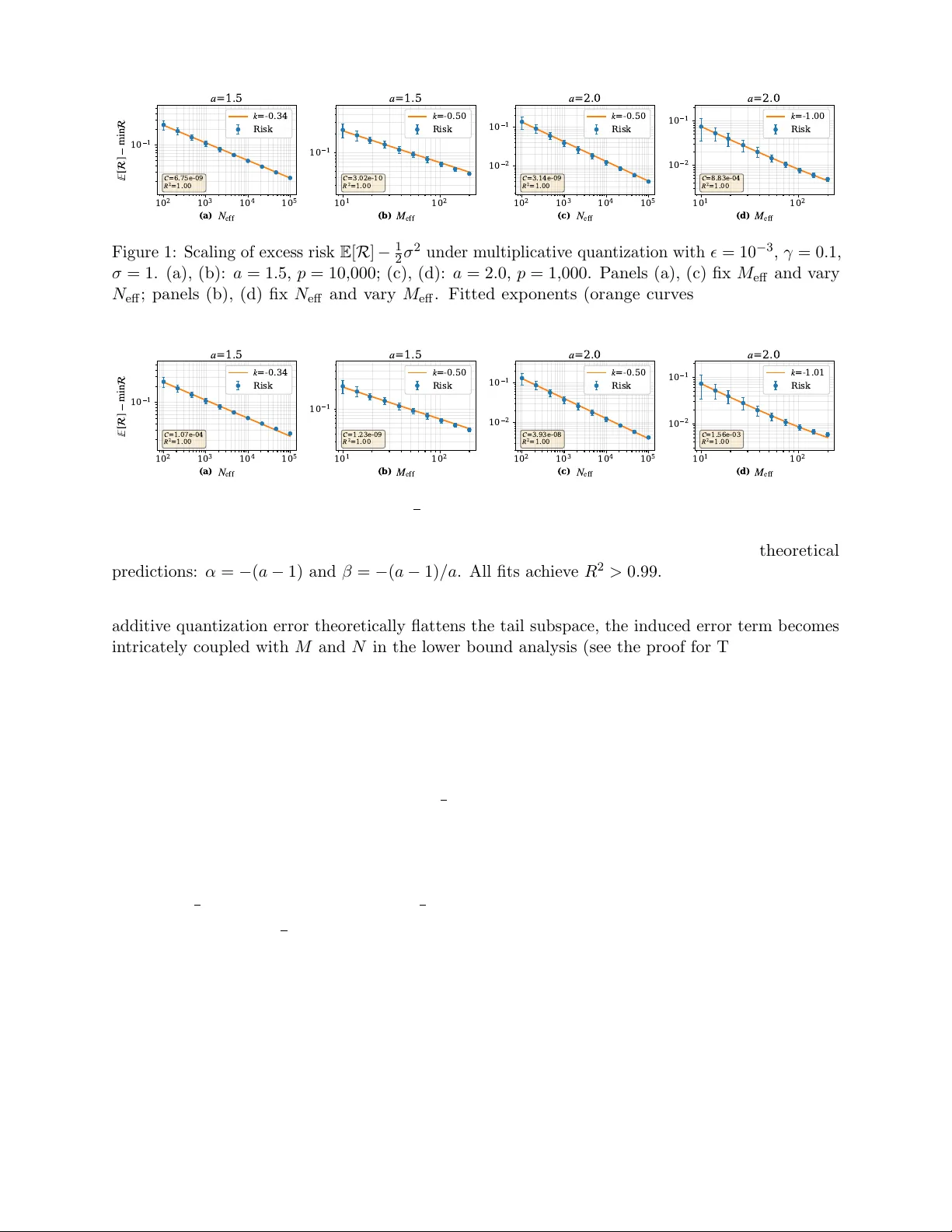
Scaling La ws for Precision in High-Dimensional Linear Regression Dec hen Zhang ∗ Xuan T ang † Yingyu Liang ‡ Difan Zou § F ebruary 27, 2026 Abstract Lo w-precision training is critical for optimizing the trade-oﬀ betw een mo del qualit y and training costs, necessitating the join t allo cation of mo del size, dataset size, and numerical precision. While empirical scaling la ws suggest that quan tization impacts eﬀectiv e mo del and data capacities or acts as an additiv e error, the theoretical mechanisms go v erning these eﬀects remain largely unexplored. In this w ork, w e initiate a theoretical study of scaling laws for lo w-precision training within a high-dimensional sketc hed linear regression framework. By analyzing multiplicativ e (signal-dependent) and additiv e (signal-indep endent) quan tization, we iden tify a critical dichotom y in their scaling b ehaviors. Our analysis reveals that while b oth sc hemes in tro duce an additiv e error and degrade the eﬀectiv e data size, they exhibit distinct eﬀects on eﬀectiv e model size: multiplicativ e quantization maintains the full-precision model size, whereas additive quan tization reduces the eﬀective model size. Numerical exp eriments v alidate our theoretical ﬁndings. By rigorously characterizing the complex interpla y among mo del scale, dataset size, and quan tization error, our work pro vides a principled theoretical basis for optimizing training proto cols under practical hardw are constraints. 1 In tro duction The remark able success of large language mo dels (LLMs) has b een largely driven b y the scaling of model parameters and training datasets, gov erned b y the no w-canonical neural scaling la ws ( Kaplan et al. , 2020 ; Hoﬀmann et al. , 2022 ). How ev er, the prohibitiv e computational and memory costs asso ciated with such scaling ha ve made lo w-precision training indisp ensable ( Courbariaux et al. , 2014 ; W ang et al. , 2018 ; Sun et al. , 2020 ; Hao et al. , 2025 ). State-of-the-art framew orks no w extensively lev erage mixed- or lo w-precision formats for gradien ts, w eights, and optimizer states ( P eng et al. , 2023 ; W ortsman et al. , 2023 ; Xi et al. , 2024 ; Fishman et al. , 2024 ; Liu et al. , 2024 ), sho wing that aggressively low-precision training can scale to trillion-token w orkloads without compromising accuracy . This shift fundamentally alters the scaling landscap e, in tro ducing a complex in terplay b etw een mo del size, dataset size, and numerical precision. Optimizing the performance of LLMs th us necessitates a rigorous understanding to guide the join t allocation of ﬁxed compute or memory budgets across these three dimensions. Despite the practical urgency , our understanding of low-precision scaling remains predominantly empirical. Recen t studies ha ve prop osed diﬀeren t functional forms to describ e how bit-width ∗ Institute of Data Science, The Univ ersity of Hong Kong. Email: dechenzhang @connect.hku.hk † Sc ho ol of Computing & Data Science, The Universit y of Hong Kong. Email: xuantang8 @connect.hku.hk ‡ Institute of Data Science and School of Computing & Data Science, The Universit y of Hong Kong. Email: yingyul @hku.hk § Sc ho ol of Computing & Data Science and Institute of Data Science, The Universit y of Hong Kong. Email: dzou @hku.hk 1 aﬀects the scaling b ehavior in lo w-precision training ( Kumar et al. , 2024 ; Sun et al. , 2025 ). One line of research p osits that quantization eﬀectiv ely reduces the mo del’s capacity: L ( M , N , Q ) ≈ AM eﬀ ( M , Q ) − α + B N − β + E , where M eﬀ represen ts an eﬀectiv e model size reduced by quan tization op erations ( Kumar et al. , 2024 ). While others formulate quantization as an additiv e error term: L ( M , N , Q ) ≈ AM − α + B N − β + E + δ ( M , N , Q ), where δ acts as an explicit p enalty term dep endent on quantization ( Sun et al. , 2025 ). Crucially , these are purely empirical ﬁts and there exists no uniﬁed theoretical framework to determine whic h form ulation, eﬀectiv e size reduction or additiv e error, is ph ysically correct, nor to mechanistically account for the intricate eﬀects of speciﬁc training algorithms and mixed-precision strategies. Recen t studies on the theoretical understanding of scaling laws hav e focused on analyzing the exact training dynamics of SGD using linear mo dels ( Lin e t al. , 2024 , 2025 ; Li et al. , 2025 ; Y an et al. , 2025 ). In particular, Lin et al. ( 2024 ) resolved the discrepancy b etw een neural scaling laws and traditional statistical learning theory by adopting an inﬁnite-dimensional sk etc hed linear regression framew ork with p o wer-la w sp ectra. Building on this, Lin et al. ( 2025 ) and Y an et al. ( 2025 ) extended one-pass SGD to m ulti-pass SGD, showing the b eneﬁt of increasing the multi-epo c h coun t K . In a parallel av en ue of research, Li et al. ( 2025 ) c haracterized ho w the learning rate sc hedule shapes scaling b eha viors. These works ha v e rep eatedly demonstrated that such high-dimensional linear setups, despite their simplicit y , can faithfully capture key phenomenological asp ects of deep learning. Motiv ated b y these successes, we initiate the theoretical study of scaling la ws for lo w-precision training within a high-dimensional sk etched linear regression setup. Our setting. W e assume access to M -dimensional sk etc hed co v ariates and their resp onses, that is, ( Sx , y ), where S ∈ R M × H is a ﬁxed sketc h matrix, x ∈ H ⊂ R p is the data vector and H is a Hilb ert space that is either ﬁnite-dimensional or coun tably inﬁnite-dimensional. W e focus on the Gaussian sketc h matrix ( Lin et al. , 2024 , 2025 ; Chen et al. , 2025b ; Ding et al. , 2025 ). That is, en tries of S are independently sampled from N (0 , 1 / M ). W e then consider linear mo del with M trainable parameters given by: f v : H → R , x → ⟨ v , Sx ⟩ , where v ∈ R M are the trainable parameters. Our goal is to b ound the p opulation risk R M ( v ) := 1 2 E [( ⟨ Sx , v ⟩ − y ) 2 ] , v ∈ R M , where the exp ectation is conditioned on the sk etc h matrix S 1 . W e consider training f v via constan t- stepsize one-pass quan tized sto c hastic gradient descent (SGD) ( Zhang et al. , 2025 ). The parameter v t is updated as follo ws: v t = v t − 1 + γ g ( q ) f ( q ) , t = 1 , ..., N , (quan tized SGD) f ( q ) = Q f ( Q s ( S ) Q d ( x t )) , g ( q ) = Q o ( Q l ( y t ) − Q a ( Q f ( Q s ( S ) Q d ( x t )) ⊤ Q p ( v t − 1 ))) , where ( x t , y t ) N t =1 are indep endent samples and γ is the stepsize, and Q d , Q s , Q f , Q l , Q p , Q a , Q o are indep endent general quantization op erations for data, sk etc h matrix, feature, lab els, model parameters, activ ations and output gradients resp ectively , and f ( q ) is the quan tized feature and g ( q ) is the quantized output gradient. Without loss of generality , we assume the initial parameter is v 0 = 0. The output of the SGD algorithm is the the iterate a v erage v N := 1 N P N − 1 t =0 v t . 1 In this pap er, all exp ectations are conditioned on S . 2 Notations. F or tw o p ositiv e-v alued functions f ( x ) and g ( x ), w e write f ( x ) ≲ g ( x ) or f ( x ) ≳ g ( x ) if f ( x ) ≤ cg ( x ) or f ( x ) ≥ cg ( x ) holds for some absolute (if not otherwise sp eciﬁed) constan t c > 0 resp ectiv ely . W e write f ( x ) ≂ g ( x ) if f ( x ) ≲ g ( x ) ≲ f ( x ). F or t wo v ectors u and v in a Hilb ert space, w e denote their inner pro duct b y ⟨ u , v ⟩ or u ⊤ v . F or t wo matrices A and B of appropriate dimensions, we deﬁne their inner pro duct b y ⟨ A , B ⟩ := tr  A ⊤ B  . W e use ∥ · ∥ to denote the operator norm for matrices. F or a positive semi-deﬁnite (PSD) matrix A and a v ector v of appropriate dimension, w e write ∥ v ∥ 2 A = v ⊤ Av . Our main results. Assuming that the sp ectrum of the data cov ariance matrix satisﬁes a p ow er-la w of degree a > 1, w e analyze scaling la ws under tw o standard quantization schemes: multiplicativ e quan tization (where error v ariance scales with signal magnitude) and additive quantization (where error v ariance is independent of the signal). Informally , the population risk upper b ound for b oth sc hemes can be uniﬁed as: R M ( v N ) ≲ R ∗ + 1 M eﬀ ( M , ϵ ) a − 1 + 1 N eﬀ ( N , ϵ ) a − 1 a + δ ( ϵ ) , where M is the mo del size, N is the data size and R ∗ represen ts a p ositiv e irreducible risk, ϵ generically represents the quan tization error (which v anishes in full-precision training) and δ ( ϵ ) denotes an additive err or induced b y ϵ . The k ey quantities M eﬀ and N eﬀ represen t the eﬀe ctive mo del size and eﬀe ctive data size , resp ectiv ely . W e demonstrate a critical div ergence in how the tw o quan tization sc hemes aﬀect these quan tities. • Eﬀectiv e Data Size ( N eﬀ ): Both sc hemes reduce the eﬀectiv e data size via noise-ampliﬁcation quan tization error ϵ noise and spectral-distortion quantization error ϵ spect . • Eﬀectiv e Mo del Size ( M eﬀ ): Multiplicative quan tization (FP-lik e) preserv es the full mo del capacit y (i.e., M eﬀ ≈ M ), whereas additiv e quan tization (INT-like) strictly contracts it driven by noise ampliﬁcation and sp ectral distortion factors analogous to those reducing N eﬀ . W e refer to Theorem 4.1 and Theorem 4.2 for formal statements of upp er b ounds. This theoretical dic hotomy provides a rigorous basis for recent empirical ﬁndings in lo w-precision training. Speciﬁcally , our additive quantization scaling law captures the eﬀectiv e mo del shrink age observed in in teger quan tization ( Kumar et al. , 2024 ), while our m ultiplicative quantization scaling la w corroborates the observ ation that ﬂoating-p oint quan tization preserves eﬀectiv e mo del capacity ( Sun et al. , 2025 ). Complemen ting the upp er b ounds, w e establish the ﬁrst p opulation risk lo w er b ounds for lo w-precision training (see Theorem 4.3 and Theorem 4.4 for details). These low er b ounds v alidate the existence of the additive error and the reduction of eﬀective data size, conﬁrming that these mec hanisms are fundamen tal in lo w-precision training. 2 Related W ork Empirical scaling laws for quantized training. Recen t researc h has fo cused on empirically c haracterizing the scaling behaviors of quantized training ( Dettmers and Z ettlemo yer , 2023 ; Ouyang et al. , 2024 ; Kumar et al. , 2024 ; T ao et al. , 2024 ; F rantar et al. , 2025 ; Chen et al. , 2025a ; Sun et al. , 2025 ; Liu et al. , 2025 ). One line of w ork conceptualizes quan tization as a mec hanism that eﬀectiv ely reduces mo del size ( Kumar et al. , 2024 ; F rantar et al. , 2025 ). Notably , Kumar et al. ( 2024 ) prop osed uniﬁed scaling la ws under integer quan tization co v ering low-precision training, quantization-a w are training (QA T), and post-training quantization (PTQ). F or lo w-precision training, they mo deled the loss as L ( M , N , P ) ≈ AM eﬀ ( M , P ) − α + B N − β + E , where M eﬀ ( M , P ) ≈ M (1 − e − P /γ ) represen ts 3 the eﬀective mo del capacity contracted by low precision. Another stream of research mo dels quan tization as an additive error ( Chen et al. , 2025a ; Sun et al. , 2025 ). Sun et al. ( 2025 ) established scaling la ws for low-precision training under ﬂoating-p oint (FP) formats, formulating the loss with a precision-dep endent error term: L ( M , N , P ) ≈ AM − α + B N − β + E + δ ( M , N , P ). They sho wed that quantization induces a predictable deviation from the standard p ow er law. In a parallel eﬀort targeting integer QA T, Chen et al. ( 2025a ) extended this framework to accoun t for quan tization gran ularit y ( G ), modeling the loss via a similar additiv e penalty: L ( M , N , P ) ≈ AM − α + B N − β + E + δ ( M , N , P , G ). High-dimensional linear regression via SGD. Theoretical guarantees for generalization ha ve garnered signiﬁcant atten tion in machine learning. Seminal work by Bartlett et al. ( 2020 ); Tsigler and Bartlett ( 2023 ) established nearly tigh t upp er and low er excess risk b ounds for linear (ridge) regression under general regularization schemes. In the classical under-parameterized regime, extensiv e literature has explored the learnabilit y of iterate-av eraged SGD ( Poly ak and Juditsky , 1992 ; Bac h and Moulines , 2013 ; D´ efossez and Bac h , 2015 ; Dieulev eut et al. , 2017 ; Jain et al. , 2017 , 2018 ). Conv ersely , in the mo dern ov erparameterized setting, one-pass SGD has b een rigorously studied ( Dieulev eut and Bach , 2015 ; Berthier et al. , 2020 ; V arre et al. , 2021 ; Zou et al. , 2021 ; W u et al. , 2022a , b ; Zhang et al. , 2024 ), yielding framew orks to c haracterize how optimization dynamics inﬂuence generalization across v arious data distributions. Additionally , another line of work has analyzed multi-pass SGD for high-dimensional ℓ 2 -regularized least squares, detailing excess risk b ounds ( Lei et al. , 2021 ; Zou et al. , 2022 ) and exact risk dynamics ( Paquette et al. , 2024a ). More recen tly , Zhang et al. ( 2025 ) established the ﬁrst excess risk upp er b ounds for lo w-precision training, c haracterizing the impact of quantization on the learning dynamics of SGD in linear regression. Our w ork builds up on this foundation b y extending their theoretical framew ork to sketc hed linear regression. F urthermore, we provide a critical missing piece b y deriving the ﬁrst excess risk lo wer b ounds for low-precision training. Theoretical understandings of scaling la ws. Several recen t studies hav e sough t to formalize and explain empirical scaling la ws using conceptually simpliﬁed linear mo dels ( Bahri et al. , 2024 ; A tanasov et al. , 2024 ; Paquette et al. , 2024b ; Bordelon et al. , 2024 ; Lin et al. , 2024 , 2025 ; Y an et al. , 2025 ; Li et al. , 2025 ; Ding et al. , 2025 ). Early theoretical attempts fo cused on asymptotic regimes: Bahri et al. ( 2024 ) analyzed a linear teac her-studen t mo del with p ow er-la w sp ectra, sho wing that the test loss of the ordinary least squares (OLS) estimator decays as a p o wer law in sample size N (or model size M ) when the other dimension approaches inﬁnity . Similarly , Bordelon et al. ( 2024 ) studied gradien t ﬂo w in linear random feature mo dels, establishing p ow er-law scaling with respect to one of N , M , or training time T , pro vided the other parameters remain eﬀectively inﬁnite. A piv otal step tow ards realistic ﬁnite-sample analysis is made by Lin et al. ( 2024 ). Building on analysis tec hniques from Zou et al. ( 2021 ) and W u et al. ( 2022a ), they analyzed the last iterate of one-pass SGD in a sketc hed linear mo del and presen ted the ﬁrst systematic deriv ation of a ﬁnite-sample join t scaling la w (in both M and N ) that aligns with empirical observ ations ( Kaplan et al. , 2020 ). Subsequen t researc h expands this framew ork to more complex settings. Lin et al. ( 2025 ) extended the analysis to data reuse (m ulti-pass SGD), sho wing that for relativ ely small multi-epo ch count K , ev ery new ep o ch leads to a linear gain in eﬀective sample size, i.e., N eﬀ ≂ N K . Building on this, Y an et al. ( 2025 ) provided a ﬁner-grained c haracterization for strongly conv ex or Zipf-distributed data. They demonstrated that for large m ulti-ep o c h count K , the eﬀectiv e reuse rate N eﬀ / N plateaus at a problem-dep endent v alue that gro ws with N . More recently , Li et al. ( 2025 ) established functional scaling la ws and analyzed how learning rate sc hedules shap e these scaling b ehaviors. 4 3 Theoretical Setup 3.1 Quan tization Op eration F or all quan tization op erations in ( quan tized SGD ), w e emplo y the sto c hastic quantization metho d ( Mark ov et al. , 2023 ; Mo doranu et al. , 2024 ; Ozk ara et al. , 2025 ), whic h un biasedly rounds v alues using randomly adjusted probabilities. W e summarize this in the follo wing assumption. Assumption 3.1. L et Q i , i ∈ { d, s, f , l, p, a, o } b e the c o or dinate-wise quantization op er ation for data, sketch matrix, fe atur e, lab el, mo del p ar ameters, activations, and output gr adients, r esp e ctively. Then for any u , the quantization op er ation is unbiase d: E [ Q i ( u ) | u ] = u . F urthermore, to b etter unco ver the eﬀect of quantization, we consider the following tw o types of quan tization error: multiplicativ e quantization and additive quantization, which are motiv ated by abstracting the b ehavior of prev alen t n umerical formats used in practice ( Zhang et al. , 2025 ). Deﬁnition 3.1. L et Q b e an unbiase d quantization op er ation. We formalize two pr actic al quantiza- tion schemes: • Multiplic ative quantization. We c al l the quantization to x is ( ϵ, ϵ )-multiplic ative if the c onditional se c ond moment of quantization err or is pr op ortional to the outer pr o duct of r aw data itself, i.e., ϵ xx ⊤ ⪯ E [( Q ( x ) − x ) ( Q ( x ) − x ) ⊤ | x ] ⪯ ϵ xx ⊤ . F or multiplic ative quantization to matrix X , we extend the deﬁnition to ϵ XAX ⊤ ⪯ E [( Q ( X ) − X ) A ( Q ( X ) − X ) ⊤ | X ] ⪯ ϵ XAX ⊤ , for any PSD matrix A . • A dditive quantization. We c al l the quantization to x is ( ϵ, ϵ )-additive if the c onditional se c ond moment of quantization err or is pr op ortional to identity, i.e., ϵ I ⪯ E [( Q ( x ) − x ) ( Q ( x ) − x ) ⊤ | x ] ⪯ ϵ I , for any PSD matrix A . F or additive quantization to matrix X , we extend the deﬁnition to ϵ tr( A ) I ⪯ E [( Q ( X ) − X ) A ( Q ( X ) − X ) ⊤ | X ] ⪯ ϵ tr( A ) I , for any PSD matrix A . This theoretical distinction is grounded in practical quan tization sc hemes. F or instance, in teger quan tization (e.g., INT8, INT16) uses a ﬁxed bin length, resulting in an error that is largely indep enden t of the v alue’s magnitude ( W u et al. , 2020 ). This characteristic aligns with our deﬁnition of additive quantization, where the error v ariance is uniform across co ordinates. Conv ersely , ﬂoating- p oin t quan tization (e.g., FP8, FP32) employs a v alue-a w are bin length via its exp onen t and mantissa bits (e.g., E4M3 format in FP8) ( Kuzmin et al. , 2022 ). This structure causes the quantization error to scale with the magnitude of the v alue itself, corresp onding to m ultiplicative quantization. 3.2 Data Mo del W e then state the regularit y assumptions on the data distribution, which align with those common in prior works ( Zou et al. , 2021 ; W u et al. , 2022a , b , 2023 ). As lo w-precision training is p erformed on quan tized feature ˜ x ( q ) = Q f ( Q s ( S ) Q d ( x )) , w e formulate these assumptions on the lo w-precision feature format following Zhang et al. ( 2025 ). 5 Assumption 3.2 (Data cov ariance) . L et H := E [ xx ⊤ ] b e the data c ovarianc e and H ( q ) f := E [ ˜ x ( q ) ( ˜ x ( q ) ) ⊤ ] b e the quantize d fe atur e c ovarianc e. Assume that tr ( H ) , tr ( H q f ) and al l entries of H , H ( q ) f ar e ﬁnite. F or c onvenienc e, we assume that H is strictly p ositive deﬁnite. Let H = P i λ i v i v ⊤ i b e the eigen-decomp osition of H , where { λ i } ∞ i =1 are the eigenv alues of H sorted in non-increasing order and v i are the corresp onding eigenv ectors. W e denote H 0: k := P k i =1 λ i v i v ⊤ i , H k : ∞ := P i>k λ i v i v ⊤ i , I 0: k := P k i =1 v i v ⊤ i , I k : ∞ := P i>k v i v ⊤ i . Similarly , we denote the eigen-decomposition of H ( q ) f as H ( q ) f = P i ˜ λ ( q ) i v ( q ) i v ( q ) i ⊤ and correspondingly obtain H ( q ) f , 0: k , H ( q ) f ,k : ∞ , I ( q ) f , 0: k , I ( q ) f ,k : ∞ , where { ˜ λ ( q ) i } ∞ i =1 are the eigen v alues of H ( q ) f . In line with Zhang et al. ( 2025 ), w e extend the fourth momen t and noise assumptions ( Zou et al. , 2021 ; W u et al. , 2022b , a , 2023 ) to quantized features. Assumption 3.3 (F ourth-momen t conditions) . Assume that the fourth moment of ˜ x ( q ) is ﬁnite and ther e exist c onstants α, β > 0 such that for any PSD matrix A , H ( q ) f AH ( q ) f + β tr( H ( q ) f A ) H ( q ) f ⪯ E h ˜ x ( q ) ( ˜ x ( q ) ) ⊤ A ˜ x ( q ) ( ˜ x ( q ) ) ⊤ i ⪯ α tr( H ( q ) f A ) H ( q ) f . Regarding the noise assumptions, we ﬁrst deﬁne the p opulation risk and global optimum in quan tized feature space: R ( q ) M ( v ) := 1 2 E [( ⟨ ˜ x ( q ) , v ⟩ − Q l ( y )) 2 ] , v ∈ R M , with global optimum v ( q ) ∗ := argmin v R ( q ) M ( v ). Assumption 3.4 (Noise conditions) . Denote ξ := Q l ( y ) − ⟨ v ( q ) ∗ , ˜ x ( q ) ⟩ . Assume ther e exists a p ositive c onstants σ , σ > 0 such that σ 2 H ( q ) f ⪯ E [ ξ 2 ˜ x ( q ) ( ˜ x ( q ) ) ⊤ ] ⪯ σ 2 H ( q ) f . A k ey distinction from the assumptions in Zhang et al. ( 2025 ) is that w e require lo wer b ounds on the noise and fourth moment to establish b oth upp er and low er risk b ounds. W e would like to remark that under the fourth moment assumption and noise assumption on the full-precision data, Assumption 3.3 and 3.4 can b e v eriﬁed under speciﬁc multiplicativ e quantization and additiv e quan tization sc hemes. W e defer the veriﬁcation in Section H . T o simplify the scaling-law b eha vior, we assume sp eciﬁc data distribution where the data sp ectrum satisﬁes a pow er law and the optimal parameter satisﬁes a prior ( Lin et al. , 2024 ). Sp eciﬁcally , we consider the population risk for w ∈ H : R ( w ) := 1 2 E [( ⟨ x , w ⟩ − y ) 2 ] , w ∈ H , with global optimum w ∗ := argmin w R ( w ). Assumption 3.5 (Distributional conditions) . We assume the wel l-sp e ciﬁe d mo del, i.e., E [ y | x ] = x ⊤ w ∗ and σ 2 := E  ( y − x ⊤ w ∗ ) 2  , and the p ar ameter prior, i.e., E [ w ∗ w ∗ ⊤ ] = I . We also assume the data sp e ctrum is p olynomial, i.e., ther e exists a > 1 such that the eigenvalues of H satisfy λ i ≂ i − a , i > 0 . 4 Main Theory In this section, w e demonstrate lo w-precision training scaling la ws when the data sp ectrum satisﬁes a p o wer law. W e state the scaling laws for multiplicativ e quan tization and additiv e quan tization resp ectiv ely . 6 4.1 Multiplicativ e Quan tization In this section, w e consider for an y i ∈ { s, d, f , p, a, o } , there exist ϵ i suc h that quantization Q i is ϵ i -m ultiplicative 2 . Motiv ated by the insigh t from Zhang et al. ( 2025 ) that diﬀeren t quan tization targets exert distinct inﬂuences on the risk, w e ﬁrst deﬁne a set of compound quan tization co eﬃcients to aggregate individual quan tization errors based on their distinct ph ysical eﬀects on the learning dynamics. This form ulation streamlines the presen tation and elucidates the structural impact of quan tization. Firstly , to capture the distortion to feature sp ectrum and the gap b et ween quantized feature space and full-precision data space, we deﬁne ϵ ( M ) 3 = 1 − 1 (1 + ϵ d )(1 + ϵ f )(1 + ϵ s ) , whic h arises from feature, sk etch and data quantization. Secondly , to characterize the noise ampliﬁcation during training, we deﬁne ϵ ( M ) 2 = (1 + ϵ o ) (1 + ϵ p + (1 + ϵ p ) ϵ a ) − 1 , whic h arises from parameter, activ ation and output gradient quantization. Generally , the comp ound co eﬃcien ts ϵ ( M ) 3 and ϵ ( M ) 2 scale monotonically with the underlying quantization sev erity . In standard training regimes where the individual quan tization errors (e.g., ϵ o , ϵ p , ϵ d ) are small ( < 1), these co eﬃcien ts remain small quantities of comparable magnitude. In particular, ϵ ( M ) 3 is strictly less than 1. Notably , they v anish strictly to zero in the full-precision limit. With these notations, we are no w ready to state the main scaling laws under multiplicativ e quan tization. Theorem 4.1 (Scaling law under m ultiplicativ e quantization, an upp er b ound) . Supp ose γ < 1 (1+ ϵ ( M ) 2 ) α tr( H ( q ) f ) . F or any i ∈ { s, d, f , p, a, o } , if ther e exist ϵ i such that quantization Q i is ϵ i - multiplic ative, then under Assumption 3.1 , 3.2 , 3.3 , 3.4 and 3.5 , if H ( q ) f and SHS ⊤ c ommute, with pr ob ability at le ast 1 − e − Ω( M ) over the r andomness of S , E R M ( v N ) ≲ 1 M a − 1 eﬀ + 1 N ( a − 1) /a eﬀ + σ 2 + ϵ ( M ) 3 , (1) wher e M eﬀ = M and N eﬀ = N  1+ ϵ ( M ) 2 (1 − ϵ ( M ) 3 ) 1 a  − a/ ( a − 1) . Theorem 4.1 rigorously quantiﬁes the dual impact of m ultiplicative quantization: the reduction of eﬀective data size and the introduction of an additiv e error. Sp eciﬁcally , the reduction in eﬀective data size N eﬀ stems from tw o mec hanisms: the ampliﬁcation of optimization noise due to quantized parameters, gradients and activ ations (captured b y ϵ ( M ) 2 ), and the distortion of the feature sp ectrum (captured b y ϵ ( M ) 3 ). Meanwhile, the additiv e error term arises from the gap betw een the quantized feature space and the full-precision data space (captured b y ϵ ( M ) 3 ). These mechanisms align with the ﬁndings of how quan tization aﬀects learnabilit y in Zhang et al. ( 2025 ). Notably , in the absence of quan tization ( ϵ ( M ) i = 0), Theorem 4.1 recov ers the classical full-precision scaling la w established in Lin et al. ( 2024 ). A critical insight from Theorem 4.1 is that m ultiplicativ e quan tization does not reduce the eﬀectiv e mo del size, whic h aligns with some empirical studies ( Chen et al. , 2025a ; Sun et al. , 2025 ). In tuitively , this inv ariance arises from the signal-dependent nature of m ultiplicative quan tization, 2 This means we only access to the upp er b ound of quantization errors deﬁned in Deﬁnition 3.1 . 7 whic h preserv es the sp ectral structure of the quantized feature co v ariance. Sp eciﬁcally , since the quan tization error scales with the signal magnitude, it deca ys alongside the signal in the high- dimensional tail subspace. This ensures that the tail subspace of quantized feature sp ectrum deca ys as that of the full-precision sp ectrum (up to a constant scalar), thereby preserving the learnabilit y of eac h parameter. Consequen tly , m ultiplicative quantization maintains M eﬀ = M . Our Theorem 4.1 assumes commutativit y b etw een the quantized feature co v ariance H ( q ) f and the sk etched cov ariance SHS ⊤ to deriv e a sharper b ound. W e would also like to remark that, without this comm utativ e condition, the quan tization error ma y pro ject non-trivially on to sensitive eigen-directions. While an upp er b ound can still b e deriv ed in general case (see Theorem C.3 for details), this misalignment introduces an additional p enalty related to the condition n um b er of SHS ⊤ . T o isolate the fundamental scaling b ehavior, we apply the commutativit y assumption here. 4.2 Additiv e Quan tization In this section, we consider for an y i ∈ { s, d, f , p, a, o } , there exist ϵ i suc h that quan tization Q i is ϵ i -additiv e. Analogous to the m ultiplicativ e case, we deﬁne a set of comp ound quan tization co eﬃcien ts to streamline the presen tation. Regarding the discrepancy b etw een the quan tized feature co v ariance and the original data co v ariance, we deﬁne: ϵ ( A ) 3 = ϵ f + ϵ s (1 + ϵ d p ) + ϵ d p M M − a +  ϵ f + ϵ s (1 + ϵ d p ) + ϵ d p M  . Regarding the noise ampliﬁcation, w e deﬁne ϵ ( A ) 2 = ϵ a + ϵ o + ϵ p [1 + pϵ d + M ( ϵ f + ϵ s + ϵ s ϵ d p )] . Similar to the m ultiplicative case, these co eﬃcients are small quan tities that scale monotonically with the quantization sev erity and v anish strictly in the full-precision limit. How ev er, we note that, unlik e m ultiplicative co eﬃcients which are largely dimension-indep endent, ϵ ( A ) 2 and ϵ ( A ) 3 scale with the data dimension p and mo del size M . This distinction arises b ecause additiv e quantization in tro duces constant quantization v ariance that is indep endent across all co ordinates. Moreov er, since the additive quantization error constitutes a ﬁxed ﬂo or rather than scaling with the signal, ϵ ( A ) 3 m ust explicitly accoun t for its magnitude relativ e to the minim um eigenv alues of the data sp ectrum ( M − a ). With these notations, w e no w present the main scaling la ws for lo w-precision training under additiv e quan tization. Theorem 4.2 (Scaling law under additiv e quan tization, an upp er b ound) . Supp ose γ < 1 α tr( H ( q ) f ) . F or any i ∈ { s, d, f , p, a, o } , if ther e exist ϵ i such that quantization Q i is ϵ i -additive, then under Assumption 3.1 , 3.2 , 3.3 , 3.4 and 3.5 , if H ( q ) f and SHS ⊤ c ommute, with pr ob ability at le ast 1 − e − Ω( M ) over the r andomness of S , E R M ( v N ) ≲ 1 M a − 1 eﬀ + 1 N ( a − 1) /a eﬀ + σ 2 + ϵ ( A ) 3 , (2) wher e N eﬀ = N  1+ ϵ ( A ) 2 (1 − ϵ ( A ) 3 ) 1 /a  − a a − 1 , and crucial ly, M eﬀ = M " 1 + (1 + ϵ ( A ) 2 ) ( ϵ ( A ) 3 ) 2 1 − ϵ ( A ) 3 # − 1 / ( a − 1) . 8 Theorem 4.2 c haracterizes a fundamen tal dichotom y b et ween additive and m ultiplicativ e quanti- zation. Unlike the m ultiplicative case, additiv e quan tization not only introduces an additiv e error ﬂo or and reduces the eﬀectiv e data size, but also reduces the eﬀective mo del size. The interpretation is that additiv e quan tization injects an constan t lev el quan tization error across the entire spectrum of the quan tized feature co v ariance H ( q ) f . Consequently , this constan t error o v erwhelms the in trinsic signal in the sp ectral tail and results in a ﬂattened sp ectrum, rendering the tail dimensions useless for learning. Hence, the mo del cannot eﬀectively leverage its full parameter count, leading to a reduction in M eﬀ . Our analysis further reveals that the degradation of eﬀectiv e mo del size ( M eﬀ ) and eﬀective data size ( N eﬀ ) is go v erned by similar physical mechanisms. As derived in Theorem 4.2 , b oth eﬀectiv e data size and eﬀectiv e mo del size are modulated b y the same noise ampliﬁcation factor ϵ ( A ) 2 and spectral distortion factor ϵ ( A ) 3 . This mec hanisms align with Theorem 4.1 under multiplicativ e quan tization and prior work ( Zhang et al. , 2025 ). Similar to multiplicativ e case, under full precision, Theorem 4.2 reco vers the result in Lin et al. ( 2024 ) and the commutativit y condition is assumed here to isolate the fundamental scaling behavior. A general bound relaxing this assumption is in Theorem C.4 . Connection with empirical scaling la ws for low-precision training. Our theoretical dis- tinction b etw een additive and m ultiplicativ e quantization pro vides a mec hanistic explanation for the div ergent empirical behaviors observ ed in in teger v ersus ﬂoating-p oint training. Firstly , the empirical observ ation in Kumar et al. ( 2024 ) that in teger quan tization eﬀectively reduces mo del capacity aligns with our additive quantization (INT-like) scaling la w (Theorem 4.2 ). Our theory further rev eals the mechanism: a constan t lev el quan tization error ﬂattens the tail subspace, eﬀectively rendering those dimensions uninformativ e and leading to the theoretically derived reduction in M eﬀ . In con trast, Sun et al. ( 2025 ) found that ﬂoating-p oint quantization primarily introduces an additive loss term rather than shrinking the mo del size. This corrob orates our multiplicativ e quan tization (FP-lik e) scaling law (Theorem 4.1 ), which establishes that the eﬀective mo del size remains in v arian t ( M eﬀ = M ). The underlying mechanism is that multiplicativ e quantization preserves the relativ e sp ectral structure, ensuring the quantization error in the tail subspace scales do wn with the signal. 4.3 Lo w er Bound Analysis T o tighten our analysis, w e establish scaling la w lo w er b ounds under m ultiplicative and additiv e quan tization. In low er b ound analysis, w e consider lo w-precision w ell-sp eciﬁc mo del: E  ξ | ˜ x ( q )  = 0, whic h is extended from the standard full-precision well-speciﬁc mo del assumption ( Zou et al. , 2021 ; W u et al. , 2022a , b ). 4.3.1 Multiplicativ e Quan tization W e extend the comp ound co eﬃcien ts deﬁned in Section 4.1 to their lo w er-b ound counterparts. The deﬁnitions utilize the minim um quan tization errors ϵ . F or simplicit y , w e provide explicit deﬁnitions for ϵ ( M ) 2 , ϵ ( M ) 3 in Section E.1 . Theorem 4.3 (Scaling la w under m ultiplicative quan tization, a lo w er b ound) . Supp ose γ < 1 / ˜ λ ( q ) 1 . F or i ∈ { d, f , s, p, a, o } , if ther e exist c onstants ( ϵ i , ϵ i ) such that Q i is ( ϵ i , ϵ i ) -multiplic ative, then under Assumption 3.1 , 3.2 , 3.3 , 3.4 and 3.5 , for suﬃciently lar ge N > 500 , if H ( q ) f and SHS ⊤ ar e 9 c ommutative, with pr ob ability at le ast 1 − e − Ω( M ) over the r andomness of S , it holds E R M ( v N ) ≳ 1 M a − 1 eﬀ + 1 N ( a − 1) /a eﬀ + σ 2 +  ϵ ( M ) 3  2 + ϵ ( M ) 3 N  1 − ϵ ( M ) 3  , (3) wher e M eﬀ = M and N eﬀ = N  (1 − ϵ ( M ) 3 )(1+ ϵ ( M ) 2 ) (1 − ϵ ( M ) 3 ) 1 a  − a a − 1 . Theorem 4.3 matches the form of scaling la w deriv ed in the upp er bound: m ultiplicative quan tization inheren tly reduces the eﬀectiv e data size N eﬀ via noise ampliﬁcation ( ϵ ( M ) 2 ) and sp ectral distortion ( ϵ ( M ) 3 ), while introducing an una voidable additiv e error via the gap b etw een quan tized feature space and full-precision data space ( ϵ ( M ) 3 ). Generally , the low er b ound for the eﬀectiv e data size N eﬀ in Theorem 4.3 do es not strictly matc h the upper b ound. This discrepancy stems from the gap b et ween the worst-case ( ϵ ) and b est-case ( ϵ ) quan tization errors. Matc hing b ounds are achiev ed in the sharp quantization limit where ϵ ≈ ϵ 3 . W e note that this clean scaling law form holds in tw o asymptotic regimes where the interpla y b et ween M and N is w ell-separated, eﬀectiv ely rendering the ratio term N / M of strict higher order. See Theorem E.2 for the explicit deﬁnition of these regimes. F or completeness, a general p opulation risk lo w er b ound co vering the full space of ( M , N ) is pro vided in Theorem D.3 in the Appendix. 4.3.2 Additiv e Quan tization Analogous to the multiplicativ e case, we establish the low er b ound for additiv e quantization by extending the compound co eﬃcients to their low er-b ound coun terparts. F or simplicity , w e defer the deﬁnitions of ϵ ( A ) 2 , ϵ ( A ) 3 to Section E.2 . Theorem 4.4 (Scaling la w under additiv e quan tization, a lo wer b ound) . Supp ose γ < 1 ˜ λ ( q ) 1 . F or i ∈ { d, f , s, p, a, o } , if ther e exist c onstants ( ϵ i , ϵ i ) such that Q i is ( ϵ i , ϵ i ) -additive, then under Assumption 3.1 , 3.2 , 3.3 , 3.4 and 3.5 , for suﬃciently lar ge N > 500 , if H ( q ) f and SHS ⊤ ar e c ommutative, with pr ob ability at le ast 1 − e − Ω( M ) over the r andomness of S , it holds E R M ( v N ) ≳ 1 M a − 1 eﬀ + 1 N ( a − 1) /a eﬀ + σ 2 +  ϵ ( A ) 3  2 + ϵ ( A ) 3 N  1 − ϵ ( A ) 3  , (4) wher e M eﬀ = M , N eﬀ = N    1 − ϵ ( A ) 3  1+ ϵ ( A ) 2  [1 − N γ ( 1 1 − ϵ ( A ) 3 − 1)] 1 a   − a a − 1 . Theorem 4.4 rigorously v alidates the existence of the additive error ﬂo or (induced by the gap b et ween quan tized and lo w-precision space) and the reduction of eﬀective data size (induced by noise ampliﬁcation and spectral distortion), conﬁrming the theoretical ﬁndings in upper b ound analysis. Similar to Theorem 4.3 , the clean scaling la w in Theorem 4.4 holds in sp eciﬁc regimes under the condition that 1 N γ ≥ 1 1 − ϵ ( A ) 3 − 1. See Theorem E.4 for the explicit deﬁnition of these regimes. F or completeness, a general p opulation risk lo wer b ound co vering the full space of ( M , N ) is established in Theorem D.4 in the App endix. W e ackno wledge that, unlike the upp er b ound, our lo wer b ound do es not explicitly exhibit the reduction in eﬀective mo del size. This is a tec hnical limitation rather than a ph ysical one: while 3 When ϵ ≈ ϵ , our low er bound for N eﬀ matc hes the reﬁned upp er bound established in Theorem E.1 (which incorp orates the low er quantization limit ϵ compared with Theorem 4.1 ). 10 1 0 2 1 0 3 1 0 4 1 0 5 N e f f 1 0 1 [ ] m i n C = 6 . 7 5 e - 0 9 R 2 = 1 . 0 0 a = 1 . 5 (a) k = - 0 . 3 4 Risk 1 0 1 1 0 2 M e f f 1 0 1 C = 3 . 0 2 e - 1 0 R 2 = 1 . 0 0 a = 1 . 5 (b) k = - 0 . 5 0 Risk 1 0 2 1 0 3 1 0 4 1 0 5 N e f f 1 0 2 1 0 1 C = 3 . 1 4 e - 0 9 R 2 = 1 . 0 0 a = 2 . 0 (c) k = - 0 . 5 0 Risk 1 0 1 1 0 2 M e f f 1 0 2 1 0 1 C = 8 . 8 3 e - 0 4 R 2 = 1 . 0 0 a = 2 . 0 (d) k = - 1 . 0 0 Risk Figure 1: Scaling of excess risk E [ R ] − 1 2 σ 2 under m ultiplicative quantization with ϵ = 10 − 3 , γ = 0 . 1, σ = 1. (a), (b): a = 1 . 5, p = 10 , 000; (c), (d): a = 2 . 0, p = 1 , 000. P anels (a), (c) ﬁx M eﬀ and v ary N eﬀ ; panels (b), (d) ﬁx N eﬀ and v ary M eﬀ . Fitted exp onen ts (orange curv es) match theoretical predictions: α = − ( a − 1) and β = − ( a − 1) /a . All ﬁts achiev e R 2 > 0 . 99. 1 0 2 1 0 3 1 0 4 1 0 5 N e f f 1 0 1 [ ] m i n C = 1 . 0 7 e - 0 4 R 2 = 1 . 0 0 a = 1 . 5 (a) k = - 0 . 3 4 Risk 1 0 1 1 0 2 M e f f 1 0 1 C = 1 . 2 3 e - 0 9 R 2 = 1 . 0 0 a = 1 . 5 (b) k = - 0 . 5 0 Risk 1 0 2 1 0 3 1 0 4 1 0 5 N e f f 1 0 2 1 0 1 C = 3 . 9 3 e - 0 8 R 2 = 1 . 0 0 a = 2 . 0 (c) k = - 0 . 5 0 Risk 1 0 1 1 0 2 M e f f 1 0 2 1 0 1 C = 1 . 5 6 e - 0 3 R 2 = 1 . 0 0 a = 2 . 0 (d) k = - 1 . 0 1 Risk Figure 2: Scaling of excess risk E [ R ] − 1 2 σ 2 under additive quantization with ϵ = 10 − 8 , γ = 0 . 1, σ = 1. (a), (b): a = 1 . 5, p = 10 , 000; (c), (d): a = 2 . 0, p = 1 , 000. P anels (a), (c) ﬁx M eﬀ and v ary N eﬀ ; panels (b), (d) ﬁx N eﬀ and v ary M eﬀ . Fitted exp onen ts (orange curv es) match theoretical predictions: α = − ( a − 1) and β = − ( a − 1) /a . All ﬁts achiev e R 2 > 0 . 99. additiv e quan tization error theoretically ﬂattens the tail subspace, the induced error term b ecomes in tricately coupled with M and N in the low er bound analysis (see the pro of for Theorem E.4 for details). Decoupling this in teraction to derive a clean scaling form that explicitly separates the shrink age of M eﬀ remains a non-trivial challenge, which we defer to future work. Exp erimen ts. W e generate data with polynomial sp ectral decay λ i ∝ i − a for a ∈ { 1 . 5 , 2 . 0 } , with dimension p = 10 , 000 for a = 1 . 5 and p = 1 , 000 for a = 2 . 0. Mo dels are trained via one-pass SGD with iterate a v eraging under m ultiplicative quantization ( ϵ = 10 − 3 ) and additiv e quan tization ( ϵ = 10 − 8 ). W e ﬁt the excess risk E [ R M ] − 1 2 σ 2 = A · M α eﬀ + B · N β eﬀ + C . T o isolate eac h scaling dimension, w e conduct t w o sweeps: (i) ﬁxing M eﬀ = 2 , 000 while v arying N eﬀ ∈ [10 2 , 10 5 ] across 10 log-spaced v alues, and (ii) ﬁxing N eﬀ = 20 , 000 while v arying M eﬀ ∈ [10 , 200] across 10 log-spaced v alues. Eac h conﬁguration is av eraged o v er 20 seeds. Figures 1 and 2 sho w results. Across all conﬁgurations, the ﬁtted exp onents match theoretical predictions: for a = 1 . 5, w e obtain α = − 0 . 50 (theory: − 1 2 ) and β = − 0 . 34 (theory: − 1 3 ); for a = 2 . 0, we obtain α = − 1 . 01 (theory: − 1) and β = − 0 . 50 (theory: − 1 2 ). All ﬁts achiev e R 2 > 0 . 99, conﬁrming the scaling laws R ∼ N − ( a − 1) /a eﬀ and R ∼ M − ( a − 1) eﬀ . These empirical results align with our theoretical scaling laws for low-precision training. 5 Pro of Ov erview In this section, we outline the pro of strategy for the theoretical results established in Section 4 . Moreo ver, we p oint out some k ey tec hnical challenges and our strategy to address them. 11 A pro of roadmap. F ollowing Lin et al. ( 2024 ), w e b egin b y decomp osing the p opulation risk in to three components: irreducible risk, approximation error, and excess risk: R M ( v N ) = min R ( · ) | {z } Irreducible + min R M ( · ) − min R ( · ) | {z } Approx + R M ( v N ) − min R M ( · ) | {z } Excess . Since the quantized SGD algorithm ( quan tized SGD ) operates within the quan tized feature space rather than the exact sketc h space, we further decomp ose the excess risk term into an algorithm- dep endent excess risk and an algorithm-indep endent additiv e error, adopting the framework of Zhang et al. ( 2025 ) (see Lemma B.2 for details): E Excess = 1 2 D SHS ⊤ , E [( v ( q ) ∗ − v N )( v ( q ) ∗ − v N ) ⊤ ] E | {z } R N +Additiv eError . Consequen tly , our primary theoretical task reduces to deriving b ounds for the algorithm-dep enden t risk R N . The analysis proceeds in t wo logical stages. Step 1: Excess risk b ounds under general sp ectrum. Firstly , w e analyze the dynamics of the error co v ariance E [ η t η ⊤ t ] (where η t = v t − v ( q ) ∗ denotes the cen tered SGD iterate) to establish risk bounds under general sp ectral conditions. Conditioning on the sk etch matrix S , the training of the sk etc hed linear predictor can b e viewed as an M -dimensional linear regression problem. W e can therefore in v oke existing quan tized SGD analysis ( Zhang et al. , 2025 ) to control R N via bias and v ariance. Speciﬁcally , let us deﬁne for k ∗ = max { i : ˜ λ ( q ) i ≥ 1 N γ } : V ar = k ∗ N + N γ 2 · X i>k ∗ ( ˜ λ ( q ) i ) 2 , Bias = 1 γ 2 N 2 ·    v ( q ) ∗    2 ( H ( q ) f , 0: k ∗ ) − 1 +    v ( q ) ∗    2 H ( q ) f ,k ∗ : ∞ . F urther, let µ = µ max  ( H ( q ) f ) − 1 SHS ⊤  and µ = µ min  ( H ( q ) f ) − 1 SHS ⊤  denote the maximum and minim um sp ectral alignmen t co eﬃcients, resp ectively . T o capture the impact of quantization noise, w e in tro duce the quan tization errors: the quan tization error of activ ation ϵ a t = E h ( Q a ( a t ) − a t ) 2    a t i , a t = ( ˜ x ( q ) t ) ⊤ Q p ( v t − 1 ) , the quan tization error of output gradien t ϵ o t = E h ( Q o ( o t ) − o t ) 2    o t i , o t = Q l ( y t ) − Q a ( a t ) , and the quantization error of parameter E t − 1 = E  ϵ ( p ) t − 1 ϵ ( p ) t − 1 ⊤    v t − 1  , ϵ ( p ) t − 1 = Q p ( v t − 1 ) − v t − 1 . W e summarize the resulting risk bounds under a general sp ectrum in the following lemma, whic h consolidates Theorems C.1 , C.2 , D.1 , and D.2 . Lemma 5.1 (Excess risk b ounds under general quan tization) . Under Assumption 3.1 , 3.2 , 3.3 and 3.4 , • supp ose γ < 1 /  α tr( H ( q ) f )  , R N /µ ≲ Bias + ( σ 2 eﬀ + ασ 2 bias )V ar , 12 • supp ose the stepsize γ < 1 / ˜ λ ( q ) 1 , for N > 500 , R N /µ ≳ Bias + ( σ 2 eﬀ + β σ 2 bias )V ar . Her e σ 2 eﬀ = σ 2 + sup t n α tr  H ( q ) f E t − 1 o + sup t { ϵ a t + ϵ o t } , σ 2 bias = 1 N γ    v ( q ) ∗    2 I ( q ) f , 0: k ∗ +    v ( q ) ∗    2 H ( q ) f ,k ∗ : ∞ and σ 2 eﬀ = σ 2 + inf t n β tr  H ( q ) f E t − 1 o + inf t { ϵ a t + ϵ o t } . F or the sp eciﬁc case of multiplicativ e quantization, we establish nearly matc hing lo wer b ounds under appropriate conditions. Note that for ease of presentation, we slightly abuse the notation for σ eﬀ and σ eﬀ b elo w. Lemma 5.2 (Excess risk b ounds under m ultiplicative quantization) . Under Assumption 3.1 , 3.2 , 3.3 and 3.4 , for any i ∈ { p, a, o, d, f , s } , if ther e exist ( ϵ i , ϵ i ) such that quantization Q i is ( ϵ i , ϵ i ) -multiplic ative, • supp ose γ < 1 /  (1 + ϵ ( M ) 2 ) α tr( H ( q ) f )  , R N ≲ Bias + (1 + ϵ o )( ασ 2 eﬀ + σ 2 )V ar (1 + ϵ d )(1 + ϵ f )(1 + ϵ s ) , • supp ose the stepsize γ < 1 / ˜ λ ( q ) 1 , for N > 500 , R N ≳ Bias + (1 + ϵ o )( β σ 2 eﬀ + σ 2 )V ar (1 + ϵ d )(1 + ϵ f )(1 + ϵ s ) . Her e E w ∗ σ 2 eﬀ ≲ 1+ ϵ p +(1+ ϵ p ) ϵ a (1+ ϵ d )(1+ ϵ s )(1+ ϵ f ) and E w ∗ σ 2 eﬀ ≳ ϵ p +(1+ ϵ p ) ϵ a (1+ ϵ d )(1+ ϵ f )(1+ ϵ s ) under Assumption 3.5 . W e highligh t that under Assumption 3.5 , if the in trinsic noise v ariance satisﬁes σ 2 ≂ σ 2 ≂ 1 and the quan tization is sharp (i.e., ϵ i = ϵ i ), the upp er b ound matc hes the low er b ound up to absolute constan ts. This indicates that our analysis is tigh t. Step 2: Excess risk b ounds under p olynomial sp ectrum. Secondly , w e instan tiate these general b ounds under the p olynomial spectrum assumption to explicitly deriv e the ﬁnal scaling laws. Sp eciﬁcally , as established in Lemma C.19 , Lemma C.20 , Lemma C.24 , Lemma C.26 , Lemma D.16 , Lemma D.17 , Lemma D.19 and Lemma D.20 , w e summarize the analysis of the Bias and V ar terms under Assumption 3.5 b elow. Lemma 5.3 (Bounds under p olynomial sp ectrum, m ultiplicativ e quantization) . Under Assumption 3.1 , 3.2 , 3.3 , 3.4 and 3.5 , for any i ∈ { p, a, o, d, f , s } , if ther e exist ( ϵ i , ϵ i ) such that quantization Q i is ( ϵ i , ϵ i ) -multiplic ative, with pr ob ability at le ast 1 − e − Ω( M ) over the r andomness of S , it holds min n M ,  N γ (1 + ϵ f )(1 + ϵ d )(1 + ϵ s )  1 a o N ≲ V ar ≲ min  M , [ N γ (1 + ϵ f )(1 + ϵ d )(1 + ϵ s )] 1 /a  N , and Bias ≲ max n  N γ (1 + ϵ d )(1 + ϵ f )(1 + ϵ s )  1 a − 1 , M 1 − a o (1 + ϵ d )(1 + ϵ f )(1 + ϵ s ) , if H ( q ) f and SHS ⊤ c ommute , Bias ≳ [ N γ (1 + ϵ f )(1 + ϵ d )(1 + ϵ s )] 1 a − 1 (1 + ϵ f )(1 + ϵ d )(1 + ϵ s ) , if [ N γ (1 + ϵ f )(1 + ϵ d )(1 + ϵ s )] 1 a ≤ M C for some C > 0 . 13 Lemma 5.4 (Bounds under polynomial sp ectrum, additiv e quantization) . Under Assumption 3.1 , 3.2 , 3.3 , 3.4 and 3.5 , for any i ∈ { p, a, o, d, f , s } , if ther e exist ( ϵ i , ϵ i ) such that quantization Q i is ( ϵ i , ϵ i ) -additive, with pr ob ability at le ast 1 − e − Ω( M ) over the r andomness of S , it holds V ar ≲ k eﬀ + γ 2 N 2  ϵ f + (1 + ϵ d p ) ϵ s + ϵ d p M  2 ( M − k eﬀ ) N , V ar ≳ k eﬀ + γ 2 N 2  ϵ f + ϵ s (1 + ϵ d p ) + ϵ d p M  2 ( M − k eﬀ ) N , wher e k − a eﬀ = M − a ∨  1 N γ − ϵ f − (1 + ϵ d p ) ϵ s − ϵ d p M  , k − a eﬀ = M − a ∨  1 N γ − ϵ f − (1 + ϵ d p ) ϵ s − ϵ d p M  , Bias ≲ max n  N γ  1 + ϵ f + ϵ s (1 + ϵ d p ) + ϵ d p M  1 a − 1 , M 1 − a o 1 + ϵ f + ϵ s (1 + ϵ d p ) + ϵ d p M , if H ( q ) f and SHS ⊤ c ommute , and if M − a + ϵ f + (1 + ϵ d p ) ϵ s + ϵ d p M ≤ C N γ for some c onstant C > 0 , Bias ≳ M − a M − a + ϵ f + (1 + ϵ d p ) ϵ s + ϵ d p M  1 N γ − h ϵ f + (1 + ϵ d p ) ϵ s + ϵ d p M i  1 − 1 /a . T ogether with Lemma 5.1 , Lemma 5.2 , Lemma 5.3 , Lemma 5.4 and analysis of algorithm- indep enden t additive error, approximation error and irreducible risk, we can deriv e ﬁnal scaling la ws for lo w-precision training. W e then p oint out some k ey technical challenges in these tw o steps and presen t some high-level ideas to address them. Challenge I: Lo wer b ound analysis for m ultiplicativ e quan tization. Multiplicative quanti- zation in tro duces noise v ariance prop ortional to the signal magnitude, creating a complex feedbac k lo op where the error co v ariance E [ η t ⊗ η t ] ev olv es with the iterate v t . T o see this, we ﬁrst rewrite ( quan tized SGD ) using the quantization errors 4 (see Lemma C.1 for details): η t = ( I − γ ˜ x ( q ) t ( ˜ x ( q ) t ) ⊤ ) η t − 1 + γ ( ξ t + ϵ ( o ) t − ϵ ( a ) t − ( ˜ x ( q ) t ) ⊤ ϵ ( p ) t − 1 ) ˜ x ( q ) t . Then in the subsequent analysis of E [ η t ⊗ η t ], the second moment of parameter quan tization error E [ ϵ ( p ) t − 1 ⊗ ϵ ( p ) t − 1 ], activ ation quan tization error E [ ϵ ( a ) t ⊗ ϵ ( a ) t ] and output gradien t quan tization error E [ ϵ ( o ) t ⊗ ϵ ( o ) t ] are all related to the magnitude of signal E [ v t − 1 ⊗ v t − 1 ]. While Zhang et al. ( 2025 ) successfully derived upp er b ounds by relaxing the quadratic forms (decoupling E [ ϵ ( p ) t − 1 ⊗ ϵ ( p ) t − 1 ] ≈ ϵ p E [ v t − 1 ⊗ v t − 1 ] in to an iterate-dependent term E [ η t − 1 ⊗ η t − 1 ] and a constant term v ( q ) ∗ ⊗ v ( q ) ∗ ), this approach is insuﬃcien t for lo w er bounds. The critical diﬃculty is the indeﬁniteness of the cross-term E [ η ⊤ t − 1 v ( q ) ∗ ]. This negativ e component could theoretically cancel out the p ositive constan t con tribution v ( q ) ∗ ⊗ v ( q ) ∗ , thereby precluding the deriv ation of a strictly positive noise using standard tec hniques. Our strategy . In tuitively , the iterate’s second moment E [ v t − 1 ⊗ v t − 1 ] is alw ays positive semi- deﬁnite and generally evolv es from zero initialization to w ards the optimal cov ariance v ( q ) ∗ ⊗ v ( q ) ∗ . Therefore, instead of roughly decoupling the second moment, w e reﬁne the analysis by establishing a 4 These quan tization errors are deﬁned as the diﬀerence of parameter, activ ation, output gradient and their quan tized coun terpart, resp ectively , e.g., ϵ ( p ) t = Q p ( v t ) − v t . 14 crude lo w er b ound for E [ v t − 1 ⊗ v t − 1 ]. Sp eciﬁcally , we achiev e this b y deriving a crude lo w er b ound for E [ η t ⊗ η t ] through the crude up date rule: E [ η t η ⊤ t ] ⪰ ( I − γ ˜ x ( q ) t ( ˜ x ( q ) t ) ⊤ ) E [ η t − 1 η ⊤ t − 1 ]( I − γ ˜ x ( q ) t ( ˜ x ( q ) t ) ⊤ ) . It follo ws from Assumption 3.3 that E [ η t η ⊤ t ] ⪰ γ β 2 ( I − γ H ( q ) f ) 2 t H ( q ) f    v ( q ) ∗    2 I − ( I − γ H ( q ) f ) 2 t +  I − γ H ( q ) f  t v ( q ) ∗  v ( q ) ∗  ⊤  I − γ H ( q ) f  t . Therefore, together with E [ η t ] = −  I − γ H ( q ) f  t v ( q ) ∗ , w e obtain the crude lo wer b ound: E h ( ˜ x ( q ) t ) ⊤ v t − 1 v ⊤ t − 1 ˜ x ( q ) t ˜ x ( q ) t ( ˜ x ( q ) t ) ⊤ i = E  ( ˜ x ( q ) t ) ⊤ E   η t − 1 + v ( q ) ∗   η t − 1 + v ( q ) ∗  ⊤  ˜ x ( q ) t ˜ x ( q ) t ( ˜ x ( q ) t ) ⊤  ⪰ E  ( ˜ x ( q ) t ) ⊤  I − ( I − γ H ( q ) f ) t − 1  v ( q ) ∗  v ( q ) ∗  ⊤  I − ( I − γ H ( q ) f ) t − 1  ˜ x ( q ) t ˜ x ( q ) t ( ˜ x ( q ) t ) ⊤  + γ β 2 E  ( ˜ x ( q ) t ) ⊤ ( I − γ H ( q ) f ) 2( t − 1) H ( q ) f    v ( q ) ∗    2 I − ( I − γ H ( q ) f ) 2( t − 1) ˜ x ( q ) t ˜ x ( q ) t ( ˜ x ( q ) t ) ⊤  . F urther by Assumption 3.3 , w e ha v e E h ( ˜ x ( q ) t ) ⊤ v t − 1 v ⊤ t − 1 ˜ x ( q ) t ˜ x ( q ) t ( ˜ x ( q ) t ) ⊤ i ⪰ β tr  H ( q ) f h I − ( I − γ H ( q ) f ) t − 1 i v ( q ) ∗  v ( q ) ∗  ⊤ h I − ( I − γ H ( q ) f ) t − 1 i  H ( q ) f + γ β 2 2 tr  H ( q ) f ( I − γ H ( q ) f ) 2( t − 1) H ( q ) f     v ( q ) ∗    2 I − ( I − γ H ( q ) f ) 2( t − 1) H ( q ) f . Up on this, w e can successfully derive the low er b ound update rule for E [ η t η ⊤ t ] (see Lemma D.2 for details): E [ η t ⊗ η t ] ⪰ E h I − γ ˜ x ( q ) t ( ˜ x ( q ) t ) ⊤  E  η t − 1 ⊗ η t − 1   I − γ ˜ x ( q ) t ( ˜ x ( q ) t ) ⊤ i + γ 2 (1 + ϵ o ) σ 2 H ( q ) f + γ 2 (1 + ϵ o )  ϵ p + (1 + ϵ p ) ϵ a  β tr  H ( q ) f h I − ( I − γ H ( q ) f ) ( t − 1) i 2 v ( q ) ∗  v ( q ) ∗  ⊤  H ( q ) f + γ 2 (1 + ϵ o )  ϵ p + (1 + ϵ p ) ϵ a  γ β 2 2 tr  H ( q ) f ( I − γ H ( q ) f ) 2( t − 1) H ( q ) f     v ( q ) ∗    2 I − ( I − γ H ( q ) f ) 2( t − 1) H ( q ) f . With this low er bound, w e can then apply standard techniques to derive risk lo w er b ounds under general spectrum. Challenge I I: Sp ectral distortion induced by quan tized sk etc hing. Since the update rule ( quan tized SGD ) operates strictly within the quan tized feature space, our risk analysis hinges on the sp ectral prop erties of the quantized cov ariance H ( q ) f . Unlike Lin et al. ( 2024 ) where the cov ariance SHS ⊤ preserv es the p olynomial decay of the data co v ariance H , additiv e quantization fundamen tally alters the p olynomial sp ectral structure. This disruption necessitates a nov el analysis to characterize the eigen v alues of H ( q ) f and deriv e risk b ounds under this distorted sp ectrum. 15 Our strategy . W e leverage the concen tration properties of the random sk etch matrix S to rigorously bound the eigenv alues of the quantized cov ariance under additiv e quan tization, showing that the spectrum of H ( q ) f b eha ves as a sup erp osition of the original p ow er-law decay and a dimension-dep enden t quan tization error: (see Lemma G.4 for upper b ounds and Lemma G.5 for lo wer b ounds): j − a + ϵ f + ϵ s (1 + ϵ d p ) + ϵ d p M ≲ µ j ( H ( q ) f ) ≲ j − a + ϵ f + (1 + ϵ d p ) ϵ s + ϵ d p M . Consequen tly , analyzing the v ariance error V ar = k ∗ N + N γ 2 P i>k ∗ ( ˜ λ ( q ) i ) 2 necessitates a sp ectral decomp osition that separates the constant quantization error from the deca ying p olynomial signal. This op eration yields a p enalty term scaling as N γ 2 ϵ 2 ( M − k ∗ ) 5 (see Lemma C.20 for upp er b ounds and Lemma D.17 for lo wer b ounds). Physically , this term represents the cumulativ e noise injected in to the tail subspace, pro viding a direct mec hanism for the reduction in the eﬀectiv e model size M eﬀ c haracterized in Theorem 4.2 . 6 Conclusion W e establish upp er and lo wer bounds on the scaling la ws for low-precision training under m ulti- plicativ e and additive quantization within a high-dimensional sketc hed linear regression setting. Our theoretical analysis demonstrates that while b oth sc hemes reduce the eﬀectiv e data size and in tro duce an additiv e error, they fundamentally diﬀer in their impact on mo del capacit y: additive quan tization reduces the eﬀectiv e mo del size, whereas m ultiplicativ e quantization preserves it. Our exp erimen ts v alidates our theory . These ﬁndings align with prior studies and oﬀer actionable insights for designing low-precision training strategies. Limitations. F uture w ork may address three key limitations of this study: (1) establishing matc hing lo wer and upper b ounds; (2) extending the theoretical framework to non-linear mo dels; and (3) analyzing other optimization methods. References A t anasov, A. , Za v a tone-Veth, J. A. and Pehlev an, C. (2024). Scaling and renormalization in high-dimensional regression. arXiv pr eprint arXiv:2405.00592 . 4 Bach, F. and Moulines, E. (2013). Non-strongly-conv ex smo oth stochastic approximation with con vergence rate o (1/n). A dvanc es in neur al information pr o c essing systems 26 . 4 Bahri, Y. , D yer, E. , Kaplan, J. , Lee, J. and Sharma, U. (2024). Explaining neural scaling la ws. Pr o c e e dings of the National A c ademy of Scienc es 121 e2311878121. 4 Bar tlett, P. L. , Long, P. M. , Lugosi, G. and Tsigler, A. (2020). Benign o v erﬁtting in linear regression. Pr o c e e dings of the National A c ademy of Scienc es 117 30063–30070. 4 Ber thier, R. , Ba ch, F. and Gaillard, P. (2020). Tight nonparametric con vergence rates for sto c hastic gradient descen t under the noiseless linear mo del. A dvanc es in Neur al Information Pr o c essing Systems 33 2576–2586. 4 Bordelon, B. , A t anasov, A. and Pehlev an, C. (2024). A dynamical model of neural scaling la ws. arXiv pr eprint arXiv:2402.01092 . 4 5 Here ϵ = ϵ f + (1 + ϵ d p ) ϵ s + ϵ d p M . 16 Chen, M. , Zhang, C. , Liu, J. , Zeng, Y. , Xue, Z. , Liu, Z. , Li, Y. , Ma, J. , Huang, J. , Zhou, X. and Luo, P. (2025a). Scaling la w for quan tization-a ware training. 3 , 4 , 7 Chen, Y. , Guo, X. , Li, X. , Liang, Y. , Shi, Z. and Song, Z. (2025b). Scaling la w phenomena across regression paradigms: Multiple and k ernel approac hes. arXiv pr eprint arXiv:2503.01314 . 2 Courbaria ux, M. , Bengio, Y. and D a vid, J.-P. (2014). T raining deep neural net w orks with lo w precision m ultiplications. arXiv pr eprint arXiv:1412.7024 . 1 D ´ efossez, A. and Bach, F. (2015). Averaged least-mean-squares: Bias-v ariance trade-oﬀs and optimal sampling distributions. In Artiﬁcial Intel ligenc e and Statistics . PMLR. 4 Dettmers, T. and Zettlemo yer, L. (2023). The case for 4-bit precision: k-bit inference scaling la ws. In International Confer enc e on Machine L e arning . PMLR. 3 Dieuleveut, A. and Ba ch, F. (2015). Non-parametric sto chastic approximation with large step sizes. Annals of Statistics 44 . 4 Dieuleveut, A. , Flammarion, N. and Bach, F. (2017). Harder, b etter, faster, stronger con vergence rates for least-squares regression. Journal of Machine L e arning R ese ar ch 18 1–51. 4 Ding, S. , Zhang, H. , Zhao, H. and F ang, C. (2025). Scaling la w for stochastic gradien t descen t in quadratically parameterized linear regression. arXiv pr eprint arXiv:2502.09106 . 2 , 4 Fishman, M. , Chmiel, B. , Banner, R. and Soudr y, D. (2024). Scaling fp8 training to trillion- tok en llms. arXiv pr eprint arXiv:2409.12517 . 1 Frant ar, E. , Ev ci, U. , P ark, W. , Houlsby, N. and Alist arh, D. (2025). Compression scaling la ws: Unifying sparsity and quan tization. arXiv pr eprint arXiv:2502.16440 . 3 Ha o, Z. , Guo, J. , Shen, L. , Luo, Y. , Hu, H. , W ang, G. , Yu, D. , Wen, Y. and T ao, D. (2025). Lo w-precision training of large language mo dels: Metho ds, c hallenges, and opportunities. arXiv pr eprint arXiv:2505.01043 . 1 Hoffmann, J. , Bor geaud, S. , Mensch, A. , Bucha tska y a, E. , Cai, T. , R utherford, E. , Casas, D. d. L. , Hendricks, L. A. , Welbl, J. , Clark, A. et al. (2022). T raining compute- optimal large language mo dels. arXiv pr eprint arXiv:2203.15556 . 1 Jain, P. , Kakade, S. M. , Kidambi, R. , Netrap alli, P. , Pillutla, V. K. and Sidford, A. (2017). A mark ov chain theory approac h to characterizing the minimax optimalit y of stochastic gradien t descen t (for least squares). arXiv pr eprint arXiv:1710.09430 . 4 Jain, P. , Kakade, S. M. , Kidambi, R. , Netrap alli, P. and Sidf ord, A. (2018). P arallelizing sto c hastic gradien t descent for least squares regression: mini-batc hing, a veraging, and model missp eciﬁcation. Journal of machine le arning r ese ar ch 18 1–42. 4 Kaplan, J. , McCandlish, S. , Henighan, T. , Br own, T. B. , Chess, B. , Child, R. , Gra y, S. , Radfo rd, A. , Wu, J. and Amodei, D. (2020). Scaling laws for neural language mo dels. arXiv pr eprint arXiv:2001.08361 . 1 , 4 Kumar, T. , Ankner, Z. , Spector, B. F. , Bordelon, B. , Muennighoff, N. , P aul, M. , Pehlev an, C. , R ´ e, C. and Raghuna than, A. (2024). Scaling laws for precision. arXiv pr eprint arXiv:2411.04330 . 2 , 3 , 9 17 Kuzmin, A. , V an Baalen, M. , Ren, Y. , Nagel, M. , Peters, J. and Blankev oor t, T. (2022). Fp8 quan tization: The p o wer of the exp onen t. A dvanc es in Neur al Information Pr o c essing Systems 35 14651–14662. 5 Lei, Y. , Hu, T. and T ang, K. (2021). Generalization p erformance of multi-pass sto c hastic gradien t descen t with con vex loss functions. Journal of Machine L e arning R ese ar ch 22 1–41. 4 Li, B. , Chen, F. , Huang, Z. , W ang, L. and Wu, L. (2025). F unctional scaling laws in k ernel regression: Loss dynamics and learning rate sc hedules. arXiv pr eprint arXiv:2509.19189 . 2 , 4 Lin, L. , Wu, J. and Bar tlett, P. L. (2025). Impro v ed scaling laws in linear regression via data reuse. arXiv pr eprint arXiv:2506.08415 . 2 , 4 Lin, L. , Wu, J. , Kakade, S. M. , Bar tlett, P. L. and Lee, J. D. (2024). Scaling laws in linear regression: Compute, parameters, and data. A dvanc es in Neur al Information Pr o c essing Systems 37 60556–60606. 2 , 4 , 6 , 7 , 9 , 12 , 15 , 21 , 52 , 99 , 101 Liu, A. , Feng, B. , Xue, B. , W ang, B. , Wu, B. , Lu, C. , Zhao, C. , Deng, C. , Zhang, C. , R uan, C. et al. (2024). Deepseek-v3 technical rep ort. arXiv pr eprint arXiv:2412.19437 . 1 Liu, Z. , Zha o, C. , Huang, H. , Chen, S. , Zhang, J. , Zha o, J. , Ro y, S. , Jin, L. , Xiong, Y. , Shi, Y. et al. (2025). P areto q: Impro ving scaling la ws in extremely lo w-bit llm quantization. In The Thirty-ninth Annual Confer enc e on Neur al Information Pr o c essing Systems . 3 Marko v, I. , Vladu, A. , Guo, Q. and Alist arh, D. (2023). Quantized distributed training of large mo dels with conv ergence guarantees. In International Confer enc e on Machine L e arning . PMLR. 5 Modoranu, I.-V. , Saf ar y an, M. , Malinovsky, G. , Kur ti ´ c, E. , R ober t, T. , Richt ´ arik, P. and Alist arh, D. (2024). Microadam: Accurate adaptive optimization with lo w space ov erhead and pro v able conv ergence. A dvanc es in Neur al Information Pr o c essing Systems 37 1–43. 5 Ouy ang, X. , Ge, T. , Har tvigsen, T. , Zhang, Z. , Mi, H. and Yu, D. (2024). Lo w-bit quan tization fav ors undertrained llms: Scaling laws for quantized llms with 100t training tok ens. arXiv pr eprint arXiv:2411.17691 . 3 Ozkara, K. , Yu, T. and P ark, Y. (2025). Sto chastic rounding for llm training: Theory and practice. arXiv pr eprint arXiv:2502.20566 . 5 P aquette, C. , P aquette, E. , Adlam, B. and Pennington, J. (2024a). Homogenization of sgd in high-dimensions: Exact dynamics and generalization prop erties. Mathematic al Pr o gr amming 1–90. 4 P aquette, E. , P aquette, C. , Xia o, L. and Pennington, J. (2024b). 4+ 3 phases of compute- optimal neural scaling laws. A dvanc es in Neur al Information Pr o c essing Systems 37 16459–16537. 4 Peng, H. , Wu, K. , Wei, Y. , Zhao, G. , Y ang, Y. , Liu, Z. , Xiong, Y. , Y ang, Z. , Ni, B. , Hu, J. et al. (2023). Fp8-lm: T raining fp8 large language mo dels. arXiv pr eprint arXiv:2310.18313 . 1 Pol y ak, B. T. and Juditsky, A. B. (1992). Acceleration of sto c hastic approximation b y a veraging. SIAM journal on c ontr ol and optimization 30 838–855. 4 18 Sun, X. , Li, S. , Xie, R. , Han, W. , Wu, K. , Y ang, Z. , Li, Y. , W ang, A. , Li, S. , Xue, J. et al. (2025). Scaling laws for ﬂoating p oint quantization training. arXiv pr eprint arXiv:2501.02423 . 2 , 3 , 4 , 7 , 9 Sun, X. , W ang, N. , Chen, C.-Y. , Ni, J. , Agra w al, A. , Cui, X. , Venka t aramani, S. , El Maghra oui, K. , Sriniv asan, V. V. and Gop alakrishnan, K. (2020). Ultra-low precision 4-bit training of deep neural netw orks. A dvanc es in Neur al Information Pr o c essing Systems 33 1796–1807. 1 T ao, C. , Liu, Q. , Dou, L. , Muennighoff, N. , W an, Z. , Luo, P. , Lin, M. and Wong, N. (2024). Scaling laws with v o cabulary: Larger mo dels deserv e larger v o cabularies. A dvanc es in Neur al Information Pr o c essing Systems 37 114147–114179. 3 Tsigler, A. and Bar tlett, P. L. (2023). Benign o v erﬁtting in ridge regression. Journal of Machine L e arning R ese ar ch 24 1–76. 4 V arre, A. V. , Pillaud-Vivien, L. and Flammarion, N. (2021). Last iterate con vergence of sgd for least-squares in the in terp olation regime. A dvanc es in Neur al Information Pr o c essing Systems 34 21581–21591. 4 W ang, N. , Choi, J. , Brand, D. , Chen, C.-Y. and Gop alakrishnan, K. (2018). T raining deep neural net w orks with 8-bit ﬂoating p oint num bers. A dvanc es in neur al information pr o c essing systems 31 . 1 W or tsman, M. , Dettmers, T. , Zettlemoyer, L. , Morcos, A. , F arhadi, A. and Schmidt, L. (2023). Stable and low-precision training for large-scale vision-language mo dels. A dvanc es in Neur al Information Pr o c essing Systems 36 10271–10298. 1 Wu, H. , Judd, P. , Zhang, X. , Isaev, M. and Micikevicius, P. (2020). Integer quan tization for deep learning inference: Principles and empirical ev aluation. arXiv pr eprint arXiv:2004.09602 . 5 Wu, J. , Zou, D. , Bra verman, V. , Gu, Q. and Kakade, S. (2022a). Last iterate risk bounds of sgd with decaying stepsize for o verparameterized linear regression. In International c onfer enc e on machine le arning . PMLR. 4 , 5 , 6 , 9 , 24 Wu, J. , Zou, D. , Bra verman, V. , Gu, Q. and Kakade, S. (2022b). The p ow er and limitation of pretraining-ﬁnetuning for linear regression under cov ariate shift. A dvanc es in Neur al Information Pr o c essing Systems 35 33041–33053. 4 , 5 , 6 , 9 Wu, J. , Zou, D. , Chen, Z. , Bra verman, V. , Gu, Q. and Kakade, S. M. (2023). Finite-sample analysis of learning high-dimensional single relu neuron. In International Confer enc e on Machine L e arning . PMLR. 5 , 6 Xi, H. , Chen, Y. , Zhao, K. , Teh, K. J. , Chen, J. and Zhu, J. (2024). Jetﬁre: Eﬃcient and accurate transformer pretraining with in t8 data ﬂo w and p er-blo c k quantization. arXiv pr eprint arXiv:2403.12422 . 1 Y an, T. , Wen, H. , Li, B. , Luo, K. , Chen, W. and L yu, K. (2025). Larger datasets can b e rep eated more: A theoretical analysis of m ulti-ep o ch scaling in linear regression. arXiv pr eprint arXiv:2511.13421 . 2 , 4 Zhang, D. , Su, J. and Zou, D. (2025). Learning under quan tization for high-dimensional linear regression. arXiv pr eprint arXiv:2510.18259 . 2 , 4 , 5 , 6 , 7 , 9 , 12 , 14 , 24 19 Zhang, H. , Liu, Y. , Chen, Q. and F ang, C. (2024). The optimalit y of (accelerated) sgd for high-dimensional quadratic optimization. arXiv pr eprint arXiv:2409.09745 . 4 Zou, D. , Wu, J. , Bra verman, V. , Gu, Q. and Kakade, S. (2021). Benign ov erﬁtting of constan t-stepsize sgd for linear regression. In Confer enc e on le arning the ory . PMLR. 4 , 5 , 6 , 9 , 24 , 38 , 42 Zou, D. , Wu, J. , Bra verman, V. , Gu, Q. and Kakade, S. (2022). Risk b ounds of multi-pass sgd for least squares in the interpolation regime. A dvanc es in Neur al Information Pr o c essing Systems 35 12909–12920. 4 20 App endix W e provide detailed pro ofs in the App endix. Recall the p opulation risk R M ( v ) := 1 2 E h ( ⟨ Sx , v ⟩ − y ) 2 i , R ( w ) := 1 2 E h ( ⟨ x , w ∗ ⟩ − y ) 2 i , and the decomp osition R M ( v N ) = min R ( · ) | {z } Irreducible + min R M ( · ) − min R ( · ) | {z } Approx + R M ( v N ) − min R M ( · ) | {z } Excess . W e ﬁrst pro vide b ounds for the Irreducible. By the w ell-sp eciﬁed mo del Assumption 3.5 , Irreducible := R ( w ∗ ) = 1 2 σ 2 . (5) W e then pro vide matc hing bounds for Appro x . As established in Lemma C.4 in Lin et al. ( 2024 ), under Assumption 3.5 , with probabilit y at least 1 − e − Ω( M ) , E w ∗ Appro x ≂ M 1 − a . (6) In Section B - D , w e will derive b ounds for Excess . In Section E , we will deriv e scaling laws using risk bounds under general spectrum and Assumption 3.5 . Unless otherwise sp eciﬁed, expectations are conditioned on S and w ∗ . App endix Con ten ts A Omitted Pro ofs 24 A.1 Pro of for Theorem 4.1 . . . . . . . . . . . . . . . . . . . . . . . . . . . . . . . . . . . 24 A.2 Pro of for Theorem 4.2 . . . . . . . . . . . . . . . . . . . . . . . . . . . . . . . . . . . 24 A.3 Pro of for Theorem 4.3 . . . . . . . . . . . . . . . . . . . . . . . . . . . . . . . . . . . 24 A.4 Pro of for Theorem 4.4 . . . . . . . . . . . . . . . . . . . . . . . . . . . . . . . . . . . 24 B Initial Study 24 B.1 Preliminary . . . . . . . . . . . . . . . . . . . . . . . . . . . . . . . . . . . . . . . . . 24 B.2 Excess Risk Decomp osition . . . . . . . . . . . . . . . . . . . . . . . . . . . . . . . . 24 C Upp er Bound Analysis 28 C.1 Up date Rule . . . . . . . . . . . . . . . . . . . . . . . . . . . . . . . . . . . . . . . . 28 C.2 Bias-V ariance Decomposition . . . . . . . . . . . . . . . . . . . . . . . . . . . . . . . 32 C.3 V ariance Upper Bounds . . . . . . . . . . . . . . . . . . . . . . . . . . . . . . . . . . 33 C.3.1 General Quan tization . . . . . . . . . . . . . . . . . . . . . . . . . . . . . . . 34 C.3.2 Multiplicativ e Quan tization . . . . . . . . . . . . . . . . . . . . . . . . . . . . 35 C.4 Bias Upp er Bounds . . . . . . . . . . . . . . . . . . . . . . . . . . . . . . . . . . . . . 37 C.4.1 General Quan tization . . . . . . . . . . . . . . . . . . . . . . . . . . . . . . . 37 C.4.2 Multiplicativ e Quan tization . . . . . . . . . . . . . . . . . . . . . . . . . . . . 42 C.5 Final Upp er Bounds . . . . . . . . . . . . . . . . . . . . . . . . . . . . . . . . . . . . 45 C.5.1 General Quan tization . . . . . . . . . . . . . . . . . . . . . . . . . . . . . . . 45 C.5.2 Multiplicativ e Quan tization . . . . . . . . . . . . . . . . . . . . . . . . . . . . 45 C.6 Additive Error Upp er Bounds under Po w er-law Sp ectrum . . . . . . . . . . . . . . . 46 C.7 V ariance Upper Bounds under P o wer-La w Spectrum . . . . . . . . . . . . . . . . . . 49 21 C.7.1 Multiplicativ e Quan tization . . . . . . . . . . . . . . . . . . . . . . . . . . . . 49 C.7.2 Additiv e Quan tization . . . . . . . . . . . . . . . . . . . . . . . . . . . . . . . 50 C.8 Bias Upp er Bounds under Po w er-Law Sp ectrum . . . . . . . . . . . . . . . . . . . . . 51 C.8.1 Multiplicativ e Quan tization . . . . . . . . . . . . . . . . . . . . . . . . . . . . 53 C.8.2 Additiv e Quan tization . . . . . . . . . . . . . . . . . . . . . . . . . . . . . . . 55 C.9 Population Risk Upp er Bounds under Po w er-law Sp ectrum . . . . . . . . . . . . . . 58 C.9.1 Multiplicativ e Quan tization . . . . . . . . . . . . . . . . . . . . . . . . . . . . 58 C.9.2 Additiv e Quan tization . . . . . . . . . . . . . . . . . . . . . . . . . . . . . . . 60 D Low er Bound Analysis 61 D.1 Up date Rule . . . . . . . . . . . . . . . . . . . . . . . . . . . . . . . . . . . . . . . . 61 D.2 Bias-V ariance Decomp osition . . . . . . . . . . . . . . . . . . . . . . . . . . . . . . . 65 D.3 V ariance Lo wer Bounds . . . . . . . . . . . . . . . . . . . . . . . . . . . . . . . . . . 67 D.3.1 General Quan tization . . . . . . . . . . . . . . . . . . . . . . . . . . . . . . . 67 D.3.2 Multiplicativ e Quan tization . . . . . . . . . . . . . . . . . . . . . . . . . . . . 68 D.4 Bias Lo wer Bounds . . . . . . . . . . . . . . . . . . . . . . . . . . . . . . . . . . . . . 73 D.4.1 General Quan tization . . . . . . . . . . . . . . . . . . . . . . . . . . . . . . . 74 D.4.2 Multiplicativ e Quan tization . . . . . . . . . . . . . . . . . . . . . . . . . . . . 76 D.5 Final Lo wer Bounds . . . . . . . . . . . . . . . . . . . . . . . . . . . . . . . . . . . . 77 D.5.1 General Quan tization . . . . . . . . . . . . . . . . . . . . . . . . . . . . . . . 77 D.5.2 Multiplicativ e Quan tization . . . . . . . . . . . . . . . . . . . . . . . . . . . . 77 D.6 Additiv e Error Lo w er Bounds under Po wer-la w Sp ectrum . . . . . . . . . . . . . . . 78 D.7 V ariance Lo wer Bounds under P ow er-La w Sp ectrum . . . . . . . . . . . . . . . . . . 82 D.7.1 Multiplicativ e Quan tization . . . . . . . . . . . . . . . . . . . . . . . . . . . . 82 D.7.2 Additiv e Quan tization . . . . . . . . . . . . . . . . . . . . . . . . . . . . . . . 82 D.8 Bias Lo wer Bounds under P o wer-La w Spectrum . . . . . . . . . . . . . . . . . . . . . 83 D.8.1 Multiplicativ e Quan tization . . . . . . . . . . . . . . . . . . . . . . . . . . . . 84 D.8.2 Additiv e Quan tization . . . . . . . . . . . . . . . . . . . . . . . . . . . . . . . 85 D.9 P opulation Risk Lo wer Bounds under P o wer-la w Spectrum . . . . . . . . . . . . . . 85 D.9.1 Multiplicativ e Quan tization . . . . . . . . . . . . . . . . . . . . . . . . . . . . 85 D.9.2 Additiv e Quan tization . . . . . . . . . . . . . . . . . . . . . . . . . . . . . . . 87 E Scaling La ws 88 E.1 Multiplicativ e Quan tization . . . . . . . . . . . . . . . . . . . . . . . . . . . . . . . . 88 E.2 Additive Quantization . . . . . . . . . . . . . . . . . . . . . . . . . . . . . . . . . . . 91 F Auxiliary Lemmas 95 G Concentration Lemmas 99 H Discussions on Assumptions 102 H.1 F ourth-order Assumption . . . . . . . . . . . . . . . . . . . . . . . . . . . . . . . . . 103 H.1.1 Multiplicative Quantization . . . . . . . . . . . . . . . . . . . . . . . . . . . . 104 H.1.2 Additive Quantization . . . . . . . . . . . . . . . . . . . . . . . . . . . . . . . 106 H.2 Second-order Noise Assumption . . . . . . . . . . . . . . . . . . . . . . . . . . . . . . 108 H.2.1 Multiplicative Quantization . . . . . . . . . . . . . . . . . . . . . . . . . . . . 109 22 The follo wing proof dependency graph visually encapsulates the main logical structure and organizational arc hitecture of the theoretical results in our pap er. In particular, the arrow from elemen t X to element Y means the pro of of Y relies on X . T o maintain visual clarit y , we omit auxiliary and concen tration lemmas from the graph. How ever, it is crucial to note that the concen tration lemmas establish b oth upp er and low er b ounds for the eigen-spectra of H ( q ) f and SHS ⊤ . These results facilitate the reﬁnemen t of bounds from general sp ectra to p o wer-la w spectra and are essential for proving the upp er b ound lemmas (Lemmas C.18 , C.20 , C.26 , C.24 , C.19 , and C.17 ) and the low er bound lemmas (Lemmas D.15 , D.17 , D.20 , D.14 , D.16 , and D.19 ). Theo rem 4.2 Theo rem 4.1 Theo rem E.1 Theo rem E.3 Theo rem C.3 Theo rem C.4 Theo rem C.1 Theo rem C.2 Lemma B.2 Lemma C.24 Lemma C.19 Lemma C.17 Lemma C.26 Lemma C.20 Lemma C.18 Lemma C.16 Lemma C.10 Lemma C.13 Lemma C.8 Lemma C.9 Lemma C.14 Lemma C.15 Lemma C.12 Lemma C.11 Lemma C.7 Lemma C.5 Lemma C.6 Lemma C.4 Lemma C.3 Lemma C.2 Lemma C.1 Theo rem 4.4 Theo rem 4.3 Theo rem E.2 Theo rem E.4 Theo rem D.3 Theo rem D.4 Lemma D.19 Lemma D.16 Lemma D.14 Lemma D.20 Lemma D.17 Lemma D.15 Theo rem D.1 Theo rem D.2 Lemma B.2 Lemma D.13 Lemma D.9 Lemma D.11 Lemma D.7 Lemma D.8 Lemma D.12 Lemma D.10 Lemma D.6 Lemma D.5 Lemma D.4 Lemma D.3 Lemma D.1 Lemma D.2 23 A Omitted Pro ofs A.1 Pro of for Theorem 4.1 Pr o of. The proof is completed b y Theorem E.1 with ϵ i = 0 , i = d, f , s, p, a, o . A.2 Pro of for Theorem 4.2 Pr o of. The proof is completed b y Theorem E.3 with ϵ i = 0 , i = d, f , s, p, a, o . A.3 Pro of for Theorem 4.3 Pr o of. The proof is completed b y Theorem E.2 . A.4 Pro of for Theorem 4.4 Pr o of. The proof is completed b y Theorem E.4 . B Initial Study B.1 Preliminary Denote ˜ x ( q ) = Q f ( Q s ( S ) Q d ( x t )) , H ( q ) f := E  ˜ x ( q ) ( ˜ x ( q ) ) ⊤  . W e ﬁrst deﬁne the following linear op erators as in Zou et al. ( 2021 ); W u et al. ( 2022a ); Zhang et al. ( 2025 ): I = I ⊗ I , M ( q ) = E h ˜ x ( q )  ⊗  ˜ x ( q )  ⊗  ˜ x ( q )  ⊗  ˜ x ( q ) i , f M ( q ) = H ( q ) f ⊗ H ( q ) f , T ( q ) = H ( q ) f ⊗ I + I ⊗ H ( q ) f − γ M ( q ) , e T ( q ) = H ( q ) f ⊗ I + I ⊗ H ( q ) f − γ f M ( q ) . F or a symmetric matrix A , the ab o ve deﬁnitions result in: I ◦ A = A , M ( q ) ◦ A = E h ( ˜ x ( q ) ) ⊤ A ˜ x ( q ) ˜ x ( q ) ( ˜ x ( q ) ) ⊤ i , f M ( q ) ◦ A = H ( q ) f AH ( q ) f , ( I − γ T ( q ) ) ◦ A = E h I − γ ˜ x ( q ) ( ˜ x ( q ) ) ⊤  A  I − γ ˜ x ( q ) ( ˜ x ( q ) ) ⊤ i , ( I − γ e T ( q ) ) ◦ A =  I − γ H ( q ) f  A  I − γ H ( q ) f  . B.2 Excess Risk Decomp osition W e ﬁrst compute the global minimum of R M ( v ): v ∗ := argmin v R M ( v ) = argmin v 1 2 E  ( ⟨ v , Sx ⟩ − y ) 2  . Note that R M ( v ) is a quadratic function, so its minim um is given by v ∗ =  SHS ⊤  − 1 SHw ∗ . F urther, we consider the global minimum of the risk on the quantized data space: v ( q ) ∗ := argmin v R ( q ) M ( v ) = argmin v 1 2 E   ⟨ ˜ x ( q ) , v ⟩ − Q l ( y )  2  . 24 Similarly , v ( q ) ∗ = ( H ( q ) f ) − 1 SHw ∗ . The optimalit y also implies the follo wing ﬁrst order optimalit y: E [( y − ⟨ v ∗ , Sx ⟩ ) Sx ] = 0 , E [( Q l ( y ) − ⟨ v ( q ) ∗ , ˜ x ( q ) ⟩ ) ˜ x ( q ) ] = 0 . (7) Lemma B.1 (Excess risk decomp osition) . Under Assumption 3.1 and Assumption 3.2 , E [ R M ( v N ) − R M ( v ∗ )] = 1 2 D H ( q ) f , E h ( v ( q ) ∗ − v N ) ⊗ ( v ( q ) ∗ − v N ) iE + 1 2 D SHS ⊤ , ( v ( q ) ∗ − v ∗ ) ⊗ ( v ( q ) ∗ − v ∗ ) E + 1 2 E h ⟨ v ( q ) ∗ , Sx − ˜ x ( q ) ⟩ 2 i − 1 2 E h ⟨ v N , Sx − ˜ x ( q ) ⟩ 2 i . Pr o of. By deﬁnition, E [ R M ( v N ) − R M ( v ∗ )] = 1 2 E h ( ⟨ Sx , v N ⟩ − y ) 2 i − 1 2 E h ( ⟨ Sx , v ∗ ⟩ − y ) 2 i = 1 2 E h ( y − ⟨ v N , Sx ⟩ ) 2 i − 1 2 E h ( Q l ( y ) − ⟨ v N , ˜ x ( q ) ⟩ ) 2 i | {z } R 1 + 1 2 E h ( Q l ( y ) − ⟨ v N , ˜ x ( q ) ⟩ ) 2 i − 1 2 E h ( Q l ( y ) − ⟨ v ( q ) ∗ , ˜ x ( q ) ⟩ ) 2 i | {z } R 2 + 1 2 E h ( Q l ( y ) − ⟨ v ( q ) ∗ , ˜ x ( q ) ⟩ ) 2 i − 1 2 E   y − ⟨ v ( q ) ∗ , Sx ⟩  2  | {z } R 3 + 1 2 E   y − ⟨ v ( q ) ∗ , Sx ⟩  2  − 1 2 E h ( y − ⟨ v ∗ , Sx ⟩ ) 2 i | {z } R 4 . W e w ould lik e to remark that the quan tization op erations in Q l ( y ) and ˜ x ( q ) in tro duced in excess risk decomp osition are indep endent of those quantization op erators in tro duced in the training stage, i.e., v N . W e then deal with eac h term respectively . F or R 1 , 1 2 E h ( y − ⟨ v N , Sx ⟩ ) 2 i − 1 2 E h ( Q l ( y ) − ⟨ v N , ˜ x ( q ) ⟩ ) 2 i = 1 2 E h y − Q l ( y ) − ⟨ v N , Sx − ˜ x ( q ) ⟩  ·  y + Q l ( y ) − ⟨ v N , Sx + ˜ x ( q ) ⟩ i = 1 2 E [( y − Q l ( y ))( y + Q l ( y ))] − 1 2 E h ⟨ v N , Sx − ˜ x ( q ) ⟩ 2 i , (8) where the last equality uses the un biased quan tization Assumption 3.1 . F or R 2 , 1 2 E h ( Q l ( y ) − ⟨ v N , ˜ x ( q ) ⟩ ) 2 i − 1 2 E h ( Q l ( y ) − ⟨ v ( q ) ∗ , ˜ x ( q ) ⟩ ) 2 i = 1 2 E h ⟨ v ( q ) ∗ − v N , ˜ x ( q ) ⟩  2 Q l ( y ) − ⟨ v ( q ) ∗ + v N , ˜ x ( q ) ⟩ i = 1 2 E h ⟨ v ( q ) ∗ − v N , ˜ x ( q ) ⟩ 2 i = 1 2 D H ( q ) f , E h ( v ( q ) ∗ − v N ) ⊗ ( v ( q ) ∗ − v N ) iE , (9) 25 where the second equality holds b y the optimalit y ( 7 ). F or R 3 , 1 2 E h ( Q l ( y ) − ⟨ v ( q ) ∗ , ˜ x ( q ) ⟩ ) 2 i − 1 2 E   y − ⟨ v ( q ) ∗ , Sx ⟩  2  = 1 2 E h Q l ( y ) − y − ⟨ v ( q ) ∗ , ˜ x ( q ) − Sx ⟩   Q l ( y ) + y − ⟨ v ( q ) ∗ , ˜ x ( q ) + Sx ⟩ i = 1 2 E [( Q l ( y ) − y )( y + Q l ( y ))] + 1 2 E h ⟨ v ( q ) ∗ , Sx − ˜ x ( q ) ⟩ 2 i , (10) where the last equality holds b y un biased quantization Assumption 3.1 . F or R 4 , 1 2 E   y − ⟨ v ( q ) ∗ , Sx ⟩  2  − 1 2 E h ( y − ⟨ v ∗ , Sx ⟩ ) 2 i = 1 2 E h ⟨ v ∗ − v ( q ) ∗ , Sx ⟩   2 y − ⟨ v ∗ + v ( q ) ∗ , Sx ⟩ i = 1 2 E h ⟨ v ∗ − v ( q ) ∗ , Sx ⟩ 2 i = 1 2 D SHS ⊤ , ( v ( q ) ∗ − v ∗ ) ⊗ ( v ( q ) ∗ − v ∗ ) E , (11) where the second equality holds b y the optimalit y ( 7 ). Com bining ( 8 ), ( 9 ), ( 10 ) and ( 11 ), it holds E [ R M ( v N ) − R M ( v ∗ )] = 1 2 D H ( q ) f , E h ( v ( q ) ∗ − v N ) ⊗ ( v ( q ) ∗ − v N ) iE + 1 2 D SHS ⊤ , ( v ( q ) ∗ − v ∗ ) ⊗ ( v ( q ) ∗ − v ∗ ) E + 1 2 E h ⟨ v ( q ) ∗ , Sx − ˜ x ( q ) ⟩ 2 i − 1 2 E h ⟨ v N , Sx − ˜ x ( q ) ⟩ 2 i . Lemma B.2 (Reﬁned e xcess risk decomp osition) . Under Assumption 3.1 , Assumption 3.2 , if the stepsize γ < 1 ˜ λ ( q ) 1 , then E [ R M ( v N ) − R M ( v ∗ )] = 1 2 D SHS ⊤ , E h ( v ( q ) ∗ − v N ) ⊗ ( v ( q ) ∗ − v N ) iE | {z } R N + 1 2 D SHS ⊤ , ( v ( q ) ∗ − v ∗ ) ⊗ ( v ( q ) ∗ − v ∗ ) E +  v ( q ) ∗  ⊤ 1 N γ  I −  I − γ H ( q ) f  N   H ( q ) f  − 1  H ( q ) f − SHS ⊤  v ( q ) ∗ . Pr o of. By Lemma B.1 , E [ R M ( v N ) − R M ( v ∗ )] = 1 2 D H ( q ) f , E h ( v ( q ) ∗ − v N ) ⊗ ( v ( q ) ∗ − v N ) iE + 1 2 D SHS ⊤ , ( v ( q ) ∗ − v ∗ ) ⊗ ( v ( q ) ∗ − v ∗ ) E + 1 2 E h ⟨ v ( q ) ∗ , Sx − ˜ x ( q ) ⟩ 2 i − 1 2 E h ⟨ v N , Sx − ˜ x ( q ) ⟩ 2 i . 26 Recall that v N = v N − v ( q ) ∗ + v ( q ) ∗ , it holds E h ⟨ v N , Sx − ˜ x ( q ) ⟩ 2 i = E h v ⊤ N  H ( q ) f − SHS ⊤  v N i = E   v N − v ( q ) ∗  ⊤  H ( q ) f − SHS ⊤   v N − v ( q ) ∗   + E   v ( q ) ∗  ⊤  H ( q ) f − SHS ⊤  v ( q ) ∗  +2 E   v N − v ( q ) ∗  ⊤  H ( q ) f − SHS ⊤  v ( q ) ∗  . Hence, E [ R M ( v N ) − R M ( v ∗ )] = 1 2 D SHS ⊤ , E h ( v ( q ) ∗ − v N ) ⊗ ( v ( q ) ∗ − v N ) iE + 1 2 D SHS ⊤ , ( v ( q ) ∗ − v ∗ ) ⊗ ( v ( q ) ∗ − v ∗ ) E − E   v N − v ( q ) ∗  ⊤  H ( q ) f − SHS ⊤  v ( q ) ∗  . (12) Denote η t = v t − v ( q ) ∗ , then by Lemma C.1 , η t =  I − γ ˜ x ( q ) t ( ˜ x ( q ) t ) ⊤  η t − 1 + γ  ξ t + ϵ ( o ) t − ϵ ( a ) t − ( ˜ x ( q ) t ) ⊤ ϵ ( p ) t − 1  ˜ x ( q ) t , where ϵ ( o ) t := Q o  Q l ( y t ) − Q a  ( ˜ x ( q ) t ) ⊤ Q p ( v t − 1 )  − h Q l ( y t ) − Q a  ( ˜ x ( q ) t ) ⊤ Q p ( v t − 1 ) i , ϵ ( a ) t := Q a  ( ˜ x ( q ) t ) ⊤ Q p ( v t − 1 )  − ( ˜ x ( q ) t ) ⊤ Q p ( v t − 1 ) , ϵ ( p ) t − 1 := Q p ( v t − 1 ) − v t − 1 , ξ t := Q l ( y t ) − ( ˜ x ( q ) t ) ⊤ v ( q ) ∗ . It follo ws b y the un biased quan tization Assumption 3.1 and the optimalit y ( 7 ) that E [ η t ] = E  E  η t | η t − 1  = E h I − γ H ( q ) f  η t − 1 i =  I − γ H ( q ) f  E  η t − 1  =  I − γ H ( q ) f  t η 0 . (13) Hence, E h v N − v ( q ) ∗ i ⊤  H ( q ) f − SHS ⊤  v ( q ) ∗ = 1 N N − 1 X t =0 E [ η t ] ⊤  H ( q ) f − SHS ⊤  v ( q ) ∗ = " 1 N N − 1 X t =0  I − γ H ( q ) f  t η 0 # ⊤  H ( q ) f − SHS ⊤  v ( q ) ∗ = −  v ( q ) ∗  ⊤ 1 N N − 1 X t =0  I − γ H ( q ) f  t  H ( q ) f − SHS ⊤  v ( q ) ∗ = −  v ( q ) ∗  ⊤ 1 N γ  I −  I − γ H ( q ) f  N   H ( q ) f  − 1  H ( q ) f − SHS ⊤  v ( q ) ∗ . (14) 27 T ogether with ( 12 ) and ( 14 ), we hav e E [ R M ( v N ) − R M ( v ∗ )] = 1 2 D SHS ⊤ , E h ( v ( q ) ∗ − v N ) ⊗ ( v ( q ) ∗ − v N ) iE + 1 2 D SHS ⊤ , ( v ( q ) ∗ − v ∗ ) ⊗ ( v ( q ) ∗ − v ∗ ) E +  v ( q ) ∗  ⊤ 1 N γ  I −  I − γ H ( q ) f  N   H ( q ) f  − 1  H ( q ) f − SHS ⊤  v ( q ) ∗ . In the follo wing part, w e ﬁrst establish upp er b ounds in Section C and then establish low er b ounds in Section D . Sp eciﬁcally , we ﬁrst analyze the algorithm-dep enden t excess risk R N = 1 2 D SHS ⊤ , E h ( v ( q ) ∗ − v N ) ⊗ ( v ( q ) ∗ − v N ) iE , and then analyze the remaining algorithm-independent additive error 1 2 D SHS ⊤ , ( v ( q ) ∗ − v ∗ ) ⊗ ( v ( q ) ∗ − v ∗ ) E +  v ( q ) ∗  ⊤ 1 N γ  I −  I − γ H ( q ) f  N   H ( q ) f  − 1  H ( q ) f − SHS ⊤  v ( q ) ∗ . A t last, w e reorganize the p opulation risk b ounds to derive scaling laws in Section E . C Upp er Bound Analysis W e ﬁrst deriv e the propagation of the deviation η t = v t − v ( q ) ∗ . C.1 Up date Rule Lemma C.1. η t =  I − γ ˜ x ( q ) t ( ˜ x ( q ) t ) ⊤  η t − 1 + γ  ξ t + ϵ ( o ) t − ϵ ( a ) t − ( ˜ x ( q ) t ) ⊤ ϵ ( p ) t − 1  ˜ x ( q ) t , wher e ϵ ( o ) t := Q o  Q l ( y t ) − Q a  ( ˜ x ( q ) t ) ⊤ Q p ( v t − 1 )  − h Q l ( y t ) − Q a  ( ˜ x ( q ) t ) ⊤ Q p ( v t − 1 ) i , ϵ ( a ) t := Q a  ( ˜ x ( q ) t ) ⊤ Q p ( v t − 1 )  − ( ˜ x ( q ) t ) ⊤ Q p ( v t − 1 ) , ϵ ( p ) t − 1 := Q p ( v t − 1 ) − v t − 1 , ξ t := Q l ( y t ) − ( ˜ x ( q ) t ) ⊤ v ( q ) ∗ . Pr o of. By ( quan tized SGD ), v t = v t − 1 + γ Q o  Q l ( y t ) − Q a  Q f ( Q s ( S ) Q d ( x t )) ⊤ Q p ( v t − 1 )  Q f ( Q s ( S ) Q d ( x t )) . Then w e ha ve η t = η t − 1 + γ Q o  Q l ( y t ) − Q a  Q f ( Q s ( S ) Q d ( x t )) ⊤ Q p ( v t − 1 )  Q f ( Q s ( S ) Q d ( x t )) . 28 Denote ˜ x ( q ) t = Q f ( Q s ( S ) Q d ( x t )) . W e then in tro duce quantization errors to be tter characterize eac h quan tization op eration Q ( · ). In particular, deﬁne quantization errors: ϵ ( o ) t := Q o  Q l ( y t ) − Q a  ( ˜ x ( q ) t ) ⊤ Q p ( v t − 1 )  − h Q l ( y t ) − Q a  ( ˜ x ( q ) t ) ⊤ Q p ( v t − 1 ) i , ϵ ( a ) t := Q a  ( ˜ x ( q ) t ) ⊤ Q p ( v t − 1 )  − ( ˜ x ( q ) t ) ⊤ Q p ( v t − 1 ) , ϵ ( p ) t − 1 := Q p ( v t − 1 ) − v t − 1 , ξ t := Q l ( y t ) − ( ˜ x ( q ) t ) ⊤ v ( q ) ∗ . Then the up date rule for the parameter deviation can be expressed as: η t = η t − 1 + γ Q o  Q l ( y t ) − Q a  ( ˜ x ( q ) t ) ⊤ Q p ( v t − 1 )  ˜ x ( q ) t = η t − 1 + γ  Q l ( y t ) − Q a  ( ˜ x ( q ) t ) ⊤ Q p ( v t − 1 )  + ϵ ( o ) t  ˜ x ( q ) t = η t − 1 + γ  Q l ( y t ) −  ( ˜ x ( q ) t ) ⊤ Q p ( v t − 1 ) + ϵ ( a ) t  + ϵ ( o ) t  ˜ x ( q ) t = η t − 1 + γ  Q l ( y t ) −  ( ˜ x ( q ) t ) ⊤ ( v t − 1 + ϵ ( p ) t − 1 − v ( q ) ∗ + v ( q ) ∗ )  + ϵ ( o ) t − ϵ ( a ) t  ˜ x ( q ) t = η t − 1 − γ ˜ x ( q ) t ( ˜ x ( q ) t ) ⊤ η t − 1 + γ  ξ t + ϵ ( o ) t − ϵ ( a ) t − ( ˜ x ( q ) t ) ⊤ ϵ ( p ) t − 1  ˜ x ( q ) t . W e then deriv e the propagation of E [ η t ⊗ η t ]. By Lemma C.1 , η t =  I − γ ˜ x ( q ) t ( ˜ x ( q ) t ) ⊤  η t − 1 + γ  ξ t + ϵ ( o ) t − ϵ ( a ) t − ( ˜ x ( q ) t ) ⊤ ϵ ( p ) t − 1  ˜ x ( q ) t . Denote η bias t =  I − γ ˜ x ( q ) t ( ˜ x ( q ) t ) ⊤  η bias t − 1 , η bias 0 = η 0 , η v ar t =  I − γ ˜ x ( q ) t ( ˜ x ( q ) t ) ⊤  η v ar t − 1 + γ  ξ t + ϵ ( o ) t − ϵ ( a ) t − ( ˜ x ( q ) t ) ⊤ ϵ ( p ) t − 1  ˜ x ( q ) t , η v ar 0 = 0 . Ob viously , it holds η t = η v ar t + η bias t , and E [ η t ⊗ η t ] ⪯ 2     E h η bias t ⊗ η bias t i | {z } B t + E [ η v ar t ⊗ η v ar t ] | {z } C t     . (15) Regarding B t , w e ha ve B t = E h I − γ ˜ x ( q ) t ( ˜ x ( q ) t ) ⊤  B t − 1  I − γ ˜ x ( q ) t ( ˜ x ( q ) t ) ⊤ i . (16) Regarding C t , b y the unbiased quan tization Assumption 3.1 and η v ar 0 = 0 , it holds C t = E h I − γ ˜ x ( q ) t ( ˜ x ( q ) t ) ⊤  C t − 1  I − γ ˜ x ( q ) t ( ˜ x ( q ) t ) ⊤ i + Σ t , (17) where Σ t = γ 2 E   ξ t + ϵ ( o ) t − ϵ ( a ) t − ( ˜ x ( q ) t ) ⊤ ϵ ( p ) t − 1  2 ˜ x ( q ) t ( ˜ x ( q ) t ) ⊤  . (18) 29 F urther, it holds Σ t = γ 2 E   ξ t + ϵ ( o ) t − ϵ ( a ) t − ( ˜ x ( q ) t ) ⊤ ϵ ( p ) t − 1  2 ˜ x ( q ) t ( ˜ x ( q ) t ) ⊤  = γ 2 E  ξ 2 t + ϵ ( o ) t 2 + ϵ ( a ) t 2 + ( ˜ x ( q ) t ) ⊤ ϵ ( p ) t − 1 ϵ ( p ) t − 1 ⊤ ˜ x ( q ) t  ˜ x ( q ) t ( ˜ x ( q ) t ) ⊤  = γ 2 E h ξ 2 t ˜ x ( q ) t ( ˜ x ( q ) t ) ⊤ i + γ 2 E  ϵ ( o ) t 2 ˜ x ( q ) t ( ˜ x ( q ) t ) ⊤  + γ 2 E  ϵ ( a ) t 2 ˜ x ( q ) t ( ˜ x ( q ) t ) ⊤  + γ 2 E  ( ˜ x ( q ) t ) ⊤ ϵ ( p ) t − 1 ϵ ( p ) t − 1 ⊤ ˜ x ( q ) t ˜ x ( q ) t ( ˜ x ( q ) t ) ⊤  , (19) where the second equalit y holds b y the un biased quantization Assumption 3.1 . W e then summarize the update rule for E [ η t ⊗ η t ] as follows. Consider B t and C t deﬁned in ( 15 ). Lemma C.2 (Up date rule under m ultiplicativ e quantization, an upp er b ound) . If ther e exist ϵ p , ϵ a and ϵ o such that for any i ∈ { p, a, o } , quantization Q i is ϵ i -multiplic ative, then under Assumption 3.1 , 3.2 , 3.3 and 3.4 , C t ⪯ E h I − γ ˜ x ( q ) t ( ˜ x ( q ) t ) ⊤  C t − 1  I − γ ˜ x ( q ) t ( ˜ x ( q ) t ) ⊤ i +2 γ 2 (2 ϵ o + (2 ϵ o + 1) [2(1 + ϵ p ) ϵ a + 2 ϵ p ]) E h ˜ x ( q ) t ( ˜ x ( q ) t ) ⊤ ( B t − 1 + C t − 1 ) ˜ x ( q ) t ( ˜ x ( q ) t ) ⊤ i + γ 2 (2 ϵ o + 1) [2 ϵ p + 2(1 + ϵ p ) ϵ a ] α tr  H ( q ) f v ( q ) ∗ v ( q ) ∗ ⊤  H ( q ) f + γ 2 (2 ϵ o + 1) σ 2 H ( q ) f , B t = E h I − γ ˜ x ( q ) t ( ˜ x ( q ) t ) ⊤  B t − 1  I − γ ˜ x ( q ) t ( ˜ x ( q ) t ) ⊤ i . Pr o of. By ( 16 ) and ( 17 ), the proof fo cuses on dealing with eac h term of Σ t in ( 19 ). Firstly , b y Assumption 3.4 , E h ξ 2 t ˜ x ( q ) t ( ˜ x ( q ) t ) ⊤ i ⪯ σ 2 H ( q ) f . (20) Secondly , by the deﬁnition of multiplicativ e quan tization, E  ( ˜ x ( q ) t ) ⊤ ϵ ( p ) t − 1 ϵ ( p ) t − 1 ⊤ ˜ x ( q ) t ˜ x ( q ) t ( ˜ x ( q ) t ) ⊤  ⪯ ϵ p E h ( ˜ x ( q ) t ) ⊤ v t − 1 v ⊤ t − 1 ˜ x ( q ) t ˜ x ( q ) t ( ˜ x ( q ) t ) ⊤ i ⪯ 2 ϵ p E h ( ˜ x ( q ) t ) ⊤  η t − 1 η ⊤ t − 1 + v ( q ) ∗ v ( q ) ∗ ⊤  ˜ x ( q ) t ˜ x ( q ) t ( ˜ x ( q ) t ) ⊤ i , (21) where the last inequalit y holds b y the fact that: for tw o v ectors u and v , ( u + v )( u + v ) ⊤ ⪯ 2  uu ⊤ + vv ⊤  . Thirdly , b y the deﬁnition of m ultiplicative quantization, E  ϵ ( a ) t 2 ˜ x ( q ) t ( ˜ x ( q ) t ) ⊤  ⪯ ϵ a E h ( ˜ x ( q ) t ) ⊤ Q p ( v t − 1 ) Q p ( v t − 1 ) ⊤ ˜ x ( q ) t ˜ x ( q ) t ( ˜ x ( q ) t ) ⊤ i = ϵ a E  ( ˜ x ( q ) t ) ⊤ ϵ ( p ) t − 1 ϵ ( p ) t − 1 ⊤ ˜ x ( q ) t ˜ x ( q ) t ( ˜ x ( q ) t ) ⊤  + ϵ a E h ( ˜ x ( q ) t ) ⊤ v t − 1 v ⊤ t − 1 ˜ x ( q ) t ˜ x ( q ) t ( ˜ x ( q ) t ) ⊤ i ⪯ (1 + ϵ p ) ϵ a E h ( ˜ x ( q ) t ) ⊤ v t − 1 v ⊤ t − 1 ˜ x ( q ) t ˜ x ( q ) t ( ˜ x ( q ) t ) ⊤ i ⪯ 2(1 + ϵ p ) ϵ a E h ( ˜ x ( q ) t ) ⊤  η t − 1 η ⊤ t − 1 + v ( q ) ∗ v ( q ) ∗ ⊤  ˜ x ( q ) t ˜ x ( q ) t ( ˜ x ( q ) t ) ⊤ i . (22) 30 F ourthly , b y the deﬁnition of multiplicativ e quan tization, E  ϵ ( o ) t 2 ˜ x ( q ) t ( ˜ x ( q ) t ) ⊤  ⪯ ϵ o E  h Q l ( y t ) − Q a  ( ˜ x ( q ) t ) ⊤ Q p ( v t − 1 ) i 2 ˜ x ( q ) t ( ˜ x ( q ) t ) ⊤  = ϵ o E  h Q l ( y t ) − ( ˜ x ( q ) t ) ⊤ Q p ( v t − 1 ) − ϵ ( a ) t i 2 ˜ x ( q ) t ( ˜ x ( q ) t ) ⊤  = ϵ o E  h Q l ( y t ) − ( ˜ x ( q ) t ) ⊤ v t − 1 − ( ˜ x ( q ) t ) ⊤ ϵ ( p ) t − 1 − ϵ ( a ) t i 2 ˜ x ( q ) t ( ˜ x ( q ) t ) ⊤  = ϵ o E  h ξ t − ( ˜ x ( q ) t ) ⊤ η t − 1 − ( ˜ x ( q ) t ) ⊤ ϵ ( p ) t − 1 − ϵ ( a ) t i 2 ˜ x ( q ) t ( ˜ x ( q ) t ) ⊤  ⪯ 2 ϵ o E  ξ 2 t + ( ˜ x ( q ) t ) ⊤ ϵ ( p ) t − 1 ϵ ( p ) t − 1 ⊤ ˜ x ( q ) t + ϵ ( a ) t 2 + ( ˜ x ( q ) t ) ⊤ η t − 1 η t − 1 ⊤ ˜ x ( q ) t  ˜ x ( q ) t ( ˜ x ( q ) t ) ⊤  . (23) Note that by Assumption 3.3 , E h ( ˜ x ( q ) t ) ⊤ v ( q ) ∗ v ( q ) ∗ ⊤ ˜ x ( q ) t ˜ x ( q ) t ( ˜ x ( q ) t ) ⊤ i ⪯ α tr  H ( q ) f v ( q ) ∗ v ( q ) ∗ ⊤  H ( q ) f . (24) Therefore, together with ( 19 ), ( 20 ), ( 21 ), ( 22 ), ( 23 ) and ( 24 ), it holds Σ t /γ 2 ⪯ (2 ϵ o + 1) σ 2 H ( q ) f +(2 ϵ o + 1) [2 ϵ p + 2(1 + ϵ p ) ϵ a ] α tr  H ( q ) f v ( q ) ∗ v ( q ) ∗ ⊤  H ( q ) f + (2 ϵ o + (2 ϵ o + 1) [2(1 + ϵ p ) ϵ a + 2 ϵ p ]) E h ˜ x ( q ) t ( ˜ x ( q ) t ) ⊤ η t − 1 η ⊤ t − 1 ˜ x ( q ) t ( ˜ x ( q ) t ) ⊤ i . The proof is completed b y ( 15 ): E [ η t ⊗ η t ] ⪯ 2 ( B t + C t ). Lemma C.3 (Update rule under general quantization, an upp er bound) . Under Assumption 3.1 , 3.2 , 3.3 and 3.4 , it holds B t = E h I − γ ˜ x ( q ) t ( ˜ x ( q ) t ) ⊤  B t − 1  I − γ ˜ x ( q ) t ( ˜ x ( q ) t ) ⊤ i , C t = E h I − γ ˜ x ( q ) t ( ˜ x ( q ) t ) ⊤  C t − 1  I − γ ˜ x ( q ) t ( ˜ x ( q ) t ) ⊤ i + γ 2  σ 2 + sup t α tr  H ( q ) f E  ϵ ( p ) t − 1 ϵ ( p ) t − 1 ⊤  + sup t  E  ϵ ( a ) t 2    a t  + E  ϵ ( o ) t 2    o t  H ( q ) f . Pr o of. By ( 16 ) and ( 17 ), the proof fo cuses on dealing with eac h term of Σ t in ( 19 ). Firstly , b y Assumption 3.3 , E  ( ˜ x ( q ) t ) ⊤ ϵ ( p ) t − 1 ϵ ( p ) t − 1 ⊤ ˜ x ( q ) t ˜ x ( q ) t ( ˜ x ( q ) t ) ⊤  ⪯ α tr  H ( q ) f E  ϵ ( p ) t − 1 ϵ ( p ) t − 1 ⊤  H ( q ) f ⪯ sup t α tr  H ( q ) f E  ϵ ( p ) t − 1 ϵ ( p ) t − 1 ⊤  H ( q ) f . (25) Secondly , denote a t = ( ˜ x ( q ) t ) ⊤ Q p ( v t − 1 ) , o t = Q l ( y t ) − Q a  ( ˜ x ( q ) t ) ⊤ Q p ( v t − 1 )  , 31 then E  ϵ ( a ) t 2 + ϵ ( o ) t 2  ˜ x ( q ) t ( ˜ x ( q ) t ) ⊤  ⪯ sup t  E  ϵ ( a ) t 2    a t  + E  ϵ ( o ) t 2    o t  H ( q ) f . (26) Therefore, together with ( 19 ), ( 20 ), ( 25 ) and ( 26 ), it holds, Σ t /γ 2 ⪯  σ 2 + sup t α tr  H ( q ) f E  ϵ ( p ) t − 1 ϵ ( p ) t − 1 ⊤  + sup t  E  ϵ ( a ) t 2    a t  + E  ϵ ( o ) t 2    o t  H ( q ) f . C.2 Bias-V ariance Decomp osition Recall R N = 1 2 D SHS ⊤ , E [ η N ⊗ η N ] E ≤ µ max  ( H ( q ) f ) − 1 SHS ⊤  1 2 D H ( q ) f , E [ η N ⊗ η N ] E | {z } R (0) N . (27) W e p erform bias-v ariance decomp osition for multiplicativ e and general cases resp ectively , to analyze R (0) N . Firstly , w e express η N ⊗ η N in to the sum of η t . Lemma C.4. Under Assumption 3.1 and Assumption 3.2 , it holds R (0) N ≤ 1 N 2 · N − 1 X t =0 N − 1 X k = t D ( I − γ H ( q ) f ) k − t H ( q ) f , E [ η t ⊗ η t ] E . Pr o of. By deﬁnition η N = 1 N P N − 1 t =0 η t , w e ha ve E [ ¯ η N ⊗ ¯ η N ] = 1 N 2 ·   X 0 ≤ k ≤ t ≤ N − 1 E [ η t ⊗ η k ] + X 0 ≤ tk ∗ ( ˜ λ ( q ) i ) 2 ! . wher e ( ˜ λ ( q ) i ) M i =1 ar e eigenvalues of H ( q ) f and k ∗ = max n k : ˜ λ ( q ) k ≥ 1 N γ o . Pr o of. W e ﬁrst pro vide a reﬁned upp er b ound for C t . Note that b y deﬁnition C t =( I − γ T ( q ) ) ◦ C t − 1 + γ 2 σ 2 G H ( q ) f =( I − γ e T ( q ) ) ◦ C t − 1 + γ ( e T ( q ) − T ( q ) ) ◦ C t − 1 + γ 2 σ 2 G H ( q ) f =( I − γ e T ( q ) ) ◦ C t − 1 + γ 2 ( M ( q ) − f M ( q ) ) ◦ C t − 1 + γ 2 σ 2 G H ( q ) f ⪯ ( I − γ e T ( q ) ) ◦ C t − 1 + γ 2 M ( q ) ◦ C t − 1 + γ 2 σ 2 G H ( q ) f , (31) together with Lemma C.7 and M ( q ) ◦ I ⪯ α tr( H ( q ) f ) H ( q ) f , it holds C t ⪯ ( I − γ e T ( q ) ) ◦ C t − 1 + γ 2 α tr( H ( q ) f ) γ σ 2 G 1 − γ α tr( H ( q ) f ) H ( q ) f + γ 2 σ 2 G H ( q ) f =( I − γ e T ( q ) ) ◦ C t − 1 + γ 2 σ 2 G 1 − γ α tr( H ( q ) f ) H ( q ) f . 34 Solving recursion, it follows that C t ⪯ γ 2 σ 2 G 1 − γ α tr( H ( q ) f ) · t − 1 X k =0 ( I − γ e T ( q ) ) k ◦ H ( q ) f = γ 2 σ 2 G 1 − γ α tr( H ( q ) f ) · t − 1 X k =0 ( I − γ H ( q ) f ) k H ( q ) f ( I − γ H ( q ) f ) k ⪯ γ 2 σ 2 G 1 − γ α tr( H ( q ) f ) · t − 1 X k =0 ( I − γ H ( q ) f ) k H ( q ) f = γ σ 2 G 1 − γ α tr( H ( q ) f ) ·  I − ( I − γ H ( q ) f ) t  . (32) After pro viding a reﬁned b ound for C t , w e are ready to b ound the v ariance. 1 N 2 · N − 1 X t =0 N − 1 X k = t D ( I − γ H ( q ) f ) k − t H ( q ) f , C t E = 1 γ N 2 N − 1 X t =0 D I − ( I − γ H ( q ) f ) N − t , C t E ≤ 1 γ 2 N 2 γ 2 σ 2 G 1 − γ α tr( H ( q ) f ) N − 1 X t =0 D I − ( I − γ H ( q ) f ) N − t , I − ( I − γ H ( q ) f ) t E = 1 γ 2 N 2 γ 2 σ 2 G 1 − γ α tr( H ( q ) f ) X i N − 1 X t =0 h 1 − (1 − γ ˜ λ ( q ) i ) N − t i h 1 − (1 − γ ˜ λ ( q ) i ) t i ≤ 1 γ 2 N 2 γ 2 σ 2 G 1 − γ α tr( H ( q ) f ) X i N − 1 X t =0 h 1 − (1 − γ ˜ λ ( q ) i ) N i h 1 − (1 − γ ˜ λ ( q ) i ) N i ≤ 1 γ 2 N γ 2 σ 2 G 1 − γ α tr( H ( q ) f ) X i min n 1 , γ 2 N 2 ( ˜ λ ( q ) i ) 2 o ≤ σ 2 G 1 − γ α tr( H ( q ) f ) k ∗ N + N γ 2 · X i>k ∗ ( ˜ λ ( q ) i ) 2 ! , where ( ˜ λ ( q ) i ) M i =1 are eigen v alues of H ( q ) f and k ∗ = max n k : ˜ λ ( q ) k ≥ 1 N γ o . C.3.2 Multiplicativ e Quan tization Lemma C.9 (A crude upp er bound of v ariance under m ultiplicativ e quan tization) . Under Assump- tion 3.2 , Assumption 3.3 , if γ < 1 (1+ e ϵ ) α tr( H ( q ) f ) , C ( M ) t ⪯ γ σ 2 M 1 − γ (1 + e ϵ ) α tr  H ( q ) f  I . Pr o of. W e prov e b y induction. F or t = 0, w e ha ve C ( M ) 0 = 0 ⪯ γ σ 2 M 1 − γ (1+ e ϵ ) α tr  H ( q ) f  I . W e then assume 35 that C ( M ) t − 1 ⪯ γ σ 2 M 1 − γ (1+ e ϵ ) α tr  H ( q ) f  I , and exam C ( M ) t : C ( M ) t = ( I − γ T ( q ) + e ϵγ 2 M ( q ) ) ◦ C ( M ) t − 1 + γ 2 σ 2 M H ( q ) f =  I − γ H ( q ) f ⊗ I − γ I ⊗ H ( q ) f  ◦ C ( M ) t − 1 + (1 + e ϵ ) γ 2 M ( q ) ◦ C ( M ) t − 1 + γ 2 σ 2 M H ( q ) f ⪯ γ σ 2 M 1 − γ (1 + e ϵ ) α tr  H ( q ) f  ·  I − 2 γ H ( q ) f  +   (1 + e ϵ ) γ 3 σ 2 M α tr  H ( q ) f  1 − γ (1 + e ϵ ) α tr  H ( q ) f  + γ 2 σ 2 M   H ( q ) f = γ σ 2 M 1 − γ (1 + e ϵ ) α tr  H ( q ) f  · I − (2 γ 2 − γ 2 ) · σ 2 M 1 − γ (1 + e ϵ ) α tr  H ( q ) f  H ( q ) f ⪯ γ σ 2 M 1 − γ (1 + e ϵ ) α tr  H ( q ) f  · I , where the ﬁrst inequality holds b y the induction assumption and M ( q ) ◦ I ⪯ α tr  H ( q ) f  H ( q ) f . Lemma C.10 (A v ariance upp er b ound under multiplicativ e quan tization) . Under Assumption 3.2 , Assumption 3.3 , if γ < 1 (1+ e ϵ ) α tr( H ( q ) f ) , 1 N 2 · N − 1 X t =0 N − 1 X k = t D ( I − γ H ( q ) f ) k − t H ( q ) f , C ( M ) t E ≤ σ 2 M 1 − (1 + ˜ ϵ ) γ α tr( H ( q ) f ) k ∗ N + N γ 2 · X i>k ∗ ( ˜ λ ( q ) i ) 2 ! , wher e k ∗ = max n k : ˜ λ ( q ) k ≥ 1 N γ o , and ( ˜ λ ( q ) i ) M i =1 ar e eigenvalues of H ( q ) f . Pr o of. W e ﬁrst pro vide a reﬁned b ound for C ( M ) t . By the deﬁnition of C ( M ) t , C ( M ) t =( I − γ T ( q ) + e ϵγ 2 M ( q ) ) ◦ C ( M ) t − 1 + γ 2 σ 2 M H ( q ) f ⪯ ( I − γ e T ( q ) ) ◦ C ( M ) t − 1 + γ 2 (1 + e ϵ ) M ( q ) ◦ C ( M ) t − 1 + γ 2 σ 2 M H ( q ) f ⪯ ( I − γ e T ( q ) ) ◦ C ( M ) t − 1 + γ 2 (1 + e ϵ ) γ σ 2 M α tr  H ( q ) f  1 − γ (1 + e ϵ ) α tr  H ( q ) f  H ( q ) f + γ 2 σ 2 M H ( q ) f =( I − γ e T ( q ) ) ◦ C ( M ) t − 1 + γ 2 σ 2 M 1 − γ (1 + e ϵ ) α tr  H ( q ) f  H ( q ) f , where the second inequalit y holds by Lemma C.9 and M ( q ) ◦ I ⪯ α tr  H ( q ) f  H ( q ) f . Solving the recursion yields C ( M ) t ⪯ γ σ 2 M 1 − (1 + ˜ ϵ ) γ α tr( H ( q ) f ) ·  I − ( I − γ H ( q ) f ) t  . 36 After pro viding a reﬁned b ound for C ( M ) t , w e are ready to b ound the v ariance. 1 N 2 · N − 1 X t =0 N − 1 X k = t D ( I − γ H ( q ) f ) k − t H ( q ) f , C ( M ) t E = 1 γ N 2 N − 1 X t =0 D I − ( I − γ H ( q ) f ) N − t , C ( M ) t E ≤ 1 γ 2 N 2 γ 2 σ 2 M 1 − (1 + ˜ ϵ ) γ α tr( H ( q ) f ) N − 1 X t =0 D I − ( I − γ H ( q ) f ) N − t , I − ( I − γ H ( q ) f ) t E = 1 γ 2 N 2 γ 2 σ 2 M 1 − (1 + ˜ ϵ ) γ α tr( H ( q ) f ) X i N − 1 X t =0 h 1 − (1 − γ ˜ λ ( q ) i ) N − t i h 1 − (1 − γ ˜ λ ( q ) i ) t i ≤ 1 γ 2 N 2 γ 2 σ 2 M 1 − (1 + ˜ ϵ ) γ α tr( H ( q ) f ) X i N − 1 X t =0 h 1 − (1 − γ ˜ λ ( q ) i ) N i h 1 − (1 − γ ˜ λ ( q ) i ) N i = 1 γ 2 N γ 2 σ 2 M 1 − (1 + ˜ ϵ ) γ α tr( H ( q ) f ) X i h 1 − (1 − γ ˜ λ ( q ) i ) N i 2 ≤ 1 γ 2 N γ 2 σ 2 M 1 − (1 + ˜ ϵ ) γ α tr( H ( q ) f ) X i min n 1 , γ 2 N 2 ( ˜ λ ( q ) i ) 2 o ≤ 1 γ 2 N γ 2 σ 2 M 1 − (1 + ˜ ϵ ) γ α tr( H ( q ) f ) k ∗ + N 2 γ 2 · X i>k ∗ ( ˜ λ ( q ) i ) 2 ! = σ 2 M 1 − (1 + ˜ ϵ ) γ α tr( H ( q ) f ) k ∗ N + N γ 2 · X i>k ∗ ( ˜ λ ( q ) i ) 2 ! , where ( ˜ λ ( q ) i ) M i =1 are eigen v alues of H ( q ) f and k ∗ = max n k : ˜ λ ( q ) k ≥ 1 N γ o . C.4 Bias Upp er Bounds C.4.1 General Quantization Let S n = P n − 1 t =0 B t . Lemma C.11 (Initial Study of S t ) . F or 1 ≤ t ≤ N , S t ⪯ ( I − γ ˜ T ( q ) ) ◦ S t − 1 + γ 2 M ( q ) ◦ S N + B 0 . Pr o of. By deﬁnition, S t = t − 1 X k =0 ( I − γ T ( q ) ) k ◦ B 0 =( I − γ T ( q ) ) ◦ t − 1 X k =1 ( I − γ T ( q ) ) k − 1 ◦ B 0 ! + B 0 =( I − γ T ( q ) ) ◦ S t − 1 + B 0 . (33) 37 Then w e con vert T ( q ) to ˜ T ( q ) . By ( 33 ), S t =( I − γ T ( q ) ) ◦ S t − 1 + B 0 =( I − γ e T ( q ) ) ◦ S t − 1 + γ ( e T ( q ) − T ( q ) ) ◦ S t − 1 + B 0 =( I − γ e T ( q ) ) ◦ S t − 1 + γ 2 ( M ( q ) − f M ( q ) ) ◦ S t − 1 + B 0 ⪯ ( I − γ ˜ T ( q ) ) ◦ S t − 1 + γ 2 M ( q ) ◦ S N + B 0 , where the third equality holds b y the deﬁnition of linear op erators. Lemma C.12 (A Bound for M ( q ) ◦ S t ) . F or 1 ≤ t ≤ N , under Assumption 3.2 , Assumption 3.3 , if γ < 1 α tr( H ( q ) f ) , then M ( q ) ◦ S t ⪯ α · tr h I − ( I − γ e T ( q ) ) t i ◦ B 0  γ (1 − γ α tr( H ( q ) f )) · H ( q ) f . Pr o of. The ﬁrst step is to deriv e a crude b ound for S t . T ake summation via the update rule, w e ha ve S t = t − 1 X k =0 ( I − γ T ( q ) ) k ◦ B 0 = γ − 1 T ( q ) − 1 ◦ h I − ( I − γ T ( q ) ) t i ◦ B 0 . Note that I − γ e T ( q ) ⪯ I − γ T ( q ) , ( I − ( I − γ T ( q ) ) t ) ⪯ ( I − ( I − γ e T ( q ) ) t ) , and further note that T ( q ) − 1 is a PSD mapping 6 , and [ I − ( I − γ e T ( q ) ) t ] ◦ B 0 is a PSD matrix, we obtain S t ⪯ γ − 1 T ( q ) − 1 ◦ ( I − ( I − γ e T ( q ) ) t ) ◦ B 0 . F or simplicity , w e denote A := ( I − ( I − γ e T ( q ) ) t ) ◦ B 0 . W e then tac kle T ( q ) − 1 ◦ A . T o be sp eciﬁc, w e apply e T ( q ) . e T ( q ) ◦ T ( q ) − 1 ◦ A = γ M ( q ) ◦ T ( q ) − 1 ◦ A + A − γ H ( q ) f ( T ( q ) − 1 ◦ A ) H ( q ) f ⪯ γ M ( q ) ◦ T ( q ) − 1 ◦ A + A . Therefore, T ( q ) − 1 ◦ A ⪯ γ ( e T ( q ) ) − 1 ◦ M ( q ) ◦ T ( q ) − 1 ◦ A + ( e T ( q ) ) − 1 ◦ A . Then w e undertak e the second step, applying M ( q ) on both sides. M ( q ) ◦ ( T ( q ) − 1 ◦ A ) ⪯ M ( q ) ◦ γ ( e T ( q ) ) − 1 ◦ M ( q ) ◦ T ( q ) − 1 ◦ A + M ( q ) ◦ ( e T ( q ) ) − 1 ◦ A ⪯ ∞ X t =0 ( γ M ( q ) ◦ ( e T ( q ) ) − 1 ) t ◦ ( M ( q ) ◦ ( e T ( q ) ) − 1 ◦ A ) (By recursion) . (34) By Assumption 3.3 , M ( q ) ◦ ( e T ( q ) ) − 1 ◦ A ⪯ α tr( H ( q ) f ( e T ( q ) ) − 1 ◦ A ) H ( q ) f = αγ tr ∞ X t =0 H ( q ) f ( I − γ H ( q ) f ) t A ( I − γ H ( q ) f ) t ! H ( q ) f = α tr  H ( q ) f (2 H ( q ) f − γ ( H ( q ) f ) 2 ) − 1 A  H ( q ) f ⪯ α tr( A ) H ( q ) f , 6 T ( q ) − 1 is a PSD mapping under the condition that γ < 1 α tr( H ( q ) ) , which can b e directly deduced b y Lemma B.1 in Zou et al. ( 2021 ). W e omit the pro of here for simplicity . 38 where the ﬁrst equalit y holds b y the deﬁnition of e T ( q ) and the last inequalit y requires the condition that γ < 1 α tr( H ( q ) f ) . Hence, b y ( 34 ), and further by ( e T ( q ) ) − 1 H ( q ) f ⪯ I and M ( q ) ◦ I ⪯ α tr ( H ( q ) f ) H ( q ) f , w e obtain M ( q ) ◦ ( T ( q ) − 1 ◦ A ) ⪯ ∞ X t =0 ( γ M ( q ) ◦ ( e T ( q ) ) − 1 ) t ◦ ( M ( q ) ◦ ( e T ( q ) ) − 1 ◦ A ) ⪯ α tr( A ) ∞ X t =0 ( γ α tr( H ( q ) f )) t H ( q ) f ⪯ α tr( A ) 1 − γ α tr( H ( q ) f ) · H ( q ) f . Therefore, M ( q ) ◦ S t ⪯ γ − 1 α tr( A ) 1 − γ α tr( H ( q ) f ) · H ( q ) f = α · tr h I − ( I − γ e T ( q ) ) t i ◦ B 0  γ (1 − γ α tr( H ( q ) f )) · H ( q ) f . Lemma C.13 (A bias upp er b ound under general quantization) . Under Assumption 3.2 , Assumption 3.3 , if the stepsize satisﬁes γ < 1 α tr( H ( q ) f ) , then 1 N 2 · N − 1 X t =0 N − 1 X k = t D ( I − γ H ( q ) f ) k − t H ( q ) f , B t E ≤ 2 α  ∥ v ( q ) ∗ ∥ 2 I ( q ) f , 0: k ∗ + N γ ∥ v ( q ) ∗ ∥ 2 H ( q ) f ,k ∗ : ∞  N γ (1 − γ α tr( H ( q ) f )) · k ∗ N + N γ 2 X i>k ∗ ( ˜ λ ( q ) i ) 2 ! + 1 γ 2 N 2 · ∥ v ( q ) ∗ ∥ 2 ( H ( q ) f , 0: k ∗ ) − 1 + ∥ v ( q ) ∗ ∥ 2 H ( q ) f ,k ∗ : ∞ . Pr o of. Recalling Lemma C.11 , we can deriv e a reﬁned upper b ound for S t b y Lemma C.12 : S t ⪯ ( I − γ ˜ T ( q ) ) ◦ S t − 1 + γ 2 M ( q ) ◦ S N + B 0 ⪯ ( I − γ ˜ T ( q ) ) ◦ S t − 1 + γ α · tr h I − ( I − γ e T ( q ) ) N i ◦ B 0  1 − γ α tr( H ( q ) f ) · H ( q ) f + B 0 = t − 1 X k =0 ( I − γ ˜ T ( q ) ) k   γ α · tr h I − ( I − γ e T ( q ) ) N i ◦ B 0  1 − γ α tr( H ( q ) f ) · H ( q ) f + B 0   = t − 1 X k =0 ( I − γ H ( q ) f ) k   γ α · tr  B 0 − ( I − γ H ( q ) f ) N B 0 ( I − γ H ( q ) f ) N  1 − γ α tr( H ( q ) f ) · H ( q ) f + B 0   ( I − γ H ( q ) f ) k . (35) Before pro viding our upp er bound for the bias error, we denote B a,b := B a − ( I − γ H ( q ) f ) b − a B a ( I − γ H ( q ) f ) b − a . 39 Then b y ( 35 ), 1 N 2 · N − 1 X t =0 N − 1 X k = t D ( I − γ H ( q ) f ) k − t H ( q ) f , B t E = 1 γ N 2 N − 1 X t =0 D I − ( I − γ H ( q ) f ) N − t , B t E ≤ 1 γ N 2 ⟨ I − ( I − γ H ( q ) f ) N , N − 1 X t =0 B t ⟩ ≤ 1 γ N 2 N − 1 X k =0 * I − ( I − γ H ( q ) f ) N , ( I − γ H ( q ) f ) k   γ α · tr ( B 0 ,N ) 1 − γ α tr( H ( q ) f ) · H ( q ) f + B 0   ( I − γ H ( q ) f ) k + = 1 γ N 2 N − 1 X k =0 * ( I − γ H ( q ) f ) 2 k − ( I − γ H ( q ) f ) N +2 k ,   γ α · tr ( B 0 ,N ) 1 − γ α tr( H ( q ) f ) · H ( q ) f + B 0   + . Note that ( I − γ H ( q ) f ) 2 k − ( I − γ H ( q ) f ) N +2 k =  I − γ H ( q ) f  k   I − γ H ( q ) f  k −  I − γ H ( q ) f  N + k  ⪯ ( I − γ H ( q ) f ) k − ( I − γ H ( q ) f ) N + k , w e obtain 1 N 2 · N − 1 X t =0 N − 1 X k = t D ( I − γ H ( q ) f ) k − t H ( q ) f , B t E ≤ 1 γ N 2 N − 1 X k =0 * ( I − γ H ( q ) f ) k − ( I − γ H ( q ) f ) N + k , γ α · tr ( B 0 ,N ) 1 − γ α tr( H ( q ) f ) · H ( q ) f + B 0 + . Therefore, it suﬃces to upp er bound the follo wing t wo terms I 1 = α tr( B 0 ,N ) N 2 (1 − γ α tr( H ( q ) f )) N − 1 X k =0 D ( I − γ H ( q ) f ) k − ( I − γ H ( q ) f ) N + k , H ( q ) f E , I 2 = 1 γ N 2 N − 1 X k =0 D ( I − γ H ( q ) f ) k − ( I − γ H ( q ) f ) N + k , B 0 E . Regarding I 1 , since H ( q ) f and I − γ H ( q ) f can be diagonalized sim ultaneously , I 1 = α tr( B 0 ,N ) N 2 (1 − γ α tr( H ( q ) f )) N − 1 X k =0 X i h (1 − γ ˜ λ ( q ) i ) k − (1 − γ ˜ λ ( q ) i ) N + k i ˜ λ ( q ) i = α tr( B 0 ,N ) γ N 2 (1 − γ α tr( H ( q ) f )) X i h 1 − (1 − γ ˜ λ ( q ) i ) N i 2 ≤ α tr( B 0 ,N ) γ N 2 (1 − γ α tr( H ( q ) f )) X i min n 1 , γ 2 N 2 ( ˜ λ ( q ) i ) 2 o ≤ α tr( B 0 ,N ) γ (1 − γ α tr( H ( q ) f )) · k ∗ N 2 + γ 2 X i>k ∗ ( ˜ λ ( q ) i ) 2 ! , 40 where k ∗ = max { k : ˜ λ ( q ) k ≥ 1 N γ } and { ˜ λ ( q ) i } M i =1 are eigen v alues of H ( q ) f . Then w e tac kle tr( B 0 ,N ). tr( B 0 ,N ) = tr  B 0 − ( I − γ H ( q ) f ) N B 0 ( I − γ H ( q ) f ) N  = X i  1 − (1 − γ ˜ λ ( q ) i ) 2 N  ·  ⟨ v 0 − v ( q ) ∗ , v ( q ) i ⟩  2 ≤ 2 X i min { 1 , N γ ˜ λ ( q ) i }  ⟨ v 0 − v ( q ) ∗ , v ( q ) i ⟩  2 ≤ 2  ∥ v 0 − v ( q ) ∗ ∥ 2 I ( q ) f , 0: k ∗ + N γ ∥ v 0 − v ( q ) ∗ ∥ 2 H ( q ) f ,k ∗ : ∞  . (36) Hence, I 1 ≤ 2 α  ∥ v 0 − v ( q ) ∗ ∥ 2 I ( q ) 0: k ∗ + N γ ∥ v 0 − v ( q ) ∗ ∥ 2 H ( q ) k ∗ : ∞  N γ (1 − γ α tr( H ( q ) f )) · k ∗ N + N γ 2 X i>k ∗ ( ˜ λ ( q ) i ) 2 ! . Regarding I 2 , decompose H ( q ) f = V ( q ) Λ ( q ) V ( q ) ⊤ , then I 2 = 1 γ N 2 N − 1 X k =0 D ( I − γ Λ ( q ) ) k − ( I − γ Λ ( q ) ) N + k , V ( q ) ⊤ B 0 V ( q ) E . Note that B 0 = η 0 η ⊤ 0 , it can be shown that the diagonal en tries of V ( q ) ⊤ B 0 V ( q ) are ω 2 1 , . . . , where ω i = v ( q ) i ⊤ η 0 = v ( q ) i ⊤ ( v 0 − v ( q ) ∗ ). Hence, I 2 = 1 γ N 2 N − 1 X k =0 X i h (1 − γ ˜ λ ( q ) i ) k − (1 − γ ˜ λ ( q ) i ) N + k i ω 2 i = 1 γ 2 N 2 X i ω 2 i ˜ λ ( q ) i h 1 − (1 − γ ˜ λ ( q ) i ) N i 2 ≤ 1 γ 2 N 2 X i ω 2 i ˜ λ ( q ) i min n 1 , γ 2 N 2 ( ˜ λ ( q ) i ) 2 o ≤ 1 γ 2 N 2 · X i ≤ k ∗ ω 2 i ˜ λ ( q ) i + X i>k ∗ ˜ λ ( q ) i ω 2 i = 1 γ 2 N 2 · ∥ v 0 − v ( q ) ∗ ∥ 2 ( H ( q ) f , 0: k ∗ ) − 1 + ∥ v 0 − v ( q ) ∗ ∥ 2 H ( q ) f ,k ∗ : ∞ . In conclusion, if the stepsize satisﬁes γ < 1 α tr( H ( q ) f ) , 1 N 2 · N − 1 X t =0 N − 1 X k = t D ( I − γ H ( q ) f ) k − t H ( q ) f , B t E ≤ 2 α  ∥ v 0 − v ( q ) ∗ ∥ 2 I ( q ) f , 0: k ∗ + N γ ∥ v 0 − v ( q ) ∗ ∥ 2 H ( q ) f ,k ∗ : ∞  N γ (1 − γ α tr( H ( q ) f )) · k ∗ N + N γ 2 X i>k ∗ ( ˜ λ ( q ) i ) 2 ! + 1 γ 2 N 2 · ∥ v 0 − v ( q ) ∗ ∥ 2 ( H ( q ) f , 0: k ∗ ) − 1 + ∥ v 0 − v ( q ) ∗ ∥ 2 H ( q ) f ,k ∗ : ∞ . Applying v 0 = 0 completes the proof. 41 C.4.2 Multiplicativ e Quan tization Let S ( M ) n = P n − 1 t =0 B ( M ) t . Lemma C.14 (Initial Study of S ( M ) t ) . F or 1 ≤ t ≤ N , S ( M ) t ⪯ ( I − γ ˜ T ( q ) ) ◦ S ( M ) t − 1 + (1 + ˜ ϵ ) γ 2 M ( q ) ◦ S ( M ) N + B 0 . Pr o of. The proof is similar to the pro of for Lemma C.11 . S ( M ) t =( I − γ T ( q ) + ˜ ϵγ 2 M ( q ) ) ◦ S ( M ) t − 1 + B 0 =( I − γ e T ( q ) ) ◦ S t − 1 + γ ( e T ( q ) − T ( q ) ) ◦ S ( M ) t − 1 + ˜ ϵγ 2 M ( q ) ◦ S ( M ) t − 1 + B 0 =( I − γ e T ( q ) ) ◦ S ( M ) t − 1 + γ 2 ((1 + ˜ ϵ ) M ( q ) − f M ( q ) ) ◦ S ( M ) t − 1 + B 0 ⪯ ( I − γ ˜ T ( q ) ) ◦ S ( M ) t − 1 + (1 + ˜ ϵ ) γ 2 M ( q ) ◦ S ( M ) N + B 0 . Lemma C.15 (A Bound for M ( q ) ◦ S ( M ) t ) . F or 1 ≤ t ≤ N , under Assumption 3.2 , Assumption 3.3 , if γ < 1 (1+˜ ϵ ) α tr( H ( q ) f ) , M ( q ) ◦ S ( M ) t ⪯ α · tr h I − ( I − γ e T ( q ) ) t i ◦ B 0  γ (1 − (1 + ˜ ϵ ) γ α tr( H ( q ) f )) · H ( q ) f . Pr o of. The ﬁrst step is to deriv e a crude bound for S ( M ) t . T ak e summation via the update rule, w e ha ve 7 S ( M ) t = t − 1 X k =0 ( I − γ T ( q ) + ˜ ϵγ 2 M ( q ) ) k ◦ B 0 = γ − 1 ( T ( q ) − ˜ ϵγ M ( q ) ) − 1 ◦ h I − ( I − γ T ( q ) + ˜ ϵγ 2 M ( q ) ) t i ◦ B 0 . Note that I − γ e T ( q ) ⪯ I − γ T ( q ) , ( I − ( I − γ T ( q ) + ˜ ϵγ 2 M ( q ) ) t ) ⪯ ( I − ( I − γ e T ( q ) + ˜ ϵγ 2 M ( q ) ) t ) , w e obtain S ( M ) t ⪯ γ − 1 ( T ( q ) − ˜ ϵγ M ( q ) ) − 1 ◦ ( I − ( I − γ e T ( q ) + ˜ ϵγ 2 M ( q ) ) t ) ◦ B 0 . Denote A := ( I − ( I − γ e T ( q ) + ˜ ϵγ 2 M ( q ) ) t ) ◦ B 0 , then e T ( q ) ◦ ( T ( q ) − ˜ ϵγ M ( q ) ) − 1 ◦ A ⪯ (1 + ˜ ϵ ) γ M ( q ) ◦ ( T ( q ) − ˜ ϵγ M ( q ) ) − 1 ◦ A + A . Therefore ( T ( q ) − ˜ ϵγ M ( q ) ) − 1 ◦ A ⪯ (1 + ˜ ϵ ) γ ( e T ( q ) ) − 1 ◦ M ( q ) ◦ ( T ( q ) − ˜ ϵγ M ( q ) ) − 1 ◦ A + ( e T ( q ) ) − 1 ◦ A . Then w e undertak e the second step, applying M ( q ) on both sides. M ( q ) ◦ ( T ( q ) − ˜ ϵγ M ( q ) ) − 1 ◦ A ⪯ ∞ X t =0 ((1 + ˜ ϵ ) γ M ( q ) ◦ ( e T ( q ) ) − 1 ) t ◦ ( M ( q ) ◦ ( e T ( q ) ) − 1 ◦ A ) . (37) 7 ( T ( q ) − ˜ ϵγ M ( q ) ) − 1 is a PSD mapping under the condition that γ < 1 (1+˜ ϵ ) α tr( H ( q ) f ) , which can b e directly deduced b y Lemma B.1 in Zou et al. ( 2021 ). W e omit the proof here for simplicity . 42 By Assumption 3.3 , M ( q ) ◦ ( e T ( q ) ) − 1 ◦ A ⪯ α tr( H ( q ) f ( e T ( q ) ) − 1 ◦ A ) H ( q ) f = αγ tr ∞ X t =0 H ( q ) f ( I − γ H ( q ) f ) t A ( I − γ H ( q ) f ) t ! H ( q ) f = α tr  H ( q ) f (2 H ( q ) f − γ ( H ( q ) f ) 2 ) − 1 A  H ( q ) f ⪯ α tr( A ) H ( q ) f , (38) where the last inequalit y requires the condition that γ < 1 α tr( H ( q ) f ) . Hence, b y ( 37 ), ( 38 ), and further b y ( e T ( q ) ) − 1 H ( q ) f ⪯ I and M ( q ) ◦ I ⪯ α tr( H ( q ) f ) H ( q ) f , w e obtain M ( q ) ◦ (( T ( q ) − ˜ ϵγ M ( q ) ) − 1 ◦ A ) ⪯ ∞ X t =0 ((1 + ˜ ϵ ) γ M ( q ) ◦ ( e T ( q ) ) − 1 ) t ◦ ( M ( q ) ◦ ( e T ( q ) ) − 1 ◦ A ) ⪯ α tr( A ) ∞ X t =0 ((1 + ˜ ϵ ) γ α tr( H ( q ) f )) t H ( q ) f ⪯ α tr( A ) 1 − (1 + ˜ ϵ ) γ α tr( H ( q ) f ) · H ( q ) f . Therefore, M ( q ) ◦ S ( M ) t ⪯ γ − 1 α tr( A ) 1 − (1 + ˜ ϵ ) γ α tr( H ( q ) f ) · H ( q ) f ⪯ α · tr h I − ( I − γ e T ( q ) ) t i ◦ B 0  γ (1 − (1 + ˜ ϵ ) γ α tr( H ( q ) f )) · H ( q ) f . Lemma C.16 (A bias upp er bound under m ultiplicativ e quan tization) . Under Assumption 3.2 , Assumption 3.3 , if the stepsize satisﬁes γ < 1 α tr( H ( q ) f ) , then 1 N 2 · N − 1 X t =0 N − 1 X k = t D ( I − γ H ( q ) f ) k − t H ( q ) f , B ( M ) t E ≤ 2(1 + ˜ ϵ ) α  ∥ v ( q ) ∗ ∥ 2 I ( q ) f , 0: k ∗ + N γ ∥ v ( q ) ∗ ∥ 2 H ( q ) f ,k ∗ : ∞  N γ (1 − (1 + ˜ ϵ ) γ α tr( H ( q ) f )) · k ∗ N + N γ 2 X i>k ∗ ( ˜ λ ( q ) i ) 2 ! + 1 γ 2 N 2 · ∥ v ( q ) ∗ ∥ 2 ( H ( q ) f , 0: k ∗ ) − 1 + ∥ v ( q ) ∗ ∥ 2 H ( q ) f ,k ∗ : ∞ . 43 Pr o of. Recalling Lemma C.14 , we can deriv e a reﬁned upper b ound for S t b y Lemma C.15 : S ( M ) t ⪯ ( I − γ ˜ T ( q ) ) ◦ S ( M ) t − 1 + (1 + ˜ ϵ ) γ 2 M ( q ) ◦ S ( M ) N + B 0 ⪯ ( I − γ ˜ T ( q ) ) ◦ S ( M ) t − 1 + (1 + ˜ ϵ ) γ α · tr h I − ( I − γ e T ( q ) ) N i ◦ B 0  (1 − (1 + ˜ ϵ ) γ α tr( H ( q ) f )) · H ( q ) f + B 0 = t − 1 X k =0 ( I − γ ˜ T ( q ) ) k   (1 + ˜ ϵ ) γ α · tr h I − ( I − γ e T ( q ) ) N i ◦ B 0  (1 − (1 + ˜ ϵ ) γ α tr( H ( q ) f )) · H ( q ) f + B 0   = t − 1 X k =0 ( I − γ H ( q ) f ) k   (1 + ˜ ϵ ) γ α · tr  B 0 − ( I − γ H ( q ) f ) N B 0 ( I − γ H ( q ) f ) N  (1 − (1 + ˜ ϵ ) γ α tr( H ( q ) f )) · H ( q ) f + B 0   ( I − γ H ( q ) f ) k . (39) Before pro viding our upp er bound for the bias error, we denote B a,b := B a − ( I − γ H ( q ) f ) b − a B a ( I − γ H ( q ) f ) b − a . Then b y ( 39 ), 1 N 2 · N − 1 X t =0 N − 1 X k = t D ( I − γ H ( q ) f ) k − t H ( q ) f , B ( M ) t E = 1 γ N 2 N − 1 X t =0 D I − ( I − γ H ( q ) f ) N − t , B ( M ) t E ≤ 1 γ N 2 ⟨ I − ( I − γ H ( q ) f ) N , N − 1 X t =0 B ( M ) t ⟩ ≤ 1 γ N 2 N − 1 X k =0 * I − ( I − γ H ( q ) f ) N , ( I − γ H ( q ) f ) k   (1 + ˜ ϵ ) γ α · tr ( B 0 ,N ) 1 − (1 + ˜ ϵ ) γ α tr( H ( q ) f ) · H ( q ) f + B 0   ( I − γ H ( q ) f ) k + = 1 γ N 2 N − 1 X k =0 * ( I − γ H ( q ) f ) 2 k − ( I − γ H ( q ) f ) N +2 k ,   (1 + ˜ ϵ ) γ α · tr ( B 0 ,N ) 1 − (1 + ˜ ϵ ) γ α tr( H ( q ) f ) · H ( q ) f + B 0   + . Note that ( I − γ H ( q ) f ) 2 k − ( I − γ H ( q ) f ) N +2 k =  I − γ H ( q ) f  k   I − γ H ( q ) f  k −  I − γ H ( q ) f  N + k  ⪯ ( I − γ H ( q ) f ) k − ( I − γ H ( q ) f ) N + k , w e obtain 1 N 2 · N − 1 X t =0 N − 1 X k = t D ( I − γ H ( q ) f ) k − t H ( q ) f , B ( M ) t E ≤ 1 γ N 2 N − 1 X k =0 * ( I − γ H ( q ) f ) k − ( I − γ H ( q ) f ) N + k , (1 + ˜ ϵ ) γ α · tr ( B 0 ,N ) 1 − (1 + ˜ ϵ ) γ α tr( H ( q ) f ) · H ( q ) f + B 0 + . 44 Therefore, it suﬃces to upp er bound the follo wing t wo terms I 1 = (1 + ˜ ϵ ) α tr( B 0 ,N ) N 2 (1 − (1 + ˜ ϵ ) γ α tr( H ( q ) f )) N − 1 X k =0 D ( I − γ H ( q ) f ) k − ( I − γ H ( q ) f ) N + k , H ( q ) f E I 2 = 1 γ N 2 N − 1 X k =0 D ( I − γ H ( q ) f ) k − ( I − γ H ( q ) f ) N + k , B 0 E . Rep eating the computation in the proof of Lemma C.13 , I 1 ≤ 2(1 + ˜ ϵ ) α  ∥ v 0 − v ( q ) ∗ ∥ 2 I ( q ) f , 0: k ∗ + N γ ∥ v 0 − v ( q ) ∗ ∥ 2 H ( q ) f ,k ∗ : ∞  N γ (1 − (1 + ˜ ϵ ) γ α tr( H ( q ) f )) · k ∗ N + N γ 2 X i>k ∗ ( ˜ λ ( q ) i ) 2 ! . I 2 ≤ 1 γ 2 N 2 · ∥ v 0 − v ( q ) ∗ ∥ 2 ( H ( q ) f , 0: k ∗ ) − 1 + ∥ v 0 − v ( q ) ∗ ∥ 2 H ( q ) f ,k ∗ : ∞ . C.5 Final Upp er Bounds C.5.1 General Quantization Theorem C.1. Supp ose γ < 1 /  α tr  H ( q ) f  . Under Assumption 3.1 , 3.2 , 3.3 and 3.4 , R (0) N ≤ 2BiasError + 2V arianceError , wher e BiasError ≤ 1 γ 2 N 2 ·    v ( q ) ∗    2 ( H ( q ) f , 0: k ∗ ) − 1 +    v ( q ) ∗    2 H ( q ) f ,k ∗ : ∞ , V arianceError ≤ σ 2 G + 2 α   ∥ v ( q ) ∗ ∥ 2 I ( q ) f , 0: k ∗ N γ +    v ( q ) ∗    2 H ( q ) f ,k ∗ : ∞   1 − γ α tr( H ( q ) f ) k ∗ N + N γ 2 · X i>k ∗ ( ˜ λ ( q ) i ) 2 ! . Her e k ∗ = max { i : ˜ λ ( q ) i ≥ 1 / ( γ N ) } , σ 2 G = σ 2 + sup t α tr  H ( q ) f E  ϵ ( p ) t − 1 ϵ ( p ) t − 1 ⊤  + sup t  E  ϵ ( a ) t 2    a t  + E  ϵ ( o ) t 2    o t  . Pr o of. The proof can b e completed by Lemma C.6 , Lemma C.8 and Lemma C.13 . C.5.2 Multiplicativ e Quan tization Theorem C.2. Supp ose γ < 1 /  (1 + ˜ ϵ ) α tr  H ( q ) f  . If ther e exist ϵ p , ϵ a and ϵ o such that for any i ∈ { p, a, o } , quantization Q i is ϵ i -multiplic ative, then under Assumption 3.1 , 3.2 , 3.3 and 3.4 , R (0) N ≤ 2BiasError + 2V arianceError , wher e BiasError ≤ 1 γ 2 N 2 ·    v ( q ) ∗    2 ( H ( q ) f , 0: k ∗ ) − 1 +    v ( q ) ∗    2 H ( q ) f ,k ∗ : ∞ , 45 V arianceError ≤ σ 2 M + 2(1 + ˜ ϵ ) α   ∥ v ( q ) ∗ ∥ 2 I ( q ) f , 0: k ∗ N γ +    v ( q ) ∗    2 H ( q ) f ,k ∗ : ∞   1 − (1 + ˜ ϵ ) γ α tr( H ( q ) f ) k ∗ N + N γ 2 · X i>k ∗ ( ˜ λ ( q ) i ) 2 ! . Her e k ∗ = max { i : ˜ λ ( q ) i ≥ 1 / ( γ N ) } and e ϵ = 4 ϵ o + 2(2 ϵ o + 1) [2(1 + ϵ p ) ϵ a + 2 ϵ p ] , σ 2 M = (2 ϵ o + 1) σ 2 + (2 ϵ o + 1) [2 ϵ p + 2(1 + ϵ p ) ϵ a ] α tr  H ( q ) f v ( q ) ∗ v ( q ) ∗ ⊤  . Pr o of. The proof can b e completed by Lemma C.5 , Lemma C.10 and Lemma C.16 . C.6 Additiv e Error Upp er Bounds under Po w er-la w Sp ectrum Here w e analyze the additive error in Lemma B.2 , and tak e exp ectation on w ∗ . Denote Additiv eError = 1 2 D SHS ⊤ , ( v ( q ) ∗ − v ∗ ) ⊗ ( v ( q ) ∗ − v ∗ ) E +  v ( q ) ∗  ⊤ 1 N γ  I −  I − γ H ( q ) f  N   H ( q ) f  − 1  H ( q ) f − SHS ⊤  v ( q ) ∗ . Recall that v ∗ =  SHS ⊤  − 1 SHw ∗ , v ( q ) ∗ = ( H ( q ) f ) − 1 SHw ∗ . Denote D = H ( q ) f − SHS ⊤ , then v ( q ) ∗ =  SHS ⊤ + D  − 1 SHS ⊤ v ∗ . It follo ws that v ∗ − v ( q ) ∗ =  SHS ⊤ + D  − 1 Dv ∗ . Hence, 1 2 D SHS ⊤ , ( v ( q ) ∗ − v ∗ ) ⊗ ( v ( q ) ∗ − v ∗ ) E = 1 2 ∥ w ∗ ∥ 2 S 1 , (40) where S 1 = HS ⊤  SHS ⊤  − 1 D  SHS ⊤ + D  − 1 SHS ⊤  SHS ⊤ + D  − 1 D  SHS ⊤  − 1 SH . Next, w e deriv e upp er bounds for Additiv e via taking exp ectation on w ∗ . Lemma C.17 (Additiv e Error under multiplicativ e quantization, an upp er b ound) . Under As- sumption 3.1 , 3.2 and 3.5 , for any i ∈ { s, d, f } , if ther e exist ( ϵ i , ϵ i ) such that quantization Q i is ( ϵ i , ϵ i ) -multiplic ative, E w ∗ ∥ w ∗ ∥ 2 S 1 ≲ [(1 + ϵ d )(1 + ϵ f )(1 + ϵ s ) − 1] 2 [(1 + ϵ d )(1 + ϵ f )(1 + ϵ s )] 2 , E w ∗   v ( q ) ∗  ⊤ 1 N γ  I −  I − γ H ( q ) f  N   H ( q ) f  − 1  H ( q ) f − SHS ⊤  v ( q ) ∗  ≲ (1 + ϵ f )(1 + ϵ d )(1 + ϵ s ) − 1 (1 + ϵ f )(1 + ϵ d )(1 + ϵ s )(1 + ϵ f )(1 + ϵ d )(1 + ϵ s ) . 46 Pr o of. Regarding the ﬁrst inequality , noticing that under m ultiplicative quantization, H ( q ) f ⪯ (1 + ϵ f )(1 + ϵ d )(1 + ϵ s ) SHS ⊤ , it follo ws that D = H ( q ) f − SHS ⊤ ⪯ [(1 + ϵ f )(1 + ϵ d )(1 + ϵ s ) − 1] SHS ⊤ . F urther by Assumption 3.5 , E w ∗ ∥ w ∗ ∥ 2 H ≂ 1 , then w e ha ve E w ∗ ∥ w ∗ ∥ 2 S 1 ≲ [(1 + ϵ d )(1 + ϵ f )(1 + ϵ s ) − 1] 2 [(1 + ϵ d )(1 + ϵ f )(1 + ϵ s )] 2     H 1 / 2 S ⊤  SHS ⊤  − 1 SH 1 / 2     ≤ [(1 + ϵ d )(1 + ϵ f )(1 + ϵ s ) − 1] 2 [(1 + ϵ d )(1 + ϵ f )(1 + ϵ s )] 2 , where the ﬁrst inequality holds by Lemma F.3 . Regarding the second inequality , by Assumption 3.5 , it holds E   v ( q ) ∗  ⊤ 1 N γ  I −  I − γ H ( q ) f  N   H ( q ) f  − 1  H ( q ) f − SHS ⊤  v ( q ) ∗  = E  w ∗ ⊤ HS ⊤ ( H ( q ) f ) − 1 1 N γ  I −  I − γ H ( q ) f  N   H ( q ) f  − 1  H ( q ) f − SHS ⊤  ( H ( q ) f ) − 1 SHw ∗  ≲     H 1 / 2 S ⊤ ( H ( q ) f ) − 1 1 N γ  I −  I − γ H ( q ) f  N   H ( q ) f  − 1  H ( q ) f − SHS ⊤  ( H ( q ) f ) − 1 SH 1 / 2     ≤     ( H ( q ) f ) − 1 2 1 N γ  I −  I − γ H ( q ) f  N  ( H ( q ) f ) − 1 2     ·    ( H ( q ) f ) − 1 2  H ( q ) f − SHS ⊤  ( H ( q ) f ) − 1 2    ·    ( H ( q ) f ) − 1 2 SHS ⊤ ( H ( q ) f ) − 1 2    . (41) Noticing that [(1 + ϵ f )(1 + ϵ d )(1 + ϵ s ) − 1] SHS ⊤ ⪯ D ⪯ [(1 + ϵ f )(1 + ϵ d )(1 + ϵ s ) − 1] SHS ⊤ . Firstly , by Lemma F.2 ,    ( H ( q ) f ) − 1 2  H ( q ) f − SHS ⊤  ( H ( q ) f ) − 1 2    ≤ (1 + ϵ f )(1 + ϵ d )(1 + ϵ s ) − 1 (1 + ϵ f )(1 + ϵ d )(1 + ϵ s ) . (42) Secondly , by Lemma F.1 ,    ( H ( q ) f ) − 1 2 SHS ⊤ ( H ( q ) f ) − 1 2    ≤ 1 (1 + ϵ f )(1 + ϵ d )(1 + ϵ s ) . (43) Thirdly ,     ( H ( q ) f ) − 1 2 1 N γ  I −  I − γ H ( q ) f  N  ( H ( q ) f ) − 1 2     = 1 N γ max i 1 −  1 − γ ˜ λ ( q ) i  N ˜ λ ( q ) i ≤ 1 N γ max i min n 1 , γ N ˜ λ ( q ) i o ˜ λ ( q ) i = 1 N γ max i min ( 1 ˜ λ ( q ) i , γ N ) ≤ 1 . (44) 47 Therefore, ( 41 ), ( 42 ), ( 43 ), and ( 44 ), we hav e E w ∗   v ( q ) ∗  ⊤ 1 N γ  I −  I − γ H ( q ) f  N   H ( q ) f  − 1  H ( q ) f − SHS ⊤  v ( q ) ∗  ≲ (1 + ϵ f )(1 + ϵ d )(1 + ϵ s ) − 1 (1 + ϵ f )(1 + ϵ d )(1 + ϵ s )(1 + ϵ f )(1 + ϵ d )(1 + ϵ s ) . Lemma C.18 (Additiv e Error under additive quantization, an upp er b ound) . Under Assumption 3.1 , 3.2 , 3.5 , for any i ∈ { s, d, f } , if ther e exist ( ϵ i , ϵ i ) such that quantization Q i is ( ϵ i , ϵ i ) -additive, then with pr ob ability at le ast 1 − e − Ω( M ) , E w ∗ ∥ w ∗ ∥ 2 S 1 ≲  ϵ s + ϵ f + ϵ s ϵ d p + ϵ d p M  2  M − a + ϵ s + ϵ f + ϵ s ϵ d p + ϵ d p M  2 . E w ∗   v ( q ) ∗  ⊤ 1 N γ  I −  I − γ H ( q ) f  N   H ( q ) f  − 1  H ( q ) f − SHS ⊤  v ( q ) ∗  ≲ ϵ s + ϵ s ϵ d p + ϵ f + ϵ d p M ϵ s + ϵ s ϵ d p + ϵ f + ϵ d p M + M − a · 1 1 + ϵ s (1 + ϵ d p ) + ϵ f + ϵ d p M . Pr o of. Regarding the ﬁrst inequality , noticing that under additiv e quan tization, SHS ⊤ + ϵ s tr( H ) I + ϵ d SS ⊤ + ( ϵ s ϵ d p + ϵ f ) I ⪯ H ( q ) f ⪯ SHS ⊤ + ϵ s tr( H ) I + ϵ d SS ⊤ + ( ϵ s ϵ d p + ϵ f ) I . Then under the p ow er-la w Assumption 3.5 , with probability at least 1 − e − Ω( M ) , SHS ⊤ +  ϵ s + ϵ s ϵ d p + ϵ f + ϵ d p M  I ≾ H ( q ) f ≾ SHS ⊤ +  ϵ s + ϵ s ϵ d p + ϵ f + ϵ d p M  I . It follo ws that D = H ( q ) f − SHS ⊤ ≾  ϵ s + ϵ s ϵ d p + ϵ f + ϵ d p M  I . F urther by Assumption 3.5 , w e ha v e with probabilit y at least 1 − e − Ω( M ) , E w ∗ ∥ w ∗ ∥ 2 S 1 ≲  ϵ s + ϵ s ϵ d p + ϵ f + ϵ d p M  2  µ min ( SHS ⊤ ) + ϵ s + ϵ s ϵ d p + ϵ f + ϵ d p M  2     H 1 / 2 S ⊤  SHS ⊤  − 1 SH 1 / 2     ≂  ϵ s + ϵ f + ϵ s ϵ d p + ϵ d p M  2  M − a + ϵ s + ϵ f + ϵ s ϵ d p + ϵ d p M  2 , where the ﬁrst inequalit y holds by Lemma F.4 and the last inequalit y holds b y Lemma G.1 . Regarding the second inequality , w e pro ve by ( 41 ) and noticing that  ϵ s + ϵ s ϵ d p + ϵ f + ϵ d p M  I ≾ D ≾  ϵ s + ϵ s ϵ d p + ϵ f + ϵ d p M  I . Firstly , by Lemma F.2 and Lemma G.1 , with probabilit y at least 1 − e − Ω( M ) ,    ( H ( q ) f ) − 1 2  H ( q ) f − SHS ⊤  ( H ( q ) f ) − 1 2    ≲ ϵ s + ϵ s ϵ d p + ϵ f + ϵ d p M ϵ s + ϵ s ϵ d p + ϵ f + ϵ d p M + M − a . (45) 48 By Lemma F.1 and Lemma G.1 , with probability at least 1 − e − Ω( M ) ,    ( H ( q ) f ) − 1 2 SHS ⊤ ( H ( q ) f ) − 1 2    ≲ 1 1 + ϵ s (1 + ϵ d p ) + ϵ f + ϵ d p M . (46) Therefore, together with ( 41 ), ( 44 ), ( 45 ), and ( 46 ), w e ha ve, with probability at least 1 − e − Ω( M ) , E w ∗   v ( q ) ∗  ⊤ 1 N γ  I −  I − γ H ( q ) f  N   H ( q ) f  − 1  H ( q ) f − SHS ⊤  v ( q ) ∗  ≲ ϵ s + ϵ s ϵ d p + ϵ f + ϵ d p M ϵ s ϵ d p + ϵ f + ϵ d p M + M − a + ϵ s · 1 1 + ϵ s (1 + ϵ d p ) + ϵ f + ϵ d p M . C.7 V ariance Upp er Bounds under P ow er-La w Sp ectrum Denote d eﬀ = k ∗ + γ 2 N 2 X i>k ∗ ( ˜ λ ( q ) i ) 2 . (47) W e then fo cus on b ounding d eﬀ / N with k ∗ = max { k : ˜ λ ( q ) i ≥ 1 / ( γ N ) } in this subsection. C.7.1 Multiplicativ e Quan tization Lemma C.19. If ther e exist c onstants ϵ s , ϵ d , ϵ f such that for i ∈ { s, d, f } , Q i ( · ) is ϵ i -multiplic ative, under Assumption 3.1 , Assumption 3.2 and Assumption 3.5 , with pr ob ability at le ast 1 − e − Ω( M ) over the r andomness of S , with d eﬀ deﬁne d in ( 47 ), it holds d eﬀ N ≲ min  M , [ N γ (1 + ϵ f )(1 + ϵ d )(1 + ϵ s )] 1 /a  N . Pr o of. Deﬁne k † := max { j : (1 + ϵ f )(1 + ϵ d )(1 + ϵ s ) j − a ≥ 1 / ( γ N ) } . Denote N ( M ) eﬀ = [ N γ (1 + ϵ f )(1 + ϵ d )(1 + ϵ s )] 1 /a . By ( 47 ) and Lemma G.2 , with probabilit y at least 1 − e − Ω( M ) o ver the randomness of S , d eﬀ N = k ∗ + γ 2 N 2 P i>k ∗ ( ˜ λ ( q ) i ) 2 N ≤ k † + γ 2 N 2 P i>k † ( ˜ λ ( q ) i ) 2 N ≲ k † + γ 2 N 2 P j >k † [(1 + ϵ f )(1 + ϵ d )(1 + ϵ s ) j − a ] 2 N ≂ min n M , N ( M ) eﬀ + ( N ( M ) eﬀ ) 2 a ( N ( M ) eﬀ ) 1 − 2 a o N ≂ min n M , N ( M ) eﬀ o N = min  M , [ N γ (1 + ϵ f )(1 + ϵ d )(1 + ϵ s )] 1 /a  N , 49 C.7.2 Additiv e Quan tization Lemma C.20. If ther e exist c onstants ϵ s , ϵ d , ϵ f such that for i ∈ { s, d, f } , Q i ( · ) is ϵ i -additive, under Assumption 3.1 , Assumption 3.2 and Assumption 3.5 , with pr ob ability at le ast 1 − e − Ω( M ) over the r andomness of S , with d eﬀ deﬁne d in ( 47 ), it holds d eﬀ N ≲ k eﬀ + γ 2 N 2  ϵ f + (1 + ϵ d p ) ϵ s + ϵ d p M  2 ( M − k eﬀ ) N , wher e k eﬀ =  M − a ∨  1 N γ − ϵ f − (1 + ϵ d p ) ϵ s − ϵ d p M  − 1 a . Pr o of. Deﬁne k † := max { j : j − a + ϵ f + (1 + ϵ d p ) ϵ s + ϵ d p M ≥ 1 / ( γ N ) } . By ( 47 ) and Lemma G.4 , with probabilit y at least 1 − e − Ω( M ) o ver the randomness of S , d eﬀ N = k ∗ + γ 2 N 2 P i>k ∗ ( ˜ λ ( q ) i ) 2 N ≤ k † + γ 2 N 2 P i>k † ( ˜ λ ( q ) i ) 2 N ≲ k † + γ 2 N 2 P j >k †  j − a + ϵ f + (1 + ϵ d p ) ϵ s + ϵ d p M  2 N . (48) W e then consider t w o cases to complete the pro of. • Case one: M − a + ϵ f + (1 + ϵ d p ) ϵ s + ϵ d p M < 1 N γ Denote N ( A ) eﬀ =  1 N γ − ϵ f − (1 + ϵ d p ) ϵ s − ϵ d p M  − 1 a . Then b y ( 48 ), with probability at least 1 − e − Ω( M ) o ver the randomness of S , d eﬀ N ≲ k † + γ 2 N 2 P j >k †  j − a + ϵ f + (1 + ϵ d p ) ϵ s + ϵ d p M  2 N ≂ N ( A ) eﬀ + γ 2 N 2 h ( N ( A ) eﬀ ) 1 − 2 a +  ϵ f + (1 + ϵ d p ) ϵ s + ϵ d p M  2  M − N ( A ) eﬀ i N ≂ N ( A ) eﬀ + γ 2 N 2  ϵ f + (1 + ϵ d p ) ϵ s + ϵ d p M  2  M − N ( A ) eﬀ  N . • Case tw o: M − a + ϵ f + (1 + ϵ d p ) ϵ s + ϵ d p M ≥ 1 N γ By ( 48 ), d eﬀ N ≲ M N . Denote k eﬀ = h M − a ∨ N ( A ) eﬀ − a i − 1 a =  M − a ∨  1 N γ − ϵ f − (1 + ϵ d p ) ϵ s − ϵ d p M  − 1 a , then with probability at least 1 − e − Ω( M ) o ver the randomness of S , d eﬀ N ≲ k eﬀ + γ 2 N 2  ϵ f + (1 + ϵ d p ) ϵ s + ϵ d p M  2 ( M − k eﬀ ) N . 50 C.8 Bias Upp er Bounds under Po wer-La w Sp ectrum Noticing that 1 γ 2 N 2 ·    v ( q ) ∗    2 ( H ( q ) f , 0: k ∗ ) − 1 +    v ( q ) ∗    2 H ( q ) f ,k ∗ : ∞ ≤ 1 γ N ·    v ( q ) ∗    2 I ( q ) f , 0: k ∗ +    v ( q ) ∗    2 H ( q ) f ,k ∗ : ∞ , w e aim to derive upper b ounds for 1 γ N ·    v ( q ) ∗    2 I ( q ) f , 0: k ∗ +    v ( q ) ∗    2 H ( q ) f ,k ∗ : ∞ in this section. Lemma C.21. F or any k ≥ 0 ,    v ( q ) ∗    2 I ( q ) f , 0: k ∗ γ N +    v ( q ) ∗    2 H ( q ) f ,k ∗ : ∞ ≲ ∥ w ∗ ∥ 2 I 0: k γ N      H ( q ) f  − 1 SH 0: k     2 + ∥ w ∗ ∥ 2 H k : ∞      H ( q ) f  − 1 / 2 SH 1 2 k : ∞     2 . Pr o of. By the deﬁnition of v ( q ) ∗ = ( H ( q ) f ) − 1 SHw ∗ , w e ha ve 1 γ N ·    v ( q ) ∗    2 I ( q ) f , 0: k ∗ = 1 γ N      H ( q ) f , 0: k ∗  − 1 SHw ∗     2 ≲ 1 γ N      H ( q ) f , 0: k ∗  − 1 SH 0: k w ∗     2 + 1 γ N      H ( q ) f , 0: k ∗  − 1 SH k : ∞ w ∗     2 ≤ 1 γ N      H ( q ) f , 0: k ∗  − 1 SH 0: k w ∗     2 +      H ( q ) f , 0: k ∗  − 1 / 2 SH k : ∞ w ∗     2 .    v ( q ) ∗    2 H ( q ) f ,k ∗ : ∞ =      H ( q ) f ,k ∗ : ∞  1 / 2  H ( q ) f  − 1 SHw ∗     2 =      H ( q ) f ,k ∗ : ∞  − 1 / 2 SHw ∗     2 ≲      H ( q ) f ,k ∗ : ∞  − 1 / 2 SH 0: k w ∗     2 +      H ( q ) f ,k ∗ : ∞  − 1 / 2 SH k : ∞ w ∗     2 ≤ 1 γ N      H ( q ) f ,k ∗ : ∞  − 1 SH 0: k w ∗     2 +      H ( q ) f ,k ∗ : ∞  − 1 / 2 SH k : ∞ w ∗     2 . Hence, 1 γ N ·    v ( q ) ∗    2 I ( q ) f , 0: k ∗ +    v ( q ) ∗    2 H ( q ) f ,k ∗ : ∞ ≲ 1 γ N "      H ( q ) f , 0: k ∗  − 1 SH 0: k w ∗     2 +      H ( q ) f ,k ∗ : ∞  − 1 SH 0: k w ∗     2 # +      H ( q ) f , 0: k ∗  − 1 / 2 SH k : ∞ w ∗     2 +      H ( q ) f ,k ∗ : ∞  − 1 / 2 SH k : ∞ w ∗     2 = 1 γ N      H ( q ) f  − 1 SH 0: k w ∗     2 +      H ( q ) f  − 1 / 2 SH k : ∞ w ∗     2 ≤ ∥ w ∗ ∥ 2 I 0: k γ N      H ( q ) f  − 1 SH 0: k     2 + ∥ w ∗ ∥ 2 H k : ∞      H ( q ) f  − 1 / 2 SH 1 2 k : ∞     2 . 51 Lemma C.22 (Lemma D.1 in Lin et al. ( 2024 )) . Under Assumption 3.2 and Assumption 3.5 , for k ≤ M / 2 , with pr ob ability at le ast 1 − e − Ω( M ) , it holds    ( SHS ⊤ ) − 1 SH 0: k    2 ≲ 1 . Pr o of. F or completeness, w e pro vide the proof here. Separating SHS ⊤ = SI 0: k H 0: k I 0: k S ⊤ + SI k : ∞ H k : ∞ I k : ∞ S ⊤ | {z } A k . Then b y the W o o dbury’s identit y , ( SHS ⊤ ) − 1 SH 0: k =  A − 1 k − A − 1 k SI 0: k h H − 1 0: k + I 0: k S ⊤ A k − 1 SI 0: k i − 1 I 0: k S ⊤ A k − 1  SI 0: k H 0: k = A − 1 k SI 0: k H 0: k − A − 1 k SI 0: k h H − 1 0: k + I 0: k S ⊤ A − 1 k SI 0: k i − 1 I 0: k S ⊤ A k − 1 SI 0: k H 0: k = A − 1 k SI 0: k h H − 1 0: k + I 0: k S ⊤ A k − 1 SI 0: k i − 1 H − 1 0: k H 0: k . Therefore,      SHS ⊤  − 1 SH 0: k     =     A − 1 k SI 0: k h H − 1 0: k + I 0: k S ⊤ A k − 1 SI 0: k i − 1 H − 1 0: k H 0: k     ≤   A − 1 k   ∥ SI 0: k ∥     h I 0: k S ⊤ A k − 1 SI 0: k i − 1     . (49) Note that I 0: k = V k V ⊤ k , V k = [ v 1 , ..., v k ] ∈ R p × k , it follo ws that the eigenv alues of SI 0: k corresp ond to the eigenv alues of SV k . As S ij ∼ N (0 , 1 M ), for k ≤ M 2 , with probability at least 1 − e − Ω( M ) , ∥ SI 0: k ∥ ≤ c, (50) where c is a constan t. Denote { ˆ λ i } M i =1 b e the eigenv alues of A k = SI k : ∞ H k : ∞ I k : ∞ S ⊤ + D .   A − 1 k   ≤ 1 ˆ λ M , (51) W e then deal with I 0: k S ⊤ A k − 1 SI 0: k . With probabilit y at least 1 − e − Ω( M ) , for k ≤ M / 2, it holds I 0: k S ⊤ A − 1 k SI 0: k = V k M X i =1 1 µ i ( A k ) ˜ s i ˜ s ⊤ i V ⊤ k ⪰ V k M X i = M / 2 1 µ i ( A k ) ˜ s i ˜ s ⊤ i V ⊤ k ⪰ V k M X i = M / 2 1 µ M / 2 ( A k ) ˜ s i ˜ s ⊤ i V ⊤ k ≿ 1 µ M / 2 ( SI k : ∞ H k : ∞ I k : ∞ S ⊤ ) I 0: k . T ogether with ( 49 ), ( 50 ), ( 51 ), for k ≤ M / 2, with probabilit y at least 1 − e − Ω( M ) ,      SHS ⊤  − 1 SH 0: k     ≲ µ M / 2  SI k : ∞ H k : ∞ I k : ∞ S ⊤  µ M ( SI k : ∞ H k : ∞ I k : ∞ S ⊤ ) ≲ 1 , (52) where the last inequality holds b y Lemma G.6 . 52 C.8.1 Multiplicativ e Quan tization Lemma C.23. Under Assumption 3.2 and Assumption 3.5 , for any i ∈ { s, d, f , p, a, o } , if ther e exist ( ϵ i , ϵ i ) such that quantization Q i is ( ϵ i , ϵ i ) -multiplic ative, for k ≤ M / 2 , with pr ob ability at le ast 1 − e − Ω( M ) , it holds 1 γ N ·    v ( q ) ∗    2 I ( q ) f , 0: k ∗ +    v ( q ) ∗    2 H ( q ) f ,k ∗ : ∞ ≲ h 1 + (1+ ϵ d )(1+ ϵ f )(1+ ϵ s ) − (1+ ϵ d )(1+ ϵ f )(1+ ϵ s ) (1+ ϵ d )(1+ ϵ f )(1+ ϵ s ) M a/ 2 i 2 [(1 + ϵ d )(1 + ϵ f )(1 + ϵ s )] 2 ∥ w ∗ ∥ 2 I 0: k γ N + ∥ w ∗ ∥ 2 H k : ∞ (1 + ϵ d )(1 + ϵ f )(1 + ϵ s ) . F urther, if H ( q ) f and SHS ⊤ c ommute, 1 γ N ·    v ( q ) ∗    2 I ( q ) f , 0: k ∗ +    v ( q ) ∗    2 H ( q ) f ,k ∗ : ∞ ≲ 1 [(1 + ϵ d )(1 + ϵ f )(1 + ϵ s )] 2 ∥ w ∗ ∥ 2 I 0: k γ N + ∥ w ∗ ∥ 2 H k : ∞ (1 + ϵ d )(1 + ϵ f )(1 + ϵ s ) . Pr o of. W e prov e b y using Lemma C.21 . The k ey is to derive b ounds for      H ( q ) f  − 1 / 2 SH 1 2 k : ∞     2 and      H ( q ) f  − 1 SH 0: k     2 . Noticing that H ( q ) f ⪰ (1 + ϵ d )(1 + ϵ f )(1 + ϵ s ) SHS ⊤ , w e ha ve      H ( q ) f  − 1 / 2 SH 1 2 k : ∞     2 ≤      H ( q ) f  − 1 / 2  SHS ⊤  1 2     2 ·      SHS ⊤  − 1 2 SH 1 2 k : ∞     2 = µ max   H ( q ) f  − 1 / 2 SHS ⊤  H ( q ) f  − 1 / 2  ·      SHS ⊤  − 1 2 SH 1 2 k : ∞     2 ≤ 1 (1 + ϵ d )(1 + ϵ f )(1 + ϵ s )      SHS ⊤  − 1 2 SH 1 2 k : ∞     2 ≤ 1 (1 + ϵ d )(1 + ϵ f )(1 + ϵ s )      SHS ⊤  − 1 2 SH 1 2     2 ≤ 1 (1 + ϵ d )(1 + ϵ f )(1 + ϵ s ) , (53) where the second inequalit y holds by Lemma F.1 . W e then focus on      H ( q ) f  − 1 SH 0: k     2 . Noting that      H ( q ) f  − 1 SH 0: k     2 ≤      H ( q ) f  − 1 SHS ⊤     2    ( SHS ⊤ ) − 1 SH 0: k    2 , w e handle      H ( q ) f  − 1 SHS ⊤     2 and   ( SHS ⊤ ) − 1 SH 0: k   2 resp ectiv ely . Regarding      H ( q ) f  − 1 SHS ⊤     2 , as H ( q ) f and SHS ⊤ migh t not comm ute, w e can only de- riv e an upp er b ound related to the condition n umber of SHS ⊤ . Sp eciﬁcally , denote X = ( SHS ⊤ ) − 1 / 2 H ( q ) f ( SHS ⊤ ) − 1 / 2 , then we hav e  H ( q ) f  − 1 SHS ⊤ =( SHS ⊤ ) − 1 / 2 X − 1 ( SHS ⊤ ) 1 / 2 . 53 F urther, recall that (1 + ϵ d )(1 + ϵ f )(1 + ϵ s ) SHS ⊤ ⪯ H ( q ) f ⪯ (1 + ϵ d )(1 + ϵ f )(1 + ϵ s ) SHS ⊤ , w e ha ve 1 (1 + ϵ d )(1 + ϵ f )(1 + ϵ s ) I ⪯ X − 1 = SHS ⊤ ( H ( q ) f ) − 1 SHS ⊤ ⪯ 1 (1 + ϵ d )(1 + ϵ f )(1 + ϵ s ) I . Denote 0 ⪯ ∆ = 1 (1+ ϵ d )(1+ ϵ f )(1+ ϵ s ) I − X − 1 ⪯ h 1 (1+ ϵ d )(1+ ϵ f )(1+ ϵ s ) − 1 (1+ ϵ d )(1+ ϵ f )(1+ ϵ s ) i I , then      H ( q ) f  − 1 SHS ⊤     =    ( SHS ⊤ ) − 1 / 2 X − 1 ( SHS ⊤ ) 1 / 2    =     1 (1 + ϵ d )(1 + ϵ f )(1 + ϵ s ) I − ( SHS ⊤ ) − 1 / 2 ∆ ( SHS ⊤ ) 1 / 2     ≤ 1 (1 + ϵ d )(1 + ϵ f )(1 + ϵ s ) +    ( SHS ⊤ ) − 1 / 2 ∆ ( SHS ⊤ ) 1 / 2    ≤ 1 (1 + ϵ d )(1 + ϵ f )(1 + ϵ s ) +    ( SHS ⊤ ) − 1 / 2    ∥ ∆ ∥    ( SHS ⊤ ) 1 / 2    ≲ 1 (1 + ϵ d )(1 + ϵ f )(1 + ϵ s ) +  1 (1 + ϵ d )(1 + ϵ f )(1 + ϵ s ) − 1 (1 + ϵ d )(1 + ϵ f )(1 + ϵ s )  M a/ 2 , where the last inequality holds with probability at least 1 − e − Ω( M ) b y Lemma G.1 . W e would lik e to remark that, the term related to M a/ 2 is from the misalignmen t b et ween H ( q ) f and SHS ⊤ . Sp eciﬁcally , if H ( q ) f and SHS ⊤ comm ute, then this term will b e v anished.      H ( q ) f  − 1 SHS ⊤     =    ( SHS ⊤ ) − 1 / 2 X − 1 ( SHS ⊤ ) 1 / 2    =   X − 1   ≤ 1 (1 + ϵ d )(1 + ϵ f )(1 + ϵ s ) . Regarding   ( SHS ⊤ ) − 1 SH 0: k   2 , by Lemma C.22 , for k ≤ M / 2, with probabilit y at least 1 − e − Ω( M ) ,    ( SHS ⊤ ) − 1 SH 0: k    2 ≲ 1 . Ov erall, together with Lemma C.21 , for k ≤ M / 2, with probabilit y at least 1 − e − Ω( M ) , it holds 1 γ N ·    v ( q ) ∗    2 I ( q ) f , 0: k ∗ +    v ( q ) ∗    2 H ( q ) f ,k ∗ : ∞ ≲ h 1 + (1+ ϵ d )(1+ ϵ f )(1+ ϵ s ) − (1+ ϵ d )(1+ ϵ f )(1+ ϵ s ) (1+ ϵ d )(1+ ϵ f )(1+ ϵ s ) M a/ 2 i 2 [(1 + ϵ d )(1 + ϵ f )(1 + ϵ s )] 2 ∥ w ∗ ∥ 2 I 0: k γ N + ∥ w ∗ ∥ 2 H k : ∞ (1 + ϵ d )(1 + ϵ f )(1 + ϵ s ) . F urther, if H ( q ) f and SHS ⊤ comm ute, 1 γ N ·    v ( q ) ∗    2 I ( q ) f , 0: k ∗ +    v ( q ) ∗    2 H ( q ) f ,k ∗ : ∞ ≲ 1 [(1 + ϵ d )(1 + ϵ f )(1 + ϵ s )] 2 ∥ w ∗ ∥ 2 I 0: k γ N + ∥ w ∗ ∥ 2 H k : ∞ (1 + ϵ d )(1 + ϵ f )(1 + ϵ s ) . Lemma C.24. Under Assumption 3.2 and Assumption 3.5 , for any i ∈ { s, d, f , p, a, o } , if ther e exist ( ϵ i , ϵ i ) such that quantization Q i is ( ϵ i , ϵ i ) -multiplic ative, with pr ob ability at le ast 1 − e − Ω( M ) , 54 it holds E w ∗        v ( q ) ∗    2 I ( q ) f , 0: k ∗ γ N +    v ( q ) ∗    2 H ( q ) f ,k ∗ : ∞     ≲ max        N γ (1+ ϵ d )(1+ ϵ f )(1+ ϵ s ) 1+  (1+ ϵ d )(1+ ϵ f )(1+ ϵ s ) − (1+ ϵ d )(1+ ϵ f )(1+ ϵ s ) (1+ ϵ d )(1+ ϵ f )(1+ ϵ s )  2 M a   1 a − 1 , M 1 − a      (1 + ϵ d )(1 + ϵ f )(1 + ϵ s ) . F urther if H ( q ) f and SHS ⊤ c ommute, E w ∗        v ( q ) ∗    2 I ( q ) f , 0: k ∗ γ N +    v ( q ) ∗    2 H ( q ) f ,k ∗ : ∞     ≲ max n  N γ (1 + ϵ d )(1 + ϵ f )(1 + ϵ s )  1 a − 1 , M 1 − a o (1 + ϵ d )(1 + ϵ f )(1 + ϵ s ) . Pr o of. By Lemma C.23 , for k ≤ M / 2, with probabilit y at least 1 − e − Ω( M ) , E w ∗        v ( q ) ∗    2 I ( q ) f , 0: k ∗ γ N +    v ( q ) ∗    2 H ( q ) f ,k ∗ : ∞     ≲ E w ∗    h 1 + (1+ ϵ d )(1+ ϵ f )(1+ ϵ s ) − (1+ ϵ d )(1+ ϵ f )(1+ ϵ s ) (1+ ϵ d )(1+ ϵ f )(1+ ϵ s ) M a/ 2 i 2 [(1 + ϵ d )(1 + ϵ f )(1 + ϵ s )] 2 ∥ w ∗ ∥ 2 I 0: k γ N + ∥ w ∗ ∥ 2 H k : ∞ (1 + ϵ d )(1 + ϵ f )(1 + ϵ s )    ≂ h 1 + (1+ ϵ d )(1+ ϵ f )(1+ ϵ s ) − (1+ ϵ d )(1+ ϵ f )(1+ ϵ s ) (1+ ϵ d )(1+ ϵ f )(1+ ϵ s ) M a/ 2 i 2 [(1 + ϵ d )(1 + ϵ f )(1 + ϵ s )] 2 k N γ + 1 (1 + ϵ d )(1 + ϵ f )(1 + ϵ s ) X i>k i − a ≂ 1 + h (1+ ϵ d )(1+ ϵ f )(1+ ϵ s ) − (1+ ϵ d )(1+ ϵ f )(1+ ϵ s ) (1+ ϵ d )(1+ ϵ f )(1+ ϵ s ) i 2 M a [(1 + ϵ d )(1 + ϵ f )(1 + ϵ s )] 2 k N γ + k 1 − a (1 + ϵ d )(1 + ϵ f )(1 + ϵ s ) ≲ max        N γ (1+ ϵ d )(1+ ϵ f )(1+ ϵ s ) 1+  (1+ ϵ d )(1+ ϵ f )(1+ ϵ s ) − (1+ ϵ d )(1+ ϵ f )(1+ ϵ s ) (1+ ϵ d )(1+ ϵ f )(1+ ϵ s )  2 M a   1 a − 1 , M 1 − a      (1 + ϵ d )(1 + ϵ f )(1 + ϵ s ) , where in the last inequalit y we choose k = [ M / 2] ∧   N γ (1+ ϵ d )(1+ ϵ f )(1+ ϵ s ) 1+  (1+ ϵ d )(1+ ϵ f )(1+ ϵ s ) − (1+ ϵ d )(1+ ϵ f )(1+ ϵ s ) (1+ ϵ d )(1+ ϵ f )(1+ ϵ s )  2 M a   1 /a . The statemen t when H ( q ) f and SHS ⊤ comm ute can b e deduced directly . W e omit here for simplicity . C.8.2 Additiv e Quan tization Lemma C.25. F or any i ∈ { s, d, f , p, a, o } , if ther e exist ( ϵ i , ϵ i ) such that quantization Q i is ( ϵ i , ϵ i ) - additive, for k ≤ M / 2 , with pr ob ability at le ast 1 − e − Ω( M ) , under Assumption 3.2 and Assumption 55 3.5 , it holds 1 γ N ·    v ( q ) ∗    2 I ( q ) f , 0: k ∗ +    v ( q ) ∗    2 H ( q ) f ,k ∗ : ∞ ≲  1 + M a/ 2 M a ( ϵ f + ϵ s (1+ ϵ d p )+ ϵ d p M ) − ( ϵ f + ϵ s (1+ ϵ d p )+ ϵ d p M ) 1+ M a ( ϵ f + ϵ s (1+ ϵ d p )+ ϵ d p M )  2  1 + ϵ f + ϵ s (1 + ϵ d p ) + ϵ d p M  2 ∥ w ∗ ∥ 2 I 0: k γ N + ∥ w ∗ ∥ 2 H k : ∞ 1 + ϵ f + ϵ s (1 + ϵ d p ) + ϵ d p M . F urther, if H ( q ) f and SHS ⊤ c ommute, 1 γ N ·    v ( q ) ∗    2 I ( q ) f , 0: k ∗ +    v ( q ) ∗    2 H ( q ) f ,k ∗ : ∞ ≲ 1  1 + ϵ f + ϵ s (1 + ϵ d p ) + ϵ d p M  2 ∥ w ∗ ∥ 2 I 0: k γ N + ∥ w ∗ ∥ 2 H k : ∞ 1 + ϵ f + ϵ s (1 + ϵ d p ) + ϵ d p M . Pr o of. W e prov e b y using Lemma C.21 . The k ey is to derive b ounds for      H ( q ) f  − 1 / 2 SH 1 2 k : ∞     2 and      H ( q ) f  − 1 SH 0: k     2 . Noticing that with probability at least 1 − e − Ω( M ) , H ( q ) f ≿ SHS ⊤ +  ϵ f + ϵ s (1 + ϵ d p ) + ϵ d p M  I , it follo ws b y Lemma F.1 that      H ( q ) f  − 1 / 2 SH 1 2 k : ∞     2 ≤      H ( q ) f  − 1 / 2  SHS ⊤  1 2     2      SHS ⊤  − 1 2 SH 1 2 k : ∞     2 ≤ µ max ( SHS ⊤ ) µ max ( SHS ⊤ ) + ϵ f + ϵ s (1 + ϵ d p ) + ϵ d p M      SHS ⊤  − 1 2 SH 1 2     2 ≲ 1 1 + ϵ f + ϵ s (1 + ϵ d p ) + ϵ d p M , (54) where the last inequality holds b y Lemma G.1 . W e then fo cus on      H ( q ) f  − 1 SH 0: k     2 . Similarly , w e consider      H ( q ) f  − 1 SH 0: k     2 ≤      H ( q ) f  − 1 SHS ⊤     2    ( SHS ⊤ ) − 1 SH 0: k    2 . By Lemma C.22 , for k ≤ M / 2, with probabilit y at least 1 − e − Ω( M ) ,    ( SHS ⊤ ) − 1 SH 0: k    ≲ 1 . W e merely need to driv e upper b ound for      H ( q ) f  − 1 SHS ⊤     . Similar to the m ultiplicativ e quan ti- zation case, denote X = ( SHS ⊤ ) − 1 / 2 H ( q ) f ( SHS ⊤ ) − 1 / 2 . Recall that SHS ⊤ +  ϵ f + ϵ s (1 + ϵ d p ) + ϵ d p M  I ⪯ H ( q ) f ⪯ SHS ⊤ +  ϵ f + ϵ s (1 + ϵ d p ) + ϵ d p M  I , 56 w e ha ve I +  ϵ f + ϵ s (1 + ϵ d p ) + ϵ d p M  ( SHS ⊤ ) − 1 ⪯ X ⪯ I +  ϵ f + ϵ s (1 + ϵ d p ) + ϵ d p M  ( SHS ⊤ ) − 1 . Denote ∆ = 1 1+ µ min ( ( SHS ⊤ ) − 1 )[ ϵ f + ϵ s (1+ ϵ d p )+ ϵ d p M ] I − X − 1 , then it holds 0 ⪯ ∆ ⪯ 1 1 + µ min  ( SHS ⊤ ) − 1   ϵ f + ϵ s (1 + ϵ d p ) + ϵ d p M  I − h I +  ϵ f + ϵ s (1 + ϵ d p ) + ϵ d p M  ( SHS ⊤ ) − 1 i − 1 . Hence, using Lemma G.1 w e ha ve      H ( q ) f  − 1 SHS ⊤     =    ( SHS ⊤ ) − 1 / 2 X − 1 ( SHS ⊤ ) 1 / 2    =      ( SHS ⊤ ) − 1 / 2 1 1 + µ min  ( SHS ⊤ ) − 1   ϵ f + ϵ s (1 + ϵ d p ) + ϵ d p M  I − ∆ ! ( SHS ⊤ ) 1 / 2      ≤ 1 1 + µ min  ( SHS ⊤ ) − 1   ϵ f + ϵ s (1 + ϵ d p ) + ϵ d p M  +    ( SHS ⊤ ) − 1 / 2 ∆ ( SHS ⊤ ) 1 / 2    ≲ 1 1 + ϵ f + ϵ s (1 + ϵ d p ) + ϵ d p M + M a/ 2 ∥ ∆ ∥ ≲ 1 1 + ϵ f + ϵ s (1 + ϵ d p ) + ϵ d p M + M a/ 2 1 1 + ϵ f + ϵ s (1 + ϵ d p ) + ϵ d p M − 1 1 + M a  ϵ f + ϵ s (1 + ϵ d p ) + ϵ d p M  ! = 1 + M a/ 2 M a ( ϵ f + ϵ s (1+ ϵ d p )+ ϵ d p M ) − ( ϵ f + ϵ s (1+ ϵ d p )+ ϵ d p M ) 1+ M a ( ϵ f + ϵ s (1+ ϵ d p )+ ϵ d p M ) 1 + ϵ f + ϵ s (1 + ϵ d p ) + ϵ d p M . If H ( q ) f and SHS ⊤ comm ute,      H ( q ) f  − 1 SHS ⊤     =    ( SHS ⊤ ) − 1 / 2 X − 1 ( SHS ⊤ ) 1 / 2    =   X − 1   ≲ 1 1 + ϵ f + ϵ s (1 + ϵ d p ) + ϵ d p M . Lemma C.26. Under Assumption 3.2 and Assumption 3.5 , for any i ∈ { s, d, f , p, a, o } , if ther e exist ( ϵ i , ϵ i ) such that quantization Q i is ( ϵ i , ϵ i ) -additive, with pr ob ability at le ast 1 − e − Ω( M ) , it holds E w ∗        v ( q ) ∗    2 I ( q ) f , 0: k ∗ γ N +    v ( q ) ∗    2 H ( q ) f ,k ∗ : ∞     ≲ max              N γ ( 1+ ϵ f + ϵ s (1+ ϵ d p )+ ϵ d p M ) 1+ M a " M a ( ϵ f + ϵ s (1+ ϵ d p )+ ϵ d p M ) − ( ϵ f + ϵ s (1+ ϵ d p )+ ϵ d p M ) 1+ M a ( ϵ f + ϵ s (1+ ϵ d p )+ ϵ d p M ) # 2     1 a − 1 , M 1 − a          1 + ϵ f + ϵ s (1 + ϵ d p ) + ϵ d p M . F urther if H ( q ) f and SHS ⊤ c ommute, E w ∗        v ( q ) ∗    2 I ( q ) f , 0: k ∗ γ N +    v ( q ) ∗    2 H ( q ) f ,k ∗ : ∞     ≲ max n  N γ  1 + ϵ f + ϵ s (1 + ϵ d p ) + ϵ d p M  1 a − 1 , M 1 − a o 1 + ϵ f + ϵ s (1 + ϵ d p ) + ϵ d p M . 57 Pr o of. By Lemma C.25 , for k ≤ M / 2, with probabilit y at least 1 − e − Ω( M ) , E w ∗        v ( q ) ∗    2 I ( q ) f , 0: k ∗ γ N +    v ( q ) ∗    2 H ( q ) f ,k ∗ : ∞     ≲ E w ∗       1 + M a/ 2 M a ( ϵ f + ϵ s (1+ ϵ d p )+ ϵ d p M ) − ( ϵ f + ϵ s (1+ ϵ d p )+ ϵ d p M ) 1+ M a ( ϵ f + ϵ s (1+ ϵ d p )+ ϵ d p M )  2  1 + ϵ f + ϵ s (1 + ϵ d p ) + ϵ d p M  2 ∥ w ∗ ∥ 2 I 0: k γ N + ∥ w ∗ ∥ 2 H k : ∞ 1 + ϵ f + ϵ s (1 + ϵ d p ) + ϵ d p M      ≂  1 + M a/ 2 M a ( ϵ f + ϵ s (1+ ϵ d p )+ ϵ d p M ) − ( ϵ f + ϵ s (1+ ϵ d p )+ ϵ d p M ) 1+ M a ( ϵ f + ϵ s (1+ ϵ d p )+ ϵ d p M )  2  1 + ϵ f + ϵ s (1 + ϵ d p ) + ϵ d p M  2 k N γ + 1 1 + ϵ f + ϵ s (1 + ϵ d p ) + ϵ d p M X i>k i − a ≂  1 + M a/ 2 M a ( ϵ f + ϵ s (1+ ϵ d p )+ ϵ d p M ) − ( ϵ f + ϵ s (1+ ϵ d p )+ ϵ d p M ) 1+ M a ( ϵ f + ϵ s (1+ ϵ d p )+ ϵ d p M )  2  1 + ϵ f + ϵ s (1 + ϵ d p ) + ϵ d p M  2 k N γ + k 1 − a 1 + ϵ f + ϵ s (1 + ϵ d p ) + ϵ d p M ≲ max              N γ ( 1+ ϵ f + ϵ s (1+ ϵ d p )+ ϵ d p M ) 1+ M a " M a ( ϵ f + ϵ s (1+ ϵ d p )+ ϵ d p M ) − ( ϵ f + ϵ s (1+ ϵ d p )+ ϵ d p M ) 1+ M a ( ϵ f + ϵ s (1+ ϵ d p )+ ϵ d p M ) # 2     1 a − 1 , M 1 − a          1 + ϵ f + ϵ s (1 + ϵ d p ) + ϵ d p M , where in the last inequalit y w e choose k = [ M / 2] ∧      N γ  1 + ϵ f + ϵ s (1 + ϵ d p ) + ϵ d p M   1 + M a/ 2 M a ( ϵ f + ϵ s (1+ ϵ d p )+ ϵ d p M ) − ( ϵ f + ϵ s (1+ ϵ d p )+ ϵ d p M ) 1+ M a ( ϵ f + ϵ s (1+ ϵ d p )+ ϵ d p M )  2      1 /a . The statement when H ( q ) f and SHS ⊤ comm ute can b e deduced directly . W e omit here for simplicity . C.9 P opulation Risk Upp er Bounds under Po w er-la w Sp ectrum C.9.1 Multiplicativ e Quan tization Theorem C.3. Supp ose γ < 1 /  (1 + ˜ ϵ ) α tr  H ( q ) f  . F or any i ∈ { s, d, f , p, a, o } , if ther e exist ( ϵ i , ϵ i ) such that quantization Q i is ( ϵ i , ϵ i ) -multiplic ative, then under Assumption 3.1 , 3.2 , 3.3 , 3.4 and 3.5 , • Irreducible := R ( w ∗ ) = 1 2 σ 2 . • with pr ob ability at le ast 1 − e − Ω( M ) over the r andomness of S , E w ∗ Appro x ≲ M 1 − a . • with pr ob ability at le ast 1 − e − Ω( M ) over the r andomness of S 8 , E Excess ≲ BiasError + V arianceError + Additiv eError , 8 Here we take exp ectation on the prior w ∗ . 58 wher e BiasError ≲ max        N γ (1+ ϵ d )(1+ ϵ f )(1+ ϵ s ) 1+  (1+ ϵ d )(1+ ϵ f )(1+ ϵ s ) − (1+ ϵ d )(1+ ϵ f )(1+ ϵ s ) (1+ ϵ d )(1+ ϵ f )(1+ ϵ s )  2 M a   1 a − 1 , M 1 − a       (1 + ϵ d )(1 + ϵ f )(1 + ϵ s )  2 , V arianceError ≲ σ 2 M + (1+˜ ϵ ) α (1+ ϵ d )(1+ ϵ s )(1+ ϵ f ) (1 + ϵ d )(1 + ϵ f )(1 + ϵ s ) min  M , [ N γ (1 + ϵ f )(1 + ϵ d )(1 + ϵ s )] 1 /a  N , Additiv eError ≲ [(1 + ϵ d )(1 + ϵ f )(1 + ϵ s ) − 1] 2 [(1 + ϵ d )(1 + ϵ f )(1 + ϵ s )] 2 + (1 + ϵ f )(1 + ϵ d )(1 + ϵ s ) − 1 (1 + ϵ f )(1 + ϵ d )(1 + ϵ s )(1 + ϵ f )(1 + ϵ d )(1 + ϵ s ) , with e ϵ = ϵ o + ( ϵ o + 1) [(1 + ϵ p ) ϵ a + ϵ p ] , σ 2 M = ( ϵ o + 1) σ 2 + ( ϵ o + 1) [ ϵ p + (1 + ϵ p ) ϵ a ] α (1 + ϵ d )(1 + ϵ s )(1 + ϵ f ) . F urther, if H ( q ) f and SHS ⊤ c ommute, BiasError ≲ max n  N γ (1 + ϵ d )(1 + ϵ f )(1 + ϵ s )  1 a − 1 , M 1 − a o  (1 + ϵ d )(1 + ϵ f )(1 + ϵ s )  2 . Pr o of. The proof can b e completed b y ( 5 ), ( 6 ), Lemma B.2 , ( 27 ), Theorem C.2 , Lemma C.17 , Lemma C.19 , Lemma C.24 , and noticing the following facts. Firstly , under m ultiplicativ e quan tization, µ max  ( H ( q ) f ) − 1 SHS ⊤  ≤ 1 (1 + ϵ d )(1 + ϵ f )(1 + ϵ s ) . Secondly , E w ∗    v ( q ) ∗    2 H ( q ) f = E w ∗ h w ∗ ⊤ HS ⊤ ( H ( q ) f ) − 1 SHw ∗ i ≤ E w ∗ ∥ w ∗ ∥ 2 H    H 1 / 2 S ⊤ ( H ( q ) f ) − 1 SH 1 / 2    ≂    H 1 / 2 S ⊤ ( H ( q ) f ) − 1 SH 1 / 2    ≤ 1 (1 + ϵ d )(1 + ϵ s )(1 + ϵ f )    H 1 / 2 S ⊤ ( SHS ⊤ ) − 1 SH 1 / 2    ≤ 1 (1 + ϵ d )(1 + ϵ s )(1 + ϵ f ) . (55) Thirdly , we derive crude upp er bounds for 1 γ N ·    v ( q ) ∗    2 I ( q ) f , 0: k ∗ +    v ( q ) ∗    2 H ( q ) f ,k ∗ : ∞ in V arianceError. E w ∗ " 1 γ N ·    v ( q ) ∗    2 I ( q ) f , 0: k ∗ +    v ( q ) ∗    2 H ( q ) f ,k ∗ : ∞ # ≤ E w ∗    v ( q ) ∗    2 H ( q ) f ≲ 1 (1 + ϵ d )(1 + ϵ s )(1 + ϵ f ) , where the last inequality holds b y ( 55 ). 59 C.9.2 Additiv e Quan tization Theorem C.4. Supp ose γ < 1 /  α tr  H ( q ) f  . F or any i ∈ { s, d, f , p, a, o } , if ther e exist ( ϵ i , ϵ i ) such that quantization Q i is ( ϵ i , ϵ i ) -additive, then under Assumption 3.1 , 3.2 , 3.3 , 3.4 and 3.5 , • Irreducible := R ( w ∗ ) = 1 2 σ 2 . • with pr ob ability at le ast 1 − e − Ω( M ) over the r andomness of S , E w ∗ Appro x ≲ M 1 − a . • with pr ob ability at le ast 1 − e − Ω( M ) over the r andomness of S 9 , E Excess ≲ BiasError + V arianceError + Additiv eError , wher e BiasError ≲ max              N γ ( 1+ ϵ f + ϵ s (1+ ϵ d p )+ ϵ d p M ) 1+ M a " M a ( ϵ f + ϵ s (1+ ϵ d p )+ ϵ d p M ) − ( ϵ f + ϵ s (1+ ϵ d p )+ ϵ d p M ) 1+ M a ( ϵ f + ϵ s (1+ ϵ d p )+ ϵ d p M ) # 2     1 a − 1 , M 1 − a           1 + ϵ f + ϵ s (1 + ϵ d p ) + ϵ d p M  2 , V arianceError ≲ σ 2 G + α 1+ ϵ s + ϵ f + ϵ s ϵ d p + ϵ d p M 1 + ϵ s + ϵ f + ϵ s ϵ d p + ϵ d p M k eﬀ + γ 2 N 2  ϵ f + (1 + ϵ d p ) ϵ s + ϵ d p M  2 ( M − k eﬀ ) N , Additiv eError ≲  ϵ s + ϵ f + ϵ s ϵ d p + ϵ d p M  2  M − a + ϵ s + ϵ f + ϵ s ϵ d p + ϵ d p M  2 + ϵ s + ϵ s ϵ d p + ϵ f + ϵ d p M ϵ s + ϵ s ϵ d p + ϵ f + ϵ d p M + M − a · 1 1 + ϵ s (1 + ϵ d p ) + ϵ f + ϵ d p M , with σ 2 G = σ 2 + ϵ a + ϵ o + αϵ p [1 + pϵ d + M ( ϵ f + ϵ s + ϵ s ϵ d p )] , k eﬀ =  M − a ∨  1 N γ − ϵ f − (1 + ϵ d p ) ϵ s − ϵ d p M  − 1 a . F urther, if H ( q ) f and SHS ⊤ c ommute, BiasError ≲ max n  N γ  1 + ϵ f + ϵ s (1 + ϵ d p ) + ϵ d p M  1 a − 1 , M 1 − a o  1 + ϵ f + ϵ s (1 + ϵ d p ) + ϵ d p M  2 . Pr o of. The pro of can be completed by ( 5 ), ( 6 ), Lemma B.2 , ( 27 ), Theorem C.1 , Lemma C.18 , Lemma C.20 , Lemma C.26 , and noticing the following facts. Firstly , b y Lemma F.1 , with probabilit y at least 1 − e − Ω( M ) , µ max  ( H ( q ) f ) − 1 SHS ⊤  ≤ µ max   SHS ⊤ + ( ϵ f + ϵ s + ϵ s ϵ d p ) + ϵ d p M ) I  − 1 SHS ⊤  ≲ 1 1 + ϵ s + ϵ f + ϵ s ϵ d p + ϵ d p M . 9 Here we take exp ectation on the prior w ∗ . 60 Secondly , with probabilit y at least 1 − e − Ω( M ) , tr( H ( q ) f ) ≲ tr  SHS ⊤ + ( ϵ f + ϵ s (1 + ϵ d p ) + ϵ d p M ) I  ≂ 1 + M ( ϵ f + ϵ s (1 + ϵ d p )) + pϵ d . Thirdly , we derive crude upp er b ounds for 1 γ N ·    v ( q ) ∗    2 I ( q ) f , 0: k ∗ +    v ( q ) ∗    2 H ( q ) f ,k ∗ : ∞ in V arianceError . By Lemma G.1 , E w ∗ " 1 γ N ·    v ( q ) ∗    2 I ( q ) f , 0: k ∗ +    v ( q ) ∗    2 H ( q ) f ,k ∗ : ∞ # ≤ E w ∗    v ( q ) ∗    2 H ( q ) f = E w ∗ tr  w ∗ ⊤ HS ⊤ ( H ( q ) f ) − 1 SHw ∗  ≤ E w ∗ ∥ w ∗ ∥ 2 H    H 1 / 2 S ⊤ ( H ( q ) f ) − 1 SH 1 / 2    ≂    H 1 / 2 S ⊤ ( H ( q ) f ) − 1 SH 1 / 2    ≲ 1 1 + ϵ s + ϵ f + ϵ s ϵ d p + ϵ d p M . D Lo w er Bound Analysis D.1 Up date Rule Recall Lemma B.2 , E [ R M ( v N ) − R M ( v ∗ )] = 1 2 D SHS ⊤ , E h ( v ( q ) ∗ − v N ) ⊗ ( v ( q ) ∗ − v N ) iE | {z } R N + 1 2 D SHS ⊤ , ( v ( q ) ∗ − v ∗ ) ⊗ ( v ( q ) ∗ − v ∗ ) E +  v ( q ) ∗  ⊤ 1 N γ  I −  I − γ H ( q ) f  N   H ( q ) f  − 1  H ( q ) f − SHS ⊤  v ( q ) ∗ . W e ﬁrst deriv e up date rule for E [ η t ⊗ η t ]. By Lemma C.1 , η t =  I − γ ˜ x ( q ) t ( ˜ x ( q ) t ) ⊤  η t − 1 + γ  ξ t + ϵ ( o ) t − ϵ ( a ) t − ( ˜ x ( q ) t ) ⊤ ϵ ( p ) t − 1  ˜ x ( q ) t . Then b y ( 7 ) and unbiased Assumption 3.1 , E [ η t ⊗ η t ] = E h I − γ ˜ x ( q ) t ( ˜ x ( q ) t ) ⊤  E  η t − 1 ⊗ η t − 1   I − γ ˜ x ( q ) t ( ˜ x ( q ) t ) ⊤ i + Σ t − 2 γ 2 E h ˜ x ( q ) t ( ˜ x ( q ) t ) ⊤ η t − 1 ( ˜ x ( q ) t ) ⊤ ξ t i , where Σ t is deﬁned in ( 19 ). In low er bound analysis, w e consider lo w-precision w ell-sp eciﬁc mo del: E h ξ t | ˜ x ( q ) t i = 0 . Therefore, E [ η t ⊗ η t ] = E h I − γ ˜ x ( q ) t ( ˜ x ( q ) t ) ⊤  E  η t − 1 ⊗ η t − 1   I − γ ˜ x ( q ) t ( ˜ x ( q ) t ) ⊤ i + Σ t . (56) W e then summarize the up date rule for E [ η t ⊗ η t ] as follows. 61 Lemma D.1 (Up date rule under general quan tization, a lo wer bound) . Under Assumption 3.1 , 3.2 , 3.3 and 3.4 , it holds E [ η t ⊗ η t ] ⪰ E h I − γ ˜ x ( q ) t ( ˜ x ( q ) t ) ⊤  E  η t − 1 ⊗ η t − 1   I − γ ˜ x ( q ) t ( ˜ x ( q ) t ) ⊤ i + γ 2  σ 2 + inf t β tr  H ( q ) f E  ϵ ( p ) t − 1 ϵ ( p ) t − 1 ⊤  + inf t  E  ϵ ( a ) t 2    a t  + E  ϵ ( o ) t 2    o t  H ( q ) f . Pr o of. The proof fo cuses on dealing with each term of Σ t in ( 19 ). Firstly , b y Assumption 3.3 , E  ( ˜ x ( q ) t ) ⊤ ϵ ( p ) t − 1 ϵ ( p ) t − 1 ⊤ ˜ x ( q ) t ˜ x ( q ) t ( ˜ x ( q ) t ) ⊤  ⪰ β tr  H ( q ) f E  ϵ ( p ) t − 1 ϵ ( p ) t − 1 ⊤  H ( q ) f ⪰ inf t β tr  H ( q ) f E  ϵ ( p ) t − 1 ϵ ( p ) t − 1 ⊤  H ( q ) f . (57) Secondly , denote a t = ( ˜ x ( q ) t ) ⊤ Q p ( v t − 1 ) , o t = Q l ( y t ) − Q a  ( ˜ x ( q ) t ) ⊤ Q p ( v t − 1 )  , then E  ϵ ( a ) t 2 + ϵ ( o ) t 2  ˜ x ( q ) t ( ˜ x ( q ) t ) ⊤  ⪰ inf t  E  ϵ ( a ) t 2    a t  + E  ϵ ( o ) t 2    o t  H ( q ) f . (58) Thirdly , by Assumption 3.4 , E h ξ 2 t ˜ x ( q ) t ( ˜ x ( q ) t ) ⊤ i ⪰ σ 2 H ( q ) f . (59) Therefore, together with ( 19 ), ( 57 ), ( 58 ), and ( 59 ), it holds, Σ t /γ 2 ⪰  σ 2 + inf t β tr  H ( q ) f E  ϵ ( p ) t − 1 ϵ ( p ) t − 1 ⊤  + inf t  E  ϵ ( a ) t 2    a t  + E  ϵ ( o ) t 2    o t  H ( q ) f . This immediately implies that E [ η t ⊗ η t ] ⪰ E h I − γ ˜ x ( q ) t ( ˜ x ( q ) t ) ⊤  E  η t − 1 ⊗ η t − 1   I − γ ˜ x ( q ) t ( ˜ x ( q ) t ) ⊤ i + γ 2  σ 2 + inf t β tr  H ( q ) f E  ϵ ( p ) t − 1 ϵ ( p ) t − 1 ⊤  + inf t  E  ϵ ( a ) t 2    a t  + E  ϵ ( o ) t 2    o t  H ( q ) f . Lemma D.2 (Update rule under m ultiplicativ e quan tization, a lo wer b ound) . If ther e exist ϵ p , ϵ a and ϵ o such that for any i ∈ { p, a, o } , quantization Q i is ϵ i -multiplic ative, then under Assumption 3.1 , 3.2 , 3.3 , 3.4 , if the stepsize γ < 1 ˜ λ ( q ) 1 , E [ η t ⊗ η t ] ⪰ E h I − γ ˜ x ( q ) t ( ˜ x ( q ) t ) ⊤  E  η t − 1 ⊗ η t − 1   I − γ ˜ x ( q ) t ( ˜ x ( q ) t ) ⊤ i + γ 2 (1 + ϵ o ) σ 2 H ( q ) f + γ 2 (1 + ϵ o )  ϵ p + (1 + ϵ p ) ϵ a  β tr  H ( q ) f h I − ( I − γ H ( q ) f ) ( t − 1) i 2 v ( q ) ∗  v ( q ) ∗  ⊤  H ( q ) f + γ 2 (1 + ϵ o )  ϵ p + (1 + ϵ p ) ϵ a  γ β 2 2 tr  H ( q ) f ( I − γ H ( q ) f ) 2( t − 1) H ( q ) f     v ( q ) ∗    2 I − ( I − γ H ( q ) f ) 2( t − 1) H ( q ) f . 62 Pr o of. The proof fo cuses on dealing with each term of Σ t in ( 19 ). Firstly , b y Assumption 3.4 , E h ξ 2 t ˜ x ( q ) t ( ˜ x ( q ) t ) ⊤ i ⪰ σ 2 H ( q ) f . (60) Secondly , by the deﬁnition of multiplicativ e quan tization, E  ( ˜ x ( q ) t ) ⊤ ϵ ( p ) t − 1 ϵ ( p ) t − 1 ⊤ ˜ x ( q ) t ˜ x ( q ) t ( ˜ x ( q ) t ) ⊤  ⪰ ϵ p E h ( ˜ x ( q ) t ) ⊤ v t − 1 v ⊤ t − 1 ˜ x ( q ) t ˜ x ( q ) t ( ˜ x ( q ) t ) ⊤ i , (61) Thirdly , by the deﬁnition of multiplicativ e quan tization, E  ϵ ( a ) t 2 ˜ x ( q ) t ( ˜ x ( q ) t ) ⊤  ⪰ ϵ a E h ( ˜ x ( q ) t ) ⊤ Q p ( v t − 1 ) Q p ( v t − 1 ) ⊤ ˜ x ( q ) t ˜ x ( q ) t ( ˜ x ( q ) t ) ⊤ i = ϵ a E  ( ˜ x ( q ) t ) ⊤ ϵ ( p ) t − 1 ϵ ( p ) t − 1 ⊤ ˜ x ( q ) t ˜ x ( q ) t ( ˜ x ( q ) t ) ⊤  + ϵ a E h ( ˜ x ( q ) t ) ⊤ v t − 1 v ⊤ t − 1 ˜ x ( q ) t ˜ x ( q ) t ( ˜ x ( q ) t ) ⊤ i ⪰ (1 + ϵ p ) ϵ a E h ( ˜ x ( q ) t ) ⊤ v t − 1 v ⊤ t − 1 ˜ x ( q ) t ˜ x ( q ) t ( ˜ x ( q ) t ) ⊤ i , (62) where the equalit y holds by the unbiased quantization Assumption 3.1 . F ourthly , by the deﬁnition of m ultiplicativ e quantization, E  ϵ ( o ) t 2 ˜ x ( q ) t ( ˜ x ( q ) t ) ⊤  ⪰ ϵ o E  h Q l ( y t ) − Q a  ( ˜ x ( q ) t ) ⊤ Q p ( v t − 1 ) i 2 ˜ x ( q ) t ( ˜ x ( q ) t ) ⊤  = ϵ o E  h Q l ( y t ) − ( ˜ x ( q ) t ) ⊤ Q p ( v t − 1 ) − ϵ ( a ) t i 2 ˜ x ( q ) t ( ˜ x ( q ) t ) ⊤  = ϵ o E  h Q l ( y t ) − ( ˜ x ( q ) t ) ⊤ v t − 1 − ( ˜ x ( q ) t ) ⊤ ϵ ( p ) t − 1 − ϵ ( a ) t i 2 ˜ x ( q ) t ( ˜ x ( q ) t ) ⊤  = ϵ o E  h ξ t − ( ˜ x ( q ) t ) ⊤ η t − 1 − ( ˜ x ( q ) t ) ⊤ ϵ ( p ) t − 1 − ϵ ( a ) t i 2 ˜ x ( q ) t ( ˜ x ( q ) t ) ⊤  = ϵ o E  ξ 2 t + ( ˜ x ( q ) t ) ⊤ ϵ ( p ) t − 1 ϵ ( p ) t − 1 ⊤ ˜ x ( q ) t + ϵ ( a ) t 2 + ( ˜ x ( q ) t ) ⊤ η t − 1 η t − 1 ⊤ ˜ x ( q ) t  ˜ x ( q ) t ( ˜ x ( q ) t ) ⊤  , (63) where the last inequality holds by the un biased quantization Assumption 3.1 and the low-precision w ell-sp eciﬁed mo del assumption E h ξ t | ˜ x ( q ) t i = 0 . W e then fo cus on deriving low er bounds for E h ( ˜ x ( q ) t ) ⊤ v t − 1 v ⊤ t − 1 ˜ x ( q ) t ˜ x ( q ) t ( ˜ x ( q ) t ) ⊤ i . Noticing that E h ( ˜ x ( q ) t ) ⊤ v t − 1 v ⊤ t − 1 ˜ x ( q ) t ˜ x ( q ) t ( ˜ x ( q ) t ) ⊤ i = E  ( ˜ x ( q ) t ) ⊤  η t − 1 + v ( q ) ∗   η t − 1 + v ( q ) ∗  ⊤ ˜ x ( q ) t ˜ x ( q ) t ( ˜ x ( q ) t ) ⊤  = E  ( ˜ x ( q ) t ) ⊤ E   η t − 1 + v ( q ) ∗   η t − 1 + v ( q ) ∗  ⊤  ˜ x ( q ) t ˜ x ( q ) t ( ˜ x ( q ) t ) ⊤  . W e ﬁrst utilize the accurate exp ectation: E [ η t ] = −  I − γ H ( q ) f  t v ( q ) ∗ . 63 Next, w e utilize the crude b ound of E  η t η ⊤ t  . F rom the up date rule of E  η t η ⊤ t  ( 56 ), w e ha ve E h η t η ⊤ t i ⪰ ( I − γ T ( q ) ) ◦ E h η t − 1 η ⊤ t − 1 i =( I − γ e T ( q ) ) ◦ E h η t − 1 η ⊤ t − 1 i + γ 2 ( M ( q ) − f M ( q ) ) ◦ E h η t − 1 η ⊤ t − 1 i . Noticing that E h η t − 1 η ⊤ t − 1 i ⪰ E  η t − 1  E  η t − 1  ⊤ =  I − γ H ( q ) f  t − 1 v ( q ) ∗  v ( q ) ∗  ⊤  I − γ H ( q ) f  t − 1 , b y Assumption 3.3 we ha v e ( M ( q ) − f M ( q ) ) ◦ E h η t − 1 η ⊤ t − 1 i ⪰ β tr  H ( q ) f  I − γ H ( q ) f  t − 1 v ( q ) ∗  v ( q ) ∗  ⊤  I − γ H ( q ) f  t − 1  H ( q ) f . Hence, E h η t η ⊤ t i ⪰ ( I − γ e T ( q ) ) ◦ E h η t − 1 η ⊤ t − 1 i + γ 2 β tr  H ( q ) f  I − γ H ( q ) f  t − 1 v ( q ) ∗  v ( q ) ∗  ⊤  I − γ H ( q ) f  t − 1  H ( q ) f . By solving recursion, E h η t η ⊤ t i ⪰ γ 2 β t − 1 X i =0 ( I − γ e T ( q ) ) i ◦ tr  H ( q ) f  I − γ H ( q ) f  t − 1 − i v ( q ) ∗  v ( q ) ∗  ⊤  I − γ H ( q ) f  t − 1 − i  H ( q ) f +( I − γ e T ( q ) ) t ◦ E h η 0 η ⊤ 0 i = γ 2 β t − 1 X i =0 ( I − γ H ( q ) f ) 2 i tr  H ( q ) f  I − γ H ( q ) f  t − 1 − i v ( q ) ∗  v ( q ) ∗  ⊤  I − γ H ( q ) f  t − 1 − i  H ( q ) f +  I − γ H ( q ) f  t v ( q ) ∗  v ( q ) ∗  ⊤  I − γ H ( q ) f  t ⪰ γ 2 β t − 1 X i =0 ( I − γ H ( q ) f ) 2 t tr  H ( q ) f  I − γ H ( q ) f  2( t − 1 − i ) v ( q ) ∗  v ( q ) ∗  ⊤  H ( q ) f +  I − γ H ( q ) f  t v ( q ) ∗  v ( q ) ∗  ⊤  I − γ H ( q ) f  t ⪰ γ β 2 ( I − γ H ( q ) f ) 2 t H ( q ) f    v ( q ) ∗    2 I − ( I − γ H ( q ) f ) 2 t +  I − γ H ( q ) f  t v ( q ) ∗  v ( q ) ∗  ⊤  I − γ H ( q ) f  t . Therefore, it holds E h ( ˜ x ( q ) t ) ⊤ v t − 1 v ⊤ t − 1 ˜ x ( q ) t ˜ x ( q ) t ( ˜ x ( q ) t ) ⊤ i ⪰ E  ( ˜ x ( q ) t ) ⊤  I − ( I − γ H ( q ) f ) t − 1  v ( q ) ∗  v ( q ) ∗  ⊤  I − ( I − γ H ( q ) f ) t − 1  ˜ x ( q ) t ˜ x ( q ) t ( ˜ x ( q ) t ) ⊤  + γ β 2 E  ( ˜ x ( q ) t ) ⊤ ( I − γ H ( q ) f ) 2( t − 1) H ( q ) f    v ( q ) ∗    2 I − ( I − γ H ( q ) f ) 2( t − 1) ˜ x ( q ) t ˜ x ( q ) t ( ˜ x ( q ) t ) ⊤  ⪰ β tr  H ( q ) f h I − ( I − γ H ( q ) f ) t − 1 i v ( q ) ∗  v ( q ) ∗  ⊤ h I − ( I − γ H ( q ) f ) t − 1 i  H ( q ) f + γ β 2 2 tr  H ( q ) f ( I − γ H ( q ) f ) 2( t − 1) H ( q ) f     v ( q ) ∗    2 I − ( I − γ H ( q ) f ) 2( t − 1) H ( q ) f . 64 Therefore, Σ t γ 2 (1 + ϵ o ) ⪰ σ 2 H ( q ) f +  ϵ p + (1 + ϵ p ) ϵ a  β tr  H ( q ) f h I − ( I − γ H ( q ) f ) ( t − 1) i 2 v ( q ) ∗  v ( q ) ∗  ⊤  H ( q ) f +  ϵ p + (1 + ϵ p ) ϵ a  γ β 2 2 tr  H ( q ) f ( I − γ H ( q ) f ) 2( t − 1) H ( q ) f     v ( q ) ∗    2 I − ( I − γ H ( q ) f ) 2( t − 1) H ( q ) f . Recall ( 56 ), E [ η t ⊗ η t ] = E h I − γ ˜ x ( q ) t ( ˜ x ( q ) t ) ⊤  E  η t − 1 ⊗ η t − 1   I − γ ˜ x ( q ) t ( ˜ x ( q ) t ) ⊤ i + Σ t , w e ha ve E [ η t ⊗ η t ] ⪰ E h I − γ ˜ x ( q ) t ( ˜ x ( q ) t ) ⊤  E  η t − 1 ⊗ η t − 1   I − γ ˜ x ( q ) t ( ˜ x ( q ) t ) ⊤ i + γ 2 (1 + ϵ o ) σ 2 H ( q ) f + γ 2 (1 + ϵ o )  ϵ p + (1 + ϵ p ) ϵ a  β tr  H ( q ) f h I − ( I − γ H ( q ) f ) ( t − 1) i 2 v ( q ) ∗  v ( q ) ∗  ⊤  H ( q ) f + γ 2 (1 + ϵ o )  ϵ p + (1 + ϵ p ) ϵ a  γ β 2 2 tr  H ( q ) f ( I − γ H ( q ) f ) 2( t − 1) H ( q ) f     v ( q ) ∗    2 I − ( I − γ H ( q ) f ) 2( t − 1) H ( q ) f . D.2 Bias-V ariance Decomp osition Noticing that R N = 1 2 D SHS ⊤ , E [ η N ⊗ η N ] E ≥ µ min  ( H ( q ) f ) − 1 SHS ⊤  1 2 D H ( q ) f , E [ η N ⊗ η N ] E | {z } R (0) N , (64) W e then p erform bias-v ariance decomp osition for R (0) N . Lemma D.3. Under Assumption 3.1 , Assumption 3.2 , it holds R (0) N ≥ 1 2 N 2 · N − 1 X t =0 N − 1 X k = t D ( I − γ H ( q ) f ) k − t H ( q ) f , E [ η t ⊗ η t ] E . Pr o of. By deﬁnition η N = 1 N P N − 1 t =0 η t , w e ha ve E [ ¯ η N ⊗ ¯ η N ] = 1 N 2 ·   X 0 ≤ k ≤ t ≤ N − 1 E [ η t ⊗ η k ] + X 0 ≤ t 500 , 1 2 N 2 · N − 1 X t =0 N − 1 X k = t D ( I − γ H ( q ) f ) k − t H ( q ) f , C t E ≥ σ 2 G 50 k ∗ N + N γ 2 X i>k ∗  ˜ λ ( q ) i  2 ! , wher e k ∗ := max { k : ˜ λ ( q ) k ≥ 1 γ N } . Pr o of. By Lemma D.6 , 1 2 N 2 N − 1 X t =0 N − 1 X k = t D ( I − γ H ( q ) f ) k − t H ( q ) f , C t E ≥ γ σ 2 G 4 N 2 N − 1 X t =0 N − 1 X k = t D ( I − γ H ( q ) f ) k − t H ( q ) f , I − ( I − γ H ( q ) f ) 2 t E = σ 2 G 4 N 2 N − 1 X t =0 D ( I − ( I − γ H ( q ) f ) N − t ) , I − ( I − γ H ( q ) f ) 2 t E = σ 2 G 4 N 2 X i N − 1 X t =0 (1 − (1 − γ ˜ λ ( q ) i ) N − t )(1 − (1 − γ ˜ λ ( q ) i ) 2 t ) ≥ σ 2 G 4 N 2 X i N − 1 X t =0 (1 − (1 − γ ˜ λ ( q ) i ) N − t − 1 )(1 − (1 − γ ˜ λ ( q ) i ) t ) . Deﬁne f ( x ) = N − 1 X t =0 (1 − (1 − x ) N − t − 1 )(1 − (1 − x ) t ) , 0 < x < 1 . Note that if N ≥ 500, f ( x ) ≥ ( N 10 , 1 N ≤ x < 1 , 2 N 3 25 x 2 , 0 < x < 1 N , it follo ws that 1 2 N 2 N − 1 X t =0 N − 1 X k = t D ( I − γ H ( q ) f ) k − t H ( q ) f , C t E ≥ σ 2 G 4 N 2 X i f ( γ ˜ λ ( q ) i ) ≥ σ 2 G 50 k ∗ N + N γ 2 X i>k ∗  ˜ λ ( q ) i  2 ! . D.3.2 Multiplicativ e Quan tization Lemma D.8 (A crude low er bound of v ariance under multiplicativ e quan tization) . If the stepsize γ < 1 ˜ λ ( q ) 1 , then C ( M ) t ⪰ γ 2 (1 + ϵ o ) σ 2  I − ( I − γ H ( q ) f ) t  + γ 2 (1 + ϵ o ) β  ϵ p + (1 + ϵ p ) ϵ a  tr  H ( q ) f h I − ( I − γ H ( q ) f ) t/ 2 i 2 v ( q ) ∗  v ( q ) ∗  ⊤   I − ( I − γ H ( q ) f ) t  + γ 2 β 4 (1 + ϵ o ) β  ϵ p + (1 + ϵ p ) ϵ a  tr  H ( q ) f ( I − γ H ( q ) f ) 2 t H ( q ) f     v ( q ) ∗    2 I − ( I − γ H ( q ) f ) t  I − ( I − γ H ( q ) f ) t  . 68 Pr o of. Similar to the general quan tization case, C ( M ) t ⪰ ( I − γ e T ( q ) ) ◦ C ( M ) t − 1 + γ 2 (1 + ϵ o ) h σ 2 H ( q ) f +  ϵ p + (1 + ϵ p ) ϵ a  β ( R t − 1 + T t − 1 ) i . By solving recursion, it holds C ( M ) t ⪰ t − 1 X k =0 ( I − γ e T ( q ) ) k ◦ γ 2 (1 + ϵ o ) h σ 2 H ( q ) f +  ϵ p + (1 + ϵ p ) ϵ a  β ( R t − 1 − k + T t − 1 − k ) i = γ 2 (1 + ϵ o ) t − 1 X k =0 ( I − γ H ( q ) f ) 2 k h σ 2 H ( q ) f +  ϵ p + (1 + ϵ p ) ϵ a  β ( R t − 1 − k + T t − 1 − k ) i . Regarding the time-indep endent noise σ 2 , γ 2 σ 2 (1 + ϵ o ) t − 1 X k =0 ( I − γ H ( q ) f ) 2 k H ( q ) f ⪰ γ σ 2 (1 + ϵ o ) 2  I −  I − γ H ( q ) f  2 t  . Regarding the time-dep endent term R t , t − 1 X k =0 ( I − γ H ( q ) f ) 2 k R t − 1 − k = t − 1 X k =0 ( I − γ H ( q ) f ) 2 k H ( q ) f tr  H ( q ) f h I − ( I − γ H ( q ) f ) t − 1 − k i 2 v ( q ) ∗  v ( q ) ∗  ⊤  ⪰ t/ 2 − 1 X k =0 ( I − γ H ( q ) f ) 2 k H ( q ) f tr  H ( q ) f h I − ( I − γ H ( q ) f ) t − 1 − k i 2 v ( q ) ∗  v ( q ) ∗  ⊤  ⪰ t/ 2 − 1 X k =0 ( I − γ H ( q ) f ) 2 k H ( q ) f tr  H ( q ) f h I − ( I − γ H ( q ) f ) t/ 2 i 2 v ( q ) ∗  v ( q ) ∗  ⊤  ⪰ 1 2 γ h I − ( I − γ H ( q ) f ) t i tr  H ( q ) f h I − ( I − γ H ( q ) f ) t/ 2 i 2 v ( q ) ∗  v ( q ) ∗  ⊤  . Regarding the time-dep endent term T t , t − 1 X k =0 ( I − γ H ( q ) f ) 2 k T t − 1 − k = γ β 2 t − 1 X k =0 ( I − γ H ( q ) f ) 2 k tr  H ( q ) f ( I − γ H ( q ) f ) 2( t − 1 − k ) H ( q ) f     v ( q ) ∗    2 I − ( I − γ H ( q ) f ) 2( t − 1 − k ) H ( q ) f ⪰ γ β 2 t/ 2 − 1 X k =0 ( I − γ H ( q ) f ) 2 k tr  H ( q ) f ( I − γ H ( q ) f ) 2( t − 1 − k ) H ( q ) f     v ( q ) ∗    2 I − ( I − γ H ( q ) f ) 2( t − 1 − k ) H ( q ) f ⪰ γ β 2 t/ 2 − 1 X k =0 ( I − γ H ( q ) f ) 2 k tr  H ( q ) f ( I − γ H ( q ) f ) 2 t H ( q ) f     v ( q ) ∗    2 I − ( I − γ H ( q ) f ) t H ( q ) f ⪰ β 4  I − ( I − γ H ( q ) f ) t  tr  H ( q ) f ( I − γ H ( q ) f ) 2 t H ( q ) f     v ( q ) ∗    2 I − ( I − γ H ( q ) f ) t . 69 Therefore, C ( M ) t ⪰ γ 2 (1 + ϵ o ) σ 2  I − ( I − γ H ( q ) f ) t  + γ 2 (1 + ϵ o ) β  ϵ p + (1 + ϵ p ) ϵ a  tr  H ( q ) f h I − ( I − γ H ( q ) f ) t/ 2 i 2 v ( q ) ∗  v ( q ) ∗  ⊤   I − ( I − γ H ( q ) f ) t  + γ 2 β 4 (1 + ϵ o ) β  ϵ p + (1 + ϵ p ) ϵ a  tr  H ( q ) f ( I − γ H ( q ) f ) 2 t H ( q ) f     v ( q ) ∗    2 I − ( I − γ H ( q ) f ) t  I − ( I − γ H ( q ) f ) t  . Lemma D.9 (A v ariance lo wer b ound under m ultiplicativ e quantization) . F or i ∈ { d, f , s, p, a, o } , if ther e exist c onstants ( ϵ i , ϵ i ) such that Q i is ( ϵ i , ϵ i ) -multiplic ative, supp ose the stepsize γ < 1 ˜ λ ( q ) 1 , then under Assumption 3.2 , for suﬃciently lar ge N > 500 , 1 2 N 2 N − 1 X t =0 N − 1 X k = t D ( I − γ H ( q ) f ) k − t H ( q ) f , C ( M ) t E ≥ " (1 + ϵ o ) σ 2 50 + β (1 + ϵ o )( ϵ p + (1 + ϵ p ) ϵ a ) 2500    v ( q ) ∗    2 H ( q ) f , 0: k ∗ + N 2 γ 2    v ( q ) ∗    2 ( H ( q ) f ,k ∗ : ∞ ) 3 !# d eﬀ N + γ (1 + ϵ o ) β 2  ϵ p + (1 + ϵ p ) ϵ a  600    v ( q ) ∗    2 I ( q ) f , 0: k ∗ + N γ    v ( q ) ∗    2 H ( q ) f ,k ∗ : ∞ ! · X i ( ˜ λ ( q ) i ) 2 (1 − γ ˜ λ ( q ) i ) 2 N d eﬀ N , wher e d eﬀ N = k ∗ N + N γ 2 P i>k ∗  ˜ λ ( q ) i  2 and k ∗ := max { k : ˜ λ ( q ) k ≥ 1 γ N } . Pr o of. Recall Lemma D.8 , C ( M ) t ⪰ γ 2 (1 + ϵ o ) σ 2  I − ( I − γ H ( q ) f ) t  | {z } r 1 + γ 2 (1 + ϵ o ) β  ϵ p + (1 + ϵ p ) ϵ a  tr  H ( q ) f h I − ( I − γ H ( q ) f ) t/ 2 i 2 v ( q ) ∗  v ( q ) ∗  ⊤   I − ( I − γ H ( q ) f ) t  | {z } r 2 + γ 2 β 4 (1 + ϵ o ) β  ϵ p + (1 + ϵ p ) ϵ a  tr  H ( q ) f ( I − γ H ( q ) f ) 2 t H ( q ) f     v ( q ) ∗    2 I − ( I − γ H ( q ) f ) t  I − ( I − γ H ( q ) f ) t  | {z } r 3 . Regarding the term r 1 , 1 2 N 2 N − 1 X t =0 N − 1 X k = t D ( I − γ H ( q ) f ) k − t H ( q ) f , r 1 E ≥ γ (1 + ϵ o ) σ 2 4 N 2 N − 1 X t =0 N − 1 X k = t D ( I − γ H ( q ) f ) k − t H ( q ) f , I − ( I − γ H ( q ) f ) t E = (1 + ϵ o ) σ 2 4 N 2 N − 1 X t =0 D I − ( I − γ H ( q ) f ) N − t , I − ( I − γ H ( q ) f ) t E = (1 + ϵ o ) σ 2 4 N 2 X i N − 1 X t =0 (1 − (1 − γ ˜ λ ( q ) i ) N − t )(1 − (1 − γ ˜ λ ( q ) i ) t ) ≥ (1 + ϵ o ) σ 2 4 N 2 X i N − 1 X t =0 (1 − (1 − γ ˜ λ ( q ) i ) N − t − 1 )(1 − (1 − γ ˜ λ ( q ) i ) t ) . 70 Deﬁne f ( x ) = N − 1 X t =0 (1 − (1 − x ) N − t − 1 )(1 − (1 − x ) t ) , 0 < x < 1 . Note that if N ≥ 500, f ( x ) ≥ ( N 10 , 1 N ≤ x < 1 , 2 N 3 25 x 2 , 0 < x < 1 N , (67) it follo ws that 1 2 N 2 N − 1 X t =0 N − 1 X k = t D ( I − γ H ( q ) f ) k − t H ( q ) f , r 1 E ≥ (1 + ϵ o ) σ 2 4 N 2 X i f ( γ ˜ λ ( q ) i ) ≥ (1 + ϵ o ) σ 2 50 k ∗ N + N γ 2 X i>k ∗  ˜ λ ( q ) i  2 ! . Regarding the time-dep endent term r 2 , 1 2 N 2 N − 1 X t =0 N − 1 X k = t D ( I − γ H ( q ) f ) k − t H ( q ) f , r 2 E ≥ β γ (1 + ϵ o )( ϵ p + (1 + ϵ p ) ϵ a ) 4 N 2 N − 1 X t =0 N − 1 X k = t D ( I − γ H ( q ) f ) k − t H ( q ) f , I − ( I − γ H ( q ) f ) t E    v ( q ) ∗    2 H ( q ) f h I − ( I − γ H ( q ) f ) t/ 2 i 2 = β (1 + ϵ o )( ϵ p + (1 + ϵ p ) ϵ a ) 4 N 2 N − 1 X t =0 D I − ( I − γ H ( q ) f ) N − t , I − ( I − γ H ( q ) f ) t E    v ( q ) ∗    2 H ( q ) f h I − ( I − γ H ( q ) f ) t/ 2 i 2 = β (1 + ϵ o )( ϵ p + (1 + ϵ p ) ϵ a ) 4 N 2 N − 1 X t =0 X i (1 − (1 − γ ˜ λ ( q ) i ) N − t )(1 − (1 − γ ˜ λ ( q ) i ) t ) X j ˜ λ ( q ) j  1 − (1 − γ ˜ λ ( q ) j ) t/ 2  2 ω 2 j ≥ β (1 + ϵ o )( ϵ p + (1 + ϵ p ) ϵ a ) 4 N 2 N − 1 X t = N/ 2 X i (1 − (1 − γ ˜ λ ( q ) i ) N − t )(1 − (1 − γ ˜ λ ( q ) i ) t ) X j ˜ λ ( q ) j  1 − (1 − γ ˜ λ ( q ) j ) t/ 2  2 ω 2 j ≥ β (1 + ϵ o )( ϵ p + (1 + ϵ p ) ϵ a ) 4 N 2 N − 1 X t = N/ 2 X i (1 − (1 − γ ˜ λ ( q ) i ) N − t )(1 − (1 − γ ˜ λ ( q ) i ) t ) X j ˜ λ ( q ) j  1 − (1 − γ ˜ λ ( q ) j ) N/ 4  2 ω 2 j ≥ β (1 + ϵ o )( ϵ p + (1 + ϵ p ) ϵ a ) 8 N 2 N − 1 X t =0 X i (1 − (1 − γ ˜ λ ( q ) i ) N − t )(1 − (1 − γ ˜ λ ( q ) i ) t ) X j ˜ λ ( q ) j  1 − (1 − γ ˜ λ ( q ) j ) N/ 4  2 ω 2 j ≥ β (1 + ϵ o )( ϵ p + (1 + ϵ p ) ϵ a ) 100 k ∗ N + N γ 2 X i>k ∗  ˜ λ ( q ) i  2 ! X j ˜ λ ( q ) j  1 − (1 − γ ˜ λ ( q ) j ) N/ 4  2 ω 2 j , where ω j = ( v ( q ) ∗ ) ⊤ v ( q ) j with v ( q ) j b eing the eigenv ectors of H ( q ) f and the last inequality reuses the prop ert y ( 67 ). Noticing that 1 − (1 − γ ˜ λ ( q ) i ) N 4 ≥ ( 1 − (1 − 1 N ) N 4 ≥ 1 − e − 1 4 ≥ 1 5 , ˜ λ ( q ) i ≥ 1 γ N , N 4 · γ ˜ λ ( q ) i − N ( N − 4) 32 · γ 2 ( ˜ λ ( q ) i ) 2 ≥ N 5 · γ ˜ λ ( q ) i , ˜ λ ( q ) i < 1 γ N . 71 W e hav e X j ˜ λ ( q ) j  1 − (1 − γ ˜ λ ( q ) j ) N/ 4  2 ω 2 j ≥ X j ≤ k ∗ ˜ λ ( q ) j 25 ω 2 j + X j >k ∗  ˜ λ ( q ) j  3 N 2 γ 2 25 ω 2 j ≥ 1 25    v ( q ) ∗    2 H ( q ) f , 0: k ∗ + N 2 γ 2    v ( q ) ∗    2 ( H ( q ) f ,k ∗ : ∞ ) 3 ! . Hence, 1 2 N 2 N − 1 X t =0 N − 1 X k = t D ( I − γ H ( q ) f ) k − t H ( q ) f , r 2 E ≥ β (1 + ϵ o )( ϵ p + (1 + ϵ p ) ϵ a ) 2500 k ∗ N + N γ 2 X i>k ∗  ˜ λ ( q ) i  2 !    v ( q ) ∗    2 H ( q ) f , 0: k ∗ + N 2 γ 2    v ( q ) ∗    2 ( H ( q ) f ,k ∗ : ∞ ) 3 ! . Regarding the term r 3 , 1 2 N 2 N − 1 X t =0 N − 1 X k = t D ( I − γ H ( q ) f ) k − t H ( q ) f , r 3 E = γ 2 (1 + ϵ o ) β 2  ϵ p + (1 + ϵ p ) ϵ a  8 N 2 N − 1 X t =0 N − 1 X k = t D ( I − γ H ( q ) f ) k − t H ( q ) f , I − ( I − γ H ( q ) f ) t E ·    v ( q ) ∗    2 I − ( I − γ H ( q ) f ) t tr  H ( q ) f ( I − γ H ( q ) f ) 2 t H ( q ) f  = γ (1 + ϵ o ) β 2  ϵ p + (1 + ϵ p ) ϵ a  8 N 2 N − 1 X t =0 D I − ( I − γ H ( q ) f ) N − t , I − ( I − γ H ( q ) f ) t E ·    v ( q ) ∗    2 I − ( I − γ H ( q ) f ) t tr  H ( q ) f ( I − γ H ( q ) f ) 2 t H ( q ) f  ≥ γ (1 + ϵ o ) β 2  ϵ p + (1 + ϵ p ) ϵ a  8 N 2 N − 1 X t = N/ 2 D I − ( I − γ H ( q ) f ) N − t , I − ( I − γ H ( q ) f ) t E ·    v ( q ) ∗    2 I − ( I − γ H ( q ) f ) t tr  H ( q ) f ( I − γ H ( q ) f ) 2 t H ( q ) f  ≥ γ (1 + ϵ o ) β 2  ϵ p + (1 + ϵ p ) ϵ a  8 N 2 N − 1 X t = N/ 2 D I − ( I − γ H ( q ) f ) N − t , I − ( I − γ H ( q ) f ) t E ·    v ( q ) ∗    2 I − ( I − γ H ( q ) f ) N/ 2 tr  H ( q ) f ( I − γ H ( q ) f ) 2 N H ( q ) f  ≥ γ (1 + ϵ o ) β 2  ϵ p + (1 + ϵ p ) ϵ a  16 N 2 N − 1 X t =0 D I − ( I − γ H ( q ) f ) N − t , I − ( I − γ H ( q ) f ) t E ·    v ( q ) ∗    2 I − ( I − γ H ( q ) f ) N/ 2 tr  H ( q ) f ( I − γ H ( q ) f ) 2 N H ( q ) f  . Noticing that 1 − (1 − γ ˜ λ ( q ) i ) N 2 ≥ ( 1 − (1 − 1 N ) N 2 ≥ 1 − e − 1 2 ≥ 1 3 , ˜ λ ( q ) i ≥ 1 γ N , N 2 · γ ˜ λ ( q ) i − N ( N − 2) 8 · γ 2 ( ˜ λ ( q ) i ) 2 ≥ N 3 · γ ˜ λ ( q ) i , ˜ λ ( q ) i < 1 γ N , 72 it holds    v ( q ) ∗    2 I − ( I − γ H ( q ) f ) N/ 2 = X i (1 − (1 − γ ˜ λ ( q ) i ) N/ 2 ) ω 2 i ≥ 1 3    v ( q ) ∗    2 I ( q ) f , 0: k ∗ + N γ    v ( q ) ∗    2 H ( q ) f ,k ∗ : ∞ ! . Recall that N − 1 X t =0 D I − ( I − γ H ( q ) f ) N − t , I − ( I − γ H ( q ) f ) t E = X i N − 1 X t =0  1 − (1 − γ ˜ λ ( q ) i ) N − t   1 − (1 − γ ˜ λ ( q ) i ) t  ≥ 2 25 N 2 k ∗ N + N γ 2 X i>k ∗  ˜ λ ( q ) i  2 ! , w e ha ve 1 2 N 2 N − 1 X t =0 N − 1 X k = t D ( I − γ H ( q ) f ) k − t H ( q ) f , r 3 E ≥ γ (1 + ϵ o ) β 2  ϵ p + (1 + ϵ p ) ϵ a  600 k ∗ N + N γ 2 X i>k ∗  ˜ λ ( q ) i  2 !    v ( q ) ∗    2 I ( q ) f , 0: k ∗ + N γ    v ( q ) ∗    2 H ( q ) f ,k ∗ : ∞ ! · X i ( ˜ λ ( q ) i ) 2 (1 − γ ˜ λ ( q ) i ) 2 N . Therefore, 1 2 N 2 N − 1 X t =0 N − 1 X k = t D ( I − γ H ( q ) f ) k − t H ( q ) f , C ( M ) t E ≥ " (1 + ϵ o ) σ 2 50 + β (1 + ϵ o )( ϵ p + (1 + ϵ p ) ϵ a ) 2500    v ( q ) ∗    2 H ( q ) f , 0: k ∗ + N 2 γ 2    v ( q ) ∗    2 ( H ( q ) f ,k ∗ : ∞ ) 3 !# d eﬀ N + γ (1 + ϵ o ) β 2  ϵ p + (1 + ϵ p ) ϵ a  600    v ( q ) ∗    2 I ( q ) f , 0: k ∗ + N γ    v ( q ) ∗    2 H ( q ) f ,k ∗ : ∞ ! · X i ( ˜ λ ( q ) i ) 2 (1 − γ ˜ λ ( q ) i ) 2 N d eﬀ N , where d eﬀ N = k ∗ N + N γ 2 P i>k ∗  ˜ λ ( q ) i  2 . D.4 Bias Lo w er Bounds Recall that we hav e the follo wing lo w er b ound on the bias error. F or general quan tization, 1 2 N 2 · N − 1 X t =0 N − 1 X k = t D ( I − γ H ( q ) f ) k − t H ( q ) f , B t E = 1 2 γ N 2 · N − 1 X t =0 D I − ( I − γ H ( q ) f ) N − t  , B t E ≥ 1 2 γ N 2 · N/ 2 X t =0 D I − ( I − γ H ( q ) f ) N − t  , B t E ≥ 1 2 γ N 2 · *  I − ( I − γ H ( q ) f ) N/ 2  , N/ 2 X t =0 B t + . (68) Let S n := P n − 1 t =0 B t and S ( M ) n := P n − 1 t =0 B ( M ) t . Then the remaining c hallenge is to lo wer b ound S N/ 2+1 and S ( M ) N/ 2+1 . 73 D.4.1 General Quantization Lemma D.10. Supp ose Assumption 3.2 and 3.3 holds, if the stepsize γ < 1 ˜ λ ( q ) 1 , then S n ⪰ β 4 tr h I − ( I − γ H ( q ) f ) n/ 2 i B 0  h I − ( I − γ H ( q ) f ) n/ 2 i + n − 1 X t =0 ( I − γ H ( q ) f ) t B 0 ( I − γ H ( q ) f ) t . Pr o of. W e ﬁrst build a crude bound. By the deﬁnition of B t , S n ⪰ n − 1 X t =0 ( I − γ T ( q ) ) t ◦ B 0 ⪰ n − 1 X t =0 ( I − γ e T ( q ) ) t ◦ B 0 = n − 1 X t =0 ( I − γ H ( q ) f ) t B 0 ( I − γ H ( q ) f ) t . F urther by Assumption 3.3 , w e ha v e ( M ( q ) − f M ( q ) ) ◦ S n ⪰ β tr  H ( q ) f S n  H ( q ) f ⪰ β tr H ( q ) f n − 1 X t =0 ( I − γ H ( q ) f ) t B 0 ( I − γ H ( q ) f ) t ! H ( q ) f ⪰ β tr H ( q ) f n − 1 X t =0 ( I − 2 γ H ( q ) f ) t B 0 ! H ( q ) f = β 2 γ tr h I − ( I − 2 γ H ( q ) f ) n i B 0  H ( q ) f ⪰ β 2 γ tr h I − ( I − γ H ( q ) f ) n i B 0  H ( q ) f . Next w e use the ab ov e inequalit y to build a reﬁned lo wer b ound. S n =( I − γ e T ( q ) ) ◦ S n − 1 + γ 2 ( M ( q ) − f M ( q ) ) ◦ S n − 1 + B 0 ⪰ ( I − γ e T ( q ) ) ◦ S n − 1 + γ 2 β 2 γ tr h I − ( I − γ H ( q ) f ) n − 1 i B 0  H ( q ) f + B 0 . Solving the recursion yields S n ⪰ n − 1 X t =0 ( I − γ e T ( q ) ) t ◦  β γ 2 tr h I − ( I − γ H ( q ) f ) n − 1 − t i B 0  H ( q ) f + B 0  = β γ 2 n − 1 X t =0 tr h I − ( I − γ H ( q ) f ) n − 1 − t i B 0  ( I − γ H ( q ) f ) 2 t H ( q ) f + n − 1 X t =0 ( I − γ H ( q ) f ) t B 0 ( I − γ H ( q ) f ) t . 74 F or the ﬁrst term, noticing the follo wing: n − 1 X t =0 tr h I − ( I − γ H ( q ) f ) n − 1 − t i B 0  ( I − γ H ( q ) f ) 2 t H ( q ) f ⪰ n − 1 X t =0 tr h I − ( I − γ H ( q ) f ) n − 1 − t i B 0  ( I − 2 γ H ( q ) f ) t H ( q ) f ⪰ n/ 2 − 1 X t =0 tr h I − ( I − γ H ( q ) f ) n − 1 − t i B 0  ( I − 2 γ H ( q ) f ) t H ( q ) f ⪰ tr h I − ( I − γ H ( q ) f ) n/ 2 i B 0  n/ 2 − 1 X t =0 ( I − 2 γ H ( q ) f ) t H ( q ) f = 1 2 γ tr h I − ( I − γ H ( q ) f ) n/ 2 i B 0  h I − ( I − 2 γ H ( q ) f ) n/ 2 i ⪰ 1 2 γ tr h I − ( I − γ H ( q ) f ) n/ 2 i B 0  h I − ( I − γ H ( q ) f ) n/ 2 i , The proof is immediately completed. Lemma D.11 (A bias low er b ound under general quantization) . Supp ose Assumption 3.2 , 3.3 holds, if the stepsize γ < 1 ˜ λ ( q ) 1 , then 1 2 N 2 · N − 1 X t =0 N − 1 X k = t D ( I − γ H ( q ) f ) k − t H ( q ) f , B t E ≥ 1 100 γ 2 N 2  ∥ v ( q ) ∗ ∥ 2 ( H ( q ) f , 0: k ∗ ) − 1 + N 2 γ 2 ∥ v ( q ) ∗ ∥ 2 H ( q ) f ,k ∗ : ∞  + β 1000 γ N 2  ∥ v ( q ) ∗ ∥ 2 I ( q ) f , 0: k ∗ + γ N ∥ v ( q ) ∗ ∥ 2 H ( q ) f ,k ∗ : ∞  k ∗ + γ 2 N 2 X i>k ∗ ( ˜ λ ( q ) i ) 2 ! . Pr o of. According to ( 68 ) and Lemma D.10 , 1 2 N 2 · N − 1 X t =0 N − 1 X k = t D ( I − γ H ( q ) f ) k − t H ( q ) f , B t E ≥ 1 2 γ N 2 · * I − ( I − γ H ( q ) f ) N/ 2 , N/ 2 X t =0 B t + ≥ 1 2 γ N 2 · β 4 tr h I − ( I − γ H ( q ) f ) N/ 4 i B 0  D I − ( I − γ H ( q ) f ) N/ 2 , I − ( I − γ H ( q ) f ) N/ 4 E | {z } I 1 + 1 2 γ N 2 * I − ( I − γ H ( q ) f ) N/ 2 , N/ 2 − 1 X t =0 ( I − γ H ( q ) f ) t B 0 ( I − γ H ( q ) f ) t + | {z } I 2 . The ﬁrst term I 1 can be low er b ounded b y I 1 ≥ β 8 γ N 2 tr h I − ( I − γ H ( q ) f ) N/ 4 i B 0  tr  h I − ( I − γ H ( q ) f ) N/ 4 i 2  = β 8 γ N 2 X i h 1 − (1 − γ ˜ λ ( q ) i ) N/ 4 i ω 2 i ! X i h 1 − (1 − γ ˜ λ ( q ) i ) N/ 4 i 2 ! , 75 where ω i = ( v 0 − v ( q ) ∗ ) ⊤ v ( q ) i with v ( q ) i b eing the eigenv ectors of H ( q ) f . The second term I 2 can be lo wer b ounded by I 2 = 1 2 γ N 2 * N/ 2 − 1 X t =0 ( I − γ H ( q ) f ) 2 t h I − ( I − γ H ( q ) f ) N/ 2 i , B 0 + ≥ 1 2 γ N 2 * N/ 2 − 1 X t =0 ( I − 2 γ H ( q ) f ) t h I − ( I − γ H ( q ) f ) N/ 2 i , B 0 + ≥ 1 4 γ 2 N 2  H ( q ) f − 1 h I − ( I − γ H ( q ) f ) N/ 2 i 2 , B 0  ≥ 1 4 γ 2 N 2  H ( q ) f − 1 h I − ( I − γ H ( q ) f ) N/ 4 i 2 , B 0  = 1 4 γ 2 N 2 X i ( ˜ λ ( q ) i ) − 1  1 − (1 − γ ˜ λ ( q ) i ) N/ 4  2 ω 2 i . Noticing that 1 − (1 − γ ˜ λ ( q ) i ) N 4 ≥ ( 1 − (1 − 1 N ) N 4 ≥ 1 − e − 1 4 ≥ 1 5 , ˜ λ ( q ) i ≥ 1 γ N , N 4 · γ ˜ λ ( q ) i − N ( N − 4) 32 · γ 2 ( ˜ λ ( q ) i ) 2 ≥ N 5 · γ ˜ λ ( q ) i , ˜ λ ( q ) i < 1 γ N . Plugging this into I 1 and I 2 yields I 1 ≥ β 8 γ N 2   X i ≤ k ∗ 1 5 ω 2 i + X i>k ∗ γ N 5 ˜ λ ( q ) i ω 2 i   k ∗ 25 + γ 2 N 2 25 X i>k ∗ ( ˜ λ ( q ) i ) 2 ! = β 1000 γ N 2  ∥ v ( q ) ∗ ∥ 2 I ( q ) f , 0: k ∗ + γ N ∥ v ( q ) ∗ ∥ 2 H ( q ) f ,k ∗ : ∞  k ∗ + γ 2 N 2 X i>k ∗ ( ˜ λ ( q ) i ) 2 ! , and I 2 ≥ 1 4 γ 2 N 2   X i ≤ k ∗ ( ˜ λ ( q ) i ) − 1 1 25 ω 2 i + X i>k ∗ ˜ λ ( q ) i N 2 γ 2 25 ω 2 i   = 1 100 γ 2 N 2  ∥ v ( q ) ∗ ∥ 2 ( H ( q ) f , 0: k ∗ ) − 1 + N 2 γ 2 ∥ v ( q ) ∗ ∥ 2 H ( q ) f ,k ∗ : ∞  . D.4.2 Multiplicativ e Quan tization Lemma D.12. Supp ose Assumption 3.2 and 3.3 holds, if the stepsize γ < 1 ˜ λ ( q ) 1 , then S ( M ) n ⪰ β 4 tr h I − ( I − γ H ( q ) f ) n/ 2 i B ( M ) 0  h I − ( I − γ H ( q ) f ) n/ 2 i + n − 1 X t =0 ( I − γ H ( q ) f ) t B ( M ) 0 ( I − γ H ( q ) f ) t . Pr o of. As S ( M ) n and S n ha ve the same update rule, they o wn the same low er bound. 76 Lemma D.13 (A bias lo wer b ound under m ultiplicative quantization) . F or i ∈ { d, f , s, p, a, o } , if ther e exist c onstants ( ϵ i , ϵ i ) such that Q i is ( ϵ i , ϵ i ) -multiplic ative, supp ose the stepsize γ < 1 ˜ λ ( q ) 1 , then under Assumption 3.2 , 3.3 , 1 2 N 2 · N − 1 X t =0 N − 1 X k = t D ( I − γ H ( q ) f ) k − t H ( q ) f , B ( M ) t E ≥ 1 100 γ 2 N 2  ∥ v ( q ) ∗ ∥ 2 ( H ( q ) f , 0: k ∗ ) − 1 + N 2 γ 2 ∥ v ( q ) ∗ ∥ 2 H ( q ) f ,k ∗ : ∞  + β 1000 γ N 2  ∥ v ( q ) ∗ ∥ 2 I ( q ) f , 0: k ∗ + γ N ∥ v ( q ) ∗ ∥ 2 H ( q ) f ,k ∗ : ∞  k ∗ + γ 2 N 2 X i>k ∗ ( ˜ λ ( q ) i ) 2 ! . Pr o of. The proof is the same as the pro of for Lemma D.11 . D.5 Final Lo w er Bounds D.5.1 General Quantization Theorem D.1. Supp ose the stepsize γ < 1 ˜ λ ( q ) 1 , then under Assumption 3.1 , 3.2 , 3.3 and 3.4 , for suﬃciently lar ge N > 500 , R (0) N ≥ BiasError + V arianceError , wher e BiasError ≥ 1 100 γ 2 N 2  ∥ v ( q ) ∗ ∥ 2 ( H ( q ) f , 0: k ∗ ) − 1 + N 2 γ 2 ∥ v ( q ) ∗ ∥ 2 H ( q ) f ,k ∗ : ∞  , V arianceError ≥ β 1000 γ N 2  ∥ v ( q ) ∗ ∥ 2 I ( q ) f , 0: k ∗ + γ N ∥ v ( q ) ∗ ∥ 2 H ( q ) f ,k ∗ : ∞  k ∗ + γ 2 N 2 X i>k ∗ ( ˜ λ ( q ) i ) 2 ! + σ 2 G 50 k ∗ N + N γ 2 X i>k ∗  ˜ λ ( q ) i  2 ! , wher e k ∗ = max { i : ˜ λ ( q ) i ≥ 1 / ( γ N ) } , and σ 2 G = σ 2 + inf t β tr  H ( q ) f E  ϵ ( p ) t − 1 ϵ ( p ) t − 1 ⊤  + inf t  E  ϵ ( a ) t 2    a t  + E  ϵ ( o ) t 2    o t  . Pr o of. The proof can b e completed by Lemma D.4 , Lemma D.7 and Lemma D.11 . D.5.2 Multiplicativ e Quan tization Theorem D.2. F or i ∈ { d, f , s, p, a, o } , if ther e exist c onstants ( ϵ i , ϵ i ) such that Q i is ( ϵ i , ϵ i ) - multiplic ative, supp ose the stepsize γ < 1 ˜ λ ( q ) 1 , then under Assumption 3.1 , 3.2 , 3.3 and 3.4 , for suﬃciently lar ge N > 500 , R (0) N ≥ BiasError + V arianceError , 77 wher e BiasError ≥ 1 100 γ 2 N 2  ∥ v ( q ) ∗ ∥ 2 ( H ( q ) f , 0: k ∗ ) − 1 + N 2 γ 2 ∥ v ( q ) ∗ ∥ 2 H ( q ) f ,k ∗ : ∞  , V arianceError ≥ (1 + ϵ o ) σ 2 50 k ∗ N + N γ 2 X i>k ∗  ˜ λ ( q ) i  2 ! + β (1 + ϵ o )( ϵ p + (1 + ϵ p ) ϵ a ) k ∗ N + N γ 2 X i>k ∗  ˜ λ ( q ) i  2 ! P eﬀ + β 1000 1 N γ    v ( q ) ∗    2 I ( q ) f , 0: k ∗ +    v ( q ) ∗    2 H ( q ) f ,k ∗ : ∞ ! k ∗ N + N γ 2 X i>k ∗  ˜ λ ( q ) i  2 ! , wher e k ∗ = max { i : ˜ λ ( q ) i ≥ 1 / ( γ N ) } and P eﬀ = 1 2500    v ( q ) ∗    2 H ( q ) f , 0: k ∗ + N 2 γ 2    v ( q ) ∗    2 ( H ( q ) f ,k ∗ : ∞ ) 3 ! + γ β 600    v ( q ) ∗    2 I ( q ) f , 0: k ∗ + N γ    v ( q ) ∗    2 H ( q ) f ,k ∗ : ∞ ! X i ( ˜ λ ( q ) i ) 2 (1 − γ ˜ λ ( q ) i ) 2 N . Pr o of. The proof can b e completed by Lemma D.5 , Lemma D.9 and Lemma D.13 . D.6 Additiv e Error Lo wer Bounds under P o w er-la w Sp ectrum W e ﬁrst analyze the additive error in Lemma B.2 and take exp ectation on w ∗ : Additiv eError = 1 2 D SHS ⊤ , ( v ( q ) ∗ − v ∗ ) ⊗ ( v ( q ) ∗ − v ∗ ) E +   v ( q ) ∗  ⊤ 1 N γ  I −  I − γ H ( q ) f  N   H ( q ) f  − 1  H ( q ) f − SHS ⊤  v ( q ) ∗  . Recall that v ∗ =  SHS ⊤  − 1 SHw ∗ , v ( q ) ∗ = ( H ( q ) f ) − 1 SHw ∗ . Denote D = H ( q ) f − SHS ⊤ , then v ( q ) ∗ =  SHS ⊤ + D  − 1 SHS ⊤ v ∗ . It follo ws that v ∗ − v ( q ) ∗ =  SHS ⊤ + D  − 1 Dv ∗ . Hence, 1 2 D SHS ⊤ , ( v ( q ) ∗ − v ∗ ) ⊗ ( v ( q ) ∗ − v ∗ ) E = 1 2 ∥ w ∗ ∥ 2 S 1 , (69) where S 1 = HS ⊤  SHS ⊤  − 1 D  SHS ⊤ + D  − 1 SHS ⊤  SHS ⊤ + D  − 1 D  SHS ⊤  − 1 SH . 78 Lemma D.14 (Additive Error under multiplicativ e quantization, a low er bound) . Under Assumption 3.1 , 3.2 and 3.5 , for any i ∈ { s, d, f } , if ther e exist ( ϵ i , ϵ i ) such that quantization Q i is ( ϵ i , ϵ i ) - multiplic ative, then E w ∗ ∥ w ∗ ∥ 2 S 1 ≳  (1 + ϵ d )(1 + ϵ f )(1 + ϵ s ) − 1  2  (1 + ϵ d )(1 + ϵ f )(1 + ϵ s )  2 . F urther if H ( q ) f and SHS ⊤ ar e c ommutative, E   v ( q ) ∗  ⊤ 1 N γ  I −  I − γ H ( q ) f  N   H ( q ) f  − 1  H ( q ) f − SHS ⊤  v ( q ) ∗  ≳ 1 N (1 + ϵ d )(1 + ϵ f )(1 + ϵ s ) (1 + ϵ f )(1 + ϵ d )(1 + ϵ s ) − 1 (1 + ϵ f )(1 + ϵ d )(1 + ϵ s ) . Pr o of. Regarding the ﬁrst inequality , noticing that  (1 + ϵ d )(1 + ϵ f )(1 + ϵ s ) − 1  SHS ⊤ ⪯ D , b y Assumption 3.5 , E w ∗ ∥ w ∗ ∥ 2 S 1 =tr( S 1 ) ≥  (1 + ϵ d )(1 + ϵ f )(1 + ϵ s ) − 1  2  (1 + ϵ d )(1 + ϵ f )(1 + ϵ s )  2 tr  SH 2 S ⊤  SHS ⊤  − 1  ≳  (1 + ϵ d )(1 + ϵ f )(1 + ϵ s ) − 1  2  (1 + ϵ d )(1 + ϵ f )(1 + ϵ s )  2 , where the ﬁrst inequalit y holds b y Lemma F.5 , and the last inequalit y holds by Lemma G.1 and V on Neumann’s trace inequalit y: tr  SH 2 S ⊤ ( SHS ⊤ ) − 1  ≳ X i i − a ≂ 1 . Regarding the second inequality , b y Assumption 3.5 , E   v ( q ) ∗  ⊤ 1 N γ  I −  I − γ H ( q ) f  N   H ( q ) f  − 1  H ( q ) f − SHS ⊤  v ( q ) ∗  = E  w ∗ ⊤ HS ⊤ ( H ( q ) f ) − 1 1 N γ  I −  I − γ H ( q ) f  N   H ( q ) f  − 1  H ( q ) f − SHS ⊤  ( H ( q ) f ) − 1 SHw ∗  =tr  HS ⊤ ( H ( q ) f ) − 1 1 N γ  I −  I − γ H ( q ) f  N   H ( q ) f  − 1  H ( q ) f − SHS ⊤  ( H ( q ) f ) − 1 SH  . (70) Noticing that (1 + ϵ f )(1 + ϵ d )(1 + ϵ s ) SHS ⊤ ⪯ H ( q ) f ⪯ (1 + ϵ f )(1 + ϵ d )(1 + ϵ s ) SHS ⊤ , 79 and H ( q ) f and SHS ⊤ are comm utativ e, it holds tr  HS ⊤ ( H ( q ) f ) − 1 1 N γ  I −  I − γ H ( q ) f  N   H ( q ) f  − 1  H ( q ) f − SHS ⊤  ( H ( q ) f ) − 1 SH  ≥ (1 + ϵ f )(1 + ϵ d )(1 + ϵ s ) − 1 (1 + ϵ f )(1 + ϵ d )(1 + ϵ s ) tr  HS ⊤ ( H ( q ) f ) − 1 1 N γ  I −  I − γ H ( q ) f  N  ( H ( q ) f ) − 1 SH  ≥ (1 + ϵ f )(1 + ϵ d )(1 + ϵ s ) − 1 (1 + ϵ f )(1 + ϵ d )(1 + ϵ s ) tr  ( H ( q ) f ) − 1 2 SH 2 S ⊤ ( H ( q ) f ) − 1 2  · µ min  ( H ( q ) f ) − 1 2 1 N γ  I −  I − γ H ( q ) f  N  ( H ( q ) f ) − 1 2  . (71) Firstly , regarding µ min  ( H ( q ) f ) − 1 2 1 N γ  I −  I − γ H ( q ) f  N  ( H ( q ) f ) − 1 2  = 1 N min i 1 −  1 − γ ˜ λ ( q ) i  N γ ˜ λ ( q ) i , note that f ( x ) = 1 − (1 − x ) N x is decreasing in (0 , 1), it holds µ min  ( H ( q ) f ) − 1 2 1 N γ  I −  I − γ H ( q ) f  N  ( H ( q ) f ) − 1 2  ≥ 1 N . (72) Secondly , by V on Neumann’s trace inequality , Lemma G.1 and Lemma G.2 , tr  ( H ( q ) f ) − 1 2 SH 2 S ⊤ ( H ( q ) f ) − 1 2  ≥ X i µ i ( SH 2 S ⊤ ) ˜ λ ( q ) i ≳ X i i − 2 a (1 + ϵ d )(1 + ϵ f )(1 + ϵ s ) i − a ≂ 1 (1 + ϵ d )(1 + ϵ f )(1 + ϵ s ) . (73) Hence, together with ( 70 ), ( 71 ), ( 72 ) and ( 73 ), E   v ( q ) ∗  ⊤ 1 N γ  I −  I − γ H ( q ) f  N   H ( q ) f  − 1  H ( q ) f − SHS ⊤  v ( q ) ∗  ≳ 1 N (1 + ϵ d )(1 + ϵ f )(1 + ϵ s ) (1 + ϵ f )(1 + ϵ d )(1 + ϵ s ) − 1 (1 + ϵ f )(1 + ϵ d )(1 + ϵ s ) . Lemma D.15 (Additive Error under additiv e quan tization, a low er bound) . Under Assumption 3.1 , 3.2 , 3.5 , for any i ∈ { s, d, f } , if ther e exist ( ϵ i , ϵ i ) such that quantization Q i is ( ϵ i , ϵ i ) -additive, then with pr ob ability at le ast 1 − e − Ω( M ) , E w ∗ ∥ w ∗ ∥ 2 S 1 ≳  ϵ s + ϵ f + ϵ s ϵ d p + ϵ d p M  2  1 + ϵ s + ϵ f + ϵ s ϵ d p + ϵ d p M  2 . F urther if H ( q ) f and SHS ⊤ ar e c ommutative, E   v ( q ) ∗  ⊤ 1 N γ  I −  I − γ H ( q ) f  N   H ( q ) f  − 1  H ( q ) f − SHS ⊤  v ( q ) ∗  ≳ 1 N M − a M − a + ϵ f + ϵ s ( ϵ d p + 1) + ϵ d p M ϵ s + ϵ s ϵ d p + ϵ f + ϵ d p M ϵ s ϵ d p + ϵ f + ϵ d p M + 1 + ϵ s . 80 Pr o of. Regarding the ﬁrst inequality , noticing that with probabilit y at least 1 − e − Ω( M ) , D ≿  ϵ s + ϵ f + ϵ s ϵ d p + ϵ d p M  | {z } δ min I , b y Assumption 3.5 we ha v e E w ∗ ∥ w ∗ ∥ 2 S 1 =tr( S 1 ) ≥ δ 2 min ( µ max ( SHS ⊤ ) + δ min ) 2 tr  HS ⊤  SHS ⊤  − 1 SH  ≂ δ 2 min (1 + δ min ) 2 tr  HS ⊤  SHS ⊤  − 1 SH  ≳  ϵ s + ϵ f + ϵ s ϵ d p + ϵ d p M  2  1 + ϵ s + ϵ f + ϵ s ϵ d p + ϵ d p M  2 , where the ﬁrst inequality holds b y Lemma F.6 , the last equalit y holds b y Lemma G.1 and the last inequalit y holds b y Lemma G.1 and the V on Neumann’s trace inequality: tr  SH 2 S ⊤ ( SHS ⊤ ) − 1  ≳ X i i − a ≂ 1 . Regarding the second inequality , noticing that SHS ⊤ +  ϵ s + ϵ f + ϵ s ϵ d p + ϵ d p M  I ≾ H ( q ) f ≾ SHS ⊤ +  ϵ s + ϵ f + ϵ s ϵ d p + ϵ d p M  I , and H ( q ) f and SHS ⊤ are comm utativ e, it holds tr  HS ⊤ ( H ( q ) f ) − 1 1 N γ  I −  I − γ H ( q ) f  N   H ( q ) f  − 1  H ( q ) f − SHS ⊤  ( H ( q ) f ) − 1 SH  ≥ tr  ( H ( q ) f ) − 1 2 SH 2 S ⊤ ( H ( q ) f ) − 1 2  · µ min  ( H ( q ) f ) − 1 2  H ( q ) f − SHS ⊤  ( H ( q ) f ) − 1 2  · µ min  ( H ( q ) f ) − 1 2 1 N γ  I −  I − γ H ( q ) f  N  ( H ( q ) f ) − 1 2  . (74) Firstly , by Lemma F.2 and Lemma G.1 , µ min  ( H ( q ) f ) − 1 2  H ( q ) f − SHS ⊤  ( H ( q ) f ) − 1 2  ≳ ϵ s + ϵ s ϵ d p + ϵ f + ϵ d p M ϵ s ϵ d p + ϵ f + ϵ d p M + 1 + ϵ s . (75) Secondly , by V on Neumann’s trace inequality , Lemma G.1 and Lemma G.4 , tr  ( H ( q ) f ) − 1 2 SH 2 S ⊤ ( H ( q ) f ) − 1 2  ≥ X i µ i ( SH 2 S ⊤ ) ˜ λ ( q ) i ≳ X i i − 2 a i − a + ϵ f + ϵ s ( ϵ d p + 1) + ϵ d p M ≳ min i − a i − a + ϵ f + ϵ s ( ϵ d p + 1) + ϵ d p M = M − a M − a + ϵ f + ϵ s ( ϵ d p + 1) + ϵ d p M . (76) 81 Hence, together with ( 70 ), ( 72 ), ( 74 ), ( 75 ) and ( 76 ), E   v ( q ) ∗  ⊤ 1 N γ  I −  I − γ H ( q ) f  N   H ( q ) f  − 1  H ( q ) f − SHS ⊤  v ( q ) ∗  ≳ 1 N M − a M − a + ϵ f + ϵ s ( ϵ d p + 1) + ϵ d p M ϵ s + ϵ s ϵ d p + ϵ f + ϵ d p M ϵ s ϵ d p + ϵ f + ϵ d p M + 1 + ϵ s . D.7 V ariance Lo w er Bounds under Po wer-La w Sp ectrum D.7.1 Multiplicativ e Quan tization Lemma D.16 (A v ariance low er bound under m ultiplicativ e quan tization, p o wer-la w spectrum) . F or i ∈ { d, f , s, p, a, o } , if ther e exist c onstants ( ϵ i , ϵ i ) such that Q i is ( ϵ i , ϵ i ) -multiplic ative, then under Assumption 3.1 , Assumption 3.2 and Assumption 3.5 , for suﬃciently lar ge N > 500 , with pr ob ability at le ast 1 − e − Ω( M ) , k ∗ N + N γ 2 X i>k ∗ ( ˜ λ ( q ) i ) 2 ≳ min n M ,  N γ (1 + ϵ f )(1 + ϵ d )(1 + ϵ s )  1 a o N . Pr o of. By Lemma G.3 , with probabilit y at least 1 − e − Ω( M ) , for j ∈ [ M ], µ j ( H ( q ) f ) ≳ (1 + ϵ f )(1 + ϵ d )(1 + ϵ s ) j − a . Hence, denote k ∗ 0 = max { k : (1 + ϵ f )(1 + ϵ d )(1 + ϵ s ) k − a ≥ 1 N γ } , then with probability at least 1 − e − Ω( M ) , it holds k ∗ N + N γ 2 X i>k ∗ ( ˜ λ ( q ) i ) 2 ≳ k ∗ N + N γ 2 [(1 + ϵ f )(1 + ϵ d )(1 + ϵ s )] 2 X i>k ∗ i − 2 a ≳ k ∗ 0 N + N γ 2 [(1 + ϵ f )(1 + ϵ d )(1 + ϵ s )] 2 X i>k ∗ 0 i − 2 a ≂ min n M ,  N γ (1 + ϵ f )(1 + ϵ d )(1 + ϵ s )  1 a o N . (77) D.7.2 Additiv e Quan tization Lemma D.17 (A v ariance lo wer b ound under additive quantization, p ow er-la w sp ectrum) . F or i ∈ { d, f , s, p, a, o } , if ther e exist c onstants ( ϵ i , ϵ i ) such that Q i is ( ϵ i , ϵ i ) -additive, then under Assumption 3.1 , Assumption 3.2 and Assumption 3.5 , for suﬃciently lar ge N > 500 , with pr ob ability at le ast 1 − e − Ω( M ) , k ∗ N + N γ 2 X i>k ∗  ˜ λ ( q ) i  2 ≳ k eﬀ + γ 2 N 2  ϵ f + ϵ s (1 + ϵ d p ) + ϵ d p M  2 ( M − k eﬀ ) N , wher e k eﬀ =  M − a ∨  1 N γ − ϵ f − (1 + ϵ d p ) ϵ s − ϵ d p M  − 1 a . 82 Pr o of. By Lemma G.5 , with probabilit y at least 1 − e − Ω( M ) , µ j ( H ( q ) f ) ≳ j − a + ϵ f + ϵ s (1 + ϵ d p ) + ϵ d p M . Denote k ∗ 0 = max { j : j − a + ϵ f + ϵ s (1 + ϵ d p ) + ϵ d p M ≥ 1 N γ } . Then k ∗ N + N γ 2 X i>k ∗  ˜ λ ( q ) i  2 ≳ k ∗ N + N γ 2 X i>k ∗  i − a + ϵ f + ϵ s (1 + ϵ d p ) + ϵ d p M  2 ≳ k ∗ 0 N + N γ 2 X i>k ∗ 0  i − a + ϵ f + ϵ s (1 + ϵ d p ) + ϵ d p M  2 . (78) W e then consider t w o cases to complete the pro of. • M − a + ϵ f + ϵ s (1 + ϵ d p ) + ϵ d p M < 1 N γ Denote N ( A ) eﬀ =  1 N γ − ϵ f − (1 + ϵ d p ) ϵ s − ϵ d p M  − 1 a . Then with probability at least 1 − e − Ω( M ) , k ∗ 0 N + N γ 2 X i>k ∗ 0  i − a + ϵ f + ϵ s (1 + ϵ d p ) + ϵ d p M  2 ≳ k ∗ 0 N + N γ 2 X i>k ∗ 0  i − 2 a +  ϵ f + ϵ s (1 + ϵ d p ) + ϵ d p M  2  ≳ N ( A ) eﬀ + N 2 γ 2  ϵ f + ϵ s (1 + ϵ d p ) + ϵ d p M  2  M − N ( A ) eﬀ  N . (79) • M − a + ϵ f + ϵ s (1 + ϵ d p ) + ϵ d p M ≥ 1 N γ k ∗ 0 N + N γ 2 X i>k ∗ 0  i − a + ϵ f + ϵ s (1 + ϵ d p ) + ϵ d p M  2 = M N . (80) Hence, together with ( 78 ), ( 79 ) and ( 80 ), with probabilit y at least 1 − e − Ω( M ) , k ∗ N + N γ 2 X i>k ∗  ˜ λ ( q ) i  2 ≳ k eﬀ + γ 2 N 2  ϵ f + ϵ s (1 + ϵ d p ) + ϵ d p M  2 ( M − k eﬀ ) N , where k eﬀ =  M − a ∨  1 N γ − ϵ f − (1 + ϵ d p ) ϵ s − ϵ d p M  − 1 a . D.8 Bias Lo w er Bounds under Po w er-La w Sp ectrum Lemma D.18. Under Assumption 3.2 and Assumption 3.5 , with pr ob ability at le ast 1 − e − Ω( M ) , E w ∗  ∥ v ( q ) ∗ ∥ 2 H ( q ) f ,k ∗ : ∞  ≥ X i>k ∗ ( ˜ λ ( q ) i ) − 1 µ i ( SH 2 S ⊤ ) . 83 Pr o of. Recall that v ( q ) ∗ = ( H ( q ) f ) − 1 SHw ∗ , it follo ws that E w ∗ ∥ v ( q ) ∗ ∥ 2 H ( q ) f ,k ∗ : ∞ = E w ∗ tr  H ( q ) f ,k ∗ : ∞ ( H ( q ) f ) − 1 SHw ∗ w ∗ ⊤ HS ⊤ ( H ( q ) f ) − 1  = E w ∗ tr  ( H ( q ) f ,k ∗ : ∞ ) − 1 SHw ∗ w ∗ ⊤ HS ⊤  =tr  ( H ( q ) f ,k ∗ : ∞ ) − 1 SH 2 S ⊤  ≥ X i>k ∗ ( ˜ λ ( q ) i ) − 1 µ i ( SH 2 S ⊤ ) , (81) where the last inequality holds b y V on Neumann’s trace inequalit y . D.8.1 Multiplicativ e Quan tization Lemma D.19 (A bias lo wer b ound under m ultiplicative quantization, p ow er-la w sp ectrum) . F or i ∈ { d, f , s, p, a, o } , if ther e exist c onstants ( ϵ i , ϵ i ) such that Q i is ( ϵ i , ϵ i ) -multiplic ative, then under Assumption 3.1 , 3.2 and 3.5 , with pr ob ability at le ast 1 − e − Ω( M ) , if [ N γ (1 + ϵ f )(1 + ϵ d )(1 + ϵ s )] 1 /a ≤ M /C for some c onstant C > 0 , then E w ∗  ∥ v ( q ) ∗ ∥ 2 H ( q ) f ,k ∗ : ∞  ≳ [ N γ (1 + ϵ f )(1 + ϵ d )(1 + ϵ s )] 1 /a − 1 (1 + ϵ f )(1 + ϵ d )(1 + ϵ s ) . Pr o of. By Lemma D.18 , E w ∗  ∥ v ( q ) ∗ ∥ 2 H ( q ) f ,k ∗ : ∞  ≥ X i>k ∗ ( ˜ λ ( q ) i ) − 1 µ i ( SH 2 S ⊤ ) . (82) By Lemma G.1 , with probabilit y at least 1 − e − Ω( M ) , µ i ( SH 2 S ⊤ ) ≂ i − 2 a . (83) By Lemma G.2 , with probabilit y at least 1 − e − Ω( M ) , ˜ λ ( q ) i ≲ (1 + ϵ f )(1 + ϵ d )(1 + ϵ s ) i − a . (84) Therefore, if [ N γ (1 + ϵ f )(1 + ϵ d )(1 + ϵ s )] 1 /a ≤ M /C , then E w ∗  ∥ v ( q ) ∗ ∥ 2 H ( q ) f ,k ∗ : ∞  ≳ X i>k ∗ i − 2 a (1 + ϵ f )(1 + ϵ d )(1 + ϵ s ) i − a = 1 (1 + ϵ f )(1 + ϵ d )(1 + ϵ s ) X i>k ∗ i − a ≂ 1 (1 + ϵ f )(1 + ϵ d )(1 + ϵ s ) ( k ∗ ) 1 − a ≳ 1 (1 + ϵ f )(1 + ϵ d )(1 + ϵ s ) [ N γ (1 + ϵ f )(1 + ϵ d )(1 + ϵ s )] 1 /a − 1 . 84 D.8.2 Additiv e Quan tization Lemma D.20 (A bias lo wer bound under additiv e quantization, p o wer-la w sp ectrum) . F or i ∈ { d, f , s, p, a, o } , if ther e exist c onstants ( ϵ i , ϵ i ) such that Q i is ( ϵ i , ϵ i ) -additive, then under Assumption 3.1 , 3.2 and 3.5 , with pr ob ability at le ast 1 − e − Ω( M ) , if M − a + ϵ f + (1 + ϵ d p ) ϵ s + ϵ d p M ≤ C N γ for some c onstant C > 0 , then E w ∗  ∥ v ( q ) ∗ ∥ 2 H ( q ) f ,k ∗ : ∞  ≳ M − a M − a + ϵ f + (1 + ϵ d p ) ϵ s + ϵ d p M  1 N γ − h ϵ f + (1 + ϵ d p ) ϵ s + ϵ d p M i  1 − 1 /a . Pr o of. By Lemma D.18 , E w ∗  ∥ v ( q ) ∗ ∥ 2 H ( q ) f ,k ∗ : ∞  ≥ X i>k ∗ ( ˜ λ ( q ) i ) − 1 µ i ( SH 2 S ⊤ ) . (85) By Lemma G.1 , with probabilit y at least 1 − e − Ω( M ) , µ i ( SH 2 S ⊤ ) ≂ i − 2 a . (86) By Lemma G.4 , with probabilit y at least 1 − e − Ω( M ) , ˜ λ ( q ) i ≲ i − a + ϵ f + (1 + pϵ d ) ϵ s + ϵ d p M . (87) Therefore, if M − a + ϵ f + (1 + pϵ d ) ϵ s + ϵ d p M ≤ C N γ , then by denoting ∆ = ϵ f + (1 + ϵ d p ) ϵ s + ϵ d p M , w e ha ve E w ∗  ∥ v ( q ) ∗ ∥ 2 H ( q ) f ,k ∗ : ∞  ≳ X i>k ∗ i − 2 a i − a + ∆ ≥ min i − a i − a + ∆ X i>k ∗ i − a ≂ M − a M − a + ϵ f + (1 + ϵ d p ) ϵ s + ϵ d p M · ( k ∗ ) 1 − a ≥ M − a M − a + ϵ f + (1 + ϵ d p ) ϵ s + ϵ d p M  1 N γ − ∆  1 − 1 /a . D.9 P opulation Risk Lo wer Bounds under P o w er-la w Sp ectrum D.9.1 Multiplicativ e Quan tization Theorem D.3. Supp ose γ < 1 / ˜ λ ( q ) 1 . F or i ∈ { d, f , s, p, a, o } , if ther e exist c onstants ( ϵ i , ϵ i ) such that Q i is ( ϵ i , ϵ i ) -multiplic ative, then under Assumption 3.1 , 3.2 , 3.3 , 3.4 and 3.5 , • Irreducible := R ( w ∗ ) = 1 2 σ 2 . • with pr ob ability at le ast 1 − e − Ω( M ) over the r andomness of S , E w ∗ Appro x ≳ M 1 − a . • for suﬃciently lar ge N > 500 , with pr ob ability at le ast 1 − e − Ω( M ) over the r andomness of S 10 , E Excess ≳ BiasError + V arianceError + Additiv eError , 10 Here we take exp ectation on the prior w ∗ . 85 wher e V arianceError ≳ σ 2 M , 1 + σ 2 M , 2 (1 + ϵ f )(1 + ϵ d )(1 + ϵ s ) min n M ,  N γ (1 + ϵ f )(1 + ϵ d )(1 + ϵ s )  1 a o N , and if [ N γ (1 + ϵ f )(1 + ϵ d )(1 + ϵ s )] 1 /a ≤ M /C for some c onstant C > 0 , BiasError ≳ [ N γ (1 + ϵ f )(1 + ϵ d )(1 + ϵ s )] 1 /a − 1 [(1 + ϵ f )(1 + ϵ d )(1 + ϵ s )] 2 , and if H ( q ) f and SHS ⊤ ar e c ommutative, Additiv eError ≳  (1 + ϵ d )(1 + ϵ f )(1 + ϵ s ) − 1  2  (1 + ϵ d )(1 + ϵ f )(1 + ϵ s )  2 + (1 + ϵ f )(1 + ϵ d )(1 + ϵ s ) − 1 (1 + ϵ f )(1 + ϵ d )(1 + ϵ s ) 1 N (1 + ϵ d )(1 + ϵ f )(1 + ϵ s ) , with σ 2 M , 1 = (1 + ϵ o ) σ 2 , σ 2 M , 2 = β (1 + ϵ o )  ϵ p + (1 + ϵ p ) ϵ a  (1 + ϵ f )(1 + ϵ d )(1 + ϵ s ) . Pr o of. The proof can b e completed by ( 5 ), ( 6 ), Lemma B.2 , ( 64 ), Theorem D.2 , Lemma D.14 , Lemma D.16 , Lemma D.19 and noticing the following facts. Firstly , µ min  ( H ( q ) f ) − 1 SHS ⊤  ≥ 1 (1 + ϵ d )(1 + ϵ f )(1 + ϵ s ) . Secondly , recall that v ( q ) ∗ = ( H ( q ) f ) − 1 SHw ∗ , w e separate tw o cases to low er bound E w ∗ P eﬀ ≳ E w ∗ "    v ( q ) ∗    2 H ( q ) f , 0: k ∗ + N γ    v ( q ) ∗    2 H ( q ) f ,k ∗ : ∞ X i ( ˜ λ ( q ) i ) 2 (1 − γ ˜ λ ( q ) i ) 2 N # . • k ∗ = M In this case, E w ∗ P eﬀ ≳ E w ∗    v ( q ) ∗    2 H ( q ) f = tr  HS ⊤ ( H ( q ) f ) − 1 SH  ≥ 1 (1 + ϵ d )(1 + ϵ f )(1 + ϵ s ) tr  SH 2 S ⊤ ( SHS ⊤ ) − 1  . By the V on Neumann’s trace inequality and Lemma G.1 , with probability at least 1 − e − Ω( M ) , tr  SH 2 S ⊤ ( SHS ⊤ ) − 1  ≥ X i i − a ≂ 1 , then with probability at least 1 − e − Ω( M ) , E w ∗ P eﬀ ≳ 1 (1 + ϵ d )(1 + ϵ f )(1 + ϵ s ) . 86 • k ∗ < M In this case, by Lemma G.1 , with probability at least 1 − e − Ω( M ) , E w ∗ P eﬀ ≳ E w ∗ "    v ( q ) ∗    2 H ( q ) f , 0: k ∗ + N γ    v ( q ) ∗    2 H ( q ) f ,k ∗ : ∞ X i ( ˜ λ ( q ) i ) 2 (1 − γ ˜ λ ( q ) i ) 2 N # ≳ E w ∗ "    v ( q ) ∗    2 H ( q ) f , 0: k ∗ + 1 N γ    v ( q ) ∗    2 H ( q ) f ,k ∗ : ∞ # =tr  ( H ( q ) f , 0: k ∗ ) − 1 + 1 N γ ( H ( q ) f ,k ∗ : ∞ ) − 1  SH 2 S ⊤  ≥ µ min  ( H ( q ) f , 0: k ∗ ) − 1 + 1 N γ ( H ( q ) f ,k ∗ : ∞ ) − 1  tr  SH 2 S ⊤  = min ( 1 ˜ λ ( q ) 1 , 1 N γ 1 ˜ λ ( q ) k ∗ +1 ) tr  SH 2 S ⊤  ≥ min ( 1 ˜ λ ( q ) 1 , 1 ) tr  SH 2 S ⊤  ≥ 1 (1 + ϵ d )(1 + ϵ f )(1 + ϵ s ) tr  SH 2 S ⊤  ≂ 1 (1 + ϵ d )(1 + ϵ f )(1 + ϵ s ) . D.9.2 Additiv e Quan tization Theorem D.4. Supp ose γ < 1 / ˜ λ ( q ) 1 . F or i ∈ { d, f , s, p, a, o } , if ther e exist c onstants ( ϵ i , ϵ i ) such that Q i is ( ϵ i , ϵ i ) -additive, then under Assumption 3.1 , 3.2 , 3.3 , 3.4 and 3.5 , • Irreducible := R ( w ∗ ) = 1 2 σ 2 . • with pr ob ability at le ast 1 − e − Ω( M ) over the r andomness of S , E w ∗ Appro x ≳ M 1 − a . • for suﬃciently lar ge N > 500 , with pr ob ability at le ast 1 − e − Ω( M ) over the r andomness of S 11 , E Excess ≳ BiasError + V arianceError + Additiv eError , wher e V arianceError ≳ M − a M − a + ϵ f + ϵ s (1 + ϵ d p ) + ϵ d p M σ 2 G k eﬀ + γ 2 N 2  ϵ f + ϵ s (1 + ϵ d p ) + ϵ d p M  2 ( M − k eﬀ ) N , and if M − a + ϵ f + (1 + ϵ d p ) ϵ s + ϵ d p M ≤ C N γ for some c onstant C > 0 , then BiasError ≳  M − a M − a + ϵ f + ϵ s (1 + ϵ d p ) + ϵ d p M  2 ·  1 N γ − h ϵ f + (1 + ϵ d p ) ϵ s + ϵ d p M i  1 − 1 /a , 11 Here we take exp ectation on the prior w ∗ . 87 and if H ( q ) f and SHS ⊤ ar e c ommutative, Additiv eError ≳  ϵ s + ϵ f + ϵ s ϵ d p + ϵ d p M  2  1 + ϵ s + ϵ f + ϵ s ϵ d p + ϵ d p M  2 + 1 N M − a M − a + ϵ f + ϵ s ( ϵ d p + 1) + ϵ d p M ϵ s + ϵ s ϵ d p + ϵ f + ϵ d p M ϵ s ϵ d p + ϵ f + ϵ d p M + 1 + ϵ s , with σ 2 G = σ 2 + ϵ a + ϵ o + β ϵ p  1 + pϵ d + M ( ϵ f + ϵ s ( ϵ d p + 1))  , k eﬀ =  M − a ∨  1 N γ − ϵ f − (1 + ϵ d p ) ϵ s − ϵ d p M  − 1 a . Pr o of. The proof can b e completed by ( 5 ), ( 6 ), Lemma B.2 , ( 64 ), Theorem D.1 , Lemma D.15 , Lemma D.17 , Lemma D.20 and noticing the following facts. Firstly , by Lemma G.1 , with probability at least 1 − e − Ω( M ) , µ min  ( H ( q ) f ) − 1 SHS ⊤  ≳ M − a ϵ f + ϵ s ϵ d p + ϵ d p M + M − a + ϵ s . Secondly , by Lemma G.1 , with probability at least 1 − e − Ω( M ) , tr  H ( q ) f  ≥ tr  SHS ⊤ + ( ϵ f + ϵ s (1 + ϵ d p ) + ϵ d p M ) I  ≂ 1 + M ( ϵ f + ϵ s (1 + ϵ d p )) + pϵ d . E Scaling La ws E.1 Multiplicativ e Quan tization Denote ϵ ( M ) 2 = (1 + ϵ o )  1 + ϵ p + (1 + ϵ p ) ϵ a (1 + ϵ d )(1 + ϵ f )(1 + ϵ s )  − 1 , ϵ ( M ) 2 = (1 + ϵ o )  1 + ϵ p + (1 + ϵ p ) ϵ a (1 + ϵ d )(1 + ϵ f )(1 + ϵ s )  − 1 , ϵ ( M ) 3 = 1 − 1 (1 + ϵ d )(1 + ϵ f )(1 + ϵ s ) , ϵ ( M ) 3 = 1 − 1 (1 + ϵ d )(1 + ϵ f )(1 + ϵ s ) . Theorem E.1. Supp ose γ < 1 /  (1 + ˜ ϵ ) α tr  H ( q ) f  . F or any i ∈ { s, d, f , p, a, o } , if ther e exist ( ϵ i , ϵ i ) such that quantization Q i is ( ϵ i , ϵ i ) -multiplic ative, then under Assumption 3.1 , 3.2 , 3.3 , 3.4 and 3.5 , if H ( q ) f and SHS ⊤ c ommute, with pr ob ability at le ast 1 − e − Ω( M ) , E R M ( v N ) ≲ 1 M a − 1 eﬀ + 1 N ( a − 1) /a eﬀ + σ 2 +  ϵ ( M ) 3  2 +  1 − ϵ ( M ) 3  ϵ ( M ) 3 , (88) wher e M eﬀ = M , N eﬀ = N     1 − ϵ ( M ) 3   1 + ϵ ( M ) 2   1 − ϵ ( M ) 3  1 /a    − a a − 1 . 88 Pr o of. By Theorem C.3 , with probabilit y at least 1 − e − Ω( M ) o ver the randomness of S , E R M ( v N ) ≲ σ 2 + M 1 − a + BiasError + V arianceError + AdditiveError , where BiasError ≲ (1 − ϵ ( M ) 3 ) 2 max    N γ 1 − ϵ ( M ) 3 ! 1 a − 1 , M 1 − a    , V arianceError ≲ (1 − ϵ ( M ) 3 )  1 + ϵ ( M ) 2  min ( M ,  N γ 1 − ϵ ( M ) 3  1 /a ) N , Additiv eError ≲  ϵ ( M ) 3  2 +  1 − ϵ ( M ) 3  ϵ ( M ) 3 . Denote R 0 = E R M ( v N ) −  σ 2 +  ϵ ( M ) 3  2 +  1 − ϵ ( M ) 3  ϵ ( M ) 3  . • M a ≥ N γ 1 − ϵ ( M ) 3 In this case, R 0 ≲ M 1 − a +  1 − ϵ ( M ) 3  1 + ϵ ( M ) 2  1 − ϵ ( M ) 3  1 /a N 1 /a − 1 . • N γ 1 − ϵ ( M ) 3 ≤ M a < N γ 1 − ϵ ( M ) 3 In this case, R 0 ≲ M 1 − a +  1 − ϵ ( M ) 3   1 + ϵ ( M ) 2  M N +  1 − ϵ ( M ) 3  3 − 1 /a N 1 /a − 1 ≲ M 1 − a +  1 − ϵ ( M ) 3  1 + ϵ ( M ) 2  1 − ϵ ( M ) 3  1 /a N 1 /a − 1 +  1 − ϵ ( M ) 3  3 − 1 /a N 1 /a − 1 ≲ M 1 − a +  1 − ϵ ( M ) 3  1 + ϵ ( M ) 2  1 − ϵ ( M ) 3  1 /a N 1 /a − 1 . • M a < N γ 1 − ϵ ( M ) 3 In this case, R 0 ≲ M 1 − a +  1 − ϵ ( M ) 3   1 + ϵ ( M ) 2  M N ≲ M 1 − a + N 1 /a − 1  1 − ϵ ( M ) 3   1 + ϵ ( M ) 2   1 − ϵ ( M ) 3  − 1 /a . Summarizing, R 0 ≲ M 1 − a + N 1 /a − 1     1 − ϵ ( M ) 3   1 + ϵ ( M ) 2   1 − ϵ ( M ) 3  1 /a    . 89 Theorem E.2. Supp ose γ < 1 / ˜ λ ( q ) 1 . F or i ∈ { d, f , s, p, a, o } , if ther e exist c onstants ( ϵ i , ϵ i ) such that Q i is ( ϵ i , ϵ i ) -multiplic ative, then under Assumption 3.1 , 3.2 , 3.3 , 3.4 and 3.5 , for suﬃciently lar ge N > 500 , if H ( q ) f and SHS ⊤ ar e c ommutative, with pr ob ability at le ast 1 − e − Ω( M ) over the r andomness of S , it holds 12 E R M ( v N ) ≳ 1 M a − 1 eﬀ + 1 N ( a − 1) /a eﬀ + σ 2 +  ϵ ( M ) 3  2 + ϵ ( M ) 3 N  1 − ϵ ( M ) 3  , (89) wher e M eﬀ = M , N eﬀ = N   1 − ϵ ( M ) 3   1 + ϵ ( M ) 2   1 − ϵ ( M ) 3  − 1 /a  − a a − 1 . Pr o of. By Theorem D.3 , with probabilit y at least 1 − e − Ω( M ) , E R M ( v N ) ≳ σ 2 + M 1 − a + BiasError + V arianceError + AdditiveError , where V arianceError ≳  1 − ϵ ( M ) 3   1 + ϵ ( M ) 2  min ( M ,  N γ 1 − ϵ ( M ) 3  1 a ) N , and if  N γ 1 − ϵ ( M ) 3  1 /a ≤ M /C for some constant C > 0, BiasError ≳  1 − ϵ ( M ) 3  2 N γ 1 − ϵ ( M ) 3 ! 1 /a − 1 , and if H ( q ) f and SHS ⊤ are comm utativ e, Additiv eError ≳  ϵ ( M ) 3  2 + ϵ ( M ) 3 N  1 − ϵ ( M ) 3  . Denote R 0 = E R M ( v N ) − σ 2 − "  ϵ ( M ) 3  2 + ϵ ( M ) 3 N  1 − ϵ ( M ) 3  # . It holds R 0 ≳ M 1 − a +  1 − ϵ ( M ) 3   1 + ϵ ( M ) 2  min ( M ,  N γ 1 − ϵ ( M ) 3  1 a ) N . Let 1 M a − 1 ≥  1 − ϵ ( M ) 3   1 + ϵ ( M ) 2   1 − ϵ ( M ) 3  − 1 /a ( N γ ) 1 a − 1 , solving that M ≤ ( N γ ) 1 a   1 − ϵ ( M ) 3   1 + ϵ ( M ) 2   1 − ϵ ( M ) 3  − 1 /a  1 1 − a . 12 This scaling law holds in the p ositive regime Ω =    ( M , N ) : M ≤ ( N γ ) 1 a   1 − ϵ ( M ) 3   1 + ϵ ( M ) 2   1 − ϵ ( M ) 3  − 1 /a  1 1 − a ! ∨   M ≥ N γ 1 − ϵ ( M ) 3 ! 1 a      . 90 • M ≥  N γ 1 − ϵ ( M ) 3  1 a In this case, R 0 ≳ M 1 − a +  1 − ϵ ( M ) 3   1 + ϵ ( M ) 2   1 − ϵ ( M ) 3  − 1 /a N 1 /a − 1 . • M ≤ ( N γ ) 1 a   1 − ϵ ( M ) 3   1 + ϵ ( M ) 2   1 − ϵ ( M ) 3  − 1 /a  1 1 − a In this case, R 0 ≳ M 1 − a ≂ M 1 − a +  1 − ϵ ( M ) 3   1 + ϵ ( M ) 2   1 − ϵ ( M ) 3  − 1 /a N 1 /a − 1 . E.2 Additiv e Quan tization Denote ϵ ( A ) 2 = ϵ a + ϵ o + ϵ p [1 + pϵ d + M ( ϵ f + ϵ s + ϵ s ϵ d p )] , ϵ ( A ) 2 = ϵ a + ϵ o + ϵ p  1 + pϵ d + M ( ϵ f + ϵ s ϵ d p + ϵ s )  , ϵ ( A ) 3 = M a  ϵ f + ϵ s (1 + ϵ d p ) + ϵ d p M  1 + M a  ϵ f + ϵ s (1 + ϵ d p ) + ϵ d p M  , ϵ ( A ) 3 = ϵ f + (1 + ϵ d p ) ϵ s + ϵ d p M 1 + ϵ f + (1 + ϵ d p ) ϵ s + ϵ d p M . Theorem E.3. Supp ose γ < 1 /  α tr  H ( q ) f  . F or any i ∈ { s, d, f , p, a, o } , if ther e exist ( ϵ i , ϵ i ) such that quantization Q i is ( ϵ i , ϵ i ) -additive, then under Assumption 3.1 , 3.2 , 3.3 , 3.4 and 3.5 , if H ( q ) f and SHS ⊤ c ommute, with pr ob ability at le ast 1 − e − Ω( M ) , E R M ( v N ) ≲ 1 M a − 1 eﬀ + 1 N ( a − 1) /a eﬀ + σ 2 +  ϵ ( A ) 3  2 +  1 − ϵ ( A ) 3  ϵ ( A ) 3 , (90) wher e M eﬀ = M , N eﬀ = N     1 − ϵ ( A ) 3  1 + ϵ ( A ) 2  1 − ϵ ( A ) 3  1 /a  1 +  ϵ ( A ) 3  2     − a a − 1 . The sc aling law c an b e also expr esse d as: M eﬀ = M    1 +  1 − ϵ ( A ) 3   1 + ϵ ( A ) 2   ϵ ( A ) 3  2 1 − ϵ ( A ) 3    − 1 a − 1 , N eﬀ = N     1 − ϵ ( A ) 3  1 + ϵ ( A ) 2  1 − ϵ ( A ) 3  1 /a    − a a − 1 . (91) Pr o of. By Theorem C.4 , with probabilit y at least 1 − e − Ω( M ) , E R M ( v N ) ≲ σ 2 + M 1 − a + BiasError + V arianceError + AdditiveError , 91 where BiasError ≲  1 − ϵ ( A ) 3  2 max    " N γ 1 − ϵ ( A ) 3 # 1 a − 1 , M 1 − a    , V arianceError ≲  1 − ϵ ( A ) 3   1 + ϵ ( A ) 2  k eﬀ + γ 2 N 2 M − 2 a  1 1 − ϵ ( A ) 3 − 1  2 ( M − k eﬀ ) N , Additiv eError ≲  ϵ ( A ) 3  2 +  1 − ϵ ( A ) 3  ϵ ( A ) 3 , with k eﬀ =  M − a ∨  1 N γ − M − a  1 1 − ϵ ( A ) 3 − 1  − 1 a . Denote R 0 = E R M ( v N ) −  σ 2 +  ϵ ( A ) 3  2 +  1 − ϵ ( A ) 3  ϵ ( A ) 3  . • 1 N γ > M − a 1 − ϵ ( A ) 3 In this case, 1 N γ − M − a  1 1 − ϵ ( A ) 3 − 1  > M − a and 1 N γ > M − a 1 − ϵ ( A ) 3 > M − a 1 − ϵ ( A ) 3 . It follo ws that N γ 1 − ϵ ( A ) 3 < M a . Hence, R 0 ≲ M 1 − a +  1 − ϵ ( A ) 3  2 " N γ 1 − ϵ ( A ) 3 # 1 /a − 1 +  1 − ϵ ( A ) 3   1 + ϵ ( A ) 2  k eﬀ 1 − γ 2 N 2 M − 2 a  1 1 − ϵ ( A ) 3 − 1  2 ! + γ 2 N 2 M − 2 a  1 1 − ϵ ( A ) 3 − 1  2 M N , with k eﬀ =  1 N γ − M − a  1 1 − ϵ ( A ) 3 − 1  − 1 /a . Noticing that M 1 − 2 a ≤ N γ 1 − ϵ ( A ) 3 ! 1 /a − 2 , and k eﬀ = " 1 N γ − M − a 1 1 − ϵ ( A ) 3 − 1 !# − 1 /a ≂ N 1 /a " 1 − N γ M − a 1 1 − ϵ ( A ) 3 − 1 !# − 1 /a ≤ N 1 /a " 1 −  1 − ϵ ( A ) 3  1 1 − ϵ ( A ) 3 − 1 !# − 1 /a = N 1 /a  1 − ϵ ( A ) 3  − 1 /a , 92 w e ha ve R 0 ≲ M 1 − a +  1 − ϵ ( A ) 3  3 − 1 /a [ N γ ] 1 /a − 1 +  1 − ϵ ( A ) 3   1 + ϵ ( A ) 2  N 1 /a  1 − ϵ ( A ) 3  − 1 /a + γ 2 N 2  1 1 − ϵ ( A ) 3 − 1  2  N γ 1 − ϵ ( A ) 3  1 /a − 2 N ≲ M 1 − a + N 1 /a − 1   1 − ϵ ( A ) 3   1 + ϵ ( A ) 2   1 − ϵ ( A ) 3  − 1 /a  1 +  ϵ ( A ) 3  2  . W e would like to remark that, the term N M 1 − 2 a can also expressed by M , leading a decrease in eﬀectiv e M . Sp eciﬁcally , noticing that γ 2 N M 1 − 2 a 1 1 − ϵ ( A ) 3 − 1 ! 2 ≲ M 1 − a  1 − ϵ ( A ) 3  1 1 − ϵ ( A ) 3 − 1 ! 2 , w e ha ve R 0 ≲ M 1 − a    1 +  1 − ϵ ( A ) 3   1 + ϵ ( A ) 2   ϵ ( A ) 3  2 1 − ϵ ( A ) 3    + N 1 /a − 1   1 − ϵ ( A ) 3   1 + ϵ ( A ) 2   1 − ϵ ( A ) 3  − 1 /a  . • M − a 1 − ϵ ( A ) 3 < 1 N γ ≤ M − a 1 − ϵ ( A ) 3 In this case, R 0 ≲ M 1 − a +  1 − ϵ ( A ) 3   1 + ϵ ( A ) 2  M N +  1 − ϵ ( A ) 3  3 − 1 /a [ N γ ] 1 /a − 1 ≲ M 1 − a + N 1 /a − 1   1 − ϵ ( A ) 3   1 + ϵ ( A ) 2   1 − ϵ ( A ) 3  − 1 /a  . • 1 N γ ≤ M − a 1 − ϵ ( A ) 3 In this case, R 0 ≲ M 1 − a +  1 − ϵ ( A ) 3   1 + ϵ ( A ) 2  M N ≲ M 1 − a +  1 − ϵ ( A ) 3  1 − 1 /a  1 + ϵ ( A ) 2  N 1 /a − 1 . Ov erall, R 0 ≲ M 1 − a + N 1 /a − 1  1 − ϵ ( A ) 3   1 + ϵ ( A ) 2   1 − ϵ ( A ) 3  − 1 /a  1 +  ϵ ( A ) 3  2  . Regarding analyzing M eﬀ , it holds R 0 ≲ M 1 − a    1 +  1 − ϵ ( A ) 3   1 + ϵ ( A ) 2   ϵ ( A ) 3  2 1 − ϵ ( A ) 3    + N 1 /a − 1   1 − ϵ ( A ) 3   1 + ϵ ( A ) 2   1 − ϵ ( A ) 3  − 1 /a  . 93 Theorem E.4. Supp ose γ < 1 / ˜ λ ( q ) 1 . F or i ∈ { d, f , s, p, a, o } , if ther e exist c onstants ( ϵ i , ϵ i ) such that Q i is ( ϵ i , ϵ i ) -additive, then under Assumption 3.1 , 3.2 , 3.3 , 3.4 and 3.5 , for suﬃciently lar ge N > 500 , if H ( q ) f and SHS ⊤ ar e c ommutative, with pr ob ability at le ast 1 − e − Ω( M ) over the r andomness of S , it holds 13 E R M ( v N ) ≳ 1 M a − 1 eﬀ + 1 N ( a − 1) /a eﬀ + σ 2 +  ϵ ( A ) 3  2 + 1 − ϵ ( A ) 3 N ϵ ( A ) 3 , (92) wher e M eﬀ = M , N eﬀ = N    1 − ϵ ( A ) 3   1 + ϵ ( A ) 2  " 1 − N γ 1 1 − ϵ ( A ) 3 − 1 !# − 1 /a   − a a − 1 . Pr o of. By Lemma D.4 , E R M ( v N ) ≳ σ 2 + M 1 − a + BiasError + V arianceError + AdditiveError , where V arianceError ≳  1 − ϵ ( A ) 3   1 + ϵ ( A ) 2  k eﬀ + γ 2 N 2  1 1 − ϵ ( A ) 3 − 1  2 ( M − k eﬀ ) N , and if M − a + M − a  1 1 − ϵ ( A ) 3 − 1  ≤ C N γ for some constant C > 0, then BiasError ≳  1 − ϵ ( A ) 3  2 · 1 N γ − M − a 1 1 − ϵ ( A ) 3 − 1 !! 1 − 1 /a , Additiv eError ≳  ϵ ( A ) 3  2 + 1 − ϵ ( A ) 3 N ϵ ( A ) 3 , with k eﬀ = " M − a ∨ 1 N γ − 1 1 − ϵ ( A ) 3 − 1 !!# − 1 a Denote R 0 = E R M ( v N ) − " σ 2 +  ϵ ( A ) 3  2 + 1 − ϵ ( A ) 3 N ϵ ( A ) 3 # . 13 This scaling law holds in the p ositive regime Ω =          ( M , N ) : 1 N γ − 1 1 − ϵ ( A ) 3 − 1 ! ≥ M − a ! ∨      M 1 − a ≥  1 − ϵ ( A ) 3   1 + ϵ ( A ) 2   1 N γ −  1 1 − ϵ ( A ) 3 − 1  − 1 a N γ               under the condition that 1 N γ −  1 1 − ϵ ( A ) 3 − 1  ≥ 0. 94 • 1 N γ −  1 1 − ϵ ( A ) 3 − 1  ≥ M − a In this case, R 0 ≳ M 1 − a +  1 − ϵ ( A ) 3   1 + ϵ ( A ) 2  k eﬀ + γ 2 N 2  1 1 − ϵ ( A ) 3 − 1  2 ( M − k eﬀ ) N ≥ M 1 − a +  1 − ϵ ( A ) 3   1 + ϵ ( A ) 2   1 N γ −  1 1 − ϵ ( A ) 3 − 1  − 1 a N . • 1 N γ −  1 1 − ϵ ( A ) 3 − 1  < M − a In this case, R 0 ≳ M 1 − a +  1 − ϵ ( A ) 3   1 + ϵ ( A ) 2  M N . Supp ose 1 N γ −  1 1 − ϵ ( A ) 3 − 1  ≥ 0. F urther if M 1 − a ≥  1 − ϵ ( A ) 3   1 + ϵ ( A ) 2   1 N γ −  1 1 − ϵ ( A ) 3 − 1  − 1 a N γ , then R 0 ≳ M 1 − a +  1 − ϵ ( A ) 3   1 + ϵ ( A ) 2   1 N γ −  1 1 − ϵ ( A ) 3 − 1  − 1 a N ≂ M 1 − a + N 1 /a − 1  1 − ϵ ( A ) 3   1 + ϵ ( A ) 2  " 1 − N γ 1 1 − ϵ ( A ) 3 − 1 !# − 1 /a . F Auxiliary Lemmas Lemma F.1. F or PSD matric es X ⪯ Y and any PSD matrix A , µ min  ( A + X ) − 1 A  ≥ µ min  ( A + Y ) − 1 A  , µ max  ( A + X ) − 1 A  ≥ µ max  ( A + Y ) − 1 A  . Pr o of. Deﬁne the generalized Rayleigh quotien t for a matrix M as R M ( v ) = v ⊤ Av v ⊤ ( M + A ) v . Note that the eigen v alues of ( M + A ) − 1 A are given by the critical v alues of R M ( v ). F or an y non-zero v ector v , since X ⪯ Y and A ⪰ 0, w e ha ve R X ( v ) = 1 1 + v ⊤ Xv v ⊤ Av ≥ 1 1 + v ⊤ Yv v ⊤ Av = R Y ( v ) . By the Courant-Fisc her Min-Max theorem, we hav e µ min  ( A + X ) − 1 A  = min v  =0 R X ( v ) ≥ min v  =0 R Y ( v ) = µ min  ( A + Y ) − 1 A  . 95 Similarly µ max  ( A + X ) − 1 A  = max v  =0 R X ( v ) ≥ max v  =0 R Y ( v ) = µ max  ( A + Y ) − 1 A  . Lemma F.2. F or PSD matric es A ⪯ B and any PSD matrix X , µ min  ( A + X ) − 1 A  ≤ µ min  ( B + X ) − 1 B  , µ max  ( A + X ) − 1 A  ≤ µ max  ( B + X ) − 1 B  . Pr o of. Deﬁne the generalized Rayleigh quotien t for a matrix M as R M ( v ) = v ⊤ Mv v ⊤ ( M + X ) v . Note that the eigen v alues of ( M + X ) − 1 M are given by the critical v alues of R M ( v ). F or an y non-zero vector v , since A ⪯ B and X ⪰ 0, w e ha ve R A ( v ) = 1 1 + v ⊤ Xv v ⊤ Av ≤ 1 1 + v ⊤ Xv v ⊤ Bv = R B ( v ) . By the Courant-Fisc her Min-Max theorem, we hav e µ min  ( A + X ) − 1 A  = min v  =0 R A ( v ) ≤ min v  =0 R B ( v ) = µ min  ( B + X ) − 1 B  . Similarly , µ max  ( A + X ) − 1 A  = max v  =0 R A ( v ) ≤ max v  =0 R B ( v ) = µ max  ( B + X ) − 1 B  . Lemma F.3. F or A ≻ 0 , D ⪰ 0 , if ther e exists ϵ > 0 such that D ⪯ ϵ A , then A − 1 D ( A + D ) − 1 A ( A + D ) − 1 D A − 1 ⪯ ϵ 2 ( ϵ + 1) 2 A − 1 . Pr o of. Denote Q = A − 1 / 2 D A − 1 / 2 . As D ⪰ 0, w e ha ve Q ⪯ ϵ I . Rewriting A − 1 D ( A + D ) − 1 A ( A + D ) − 1 D A − 1 = A − 1 h A 1 / 2 QA 1 / 2 i · h A − 1 / 2 ( I + Q ) − 1 A − 1 / 2 i · A · h A − 1 / 2 ( I + Q ) − 1 A − 1 / 2 i · h A 1 / 2 QA 1 / 2 i A − 1 =  A − 1 / 2 QA 1 / 2   A − 1 / 2 ( I + Q ) − 1 A − 1 / 2  A  A − 1 / 2 ( I + Q ) − 1 A − 1 / 2   A 1 / 2 QA − 1 / 2  = A − 1 / 2 QA 1 / 2 · h A − 1 / 2 ( I + Q ) − 2 A − 1 / 2 i · A 1 / 2 QA − 1 / 2 = A − 1 / 2  Q ( I + Q ) − 2 Q  A − 1 / 2 = A − 1 / 2  Q 2 ( I + Q ) − 2  A − 1 / 2 , where the last equality holds as Q and Q + I are comm utative. F urther note that f ( x ) = x 2 (1+ x ) 2 is increasing, it holds Q 2 ( I + Q ) − 2 = f ( Q ) ⪯ f ( ϵ ) I = ϵ 2 (1 + ϵ ) 2 I . Hence, A − 1 D ( A + D ) − 1 A ( A + D ) − 1 D A − 1 ⪯ ϵ 2 (1 + ϵ ) 2 A − 1 . 96 Lemma F.4. F or A ≻ 0 , D ⪰ 0 , if ther e exists ϵ > 0 such that D ⪯ ϵ I , then A − 1 D ( A + D ) − 1 A ( A + D ) − 1 D A − 1 ⪯ ϵ 2 ( ϵ + µ min ( A )) 2 A − 1 . Pr o of. Denote Q = A − 1 / 2 D A − 1 / 2 . Rewriting A − 1 D ( A + D ) − 1 A ( A + D ) − 1 D A − 1 = A − 1 h A 1 / 2 QA 1 / 2 i · h A − 1 / 2 ( I + Q ) − 1 A − 1 / 2 i · A · h A − 1 / 2 ( I + Q ) − 1 A − 1 / 2 i · h A 1 / 2 QA 1 / 2 i A − 1 =  A − 1 / 2 QA 1 / 2   A − 1 / 2 ( I + Q ) − 1 A − 1 / 2  A  A − 1 / 2 ( I + Q ) − 1 A − 1 / 2   A 1 / 2 QA − 1 / 2  = A − 1 / 2 QA 1 / 2 · h A − 1 / 2 ( I + Q ) − 2 A − 1 / 2 i · A 1 / 2 QA − 1 / 2 = A − 1 / 2  Q ( I + Q ) − 2 Q  A − 1 / 2 = A − 1 / 2  Q 2 ( I + Q ) − 2  A − 1 / 2 , where the last equality holds as Q and Q + I are comm utative. Given D ⪯ ϵ I , we substitute D : Q = A − 1 / 2 D A − 1 / 2 ⪯ ϵ A − 1 / 2 IA − 1 / 2 = ϵ A − 1 . Let µ min ( A ) denote the minim um eigen v alue of A . Since A is positive deﬁnite, the maximum eigen v alue of A − 1 is 1 /µ min ( A ). Thus: A − 1 ⪯ 1 µ min ( A ) I . Com bining these, w e obtain a scalar upp er b ound for Q : Q ⪯ ϵ µ min ( A ) I . F urther note that f ( x ) = x 2 (1+ x ) 2 is increasing, it holds Q 2 ( I + Q ) − 2 = f ( Q ) ⪯ f ( ϵ µ min ( A ) ) I = ϵ 2 ( µ min ( A ) + ϵ ) 2 I . Hence, A − 1 D ( A + D ) − 1 A ( A + D ) − 1 D A − 1 ⪯ ϵ 2 ( µ min ( A ) + ϵ ) 2 A − 1 . Lemma F.5. F or A ≻ 0 , D ⪰ 0 , if ther e exists ϵ > 0 such that D ⪰ ϵ A , then A − 1 D ( A + D ) − 1 A ( A + D ) − 1 D A − 1 ⪰ ϵ 2 ( ϵ + 1) 2 A − 1 . Pr o of. Denote Q = A − 1 / 2 D A − 1 / 2 , w e ha ve Q ⪰ ϵ I . 97 Rewriting A − 1 D ( A + D ) − 1 A ( A + D ) − 1 D A − 1 = A − 1 h A 1 / 2 QA 1 / 2 i · h A − 1 / 2 ( I + Q ) − 1 A − 1 / 2 i · A · h A − 1 / 2 ( I + Q ) − 1 A − 1 / 2 i · h A 1 / 2 QA 1 / 2 i A − 1 =  A − 1 / 2 QA 1 / 2   A − 1 / 2 ( I + Q ) − 1 A − 1 / 2  A  A − 1 / 2 ( I + Q ) − 1 A − 1 / 2   A 1 / 2 QA − 1 / 2  = A − 1 / 2 QA 1 / 2 · h A − 1 / 2 ( I + Q ) − 2 A − 1 / 2 i · A 1 / 2 QA − 1 / 2 = A − 1 / 2  Q ( I + Q ) − 2 Q  A − 1 / 2 = A − 1 / 2  Q 2 ( I + Q ) − 2  A − 1 / 2 , where the last equality holds as Q and Q + I are comm utative. F urther note that f ( x ) = x 2 (1+ x ) 2 is increasing, it holds Q 2 ( I + Q ) − 2 = f ( Q ) ⪰ f ( ϵ ) I = ϵ 2 (1 + ϵ ) 2 I . Hence, A − 1 D ( A + D ) − 1 A ( A + D ) − 1 D A − 1 ⪰ ϵ 2 (1 + ϵ ) 2 A − 1 . Lemma F.6. F or A ≻ 0 , D ⪰ 0 , if ther e exists ϵ > 0 such that D ⪰ ϵ I , then A − 1 D ( A + D ) − 1 A ( A + D ) − 1 D A − 1 ⪰ ϵ 2 ( ϵ + µ max ( A )) 2 A − 1 . Pr o of. Denote Q = A − 1 / 2 D A − 1 / 2 . Rewriting A − 1 D ( A + D ) − 1 A ( A + D ) − 1 D A − 1 = A − 1 h A 1 / 2 QA 1 / 2 i · h A − 1 / 2 ( I + Q ) − 1 A − 1 / 2 i · A · h A − 1 / 2 ( I + Q ) − 1 A − 1 / 2 i · h A 1 / 2 QA 1 / 2 i A − 1 =  A − 1 / 2 QA 1 / 2   A − 1 / 2 ( I + Q ) − 1 A − 1 / 2  A  A − 1 / 2 ( I + Q ) − 1 A − 1 / 2   A 1 / 2 QA − 1 / 2  = A − 1 / 2 QA 1 / 2 · h A − 1 / 2 ( I + Q ) − 2 A − 1 / 2 i · A 1 / 2 QA − 1 / 2 = A − 1 / 2  Q ( I + Q ) − 2 Q  A − 1 / 2 = A − 1 / 2  Q 2 ( I + Q ) − 2  A − 1 / 2 , where the last equality holds as Q and Q + I are comm utative. Given D ⪯ ϵ I , we substitute D : Q = A − 1 / 2 D A − 1 / 2 ⪰ ϵ A − 1 / 2 IA − 1 / 2 = ϵ A − 1 . Let µ max ( A ) denote the maximum eigenv alue of A . Since A is positive deﬁnite, the minimum eigen v alue of A − 1 is 1 /µ max ( A ). Thus: A − 1 ⪰ 1 µ max ( A ) I . Com bining these, w e obtain a scalar upp er b ound for Q : Q ⪰ ϵ µ max ( A ) I . 98 F urther note that f ( x ) = x 2 (1+ x ) 2 is increasing, it holds Q 2 ( I + Q ) − 2 = f ( Q ) ⪰ f ( ϵ µ max ( A ) ) I = ϵ 2 ( µ max ( A ) + ϵ ) 2 I . Hence, A − 1 D ( A + D ) − 1 A ( A + D ) − 1 D A − 1 ⪰ ϵ 2 ( µ max ( A ) + ϵ ) 2 A − 1 . G Concen tration Lemmas Lemma G.1 (Eigen v alues of SHS ⊤ , Lemma G.4 in Lin et al. ( 2024 )) . Under the p ower-law sp e ctrum Assumption 3.5 , ther e exists a -dep endent c onstants 0 < c 1 < c 2 such that it holds with pr ob ability at le ast 1 − e − Ω( M ) for al l j ∈ [ M ] that c 1 j − a ≤ µ j ( SHS ⊤ ) ≤ c 2 j − a . Lemma G.2 (Eigen v alues of H ( q ) f , multiplicativ e quantization, an upp er b ound) . If ther e exist c onstants ϵ s , ϵ d , ϵ f such that for i ∈ { s, d, f } , Q i ( · ) is ϵ i -multiplic ative, under the unbiase d quanti- zation Assumption 3.1 , the p ower-law sp e ctrum Assumption 3.5 , it holds with pr ob ability at le ast 1 − e − Ω( M ) for al l j ∈ [ M ] that µ j ( H ( q ) f ) ≲ (1 + ϵ f )(1 + ϵ d )(1 + ϵ s ) j − a . Pr o of. Under m ultiplicativ e quantization, it holds H ( q ) f ⪯ (1 + ϵ f )(1 + ϵ d ) E Q s h Q s ( S ) H Q s ( S ) ⊤ i ⪯ (1 + ϵ f )(1 + ϵ d )  E Q s h ϵ ( s ) H ϵ ( s ) ⊤ i + SHS ⊤  . Note that E Q s h ϵ ( s ) H ϵ ( s ) ⊤ i ⪯ ϵ s SHS ⊤ , w e ha ve, H ( q ) f ⪯ (1 + ϵ f )(1 + ϵ d )(1 + ϵ s ) SHS ⊤ . (93) By Lemma G.1 , we hav e with probability at least 1 − e − Ω( M ) , µ j ( H ( q ) f ) ≾ (1 + ϵ f )(1 + ϵ d )(1 + ϵ s ) j − a . (94) Lemma G.3 (Eigen v alues of H ( q ) f , m ultiplicative quantization, a low er bound) . If ther e exist c on- stants ϵ s , ϵ d , ϵ f such that for i ∈ { s, d, f } , Q i ( · ) is ϵ i -multiplic ative, under the unbiase d quantization Assumption 3.1 , the p ower-law sp e ctrum A ssumption 3.5 , it holds with pr ob ability at le ast 1 − e − Ω( M ) for al l j ∈ [ M ] that µ j ( H ( q ) f ) ≳ (1 + ϵ f )(1 + ϵ d )(1 + ϵ s ) j − a . 99 Pr o of. Under m ultiplicativ e quantization, it holds H ( q ) f ⪰ (1 + ϵ f )(1 + ϵ d ) E Q s h Q s ( S ) H Q s ( S ) ⊤ i ⪰ (1 + ϵ f )(1 + ϵ d )  E Q s h ϵ ( s ) H ϵ ( s ) ⊤ i + SHS ⊤  . Note that E Q s h ϵ ( s ) H ϵ ( s ) ⊤ i ⪰ ϵ s SHS ⊤ , w e ha ve, H ( q ) f ⪰ (1 + ϵ f )(1 + ϵ d )(1 + ϵ s ) SHS ⊤ . (95) By Lemma G.1 , we hav e with probability at least 1 − e − Ω( M ) , µ j ( H ( q ) f ) ⪰ (1 + ϵ f )(1 + ϵ d )(1 + ϵ s ) j − a . (96) Lemma G.4 (Eigen v alues of H ( q ) f , additiv e quan tization, an upper b ound) . If ther e exist c onstants ϵ s , ϵ d , ϵ f such that for i ∈ { s, d, f } , Q i ( · ) is ϵ i -additive, under the unbiase d quantization Assumption 3.1 , the p ower-law sp e ctrum Assumption 3.5 , it holds with pr ob ability at le ast 1 − e − Ω( M ) for al l j ∈ [ M ] that µ j ( H ( q ) f ) ≲ j − a + ϵ f + (1 + ϵ d p ) ϵ s + ϵ d p M . Pr o of. Under additiv e quan tization, it holds H ( q ) f ⪯ ϵ f I M + E Q s h Q s ( S ) H Q s ( S ) ⊤ i + ϵ d E Q s h Q s ( S ) Q s ( S ) ⊤ i = ϵ f I M + E Q s h Q s ( S ) H Q s ( S ) ⊤ i + ϵ d SS ⊤ + ϵ d E Q s h ϵ ( s ) ϵ ( s ) ⊤ i = ϵ f I M + E Q s h ϵ ( s ) H ϵ ( s ) ⊤ i + SHS ⊤ + ϵ d SS ⊤ + ϵ d E Q s h ϵ ( s ) ϵ ( s ) ⊤ i ⪯ ϵ f I M + tr( H ) ϵ s I M + SHS ⊤ + ϵ d SS ⊤ + ϵ d ϵ s p I M =( ϵ f + tr( H ) ϵ s + ϵ d ϵ s p ) I M + SHS ⊤ + ϵ d SS ⊤ . W e then fo cus on the eigenv alues of SS ⊤ . W e write S = ( s 1 , ..., s p ) , s i ∼ N  0 , 1 M I M  , i ≥ 1 . F or an y unit vector v ∈ R M , each s ⊤ i v is sub-Gaussian. By Bernstein inequality , with probabilit y at least 1 − e − Ω( M ) , for every unit vector v ∈ R M , 14 v ⊤ SS ⊤ v = p X i =1 ( s ⊤ i v ) 2 ≂ p M . That is, with probability at least 1 − e − Ω( M ) , µ min ( ϵ d SS ⊤ ) ≂ ϵ d p M , µ max ( ϵ d SS ⊤ ) ≂ ϵ d p M . Therefore, together with Lemma G.1 , with probability at least 1 − e − Ω( M ) for all j ∈ [ M ] that µ j ( H ( q ) f ) ≲ j − a + ϵ f + (1 + ϵ d p ) ϵ s + ϵ d p M . (97) 14 W e consider p ≫ M . 100 Lemma G.5 (Eigen v alues of H ( q ) f , additiv e quan tization, a lo w er b ound) . If ther e exist c onstants ϵ s , ϵ d , ϵ f such that for i ∈ { s, d, f } , Q i ( · ) is ϵ i -additive, under the unbiase d quantization Assumption 3.1 , the p ower-law sp e ctrum Assumption 3.5 , it holds with pr ob ability at le ast 1 − e − Ω( M ) for al l j ∈ [ M ] that µ j ( H ( q ) f ) ≳ j − a + ϵ f + ϵ s (1 + ϵ d p ) + ϵ d p M . Pr o of. Under additiv e quan tization, it holds H ( q ) f ⪰ ϵ f I M + E Q s h Q s ( S ) H Q s ( S ) ⊤ i + ϵ d E Q s h Q s ( S ) Q s ( S ) ⊤ i = ϵ f I M + E Q s h Q s ( S ) H Q s ( S ) ⊤ i + ϵ d SS ⊤ + ϵ d E Q s h ϵ ( s ) ϵ ( s ) ⊤ i = ϵ f I M + E Q s h ϵ ( s ) H ϵ ( s ) ⊤ i + SHS ⊤ + ϵ d SS ⊤ + ϵ d E Q s h ϵ ( s ) ϵ ( s ) ⊤ i ⪰ ϵ f I M + ϵ s tr( H ) I M + SHS ⊤ + ϵ d SS ⊤ + ϵ d ϵ s p I M =( ϵ f + (tr( H ) + ϵ d p ) ϵ s ) I M + SHS ⊤ + ϵ d SS ⊤ . W e then fo cus on the eigenv alues of SS ⊤ . W e write S = ( s 1 , ..., s p ) , s i ∼ N  0 , 1 M I M  , i ≥ 1 . F or an y unit vector v ∈ R M , each s ⊤ i v is sub-Gaussian. By Bernstein inequality , with probabilit y at least 1 − e − Ω( M ) , for every unit vector v ∈ R M , 15 v ⊤ SS ⊤ v = p X i =1 ( s ⊤ i v ) 2 ≂ p M . That is, with probability at least 1 − e − Ω( M ) , µ min ( ϵ d SS ⊤ ) ≂ ϵ d p M , µ max ( ϵ d SS ⊤ ) ≂ ϵ d p M . Therefore, together with Lemma G.1 , with probability at least 1 − e − Ω( M ) for all j ∈ [ M ] that µ j ( H ( q ) f ) ≳ j − a + ϵ f + ϵ s (1 + ϵ d p ) + ϵ d p M . (98) Lemma G.6 (Ratio of eigen v alues of SI k : ∞ H k : ∞ I k : ∞ S ⊤ , Lemma G.5 in Lin et al. ( 2024 )) . Under Assumption 3.5 , ther e exists some a -dep endent c onstant c > 0 such that for al l k ≥ 1 , the r atio b etwe en the M / 2 -th and M -th eigenvalues µ M / 2  SI k : ∞ H k : ∞ I k : ∞ S ⊤  µ M ( SI k : ∞ H k : ∞ I k : ∞ S ⊤ ) ≤ c with pr ob ability at le ast 1 − e − Ω( M ) . F urther, for k ≤ M , µ M / 2  SI k : ∞ H k : ∞ I k : ∞ S ⊤  ≲ M − a , µ M  SI k : ∞ H k : ∞ I k : ∞ S ⊤  ≳ M − a . 15 W e consider p ≫ M . 101 H Discussions on Assumptions In this section, we aim to verify Assumption 3.3 and Assumption 3.4 under the fourth order assumption and noise assumption with respect to full-precision data. F or simplicit y , w e v erify the upp er bounds here. Assumption H.1. Ther e is a c onstant α 0 > 0 , such that for every P SD matrix A , we have E [ x ⊤ Axxx ⊤ ] ⪯ α 0 tr( HA ) H . Assumption H.2. Ther e exist c onstants σ 2 0 , C y such that E h ( y − ⟨ w ∗ , x ⟩ ) 2 xx ⊤ i ⪯ σ 2 0 H , E [ y 2 xx ⊤ ] ⪯ C y H , E h ( y − ⟨ w ∗ , x ⟩ ) 2 i ≤ σ 2 0 . W e consider sp eciﬁc quan tization sc hemes. Example H.1. Consider the fol lowing element-wise sto chastic quantization Q ( x ) = s · ( ⌊ x s ⌋ , w . p . ⌈ x/s ⌉− x/s ⌈ x/s ⌉−⌊ x/s ⌋ ⌈ x s ⌉ , w . p . x/s −⌊ x/s ⌋ ⌈ x/s ⌉−⌊ x/s ⌋ , s = ( 2 ⌊ log 2 x ⌋− m , m ultiplicative 2 − b , additiv e . W e ﬁrst compute the conditional second moment and fourth moment under Example H.1 . Regarding the conditional second momen t, E  ( Q ( x ) − x ) 2 | x  =  x − s ⌊ x s ⌋  2 ⌈ x/s ⌉ − x/s ⌈ x/s ⌉ − ⌊ x/s ⌋ +  s ⌈ x s ⌉ − x  2 x/s − ⌊ x/s ⌋ ⌈ x/s ⌉ − ⌊ x/s ⌋ = s 2 ( ⌈ x/s ⌉ − x/s ) ( x/s − ⌊ x/s ⌋ ) ≲ ( x 2 2 − 2 m , m ultiplicative 2 − 2 b , additiv e . (99) Regarding the fourth moment, E h ( Q ( x ) − x ) 4 | x i =  x − s ⌊ x s ⌋  4 ⌈ x/s ⌉ − x/s ⌈ x/s ⌉ − ⌊ x/s ⌋ +  s ⌈ x s ⌉ − x  4 x/s − ⌊ x/s ⌋ ⌈ x/s ⌉ − ⌊ x/s ⌋ = s 4 ( ⌈ x/s ⌉ − x/s ) ( x/s − ⌊ x/s ⌋ )   x/s − ⌊ x s ⌋  3 +  ⌈ x s ⌉ − x/s  3  ≲ ( x 4 2 − 4 m , m ultiplicative 2 − 4 b , additiv e . (100) Motiv ated b y ( 100 ), we consider the strong m ultiplicative and additiv e quantization below for theoretical simplicity . W e then verify the upp er b ounds in Assumption 3.3 and Assumption 3.4 under these quantization schemes. Deﬁnition H.1 (Strong multiplicativ e quantization) . We c al l quantization Q is str ong ϵ -multiplic ative if E h ϵ ⊤ A ϵϵϵ ⊤ | u i ⪯ ϵ u ⊤ Auuu ⊤ , ∀ A , wher e ϵ = Q ( u ) − u . We would like to r emark that, for multiplic ative quantization to matrix X , we extend the deﬁnition to E  tr  AΞBΞ ⊤  ΞBΞ ⊤ | U  ⪯ ϵ tr  A UBU ⊤  UBU ⊤ for any PSD matrix B , wher e Ξ = Q ( U ) − U . 102 Deﬁnition H.2 (Strong additive quantization) . We c al l quantization Q is str ong ϵ -additive if E h ϵ ⊤ A ϵϵϵ ⊤ | u i ⪯ ϵ tr( A ) I , ∀ A , wher e ϵ = Q ( u ) − u . We would like to r emark that, for additive quantization to matrix X , we extend the deﬁnition to E  tr  AΞBΞ ⊤  ΞBΞ ⊤ | U  ⪯ ϵ tr ( A ) tr ( B ) 2 I for any PSD matrix B , wher e Ξ = Q ( U ) − U . H.1 F ourth-order Assumption W e aim to verify the fourth-order As sumption 3.3 in this subsection. Rewrite ˜ x ( q ) as ˜ x ( q ) = S ( q ) x ( q ) + ϵ ( f ) , x ( q ) = x + ϵ ( d ) . E h ( ˜ x ( q ) ) ⊤ A ˜ x ( q ) ˜ x ( q ) ( ˜ x ( q ) ) ⊤ i = E h ( ˜ x ( q ) ) ⊤ A ˜ x ( q ) ( S ( q ) x ( q ) + ϵ ( f ) )( S ( q ) x ( q ) + ϵ ( f ) ) ⊤ i ⪯ 2 E h ( ˜ x ( q ) ) ⊤ A ˜ x ( q ) S ( q ) x ( q ) x ( q ) ⊤ S ( q ) ⊤ i + 2 E h ( ˜ x ( q ) ) ⊤ A ˜ x ( q ) ϵ ( f ) ϵ ( f ) ⊤ i . Note that by ˜ x ( q ) = S ( q ) x ( q ) + ϵ ( f ) , w e ha ve ( ˜ x ( q ) ) ⊤ A ˜ x ( q ) =( S ( q ) x ( q ) + ϵ ( f ) ) ⊤ A ( S ( q ) x ( q ) + ϵ ( f ) ) ≤ 2( S ( q ) x ( q ) ) ⊤ A ( S ( q ) x ( q ) ) + 2 ϵ ( f ) ⊤ A ϵ ( f ) , it follo ws that E h ( ˜ x ( q ) ) ⊤ A ˜ x ( q ) ˜ x ( q ) ( ˜ x ( q ) ) ⊤ i ⪯ 4 E h x ( q ) ⊤ S ( q ) ⊤ AS ( q ) x ( q ) S ( q ) x ( q ) x ( q ) ⊤ S ( q ) ⊤ i + 4 E h ϵ ( f ) ⊤ A ϵ ( f ) ϵ ( f ) ϵ ( f ) ⊤ i +4 E h x ( q ) ⊤ S ( q ) ⊤ AS ( q ) x ( q ) ϵ ( f ) ϵ ( f ) ⊤ i + 4 E h ϵ ( f ) ⊤ A ϵ ( f ) S ( q ) x ( q ) x ( q ) ⊤ S ( q ) ⊤ i . F urther note that x ( q ) = x + ϵ ( d ) , w e ha ve x ( q ) ⊤ S ( q ) ⊤ AS ( q ) x ( q ) ≤ 2 x ⊤ S ( q ) ⊤ AS ( q ) x + 2 ϵ ( d ) ⊤ S ( q ) ⊤ AS ( q ) ϵ ( d ) , S ( q ) x ( q ) x ( q ) ⊤ S ( q ) ⊤ ⪯ 2 S ( q ) xx ⊤ S ( q ) ⊤ + 2 S ( q ) ϵ ( d ) ϵ ( d ) ⊤ S ( q ) ⊤ , it follo ws that E h ( ˜ x ( q ) ) ⊤ A ˜ x ( q ) ˜ x ( q ) ( ˜ x ( q ) ) ⊤ i ⪯ 16 E h x ⊤ S ( q ) ⊤ AS ( q ) xS ( q ) xx ⊤ S ( q ) ⊤ i +16 E h x ⊤ S ( q ) ⊤ AS ( q ) xS ( q ) ϵ ( d ) ϵ ( d ) ⊤ S ( q ) ⊤ i +16 E h ϵ ( d ) ⊤ S ( q ) ⊤ AS ( q ) ϵ ( d ) S ( q ) xx ⊤ S ( q ) ⊤ i +16 E h ϵ ( d ) ⊤ S ( q ) ⊤ AS ( q ) ϵ ( d ) S ( q ) ϵ ( d ) ϵ ( d ) ⊤ S ( q ) ⊤ i +4 E h ϵ ( f ) ⊤ A ϵ ( f ) ϵ ( f ) ϵ ( f ) ⊤ i +8 E h x ⊤ S ( q ) ⊤ AS ( q ) x ϵ ( f ) ϵ ( f ) ⊤ i + 8 E h ϵ ( d ) ⊤ S ( q ) ⊤ AS ( q ) ϵ ( d ) ϵ ( f ) ϵ ( f ) ⊤ i +8 E h ϵ ( f ) ⊤ A ϵ ( f ) S ( q ) xx ⊤ S ( q ) ⊤ i + 8 E h ϵ ( f ) ⊤ A ϵ ( f ) S ( q ) ϵ ( d ) ϵ ( d ) ⊤ S ( q ) ⊤ i . (101) W e then b ound E  ( ˜ x ( q ) ) ⊤ A ˜ x ( q ) ˜ x ( q ) ( ˜ x ( q ) ) ⊤  in (strong) m ultiplicativ e and (strong) additiv e quan ti- zation cases resp ectively , under assumptions on full-precision data. 103 H.1.1 Multiplicativ e Quan tization Lemma H.1. If for e ach i = d, f , s , Q i is ( ϵ i , ϵ i )-multiplic ative and Q i is str ong ϵ ′ i -multiplic ative, then under Assumption H.1 , we have E h ( ˜ x ( q ) ) ⊤ A ˜ x ( q ) ˜ x ( q ) ( ˜ x ( q ) ) ⊤ i ≤ α M tr  H ( q ) f A  H ( q ) f , wher e α M ≲ α 0 (1+ ϵ f + ϵ ′ f )(1+ ϵ d + ϵ ′ d )(1+ ϵ s + ϵ ′ s ) (1+ ϵ f ) 2 (1+ ϵ d ) 2 (1+ ϵ s ) 2 . Pr o of. W e pro ve by ( 101 ). Under Assumption H.1 , E h x ⊤ S ( q ) ⊤ AS ( q ) xS ( q ) xx ⊤ S ( q ) ⊤ i ⪯ α 0 E h S ( q ) tr  HS ( q ) ⊤ AS ( q )  HS ( q ) ⊤ i . (102) As Q d is ϵ d -m ultiplicative, it holds E h x ⊤ S ( q ) ⊤ AS ( q ) xS ( q ) ϵ ( d ) ϵ ( d ) ⊤ S ( q ) ⊤ i ⪯ ϵ d E h x ⊤ S ( q ) ⊤ AS ( q ) xS ( q ) xx ⊤ S ( q ) ⊤ i ⪯ ϵ d α 0 E h S ( q ) tr  HS ( q ) ⊤ AS ( q )  HS ( q ) ⊤ i , (103) where the last inequality reuses ( 102 ). Similarly , E h ϵ ( d ) ⊤ S ( q ) ⊤ AS ( q ) ϵ ( d ) S ( q ) xx ⊤ S ( q ) ⊤ i ⪯ ϵ d E h x ⊤ S ( q ) ⊤ AS ( q ) xS ( q ) xx ⊤ S ( q ) ⊤ i ⪯ ϵ d α 0 E h S ( q ) tr  HS ( q ) ⊤ AS ( q )  HS ( q ) ⊤ i . (104) Note that Q f is ϵ f -m ultiplicative, it follo ws E h x ⊤ S ( q ) ⊤ AS ( q ) x ϵ ( f ) ϵ ( f ) ⊤ i ⪯ ϵ f E h x ⊤ S ( q ) ⊤ AS ( q ) xS ( q ) ( x + ϵ ( d ) )( x + ϵ ( d ) ) ⊤ S ( q ) ⊤ i ⪯ 2 ϵ f E h x ⊤ S ( q ) ⊤ AS ( q ) xS ( q ) xx ⊤ S ( q ) ⊤ i +2 ϵ f E h x ⊤ S ( q ) ⊤ AS ( q ) xS ( q ) ϵ ( d ) ϵ ( d ) ⊤ S ( q ) ⊤ i ⪯ 2 ϵ f (1 + ϵ d ) E h x ⊤ S ( q ) ⊤ AS ( q ) xS ( q ) xx ⊤ S ( q ) ⊤ i ⪯ 2 ϵ f (1 + ϵ d ) α 0 E h S ( q ) tr  HS ( q ) ⊤ AS ( q )  HS ( q ) ⊤ i , (105) where the third inequality holds as Q d is ϵ d -m ultiplicative and the last inequalit y reuses ( 102 ). Similarly , E h ϵ ( d ) ⊤ S ( q ) ⊤ AS ( q ) ϵ ( d ) ϵ ( f ) ϵ ( f ) ⊤ i ⪯ ϵ f E h ϵ ( d ) ⊤ S ( q ) ⊤ AS ( q ) ϵ ( d ) S ( q ) ( x + ϵ ( d ) )( x + ϵ ( d ) ) ⊤ S ( q ) ⊤ i ⪯ 2 ϵ f E h ϵ ( d ) ⊤ S ( q ) ⊤ AS ( q ) ϵ ( d ) S ( q ) ( xx ⊤ + ϵ ( d ) ϵ ( d ) ⊤ ) S ( q ) ⊤ i ⪯ 2 ϵ f ϵ d α 0 E h S ( q ) tr  HS ( q ) ⊤ AS ( q )  HS ( q ) ⊤ i +2 ϵ f E h ϵ ( d ) ⊤ S ( q ) ⊤ AS ( q ) ϵ ( d ) S ( q ) ϵ ( d ) ϵ ( d ) ⊤ S ( q ) ⊤ i . (106) E h ϵ ( f ) ⊤ A ϵ ( f ) S ( q ) xx ⊤ S ( q ) ⊤ i ⪯ ϵ f E h ( x + ϵ ( d ) ) ⊤ S ( q ) ⊤ AS ( q ) ( x + ϵ ( d ) ) S ( q ) xx ⊤ S ( q ) ⊤ i ⪯ 2 ϵ f E h x ⊤ S ( q ) ⊤ AS ( q ) xS ( q ) xx ⊤ S ( q ) ⊤ i +2 ϵ f E h ϵ ( d ) ⊤ S ( q ) ⊤ AS ( q ) ϵ ( d ) S ( q ) xx ⊤ S ( q ) ⊤ i ⪯ 2 ϵ f (1 + ϵ d ) α 0 E h S ( q ) tr  HS ( q ) ⊤ AS ( q )  HS ( q ) ⊤ i . (107) 104 E h ϵ ( f ) ⊤ A ϵ ( f ) S ( q ) ϵ ( d ) ϵ ( d ) ⊤ S ( q ) ⊤ i ⪯ ϵ f E h ( x + ϵ ( d ) ) ⊤ S ( q ) ⊤ AS ( q ) ( x + ϵ ( d ) ) S ( q ) ϵ ( d ) ϵ ( d ) ⊤ S ( q ) ⊤ i ⪯ 2 ϵ f E h x ⊤ S ( q ) ⊤ AS ( q ) xS ( q ) ϵ ( d ) ϵ ( d ) ⊤ S ( q ) ⊤ i +2 ϵ f E h ϵ ( d ) ⊤ S ( q ) ⊤ AS ( q ) ϵ ( d ) S ( q ) ϵ ( d ) ϵ ( d ) ⊤ S ( q ) ⊤ i ⪯ 2 ϵ f ϵ d α 0 E h S ( q ) tr  HS ( q ) ⊤ AS ( q )  HS ( q ) ⊤ i +2 ϵ f E h ϵ ( d ) ⊤ S ( q ) ⊤ AS ( q ) ϵ ( d ) S ( q ) ϵ ( d ) ϵ ( d ) ⊤ S ( q ) ⊤ i . (108) Regarding the fourth-order quan tization terms, b y the deﬁnition of strong multiplicativ e quan ti- zation (Deﬁnition H.1 ), it holds E h ϵ ( d ) ⊤ S ( q ) ⊤ AS ( q ) ϵ ( d ) S ( q ) ϵ ( d ) ϵ ( d ) ⊤ S ( q ) ⊤ i ⪯ ϵ ′ d E h x ⊤ S ( q ) ⊤ AS ( q ) xS ( q ) xx ⊤ S ( q ) ⊤ i ⪯ ϵ ′ d α 0 E h S ( q ) tr  HS ( q ) ⊤ AS ( q )  HS ( q ) ⊤ i . (109) E h ϵ ( f ) ⊤ A ϵ ( f ) ϵ ( f ) ϵ ( f ) ⊤ i ⪯ ϵ ′ f E h ( x + ϵ ( d ) ) ⊤ S ( q ) ⊤ S ( q ) ⊤ AS ( q ) ( x + ϵ ( d ) ) S ( q ) ( x + ϵ ( d ) )( x + ϵ ( d ) ) ⊤ S ( q ) ⊤ i ⪯ 4 ϵ ′ f E h x ⊤ S ( q ) ⊤ S ( q ) ⊤ AS ( q ) xS ( q ) xx ⊤ S ( q ) ⊤ i +4 ϵ ′ f E h x ⊤ S ( q ) ⊤ S ( q ) ⊤ AS ( q ) xS ( q ) ϵ ( d ) ϵ ( d ) ⊤ S ( q ) ⊤ i +4 ϵ ′ f E h ϵ ( d ) ⊤ S ( q ) ⊤ S ( q ) ⊤ AS ( q ) ϵ ( d ) S ( q ) ϵ ( d ) ϵ ( d ) ⊤ S ( q ) ⊤ i +4 ϵ ′ f E h ϵ ( d ) ⊤ S ( q ) ⊤ S ( q ) ⊤ AS ( q ) ϵ ( d ) S ( q ) xx ⊤ S ( q ) ⊤ i ⪯ 4 ϵ ′ f α 0 E h S ( q ) tr  HS ( q ) ⊤ AS ( q )  HS ( q ) ⊤ i +8 ϵ ′ f ϵ d α 0 E h S ( q ) tr  HS ( q ) ⊤ AS ( q )  HS ( q ) ⊤ i +4 ϵ ′ f ϵ ′ d α 0 E h S ( q ) tr  HS ( q ) ⊤ AS ( q )  HS ( q ) ⊤ i . (110) Therefore, applying ( 101 ), it holds E h ( ˜ x ( q ) ) ⊤ A ˜ x ( q ) ˜ x ( q ) ( ˜ x ( q ) ) ⊤ i ⪯ C α 0 (1 + ϵ f + ϵ ′ f )(1 + ϵ d + ϵ ′ d ) E h tr  S ( q ) HS ( q ) ⊤ A  S ( q ) HS ( q ) ⊤ i , (111) where C > 0 is a constant. Note that E h tr  S ( q ) HS ( q ) ⊤ A  S ( q ) HS ( q ) ⊤ i = E h tr  ( S + ϵ ( s ) ) H ( S + ϵ ( s ) ) ⊤ A  S ( q ) HS ( q ) ⊤ i ⪯ 2 E h tr  SHS ⊤ A  S ( q ) HS ( q ) ⊤ i +2 E h tr  ϵ ( s ) H ϵ ( s ) ⊤ A  S ( q ) HS ( q ) ⊤ i ⪯ 4 E h tr  SHS ⊤ A  SHS ⊤ i +4 E h tr  SHS ⊤ A  ϵ ( s ) H ϵ ( s ) ⊤ i +4 E h tr  ϵ ( s ) H ϵ ( s ) ⊤ A  SHS ⊤ i +4 E h tr  ϵ ( s ) H ϵ ( s ) ⊤ A  ϵ ( s ) H ϵ ( s ) ⊤ i ⪯ 4(1 + 2 ϵ s + ϵ ′ s ) E h tr  SHS ⊤ A  SHS ⊤ i , (112) 105 w e ha ve E h ( ˜ x ( q ) ) ⊤ A ˜ x ( q ) ˜ x ( q ) ( ˜ x ( q ) ) ⊤ i ⪯ C ′ α 0 (1 + ϵ f + ϵ ′ f )(1 + ϵ d + ϵ ′ d )(1 + ϵ s + ϵ ′ s )tr  SHS ⊤ A  SHS ⊤ , (113) where C ′ > 0 is a constant. By the deﬁnition of H ( q ) f = E h Q f ( Q s ( S ) Q d ( x )) Q f ( Q s ( S ) Q d ( x )) ⊤ i = E h ( Q s ( S ) Q d ( x ) + ϵ ( f ) )( Q s ( S ) Q d ( x ) + ϵ ( f ) ) ⊤ i ⪰ (1 + ϵ f ) E h Q s ( S ) Q d ( x )( Q s ( S ) Q d ( x )) ⊤ i ⪰ (1 + ϵ f )(1 + ϵ d ) E h Q s ( S ) xx ⊤ Q s ( S ) ⊤ i ⪰ (1 + ϵ f )(1 + ϵ d )(1 + ϵ s ) SHS ⊤ , (114) together with ( 111 ) we hav e E h ( ˜ x ( q ) ) ⊤ A ˜ x ( q ) ˜ x ( q ) ( ˜ x ( q ) ) ⊤ i ⪯ C ′ α 0 (1 + ϵ f + ϵ ′ f )(1 + ϵ d + ϵ ′ d )(1 + ϵ s + ϵ ′ s ) (1 + ϵ f ) 2 (1 + ϵ d ) 2 (1 + ϵ s ) 2 tr  H ( q ) f A  H ( q ) f . (115) H.1.2 Additiv e Quan tization Lemma H.2. If for e ach i = d, f , s , Q i is ( ϵ i , ϵ i )-additive and Q i is str ong ϵ ′ i -additive, then under Assumption H.1 , we have E h ( ˜ x ( q ) ) ⊤ A ˜ x ( q ) ˜ x ( q ) ( ˜ x ( q ) ) ⊤ i ≤ α A tr  H ( q ) f A  H ( q ) f , wher e α A ≲ (1 + α 0 )  1 + ϵ ′ d ϵ 2 d + ϵ ′ f ϵ 2 f   ϵ d ϵ d  1 + ϵ s + √ ϵ ′ s ϵ s  + ϵ f ϵ f  2 . Pr o of. By Assumption H.1 , E h x ⊤ S ( q ) ⊤ AS ( q ) xS ( q ) xx ⊤ S ( q ) ⊤ i ⪯ α 0 E h S ( q ) tr  HS ( q ) ⊤ AS ( q )  HS ( q ) ⊤ i . (116) As Q d is ϵ d -additiv e, E h x ⊤ S ( q ) ⊤ AS ( q ) xS ( q ) ϵ ( d ) ϵ ( d ) ⊤ S ( q ) ⊤ i ⪯ ϵ d E h x ⊤ S ( q ) ⊤ AS ( q ) xS ( q ) S ( q ) ⊤ i = ϵ d E h S ( q ) tr  HS ( q ) ⊤ AS ( q )  S ( q ) ⊤ i . (117) Similarly , E h ϵ ( d ) ⊤ S ( q ) ⊤ AS ( q ) ϵ ( d ) S ( q ) xx ⊤ S ( q ) ⊤ i ⪯ ϵ d E h S ( q ) tr  S ( q ) ⊤ AS ( q )  HS ( q ) ⊤ i . (118) As Q f is ϵ f -additiv e, E h x ⊤ S ( q ) ⊤ AS ( q ) x ϵ ( f ) ϵ ( f ) ⊤ i ⪯ ϵ f E h x ⊤ S ( q ) ⊤ AS ( q ) xI i = ϵ f E h tr  HS ( q ) ⊤ AS ( q )  I i . (119) 106 By the fact that b oth Q d and Q f are additiv e quan tization, E h ϵ ( d ) ⊤ S ( q ) ⊤ AS ( q ) ϵ ( d ) ϵ ( f ) ϵ ( f ) ⊤ i ⪯ ϵ f E h ϵ ( d ) ⊤ S ( q ) ⊤ AS ( q ) ϵ ( d ) I i ⪯ ϵ f ϵ d E h tr  S ( q ) ⊤ AS ( q )  I i . (120) Similarly , E h ϵ ( f ) ⊤ A ϵ ( f ) S ( q ) xx ⊤ S ( q ) ⊤ i ⪯ ϵ f E h tr( A ) S ( q ) HS ( q ) ⊤ i . (121) E h ϵ ( f ) ⊤ A ϵ ( f ) S ( q ) ϵ ( d ) ϵ ( d ) ⊤ S ( q ) ⊤ i ⪯ ϵ f ϵ d E h tr( A ) S ( q ) S ( q ) ⊤ i . (122) Under the strong additive prop erty of Q d and Q s , it follows E h ϵ ( d ) ⊤ S ( q ) ⊤ AS ( q ) ϵ ( d ) S ( q ) ϵ ( d ) ϵ ( d ) ⊤ S ( q ) ⊤ i ⪯ ϵ ′ d E h S ( q ) tr  S ( q ) ⊤ AS ( q )  S ( q ) ⊤ i . (123) E h ϵ ( f ) ⊤ A ϵ ( f ) ϵ ( f ) ϵ ( f ) ⊤ i ⪯ ϵ ′ f tr( A ) I . (124) Applying ( 101 ), it holds E h ( ˜ x ( q ) ) ⊤ A ˜ x ( q ) ˜ x ( q ) ( ˜ x ( q ) ) ⊤ i ⪯ C (1 + α 0 ) 1 + ϵ ′ d ϵ 2 d + ϵ ′ f ϵ 2 f ! E h tr  ( S ( q ) ( H + ϵ d I ) S ( q ) ⊤ + ϵ f I ) A  ( S ( q ) ( H + ϵ d I ) S ( q ) ⊤ + ϵ f I ) i . (125) where C > 0 is constant. Note that E h tr  ( S ( q ) ( H + ϵ d I ) S ( q ) ⊤ + ϵ f I ) A  ( S ( q ) ( H + ϵ d I ) S ( q ) ⊤ + ϵ f I ) i ⪯ 4 E h tr  ( S ( H + ϵ d I ) S ⊤ + ϵ f I ) A  ( S ( H + ϵ d I ) S ⊤ + ϵ f I ) i +4 E h tr  ( S ( H + ϵ d I ) S ⊤ + ϵ f I ) A  ( ϵ ( s ) ( H + ϵ d I ) ϵ ( s ) ⊤ + ϵ f I ) i +4 E h tr  ( ϵ ( s ) ( H + ϵ d I ) ϵ ( s ) ⊤ + ϵ f I ) A  ( S ( H + ϵ d I ) S ⊤ + ϵ f I ) i +4 E h tr  ( ϵ ( s ) ( H + ϵ d I ) ϵ ( s ) ⊤ + ϵ f I ) A  ( ϵ ( s ) ( H + ϵ d I ) ϵ ( s ) ⊤ + ϵ f I ) i ⪯ 16tr  ( S ( H + ϵ d I ) S ⊤ + ϵ f I + ( ϵ s + p ϵ ′ s )tr( H + ϵ d I ) I ) A  h S ( H + ϵ d I ) S ⊤ + ϵ f I + ( ϵ s + p ϵ ′ s )tr( H + ϵ d I ) I i , (126) further b y the deﬁnition of H ( q ) f = E h Q f ( Q s ( S ) Q d ( x )) Q f ( Q s ( S ) Q d ( x )) ⊤ i = E h ( Q s ( S ) Q d ( x ) + ϵ ( f ) )( Q s ( S ) Q d ( x ) + ϵ ( f ) ) ⊤ i ⪰ E h Q s ( S ) Q d ( x )( Q s ( S ) Q d ( x )) ⊤ i + ϵ f I ⪰ E h Q s ( S )( H + ϵ d I ) Q s ( S ) ⊤ i + ϵ f I ⪰ E h Q s ( S ) Q d ( x )( Q s ( S ) Q d ( x )) ⊤ i + ϵ f I = S ( H + ϵ d I ) S ⊤ + E h ϵ ( s ) ( H + ϵ d I ) ϵ ( s ) ⊤ i + ϵ f I ⪰ S ( H + ϵ d I ) S ⊤ + ϵ s tr ( H + ϵ d I ) I + ϵ f I , (127) 107 w e ha ve E h tr  ( S ( q ) ( H + ϵ d I ) S ( q ) ⊤ + ϵ f I ) A  ( S ( q ) ( H + ϵ d I ) S ( q ) ⊤ + ϵ f I ) i ⪯ 16 ϵ d ϵ d 1 + ϵ s + p ϵ ′ s ϵ s ! + ϵ f ϵ f ! 2 tr( H ( q ) f A ) H ( q ) f . (128) Therefore, together with ( 125 ) and ( 128 ), E h ( ˜ x ( q ) ) ⊤ A ˜ x ( q ) ˜ x ( q ) ( ˜ x ( q ) ) ⊤ i ⪯ C ′ (1+ α 0 ) 1 + ϵ ′ d ϵ 2 d + ϵ ′ f ϵ 2 f ! ϵ d ϵ d 1 + ϵ s + p ϵ ′ s ϵ s ! + ϵ f ϵ f ! 2 tr( H ( q ) f A ) H ( q ) f . (129) H.2 Second-order Noise Assumption In this section, we aim to verify the second-order noise assumption. Recall that ξ := Q l ( y ) − ⟨ v ( q ) ∗ , ˜ x ( q ) ⟩ and v ( q ) ∗ = ( H ( q ) f ) − 1 SHw ∗ . E h ξ 2 ˜ x ( q ) ( ˜ x ( q ) ) ⊤ i = E h ( Q l ( y ) − ⟨ v ( q ) ∗ , ˜ x ( q ) ⟩ ) 2 ˜ x ( q ) ( ˜ x ( q ) ) ⊤ i = E   Q l ( y ) − ⟨ ( H ( q ) f ) − 1 SHw ∗ , ˜ x ( q ) ⟩  2 ˜ x ( q ) ( ˜ x ( q ) ) ⊤  = E   Q l ( y ) − y + y − ⟨ w ∗ , x ⟩ + ⟨ w ∗ , x ⟩ − D ( H ( q ) f ) − 1 SHw ∗ , ˜ x ( q ) E 2 ˜ x ( q ) ( ˜ x ( q ) ) ⊤  ⪯ 3 E h ( Q l ( y ) − y ) 2 ˜ x ( q ) ( ˜ x ( q ) ) ⊤ i + 3 E h ( y − ⟨ w ∗ , x ⟩ ) 2 ˜ x ( q ) ( ˜ x ( q ) ) ⊤ i +3 E   ⟨ w ∗ , x ⟩ − D ( H ( q ) f ) − 1 SHw ∗ , ˜ x ( q ) E 2 ˜ x ( q ) ( ˜ x ( q ) ) ⊤  . Recall that ˜ x ( q ) = S ( q ) ( x + ϵ ( d ) ) + ϵ ( f ) , it follows that  ⟨ w ∗ , x ⟩ − D ( H ( q ) f ) − 1 SHw ∗ , ˜ x ( q ) E 2 ≤ 2 D w ∗ − S ( q ) ⊤ ( H ( q ) f ) − 1 SHw ∗ , x E 2 +2 D ( H ( q ) f ) − 1 SHw ∗ , S ( q ) ϵ ( d ) + ϵ ( f ) E 2 . F urther note that ˜ x ( q ) ( ˜ x ( q ) ) ⊤ ⪯ 2 S ( q ) ( x + ϵ ( d ) )( x + ϵ ( d ) ) ⊤ S ( q ) ⊤ + 2 ϵ ( f ) ϵ ( f ) ⊤ ⪯ 4 S ( q ) xx ⊤ S ( q ) ⊤ + 4 S ( q ) ϵ ( d ) ϵ ( d ) ⊤ S ( q ) ⊤ + 2 ϵ ( f ) ϵ ( f ) ⊤ , 108 w e ha ve E h ξ 2 ˜ x ( q ) ( ˜ x ( q ) ) ⊤ i ⪯ 12 E h ( Q l ( y ) − y ) 2 S ( q ) xx ⊤ S ( q ) ⊤ i + 12 E h ( Q l ( y ) − y ) 2 S ( q ) ϵ ( d ) ϵ ( d ) ⊤ S ( q ) ⊤ i +6 E h ( Q l ( y ) − y ) 2 ϵ ( f ) ϵ ( f ) ⊤ i + 6 E h ( y − ⟨ w ∗ , x ⟩ ) 2 ϵ ( f ) ϵ ( f ) ⊤ i +12 E h ( y − ⟨ w ∗ , x ⟩ ) 2 S ( q ) xx ⊤ S ( q ) ⊤ i + 12 E h ( y − ⟨ w ∗ , x ⟩ ) 2 S ( q ) ϵ ( d ) ϵ ( d ) ⊤ S ( q ) ⊤ i +24 E  D w ∗ − S ( q ) ⊤ ( H ( q ) f ) − 1 SHw ∗ , x E 2 S ( q ) xx ⊤ S ( q ) ⊤  +24 E  D w ∗ − S ( q ) ⊤ ( H ( q ) f ) − 1 SHw ∗ , x E 2 S ( q ) ϵ ( d ) ϵ ( d ) ⊤ S ( q ) ⊤  +12 E  D w ∗ − S ( q ) ⊤ ( H ( q ) f ) − 1 SHw ∗ , x E 2 ϵ ( f ) ϵ ( f ) ⊤  +24 E  D ( H ( q ) f ) − 1 SHw ∗ , S ( q ) ϵ ( d ) + ϵ ( f ) E 2 S ( q ) xx ⊤ S ( q ) ⊤  +24 E  D ( H ( q ) f ) − 1 SHw ∗ , S ( q ) ϵ ( d ) + ϵ ( f ) E 2 S ( q ) ϵ ( d ) ϵ ( d ) ⊤ S ( q ) ⊤  +12 E  D ( H ( q ) f ) − 1 SHw ∗ , S ( q ) ϵ ( d ) + ϵ ( f ) E 2 ϵ ( f ) ϵ ( f ) ⊤  . (130) F or simplicity , w e merely verify the assumption under m ultiplicativ e quantization. H.2.1 Multiplicativ e Quan tization Lemma H.3. Under Assumption H.1 , H.2 , if for e ach i = d, f , s , Q i is ( ϵ i , ϵ i )-multiplic ative and Q i is str ong ϵ ′ i -multiplic ative, if Q l is ϵ l -multiplic ative, then E h ξ 2 ˜ x ( q ) ( ˜ x ( q ) ) ⊤ i ⪯ σ 2 M H ( q ) f , wher e σ 2 M ≲ (1+ α 0 ∥ w ∗ ∥ 2 H )(1+ ϵ s + ϵ ′ s ) [ (1+ ϵ d )(1+ ϵ f )( ϵ l C y + σ 2 0 )+(1+ ϵ d + ϵ ′ d )(1+ ϵ f + ϵ ′ f ) ] (1+ ϵ f )(1+ ϵ d )(1+ ϵ s ) . Pr o of. Under Assumption H.2 and Q l is ( ϵ l , ϵ l )-m ultiplicative E h ( Q l ( y ) − y ) 2 S ( q ) xx ⊤ S ( q ) ⊤ i ⪯ ϵ l C y E h S ( q ) HS ( q ) i . (131) Under Assumption H.2 and for i = l, d , Q i is ( ϵ i , ϵ i )-m ultiplicative E h ( Q l ( y ) − y ) 2 S ( q ) ϵ ( d ) ϵ ( d ) ⊤ S ( q ) ⊤ i ⪯ ϵ l ϵ d C y E h S ( q ) HS ( q ) i . (132) Under Assumption H.2 and for i = l, f , d , Q i is ( ϵ i , ϵ i )-m ultiplicative E h ( Q l ( y ) − y ) 2 ϵ ( f ) ϵ ( f ) ⊤ i ⪯ ϵ f ϵ l E h y 2 S ( q ) ( x + ϵ ( d ) )( x + ϵ ( d ) ) ⊤ S ( q ) ⊤ i ⪯ 2 ϵ f ϵ l E h y 2 S ( q ) xx ⊤ S ( q ) ⊤ i + 2 ϵ f ϵ l E h y 2 S ( q ) ϵ ( d ) ϵ ( d ) ⊤ S ( q ) ⊤ i ⪯ 2 ϵ f ϵ l (1 + ϵ d ) C y E h S ( q ) HS ( q ) i . (133) 109 Under Assumption H.2 and for i = f , d , Q i is ( ϵ i , ϵ i )-m ultiplicative E h ( y − ⟨ w ∗ , x ⟩ ) 2 ϵ ( f ) ϵ ( f ) ⊤ i ⪯ ϵ f E h ( y − ⟨ w ∗ , x ⟩ ) 2 S ( q ) ( x + ϵ ( d ) )( x + ϵ ( d ) ) ⊤ S ( q ) ⊤ i ⪯ 2 ϵ f E h ( y − ⟨ w ∗ , x ⟩ ) 2 S ( q ) xx ⊤ S ( q ) ⊤ i +2 ϵ f E h ( y − ⟨ w ∗ , x ⟩ ) 2 S ( q ) ϵ ( d ) ϵ ( d ) ⊤ S ( q ) ⊤ i ⪯ 2 ϵ f (1 + ϵ d ) E h ( y − ⟨ w ∗ , x ⟩ ) 2 S ( q ) xx ⊤ S ( q ) ⊤ i ⪯ 2 ϵ f (1 + ϵ d ) σ 2 0 E h S ( q ) HS ( q ) ⊤ i . (134) Under Assumption H.2 , E h ( y − ⟨ w ∗ , x ⟩ ) 2 S ( q ) xx ⊤ S ( q ) ⊤ i ⪯ σ 2 0 E h S ( q ) HS ( q ) ⊤ i . (135) Similarly , E h ( y − ⟨ w ∗ , x ⟩ ) 2 S ( q ) ϵ ( d ) ϵ ( d ) ⊤ S ( q ) ⊤ i ⪯ ϵ d E h ( y − ⟨ w ∗ , x ⟩ ) 2 S ( q ) xx ⊤ S ( q ) ⊤ i ⪯ ϵ d σ 2 0 E h S ( q ) HS ( q ) ⊤ i . (136) Under Assumption H.2 , E  D w ∗ − S ( q ) ⊤ ( H ( q ) f ) − 1 SHw ∗ , x E 2 S ( q ) xx ⊤ S ( q ) ⊤  = E  x ⊤  w ∗ − S ( q ) ⊤ ( H ( q ) f ) − 1 SHw ∗   w ∗ − S ( q ) ⊤ ( H ( q ) f ) − 1 SHw ∗  ⊤ xS ( q ) xx ⊤ S ( q ) ⊤  ⪯ α 0 E  tr  H  I − S ( q ) ⊤ ( H ( q ) f ) − 1 SH  w ∗ w ∗ ⊤  I − S ( q ) ⊤ ( H ( q ) f ) − 1 SH  ⊤  S ( q ) HS ( q ) ⊤  . (137) F urther, E  D w ∗ − S ( q ) ⊤ ( H ( q ) f ) − 1 SHw ∗ , x E 2 S ( q ) ϵ ( d ) ϵ ( d ) ⊤ S ( q ) ⊤  ⪯ ϵ d E  D w ∗ − S ( q ) ⊤ ( H ( q ) f ) − 1 SHw ∗ , x E 2 S ( q ) xx ⊤ S ( q ) ⊤  ⪯ ϵ d α 0 E  tr  H  I − S ( q ) ⊤ ( H ( q ) f ) − 1 SH  w ∗ w ∗ ⊤  I − S ( q ) ⊤ ( H ( q ) f ) − 1 SH  ⊤  S ( q ) HS ( q ) ⊤  . (138) Similarly , E  D w ∗ − S ( q ) ⊤ ( H ( q ) f ) − 1 SHw ∗ , x E 2 ϵ ( f ) ϵ ( f ) ⊤  = ϵ f E  D w ∗ − S ( q ) ⊤ ( H ( q ) f ) − 1 SHw ∗ , x E 2 S ( q ) ( x + ϵ ( d ) )( x + ϵ ( d ) ) ⊤ S ( q ) ⊤  ⪯ 2(1 + ϵ d ) ϵ f E  D w ∗ − S ( q ) ⊤ ( H ( q ) f ) − 1 SHw ∗ , x E 2 S ( q ) xx ⊤ S ( q ) ⊤  ⪯ 2(1 + ϵ d ) ϵ f α 0 E  tr  H  I − S ( q ) ⊤ ( H ( q ) f ) − 1 SH  w ∗ w ∗ ⊤  I − S ( q ) ⊤ ( H ( q ) f ) − 1 SH  ⊤  S ( q ) HS ( q ) ⊤  . (139) 110 F or the last three terms in ( 130 ), b y the deﬁnition of m ultiplicative quantization, E  D ( H ( q ) f ) − 1 SHw ∗ , S ( q ) ϵ ( d ) + ϵ ( f ) E 2 S ( q ) xx ⊤ S ( q ) ⊤  ⪯ 2 E  D ( H ( q ) f ) − 1 SHw ∗ , S ( q ) ϵ ( d ) E 2 S ( q ) xx ⊤ S ( q ) ⊤  +2 ϵ f E  D ( H ( q ) f ) − 1 SHw ∗ , S ( q ) ( x + ϵ ( d ) ) E 2 S ( q ) xx ⊤ S ( q ) ⊤  ⪯ [4(1 + ϵ d ) ϵ f + 2 ϵ d ] E  D ( H ( q ) f ) − 1 SHw ∗ , S ( q ) x E 2 S ( q ) xx ⊤ S ( q ) ⊤  ⪯ [4(1 + ϵ d ) ϵ f + 2 ϵ d ] α 0 E  tr  H  S ( q ) ⊤ ( H ( q ) f ) − 1 SH  w ∗ w ∗ ⊤  S ( q ) ⊤ ( H ( q ) f ) − 1 SH  ⊤  S ( q ) HS ( q ) ⊤  . (140) Similarly , under the deﬁnition of m ultiplicative quantization and strong multiplicativ e quan tization, E  D ( H ( q ) f ) − 1 SHw ∗ , S ( q ) ϵ ( d ) + ϵ ( f ) E 2 S ( q ) ϵ ( d ) ϵ ( d ) ⊤ S ( q ) ⊤  ⪯ 2 E  D ( H ( q ) f ) − 1 SHw ∗ , S ( q ) ϵ ( d ) E 2 S ( q ) ϵ ( d ) ϵ ( d ) ⊤ S ( q ) ⊤  +2 E  D ( H ( q ) f ) − 1 SHw ∗ , ϵ ( f ) E 2 S ( q ) ϵ ( d ) ϵ ( d ) ⊤ S ( q ) ⊤  ⪯ 2 ϵ ′ d E  D ( H ( q ) f ) − 1 SHw ∗ , S ( q ) x E 2 S ( q ) xx ⊤ S ( q ) ⊤  +2 ϵ f E  D ( H ( q ) f ) − 1 SHw ∗ , S ( q ) ( x + ϵ ( d ) ) E 2 S ( q ) ϵ ( d ) ϵ ( d ) ⊤ S ( q ) ⊤  ⪯ 2 ϵ ′ d E  D ( H ( q ) f ) − 1 SHw ∗ , S ( q ) x E 2 S ( q ) xx ⊤ S ( q ) ⊤  +4 ϵ f E  D ( H ( q ) f ) − 1 SHw ∗ , S ( q ) x E 2 S ( q ) ϵ ( d ) ϵ ( d ) ⊤ S ( q ) ⊤  +4 ϵ f E  D ( H ( q ) f ) − 1 SHw ∗ , S ( q ) ϵ ( d ) E 2 S ( q ) ϵ ( d ) ϵ ( d ) ⊤ S ( q ) ⊤  ⪯ 2(1 + 2 ϵ f ) ϵ ′ d E  D ( H ( q ) f ) − 1 SHw ∗ , S ( q ) x E 2 S ( q ) xx ⊤ S ( q ) ⊤  +4 ϵ f ϵ d E  D ( H ( q ) f ) − 1 SHw ∗ , S ( q ) x E 2 S ( q ) xx ⊤ S ( q ) ⊤  =[2(1 + 2 ϵ f ) ϵ ′ d + 4 ϵ f ϵ d ] E  D ( H ( q ) f ) − 1 SHw ∗ , S ( q ) x E 2 S ( q ) xx ⊤ S ( q ) ⊤  ⪯ [2(1 + 2 ϵ f ) ϵ ′ d + 4 ϵ f ϵ d ] α 0 E  tr  H  S ( q ) ⊤ ( H ( q ) f ) − 1 SH  w ∗ w ∗ ⊤  S ( q ) ⊤ ( H ( q ) f ) − 1 SH  ⊤  S ( q ) HS ( q ) ⊤  . (141) 111 F urther, E  D ( H ( q ) f ) − 1 SHw ∗ , S ( q ) ϵ ( d ) + ϵ ( f ) E 2 ϵ ( f ) ϵ ( f ) ⊤  ⪯ 2 E  D ( H ( q ) f ) − 1 SHw ∗ , S ( q ) ϵ ( d ) E 2 ϵ ( f ) ϵ ( f ) ⊤  +2 E  D ( H ( q ) f ) − 1 SHw ∗ , ϵ ( f ) E 2 ϵ ( f ) ϵ ( f ) ⊤  ⪯ 2 ϵ f E  D ( H ( q ) f ) − 1 SHw ∗ , S ( q ) ϵ ( d ) E 2 S ( q ) ( x + ϵ ( d ) )( x + ϵ ( d ) ) ⊤ S ( q ) ⊤  +2 ϵ ′ f E  D ( H ( q ) f ) − 1 SHw ∗ , S ( q ) ( x + ϵ ( d ) ) E 2 S ( q ) ( x + ϵ ( d ) )( x + ϵ ( d ) ) ⊤ S ( q ) ⊤  ⪯ 2 ϵ f E  D ( H ( q ) f ) − 1 SHw ∗ , S ( q ) ϵ ( d ) E 2 S ( q ) ( x + ϵ ( d ) )( x + ϵ ( d ) ) ⊤ S ( q ) ⊤  +4 ϵ ′ f E  D ( H ( q ) f ) − 1 SHw ∗ , S ( q ) x E 2 S ( q ) ( x + ϵ ( d ) )( x + ϵ ( d ) ) ⊤ S ( q ) ⊤  +4 ϵ ′ f E  D ( H ( q ) f ) − 1 SHw ∗ , S ( q ) ϵ ( d ) E 2 S ( q ) ( x + ϵ ( d ) )( x + ϵ ( d ) ) ⊤ S ( q ) ⊤  ⪯ [4 ϵ f + 8 ϵ ′ f ] E  D ( H ( q ) f ) − 1 SHw ∗ , S ( q ) ϵ ( d ) E 2 S ( q ) xx ⊤ S ( q ) ⊤  +[4 ϵ f + 8 ϵ ′ f ] E  D ( H ( q ) f ) − 1 SHw ∗ , S ( q ) ϵ ( d ) E 2 S ( q ) ϵ ( d ) ϵ ( d ) ⊤ S ( q ) ⊤  +8 ϵ ′ f E  D ( H ( q ) f ) − 1 SHw ∗ , S ( q ) x E 2 S ( q ) xx ⊤ S ( q ) ⊤  +8 ϵ ′ f E  D ( H ( q ) f ) − 1 SHw ∗ , S ( q ) x E 2 S ( q ) ϵ ( d ) ϵ ( d ) ⊤ S ( q ) ⊤  ⪯ [8 ϵ ′ f (1 + ϵ d ) + ( ϵ d + ϵ ′ d )(4 ϵ f + 8 ϵ ′ f )] E  D ( H ( q ) f ) − 1 SHw ∗ , S ( q ) x E 2 S ( q ) xx ⊤ S ( q ) ⊤  ⪯ α 0 [8 ϵ ′ f (1 + ϵ d ) + ( ϵ d + ϵ ′ d )(4 ϵ f + 8 ϵ ′ f )] E h tr  S ( q ) ⊤ ( H ( q ) f ) − 1 SHw ∗ w ∗ ⊤ HS ⊤ ( H ( q ) f ) − 1 S ( q ) H  S ( q ) HS ( q ) ⊤ i . (142) 112 Sp eciﬁcally , E  tr  H  I − S ( q ) ⊤ ( H ( q ) f ) − 1 SH  w ∗ w ∗ ⊤  I − S ( q ) ⊤ ( H ( q ) f ) − 1 SH  ⊤  S ( q ) HS ( q ) ⊤  ⪯ 2 E  tr  H  I − S ⊤ ( H ( q ) f ) − 1 SH  w ∗ w ∗ ⊤  I − S ⊤ ( H ( q ) f ) − 1 SH  ⊤  S ( q ) HS ( q ) ⊤  +2 E  tr  H  ϵ ( s ) ⊤ ( H ( q ) f ) − 1 SH  w ∗ w ∗ ⊤  ϵ ( s ) ⊤ ( H ( q ) f ) − 1 SH  ⊤  S ( q ) HS ( q ) ⊤  ⪯ 8 ∥ w ∗ ∥ 2 H E h S ( q ) HS ( q ) ⊤ i + 4 E  tr  H  ϵ ( s ) ⊤ ( H ( q ) f ) − 1 SH  w ∗ w ∗ ⊤  ϵ ( s ) ⊤ ( H ( q ) f ) − 1 SH  ⊤  SHS ⊤  +4 E  tr  H  ϵ ( s ) ⊤ ( H ( q ) f ) − 1 SH  w ∗ w ∗ ⊤  ϵ ( s ) ⊤ ( H ( q ) f ) − 1 SH  ⊤  ϵ ( s ) H ϵ ( s ) ⊤  ⪯ 8 ∥ w ∗ ∥ 2 H E h S ( q ) HS ( q ) ⊤ i + 4( ϵ s + ϵ ′ s ) E  tr  H  S ⊤ ( H ( q ) f ) − 1 SH  w ∗ w ∗ ⊤  S ⊤ ( H ( q ) f ) − 1 SH  ⊤  SHS ⊤  ⪯ 8 ∥ w ∗ ∥ 2 H E h S ( q ) HS ( q ) ⊤ i + 4( ϵ s + ϵ ′ s ) ∥ w ∗ ∥ 2 H SHS ⊤ , (143) and E  tr  H  S ( q ) ⊤ ( H ( q ) f ) − 1 SH  w ∗ w ∗ ⊤  S ( q ) ⊤ ( H ( q ) f ) − 1 SH  ⊤  S ( q ) HS ( q ) ⊤  ⪯ 2 E  tr  H  S ⊤ ( H ( q ) f ) − 1 SH  w ∗ w ∗ ⊤  S ⊤ ( H ( q ) f ) − 1 SH  ⊤  S ( q ) HS ( q ) ⊤  +2 E  tr  H  ϵ ( s ) ⊤ ( H ( q ) f ) − 1 SH  w ∗ w ∗ ⊤  ϵ ( s ) ⊤ ( H ( q ) f ) − 1 SH  ⊤  S ( q ) HS ( q ) ⊤  ⪯ 2 ∥ w ∗ ∥ 2 H E h S ( q ) HS ( q ) ⊤ i + 4 E  tr  H  ϵ ( s ) ⊤ ( H ( q ) f ) − 1 SH  w ∗ w ∗ ⊤  ϵ ( s ) ⊤ ( H ( q ) f ) − 1 SH  ⊤  SHS ⊤  +4 E  tr  H  ϵ ( s ) ⊤ ( H ( q ) f ) − 1 SH  w ∗ w ∗ ⊤  ϵ ( s ) ⊤ ( H ( q ) f ) − 1 SH  ⊤  ϵ ( s ) H ϵ ( s ) ⊤  ⪯ 2 ∥ w ∗ ∥ 2 H E h S ( q ) HS ( q ) ⊤ i + 4( ϵ s + ϵ ′ s ) ∥ w ∗ ∥ 2 H SHS ⊤ . (144) Here w e use tw o k ey inequalities: ﬁrstly , tr  H  S ⊤ ( H ( q ) f ) − 1 SH  w ∗ w ∗ ⊤  S ⊤ ( H ( q ) f ) − 1 SH  ⊤  = w ∗ ⊤ HS ⊤ ( H ( q ) f ) − 1 SHS ⊤ ( H ( q ) f ) − 1 SHw ∗ ≤ w ∗ ⊤ HS ⊤ ( H ( q ) f ) − 1 SHw ∗ ≤∥ w ∗ ∥ 2 H ∥ H 1 / 2 S ⊤ ( H ( q ) f ) − 1 SH 1 / 2 ∥ ≤∥ w ∗ ∥ 2 H , and secondly , tr  H  I − S ⊤ ( H ( q ) f ) − 1 SH  w ∗ w ∗ ⊤  I − S ⊤ ( H ( q ) f ) − 1 SH  ⊤  ≤ 2 ∥ w ∗ ∥ 2 H + 2tr  H  S ⊤ ( H ( q ) f ) − 1 SH  w ∗ w ∗ ⊤  S ⊤ ( H ( q ) f ) − 1 SH  ⊤  ≤ 4 ∥ w ∗ ∥ 2 H . 113 Ov erall, together with ( 130 )-( 144 ) and E  S ( q ) HS ( q )  ⪯ (1 + ϵ s ) SHS ⊤ , it holds E h ξ 2 ˜ x ( q ) ( ˜ x ( q ) ) ⊤ i ≾ (1 + α 0 ∥ w ∗ ∥ 2 H )(1 + ϵ s + ϵ ′ s )  (1 + ϵ d )(1 + ϵ f )( ϵ l C y + σ 2 0 ) + (1 + ϵ d + ϵ ′ d )(1 + ϵ f + ϵ ′ f )  SHS ⊤ , (145) together with H ( q ) f ⪰ (1 + ϵ f )(1 + ϵ d )(1 + ϵ s ) SHS ⊤ , w e ha ve E h ξ 2 ˜ x ( q ) ( ˜ x ( q ) ) ⊤ i ⪯ σ 2 M H ( q ) f , (146) where σ 2 M ≲ (1+ α 0 ∥ w ∗ ∥ 2 H )(1+ ϵ s + ϵ ′ s ) [ (1+ ϵ d )(1+ ϵ f )( ϵ l C y + σ 2 0 )+(1+ ϵ d + ϵ ′ d )(1+ ϵ f + ϵ ′ f ) ] (1+ ϵ f )(1+ ϵ d )(1+ ϵ s ) . 114

Scaling Laws for Precision in High-Dimensional Linear Regression

Original Paper

Comments & Academic Discussion

Leave a Comment

Original Paper

Related Papers

Comments & Academic Discussion

Leave a Comment