A Cellular Representation of the Potts Lattice Higgs Model

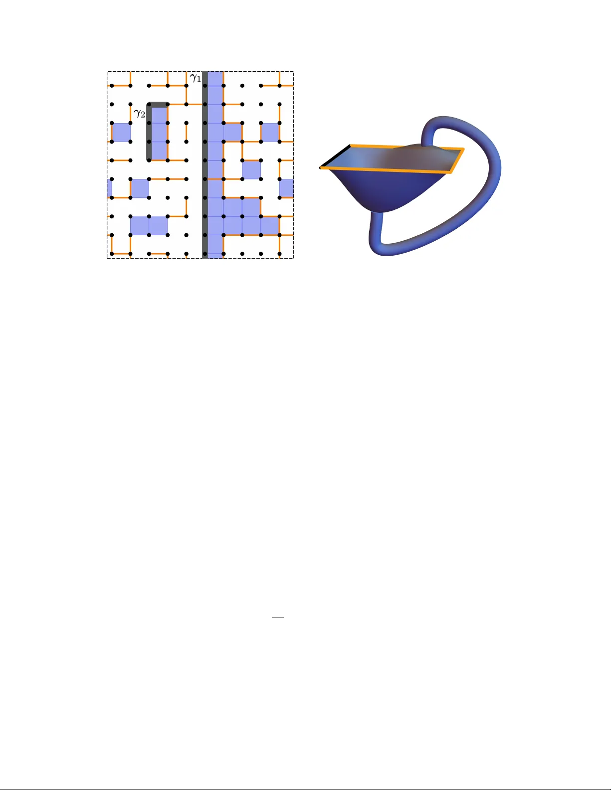
A CELLULAR REPRESENT A TION OF THE POTTS LA TTICE HIGGS MODEL SUMMER ELDRIDGE, MALIN P . F ORSSTR ¨ OM, AND BENJAMIN SCHWEINHAR T Abstract. The i -dimensional P otts lattice Higgs model is a random assignmen t of spins in Z q to the i -dimensional cells of a cell complex induced by a Hamiltonian with a Potts in teraction on the ( i + 1)-cells and an additional term pla ying the role of an external ﬁeld. W e dev elop a representation of this model as a pair of dependent plaquette p ercolations, and pro v e that Wilson line exp ectations can b e e xpressed in terms of the probability of a top ological even t. As an application, w e prov e the existence of a phase transition for the Marcu–F redenhagen ratio in the P otts lattice Higgs mo del on Z d when i = 1 . 1. Intr oduction Lattice Higgs mo dels, also called lattice gauge theories with matter, are a class of probabilit y distributions studied in ph ysics as discretized mo dels of gauge ﬁelds in the presence of particles [ FS79 ]. Mo dels with S U ( n )-v alued ﬁelds are of the greatest in terest, but simpler analogues are obtained b y taking spins in the integers mo dulo q ; the complexity is further reduced with a Potts interaction, as deﬁned in [ Bai88 ]. In the sp ecial case with Z 2 -v alued ﬁelds, these mo dels w ere already introduced in [ W eg71 ], as examples of spin mo dels with phase transitions and lo cal symmetries, and also app ear in quan tum information theory as natural noised version of Kitaevs toric co de, see, e.g., [ SSN21 ] W e will throughout refer to these mo dels as Potts lattice Higgs mo dels. In this pap er, w e dev elop an analogue of the F ortuin-Kasteleyn random cluster representation (see, e.g., [ FK72 ] for P otts lattice Higgs mo dels, b oth generalizing the random cluster represen tation of the P otts mo del with external ﬁeld [ Gri16 ] and building on recent work establishing a cellular represen tation of Potts lattice gauge theory [ DS25a , DS25b , Shk23 , HS16 ]. More sp eciﬁcally , we deﬁne a coupling b et w een the i -dimensional Potts lattice Higgs mo del — whic h assigns spins in Z q to the i -dimensional cells of a cell complex — and a new construction called c ouple d plaquette p er c olation (CPP), consisting of a dep enden t pair of plaquette p ercolations of dimensions ( i + 1) and i. W e pro ve that Wilson line exp ectations in the former can b e expressed in terms of the probability of a top ological even t in the latter. In addition, the CPP on Z d has a dualit y transformation deﬁned on the lev el of states; this giv es a concrete, geometric in terpretation of the dualit y of the partition functions of the P otts lattice Higgs mo del on Z 3 . As an application of the CPP , we pro ve the existence of a phase transition for the Marcu–F redenhagen ratio. T o simplify the argumen ts and k eep the required knowledge of algebraic top ology to a minim um, w e assume that q is prime and tak e free or p erio dic b oundary conditions; extensions to more general mo dels can b e obtained via mo diﬁcations similar to those in [ DS26 ]. Of particular interest is the case where i = 1 and X is a ﬁnite sub complex of the cubical complex Z d formed by tesselating Euclidean space with unit cub es. In this context, the P otts lattice Higgs mo del assigns spins to the edges with a Potts ﬁeld on the edges and a P otts in teraction on the signed sum of edges around 1 A CELLULAR REPRESENT A TION OF THE POTTS LA TTICE HIGGS MODEL 2 ev ery plaquette. The CPP is deﬁned on a pair of p ercolations: a 2-plaquette p ercolation P 2 and a b ond p ercolation P 1 , where the probabilit y is weigh ted by the size of the relative one-dimensional cohomology with co eﬃcien ts in Z q , denoted H 1 ( P 2 , P 1 ; Z q ). This coun ts the n umber of spin assignments to the edges of X that are compatible with the pair ( P 2 , P 1 ) in the sense that edges in P 1 are assigned spin 0 the oriented sum of spins around each plaquette of P 2 adds up to 0 mo dulo q . When d = 3 , the model is self-dual: there’s a bijective measure-preserving mapping b et ween the CPP and itself with diﬀeren t parameters. Sp ecial cases of the Ising lattice Higgs mo del include the Ising mo del with external ﬁeld ( i = 0 and q = 2) and the Ising lattice Higgs mo del ( i = 1 and q = 2) . The latter is an ob ject of previous study in b oth the ph ysics [ FS79 , HL91 , SSN21 , SPKL26 ] and in the mathematics [ F or24a , F or24b , F or25 ] literature. In particular, in [ F or24a ], it is sho wn that this mo del has a phase transition, which will b e extended to q  = 2 in this pap er. Alternate surface represen tations ha v e b een developed for these mo dels: a mem brane expansion obtained via a high temp erature expansion [ HL91 ] and a random current expansion [ FV25 , Aiz25 ]. In addition, w e note that the coupling b etw een the Ising lattice Higgs mo del and the CPP ma y b e of interest to ph ysicists studying the former mo del in computational exp erimen ts; it suggests a Swendsen–W ang-t yp e algorithm [ SW87 , ES88 , PDS25 ] whose dynamics may c hange along the phase boundaries and whic h ma y con v erge faster than other Mon te Carlo algorithms in practice. 1.1. Deﬁnitions and Notation. W e start by in tro ducing terminology and notation from algebraic top ology . The cell complex Z d is the tesselation of Euclidean space b y unit cub es with in tegter p oin ts as v ertices. Z d is comp osed of j -dimensional cells (called j -c el ls or j -plaquettes ) for 0 ≤ j ≤ d where the j -cells are the j -dimensional faces of cub es in the tesselation. That is, 0-cells are vertices, 1-cells are edges, 2-cells are unit squares, and so on. A j -dimensional subcomplex of Z d is a union of cells of Z d so that the dimension of eac h cell is at most j. Note that if σ is cell of a sub complex X and τ is a face of σ, then τ is also a cell of X . Another cell complex is the discrete torus T d N obtained from the sub complex [0 , N ] d of Z d b y identifying opp osite faces. F or a cell complex X denote b y X [ j ] the collection of all j -cells of X and the i -skeleton X ( j ) , the sub complex of X consisting of all cells of dimensions less than or equal to j. Giv en a cell complex X , w e notate b y C j ( X ; Z q ) the group of functions f from oriented j -cells in X to the additive group Z q of integers mo dulo q , with the prop ert y that if − x is x considered with the opp osite orien tation, f ( − x ) = − f ( x ). An elemen t of C j ( X ; Z q ) is called a “ j -c o chain ” or a “discrete j -form”. Dual to co c hains are chains whic h form the group C j ( X ; Z q ) of formal sums of oriented j -cells with co eﬃcien ts in Z q , with the relation that − x is obtained from x b y rev ersing the orientation. By extending linearly , we can ev aluate co c hains on chains. The c hain groups come with linear b oundary maps ∂ j : C j ( X ; Z q ) → C j − 1 ( X ; Z q ) deﬁned by ∂ j ( x ) = P y k , where y k are the set of orien ted ( j − 1)-cells incident to x . The linear c ob oundary maps δ j : C j ( X ; Z q ) → C j +1 ( X ; Z q ) are deﬁned b y δ j ( f )( x ) = f ( ∂ j +1 ( x )). Subscripts on the maps are generally omitted. The b oundary and cob oundary maps are used to deﬁned homology and cohomology , as describ ed at the b eginning of Section 2 b elo w. A CELLULAR REPRESENT A TION OF THE POTTS LA TTICE HIGGS MODEL 3 Deﬁnition 1 (Potts lattice Higgs Model) . Fix i ∈ Z ≥ 1 , q ∈ Z ≥ 2 , β 2 > 0 and β 1 > 0 , and let X b e a ﬁnite c el l c omplex. The Potts lattice Higgs model is the Gibbs me asur e µ = µ β 2 ,β 1 ,q ,i,X on C i ( X ; Z q ) induc e d by the Hamiltonian H ( f ) = − β 2 X σ ∈ X [ i +1] I 0 ( δ f ( σ )) − β 1 X ϵ ∈ X [ i ] I 0 ( f (  )) , wher e I x ( y ) is the indic ator that y = x. If i = 1 and q = 2 , 3 this mo del is equiv alent to the Z q lattice Higgs mo del with unitary gauge [FS79, F or24b] with Hamiltonian − β ′ 2 X σ ∈ X [2] Re e 2 πi q d f ( σ ) − β ′ 1 X ϵ ∈ X [1] Re e 2 πi q f ( ϵ ) . This follows from the fact that for q = 2 , 3, and x ∈ Z q , x 7→ Re e ( 2 πi q x ) is an aﬃne transformation of I 0 ( x ). W e note that there is an alternativ e deﬁnition of the Potts lattice Higgs Mo del [ Bai88 ] which assigns probabilities to a pair ( f , g ) with f ∈ C i ( X ; Z q ) and g ∈ C i − 1 ( X ; Z q ) . Sp eciﬁcally , one can consider the Gibbs measure ν induced by the Hamiltonian ˜ H ( f , g ) = − β ′ 2 X σ ∈ X [ i +1] I 0 ( δ f ( σ )) − β ′ 1 X ϵ ∈ X [ i ] I 0 ( f (  ) − δ g (  )) . (1) W e call ν the P otts lattice Higgs model with gener al gauge . F or an y h ∈ C i − 1 ( X ; Z q ), ν ( f , g ) is in v arian t under the gauge transformati on f → f + δ h, g → g + h . The map ( f , g ) → ( f − δ g , 0) co vers its image ev enly , so any function inv ariant under such a transformation (e.g. a Wilson line v ariable) will ha ve the same expectation in b oth mo dels. While Wilson line v ariables are not gauge in v ariant, the Wilson line expectation for µ equals the expectation of its analogue W ′ γ ( f , g ) : = exp  2 π i q ( f ( γ ) − g ( ∂ γ )  for ν (see, e.g., [F or24b]). Next, we deﬁne the CPP as a dep enden t pair of random p ercolation sub complexes. Deﬁnition 2 (P ercolation Sub complex) . A j -dimensional p ercolation sub complex of X is a sub c omplex P of X satisfying X ( j − 1) ⊆ P ⊆ X ( j ) . That is, P c ontains al l c el ls of dimension less than j and a subset of the the j -dimensional c el ls. When c onvenient, we tr e at a j -dimensional p er c olation sub c omplex P as a binary assignment to the j -c el ls, with P ( x ) = 1 iﬀ x ∈ P for x ∈ X [ j ] . We wil l write | P | for the numb er of j -c el ls of P . Deﬁnition 3. L et ( P 2 , P 1 ) b e a p air of p er c olation sub c omplexes, wher e the dimensions of P 2 and P 2 ar e ( i + 1) and i r esp e ctively. A n i -c o chain f ∈ C i ( X ; Z q ) is compatible with ( P 2 , P 1 ) if f (  ) = 0 for al l i -c el ls  of P 1 and δ f ( σ ) = 0 for al l ( i + 1) -c el ls σ of P 2 . A CELLULAR REPRESENT A TION OF THE POTTS LA TTICE HIGGS MODEL 4 The co c hains compatible with ( P 2 , P 1 ) form an additiv e group, the relative co cycle group, denoted Z i ( P 2 , P 1 ; Z q ) . As we will explain b elo w, this group coincides with the i -dimensional relativ e cohomology H i ( P 2 , P 1 ; Z q ) b ecause P 1 is a p ercolation sub complex. F or no w, w e only need that the symbol | H i ( P 2 , P 1 ; Z q ) | coun ts the n umber of compatible i -co c hains. Our cellular representation w eigh ts a pair of percolation sub complexes by this quantit y . Deﬁnition 4 (Coupled Plaquette P ercolation (CPP)) . F or a ﬁnite c el l c omplex X , a prime inte ger q , a non-ne gative inte ger i , and 0 ≤ p 2 , p 1 ≤ 1 deﬁne the Coupled Plaquette P ercolation me asur e ρ = ρ p 2 ,p 1 ,q ,i,X on p er c olation sub c omplexes P 2 and P 1 of dimensions ( i + 1) and i r esp e ctively, by ρ ( P 2 , P 1 ) ∝ p | P 2 | 2 (1 − p 2 ) | X [ i +1] |−| P 2 | p | P 1 | 1 (1 − p 1 ) | X [ i ] |−| P 1 |   H i ( P 2 , P 1 ; Z q )   . W e will often use the con venien t reparametrization k 2 = p 2 1 − p 2 and k 1 = p 1 1 − p 1 . In these co ordinates, the la w of the CPP ρ = ρ ( k 2 , k 1 , q, i, X ) is ρ ( P 2 , P 1 ) ∝ k | P 2 | 2 k | P 1 | 1   H i ( P 2 , P 1 ; Z q )   . The CPP has a n um b er of interesting sp ecial cases. When p 1 = 0, then P 2 is distributed as the ( i + 1)-dimensional plaquette random cluster mo del with co eﬃcients in Z q [ HS16 ]. Moreo ver, when X is simply connected and p 2 = 1, then P 1 is distributed as the i -dimensional PR CM with parameter p 1 . On the other hand, when either p 1 = 1 or p 2 = 0 the appropriate marginal distributions are indep enden t plaquette p ercolations (see Prop osition 20 b elo w). Fixing a states for either complex results in a random complex that can b e interpreted as a w eighted plaquette random cluster mo del. 1.2. Main Results. W e b egin by establishing the coupling b et ween the P otts lattice Higgs mo del and the CPP . Denote b y Ξ j = Ξ j ( X ) the collection of j -dimensional p ercolation sub complexes of X. Theorem 5. L et X b e a ﬁnite c el l c omplex, q b e a prime inte ger, and β 2 , β 1 ≥ 0 . If p 2 = 1 − e − β 2 , p 1 = 1 − e − β 1 , k 2 = p 2 1 − p 2 = e β 2 − 1 , and k 1 = p 1 1 − p 1 = e β 1 − 1 , then ther e is a c oupling κ = κ k 2 ,k 1 ,q ,i,X , κ : C i ( X ; Z q ) × Ξ i +1 × Ξ i → [0 , 1] , deﬁne d by κ ( f , P 2 , P 1 ) ∝ Y ϵ ∈ X [ i ] h I 0  P 1 (  )  + k 1 · P 1 (  ) · I 0  f (  )  i · Y σ ∈ X [ i +1] h I 0  P 2 ( σ )  + k 2 · P 2 ( σ ) · I 0  δ f ( σ )  i which satisﬁes the fol lowing. • The the mar ginal distribution on f is µ β 2 ,β 1 ,q ,i,X (the Potts lattic e Higgs mo del). • The mar ginal distribution on ( P 2 , P 1 ) is ρ p 2 ,p 1 ,q ,i,X (the CPP). • The c onditional distribution on ( P 2 , P 1 ) given f is indep endent p er c olation with pr ob a- bility p 2 on the set of ( i + 1) -c el ls so that δ f ( σ ) = 0 and pr ob ability p 1 on the set of i -c el ls such that f (  ) = 0 . • The c onditional distribution of f given ( P 2 , P 1 ) is the uniform me asur e on Z i ( P 2 , P 1 ; Z q ) . A CELLULAR REPRESENT A TION OF THE POTTS LA TTICE HIGGS MODEL 5 Figure 1. Two illustrations of the even t V γ . On the left, P 2 is depicted b y the collection of light blue squares and P 1 b y the orange b onds. The even ts V γ 1 and V γ 2 b oth o ccur, where γ 1 and γ 2 are the lo op and path sho wn in dark gra y . On the right, P 2 is shown by the blue surface and P 1 b y the orange line segmen t. γ is depicted in blac k. Here, V γ o ccurs when homology is taken with co eﬃcien ts in Z 2 but the plaquettes in the orange surface cannot b e compatibly orien ted to yield a n ull-homology when co eﬃcients are taken in a ﬁeld of o dd c haracteristic. The ﬁgure on the righ t w as adapted from Figure 1 of [ DS25a ] whic h w as in turn inspired b y Figure 1 of [A CC + 83]. The abov e coupling can b e mo diﬁed to provide a cellular represen tation of P otts lattice Higgs mo del in general gauge, as explained in Section 3.3 b elo w. In the sp ecial case i = 0 , the measure µ β 2 ,β 1 ,q ,i,X is the P otts mo del with external ﬁeld strength k 1 . T raditionally , the random cluster model is extended to a graphical represen tation of the Potts model with external ﬁeld via the in tro duction of a “ghost v ertex” [ Gri16 ]. W e describe wh y this is equiv alent to the i = 1 case of the CPP in Section 3.4. An imp ortable observ able in the P otts lattice Higgs mo del is the Wilson line observ able, whic h w e now deﬁne, together with a top ological ev en t whic h pro vides an analogue of the Wilson line observ able for the CPP . Deﬁnition 6 ( V γ and W γ ) . Fix an i -chain γ = P c j x j ∈ C i ( X ; Z q ) . F or f ∼ µ β 2 ,β 1 ,q ,i,X , we let W γ ( f ) b e the r andom variable exp  2 π i q f ( γ )  . If i = 1 , c j = 1 for al l j , and the e dges x j form a oriente d lo op, then W γ is r eferr e d to as a Wilson lo op v ariable . Similarly, if i = 1 , c j = 1 for al l j , and the e dges x j form an oriente d p ath, then W γ is r eferr e d to as a Wilson line v ariable . F or the me asur e ρ , V γ is the event that ther e exists an ( i + 1) -chain τ so that γ − ∂ τ is supp orte d on P 1 , or e quivalently that [ γ ] = 0 in H i ( P 2 , P 1 ; Z q ) (se e Figur e 1), wher e the r elative homolo gy H i ( P 2 , P 1 ; Z q ) is deﬁne d in Se ction 2 b elow. A CELLULAR REPRESENT A TION OF THE POTTS LA TTICE HIGGS MODEL 6 x n γ ′′ n y n γ ′ n n n/ 2 (a) The paths γ ′ n (solid) and γ ′′ n (dashed) app earing in the deﬁnition of the Marcu– F redenhagen ratio. n n/ 2 (b) The oriented surfaces q ′ n and q ′′ n that w ould b e natural to use in a deﬁnition of the MF ratio for i = 2 . Figure 2. In the ﬁgures abov e, w e dra w the paths and surfaces used in the deﬁnitions of the Marcu–F redenhagen ratio for i = 1 and i = 2 resp ectiv ely . Note that V γ is an increasing ev en t; adding more i -cells to P 1 increases the n um b er of i -c hains in C i ( P 1 ; Z q ), while adding more ( i + 1)-cells to P 2 increases the num b er of i -c hains that are b oundaries of ( i + 1)-c hains in C i +1 ( P 2 ; Z q ). Our next result expresses the exp ectation of a Wilson line observ able W γ in terms of the probabilit y of the ev ent V γ in the CPP . Observe that that taking the limit as β 1 → ∞ reco vers Theorem 5 of [DS25b]. Theorem 7. L et X b e a ﬁnite c el l c omplex, q b e a prime inte ger, β 2 , β 1 ≥ 0 , and γ ∈ C i ( X ; Z q ) . If µ = µ β 2 ,β 1 ,q ,i,X and ρ = ρ p 2 ,p 1 ,q ,i,X , wher e p 2 = 1 − e − β 2 and p 1 = 1 − e − β 1 , then E µ ( W γ ) = ρ ( V γ ) . Let µ β 2 ,β 1 ,q ,i, Z d b e the w eak limit of the measures µ β 2 ,β 1 ,q ,i, Λ N where Λ N = [ − N , N ] d (b y deﬁnition, these measures hav e free b oundary conditions). This inﬁnite volume limit exists b y standard argumen ts. Our arguments can easily b e extended to inﬁnite volume limits obtained from other b oundary conditions, but w e restrict atten tion to the free measure for simplicit y . W e sho w that for i = 1 the Potts lattice Higgs mo del exhibits a phase transition mark ed by a c hange in the b eha vior of a ratio b etw een Wilson line exp ectations. T o b e able to state this theorem, w e ﬁrst deﬁne an observ able in terms of the decomp osition of a lo op into tw o paths. Deﬁnition 8 (The Marcu–F redenhagen ratio for i = 1) . L et q b e a prime inte ger, i = 1 , and β 2 , β 1 ≥ 0 , and let µ = µ β 2 ,β 1 ,q ,i, Z d . F urther, let n ∈ 2 N and set γ n = ∂  [0 , n ] 2 × { 0 } d − 2 and let γ ′ n = γ ′ n ( R, T ) and γ ′′ n = γ ′′ n b e the p aths forme d by the upp er and lower halves of γ n (se e Figur e 2a). The Marcu–F redenhagen ratio is deﬁne d by A CELLULAR REPRESENT A TION OF THE POTTS LA TTICE HIGGS MODEL 7 β 2 β 1 Conﬁnemen t phase F ree phase Higgs phase R ( β 2 , β 1 , n ) ≳ 0 R ( β 2 , β 1 , n ) ≳ 0 R ( β 2 , β 1 , n ) ∼ 0 Figure 3. Conjectured limiting b eha vior of R ( β 2 , β 1 , n ) . W e will not address the diﬀerence b et ween the Conﬁnement phase and the Higgs phase here. W e prop ose to rigorously establish the diagram in the blue regions. R ( β 2 , β 1 , n ) = E µ ( W γ ′ n ) E µ ( W γ ′′ n ) E µ ( W γ n ) = E µ ( W γ ′ n ) 2 E µ ( W γ n ) . The quantit y R ( β 2 , β 1 , n ) is thought to b e relev ant to the physics of the Euclidean lattice Higgs mo del [ FM88 , BF85 ], and is predicted to exhibit a phase transition marked by whether or not its limit is zero (see Figure 3). The asymptotics of similar ratios where γ ′ n + γ ′′ n is tak en to b e a growing rectangular b oundary with a ﬁxed asp ect ratio are also of in terest, ev en in the case when γ ′ n and γ ′′ n do not ha ve equal length, and are conjectured to ha v e the same phase diagram [ Gli06 , FM88 , BF85 ]. Our argumen ts can be mo diﬁed to work in this con text. F or simplicit y , we assume that γ n is a square. W e note that by Theorem 7, w e can equiv alently deﬁne the Marcu–F redenhagen ratio using the equiv alen t top ological quan tity V γ . Deﬁnition 9 (The top ological Marcu–F redenhagen ratio) . L et q b e a prime inte ger, i = 1 , and p 2 , p 1 ∈ (0 , 1] , and let ρ = ρ p 2 ,p 1 ,q ,i, Z d . F urther, let ( γ ′ n , γ ′′ n ) b e as in Deﬁnition 8. The top ological Marcu–F redenhagen ratio is deﬁne d by ˆ R ( p 2 , p 1 , n ) = ρ ( V γ ′ n ) ρ ( V γ ′′ n ) ρ ( γ n ) = ρ ( V γ ′ n ) 2 ρ ( V γ n ) . One of the authors recen tly pro ved that the Marcu–F redenhagen ratio exhibits a non- trivial phase transition in the Z 2 lattice Higgs mo del [ F or24a ]; we will gain a more detailed understanding for the P otts lattice Higgs mo del as illustrated by the shaded regions in Figure 3. Theorem 10. L et q b e a prime inte ger, i = 1 , and β 2 , β 1 ≥ 0 , and let µ = µ β 2 ,β 1 ,q ,i, Z d . Consider the Mar cu–F r e denhagen r atio R as deﬁne d in Deﬁnition 8. Then the fol lowing holds. A CELLULAR REPRESENT A TION OF THE POTTS LA TTICE HIGGS MODEL 8 (1) If β 2 is suﬃciently lar ge, then ther e exists a β ′ 1 so that if β 1 < β ′ 1 , we have lim n →∞ R ( β 2 , β 1 , n ) = 0 . (2) If β 2 is suﬃciently smal l, then lim inf n →∞ R ( β 2 , β 1 , n ) > 0 . (3) If β 1 is suﬃciently lar ge, then lim inf n →∞ R ( β 2 , β 1 , n ) > 0 . In Prop osition 30, w e show that the natural analogue Marcu–F redenhagen ratio for i ≥ 2 (see Figure 2a) do es not exhibit a phase transition. The next few results elucidate the basic prop erties of the CPP . Theorem 11. ρ is p ositively asso ciate d. That is, if A and B ar e events that ar e incr e asing with r esp e ct to ( P 2 , P 1 ) then ρ ( A ∩ B ) ≥ ρ ( A ) ρ ( B ) . W e can compare the b eha vior of the CPP to a pair of indep endent plaquette p ercolations in the sense of sto chastic domination. Deﬁnition 12 (Sto chastic Domination) . F or a p air of binary assignments ω 1 , ω 2 , we say ω 1 ≤ ω 2 if for al l z , ω 1 ( z ) = 1 implies ω 2 ( z ) = 1 . If ther e exists a c oupling K ( ω 1 , ω 2 ) of two me asur es π 1 ( ω 1 ) , π 2 ( ω 2 ) so that K ( ω 1 ≤ ω 2 ) = 1 , we say π 2 sto chastic al ly dominates π 1 and write π 1 ≤ st π 2 . Theorem 13. L et X b e a ﬁnite c el l c omplex, q ≥ 1 , and p 2 , p 1 ∈ [0 , 1] . Then ρ p 2 ,p 1 is sto chastic al ly dominate d by indep endent Bernoul li p er c olation with pr ob abilities p 2 on ( i + 1) - c el ls and p 1 on i -c el ls, and sto chastic al ly dominates p er c olation with pr ob abilities p 2 q (1 − p 2 )+ p 2 and p 1 q (1 − p 1 )+ p 1 r esp e ctively. F urthermor e, when q is ﬁxe d, ρ is sto chastic al ly incr e asing in p 2 and in p 1 . In the text, we prov e a stronger version of Theorem 13, whic h concerns a mo diﬁed CPP where the cohomology co eﬃcients are no longer determined b y the parameter q . F or the next result, we sp ecialize the the d -dimensional torus; sp eciﬁcally , let T = T N d b e the discrete torus of length N obtained b y identifying opp osite faces of the cub e [0 , N ] d ⊂ Z d . Deﬁnition 14 (Bullet Dual) . If T is the d -dimensional unit cubic al lattic e on the torus, we let ( T ) • denote same lattic e, shifte d by 1 / 2 in every c o or dinate. F or every i -c el l x ∈ T , ther e is a unique ( d − i ) -c el l x ′ in ( T ) • . F or a set X , we deﬁne X • : = { x ′ ∈ ( T ) • | x / ∈ X } . Theorem 15. L et q b e a prime inte ger and let p 2 , p 1 ∈ [0 , 1] . Then ρ ( P 2 , P 1 ) = ρ • ( P • 1 , P • 2 ) , wher e p • 2 = q (1 − p 1 ) p 1 + q (1 − p 1 ) , p • 1 = q (1 − p 2 ) p 2 + q (1 − p 2 ) , ρ = ρ p 2 ,P 1 ,q ,i,d, T d N , and ρ • = ρ p • 2 ,p • 1 ,q ,d − i − 1 , ( T ) • . A CELLULAR REPRESENT A TION OF THE POTTS LA TTICE HIGGS MODEL 9 Analogues of Theorem 15 result can b e prov en with more general b oundary conditions. F or example, it is easy to mo dify the pro of to sho w that the dual of the mo del with free b oundary conditions has wired boundary conditions, when deﬁned appropriately (see, e.g., [ DS26 ]). When d − i − 1 = i , the P otts lattice Higgs mo del possesses a self-dual line in the 2-dimensional parameter space. While w e do not do so here, it would b e in teresting to consider how the coupling in Theorem 5 b eha ves under the duality transformation. This would yield a further generalization of the Lo op–Cluster coupling [ZMED20, HJK25]. W e outline the pap er. Section 2 reviews relev ant top ological background. Theorems 5 and 7 are pro ven in Section 3. This section also co v ers a coupling for the P otts lattice Higgs mo del in general gauge and the equiv alence of the CPP with the ghost v ertex construction. Sections 4.2, 4.3, and 4.4 include pro ofs of Theorems 11, 13, and 15, resp ectiv ely . In Section 5, we derive new and simple pro ofs of sev eral known prop erties of the P otts lattice Higgs Model: Griﬃth’s Second Inequality as well as a p erimeter law and monotonicity for Wilson line observ ables. Finally , Theorem 10 is prov en in Section 6. 2. Topological Terminology and Techniques Throughout the pap er, we rely hea vily on concepts from algebraic top ology . Standard references for these topics are [ Hat02 , Bre13 ], while [ KMM04 , Sa v16 ] provide in tro ductions sp eciﬁc to cubical complexes. 2.1. Absolute Homology and Cohomology. The b oundary and cob oundary maps deﬁned in Section 1.1 ha ve certain useful prop erties. Comp osing tw o b oundary maps, or tw o cob oundary maps, alwa ys gives the 0 map: ∂ j ◦ ∂ j +1 = 0 , δ j ◦ δ j − 1 = 0. Because im ∂ j +1 ⊂ k er ∂ j (also notated B j ( X ; Z q ) ⊂ Z j ( X ; Z q )) and im ∂ j +1 and k er ∂ j are b oth linear subspaces, w e can deﬁne the j -dimensional (absolute) homolo gy gr oup , H j ( X ; Z q ) = ker ∂ j / im ∂ j +1 . The cardinality of H j ( X ; Z q ) can very roughly b e interpreted as the the n umber of “linearly indep enden t holes” in the set: the kernel of the b oundary map are c hains with no b oundary , “ cycles ”, while the image are b oundaries , and the quotien t corresp onds to cycles that aren’t b oundaries. Quotien ting b y b oundaries not only remo ves cycles that are b oundaries, but also remo ves the distinction b et ween cycles whose only diﬀerence is a b oundary , lik e t wo nearby paths encircling the same lak e. Consider the cell complex X sho wn in Figure 4. It consists of six v ertices, seven oriented edges, and one face. W e may orient the face f 1 so that ∂ f 1 = e 1 + e 2 + e 3 + e 4 . The matrices of the b oundary maps ∂ 1 and ∂ 2 with resp ect to the ordered bases { v 1 , . . . , v 6 } of C 0 ( X ; Z q ) , { e 1 , . . . , e 7 } of C 1 ( X ; Z q ) , and { f 1 } for C 2 ( X ; Z q ) are ∂ 1 =        − 1 1 0 0 0 0 0 1 0 0 − 1 0 0 0 0 0 − 1 1 0 0 − 1 0 − 1 1 0 1 0 0 0 0 0 0 − 1 1 0 0 0 0 0 0 − 1 1        and ∂ 2 =          1 1 1 1 0 0 0          . A CELLULAR REPRESENT A TION OF THE POTTS LA TTICE HIGGS MODEL 10 f 1 e 4 e 7 e 6 e 5 e 2 e 1 e 3 v 2 v 3 v 6 v 1 v 4 v 5 Figure 4. A cell complex with six vertices, sev en edges, and one face. An elementary computation yields that Z 1 ( X ; Z q ) = ker ∂ 1 = Span ( e 1 + e 2 + e 3 + e 4 , e 3 − e 5 − e 6 − e 7 ) and B 1 ( X ; Z q ) = im ∂ 2 = Span ( e 1 + e 2 + e 3 + e 4 ) . Consequen tly , a basis for H 1 ( X ; Z q ) = Z 1 ( X ; Z q ) /B 1 ( X ; Z q ) is { e 3 − e 4 − e 6 − e 7 } , and thus H 1 ( X ; Z q ) ∼ = Z q . W e now deﬁne the c o cycles Z j ( X ; Z q ), the c ob oundaries B j ( X ; Z q ), and the c ohomolo gy H j ( X ; Z q ) , by Z j ( X ; Z q ) = ker δ j , B j ( X ; Z q ) = im δ j − 1 , and H j ( X ; Z q ) = ker δ j / im δ j − 1 . Then Z j ( X ; Z q ) consists of functions f ∈ C j ( X ; Z q ) suc h that f ( ∂ σ ) = 0 for all ( j + 1)-cells σ in X , B j ( X ; Z q ) consists of functions whic h can b e written as ∂ φ for some φ ∈ C j +1 ( X ; Z q ), and the cohomology H j ( X ; Z q ) consists of co cycles modulo cob oundaries. The cohomology is more diﬃcult to explain in tuitively , but can b e though t of as the “obstruction to discrete in tegrability” for the space X . Sp ecializing to the case where P 2 is an ( i + 1)-dimensional p ercolation sub complex, Z 1 ( P 2 ; Z q ) is the collection of spin assignments compatible with the pair ( ∅ , P 2 ) and B 1 ( P 2 ; Z q ) is the group of gauge symmetries. W e now return to the example in Figure 4. Cho osing bases { v ∗ 1 , . . . , v ∗ 6 } for C 0 ( X ) , { e ∗ 1 , . . . , e ∗ 7 } for C 1 ( X ; Z q ) , and { f ∗ 1 } for C 2 ( X ; Z q ), dual to the bases giv en ab o ve (where, for an i -cell σ the co c hain σ ∗ is deﬁned b y σ ∗ ( σ ′ ) = I σ = σ ′ ), we obtain matrices for the cob oundary maps δ 0 = ∂ T 1 and δ 1 = ∂ T 2 . In particular, it follo ws that Z 1 ( X ; Z q ) = Span ( e ∗ 1 − e ∗ 2 , e ∗ 1 − e ∗ 3 , e ∗ 1 − e ∗ 4 , e ∗ 5 , e ∗ 6 , e ∗ 7 ) and B 1 ( X ; Z q ) = Span ( − e ∗ 1 + e ∗ 2 , e ∗ 1 − e ∗ 4 , − e ∗ 3 + e ∗ 4 − e ∗ 7 , − e ∗ 2 + e ∗ 3 + e ∗ 5 , − e ∗ 5 + e ∗ 6 ) , and hence H 1 ( X ; Z q ) ∼ = Z q is a vector space of dimension one. There are man y c hoices of basis for this cohomology group, for example one could choose e ∗ 3 − e ∗ 4 − e ∗ 6 − e ∗ 7 . One could ask whether it is alw ays true that H 1 ( X ; Z q ) ∼ = H 1 ( X ; Z q ); this fails when q is non-prime and the simplest examples are embeddable in R 4 but not in R 3 . Here, we ﬁx q to b e prime so A CELLULAR REPRESENT A TION OF THE POTTS LA TTICE HIGGS MODEL 11 Z q is a ﬁeld, and the Univ ersal Co eﬃcien t Theorem for Cohomology (Theorem 3.2 in [ Hat02 ]) implies that in this case, H j ( X , A ; Z q ) ∼ = H j ( X , A ; Z q ) for all j . One migh t be tempted to b eliev e that the dimensions of the vector spaces H j ( X ; Z q ) and H j ( X ; Z q ) do not dep end on q . Ho wev er, while this is true for j = 0 , it is false for j > 0 . The simplest examples for whic h this fails are non-orientable surfaces suc h as the real pro jective plane and Klein b ottle. When we are not relying on particular prop erties of the co eﬃcien t ﬁeld, we usually suppress it for brevit y and write, e.g., C j ( X ) instead of C j ( X ; Z q ) , but w e will note whenever it is relev ant. 2.2. Relativ e Homology and Cohomology. Homology and cohomology apply to a single complex X . Ho wev er, we can p erform a similar process for a pair of complexes ( X , A ), where A is a sub complex of X . F or so-called “go o d pairs” ( X , A ) , the r elative homolo gy H j ( X , A ) and r elative c ohomolo gy H j ( X , A ) are respectively isomorphic to the absolute homology H j ( X/ A ) and absolute cohomology H j ( X/ A ) of the quotien t space X/ A formed b y collapsing A to a single p oin t (where w e are suppressing the dep endence on the c hoice of co eﬃcien ts). See Theorem 2.13 in [ Hat02 ] for the statemen t of this result for homology and the discussion b elo w for the deﬁnition of a go o d pair. The pro of for cohomology pro ceeds iden tically . While all pairs considered in this paper are deterministically go o d, it will b e useful to pro vide an equiv alent deﬁnition via relativ e c hain and co c hain groups. The relativ e chain group is the quotien t v ector space C j ( X , A ) = C j ( X ) /C j ( A ). As the b oundary of a c hain supp orted on A is also supp orted on A, the usual b oundary map induces a relative b oundary map ∂ j : C j ( X , A ) → C j − 1 ( X , A ), and w e can deﬁne relative homology H j ( X , A ) = k er ( ∂ j ) / im ( ∂ j +1 ) . On the other hand, the relativ e co chain group C j ( X , A ) is the subspace of C j ( X ) consisting of cochains that v anish on all j -cells of A and the relativ e cob oundary map δ j is the restriction of the absolute cob oundary map to C j ( X , A ) . Again, H j ( X , A ) = k er δ j / im δ j − 1 . In our setting, the relative cohomology is muc h simpler. If P 2 and P 1 are a pair of p ercolation sub complexes of dimensions ( i + 1) and i, then they share the same ( i − 1)-cells so C i − 1 ( P 2 , P 1 ) = 0 . Th us H i ( P 2 , P 1 ) = k er ( δ i ( C i ( P 2 , P 1 ))) : = Z i ( P 2 , P 1 ) , whic h is simply the set of relativ e co-cycles: co c hains compatible with ( P 2 , P 1 ) in the sense of Deﬁnition 3. Returning to the example X in Figure 4, if w e set A to contain all cells of X except e 5 , e 6 , and e 7 then C 0 ( X , A ) = { 0 } , C 1 ( X , A ) = Span ( e ∗ 5 , e ∗ 6 , e ∗ 7 ) , and C 2 ( X , A ) = { 0 } . It follows that H 1 ( X , A ) = C 1 ( X , A ) ∼ = Z 3 q . Alternativ ely , the quotient space X/ A consists of three circles meeting at a p oin t, and it is easily seen that H 1 ( X/ A ) ∼ = H 1 ( X/ A ) ∼ = Z 3 q . Since q is a prime num b er, H j ( X , A ; Z q ) and H j ( X , A ; Z q ) are vector spaces (as quotien ts of vector spaces) and are determined by their dimensions. Deﬁnition 16 (Betti n umbers) . The j -dimensional relativ e Betti n umber is b j ( X , A ; Z q ) : = rank  H j ( X , A ; Z q )  = rank  H j ( X , A ; Z q )  . By applying the rank-n ullit y theorem to the b oundary maps, w e obtain the famous Euler– Poinc ar´ e formula . A CELLULAR REPRESENT A TION OF THE POTTS LA TTICE HIGGS MODEL 12 Prop osition 17. If X is a ﬁnite, d -dimensional c el l c omplex and q is a prime numb er then χ ( X ) : = d X j =0 ( − 1)) j | X [ j ] | = ( − 1) j b j ( X , A ; Z q ) . 2.3. May er–Vietoris Sequences. In this section, w e describ e the May er–Vietoris sequence for cohomology , a key tec hnical to ol that relates the relativ e cohomology of a pair of spaces with that of their union and their intersection [ Hat02 , pp 149–153 and 203–204]. W e will apply the May er–Vietoris sequence to pro v e that the CPP is p ositively associated in Section 4.2 and to demonstrate a tec hnical lemma in Section 6. A reader may wish to skip this section for now. While we apply the Ma yer–Vietoris sequence for relative cohomology b elo w, we b egin by describing the sequence for absolute cohomology for the purp ose of simplicit y . T o this end, note ﬁrst that if P and Q are tw o cell complexes with P ⊂ Q , then the inclusion map P  → Q induces a restriction map H j ( Q ) → H j ( P ) that sends the homology class [ f ] of a co cycle f supp orted on Q to the cohomology class [ f | P ] of its restriction to P . No w, supp ose that P and Q are sub complexes of the same cell complex. W e obtain four diﬀeren t restriction maps on cohomology φ P : H j ( P ) → H j ( P ∩ Q ) , φ Q : H j ( Q ) → H j ( P ∩ Q ) , ψ P : H j ( P ∪ Q ) → H j ( P ) , and ψ Q : H j ( P ∪ Q ) → H j ( Q ) . These maps ﬁt together in a sequence H j ( P ∩ Q ) ϕ P − ϕ Q ← − − − H j ( P ) ⊕ H j ( Q ) ψ P ⊕ ψ Q ← − − − H j ( P ∪ Q ) . (2) with the follo wing prop erties. (1) If [ f ] ⊕ [ g ] ∈ im( ψ P ⊕ ψ Q ), then φ P ([ f ]) − φ Q ([ g ]) = 0 . (2) In fact, the conv erse implication also holds: if φ P ([ f ]) − φ Q ([ g ]) = [0] , then there is an h ∈ C j − 1 ( P ∩ Q ) so that δ h + f | P ∩ Q = g | P ∩ Q . The map h can b e extended b y zero to deﬁne a co c hain on all of P so we ma y replace f with f + δ h if necessary to ﬁnd a representativ e of the same cohomology class of P so that f | P ∩ Q = g | P ∩ Q . Then w e can deﬁne F ∈ C i ( P ∪ Q ) b y F ( σ ) = f ( σ ) if σ ∈ P and F ( σ ) = g ( σ ) otherwise. Since f and g are co cycles on P and Q, it follows that F is a co cycle supp orted on P ∪ Q, and hence [ f ] ⊕ [ g ] ∈ im( ψ x ⊕ ψ Q ) . Com bining the ab ov e observ ations, it follows that the sequence in 2 is exact , i.e., that ψ P ⊕ ψ Q ( F ) = f ⊕ g and im ψ P ⊕ ψ Q = k er ( φ P − φ Q ) . This is not quite enough to compute the cohomology groups of P ∪ Q in terms of those of P , Q , and P ∩ Q ; we also require kno wledge of the image of φ P − φ Q and the k ernel of ψ P ⊕ ψ Q . It turns out that the cob oundary map pro vides the required information. Sp eciﬁcally , it induces a map δ ∗ : H j ( P ∩ Q ) → H j +1 ( P ∩ Q ) so that the following sequence is exact in the sense that the image of eac h map is the kernel of the next: · · · H j ( P ∩ Q ) H j ( P ) ⊕ H j ( Q ) H j ( P ∪ Q ) H j − 1 ( P ∩ Q ) · · · · · · H 0 ( P ∪ Q ) 0 . δ ∗ ϕ P − ϕ Q ψ P ⊕ ψ Q δ ∗ δ ∗ ϕ P − ϕ Q ψ P ⊕ ψ Q A CELLULAR REPRESENT A TION OF THE POTTS LA TTICE HIGGS MODEL 13 W e will not use the precise construction of δ ∗ here, only that the sequence is exact. This construction extends to relativ e cohomology . Assume that A and B are sub complexes of P and Q, resp ectiv ely . Then, the May er–Vietoris sequence for relative cohomology is as follo ws. · · · H j ( P ∩ Y , A ∩ B ) H j ( P , A ) ⊕ H j ( Y , B ) H j ( P ∪ Y , A ∪ B ) H j − 1 ( P ∩ Y , A ∩ B ) · · · · · · H 0 ( P ∪ Y , A ∪ B ) 0 . 2.4. Alexander Duality. Alexander dualit y relates the homology of a subset of Euclidean space with the cohomology of its complemen t. It generalizes the top ological fact that the n umber of linearly indep enden t lo ops of a b ounded subset X of R 2 equals the n umber of b ounded comp onen ts of the complemen t R 2 ∖ X . If A ⊂ X is contained in an orientable compact d -dimensional manifold S , where A is closed and X is compact, this can b e further generalized to relate the relativ e homology of the pair ( X , A ) with the relative cohomology of ( S ∖ A, S ∖ X ) [Spa66, Theorem 6.2.17]: H j ( S ∖ A, S ∖ X ; Z q ) ∼ = H d − j ( X , A ; Z q ) . F or example, if X is a compact subset of R 2 , and A ⊂ X con tains a single non-con tractible lo op then the rank of H 1 ( X , A ) will b e one less than the rank of H 1 ( X ) , and H 1 ( R 2 ∖ A, R 2 ∖ X ) will also ha ve rank one less than H 1 ( R 2 ∖ A, R 2 ∖ X ) . 3. The coupling between the CPP and the Potts la ttice Higgs model In this section, we prov e Theorem 5 and discuss some of its consequences. 3.1. Deriv ation of the Coupling. F or clarit y of notation: σ alw ays refers to an ( i + 1)- cell,  alw ays refers to an i -cell, j -cells contained within a giv en j -dimensional p ercolation sub complex are called “op en”, and are otherwise called “closed.” Pr o of of The or em 5 . W e ﬁrst compute the marginals of κ ( f , P 2 , P 1 ) . T o this end, note ﬁrst that κ 1 ( f ) : = X P 1 X P 2 κ ( f , P 2 , P 1 ) ∝ X P 1 X P 2 h Y ϵ ∈ X [ i ] h I 0  P 1 (  )  + k 1 P 1 (  ) I 0  f (  )  i Y σ ∈ X [ i +1] h I 0  P 2 ( σ )  + k 2 P 2 ( σ ) I 0  δ f ( σ )  i i . Changing the order of the sums and pro ducts, it follows that the previous expression is equal to Y ϵ ∈ X [ i ] h 1 + k 1 I 0  f (  )  i Y σ ∈ X [ i +1] h 1 + k 2 I 0  δ f ( σ )  i = Y ϵ ∈ X [ i ] h 1 + ( e β 1 − 1) I 0  f (  )  i Y σ ∈ X [ i +1] h 1 + ( e β 2 − 1) I 0  δ f ( σ )  i = Y ϵ ∈ X [ i ] e β 1 I 0 ( f ( σ )) Y σ ∈ X [ i +1] e β 2 I 0 ( δ f ( σ )) . A CELLULAR REPRESENT A TION OF THE POTTS LA TTICE HIGGS MODEL 14 Next, for the second marginal, we hav e κ 2 ( P 2 , P 1 ) : = X f κ ( f , P 2 , P 1 ) ∝ X f h Y ϵ ∈ X [ i ] h I 0  P 1 (  )  + k 1 P 1 (  ) I 0  f (  )  i Y σ ∈ X [ i +1] h I 0  P 2 ( σ )  + k 2 P 2 ( σ ) I 0  δ f ( σ )  i i = k 1 | P 1 | k 2 | P 2 | X f Y ϵ : P 1 ( ϵ )=1 I 0  f ( σ )  Y σ : P 2 ( σ )=1 I 0  δ f ( σ )  = k 1 | P 1 | k 2 | P 2 |    f : ∀  ∈ P 1 , f (  ) = 0 , ∀ σ ∈ P 2 , δ f ( σ ) = 0    ∝ (1 − p 1 ) | X [ i ] |−| P 1 | p | P 1 | 1 (1 − p 2 ) | X [ i +1] |−| P 2 | p | P 2 | 2 ·    f : ∀  ∈ P 1 , f (  ) = 0 , ∀ σ ∈ P 2 , δ f ( σ ) = 0    . (3) Since Z i ( P 2 , P 1 ) = { f : ∀ , f (  ) = 0 , ∀ σ, δ f ( σ ) = 0 } , and, as w e mentioned in Section 2, we ha ve H i ( P 2 , P 2 ) = Z i ( P 2 , P 1 ), it follo ws that κ 2 ( P 2 , P 1 ) ∝ (1 − p 1 ) | X [ i ] |−| P 1 | p | P 1 | 1 (1 − p 2 ) | X [ i +1] |−| P 2 | p | P 2 | 2 | H i ( P 2 , P 1 ; Z q ) | . No w w e derive the conditional distributions of κ ( f , P 2 , P 1 ). T o this end, note ﬁrst that κ ( f | P 2 , P 1 ) ∝ Y ϵ ∈ X [ i ] h I 0  P 1 (  )  + k 1 P 1 (  ) I 0  f (  )  i Y σ ∈ X [ i +1] h I 0  P 2 ( σ )  + k 2 P 2 ( σ ) I 0  δ f ( σ )  i = Y ϵ : P 1 ( ϵ )=1 hI 0 ( f (  )) Y σ P 2 ( σ )=1 K I 0 ( δ f ( σ )) . In other words, given P 1 and P 2 , if either δ f ( σ )  = 0 for some σ ∈ P 2 or f (  )  = 0 for some  ∈ P 1 , then κ ( f | P 2 , P 1 ) = 0 , and otherwise, the distribution of κ ( · | P 2 , P 1 ) is uniform. F or the other conditional marginal distribution, we hav e κ ( P 2 , P 1 | f ) ∝ Y ϵ ∈ X [ i ] h I 0  P 1 (  )  + k 1 P 1 (  ) I 0  f (  )  i · Y σ ∈ X [ i +1] h I 0  P 2 ( σ )  + k 2 P 2 ( σ ) I 0  δ f ( σ )  i = Y ϵ : f ( ϵ )=0 h I 0  P 1 (  )  + k 1 P 1 (  ) i Y ϵ : f ( ϵ )  =0 I 0  P 1 (  )  · Y σ : δ f ( σ )=0 h I 0  P 2 ( σ )  + k 2 P 2 ( σ ) i Y σ : δ f ( σ )  =0 I 0  P 2 ( σ )  ∝ Y ϵ : f ( ϵ )=0 h (1 − p 1 ) I 0  P 1 (  )  + p 1 P 1 (  ) i Y ϵ : f ( ϵ )  =0 I 0  P 1 (  )  · Y σ : δ f ( σ )=0 h (1 − p 2 ) I 0  P 2 ( σ )  + p 2 P 2 ( σ ) i Y σ : δ f ( σ )  =0 I 0  P 2 ( σ )  . A CELLULAR REPRESENT A TION OF THE POTTS LA TTICE HIGGS MODEL 15 In w ords, the i -cells on whic h f v anishes and the ( i + 1) cells on whic h δ f is zero are included indep enden tly . This concludes the pro of. □ 3.2. T op ological In terpretation of Wilson Line Observ ables. In this section, we apply the coupling from Theorem 5 to express Wilson line exp ectations to b e expressed in terms of the probability of a top ological even t in the CPP . Pr o of of The or em 7 . It suﬃces to sho w that E κ ( W γ | V γ ) = 1 and E κ ( W γ | V c γ ) = 0 . T o this end, ﬁx γ , P 2 , and P 1 , and let f ∼ κ ( · | P 2 , P 1 ) . If [ γ ] = 0, then γ = σ + ∂ τ for some σ ∈ C i ( P 1 ) and τ ∈ C i +1 ( P 2 ). Since f is sampled uniformly from Z i ( P 2 , P 1 ; Z q ), we ha v e f ( γ ) = f ( σ ) + f ( ∂ τ ) = f ( σ ) + δ f ( τ ) = 0 + 0 = 0 , where we used that f v anishes on P 1 and δ f v anishes on P 2 . Thus W γ = exp  2 π i q f ( γ )  = 1 . The conditional distribution of f giv en ( P 2 , P 1 ) can be sampled by ﬁxing a basis { f 1 , . . . , f k } of the vector space H i ( P 2 , P 1 ; Z q ) , letting a 1 , . . . , a k b e distributed indep enden tly and uniformly on Z q , and setting f = a 1 f 1 + . . . a k f k . No w assume [ γ ]  = 0. By the Univ ersal Co eﬃcien t Theorem there exists a dual [ γ ] ∗ ∈ H i ( P 2 , P 1 ; Z q ) so that [ γ ] ∗ ([ γ ]) = 1 . In particular, f j ([ γ ])  = 0 for at least one index j . By m ultiplying eac h basis elemen t by a non-zero element of Z q w e ma y assume, without loss of generalit y , that f j ( γ ) = 1 for 1 ≤ j ≤ m and f j ( γ ) = 0 otherwise. Then f ( γ ) = a 1 + . . . + a m is a sum of i.i.d. uniform elements of Z q , and is itself uniformly distributed on Z q . This implies in particular that E κ ( W γ | V c γ ) = 0 , whic h is the desired conclusion. □ 3.3. Potts Lattice Higgs in General Gauge. The pro of of Theorem 5 can b e mo diﬁed in a straigh tforw ard fashion to pro duce a coupling b et ween the CPP and the Potts lattice Higgs mo del in general gauge. Recall that ν = ν β 2 ,β 1 ,q ,i is the measure induced b y the Hamiltonain in (1). Corollary 18. Under the assumptions of The or em 5, ther e is a c oupling ˆ κ = ˆ κ k 2 ,k 1 ,i,q , with ˆ κ : ( C i ( X ; Z q ) × C i − 1 ( X ; Z q )) × (Ξ i +1 × Ξ i ) → [0 , 1] , deﬁne d by ˆ κ (( f , g ) , ( P 2 , P 1 )) ∝ Y ϵ ∈ X [ i ] h I 0  P 1 (  )  + k 1 · P 1 (  ) · I δ g ( ϵ )  f (  )  i · Y σ ∈ X [ i +1] h I 0  P 2 ( σ )  + k 2 · P 2 ( σ ) · I 0  δ f ( σ )  i which satisﬁes the fol lowing. A CELLULAR REPRESENT A TION OF THE POTTS LA TTICE HIGGS MODEL 16 • The mar ginal distribution on ( f , g ) is ν β 2 ,β 1 ,q ,i,X (the Potts lattic e Higgs mo del in gener al gauge). • The mar ginal distribution on ( P 2 , P 1 ) is ρ p 2 ,p 1 ,q ,i,X (the CPP). • The c onditional distribution on ( P 2 , P 1 ) given ( f , g ) is, r esp e ctively, indep endent p er c olation with pr ob ability p 2 on the set of ( i + 1) -c el ls so that δ f ( σ ) = 0 and pr ob ability p 1 on the set of i -c el ls so that f (  ) = δ g (  ) . • The c onditional distribution of f given ( P 2 , P 1 ) and g is the uniform distribution on the set δ g + Z i ( P 2 , P 1 ; Z q ) and the c onditional distribution of g given ( P 2 , P 1 ) is uniform on C i − 1 ( X ; Z q )) . Note that while δ g is necessarily an element of Z i ( P 2 ; Z q ) , it ma y not b e a member of of Z i ( P 2 , P 1 ; Z q ) . Pr o of. The pro of structure is very similar to that of Theorem 5. W e note only the c hanges. T o compute the marginal on ( f , g ) it suﬃces to simply replace I 0 ( f (  )) with I δ g ( ϵ ) ( f (  )) in the computation of the marginal of κ on f . F or the marginal ˆ κ 2 ( P 2 , P 1 ) : = X f ,g κ  ( f , g ) , ( P 2 , P 1 )  on ( P 2 , P 1 ), the pro of pro ceeds identically as in (3) except that the factor  f | ∀ , f (  ) = 0 , ∀ σ, δ f ( σ ) = 0  =   Z i ( P 2 , P 1 ; Z q )   in the ﬁnal line is replaced with X g ∈ C i − 1 ( X )   { f | ∀ , f (  ) = δ g (  ) , ∀ σ, δ f ( σ ) = 0 }   , whic h in turn equals | C i − 1 ( X ) | × | Z i ( P 2 , P 1 ; Z q ) | since the summand do es not depend on g . Th us ˆ κ 2 ( P 2 , P 1 ) = | C i − 1 ( X ) | κ 2 ( P 2 , P 1 ) ∝ κ 2 ( P 2 , P 1 ) ∝ ρ ( P 2 , P 1 ) . F or the conditional distribution of ( f , g ) given ( P 2 , P 1 ), we again plug in I δ g ( ϵ ) ( f (  )), to get that the probabilit y is 0 if for any σ ∈ P 2 , δ f ( σ )  = 0 or an y  ∈ P 1 , f (  )  = δ g (  ), and otherwise uniform. Because the num b er of such f is not dep enden t on g , we can select g ﬁrst b y indep enden t choices from Z q on each ( i − 1)-cell, uniformly choose a co cycle h , and then deﬁne f as h + δ g . F or the conditional of ( P 2 , P 1 ) giv en ( f , g ), we con tinue to substitute I δ g ( ϵ ) ( f (  )), which results in probabilit y 0 if P 1 (  ) = 1 for an y  so that f (  )  = δ g (  ) or P 2 ( σ ) = 1 for an y σ so that d f ( σ ) = 0, and is, as ab o v e, otherwise indep endent p ercolation. □ 3.4. Equiv alence with the Ghost V ertex Construction. In this section, we explain why the i = 0 case of the CPP is equiv alent to the graphical representation of the Potts model with external ﬁeld obtained b y introducing a “ghost v ertex” to the random cluster mo del. T o this end, let G b e a graph and denote by G ′ the graph obtained b y adding one additional “ghost” vertex g to the v ertex set of G and an edge e v = ( v , g ) for each v ertex v of G. Also, A CELLULAR REPRESENT A TION OF THE POTTS LA TTICE HIGGS MODEL 17 for f ∈ C 0 ( G ; Z q ) , let f ′ ∈ C 0 ( G ′ ; Z q ) b e the “extension by 0” of f ; that is f ′ ( v ) = f ( v ) for any v ertex v of G and f ′ ( g ) = 0. Moreov er, for an edge e , let p ( e ) = ( p 2 : = k 2 1+ k 2 if e ∈ E ( G ) , and p 1 : = k 1 1+ k 1 if e / ∈ E ( G ) . Deﬁne a coupling κ ′ = κ ′ k 2 ,k 1 ,q ,G , κ ′ : C 0 ( G ; Z q ) × Ξ 1 ( G ′ ) → [0 , 1] b y κ ′ ( f , P ) ∝ Y e =( g ,v ) h (1 − p 1 ) I 0 ( P ( e )) + p 1 P ( e ) I 0  δ f ′ ( e )  i · Y e ∈ E ( G ) h (1 − p 2 ) I 0  P ( e )  + p 2 P ( e ) I 0  δ f ′ ( e )  i . That is, κ ′ is obtained from the usual coupling b et ween the random cluster mo del on G ′ (with t w o diﬀeren t t yp es of edges) and the P otts mo del on G ′ conditioned on f ′ ( g )) = 0. Prop osition 19. Assume the hyp otheses of The or em 5 with X = G. L et P 1 ∈ Ξ 0 ( G ) and P 2 ∈ Ξ 1 ( G ) and let P ∈ Ξ 1 ( G ′ ) b e obtaine d fr om P 2 by adding al l e dges of the form ( v , g ) wher e v ∈ P 1 . Then κ ( f , P 2 , P 1 ) = κ ′ ( f ′ , P ) wher e κ ′ = κ ′ ( k 2 , k 1 , q , G ) . In p articular, µ ( f ) = µ ′ ( f ′ ) wher e µ ′ is the usual Potts me asur e on G ′ c onditione d on f ( g ) = 0 , and ρ ( P 2 , P 1 ) = ρ ′ ( P ′ ) , wher e ρ ′ is the r andom cluster me asur e with pr ob ability p 2 assigne d to e dges in G and p 1 assigne d to e dges in G ′ \ G. Pr o of. First, note that f is in bijectiv e corresp ondence with f ′ , and ( P 2 , P 1 ) is in bijective corresp ondence with P ′ . Th us, the statement is immediate if the asso ciated w eigh ts are prop ortional. W e ha ve that κ ( f , P 2 , P 1 ) ∝ Y v ∈ X [0] h I 0  P 1 ( v )  + k 1 · P 1 ( v ) · I 0  f (  )  i · Y e ∈ X [1] h I 0 ( P 2 ( e )) + k 2 · P 2 ( e ) · I 0 ( δ f ( e )) i . If e = ( g , v ), then P 1 ( v ) = P ′ ( e ), and I 0 ( f ( e )) = I 0 ( δ f ′ ( e )). Similarly , if e ∈ E ( G ), P ′ ( e ) = P 2 ( e ) and δ f ′ ( e ) = δ f ( e ). Dividing eac h term by (1 − p 1 ) | X [0] | (1 − p 2 ) | X [1] | yields κ ′ ( f ′ , P ′ ) ∝ Y e =( g ,v ) h I 0  P ′ ( e )  + p 1 1 − p 1 P ′ ( e ) I 0  δ f ′ ( e )  i · Y e ∈ E ( G ) h I 0  P ′ ( e )  + p 2 1 − p 2 P ′ ( e ) I 0  δ f ′ ( e )  i . Since k 2 = p 2 1 − p 2 and k 1 = p 1 1 − p 1 , this concludes the pro of. □ 4. Pr oper ties of the CPP W e establish a n umber of basic prop erties of Coupled Plaquette Percolation. A CELLULAR REPRESENT A TION OF THE POTTS LA TTICE HIGGS MODEL 18 4.1. Sp ecial Cases of the CPP. Let X b e a ﬁnite cell complex. The i -dimensional plaquette random cluster mo del [ HS16 , DS25a , Shk23 ] with parameters p ∈ [0 , 1] and q ∈ N ≥ 2 is the random i -dimensional p ercolation sub complex of X whose probability is w eighted b y the absolute ( i − 1)-homology with co eﬃcien ts in Z q . Sp eciﬁcally , deﬁne ˆ ρ = ˆ ρ p,q ,i,X b y ˆ ρ ( P ) ∝ p | P | (1 − p ) | X [ i ] |−| P |   H i − 1 ( P ; Z q )   . The deﬁnition of ˆ ρ is extended to q = 1 by setting ˆ ρ p, 1 ,i,X ∝ p | P | (1 − p ) | X [ i ] |−| P | . That is, the q = 1 case of the plaquette random cluster mo del is Bernoulli plaquette p ercolation. This naturally o ccurs as the q → 1 limit of a related mo del where the choice of cohomology co eﬃcien ts is in some sense decoupled from the choice of q in exactly the same fashion as the auxiliary mo del deﬁned in Section 4.3 b elo w. Let π 2 p 2 ,p 1 ,q ,i,X and π 1 p 2 ,p 1 ,q ,i,X b e the marginal distributions of P 2 and P 1 when ( P 2 , P 1 ) ∼ ρ p 2 ,p 1 ,q ,i,X . By deﬁnition, π 2 p 2 , 0 ,q ,i,X has the distribution of the plaquette random cluster mo del, and π 2 p 2 , 0 , 1 ,i,X d = ˆ ρ p,i +1 ,X . Our next result, Prop osition 20, collects t w o other sp ecial cases. Prop osition 20. If X is a ﬁnite c el l c omplex then π 2 p 2 , 0 ,q ,i,X d = ˆ ρ p 2 ,q ,i +1 ,X , π 2 p 2 , 1 ,q ,i,X d = ˆ ρ p 2 , 1 ,i +1 ,X , and π 1 0 ,p 1 ,q ,i,X d = ˆ ρ p ∗ ( p,q ) , 1 ,i,X , wher e p ∗ ( p, q ) = p q − pq + p . In addition, if X satisﬁes H i − 1 ( X ; Z q ) = H i ( X ; Z q ) = 0 then π 1 1 ,p 1 ,q ,i,X d = ˆ ρ p 1 ,q ,i,X . Pr o of. Since the presence or absence of j -cells in X for j > i + 1 do es not inﬂuence the distribution of ρ , we may assume that X = X ( i +1) . The ﬁrst claim follows from the observ ation that H i ( P 2 , X ( i − 1) ) = Z i ( P 2 ) so   H i ( P 2 , X ( i − 1) )   =   Z i ( P 2 )   =   H i ( P 2 )     B i ( P 2 )   ∝   H i ( P 2 )   since B i ( P 2 ) = B i ( X ) do es not dep end on P 2 . T o obtain the second claim, note that the only co chain compatible with  P 2 , X ( i )  is identically zero so H i ( P 2 , X ( i ) ) = 0 . F or the third claim, note that when P 2 con tains no ( i + 1)-cells, the only constrain t on compatible i -co chains is that they v anish on the i -cells of P 1 . Thus   H i ( X ( i ) , P 1 )   =   C i ( X , P 1 )   = q | X [ i ] |−| P 1 | , and hence ρ 0 ,p 1 ,q ,i,X ( X ( i ) , P 1 ) ∝  p 1 1 − p 1  | P 1 | q | X ( i ) |−| P 1 | ∝  p ∗ ( p, q ) 1 − p ∗ ( p, q )  | P 1 | = ρ p ∗ ( p,q ) , 0 , 1 ,i − 1 ,X . A CELLULAR REPRESENT A TION OF THE POTTS LA TTICE HIGGS MODEL 19 T o pro ve the fourth claim, w e will demonstrate that H i − 1 ( P 1 ) ∼ = H i ( X , P 1 ) . Readers familiar with algebraic top ology will recognize that the follo wing argumen t is an application of the long exact sequence of a pair. Let f ∈ Z i − 1 ( P 1 ) and consider the cob oundary δ f . δ f v anishes on eac h i -cell of P 1 b y deﬁnition and δ ( δ f ) = 0 so δ f ∈ Z i ( X , P 1 ) = H i ( X , P 1 ) . Since δ ◦ δ = 0 , δ sends each elemen t of the homology class of f to the same homology class in H i ( X , P 1 ) . That is, the cob oundary map induces a w ell-deﬁned map δ ∗ : H i − 1 ( P 1 ) → H i ( X , P 1 ) . W e will show that δ ∗ is an isomorphism under the assumption that H i − 1 ( X ) = H i ( X ) = 0 . First, if δ f = 0 as an element of H i ( X , P 1 ) = Z i ( X , P 1 ) then δ f is the zero co c hain. It follo ws that f ∈ Z i − 1 ( X ) . Since H i − 1 ( X ) = 0 , w e m ust hav e that f ∈ B i − 1 ( X ) . As B i − 1 ( X ) = B i − 1 ( P 1 ) [ f ] = 0 ∈ H i − 1 ( P 1 ) and so δ ∗ is injectiv e. On the other hand, let g ∈ H i ( X , P 1 ) = Z i ( X , P 1 ) ⊂ Z i ( X ) . Since H i ( X ) = 0 , there is a f ∈ C i − 1 ( X ) satisfying δ f = g . By construction, δ f v anishes on each i -cell of P 1 so f ∈ Z 1 ( P 1 ) and δ ∗ [ f ] = g . It follo ws that δ ∗ is surjective and and thus an isomorphism. □ 4.2. P ositiv e Asso ciation. In this section we prov e Theorem 11, whic h states that the CPP is p ositiv ely asso ciated. W e begin with a top ological lemma. Lemma 21. L et Z b e a ﬁnite c el l c omplex. If X , Y ar e ( i + 1) -dimensional p er c olation sub c omplexes of Z and A, B ar e i -dimensional p er c olation sub c omplexes of Z then | H i ( X ∪ Y , A ∪ B ) || H i ( X ∩ Y , A ∩ B ) | ≥ | H i ( X , A ) || H i ( Y , B ) | Pr o of. As we are assuming that q is prime, that H i ( S, T ; Z q ) is a Z q -v ector space, and that | H i ( S, T ; Z q ) | = q b i ( S,T ; Z q )) , it suﬃces to sho w that b i ( X ∪ Y , A ∪ B ) + b i ( X ∩ Y , A ∩ B ) ≥ b i ( X , A ) + b i ( Y , B ) . W e prov e this by means of the following May er–Vietoris sequence on relative cohomology (see Section 2.3). H i +1 ( X ∪ Y , A ∪ B ) δ ← − H i ( X ∩ Y , A ∩ B ) χ ← − H i ( X , A ) ⊕ H i ( Y , B ) ϕ ← − H i ( X ∪ Y , A ∪ B ) By exactness and the ﬁrst isomorphism theorem w e obtain the three equations      b i ( X ∪ Y , A ∪ B ) = rank φ + nullit y φ b i ( X , A ) + b i ( Y , B ) = rank χ + nullit y χ = rank χ + rank φ b i ( X ∩ Y , A ∩ B ) = rank δ + n ullity δ = rank δ + rank χ. A CELLULAR REPRESENT A TION OF THE POTTS LA TTICE HIGGS MODEL 20 Th us b i ( X ∪ Y , A ∪ B ) + b i ( X ∩ Y , A ∩ B ) = rank φ + nullit y φ + rank δ + rank χ ≥ rank χ + rank φ = rank χ + n ullity χ = dim H i ( X , A ) ⊕ H i ( Y , B ) = b i ( X , A ) + b i ( Y , B ) . □ Pr o of of The or em 11 . Let Z b e a ﬁnite cell complex, let q b e a prime integer, let i b e a non-negativ e in teger, and let p 2 , p 1 ∈ [0 , 1] . Set ρ = ρ p 2 ,p 1 ,q ,i,d,Z . T o sho w that ρ is p ositively asso ciated, it suﬃces to show that the lattice condition holds [ FK G71 ]. T o this end, let X , Y b e ( i + 1)-dimensional p ercolation subcomplexes of Z and let A, B are i -dimensional p ercolation sub complexes of Z . Let r X,Y A,B = ρ ( X ∪ Y , A ∪ B ) ρ ( X ∩ Y , A ∩ B ) ρ ( X , A ) ρ ( Y , B ) . W e again w ork in k 2 , k 1 co ordinates for brevity and clarit y . Using this notation and applying Lemma 21, w e hav e r X,Y A,B = k | A ∪ B | 1 k | X ∪ Y | 2 | H i ( X ∪ Y , A ∪ B ) | k | A ∩ B | 1 k | X ∩ Y | 2 | H i ( X ∩ Y , A ∩ B ) | k | A | 1 k | X | 1 | H i ( X , A ) | k | B | 1 k | Y | 2 | H i ( Y , B ) | = k | A ∪ B | + | A ∩ B | 1 k | A | + | B | 1 k | X ∪ Y | + | X ∩ Y | 2 k | X | + | Y | 2 | H i ( X ∪ Y , A ∪ B ) || H i ( X ∩ Y , A ∩ B ) | | H i ( X , A ) || H i ( Y , B ) | = | H i ( X ∪ Y , A ∪ B ) || H i ( X ∩ Y , A ∩ B ) | | H i ( X , A ) || H i ( Y , B ) | ≥ 1 b y Lemma 21. This concludes the pro of. □ 4.3. Sto c hastic Domination. Theorem 13 is a sp ecial case of a more general statemen t for an auxiliary mo del where the parameter q is allow ed to v ary indep enden tly of the co eﬃcien t ﬁeld for cohomology . Deﬁnition 22 (Auxiliary Mo del) . L et X b e a ﬁnite c el l c omplex, let q b e a prime inte ger, let i b e a non-ne gative inte ger, let 0 ≤ p 2 , p 1 ≤ 1 and r b e a non-ne gative r e al numb er. Deﬁne ˆ ρ = ˆ ρ p 2 ,p 1 ,r,i,q,X by ˆ ρ ( P 2 , P 1 ) ∝ p | P 1 | 1 (1 − p 1 ) | X ( i ) |−| P 1 | p | P 2 | 2 (1 − p 2 ) | X ( i +1) | −| P 2 | r b i ( P 2 ,P 1 ; Z q ) . Note that ˆ ρ p 2 ,p 1 ,q ,i,q,X = ρ p 2 ,p 1 ,q ,i,X , and when r = 1, ˆ ρ is indep enden t p ercolation on i and ( i + 1)-cells with probabilities p 2 , p 1 resp ectiv ely . The pro of of p ositive asso ciation for ρ extends immediately to ˆ ρ when r ≥ 1 . F or the subsequent pro of, we require Holley’s theorem, as stated in [ Gri06 ]. Let Z b e a ﬁnite set. F or a probabilit y measure π on Ω : = { 0 , 1 } Z , z ∈ Z , and ξ ∈ Ω deﬁne the one-p oin t A CELLULAR REPRESENT A TION OF THE POTTS LA TTICE HIGGS MODEL 21 conditional probability b y π ξ ( z ) : = π  ω ( z ) = 1 | ω | Z ∖ z = ξ | Z ∖ z  . Theorem 23 (Holley’s theorem) . L et Z b e a ﬁnite set, and let π 1 , π 2 b e strictly p ositive me asur es on Ω = { 0 , 1 } Z . Then π 1 ≤ st π 2 if and only if π ξ 1 ( z ) ≤ π ζ 2 ( z ) for al l z ∈ Z and al l p airs ξ , ζ ∈ ω with ξ ≤ ζ . Prop osition 24. ˆ ρ is sto chastic al ly de cr e asing in r for ﬁxe d p 2 , p 1 . If r is al lowe d to vary while p 1 r (1 − p 1 )+ p 1 and p 2 r (1 − p 2 )+ p 2 ar e ﬁxe d then ˆ ρ is sto chastic al ly incr e asing in r . When r is ﬁxe d, ˆ ρ is sto chastic al ly incr e asing in p 2 and p 1 . Pr o of. If π 1 , π 2 are b oth distributed as ˆ ρ for some c hoice of parameters, z ∈ X [ i +1] ∪ X [ i ] , and ζ , ξ ∈ { 0 , 1 } X [ i +1] × { 0 } X [ i +1] with ξ ≤ ζ then π ξ 2 ( z ) ≤ π ζ 2 ( z ) b y p ositiv e asso ciation. Consequently , the h yp othesis for Holley’s theorem simpliﬁes to the claim that π ξ 1 ( z ) ≤ π ξ 2 ( z ) for all z and ξ . T o establish this, there are t w o cases, dep ending on whether z is an i -cell or ( i + 1)-cell. F or clarity , we denote the one p oin t conditional for an i -cell  b y ˆ ρ ξ i (  ) and the one p oin t conditional for an ( i + 1)-cell σ by ˆ ρ ξ i +1 ( σ ) . W e can calculate these probabilities explicitly from the deﬁnition. T o this end, let S and T b e i -dimensional and ( i + 1)-dimensional p ercolation sub complexes, let ξ b e the corresp onding elemen t of { 0 , 1 } X [ i +1] × { 0 , 1 } X [ i ] , let  b e an i -cell, and let σ b e an ( i + 1)-cell. Then ˆ ρ ξ i (  ) = 1 1 + ˆ ρ ( S ∖ ϵ,T ) ˆ ρ ( S ∪ ϵ,T ) and ˆ ρ ξ i +1 ( σ ) = 1 1 + ˆ ρ ( S,T ∖ σ ) ˆ ρ ( S,T ∪ σ ) . Since ˆ ρ ( S ∪ , T ) ˆ ρ ( S ∖ , T ) = p 1 1 − p 1 r b i ( T ,S ∪ ϵ ) − b i ( T ,S ∖ ϵ ) and ˆ ρ ( S, T ∪ σ ) ˆ ρ ( S, T ∖ σ ) = p 2 1 − p 2 r b i ( T ∪ σ,S ) − b i ( T ∪ σ,S ) , the one-p oint conditionals are determined b y b i ( T , S ∪  ; Z q ) − b i ( T , S ∖  ; Z q ) and b i ( T ∪ σ, S ; Z q )) − b i ( T ∖ σ, S ; Z q ). Next, let P and Q b e ( i + 1)- and i -dimensional percolation sub complexes of X , resp ectiv ely . An element of Z i ( P , Q ; Z q ) = H i ( P , Q ; Z q ) is an i -co c hain f ∈ C i ( X ; Z q ) so that δ f ( σ ) = 0 for all σ ∈ P ( i +1) and f (  ) = 0 for all  ∈ Q. That is, the collection of co chains compatible with ( P , Q ) is a linear subspace of C i ( X ; Z q ) determined b y these equations. Adding a single i -cell to Q or a single ( i + 1)-cell to P adds a single linear equation and can A CELLULAR REPRESENT A TION OF THE POTTS LA TTICE HIGGS MODEL 22 th us either leav e the dimension b i ( P , Q ; Z q ) unchanged or decrease it by one. Therefore, b i ( T , S ∪  ; Z q ) − b i ( T , S ; Z q ) and b i ( T ∪ σ, S ; Z q ) − b i ( T , S ; Z q ) are eac h either equal to 0 or − 1. F rom this, it follo ws that ˆ ρ ξ i (  ) = ( p 1 r (1 − p 1 )+ p 1 if b i ( T , S ∪  ; Z q ) = b i ( T , S ; Z q ) − 1 p 1 if b i ( T , S ∪  ; Z q ) = b i ( T , S ; Z q ) and ˆ ρ ξ i +1 ( σ ) = ( p 2 r (1 − p 2 )+ p 2 if b i ( T ∪ σ, S ; Z q ) = b i ( T , S ; Z q ) − 1 p 2 if b i ( T ∪ σ, S ; Z q ) = b i ( T , S ; Z q ) . Both ˆ ρ ξ i (  ) and ˆ ρ ξ i +1 ( σ ) are monotone increasing in p 2 , p 1 resp ectiv ely , so if p ′ 2 ≤ p 2 and p ′ 1 ≤ p 1 then ρ p ′ 2 ,p ′ 1 ≤ st ρ p 2 ,p 1 . Similarly , they are decreasing in r , so if r > r ′ , then ρ p 2 ,p 1 ,r ≤ st ρ p 2 ,p 1 ,r ′ . If w e ﬁx c 1 ( p 1 , r ) = p 1 r (1 − p 1 )+ p 1 and c 2 ( p 2 , r ) = p 2 r (1 − p 2 )+ p 2 while allo wing r to v ary , p 2 and p 1 are b oth increasing in r , so if r > r ′ , then ρ p 2 ,p 1 ,r ≥ st ρ p 2 ,p 1 ,r ′ . □ Pr o of of The or em 13 . The desired conclusion follows immediately from Prop osition 24, as ρ p 2 ,p 1 ,q ,i,X d = ˆ ρ p 2 ,p 1 ,q ,i,q,X and ˆ ρ p 2 ,p 1 ,q ,i, 1 is distributed as a pair of independent Bernoulli plaquette p ercolations. □ 4.4. Duality. F or the pro of of Theorem 15, w e will need the follo wing results from algebraic top ology . W e recall some notation from the introduction. T = T d N is the discrete torus of width N . F or a j -dimensional p ercolation sub complex P of T , P • is the ( d − j )-dimensional dual complex whic h contains a dual l -cell for eac h ( d − l )-cell not con tained in P . Prop osition 25. L et P 1 and P 2 b e p er c olation sub c omplexes of T of dimension i and ( i + 1) r esp e ctively. Then H j ( P • 1 , P • 2 ) ∼ = H d − j ( P 2 , P 1 ) . Pr o of. By Lemma 7 of [ DKS25 ], the complements T ∖ P 2 and T ∖ P 1 deformation retract to P • 2 and P • 1 resp ectiv ely . F rom this, it follo ws that H j ( P • 1 , P • 2 ) ∼ = H j ( T ∖ P 1 , T ∖ P 2 ) . F rom relativ e Alexander duality (Equation 2.4), we ha ve H j ( T ∖ P 1 , T ∖ P 2 ) ∼ = H d − j ( P 2 , P 1 ) . Com bining the ab ov e observ ations, the desired conclusion follows. □ Lemma 26. L et P 1 and P 2 b e p er c olation sub c omplexes of T of dimension i and ( i + 1) r esp e ctively. Then b i +1 ( P 2 , P 1 ) = b i ( P 2 , P 1 ) + | P 2 | + | P 1 | − | T ( i +1) | . A CELLULAR REPRESENT A TION OF THE POTTS LA TTICE HIGGS MODEL 23 Pr o of. Note ﬁrst that since P 2 and P 1 coincide on the ( i − 1)-sk eleton of T , we hav e H j ( P 2 , P 1 ) ∼ = 0 for all j ≤ i − 1 . By Proposition 17, w e ha ve χ ( Y ) = d X j =0 ( − 1) j b j ( Y ) . Since P 2 and P 1 form a go o d pair, it follows from [Hat02, Prop osition 2.22] that H j ( P 2 , P 1 ) ∼ = ˜ H j ( P 2 /P 1 ) , where X/ A denotes the quotien t space and the reduced homology ˜ H j ( P 2 /P 1 ) agrees with H j ( P 2 /P 1 ) except for j = 0 when H j ( P 2 /P 1 ; G ) ∼ = ˜ H j ( P 2 /P 1 ) ⊕ G. Com bining these facts, w e obtain χ ( P 2 /P 1 ) = 1 + d X j =0 ( − 1) j b j ( P 2 , P 1 ) = ( − 1) i  b i ( P 2 , P 1 ) − b i +1 ( P 2 , P 1 )  + 1 . Ho wev er, the Euler c haracteristic of the quotien t also satisﬁes the iden tit y χ ( P 2 /P 1 ) = χ ( P 2 ) − χ ( P 1 ) + 1 since a cell complex structure for P 2 /P 1 can b e found b y replacing all cells of P 1 with a single v ertex. It th us follows that χ ( P 2 /P 1 ) = 1 + d X j =0 ( − 1) j  P ( j ) 2 − P ( j ) 1  = ( − 1) i  | T ( i ) | − | P 2 | − | P 1 |  + 1 , where the n umbers of cells in dimensions less than i cancel. Hence ( − 1) i ( b i ( P 2 , P 1 ) − b i +1 ( P 2 , P 1 )) + 1 = ( − 1) i  | T ( i ) | − | P 2 | − | P 1 |  + 1 . This concludes the pro of. □ Pr o of of The or em 15 . W e will use the parameters k 2 , k 1 rather than p 2 , p 1 to simplify notation. T o relate ρ ( P 2 , P 1 ) and ρ • ( P • 1 , P • 2 ), we will ﬁnd a formula comparing the sizes of the relative cohomology groups H i ( P 2 , P 1 ; Z q ) and H d − i − 1 ( P • 1 , P • 2 ; Z q ). Recall that w e are assuming that q is prime, and thus Z q is a ﬁeld and | H j ( X , A ; Z q ) | =   H j ( X , A ; Z q )   = q b j ( X,A ; Z q ) for all j. Thus, by Prop osition 25 and Lemma 26, when d − i − 1 > 0 , w e hav e | H d − i − 1 ( A • , X • ) | = | ˜ H d − i − 1 ( A • , X • ) | = | H i +1 ( X , A ) | = | H i +1 ( X , A ) | = | H i ( X , A ) | q | X | + | A |−| T | ( i +1) +( − 1) i . No w w e seek to ﬁnd a c hoice of k ′ 2 , k ′ 1 so that ρ k 2 ,k 1 ,d ( P 2 , P 1 ) = ρ k ′ 2 ,k ′ 1 ,d − i +1 ( P • 1 , P • 2 ) . A CELLULAR REPRESENT A TION OF THE POTTS LA TTICE HIGGS MODEL 24 T ow ards that end, we compute k | P 1 | 1 k | P 2 | 2 | H i ( P 2 , P 1 ) | = k ′| P • 2 | 1 k ′| P • 1 | 2 | H d − i − 1 ( P • 1 , P • 2 ) | = k ′| T ( i +1) |−| P 2 | 1 k ′| T ( i ) |−| P 1 | 2 | H i ( P 2 , P 1 ) | q | P 2 | + | P 1 |−| T ( i +1) | ∝ k ′−| P 2 | 1 k ′−| P 1 | 2 | H i ( P 2 , P 1 ) | q | P 2 | + | P 1 | . T o maintain prop ortionality , w e hav e k | P 1 | 1 = k ′−| P 1 | 2 q | P 1 | , so k ′ 2 = q /k 1 , and symmetrically k ′ 1 = q /k 2 giv es us an exact duality betw een ρ k 2 ,k 1 ( P 2 , P 1 ) and ρ k ′ 2 ,k ′ 1 ( P • 1 , P • 2 ). If d − i − 1 = 0 w e get an extra constant factor of q , whic h do esn’t aﬀect the prop ortionalit y . This concludes the pro of. □ 5. Applica tions The coupling with the CPP leads to relatively simple, geometrically in tuitive pro ofs of sev eral standard results for the P otts lattice Higgs mo del, including the Z 2 lattice Higgs mo del. Throughout this section, let X b e a ﬁnite cell complex, q b e a prime in teger, β 2 , β 1 ≥ 0 , and µ = µ β 2 ,β 1 ,q ,i,X . Prop osition 27 (Griﬃth’s Second Inequality) . L et γ 1 , γ 2 ∈ C i ( X ; Z q ) . Then E µ ( W γ 1 W γ 2 ) ≥ E µ ( W γ 1 ) E µ ( W γ 2 ) . Pr o of. By Theorem 7 and Theorem 11, w e hav e E µ ( W γ 1 ) E µ ( W γ 2 ) = ρ ( V γ 1 ) ρ ( V γ 2 ) ≤ ρ ( V γ 1 ∩ V γ 2 ) . Next, since V γ 1 ∩ V γ 2 ⊂ V γ 1 + γ 2 and W γ 1 W γ 2 = W γ 1 + γ 2 it follows that ρ ( V γ 1 ∩ V γ 2 ) ≤ ρ ( V γ 1 + γ 2 ) = E µ ( W γ 1 W γ 2 ) , whic h implies the desired conclusion. □ Prop osition 28. L et X b e a sub c omplex of Z d or T d N and let γ ∈ C i ( X ) . Denote the numb er of i -c el ls in the supp ort of γ by | γ | . F or any β 2 , β 1 > 0 , ther e exist c 1 , c 2 > 0 dep ending on β 2 , β 1 , i and d but not on q , N , or X so that e − c 1 | γ | ≤ E µ ( W γ ) ≤ e − c 2 | γ | . Pr o of. Supp ose that γ is supp orted on e 1 , . . . , e n and let Let A j b e the even t that e j ∈ P 1 . Then ∩ N j =1 A j ⊂ V γ so E µ ( W γ ) = ρ ( V γ ) ≥ ρ ( ∩ n i =1 A i ) >  p 1 q  n = e − log( q /p 1 ) | γ | , where the ﬁnal inequality follows b y p ositiv e asso ciation. On the other hand, for V γ to o ccur each i -cell e j m ust b e either in P 1 , or adjacent to an ( i + 1)-cell in P 2 . This is less probable than the same requiremen t b eing satisﬁed on a subset of γ . The adjacency graph on i -cells which are connected b y an edge if they are incident to an ( i + 1)-cell is 2( i + 1)-colorable, b y alternating the colors assigned to parallel cells on adjacen t ( i + 1)-cells, so we can alwa ys choose a set γ ′ of size at least N 2( i +1) so that no tw o A CELLULAR REPRESENT A TION OF THE POTTS LA TTICE HIGGS MODEL 25 i -cells in γ ′ are adjacent to the same ( i + 1)-cell. Next, denote b y B j the even t that at least one of the 2( d − i ) ( i + 1)-cells incident to e j is contained in P 2 and let c 2 = − log(1 − (1 − p 2 ) 2( d − i ) (1 − p 1 ) 2( i + 1) . Then ρ ( V γ ) ≤ ρ ( ∩ n i =1 B i ∪ A i ) ≤ n/ (2 i +2) Y i =1  1 − (1 − p 2 ) 2( d − i ) (1 − p 1 )  = e − c 2 | γ | , where we used Theorem 13 to compare ρ to indep enden t plaquette p ercolation. □ Prop osition 29. L et γ ∈ C i ( X ; Z q ) . Then E µ β 2 ,β 1 ,q,i,X ( W γ ) is incr e asing in β 2 and β 1 . Pr o of. By Theorem 13, ρ p 2 ,p 1 is sto c hastically increasing in p 2 and p 1 . The ev ent V γ is increasing, so ρ p 2 ,p 1 ( V γ ) is increasing in p 1 and p 2 . By Theorem 7 and the fact that p 2 and p 1 are increasing in β 2 and β 1 resp ectiv ely , it follows tat E µ ( β 2 ,β 1 ) ( W γ ) is increasing in β 2 and β 1 . □ Before showing that the Marcu-F redenhagen Ratio exhibits a phase transition for i = 1 , w e pro ve that its natural analogue for i ≥ 2 has trivial b eha vior. Prop osition 30. L et i ≥ 2 b e ﬁxe d, let n ∈ 2 N , let q n = ∂  [0 , n ] i +1 × { 0 } d − i − 1 ) and let q ′ n and γ ′′ n b e the chains forme d by the upp er and lower halves of q n (se e Figur e 2a). R ( β 2 , β 1 , n ) = E µ ( W q ′ n ) E µ ( W q ′′ n ) E µ ( W q n ) = E µ ( W q ′ n ) 2 E µ ( W q n ) . Then lim n →∞ ˆ R ( p 2 , p 1 , n ) = 0 . Pr o of. By Theorem 11, we ha ve R ( p 2 , p 1 , n ) = ρ ( V q ′ n ) ρ ( V q ′′ n ) ρ ( V q ′ n + q ′′ n ) = ρ 2 ( P ∈ V q ′ n , Q ∈ V q ′′ n ) ρ 2 ( P ∈ V q ′ n + q ′′ n ) ≤ ρ ( P ∈ V q ′ n ∩ V q ′′ n ) ρ ( P ∈ V q ′ n + q ′′ n ) = ρ ( P ∈ V q ′ n | P ∈ V q ′ n + q ′′ n ) . Let γ n = ∂ q ′ n the b oundary b et w een q ′ n and q ′′ n . On the ev ent P ∈ V q ′ n ∩ V q ′′ n , for eac h ( i − 1)-cell σ ∈ supp ort γ n , there must exist at least one i-cell τ ∈ P inciden t to σ. W e no w sample P ∼ ρ ( · | P ∈ V q n ) as follo ws. First, let P 0 ∼ ρ ( · | P 0 ∈ V q n ). F or σ ∈ supp ort γ n let T σ,i +1 b e the collection of ( i + 1)-cells in the star of σ (that is, the collection of ( i + 1)-cells con taining σ as a face of co-dimension t wo) and let T σ,i b e the collection of i -cells inciden t to an ( i + 1)-cell in T σ,i +1 . W e abuse notation and denote b y ∂ T σ,i +1 ⊂ T σ,i the i -cells incident to exactly one ( i + 1)-cell of T σ,i +1 . Let E n ⊆ supp ort γ n b e a collection of i -cells such that for an y { σ, σ ′ } ⊆ E n , the sets T σ,j and T σ,j are disjoint for all j ∈ { i, i + 1 } . No w obtain P from P 0 b y resampling from ρ ( · | V q ′ n + q ′′ n ) on the sets T σ,i and T σ,i +1 for all σ ∈ E n . Then, for eac h σ ∈ E n , with strictly p ositiv e A CELLULAR REPRESENT A TION OF THE POTTS LA TTICE HIGGS MODEL 26 probabilit y p (not dep ending on n ), we ha ve T σ,i +1 ⊆ P 2 and P 1 ∩ T σ,i = ∂ R σ,i +1 Ho wev er, on this even t, w e cannot hav e P ∈ V q ′ n . Hence R ( p 2 , p 1 , n ) ≤ (1 − p ) | E | . No w note that since i ≥ 2 , w e hav e lim n →∞ | γ n | = ∞ , and we can thus c ho ose E n suc h that lim n →∞ | E | = ∞ . This concludes the pro of. □ 6. Phase Transition of the Marcu–Fredenha gen Ra tio F or an i -c hain γ denote by | γ | the num b er of i -cells in the supp ort of γ . This is sometimes called the p erimeter of γ . Recall that w e let n ∈ 2 N , γ n = ∂ ( [0 , n ] 2 × { 0 } d − 2 , and let γ ′ n and γ ′′ n b e the paths formed b y the upp er and lo w er halves of γ n (see Figure 2a). Recall also the deﬁnitions of the Marcu–F redenhagen ratio R ( β 2 , β 1 , n ) and the topological Marcu– F redenhagen ratio ˆ R ( p 2 , p 1 , n ) from Deﬁnition 8 and Deﬁnition 9 resp ectiv ely , and note that b y Theorem 7, they are equal. Fix i = 1 , d , and q , let Λ N = [ − N , N ] d , and let ρ = ρ p 2 ,p 1 = ρ p 2 ,p 1 ,q = ρ p 2 ,p 1 ,q , 1 , Z d b e the weak limit of the measures ρ p 2 ,p 1 ,q , 1 , Λ d N , whic h exists by a standard stochastic domination argumen t. Recall that the area of a cycle γ ∈ B i ( A ; Z q ) is the minimum n um b er of plaquettes in the supp ort of a ( i + 1)-c hain τ so that ∂ τ = γ . An cen tral result whic h will b e useful in this section is the follo wing theorem, which states that pure Potts lattice gauge theory has a phase transition b et ween a region with p erimeter la w and area law. W e note that there was a typo in the original statemen t of the theorem. Theorem 31 (Theorem 7 of [ DS25b ]) . L et q b e a prime inte ger and i < d. Consider the plaquette r andom cluster mo del ˆ ρ : = ˆ ρ p,q ,i, Z d = ρ p 2 , 0 ,q ,i, Z d . Ther e exist p ositive, ﬁnite c onstants c 1 = c 1 ( p 2 , q , i, d ) , c 2 = c 2 ( p 2 , q , i, d ) and 0 < p ′ = p ′ ( q , i, d ) ≤ p ′′ = p ′′ ( q , i, d ) < 1 so that, for hyp err e ctangular ( i − 1) -b oundaries γ in Z d , exp( − c 1 Area( γ )) ≤ ˆ ρ ( V γ ) ≤ exp( − c 2 | γ | ) (4) for al l p ∈ (0 , 1) , and such that ( − log( ˆ ρ ( V γ )) | γ | ) = Θ (1) if p > p ′′ − log( ρ ( V γ )) Area( γ ) → c 1 if p < p ′ . Prop osition 32. Assume the same notation as in the pr evious the or em. If i = 1 then lim p → 0 c 1 ( p, q , 1 , d ) = ∞ . Pr o of. By Theorem 13, it suﬃces to consider the case q = 1 . F or t wo edges e 1 , e 2 , write e 1 ↔ e 2 if they are connected by a path of op en plaquettes each meeting at an edge. By standard argumen ts, when p 2 is suﬃcien tly small, then ρ ( e 1 ↔ e 2 ) ≤ e − c ( p ) d ( e 1 ,e 2 ) , where d ( e 1 , e 2 ) is the distance b et ween the t wo closest pairs of inciden t v ertices of the tw o edges and lim p → 0 c ( p ) = ∞ . W e temp orarily reset γ n to b e ∂ [0 , n ] 2 × { 0 } d − 2 . Let e j b e the edge b etw een ( j − 1 , 0 , 0 , . . . , 0) and ( j, 0 , 0 , . . . , 0) for j = 1 , . . . , n and let e ′ j b e the edge b etw een ( j − 1 , n, 0 , . . . , 0) and A CELLULAR REPRESENT A TION OF THE POTTS LA TTICE HIGGS MODEL 27 ( j, n, 0 , . . . , 0) . It suﬃces to show that if V γ n o ccurs then the ev ents e j ↔ e ′ j o ccur with disjoin t witnesses. F rom that claim, it follo ws from the BK inequality that ρ ( V γ n ) ≤ ρ  □ n j =1 e j ↔ e ′ j  ≤ ( e − c ( p ) n ) n = e − c ( p )Area( γ ) , where w e denote the even t that the even ts A 1 , . . . , A n o ccur with disjoint witnesses b y □ n j =1 A j . W e no w prov e the claim. T o this end, let S j = ( V , E ) b e the graph where the v ertices V are the edges of Z d that in tersect the hyperplane x = j − 1 / 2 , and the edges E are the plaquettes that intersect that h yp erplane. W e will show that if V γ n o ccurs, then so do es e j S j ← → e ′ j . T o see wh y , supp ose that V γ n o ccurs and is witnessed by a 2-c hain τ = P a i σ j where a i ∈ { 1 , . . . , q − 1 } . Let σ ′ 1 , . . . , σ ′ k b e the plaquettes of S j in the supp ort of τ , and denote their co eﬃcients b y a ′ 1 , . . . a ′ n . Eac h plaquette σ ′ k is incident to 2 a ′ k edges of S j , half with orien tation 1 and half with orien tation − 1 . On the other hand, since ∂ τ = γ n , every edge e ∈ V \ { e j , e ′ j } is incident to 0 mo d q plaquettes when coun ted with m ultiplicity and orien tation, whereas e j is incident to ± 1 and e ′ j is incident to ∓ 1 plaquettes. This deﬁnes a mo d q ﬂo w on S j with source and sink e j and e ′ j resp ectiv ely . It follows from standard argumen ts that e j is connected to e ′ j via plaquettes en tirely contained in S j . □ T o show the existence of a region where the Marcu–F redenhagen ratio limits to zero, w e compare the co eﬃcien ts of exp onential deca y for the random cluster mo del with the co eﬃcient of area la w decay for the plaquette random cluster mo del. Prop osition 33. Assume the same hyp otheses as in The or em 10. L et p ′′ = p ′′ ( q , 1 , d ) , wher e p ′′ ( q , 1 , d ) is given in The or em 31. Then, if p 2 > p ′′ and p 1 is suﬃciently smal l (se e Figur e 5a), we have lim n →∞ R ( p 2 , p 1 , n ) = 0 . Pr o of. Let p 2 , p 1 ∈ (0 , 1) . Then, by Theorem 13, w e hav e ˆ R ( p 2 , p 1 , n ) = ρ p 2 ,p 1 ( V γ ′ n ) ρ p 2 ,p 1 ( V γ ′′ n ) ρ p 2 ,p 1 ( V γ n ) = ρ p 2 ,p 1 ( V γ ′ n ) 2 ρ p 2 ,p 1 ( η ∈ V γ n ) ≤ ρ 1 ,p 1 ( V γ ′ n ) 2 ρ p 2 , 0 ( V γ n ) . By combining Theorem 7 and [ DS25b , Theorem 7], it follo ws that if p 2 > p c ( q ), then there is c ( p 2 ) > 0 suc h that ρ p 2 , 0 ( V γ n ) ≥ e − c ( p 2 ) | γ n | = e − 2 c ( p 2 ) | γ ′ n | . Observ e that  Z d , P 1  ∈ V γ ′ n if and only if x n is connected to y n in P 1 , where x n = ( 0 , Rn, 0 , . . . , 0 ) and y n = ( T n, R n , 0 , . . . , 0) . By Prop osition 20 and the sharpness of the phase transition for the random cluster mo del [DCR T19], there exists a c ′ ( P 1 ) so that ρ 1 ,p 1 ( V γ ′ n ) ≤ e − c ′ ( P 1 ) n . Then, by Prop osition 32, w e ha v e that for p 1 suﬃcien tly small, c ′ ( P 1 ) ≥ 4 (1 + ε ) c ( p 2 ) . F rom this, it follo ws that ρ 1 ,p 1 ( V γ ′ n ) ≤ e − 4(1+ ε ) c ( p 2 ) n = e − (1+ ε ) c ( p 2 ) | γ ′ n | , A CELLULAR REPRESENT A TION OF THE POTTS LA TTICE HIGGS MODEL 28 where we used that | γ ′ n | = 4 n. The desired conclusion immediately follo ws. □ 1 1 p 2 p 1 (a) The region in Prop osi- tion 33. 1 1 p 2 p 1 (b) The region in Proposi- tion 36. 1 1 p 2 p 1 (c) The region in Prop osi- tion 38. T o provide pro ofs for regions where the M arcu–F redenhagen Ratio is asymptotically b ounded a wa y from zero, we require a technical result that allows us to compare the v alue of ρ 2 ( P , Q ) after “switching” maximal strongly connected comp onen ts of P 2 and Q 2 . This will follow quic kly from the next lemma. While w e require this for i = 1 only , we include a more general statemen t in case it will b e useful in other contexts. Lemma 34. L et Z b e a simply c onne cte d, ﬁnite c el l c omplex. F or a sub c omplex C of Z, denote by C [ j ] the j -dimensional p er c olation sub c omplex c ontaining al l j -c el ls incident to an ( j + 1) -c el l of C. If ( X , A ) and ( Y , B ) is a p air of sub c omplexes of Z of dimensions ( i + 1 , i ) satisfying that X ∩ Y = Z ( i ) and ( X [ i ] ∩ B ) ∪ ( Y [ i ] ∩ A ) ∪ ( A ∩ B ) = Z ( i − 1) , then dim H i ( X ∪ Y , A ∪ B ) = dim H i ( X , A ) + dim H i ( Y , B ) − dim C i ( Z ) . Pr o of. Consider the follo wing part of the May er–Vietoris sequence for cohomology C i ( Z ) ξ ← − H i ( X , A ) ⊕ H i ( Y , B ) ← H i ( X ∪ Y , A ∪ B ) ← 0 ← . . . (5) (see Section 2.3), where w e substituted H i − 1 ( X ∩ Y , A ∩ B ) = H i − 1 ( Z ( i ) , Z ( i − 1) ) = 0 and H i ( X ∩ Y , A ∩ B ) = H i ( Z ( i ) , Z ( i − 1) ) = C i ( Z ) and ξ = φ X − φ Y . The claim will follo w if w e sho w that the map ξ in (5) is surjective. T o this end, recall that ξ ([ f 1 ] ⊕ [ f 2 ]) = f 1 | X ∩ Y − f 2 | X ∩ Y . Let ˆ X i = B ∪ Y [ i ] and let ˜ Y i b e the i -dimensional p ercolation sub complex of Z con taining the remaining i -cells. F or f ∈ C i ( Z ) let g X , g Y ∈ C i ( Z ) b e obtained from f | ˆ X i and f | ˜ Y i b y extending b y zero, so f = g X + g Y . Since ˆ X i con tains no i -cell of A, it follows that A CELLULAR REPRESENT A TION OF THE POTTS LA TTICE HIGGS MODEL 29 g X ∈ C i ( X , A ) . Also, b y construction, g X v anishes on all i -cells inciden t to an ( i + 1)-cell of X so g X ∈ Z i ( X , A ) . F or similar reasons, g Y ∈ Z i ( Y , B ) . Then ξ ( g X , − g Y ) = g X | X ∩ Y + g Y | X ∩ Y = α so ξ is surjectiv e. □ Corollary 35. L et ( X 1 , A 1 ) , ( Y 1 , B 1 ) , ( X 2 , A 2 ) , and ( Y 2 , B 2 ) b e four p airs of p er c olation sub c omplexes which ar e such that that the hyp otheses of the pr evious lemma ar e satisﬁe d when taking (( X , A ) , ( Y , B )) = (( X i , A i ) , ( Y j , B j )) for any ( i, j ) ∈ { 1 , 2 } × { 1 , 2 } . Then ρ ( X 1 ∪ Y 1 , A 1 ∪ B 1 ) ρ ( X 2 ∪ Y 2 , A 2 ∪ B 2 ) = ρ ( X 1 ∪ Y 2 , A 1 ∪ B 2 ) ρ ( X 2 ∪ Y 1 , A 2 ∪ B 1 ) . Pr o of. The desired conclusion immediately follo ws b y noting that dim H i ( X 1 ∪ Y 1 , A 1 ∪ B 1 ; Z q ) + dim H i ( X 2 ∪ Y 2 , A 2 ∪ B 2 ; Z q ) = dim H i ( X 1 ∪ Y 2 , A 1 ∪ B 2 ; Z q ) + dim H i ( X 2 ∪ Y 1 , A 2 ∪ B 1 ; Z q ) . □ Prop osition 36. Assume the same hyp otheses as in The or em 10. If p 1 is suﬃciently lar ge (se e Figur e 5b), then lim inf n →∞ R ( p 2 , p 1 , n ) > 0 . Pr o of. Sa y that t wo i -cells σ 1 and σ 2 of a cell complex Y are str ongly c onne cte d if there is a path τ 0 = σ 1 , τ 2 , . . . , τ k = σ 2 of i -cells of Y b et ween them so that τ j and τ j +1 in tersect in an ( i − 1)-cell for j = 0 , . . . , k − 1 . Call the resulting graph ˜ G [ Y ] . Giv en a pair of p ercolation sub-complexes P = ( P 2 , P 1 ) where P 2 has dimension 2 and P 1 has dimension 1 resp ectiv ely , let G = G [ P ] b e the induced subgraph of ˜ G [ P 2 ] on the collection of 2-cells σ of P 2 so that ∂ σ ⊈ P 1 . F or path γ , let G γ [ P ] b e the restriction of G [ P ] to its connected comp onen ts that contain at least one 2-cell incident to an edge of γ . Denote the vertex set of G γ [ P ] b y V ( G γ [ P ]) and let V 1 ( G γ [ P ]) be the collection of edges of P 1 that are either contained in γ or are incident to at least one 2-cell in G γ [ P ] . Finally , to simplify notation, w e introduce the follo wing conv entions. If P = ( P 2 , P 1 ) and Q = ( Q 2 , Q 1 ) are p ercolation sub complexes of a cell complex X , denote b y P ∪ Q the pair ( P 2 ∪ Q 2 , P 1 ∪ Q 1 ) , P ∩ Q the pair ( P 2 ∩ Q 2 , P 1 ∩ Q 1 ) , and P \ Q the pair ( P 2 \ Q 2 , P 1 \ Q 1 ) . Let P γ = ( P γ 2 , P γ 1 ) , where P γ 2 is the is the 2-dimensional p ercolation sub complex con taining the 2-cells V ( G γ [ P ]) and P γ 1 is the 1-dimensional percolation sub complex con taining the 1-cells V 1 ( G γ [ P ]) . F or tw o disjoin t paths γ ′ and γ ′′ and t wo pairs of p ercolation subcomplexes P = ( P 2 , P 1 ) and Q = ( Q 2 , Q 1 ) of the appropriate dimensions set E = E γ ′ ,γ ′′ =  P , Q : V ( G γ ′ [ P ∪ Q ]) ∩ V ( G γ ′′ [ P ∪ Q ]) = ∅  . A CELLULAR REPRESENT A TION OF THE POTTS LA TTICE HIGGS MODEL 30 Note that if A = Ξ i +1 × Ξ i denotes the trivial even t then  ( V γ ′ ∩ V γ ′′ ) × A  ∩ E =  V γ ′ + γ ′′ × A  ∩ E . W e no w sho w that ˆ R ( p 2 , p 1 , n ) ≥ ρ 2  ( P , Q ) ∈ E | P ∈ V γ n  . (6) T o this end, for ( P , Q ) ∈ E , let ( ϕ 1 ( P , Q ) =  Q ∩ ( P ∪ Q ) γ ′′ n  ∪  P ∖ ( P ∪ Q ) γ ′′ n  ϕ 2 ( P , Q ) =  P ∩ ( P ∪ Q ) γ ′′ n  ∪  Q ∖ ( P ∪ Q ) γ ′′ n  . Let ρ N = ρ p 2 ,p 1 ,q , 1 , Λ d N . By applying Corollary 35 with ( X 1 , A 1 ) = P ∖ ( P ∪ Q ) γ ′′ n , ( Y 1 , B 1 ) = P ∩ ( P ∪ Q ) γ ′′ n , ( X 2 , A 2 ) = Q ∖ ( P ∪ Q ) γ ′′ n , and ( Y 2 , B 2 ) = Q ∩ ( P ∪ Q ) γ ′′ n , w e ﬁnd that if ( P , Q ) ∼ ρ 2 N | E , then  ϕ 1 ( P , Q ) , ϕ 2 ( P , Q )  ∼ ρ 2 N | E . By taking N → ∞ , w e obtain the same statemen t for the inﬁnite v olume measure ρ. Moreo ver, since for ( P , Q ) ∈ E w e ha ve ( P , Q ) ∈ ( V γ ′ n × V γ ′′ n ) ⇔  ϕ 1 ( P , Q ) , ϕ 2 ( P , Q )  ∈  ( V γ n ∩ V γ ′ n ) × A  , it follows that R ( p 2 , p 1 , n ) = ρ ( V γ ′ n ) ρ ( V γ ′′ n ) ρ ( V γ n ) = ρ 2 ( P ∈ V γ ′ n , Q ∈ V γ ′′ n ) ρ 2 ( P ∈ V γ n ) ≥ ρ 2 ( P ∈ V γ ′ n , Q ∈ V γ ′′ n , ( P , Q ) ∈ E ) ρ 2 ( P ∈ V γ n ) = ρ 2 ( P ∈ V γ ′ n ∩ V γ ′′ n , ( P , Q ) ∈ E ) ρ 2 ( P ∈ V γ n ) = ρ 2 ( P ∈ V γ ′ n + γ ′′ n , ( P , Q ) ∈ E ) ρ 2 ( P ∈ V γ n ) = ρ 2 (( P , Q ) ∈ E | P ∈ V γ n , Q ∈ A ) . This concludes the pro of of (6). W e no w give a low er b ound of the right-hand side of (6) b y sho wing that if p 1 is suﬃciently large, then lim inf n →∞ ρ 2 (( P , Q ) ∈ E | P ∈ V γ n ) > 0 . (7) T o this end, given a pair P = ( P 2 , P 1 ) of p ercolation sub-complexes, let E ′ b e the ev ent that the set ˜ P : = { σ ∈ X [2] : ∂ σ ⊆ P 1 } separates γ ′ n and γ ′′ n , in the sense that any connected set of 2-cells adjacent to b oth γ ′ n and γ ′′ n m ust in tersect ˜ P . Then E ⊇ E ′ , and hence ρ 2 (( P , Q ) ∈ E γ ′ n ,γ ′′ n | P ∈ V γ n ) ≥ ρ 2 ( P ∩ Q ∈ E ′ | P ∈ V γ n + γ ′ n ) . Since P ∈ V γ ′′ n + γ ′′ n and P ∩ Q ∈ E ′ are b oth increasing even ts and ρ 2 is p ositively asso ciated, w e can b ound the right-hand side of the previous equation from b elo w by ρ 2 ( P ∩ Q ∈ E ′ | P ∈ V γ n + γ ′ n ) ≥ ρ 2 0 ,p 1 , 1 ( P ∩ Q ∈ E ′ ) = ρ 0 ,p 2 1 , 1 ( P ∈ E ′ ) . where the second inequality follo ws from Theorem 13. F rom this, w e obtain (7) . Combining (6) and (7), the desired conclusion immediately follows. □ A CELLULAR REPRESENT A TION OF THE POTTS LA TTICE HIGGS MODEL 31 W e note that the p oin t where the preceding proof fails for i ≥ 2 is in establishing that ρ 0 ,p 2 1 , 1 ( P ∈ E ′ ) is b ounded aw a y from zero. Before establishing the b ehaviour of the Marcu-F redenhagen ratio in the region in 5c, we state and pro ve a discrete isop erimetric inequality . Lemma 37. F or any 1 -cycle γ ∈ Z 1  Z d ; Z q  Area( γ ) ≤ d − 1 8 d | γ | 2 wher e | γ | denotes the numb er of e dges in the supp ort of γ . Pr o of. W e will pro v e the statement using induction on the dimension d. W e abuse notation and use the symbol γ refer to b oth the lo op itself and the corresp onding element of Z 1  Z d ; Z q  . Supp ose that | γ | = T and that S of the T edges in its supp ort are in the direction of the x d axis. By translating γ if necessary , we ma y assume that it intersects the hyperplane x d = 0 and is contained in the slab Z d − 1 ×  −⌊ S 4 ⌋ , ⌊ S 4 ⌋  . Let Y b e the pro jection of the supp ort of γ on to the hyperplane x d = 0 , let C b e the cylinder Y ×  −⌊ V 4 ⌋ , ⌊ V 4 ⌋  , and let C ′ b e the union of the b ounded components of the complement C \ ( γ ∪ Y ) . Since the inclusion Y  → C induces an isomorphism on homology , there is τ ∈ C 2 ( C ; Z q ) and a γ ′ ∈ Z 1 ( Y ; Z q ) so that γ = γ ′ + ∂ τ . In fact, w e ma y ﬁnd a such a τ that is supp orted on C ′ . W e no w b ound the area of C ′ from ab o v e and b elo w. T o wards that end, w e write C ′ as the union of contributions from the edges of γ . Let e b e an edge of γ that is parallel to the h yp erplane x d = 0 . W e sa y that a cell σ of C is in b et ween γ and Y if the pro jections of e and σ on to the hyperplane x d = 0 coincide and the x d -co ordinates of the p oin ts of σ are b et ween those of γ and e. If there is no other edge e ′ of γ so that e is b etw een e ′ and Y , w e set C e to consist of all 2-cells b et ween e and γ . Otherwise, we set C e = ∅ . Then C ′ ⊂ S e ∈ γ C e , and hence Area ( τ ) ≤ Area ( C ′ ) ≤ X e ∈ γ | C e | ≤ T ( T − S ) 4 . F rom this, it follo ws that Area( γ ) ≤ T ( T − S ) 4 + Area d − 1 ( γ ′ ) , where Area d − 1 ( γ ′ ) is the area of γ ′ as an elemen t of Z 1  Z d − 1 ; Z q  . Therefore, if we set f d ( T ) = max γ : | γ |≤ T Area( γ ) , then, by induction, we hav e f d ( T ) ≤ T ( T − S ) 4 + f d − 1 ( T − S ) ≤ T ( T − S ) 4 + d − 2 8 ( d − 1) ( T − S ) 2 . The function on the right-hand side of the previous equation is maximized when S = T /d ; plugging that in yields the desired formula. □ Prop osition 38. Assume the same hyp otheses as in The or em 10. If i = 1 and p 2 is suﬃciently smal l (se e Figur e 5c), then lim inf n →∞ R ( p 2 , p 1 , n ) > 0 . A CELLULAR REPRESENT A TION OF THE POTTS LA TTICE HIGGS MODEL 32 Pr o of. W e reuse notation from the previous pro of except that w e redeﬁne P γ b elo w. W e now argue that the right-hand side of (6), i.e., ρ 2  ( P , Q ) ∈ E | P ∈ V γ n  can b e b ounded from b elo w when p 2 is suﬃciently small, uniformly in p 1 and | γ n | , where w e recall that γ n = γ ′ n + γ ′′ n . T o this end, w e show that when P is sampled from the CPP conditional on the even t V γ n and p 2 is small, the strongly connected comp onen ts of P 2 exhibit exp onen tial decay uniformly in p 1 and | γ n | . The desired conclusion then follo ws from standard argumen ts. Since ρ is sto c hastically decreasing in p 1 , we ma y assume that p 1 < 1 / 2 . F or an edge  and a pair of percolation sub complexes P = ( P 2 , P 1 ) , let P ϵ 2 b e the 2-dimensional p ercolation sub complex whose 2-cells are the strongly connected comp onent of  in P 2 and set P ϵ = ( P ϵ 2 , ( P ϵ )) [1] ∩ P 1 2 . Also, let Γ n =  X (1) , supp ort γ n ∪ X 1  . Fix  ∈ supp ort γ n , let R = ( R 2 , R 1 ) satisfy R = R ϵ , and let Q = Q ( R ) = R ∪  Γ n \ ( P ϵ 2 ) [1]  . Also, set P ′ = ( P ∖ P ϵ ) ∪  ( P ϵ 2 ) [1] ∩ Γ n  . By construction, if P ∈ V γ n , then Q ( P ϵ ) , P ′ ∈ V γ n . Moreo ver, b y applying Corollary 35 with ( X 1 , A 1 ) = P ∖ P ϵ , ( Y 1 , B 1 ) = ( P ϵ 2 ) [1] ∩ Γ n , ( X 2 , A 2 ) = Γ n \ ( P ϵ 2 ) [1] , and ( Y 2 , B 2 ) = P ϵ , w e obtain ρ N ( P ′ ) ρ N ( Q ) = ρ N ( p ) ρ N (Γ n ) . This implies in particular that ρ N ( P ϵ = R | P ∈ V γ n ) = P P ∈ V γ n ρ N ( P ) 1 ( P ϵ = R ) P P ∈ V γ n ρ N ( P ) ≤ P P ∈ V γ n ρ N ( P ) 1 ( P ϵ = R ) P P ∈ V γ n ρ N ( P ′ ) 1 ( P ϵ = R ) = ρ N ( Q ) /ρ N ≤  p 2 1 − p 2  | R 2 |  p 1 1 − p 1  | R 1 |−| γ n | | H 1 (Λ (1) N ; Z q ) | | H 1 (Λ (1) N ; Z q ) | − 1 and ρ ( P ϵ = R | P ∈ V γ n ) ≤  p 2 1 − p 2  | R 2 |  p 1 1 − p 1  | R 1 |−| γ n | . W e no w consider tw o cases. If | R 1 | ≥ | γ n | then ρ ( P ϵ = R | P ∈ V γ n ) ≤  p 2 1 − p 2  | R 2 | where we used that p 1 < 1 / 2 . If instead | R 1 | < | γ n | , we argue that any witness of V γ n m ust ha ve many t wo-cells in R 2 . Since ( R 2 , R 1 ) ∈ V γ n there there is a 1-cycle τ ∈ Z 1 ( R 1 ; Z q ) and a 2-c hain σ ∈ C 2 ( R 2 ; Z q ) so that ∂ σ = γ n − τ . Recall that the area of a 1-cycle is the n um b er of 2-cells in the supp ort of a minimal n ull-homology . Applying Lemma 37 to τ yields that | R 2 | ≥ Area(Γ n ) − Area ( τ ) ≥ ˆ c  n 2 − | R 1 | 2  , A CELLULAR REPRESENT A TION OF THE POTTS LA TTICE HIGGS MODEL 33 where ˆ c = d − 1 8 d . Then | γ n | − | R 1 | | R 2 | ≤ 4 n − | R 1 | n 2 − ˆ c | R 1 | 2 = 1 n / 4 + ˆ c | R 1 | so ρ ( P ϵ = R | P ∈ V γ n ) ≤  p 2 1 − p 2  | R 2 |  p 1 1 − p 1  | R 1 |−| γ n |  p 2 1 − p 2   1 − p 1 p 1  1 n / 4+ ˆ c | R 1 | ! | R 2 | ≤  p 2 + o n (1) 1 − p 2 + o n (1)  | R 2 | . Let Ξ 2 ϵ,N denote the collection of strongly connected subsets of Ξ 2 that are incident to  and con tain N 2-cells. By standard argumen ts, there is a λ > 0 so that | Ξ 2 ϵ,N | < e λN . Thus ρ ( | P ϵ 2 | = N | P ∈ V γ n ) = X R 2 ∈ Ξ 2 ϵ,N X R 1 ⊂ R [1] 2 ρ ( p ) 1 ( P ϵ = ( R 2 , R 1 ) , P ∈ V γ ) < e λN 2 4 N  p 2 + o n (1) 1 − p 2 + o n (1)  | R 2 | whic h deca ys exp onentially in N when p 2 is suﬃciently small and n is suﬃciently large. □ A cknowledgments W e’d lik e to thank P aul Duncan for interesting discussions and commen ts on an earlier draft of this pap er, and F edor Manin for suggesting the pro of of Lemma 37. A CELLULAR REPRESENT A TION OF THE POTTS LA TTICE HIGGS MODEL 34 References [A CC + 83] Mic hael Aizenman, Jennifer T our Chay es, Lincoln Chay es, J ¨ urg F r¨ ohlic h, and Lucio Russo. On a sharp transition from area la w to perimeter law in a system of random surfaces. Communic ations in Mathematic al Physics , 92(1):19–69, 1983. [Aiz25] Mic hael Aizenman. Geometric analysis of Ising mo dels, part I II. Mathematic al Physics, A nalysis and Ge ometry , 28(4):32, 2025. [Bai88] Mari` a Baig. Determination of the phase structure of the four-dimensional coupled gauge-Higgs Potts mo del. Physics L etters B , 207(3):300–304, 1988. [BF85] Jean Bricmont and J F r¨ ohlich. Statistical mechanical metho ds in particle structure analysis of lattice ﬁeld theories:(I). general theory . Nucle ar Physics B , 251:517–552, 1985. [Bre13] Glen E Bredon. T op olo gy and ge ometry , volume 139. Springer Science & Business Media, 2013. [DCR T19] Hugo Duminil-Copin, Aran Raouﬁ, and Vincent T assion. Sharp phase transition for the random- cluster and Potts mo dels via decision trees. Annals of Mathematics , 189(1):75–99, 2019. [DKS25] P aul Duncan, Matthew Kahle, and Benjamin Sch weinhart. Homological p ercolation on a torus: plaquettes and p ermutohedra. Annales de l’Institut Henri Poinc ar´ e, Pr ob abilit´ es et Statistiques , 2025. [DS25a] P aul Duncan and Benjamin Sch weinhart. A sharp deconﬁnement transition for Potts lattice gauge theory in co dimension tw o. Communic ations in Mathematic al Physics , 406(7):164, 2025. [DS25b] P aul Duncan and Benjamin Sch weinhart. T op ological phases in the plaquette random-cluster mo del and p otts lattice gauge theory . Communic ations in Mathematic al Physics , 406(6):145, 2025. [DS26] P aul Duncan and Benjamin Sc hw einhart. Some properties of the plaquette random-cluster model. Mathematic al Physics, Analysis and Ge ometry , 29(1):2, 2026. [ES88] Rob ert G. Edwards and Alan D. Sok al. G eneralization of the Fortuin-Kasteleyn-Sw endsen-Wang represen tation and Monte Carlo algorithm. Physic al R eview D , 38(6):2009–2012, September 1988. [FK72] Cees M. F ortuin and Pieter W. Kasteleyn. On the random-cluster model: I. in tro duction and relation to other mo dels. Physic a , 57(4):536–564, 1972. [FK G71] Cees M. F ortuin, Pieter W. Kasteleyn, and Jean Ginibre. Correlation inequalities on some partially ordered sets. Communic ations in Mathematic al Physics , 22:89–103, 1971. [FM88] Klaus F redenhagen and Mihail Marcu. Dual interpretation of order parameters for lattice gauge theories with matter ﬁelds. Nucle ar Physics B-Pr o c e e dings Supplements , 4:352–357, 1988. [F or24a] Malin Pal¨ o F orsstr¨ om. The phase transition of the Marcu–Fredenhagen ratio in the ab elian lattice Higgs mo del. Ele ctr onic Journal of Pr ob ability , 29:1–36, 2024. [F or24b] Malin P al¨ o F orsstr¨ om. Wilson Lines in the Ab elian Lattice Higgs Mo del. Communic ations in Mathematic al Physics , 405(275), 2024. [F or25] Malin Pal¨ o F orsstr¨ om. Ornstein–Zernike decay of Wilson line observ ables in the free phase of the Z 2 lattice Higgs mo del, 2025. [FS79] Eduardo F radkin and Stephen H. Shenker. Phase diagrams of lattice gauge theories with Higgs ﬁelds. Phys. R ev. D , 19:3682–3697, Jun 1979. [FV25] Malin Pal¨ o F orsstr¨ om and F redrik Viklund. A current expansion for Ising lattice gauge theory, 2025. [Gli06] F. Gliozzi. The functional form of op en wilson lines in gauge theories coupled to matter. Nucle ar Physics B - Pr o c e e dings Supplements , 153(1):120–127, 2006. Proceedings of the W orkshop on Computational Hadron Ph ysics. [Gri06] Geoﬀrey Grimmet. The R andom-Cluster Mo del . Springer, New Y ork, 2006. [Gri16] Geoﬀrey R. Grimmett. Correlation inequalities for the Potts mo del. Mathematics and Me chanics of Complex Systems , 4:327–334, 2016. [Hat02] Allen Hatc her. Algebr aic top olo gy . Cambridge Universit y Press, Cambridge, 2002. [HJK25] Ulrik Thinggaard Hansen, Jianping Jiang, and F rederik Ravn Klausen. A general coupling for Ising mo dels and b ey ond. arXiv pr eprint arXiv:2506.10765 , 2025. [HL91] Da vid A. Huse and Stanislas Leibler. Are sponge phases of membranes exp erimen tal gauge-Higgs systems? Physic al R eview L etters , 66:437–440, 1991. [HS16] Y asuaki Hiraok a and T omoyuki Shirai. T utte p olynomials and random-cluster mo dels in Bernoulli cell complexes. RIMS Kokyur oku Bessatsu , B59:289–304, July 2016. A CELLULAR REPRESENT A TION OF THE POTTS LA TTICE HIGGS MODEL 35 [KMM04] T omasz Kaczynski, Konstan tin Mic hael Mischaik ow, and Marian Mrozek. Computational homolo gy . Springer, Berlin Heidelb erg, 2004. [PDS25] An thon y E Pizzimenti, P aul Duncan, and Benjamin Sch weinhart. Generalized cluster algorithms for Potts lattice gauge theory . arXiv pr eprint arXiv:2507.13503 , 2025. [Sa v16] P eter Sav eliev. T op olo gy il lustr ate d . Indep endently published, 2016. [Shk23] Y ak o v Shklarov. The Edw ards–Sok al coupling for the Potts higher lattice gauge theory on Z d . Master’s thesis, The Univ ersit y of Victoria, 2023. [Spa66] Edwin Henry Spanier. Algebr aic top olo gy . Springer, New Y ork, 1966. [SPKL26] Charles Stahl, Benedikt Plack e, V edik a Khemani, and Y ao dong Li. Slow mixing and emergent one-form symmetries in three-dimensional Z 2 gauge theory . arXiv pr eprint arXiv:2601.06010 , 2026. [SSN21] Andr ´ es M. Somoza, Pablo Serna, and Adam Nah um. Self-dual criticality in three-dimensional Z 2 gauge theory with matter. Physic al R eview X , 11, 2021. [SW87] Rob ert H. Sw endsen and Jian-Sheng W ang. Nonuniv ersal critical dynamics in Mon te Carlo sim ulations. Physic al R eview L etters , 58(2), January 1987. [W eg71] F ranz J W egner. Duality in generalized Ising mo dels and phase transitions without lo cal order parameters. Journal of Mathematic al Physics , 12(10):2259–2272, 1971. [ZMED20] Lei Zhang, Manon Mic hel, Eren M El¸ ci, and Y oujin Deng. Lo op-cluster coupling and algorithm for classical statistical mo dels. Physic al R eview L etters , 125(20):200603, 2020. Email addr ess : seldridge@gradcenter.cuny.edu Dep ar tment of Ma thema tics, Gradua te Center, City University of New York, 365 5th A ve, New York, NY 10016, USA Email addr ess : palo@chalmers.se Ma thema tical Sciences, Chalmers University of Technology and University of Gothenburg, SE-412 96 G ¨ oteborg, Sweden Email addr ess : bschwei@gmu.edu Dep ar tment of Ma thema tical Sciences, George Mason University, F airf ax, V A 22030, USA

A Cellular Representation of the Potts Lattice Higgs Model

Original Paper

Comments & Academic Discussion

Leave a Comment

Original Paper

Related Papers

Comments & Academic Discussion

Leave a Comment