Applying a Random-Key Optimizer on Mixed Integer Programs

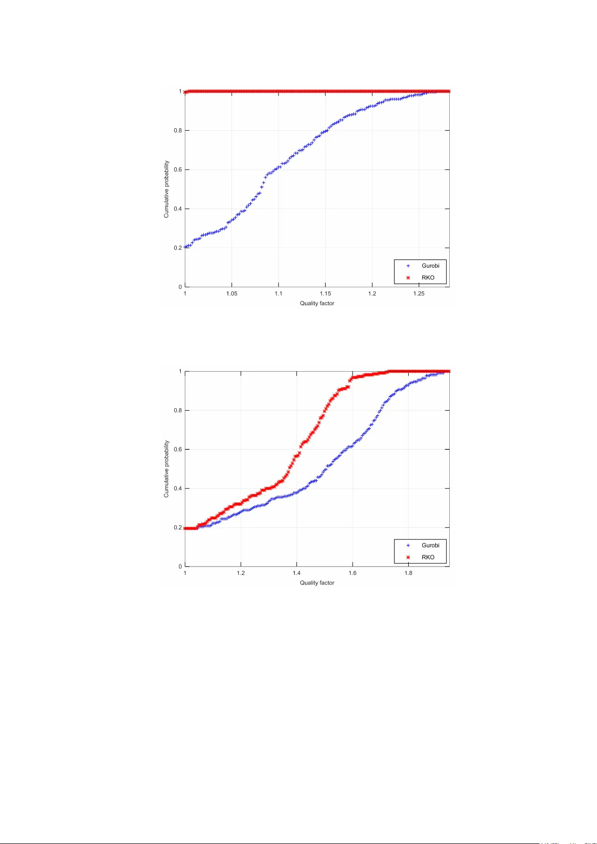
Applying a Random-Key Optimizer on Mixed In teger Programs An tonio A. Cha v es 1* , Mauricio G.C. Resende 1,3 , Carise E. Sc hmidt 2 , J. Kyle Brubak er 4 , Helm ut G. Katzgraber 5 1* F ederal Univ. of S˜ ao P aulo, S. J. dos Camp os, SP , Brazil. 2 Instituto F ederal de San ta Catarina, Chap ec´ o, SC, Brazil. 3 DIMA CS, Piscataw a y, NJ, USA. 4 San Diego, CA, USA. 5 55 North, Cop enhagen, Denmark. *Corresp onding author(s). E-mail(s): an tonio.c hav es@unifesp.br ; Con tributing authors: mgcr@b erk eley .edu ; carise.schmidt@ifsc.edu.br ; j.kylebrubak er@gmail.com ; hgk@55n.vc ; Abstract Mixed-In teger Programs (MIPs) are NP-hard optimization mo dels that arise in a broad range of decision-making applications, including finance, logistics, energy systems, and net work design. Although modern commercial solv ers ha ve ac hieved remark able progress and p erform effectively on many small- and medium-sized instances, their p erformance often degrades when confronted with large-scale or highly constrained formulations. This pap er explores the use of the Random-Key Optimizer (RK O) framework as a flexible, metaheuristic alternativ e for com- puting high-quality solutions to MIPs through the design of problem-sp ecific deco ders. The prop osed approach separates the search process from feasibility enforcemen t by op erating in a contin uous random-k ey space while mapping can- didate solutions to feasible in teger solutions via efficient decoding procedures. W e ev aluate the metho dology on t w o representativ e and structurally distinct b enc hmark problems: the mean–v ariance Marko witz portfolio optimization prob- lem with buy-in and cardinality constrain ts, and the Time-Dep enden t T rav eling Salesman Problem. F or eac h formulation, tailored deco ders are dev elop ed to reduce the effective searc h space, promote feasibilit y , and accelerate conv ergence. Computational exp erimen ts demonstrate that RKO consistently pro duces com- p etitiv e, and in several cases superior, solutions compared to a state-of-the-art commercial MIP solv er, both in terms of solution quality and computational time. 1 These results highlight the potential of RK O as a scalable and v ersatile heuristic framew ork for tac kling challenging large-scale MIPs. Keyw ords: Mixed-In teger Programs, Heuristic, Random-Key , Optimization. 1 In tro duction Mixed In teger Programs (MIPs) are a broad class of NP-hard optimization problems where the goal is to minimize some ob jectiv e sub ject to constraints, with some or all of the v ariables constrained to b e integer-v alued ( Karp , 2009 ; Papadimitriou and Steiglitz , 1982 ). Applications of MIPs can be found in virtually every industry , in areas suc h as transp ortation and logistics, telecommunications, man ufacturing, and finance. Prominen t examples include capacity planning, resource allo cation, bin packing, and p ortfolio optimization, among others ( Korte and Vygen , 2018 ). Commercial black-box solv ers suc h as CPLEX, Gurobi or Xpress are t ypically used to solv e MIPs, leaving end users with potentially costly licensing fees and limited insights in to the anatom y of the underlying algorithms used. Moreo ver, these solvers typically rely on the branch-and- b ound (B&B) paradigm that can solv e small and in termediate-size problems efficiently to optimality , but often suffer from exponential runtimes in the size of the input, calling for the dev elopment of nov el, efficient metho ds that can deal with the ever-increasing scale of real-w orld optimization problems. This w ork sho ws how a broad class of (heuristic) random-k ey optimizers (RK O) ( Cha ves et al. , 2025 ) can be used to solve mixed integer programs. Sp ecifically , w e out- line a general metho d that can lev erage a plethora of optimization paradigms such as genetic algorithms, physics-inspired algorithms (e.g., simulated annealing), or swarm- based algorithms (e.g., particle swarm optimization, or an t colony optimization), all within one unified framework, while (b y design) natively enco ding a large class of con- strain ts such as in tegrality constraints, v ariable bounds, and cardinality constraints of the underlying MIPs. Our approac h is schematically depicted in Figure 1 . Next, w e illustrate our approach with numerical exp erimen ts for tw o b enc hmark problems: the canonical mean-v ariance Mark owitz portfolio optimization problem in the presence of buy-in and cardinalit y constraints ( Chang et al. , 2000 ) and the Time-Dependent T rav eling Salesman Problem (TD-TSP) ( Malandraki and Daskin , 1992 ). The k ey contributions of this study include: • W e dev eloped a contin uous optimization algorithm designed for the efficien t solution of MIPs; • W e created innov ative deco ders that directly maps random-key solutions to the Mark owitz p ortfolio and the TD-TSP mo dels; • Our RK O metho d ac hieves high-qualit y solutions with sup erior computational p erformance compared to a commercial solv er. 2 Fig. 1 : Schematic illustration of our approach. Our framework is based on a dis- tinct separation of problem-indep endent (blue h ypercub e) and problem-dep enden t (deco der) mo dules. The searc h for high-quality solutions is p erformed within the (problem-indep enden t) space of random k eys, as can be implemented with a stack of algorithmic paradigms such as genetic algorithms, simulated annealing, or swarm- based algorithms. The deterministic (problem-dep enden t) decoder maps a given random-k ey vector X ∈ [0 , 1) n to a feasible solution x = de c o der ( X ) within the prob- lem space (as displa yed by black dots). F or mixed integer programs, our decoder design allo ws for an efficien t, native enco ding of a plethora of common constrain ts such as in tegrality constraints, v ariable b ounds, and cardinality constraints. The structure of this pap er is as follows. Section 2 in tro duces the Random-key Optimizers. Section 3 establishes the theoretical framework for MIPs. F ollowing this, section 4 details the enco ding/deco ding sc heme within the Mixed-Integer Limited- Asset Marko witz Mo del and the TD-TSP . Section 5 presents our exp erimen ts and results. Finally , section 6 concludes with a summary of the main con tributions and discusses the implications of this research. 2 Random-k ey Optimizers Our approac h utilizes the concept of random k eys, as prop osed in the Biased Random- Key Genetic Algorithm (BRKGA) ( Gon¸ calv es and Resende , 2011 ). T o establish our notation and terminology , we begin with a brief review of BRKGA and demonstrate ho w this algorithm can b e generalized to alternative solution strategies. A refinement of the RKGA prop osed b y Bean ( 1994 ), BRK GA features a heuristic structure for solving optimization problems. Although most of the w ork in the literature has focused on combinatorial optimization problems, BRK GA has also b een applied to con tinuous optimization problems ( Silv a et al. , 2014 ). BRKGA is based on the idea that an y solution to an optimization problem can b e enco ded as a vector of random keys, i.e., a v ector X where each entry is a real num b er, randomly generated in the in terv al [0 , 1). Such a v ector X , inheren tly defined in the hypercub e [0 , 1) n , is mapp ed to a feasible solution for the combinatorial optimization problem using the deco der. This deterministic algorithm takes a vector of random k eys as input and returns a feasible 3 solution to the optimization problem and the solution’s cost. A p enalt y is added to the cost in case of infeasibility . The BRKGA has been generalized into a general RKO paradigm ( Chav es et al. , 2025 ). Similar to BRK GA, RKO uses a vector of random k eys to encode a solution for a com binatorial optimization problem and emplo ys a deco der to ev aluate solu- tions enco ded by the random-key vector. How ev er, in RKO, the problem-indep enden t searc h in the random-key space is generalized b eyond the genetic algorithm to wards a m uch broader class of metaheuristics, using, e.g., Genetic Algorithm (GA), Sim- ulated Annealing (SA), Greedy Randomized Adaptive Searc h Pro cedure (GRASP), Iterated Lo cal Search (ILS), V ariable Neighborho od Searc h (VNS), P article Sw arm Optimization (PSO), and Large Neighborho o d Search (LNS). The RK O framew ork has been extensively expanded to in tegrate v arious meta- heuristic paradigms. F or instance, PSO algorithms hav e been adapted to work with random-k ey encoding for permutation generation, as presented b y Lin et al. ( 2010 ) and Bewoor et al. ( 2017 , 2018 ). Similarly , Garcia-San tiago et al. ( 2015 ) devised a Har- mon y Search (HS) heuristic that leverages random-key enco ding to effectively tac kle job-shop scheduling problems, ensuring the generation of feasible scheduling solutions through the application of HS op erators to random-k ey enco ded harmonies. Ouaarab et al. ( 2015 ) present the random-key Cuck o o Search algorithm to solv e the trav eling salesman problem, in whic h new solutions are generated via L´ evy fligh ts ( Y ang and Deb , 2009 ). F urther contributions include the work of P essoa and Andrade ( 2018 ), who intro- duced four constructive heuristics for the flowshop sc heduling problem, alongside BRK GA, ILS, and Iterated Greedy Search (IGS) approaches that explore sequence- based neigh b orhoo ds. Similarly , Andrade et al. ( 2019 ) dev elop ed BRK GA and ILS approac hes for machine-dependent scheduling problems, employing a deco der that con- v erts random-k ey v ectors in to sc hedules. This adaptable p erm utation-based decoder w as utilized for T abu Search (TS) and SA implemen tations. Inno v ations like implicit path-relinking (IPR), in tro duced by Andrade et al. ( 2021 ), further extend the RKO’s capabilities by exploring the separation betw een problem and solution spaces through path construction within the unit hypercub e, using the deco der for solution ev aluation. The RK O framework also found application in rob ot motion planning, with Sch uetz et al. ( 2022 ) com bining BRKGA with dual annealing for efficient random-k ey space exploration. This work also formally in tro duced the term “RK O”, resulting in a paten t for the authors ( Sch uetz et al. , 2025 ). More recent ly , RK O implementations based on SA, ILS, and VNS ha ve been deplo yed for the tree hub lo cation problem by Mangussi et al. ( 2023 ). Expanding the metaheuristic p ortfolio, Chav es et al. ( 2024 ) developed a GRASP-based RK O approac h, sho w casing its effectiveness across a div erse range of optimization chal- lenges, including the trav eling salesman problem, Steiner triple cov ering problem, node capacitated graph partitioning problem, and the job sequencing problem with tool switc hing. The general pseudo-co de for RKO is describ ed in Algorithm 1 . It starts by accept- ing as input the instance that needs to b e solv ed and a computation time limit ( run time ). Alternatively , one could use as a stopping rule a maxim um n umber of calls 4 to the decoder ( run dc al ls ). Next, a user-specified set of metaheuristic algorithms is established. Lines 2 and 3 read the instance data and initialize the po ol of solutions at random. Each metaheuristic algorithm runs concurrently in the parallel pro cedure describ ed in lines 4-6, exchanging information through the p o ol of solutions. Finally , the algorithm returns the b est solution from this p o ol. Algorithm 1: Random-Key Optimizer (RKO) Input: instanc e , run time Output: X b est MH ← { MH 1 , MH 2 , . . . , MH m } // Create metaheuristic list ReadD a t a ( instanc e ) // Read instance data Crea tePoolSolutions ( p o ol [ ] , size p o ol ) // Random solution pool while curr entTime ≤ run time do for i ∈ MH in p ar al lel do // Run all MHs in parallel MH ( i ) X b est ← p o ol [0] Sev eral k ey comp onen ts form the foundation of the RKO. It has a p ool of elite solutions that carefully preserves the best and most v aried solutions found during the optimization pro cess, as w ell as a generator of random initial solutions to start the searc h pro cess. F our different mov es are employ ed by a shaking mechanism to p erturb random-k ey vectors, enabling efficient exploration of the solution space. F urthermore, t wo solutions are combined to create a new one using a blending metho d, whic h is an adaptation of uniform crosso ver. Lastly , to direct the search for the b est solutions, the framework uses a v ariet y of metaheuristic algorithms in addition to lo cal searc h heuristics. This method starts with siz e pool solutions and maintains a shared p ool of elite solutions. Any new solution found by a metaheuristic during the search pro cess that outp erforms its curren t best is considered for inclusion in this elite po ol. This inclusion is sub ject to tw o restrictions: the new solution cannot be a cop y of any existing solution in the p o ol, and if it is approv ed, it replaces the solution with a worse ob jectiv e v alue that is most similar to it, ensuring that the p ool’s size remains constan t. T o add con trolled perturbations to a random-k ey v ector, the shaking metho d, whic h is essen tial for div ersification, first chooses a perturbation rate β at random. F our different neigh b orhoo d mo ves are then applied based on this rate. Tw o randomly selected keys, X [ i ] and X [ j ], hav e their v alues switched b y the Swap mov e. A key X [ i ] is swapped with its immediate successor, X [ i + 1], using the Swap Neigh b or mov e. By using the Mirror mo ve, a k ey X [ i ] is swapped out for its complemen t 1 . 0 − X [ i ]. Moreo ver, the Random mo ve ensures a thorough exploration of the solution space by substituting a completely new random v alue for a k ey X [ i ]. The blending metho d combines tw o solutions, χ a and χ b , to create a new random- k ey vector χ c . By incorp orating additional stochastic comp onen ts, this procedure builds up on the concept of Uniform Crossov er (UX) ( Da vis , 1991 ). There is a proba- bilit y ρ of χ c directly inheriting a v alue from either solution χ a or solution χ b for ev ery 5 k ey χ c [ i ]. The contribution from solution χ b is further adjusted by a factor parameter: a factor of 1 uses χ b [ i ], whilst a factor of − 1 uses 1 . 0 − χ b [ i ]. Additionally , to increase the diversit y of the generated solutions, a new random v alue is assigned to a k ey with a probabilit y µ . T o exploit the search process, we utilize Randomized V ariable Neighborho od Descen t (R VND) ( Subramanian et al. , 2010 ), whic h dynamically randomizes the order of applying lo cal searc h heuristics in each iteration. T o ac hieve this, w e developed four problem-independent lo cal search heuristics specifically designed to operate in the random-k ey solution space: Swap LS, Mirror LS, F arey LS, and an Adapted Nelder- Mead LS. Each of these heuristics ev aluates the quality of neighbor solutions using a deco der. Bey ond traditional evolutionary algorithms, the RKO framew ork supports a wide range of metaheuristics designed especially for the random-key solution space. Before using its search metho d, each metaheuristic algorithm in the RK O b egins its searc h with randomly generated solutions. Nine classical metaheuristics are curren tly included in the RK O framew ork. In addition to an Implicit P ath-Relinking mechanism, there are the following: Sim ulated Annealing ( Kirkpatric k et al. , 1983 ), Greedy Ran- domized Adaptive Search Pro cedure ( F eo and Resende , 1995 ), Iterated Lo cal Search ( Louren¸ co et al. , 2003 ), V ariable Neighborho o d Searc h ( Mladenovi ´ c and Hansen , 1997 ), Large Neigh b orhoo d Searc h ( Pisinger and Ropke , 2010 ), Particle Swarm Optimization ( Kennedy and Eb erhart , 1995 ), Genetic Algorithm ( Holland , 1992 ), Biased Random- Key Genetic Algorithm ( Gon¸ calves and Resende , 2011 ), and BRKGA with Clustering Searc h (BRKGA-CS) ( Chav es and Lorena , 202 1 ). Cha ves et al. ( 2025 ) pro vide a detailed explanation of each of these comp onen ts as w ell as the operations of the RK O framework. The RKO framework is publicly a v ailable in the GitHub rep ository 1 , including its C++ source co de and extensiv e do cumen tation, for more accessibility and transparency . 3 Mixed In teger Programs In this section, w e fo cus on the class of linear mixed-in teger programs (MILPs). Applications of MILPs can be found, e.g., in production planning (including job- shop sc heduling), scheduling (e.g., v ehicle scheduling in transportation netw orks), and telecomm unication netw ork design, among others. Generically , MILPs can be formalized in compact form as argmin x { c T x | Ax ≤ b, l ≤ x ≤ u, x ∈ Z p × R n − p } (1) where the cost vector c ∈ R n sp ecifies the ob jectiv e function, the matrix A ∈ R m × n together with the vector b ∈ R m describ es the constraints, the vectors l, u ∈ R n giv e the low er and upp er v ariable b ounds, resp ectively , and I = { 1 , ..., p } ⊆ [ n ] refers to the index set of in teger v ariables. F or p = n , w e recov er an integer linear program (ILP) known to be NP-hard ( Karp , 1972 ). The latter reduces to 0/1 programming if all v ariables are binary . The size of the problem is typically quantified by the num b er of 1 https://gith ub.com/RKO- solv er 6 v ariables n and the num ber of constraints m . While any p oin t x ∈ R n is a (complete) assignmen t, feasible assignments are those that satisfy all the constrain ts sp ecified in Eq. ( 1 ), and an optimal assignment (or solution) refers to a feasible assignment that also minimizes the ob jectiv e ( Boyd and V andenberghe , 2004 ). 3.1 Theoretical F ramew ork W e now sho w how an y random-key algorithm can b e applied to mixed-integer pro- grams, including MILPs. T o this end, w e propose a decoder design that natively accoun ts for in tegrality constrain ts, x ∈ Z p × R n − p , as well as v ariable bounds, l ≤ x ≤ u . Sp ecifically , for any random key X i ∈ [0 , 1] w e simply take x i = ( in t[ l i − 0 . 5 + ( u i − l i + 1) X i ] , if i ∈ I ; l i + ( u i − l i ) X i , otherwise, with int [ · ] rounding to the closest integer. This mapping yields an integer (b ounded) decision v ariable x i ∈ { l i , l i + 1 , ..., u i } for i ∈ I , and a con tinuous (b ounded) decision v ariable x i ∈ [ l i , u i ], as desired. F or violations of the remaining constrain ts, Ax ≤ b , w e introduce prohibitively large p enalit y v alues, allo wing the algorithm to iteratively steer aw a y from these lo w-fitness solutions ov er the course of the ev olution. Because w e are not b ound to differen tiable loss functions, w e can handle these cases with a simple if-else logic. Sp ecifically , we set ∆ = b − Ax , with ∆ i ≥ 0 indicating satisfied constrain ts and ∆ i < 0 signaling violations thereof. F or any ∆ i < 0 we then add some p enalt y ϕ (∆ i ) to the cost (fitness) v alue f ( x ) as f ( x ) = c T x + m X i =1 ϕ (∆ i ) 1 ∆ i < 0 (2) with indicator function 1 x . The cost v alue f ( x ) provides feedback to the optimizer, and is used to steer the optimizer tow ards feasible assignmen ts o ver the course of the search pro cess. As a simple mo del for the p enalt y function ϕ ( · ) we can take ϕ (∆ i ) = P · ∆ 2 i with pre-factor P > 0, but other models suc h as logistic barrier functions (as used in the context of interior-point metho ds ( Boyd and V andenberghe , 2004 )) may b e used as w ell. The n umerical v alue for the penalty parameter P can b e optimized in an outer lo op. Overall, the proposed deco der design is summarized in pseudo-code in Algorithm 2 . In Section 4 , w e discuss additional decoder designs that address common cardinalit y constrain ts, sub-route elimination, integralit y constraints, and v ariable b ounds. 4 Applications In this pap er, we present tw o case studies of RKO applications for solving MIPs, namely the Mixed-In teger Limited-Asset Marko witz Mo del and the Mixed-Integer TD- TSP Model. Representing the random-keys v ector for these mo dels can include all decision v ariables. Ho w ever, this will increase execution time and unnecessarily restrict con vergence. Therefore, in these approac hes, w e dev elop deco ders that find v alues only for non-zero decision v ariables. 7 Algorithm 2: Example deco der for generic MIPs Input: c, A, b, l, u, p, X Output: x, c ost // Initialize assignment x ← np.zeros(length( X )) // Get integer assignments for i ← 1 to p do x [ i ] ← in t( l [ i ] − 0 . 5 + ( u [ i ] − l [ i ] + 1) · X [ i ]) // Get continuous assignments for i ← p + 1 to length ( x ) do x [ i ] ← l [ i ] + ( u [ i ] − l [ i ]) · X [ i ] // Initialize cost of assignment f ( x ) cost ← c T x // Add penalties for constraint violations ∆ ← b − Ax for ∆ i ∈ ∆ do if ∆ i < 0 then c ost ← c ost + ϕ (∆ i ) 4.1 Mixed-In teger Limited-Asset Mark owitz Model First, to illustrate our approac h, w e consider the canonical Marko witz (mean-v ariance) approac h to p ortfolio selection in the presence of cardinalit y constrain ts that limit a p ortfolio to hav e a sp ecific num ber of assets and bounds on the prop ortion of the p ortfolio held in a giv en asset (if any of the asset is held) ( Chang et al. , 2000 ; Cesarone et al. , 2011 ) as to limit risk exp osure and transaction costs for small inv estmen ts through upp er and low er b ounds, resp ectiv ely . This example sho ws that our approach is not limited to MILPs but can handle non-linear MIPs within the same framework. Let n b e the total n umber of assets av ailable, µ i b e the expected return of asset i ∈ { 1 , ..., n } , Σ ij b e the cov ariance b etw een assets i ∈ { 1 , ..., n } and j ∈ { 1 , ..., n } , and λ b e the risk-av ersion parameter, whic h controls ho w muc h an inv estor p enalizes v ariance relative to expected return, where 0 ≤ λ ≤ 1. F urthermore, let K b e the desired num b er of assets in the p ortfolio, l i b e the minim um prop ortion that m ust b e held of asset i = { 1 , ..., n } (if an y of asset i is held), u i b e the maximum prop ortion that can b e held of asset i = { 1 , ..., n } (if an y of asset i is held), with 0 ≤ l i ≤ u i ≤ 1. In practice, the low er b ounds l i represen t a min-buy or minimum transaction level for asset i , while the upper b ounds u i limit the exp osure of the p ortfolio to individual assets. The decision v ariables are the allo cation w eights w i for asset i ∈ { 1 , ..., n } , with 0 ≤ w i ≤ 1, together with the binary indicator v ariables z i ∈ { 0 , 1 } , with z i = 1, if asset i is held, and z i = 0 otherwise. W e then consider the following mixed-integer optimization problem: min w H ( w ) = λ w ⊤ Σ w − (1 − λ ) µ ⊤ w (3) 8 s.a. n X i =1 w i = 1 , (4) n X i =1 z i = K, (5) l i z i ≤ w i ≤ u i z i , i = 1 , . . . , n, (6) z i ∈ { 0 , 1 } , i = 1 , . . . , n. (7) In the limiting case where λ = 0, we aim to maximize exp ected return (irresp ectiv e of the risk inv olved), and the optimal solution will in volv e a single asset with the highest return. Conv ersely , for λ = 1 our goal is to minimize risk (irresp ectiv e of the return inv olv ed), and the optimal solution will t ypically in v olve a larger num b er of assets. In termediate v alues with 0 < λ < 1 describ e an explicit trade-off b et w een risk and return. F or example, for λ = 0 . 25 the ob jectiv e b ecomes 0 . 25[ r isk ] − 0 . 75[ r eturn ]. This problem features four (families of ) constraints. Constraint ( 4 ) represen ts the budget constrain t, given that the a v ailable funds are limited. Constraint ( 5 ) refers to the cardinality constraint, forcing us to select the b est p ortfolio with inv estments in exactly K assets. Note that we hav e explicitly chosen to formulate this problem with an equality (rather than an inequalit y) with resp ect to the n umber of assets K in the p ortfolio. This is b ecause if we can solv e the equality-constrained case (as considered here), then an y situation inv olving inequalities (lo wer or upp er limits on the num b er of assets in the p ortfolio) can b e solved in a series of equiv alent problems (that are trivially parallelized). Sp ecifically , the generalized constraint K L ≤ Σ i z i ≤ K U can b e dealt with by simply studying all v alid v alues of K , i.e., K = { K L , K L + 1 , ..., K U } ( Chang et al. , 2000 ). Constraints ( 6 ) describ e the v ariable b ounds, requiring that all non-zero in vestmen ts lie within the inv estment band describ ed by lo wer l and upp er b ounds u , respectively . These constrain ts couple the in teger v ariables z i with the con tinuous v ariables w i . Finally , constraints ( 7 ) imp ose integralit y on the v ariables z i , making them binary indicator v ariables. 4.1.1 Enco ding/Deco ding W e now illustrate the simplicity and flexibilit y of our approach, with one deco der design for the non-linear MIP describ ed in Eq. ( 3 )–( 7 ). This deco der handles integralit y constrain ts ( z i ∈ { 0 , 1 } ), budget, and cardinality constraints nativ ely b y design, mean- ing that these constraints will alw ays b e fulfilled automatically b y the deco der. The remaining v ariable bounds constrain ts are accounted for via soft p enalt y terms that effectiv ely fold violations of these constraints in to the cost function, thereb y steering the solv er tow ards feasible (low-cost) solutions throughout the search pro cess. Eac h solution corresp onds to a random-key v ector of size 2 × K , with each random k ey represen ting a real v alue in the interv al [0 , 1). The decoder maps eac h solution in to a set of selected assets and conti nuous w eights. The first K random keys are 9 con verted into an iden tifier corresponding to one of the a v ailable assets (an in te- ger num ber b elonging to the set { 1 , ..., n } ), while the second blo c k represents the con tinuous weigh ts. See an example of this enco ding in Figure 2 . W e first create a list of size n containing all av ailable assets en umerated b y an iden- tifier 1 , ..., n . This deco der is applied iteratively and without replacement by selecting an asset in eac h of K iterations. Initially , the first random key is m ultiplied by n and the ceiling function is applied. This integer num b er obtained corresp onds to the first selected asset’s identifier ( id ), giving z id = 1. This asset will b e remov ed from the list for subsequent iterations. Thus, the set of assets to b e considered in the next iteration has a size n − 1. Next, the second selected asset is selected from the second random k ey , m ultiplied by n − 1, and the ceiling function is applied. This num b er corresp onds to the iden tifier of the second selected asset. This pro cess is rep eated un til K assets are selected. After selecting the i -th asset, the contin uous w eight of the asset id is set by a simple affine transformation using the random key i + K , w id = l i + ( u i − l i ) × X [ i + K ]. Finally , a simple p ost-processing step alw ays satisfies the budget constrain t with the transformation w i = w i / P n i =1 w i . How ev er, this transformation ma y violate the v ariable b ound constraints, which can b e handled with a simple p enalty term prop or- tional to the extent to whic h each v ariable w i violates its low er and upp er bounds. A fixed p enalt y is also added to av oid ov erly small p enalties. Algorithm 3 illustrates the pseudo code of the deco der, and Figure 2 presen ts an example of mapping the random- k ey v ector X = { 0 . 81 , 0 . 32 , 0 . 54 , 0 . 25 , 0 . 15 , 0 . 91 } of size K = 3 for a dataset with n = 10 assets. Algorithm 3: Deco der for p ortfolio optimization problem Input: µ, Σ , λ, l, u, K, X Output: w , z , cost assets ← { 1 , ..., n } for i ← 1 to K do id ← assets [ceiling( X [ i ] × ( n + 1 − i )] z [ id ] ← 1 w [ id ] ← l [ id ] + ( u [ id ] − l [ id ]) × X [ i + K ] assets ← assets \ id for i ← 1 to n do w [ i ] ← w [ i ] / P i w i p enalty ← max(0 , w [ i ] − u i ) + max(0 , l i − w [ i ]) cost ← λ w ⊤ Σ w − (1 − λ ) µ ⊤ w + (10 4 × p enalty + 10 3 × 1 { p enalty > 0 } ) 4.2 Mixed-In teger TD-TSP Mo del As a second example, w e fo cus on the TD-TSP , in whic h v ariations in trav el times o ver the planning horizon are explicitly tak en into account in the routing decisions. A single v ehicle lea ves a dep ot, serves each customer exactly once, and returns to the dep ot, where the time needed to tra vel from one lo cation to the next dep ends on the 10 K = 3 n = 10 l i = 0 . 01 u i = 0 . 40 1 2 3 4 5 6 0.81 0.32 0.54 0.29 0.15 0.91 iter 1 i = 1 assets = { 1 , 2 , 3 , 4 , 5 , 6 , 7 , 8 , 9 , 10 } id = assets [ ceiling (0 . 81 × 10)] = as sets [9] = 9 z [9] = 1 w [9] = 0 . 01 + (0 . 40 − 0 . 01) × 0 . 29 = 0 . 1231 iter 2 i = 2 assets = { 1 , 2 , 3 , 4 , 5 , 6 , 7 , 8 , 10 } id = assets [ ceiling (0 . 32 × 9)] = as sets [3] = 3 z [3] = 1 w [3] = 0 . 01 + (0 . 40 − 0 . 01) × 0 . 15 = 0 . 0685 iter 3 i = 3 assets = { 1 , 2 , 4 , 5 , 6 , 7 , 8 , 10 } id = assets [ ceiling (0 . 54 × 8)] = as sets [5] = 6 z [6] = 1 w [6] = 0 . 01 + (0 . 40 − 0 . 01) × 0 . 91 = 0 . 3649 sumW = 0 . 1231 + 0 . 0685 + 0 . 3649 = 0 . 5565 w [9] = 0 . 1231 / 0 . 5565 = 0 . 2212 , penalty = 0 w [3] = 0 . 0685 / 0 . 5565 = 0 . 1231 , penalty = 0 w [6] = 0 . 3649 / 0 . 5565 = 0 . 6557 , penalty = 0 . 2557 Cost = λ risk − (1 − λ ) r eturn +  10 4 × penalty + 10 3 × 1 { penalty> 0 }  Fig. 2 : Deco ding example. The selected assets are 9, 3, and 6. departure time and is mo deled b y discretizing the planning horizon into time in terv als. This setting captures v ariations in trav el conditions, suc h as recurrent congestion patterns, and leads to a time-indexed MILP form ulation in which routing and timing decisions are tigh tly integrated. Let G = ( V , A ) b e a directed graph, where V = { 0 , 1 , 2 , ..., n, n + 1 } denotes the set of no des and A = { ( i, j ) ∈ V × V : i  = j } \ { (0 , n + 1) , ( n + 1 , 0) } denotes the set of arcs. No de 0 represents the dep ot, while n + 1 is a dumm y no de, i.e., a copy of the dep ot used to mark the end of the route. Let V c denote the subset of customers that must b e served, i.e., V c = V \ { 0 , n + 1 } . Each customer i ∈ V c has an asso ciated deterministic service time s i > 0; b y conv en tion, we set s 0 = s n +1 = 0. The graph G is time-dependent, meaning that as traffic conditions c hange, the tra vel time on each arc ( i, j ) ∈ A can v ary . The planning horizon is discretized into a set H = { 0 , 1 , 2 , ..., m } of m + 1 time interv als of equal length ¯ T . F or each time interv al h ∈ H , traffic conditions are assumed to b e constant ov er [ h ¯ T , ( h + 1) ¯ T ). Accordingly , for every arc ( i, j ) ∈ A and time in terv al h ∈ H let t h ij denote the deterministic trav el time required to trav erse arc ( i, j ) ∈ A when departure tak es place in in terv al h ∈ H . W e use a form ulation with a time-discretized representation of trav el times ( Malan- draki and Daskin , 1992 ), embedded in a tw o-commo dit y flow mo del on an exte nded net work ( Baldacci et al. , 2003 , 2004 ), and define the following decision v ariables. Let x h ij denote binary v ariables that take v alue 1 if arc ( i, j ) ∈ A is trav ersed in time inter- v al h ∈ H , and 0 otherwise. Let y ij denote contin uous nonnegative flow v ariables that supp ort a tw o-commo dit y flow represen tation of the route: whenev er arc ( i, j ) ∈ A b elongs to the route, y ij represen ts the flow asso ciated with customers that still need to b e serv ed, whereas y j i represen ts the flow associated with customers that ha v e already b een served. Finally , let a i denote con tinuous nonnegative v ariables represen ting the accum ulated time up on departure from node i ∈ V \ { n + 1 } or up on arriv al at the 11 terminal node n + 1. W e consider the follo wing mixed-integer optimization problem: M in X ( i,j ) ∈ A X h ∈ H x h ij t h ij (8) s.a. x h i 0 = 0 , ∀ i ∈ V c , ∀ h ∈ H, (9) x h ( n +1) j = 0 , ∀ j ∈ V c , ∀ h ∈ H, (10) X j ∈ V c x 0 0 j = 1 , (11) X j ∈ V c X h ∈ H \{ 0 } x h 0 j = 0 , (12) X j ∈ V \{ 0 ,i } X h ∈ H x h ij = 1 , ∀ i ∈ V c , (13) X i ∈ V \{ j,n +1 } X h ∈ H x h ij = 1 , ∀ j ∈ V c , (14) X i ∈ V c X h ∈ H x h i ( n +1) = 1 , (15) X j ∈ V \{ i } ( y j i − y ij ) = 2 , ∀ i ∈ V c , (16) X j ∈ V c y 0 j = n, (17) X i ∈ V c y i 0 = 0 , (18) X j ∈ V c y ( n +1) j = n, (19) y ij + y j i = n X h ∈ H ( x h ij + x h j i ) , ∀ ( i, j ) ∈ A, i < j, (20) a 0 = 0 , (21) a i + s j + t h ij − 2 ¯ T | H | (1 − x h ij ) ≤ a j (22) a j ≤ a i + s j + t h ij + ¯ T | H | (1 − x h ij ) , ∀ ( i, j ) ∈ A, ∀ h ∈ H . X j ∈ V \{ 0 } X h ∈ H ¯ T hx h ij ≤ a i < X j ∈ V \{ 0 } X h ∈ H ¯ T ( h + 1) x h ij , ∀ i ∈ V c , (23) a n +1 < ¯ T | H | , (24) x h ij ∈ { 0 , 1 } , ∀ ( i, j ) ∈ A, ∀ h ∈ H , (25) y ij ≥ 0 , ∀ ( i, j ) ∈ A, (26) a i ≥ 0 , ∀ i ∈ V . (27) 12 The ob jectiv e function ( 8 ) minimizes the total tra vel time of the route. Constrain ts ( 9 )–( 10 ) ensure that no arc en ters the depot and no arc lea ves the terminal, so that an y feasible solution is a directed path from the dep ot to the terminal. The departure from the dep ot is forced to o ccur in the first time interv al h ∈ H by constraints ( 11 )–( 12 ). The assignmen t constraints ( 13 )–( 15 ) then guarantee that the route starts at the depot, serves each customer exactly once, and ends at the terminal. Balance constrain ts ( 16 ) at the customer no des ensure the conserv ation of the flo w asso ciated with customers that hav e already b een served and those that still need to b e served. Constrain ts ( 17 )–( 19 ) define the corres ponding b oundary conditions at the dep ot and at the terminal, while constraints ( 20 ) link the routing and flo w v ariables, enforce connectivit y of the solution, and eliminate subtours. The departure time from the dep ot at the b eginning of the first time interv al is fixed by constraint ( 21 ). Departure times at the no des are con trolled by constraints ( 22 ) along the route within the time- discretized framew ork, while constraints ( 23 )–( 24 ) iden tify , for each no de, the time in terv al in which tra versing starts and ensure that the route is completed within the planning horizon. Finally , constraints ( 25 )–( 27 ) sp ecify the domains of the decision v ariables. In addition, w e include the v alid inequality ( 28 ), where L denotes a low er b ound on the total tra vel time of any feasible route. The constan t L is defined as the sum of the smallest trav el times lea ving each eligible no de o ver all time interv als, namely , L = min j ∈ V c t 0 0 j + P i ∈ V c min j ∈ V \{ 0 ,i } h ∈ H t h ij . V alid inequalit y ( 28 ) X ( i,j ) ∈ A X h ∈ H x h ij ≥ L. (28) is used to further tighten the formulation. 4.2.1 Enco ding/Deco ding W e now illustrate ho w our approac h applies to the TD-TSP by designing a deco der for the MILP in ( 8 )–( 27 ). The deco der enforces integralit y and routing constraints by construction: it alw ays generates a simple route that departs from the depot, serv es eac h customer exactly once, and ends at the terminal node n + 1 (a cop y of the depot), so that degree and connectivity requirements are automatically satisfied. The time- dep enden t structure and the planning horizon are handled by sim ulating the route o ver time, with trav el times ev aluated as a function of the current departure time and the corresp onding time interv al up dated at each step. Whenever the accumulated time exceeds the planning horizon, a large p enalty is added to the ob jective v alue, discouraging such solutions and guiding the search to ward routes that resp ect the discretized planning horizon. Eac h solution is encoded as a random-k ey vector of length n , where n is the num ber of customers and each key is a real v alue in [0 , 1). The deco der maps this v ector into a permutation v = ( v 1 , . . . , v n ) of V c b y sorting the customers in nondecreasing order of their random-key v alues. This permutation defines ho w the v ariables x h ij are set, 13 with the dep ot fixed as the starting no de 0 and its cop y (the terminal no de n + 1) designated as the end of the route. An illustrative example is giv en next. Giv en the p ermutation v = ( v 1 , . . . , v n ), the deco der ev aluates the time-dep enden t cost b y sim ulating the route o ver the discretized planning horizon. The vehicle departs from the depot at time zero and tra v erses the arc sequence (0 , v 1 ) , ( v 1 , v 2 ) , . . . , ( v n , n + 1), up dating the accum ulated time and the corresp onding departure in terv al h ∈ H after eac h mov e. Initially , the curren t no de, c , is the starting no de 0 and i = v 1 , then the v ariable x h c,v i is set as 1. The curren t customer c is up dated to v i , the next customer in the sequence v is set to v i , and the process is repeated. While the accum ulated time remains within the planning horizon, the deco der accum ulates the corresp onding time-dep enden t tra vel and service times; once the horizon is exceeded, the visiting order is fixed, and the solution is p enalized. F rom the MILP p ersp ectiv e, the simulation induces a sparse v ariable assignmen t. F or eac h arc ( i, j ) on the deco ded route, the deco der sets x h ij = 1 for h =  a i / ¯ T  and sets all other x -v ariables to zero. The flo w v ariables follow the same incidence pattern: if arc ( i, j ) is not used, ( y ij , y j i ) = (0 , 0); otherwise, ( y ij , y j i ) is assigned to satisfy the flo w-balance constraints and ( 20 ), implying y ij + y j i = n for each selected pair { i, j } . T ogether with the sim ulated departure times a i , this defines a complete MILP-consisten t assignment of the routing, flow, and timing v ariables for the deco ded route. As in the portfolio optimization example, the random-key representation fo cuses on the core combinatorial structure of the solution. Here, the random-key vector enco des only the visiting order of the customers, rather than the full set of time-indexed deci- sion v ariables in the MILP formulation. This substantially reduces the dimensionality of the search space, whic h is b eneficial for the efficiency of the search pro cedure. In turn, the decoder is resp onsible for enforcing the routing constraints and for accurately ev aluating the time-dependent trav el cost and feasibilit y of each candidate solution. Algorithm 4 summarizes the deco der pseudo code, and Figure 3 presents an example of mapping a random-k ey vector X = { 0 . 81 , 0 . 32 , 0 . 54 , 0 . 25 , 0 . 15 , 0 . 91 } for a dataset with n = 6 customers. 5 Exp erimen ts and Results This section demonstrates the feasibility and performance of the random-k ey approac h using n umerical tests on tw o sets of benchmark instances. The first set consists of pub- licly av ailable b enc hmark instances 2 based on real-world data for the limited asset, or cardinalit y-constrained, Marko witz. The instances comprise expected return v ectors and cov ariance matrices of sizes b etw een 31 and 2151 constructed from weakly priced data for Hang Seng (31 assets), DAX (85 assets), FTSE (89 assets), S&P (98 assets), Nikk ei (225 assets), S&P 500 (457 assets), Russell 2000 (1318 assets) and Russell 3000 (2151 assets). Each instance w as tested with different v alues of K to analyze the influ- ence of this parameter on the optimization metho ds. The parameters l i and u i w ere 2 OR-Library: h ttps://www.brunel.ac.uk/ ∼ mastjjb/jeb/info.html 14 Algorithm 4: Deco der for the TD-TSP Input: n, | H | , ¯ T , s [ i ] , ∀ i ∈ V , t [ i ][ j ][ h ] , ∀ ( i, j ) ∈ A, ∀ h ∈ H , X Output: x, y, a, cost v ← [1 , ...n ] Sort v [1 , ..., n ] in nondecreasing order of X [ v [ i ]] penality ← 0; cost ← 0; h ← 0; curr ent ← 0; f low ← n ; a [0] ← 0 for i ← 1 to n do if h < | H | then x [ curr ent ][ v [ i ]][ h ] ← 1 a [ v [ i ]] ← a [ cur rent ] + t [ cur rent ][ v [ i ]][ h ] + s [ v [ i ]] h ←  a [ v [ i ]] / ¯ T  else x [ curr ent ][ v [ i ]][ | H | − 1] ← 1 a [ v [ i ]] ← a [ cur rent ] + t [ cur rent ][ v [ i ]][ | H | − 1] + s [ v [ i ]] y [ cur rent ][ v [ i ]] ← f l ow y [ v [ i ]][ curr ent ] ← n − f low f low ← f low − 1 curr ent ← v [ i ] if ( h < | H | ) ∧ (( a [ curr ent ] + t [ cur rent ][0][ h ]) < | H | ¯ T ) then x [ curr ent ][ n + 1][ h ] ← 1 a [ n + 1] = a [ curr ent ] + t [ cur rent ][0][ h ] else x [ curr ent ][ n + 1][ | H | − 1] ← 1 a [ n + 1] ← a [ cur rent ] + t [ cur rent ][0][ | H | − 1] penality ← 10 3 y [ cur rent ][ n + 1] ← f low y [ n + 1][ cur rent ] ← n − f low cost ← P ( i,j ) ∈ A P h ∈ H t h ij x h ij + | H | ¯ T × penality n = 6; | H | = 2; ¯ T = 30 1 2 3 4 5 6 0.81 0.32 0.54 0.29 0.15 0.91 5 4 2 3 1 6 0.15 0.29 0.32 0.54 0.81 0.91 s 1 s 2 s 3 s 4 s 5 s 6 5 5 6 4 3 4 h = 0 0 1 2 3 4 5 6 7 0 0 5 7 4 1 3 6 0 1 4 0 8 1 1 4 2 4 2 7 8 0 5 2 6 6 7 3 5 2 4 0 1 3 2 5 4 3 1 2 1 0 7 8 3 5 2 3 5 3 9 0 4 2 6 5 2 8 2 7 2 0 5 7 0 5 7 4 1 3 6 0 h = 1 0 1 2 3 4 5 6 7 0 0 8 10 3 1 2 4 0 1 7 0 8 1 3 4 4 7 2 9 8 0 6 2 6 8 9 3 5 4 4 0 1 3 6 5 4 2 1 2 1 0 7 8 2 5 3 2 5 4 11 0 4 3 6 5 3 8 7 7 2 0 5 7 0 8 10 3 1 2 4 0 a [0] = 0; h = 0; penalty = 0; x [0][5][0] = 1; y [0][5] = 6; y [5][0] = 0; a [5] = a [0] + t [0][5][0] + s [5] = 0 + 3 + 3 = 6; h = 0; penalty = 0; x [5][4][0] = 1; y [5][4] = 5; y [4][5] = 1; a [4] = a [5] + t [5][4][0] + s [4] = 6 + 9 + 4 = 19; h = 0; penalty = 0; x [4][2][0] = 1; y [4][2] = 4; y [2][4] = 2; a [2] = a [4] + t [4][2][0] + s [2] = 19 + 2 + 5 = 26; h = 0; penalty = 0; x [2][3][0] = 1; y [2][3] = 3; y [3][2] = 3; a [3] = a [2] + t [2][3][0] + s [3] = 26 + 5 + 6 = 37; h = 1; penalty = 0; x [3][1][1] = 1; y [3][1] = 2; y [1][3] = 4; a [1] = a [3] + t [3][1][1] + s [1] = 37 + 4 + 5 = 46; h = 1; penalty = 0; x [1][6][1] = 1; y [1][6] = 1; y [6][1] = 5; a [6] = a [1] + t [1][6][1] + s [6] = 46 + 4 + 4 = 54; h = 1; penalty = 0; x [6][7][1] = 1; y [6][7] = 0; y [7][6] = 6; a [7] = a [6] + t [6][7][1] = 54 + 5 = 59; h = 1; penalty = 0; Cost = P ( i,j ) ∈ A P h ∈ H t h ij x h ij + | H | ¯ T × penal ty Fig. 3 : Deco ding example. The selected customer visiting sequence 5 − 4 − 2 − 3 − 1 − 6. 15 fixed at 0.01 and 0.25, resp ectiv ely . F or the first set of exp erimen ts, the mathemati- cal mo del ( 3 )-( 7 ) w as solved using Gurobi v ersion 12.0.2 ( Gurobi Optimization , 2024 ) with a time limit of 1800s. F or the TD-TSP experiments, we consider a second set of 225 instances deriv ed from real traffic data. This set co vers problems with n ∈ { 10 , 12 , 14 , 20 , 22 , 24 , 50 , 52 , 54 , 80 , 82 , 84 , 100 , 102 , 104 } customers. Eac h customer i ∈ V c is asso ciated with a deterministic service time s i whose v alue lies in an in terv al [ m, M ] that depends on the size of the instance: s i ∈ [1800 , 2700]s for n ∈ { 10 , 12 , 14 } , s i ∈ [900 , 1500] for n ∈ { 20 , 22 , 24 } , s i ∈ [360 , 600] for n ∈ { 50 , 52 , 54 } , s i ∈ [180 , 360] for n ∈ { 80 , 82 , 84 } and s i ∈ [120 , 240] for n ∈ { 100 , 102 , 104 } . The planning horizon is fixed at 54,000s and is discretized into | H | ∈ { 5 , 10 , 15 } time interv als of equal length. F or eac h instance size n we therefore consider three time- discretization schemes, one for each v alue of | H | . F or every combination of instance size n and n umber of time interv als | H | , fiv e indep enden t instances are defined, leading to a total of 225 test instances. F or this exp erimen t, the mathematical model ( 8 )–( 27 ), with the v alid inequality ( 28 ), was solved using Gurobi version 12.0.2 ( Gurobi Optimization , 2024 ) with a time limit of 1800s. In all TD-TSP exp erimen ts, Gurobi w as provided with an initial incumbent solution obtained from a greedy heuristic. The RKO framework w as co ded in C++ and compiled using GCC. The RKO framew ork is av ailable at https://gith ub.com/RK O- solver . All exp eriments were con- ducted on a PC with a Dual Xenon Silv er 4114 20c/40t 2.2GHz pro cessor, 96GB of DDR4 RAM, and Ubuntu 24.04.2 x64. 5.1 Computational Results for the Limited Asset Mark owitiz The RKO was run 30 times for eac h instance, with different seeds and a CPU time restriction ( run time ). The CPU time limit for the RK O was set in seconds. A step func- tion run time ( n ) was constructed to transfer the n umber of assets to discrete run time lev els. The runtime is defined as r un time ( n ) = v for n in the resp ectiv e interv als, where the pairs ( v , interv al) are: (10 , n ≤ 31), (20 , 31 < n ≤ 98), (30 , 98 < n ≤ 225), (50 , 225 < n ≤ 457), (100 , 457 < n ≤ 1318), and (200 , n > 1318). T ables 1 – 3 show the computational results of Gurobi and RKO to solve the p ortfolio selection problem with three differen t v alues of λ = { 0 . 3 , 0 . 5 , 0 . 7 } . These tables con tain information ab out the instances ( n , K , l i , u i , and λ ), the results of Gurobi (upp er b ound (UB), lo wer b ound (LB), gap(%), and the total time to find the optimal solution - limited to 1800s), and the results of RKO (ob jective function of the b est solution found in 30 runs (OFV), relativ e p ercentage deviation (RPD), and the av erage computational time to find the b est solution). W e calculated the RPD = (OFV / UB − 1) × 100, which considers the ob jectiv e function v alue of the b est solutions found b y RKO and the upp er b ound of Gurobi. W e calculated tw o metrics: first, in terms of the b est solution found in 30 runs (RPD b ) and second, as an av erage of the RPD found in each of the 30 runs (RPD a ). Lo oking at the tables, we note that Gurobi solved up to the Nikkei instance in a few seconds. Ho wev er, starting with the S&P 500 instances, Gurobi solved only one instance within the 1800-second limit (S&P 500 with K = 20 and λ = 0 . 3). As the v alue of λ increases, the gaps b et w een instances b ecome larger. This b eha vior sho ws 16 T able 1 : Computational results ( λ = 0 . 3). Gurobi RKO Instance n K l i u i λ UB LB gap(%) total time (s) OFV RPD b RPD a best found at (s) port1 (Hang Seng) 31 5 0.01 0.25 0.3 -0.00466 -0.00466 0.00 0.02 -0.00466 0.00 0.01 6.64 8 -0.00465 -0.00465 0.00 0.01 -0.00465 0.00 0.00 9.77 10 -0.00464 -0.00464 0.00 0.01 -0.00464 0.01 0.01 9.94 15 -0.00461 -0.00461 0.00 0.01 -0.00461 0.03 0.10 9.97 port2 (DAX) 85 10 0.01 0.25 0.3 -0.00532 -0.00532 0.00 0.03 -0.00532 0.00 0.05 19.89 20 -0.00515 -0.00515 0.00 0.03 -0.00515 0.12 0.17 19.95 25 -0.00505 -0.00505 0.00 0.03 -0.00504 0.29 0.38 20.00 45 -0.00435 -0.00435 0.00 0.03 -0.00421 3.20 3.30 19.98 port3 (FTSE) 89 10 0.01 0.25 0.3 -0.00448 -0.00448 0.00 0.03 -0.00448 0.02 0.02 19.47 20 -0.00439 -0.00439 0.00 0.03 -0.00439 0.04 0.10 19.85 25 -0.00432 -0.00432 0.00 0.03 -0.00432 0.05 0.10 19.95 45 -0.00388 -0.00388 0.00 0.03 -0.00359 7.71 7.96 20.00 port4 (S&P) 98 10 0.01 0.25 0.3 -0.00549 -0.00549 0.00 0.04 -0.00549 0.00 0.01 19.78 20 -0.00531 -0.00531 0.00 0.04 -0.00531 0.04 0.15 19.95 30 -0.00507 -0.00507 0.00 0.04 -0.00505 0.40 0.53 19.99 50 -0.00440 -0.00440 0.00 0.04 -0.00407 7.48 7.52 19.99 port5 (Nikkei) 225 10 0.01 0.25 0.3 -0.00230 -0.00230 0.00 0.12 -0.00230 0.02 0.02 28.45 20 -0.00219 -0.00219 0.00 0.12 -0.00219 0.03 0.51 29.95 30 -0.00202 -0.00202 0.00 0.12 -0.00198 2.40 3.54 29.96 50 -0.00158 -0.00158 0.00 0.12 -0.00143 9.51 10.81 29.92 port6 (S&P 500) 457 20 0.01 0.25 0.3 -0.00888 -0.00888 0.00 338.80 -0.00888 0.03 0.04 49.94 40 -0.00836 -0.00839 0.40 1800.99 -0.00815 2.46 2.74 49.84 50 -0.00799 -0.00807 1.00 1800.63 -0.00749 6.29 7.48 49.92 70 -0.00711 -0.00729 2.48 1800.99 -0.00651 8.46 10.58 49.94 port7 (Russell 2000) 1318 30 0.01 0.25 0.3 -0.01226 -0.01239 1.05 1808.74 -0.01224 0.16 0.38 99.87 50 -0.01165 -0.01190 2.14 1812.12 -0.01151 1.24 1.41 99.98 60 -0.01126 -0.01157 2.76 1813.51 -0.01115 0.99 1.07 99.96 80 -0.01034 -0.01080 4.48 1805.09 -0.01019 1.44 2.95 99.51 port8 (Russell 3000) 2151 40 0.01 0.25 0.3 -0.00725 -0.00732 0.86 1814.92 -0.00709 2.27 2.31 199.67 60 -0.00624 -0.00689 10.49 1810.55 -0.00643 -3.11 -2.79 199.86 70 -0.00588 -0.00669 13.78 1810.11 -0.00616 -4.63 -4.26 199.96 90 -0.00534 -0.00609 14.00 1810.22 -0.00542 -1.49 -1.04 199.86 T able 2 : Computational results ( λ = 0 . 5). Gurobi RKO Instance n K l i u i λ UB LB gap(%) total time (s) OFV RPD b RPD a best found at (s) port1 (Hang Seng) 31 5 0.01 0.25 0.5 -0.00297 -0.00297 0.00 0.43 -0.00297 0.00 0.00 8.36 8 -0.00297 -0.00297 0.00 0.03 -0.00297 0.02 0.02 9.93 10 -0.00296 -0.00296 0.00 0.01 -0.00296 0.00 0.01 9.91 15 -0.00293 -0.00293 0.00 0.01 -0.00293 0.08 0.15 9.98 port2 (DAX) 85 10 0.01 0.25 0.5 -0.00365 -0.00365 0.00 0.03 -0.00365 0.00 0.03 19.22 20 -0.00354 -0.00354 0.00 0.03 -0.00354 0.00 0.16 19.79 25 -0.00347 -0.00347 0.00 0.03 -0.00346 0.26 0.33 20.00 45 -0.00298 -0.00298 0.00 0.03 -0.00290 2.85 2.93 19.95 port3 (FTSE) 89 10 0.01 0.25 0.5 -0.00299 -0.00299 0.00 0.05 -0.00299 0.02 0.02 19.83 20 -0.00293 -0.00293 0.00 0.03 -0.00293 0.00 0.03 19.84 25 -0.00288 -0.00288 0.00 0.03 -0.00288 0.02 0.06 19.82 45 -0.00260 -0.00260 0.00 0.03 -0.00246 5.56 7.04 19.96 port4 (S&P) 98 10 0.01 0.25 0.5 -0.00359 -0.00359 0.00 0.04 -0.00359 0.00 0.00 19.94 20 -0.00347 -0.00347 0.00 0.04 -0.00347 0.22 0.30 19.92 30 -0.00333 -0.00333 0.00 0.04 -0.00330 0.72 0.72 19.97 50 -0.00294 -0.00294 0.00 0.04 -0.00278 5.40 5.71 19.98 port5 (Nikkei) 225 10 0.01 0.25 0.5 -0.00144 -0.00144 0.00 0.19 -0.00144 0.00 0.00 29.81 20 -0.00136 -0.00136 0.00 0.12 -0.00136 0.08 0.68 29.98 30 -0.00124 -0.00124 0.00 0.13 -0.00123 0.99 2.73 29.85 50 -0.00092 -0.00092 0.00 0.12 -0.00085 8.06 10.01 29.91 port6 (S&P 500) 457 20 0.01 0.25 0.5 -0.00510 -0.00512 0.49 1800.86 -0.00510 0.02 0.02 49.74 40 -0.00488 -0.00500 2.38 1800.56 -0.00484 0.98 1.01 49.99 50 -0.00472 -0.00488 3.29 1800.52 -0.00457 3.34 3.98 49.90 70 -0.00431 -0.00458 6.23 1800.53 -0.00404 6.22 8.24 49.89 port7 (Russell 2000) 1318 30 0.01 0.25 0.5 -0.00768 -0.00809 5.30 1811.59 -0.00776 -1.04 -0.98 99.69 50 -0.00723 -0.00804 11.22 1805.69 -0.00740 -2.35 -1.78 99.97 60 -0.00685 -0.00791 15.43 1803.82 -0.00714 -4.24 -4.18 99.87 80 -0.00623 -0.00747 19.91 1805.34 -0.00657 -5.56 -4.92 99.44 port8 (Russell 3000) 2151 40 0.01 0.25 0.5 -0.00141 -2.45691 174535.75 1810.29 -0.00465 -230.59 -230.35 199.81 60 -0.00111 -0.00631 470.25 1809.97 -0.00425 -283.99 -282.82 199.95 70 -0.00087 -0.00631 626.67 1810.02 -0.00408 -370.02 -367.30 199.48 90 -0.00074 -0.00628 745.15 1810.19 -0.00362 -387.55 -385.91 199.79 17 T able 3 : Computational results ( λ = 0 . 7). Gurobi RKO Instance n K l i u i λ UB LB gap(%) total time (s) OFV RPD b RPD a best found at (s) port1 (Hang Seng) 31 5 0.01 0.25 0.7 -0.00130 -0.00130 0.00 0.01 -0.00130 0.00 0.00 9.81 8 -0.00130 -0.00130 0.00 0.01 -0.00130 0.00 0.02 9.82 10 -0.00129 -0.00129 0.00 0.01 -0.00129 0.00 0.03 9.23 15 -0.00127 -0.00127 0.00 0.01 -0.00127 0.02 0.02 9.96 port2 (DAX) 85 10 0.01 0.25 0.7 -0.00198 -0.00198 0.00 0.03 -0.00198 0.01 0.01 19.81 20 -0.00193 -0.00193 0.00 0.03 -0.00192 0.06 0.12 19.78 25 -0.00188 -0.00188 0.00 0.03 -0.00188 0.13 0.27 19.98 45 -0.00162 -0.00162 0.00 0.03 -0.00155 4.41 4.56 19.95 port3 (FTSE) 89 10 0.01 0.25 0.7 -0.00155 -0.00155 0.00 0.03 -0.00155 0.02 0.02 19.93 20 -0.00153 -0.00153 0.00 0.03 -0.00153 0.00 0.03 19.87 25 -0.00150 -0.00150 0.00 0.04 -0.00150 0.00 0.04 19.97 45 -0.00136 -0.00136 0.00 0.03 -0.00127 7.16 7.54 19.97 port4 (S&P) 98 10 0.01 0.25 0.7 -0.00175 -0.00175 0.00 0.04 -0.00175 0.00 0.00 19.83 20 -0.00172 -0.00172 0.00 0.04 -0.00172 0.07 0.12 19.83 30 -0.00167 -0.00167 0.00 0.04 -0.00166 0.65 0.66 19.96 50 -0.00152 -0.00152 0.00 0.04 -0.00149 2.59 2.70 19.93 port5 (Nikkei) 225 10 0.01 0.25 0.7 -0.00059 -0.00059 0.00 0.12 -0.00059 0.00 0.00 28.03 20 -0.00056 -0.00056 0.00 0.13 -0.00056 0.25 0.32 29.96 30 -0.00050 -0.00050 0.00 0.13 -0.00048 3.17 4.25 29.91 50 -0.00032 -0.00032 0.00 0.12 -0.00029 11.40 17.85 29.95 port6 (S&P 500) 457 20 0.01 0.25 0.7 -0.00222 -0.00243 9.60 1800.64 -0.00225 -1.41 -1.41 49.73 40 -0.00216 -0.00244 13.11 1800.56 -0.00217 -0.47 -0.47 49.88 50 -0.00205 -0.00239 16.89 1800.81 -0.00211 -3.20 -2.54 49.92 70 -0.00190 -0.00239 25.41 1800.72 -0.00189 0.83 2.14 49.97 port7 (Russell 2000) 1318 30 0.01 0.25 0.7 -0.00258 -0.00665 158.00 1803.77 -0.00385 -49.51 -49.51 99.64 50 -0.00232 -0.00668 187.56 1803.54 -0.00377 -62.17 -61.87 99.94 60 -0.00101 -0.00654 544.84 1803.48 -0.00367 -261.64 -261.48 99.85 80 -0.00092 -0.00670 625.06 1803.53 -0.00339 -266.60 -265.23 99.93 port8 (Russell 3000) 2151 40 0.01 0.25 0.7 -0.00107 -0.00786 637.80 1810.10 -0.00235 -120.88 -120.82 199.84 60 -0.00046 -0.00786 1605.93 1820.00 -0.00220 -376.54 -376.36 199.95 70 -0.00020 -0.00787 3828.02 1810.07 -0.00214 -966.54 -960.25 199.87 90 -0.00035 -0.00787 2161.67 1810.22 -0.00192 -450.98 -449.60 199.96 that instances b ecome more difficult as w e increase the significance of minimizing risk. On the other hand, RK O do es not show significant differences for the v alues of λ . Considering the first five sets of instances (solved b y Gurobi), the av erage RP D b for λ = 0 . 3 , 0 . 5 , and 0 . 7 w as 1.57, 1.21, and 1.50, respectively . How ever, RKO, like Gurobi, has more difficulty finding goo d solutions as we increase the v alue of K . W e can observe that RK O finds the optimal solution or solutions close to the optimal for the instances solv ed by Gurobi, except for the instances with the highest v alues of K . F or instances in which Gurobi did not find the optimal solution in 1800s, RKO pro duces solutions close to the upper b ound for the S&P 500 set in 50s. F or the Russell 2000 set, the RKO solutions were close to the upp er b ound in instances with λ = 0 . 3, and for instances with λ = 0 . 5 and 0 . 7, the results of RKO running in 100s were b etter than Gurobi’s upp er b ound (except for λ = 0 . 7 and K = 70). F or the set with the largest num ber of assets (Russell 3000), RK O finds solutions muc h b etter than Gurobi’s upp er b ound in all instances (except for λ = 0 . 3 and K = 40). Esp ecially for instances with v alues of λ = 0 . 5 and 0 . 7, where Gurobi do es not find go od b ounds in 1800s, RK O’s results w ere significantly b etter in 200s of execution. Ov erall, Gurobi solv ed 61 of 96 instances and found the best upp er b ounds in 13 instances, while RK O found the best upp er b ound in 40 instances, 22 of which were b etter than Gurobi’s upper b ound. Figures 4 and 5 presen t time-to-target (TTT) plots for the Russell 3000 instances with λ = 0 . 5 and K = 40 and 60. The target solution was defined as a p ercen tage deviation from the b est-kno wn upp er b ound, using three thresholds: 0.5%, 1.0%, and 1.5%. The RK O algorithm was executed 100 times, stopping up on finding a solution at least as go o d as the target or reaching the predefined time limit. F or example, with K = 40, RKO had a 96% probability of finding a solution within 0.5% of the 18 b est known b ound in under e igh t seconds. F or the 1.0% and 1.5% thresholds, RKO reac hed the target in 100% of the runs, within 2.5s and 1.8s, respectively . In contrast, for K = 60, RKO ac hieved the 0.5% target in only 65% of the runs. The probability of reaching this target was 46% within 100s and 34% within 50s. How ever, when the target was relaxed to 1.0% and 1.5%, RKO consistently found a solution at the target in under 50s. F or instance, with an 80% probability , the algorithm found the 1.0% target in 32s and the 1.5% target in 19s. On av erage, RKO reac hed the 1.5% target in just 64% of the time required to achiev e the 1.0% target at the same confidence lev el. 5 10 15 20 25 0.0 0.2 0.4 0.6 0.8 1.0 time to target solution (secs) cumulative probability RKO (0.5%) RKO (1.0%) RKO (1.5%) Fig. 4 : Time-to-target plot for instance Russell 3000 with K = 40 and λ = 0 . 5. 50 100 150 200 0.0 0.2 0.4 0.6 0.8 1.0 time to target solution (secs) cumulative probability RKO (0.5%) RKO (1.0%) RKO (1.5%) Fig. 5 : Time-to-target plot for instance Russell 3000 with K = 60 and λ = 0 . 5. 19 The efficient frontier is the set of portfolios that either maximizes the expected return for a specific lev el of risk or minimizes the risk for a giv en expected return. Therefore, the p ortfolios’ p osition along the efficien t frontier indicates the risk-return trade-off. W e generated efficien t fron tiers for Nikkei instances with K = 10 , 20 , 30, and 50. These instances w ere selected b ecause they were the largest instances solved by Gurobi. RK O and Gurobi were run for each Nikkei instance with a sequence of v alues of λ = { 0 . 02 , 0 . 04 , ..., 0 . 96 , 0 . 98 } . Figures 6a - 6d show the solutions found by Gurobi and RKO. In these figures, the efficien t frontiers of Gurobi are represen ted b y a blue line, while the red dots indicate the solutions generated b y RKO. Based on this, we can note that RKO finds solutions on the Pareto fron tier for the v alues of K = 10 and K = 20. With K = 30, RKO finds efficient solutions for v alues of λ that prioritize risk minimization, and as λ increases, the solutions mov e aw a y from the frontier. This b eha vior was also observ ed in T ables 1 to 3 . F or K = 50, RK O did not find any efficien t solutions on the frontier. (a) K = 10 (b) K = 20 (c) K = 30 (d) K = 50 Fig. 6 : Pareto F rontiers for the Nikkei instances. 20 5.2 Computational Results for the TD-TSP T ables 4 – 6 rep ort the av erage computational results obtained by Gurobi and by RKO for the TD-TSP with three different v alues of | H | ∈ { 5 , 10 , 15 } . F or each combination of instance customers n and num b er of time in terv als | H | , the results are av eraged o ver the corresp onding set of five instances. The CPU time limit for the RKO was set in n seconds. The tables include information on the instances (n umber of customers n ), the results of Gurobi (upp er b ound (UB), low er b ound (LB), optimality gap(%), and total time required to find an optimal solution, limited to 1800s), and the results of RK O (ob jective function v alue of the b est solution found in fiv e runs (OFV), rela- tiv e p ercen tage deviation (RPD), and av erage computational time to obtain the b est solution). Again, we calculated the RPD = (OFV / UB − 1) × 100. Two metrics are rep orted: the RPD of the b est solution ov er five runs (RPD b ) and the a verage RPD o ver the five runs (RDP a ). T able 4 : Average computational results for instances with | H | = 5. Gurobi RKO n UB LB gap(%) total time (s) OFV RPD b RPD a best found at (s) 10 7235.60 7235.60 0.00 2.70 7235.60 0.00 0.00 0.00 12 8210.20 8210.20 0.00 14.66 8210.20 0.00 0.00 0.01 14 8930.80 8930.80 0.00 75.29 8930.80 0.00 0.00 0.01 20 11006.00 10349.40 6.26 1618.33 10848.60 -0.89 -0.89 0.47 22 12393.20 10887.00 12.01 1800.05 11877.20 -1.98 -1.98 0.55 24 12479.20 10608.60 14.67 1800.05 11596.80 -2.80 -2.80 1.15 50 20605.40 13206.20 35.76 1801.84 17919.40 -11.94 -10.52 21.55 52 20864.20 13820.40 33.73 1801.55 18097.00 -12.16 -10.08 24.02 54 21064.40 13595.00 35.39 1800.52 18670.00 -9.90 -7.73 26.57 80 26290.40 17663.80 32.86 1800.10 23898.20 -8.62 -5.66 42.40 82 24154.00 15185.00 37.14 1800.07 22337.40 -7.17 -4.43 52.06 84 25423.80 16707.00 34.33 1800.11 22926.00 -9.27 -5.77 55.04 100 24573.80 16524.40 32.38 1800.36 23199.20 -5.59 -1.52 56.38 102 28197.80 18692.60 33.83 1803.57 26560.40 -5.78 -1.47 71.19 104 25295.20 16991.60 32.30 1804.12 24087.80 -4.14 0.15 75.64 Average 18448.27 13240.51 22.71 1434.89 17092.97 -5.35 -3.51 28.47 Results in T ables 4 – 6 show that Gurobi finds optimal solutions within the time limit only when the n um b er of customers is small. In these instances, RKO consisten tly finds optimal solutions in negligible CPU time. As the num ber of customers increases, the MILP form ulation b ecomes increasingly complex to solv e, as evidenced b y the optimalit y gaps. Across all test sets, the av erage optimality gap ranges from 22.71% for instances with | H | = 5 time interv als to 30.45% for instances with | H | = 15 time in terv als, even though the solver is pro vided with an initial incum b en t solution. F or some com binations of n and | H | , the a verage gap can exceed 42%. In contrast, RKO maintains robust p erformance across all configurations, with more negative relative p ercen tage deviations for b oth the b est and the av erage solution as the num b er of time in terv als, | H | , increases. The a verage RPD b v alues are equal to − 5 . 35%, − 7 . 18%, and − 7 . 73% for | H | = 5 , 10 , and 15, resp ectiv ely , indicating that the b est solutions found by RK O are often significantly better than the b est 21 T able 5 : Average computational results for instances with | H | = 10. Gurobi RKO n UB LB gap(%) total time (s) OFV RPD b RPD a best found at (s) 10 7354.40 7354.40 0.00 18.32 7354.40 0.00 0.00 0.00 12 8239.20 8239.20 0.00 66.54 8239.20 0.00 0.00 0.01 14 9007.00 8828.40 1.68 590.47 8987.80 0.00 0.00 0.02 20 12339.60 9759.60 20.64 1800.20 11052.80 -3.04 -3.04 0.22 22 12535.80 10367.80 17.20 1800.08 12123.60 -3.20 -3.20 1.21 24 12524.40 9966.40 20.73 1800.10 11877.40 -5.00 -5.00 3.00 50 21231.60 12506.20 40.99 1800.16 18164.60 -13.86 -12.66 21.01 52 21470.20 13107.40 38.97 1800.72 18396.20 -13.76 -12.30 23.30 54 21912.60 13113.60 39.79 1800.08 18599.40 -13.34 -10.67 29.75 80 27278.00 16818.60 38.49 1801.23 24441.40 -10.29 -8.14 48.99 82 24654.00 14638.40 40.61 1805.77 22820.20 -7.38 -4.37 39.78 84 26589.20 15607.40 41.27 1807.88 23150.00 -12.62 -9.13 51.20 100 26349.80 15551.40 40.11 1819.07 23676.40 -8.99 -4.71 72.59 102 29781.60 17281.00 42.08 1800.42 27155.80 -8.29 -4.93 72.60 104 26554.60 15695.80 41.05 1800.45 24095.40 -7.91 -4.15 70.38 Average 19188.13 12589.04 28.24 1487.43 17342.31 -7.18 -5.49 28.94 T able 6 : Average computational results for instances with | H | = 15. Gurobi RKO n UB LB gap(%) total time (s) OFV RPD b RPD a best found at (s) 10 7405.60 7405.60 0.00 41.29 7405.60 0.00 0.00 0.00 12 8334.20 8334.20 0.00 199.02 8334.20 0.00 0.00 0.00 14 9162.60 8966.00 1.78 1144.58 9154.40 -0.02 -0.02 0.01 20 11828.00 8894.00 24.56 1800.33 11093.80 -2.59 -2.59 0.26 22 12883.80 9796.40 24.08 1800.25 12206.80 -4.37 -4.37 1.27 24 13659.00 9207.20 32.75 1800.12 11850.40 -9.78 -9.78 3.61 50 21040.60 12345.20 41.27 1800.10 18163.00 -12.78 -11.09 18.88 52 21850.20 12881.60 41.06 1800.21 18514.60 -14.46 -12.52 28.95 54 22110.40 13029.60 40.65 1800.12 18786.60 -12.98 -10.57 26.06 80 27023.20 16589.60 38.72 1800.97 24372.80 -9.23 -6.07 57.51 82 25254.00 14459.00 42.75 1802.85 22670.60 -10.19 -6.73 56.43 84 26822.40 15222.60 43.24 1824.55 22898.20 -14.37 -10.86 49.10 100 27199.40 15366.40 42.54 1800.47 23673.80 -11.29 -8.09 67.01 102 29787.20 17210.80 42.34 1801.04 27335.40 -8.17 -4.56 71.90 104 26463.40 15653.40 40.95 1800.12 24744.60 -5.76 -2.70 81.00 Average 19388.27 12357.44 30.45 1534.40 17413.65 -7.73 -6.00 30.80 upp er b ounds pro duced by Gurobi within the time limit. F or some combinations of n and | H | , the av erage RPD b is greater than − 14%. Regarding the av erage RPD a , the v alues are − 3 . 51%, − 5 . 49%, and − 6 . 00% for | H | = 5 , 10 , and 15, resp ectiv ely , and for certain instance configurations it is greater than − 12%. Moreov er, RKO obtains these solutions in a fraction of the CPU time required b y Gurobi. The impact of time discretization is also evident. As | H | increases, the MILP b ecomes considerably harder to solv e, leading to larger optimality gaps and more frequen t time-limit violations. In con trast, b oth the quality of the solutions pro duced b y RK O and the time required to obtain them c hange only sligh tly with | H | . This sho ws that the random-key represen tation com bined with the time-dep enden t deco der 22 is more robust to different time discretizations than the exact formulation, which is more sensitiv e to the growth in the n umber of time-indexed decision v ariables. Regarding the n umber of customers, the contrast b et ween the tw o approac hes is clear. F or each fixed v alue of | H | , Gurobi reaches the time limit in most instances and stops with substantial remaining gaps, whereas RKO contin ues to provide solutions with negative RPD b and RPD a v alues. Over the 225 TD-TSP instances considered, RK O produced a b etter upp er b ound than Gurobi in all but one case: for a single instance with n = 104 and | H | = 5, the v alue of RPD b w as 0.33%, indicating solu- tions of very similar quality . Overall, these results suggest that the random-key search com bined with the time-dep enden t deco der is more effective and faster than the exact form ulation for solving this problem. F rom a modeling and algorithmic standp oin t, the results highligh t the complemen- tary roles of the MILP formulation and the random-key optimizer. The mixed-integer mo del is useful for obtaining strong bounds and exact solutions on smaller instances, but quickly becomes computationally demanding as the problem size and time dis- cretization grow. RKO, in con trast, enco des only the visiting order of the customers, while the deco der enforces feasibility and ev aluates time-dep enden t trav el times ov er the discretized horizon, allowing the search to fo cus on the core combinatorial struc- ture. As a consequence, RKO is able to deliv er high-quality solutions with predictable computational effort in settings where the exact form ulation struggles to pro duce tight b ounds within the time limit. T o complement the aggregated results ab ov e, we finally provide an instance-level comparison using quality performance profiles Dolan and Mor´ e ( 2002 ). These pro- files summarize, ov er all | P | = 225 instances, the fraction of cases in which each metho d attains a solution within a given qualit y factor ρ of a reference v alue. F or eac h instance p ∈ P , let z p,s denote the b est feasible ob jectiv e v alue returned by metho d s ∈ { Gurobi , RKO } within its prescrib ed computational budget. Sp ecifically , we tak e Gurobi’s final incumbent under the 1800s limit and RKO’ s b est solution across fiv e indep enden t n -second runs. W e define a qualit y factor q p,s ≥ 1 and plot the empiri- cal cum ulative distribution ρ s ( τ ) = 1 | P |   { p ∈ P : q p,s ≤ τ }   rep orted as cum ulative probabilit y v ersus the quality factor threshold τ . Tw o reference schemes are consid- ered. First, we measure quality relativ e to the b est-kno wn solution on eac h instance, z best p = min { z p, Gurobi , z p, RKO } , and q best p,s = z p,s z best p . Second, we measure qualit y relativ e to the Gurobi low er b ound ( LB p ), using q LB p,s = 1 + z p,s − LB p LB p . Figures 7 and 8 rep ort the corresp onding profiles. The performance profiles provide a distributional view that corrob orates the table- based analysis. In the profile referenced to the b est-kno wn v alue, RKO attains the b est-kno wn v alue on 224 / 225 instances ( ρ RKO (1) ≈ 0 . 9956), whereas Gurobi do es so on 46 / 225 instances ( ρ Gurobi (1) ≈ 0 . 2044). Moreov er, the markedly slow er rise of ρ Gurobi ( τ ) indicates that, under the adopted budgets, its final incumbents are fre- quen tly dominated b y the b est solutions pro duced by RK O, requiring substantially larger qualit y ratios to cov er the same fraction of instances. In the profile referenced to the low er-b ound v alue, b oth metho ds coincide at τ = 1 on 44 / 225 instances  ρ (1) ≈ 0 . 1956  , which corresp onds to the subset of cases where the final Gurobi low er b ound is tight and the rep orted primal solution matc hes the 23 Fig. 7 : Quality performance profile for the TD-TSP instance set using the best-known v alue as reference. Fig. 8 : Qualit y p erformance profile for the TD-TSP instance set using the Gurobi lo wer b ound as reference. 24 b ound. Beyond this subset, RKO remains consistently closer to the b ound: for instance, at τ = 1 . 5 it cov ers 179 / 225 instances  ρ RKO (1 . 5) ≈ 0 . 7956  , whereas Gurobi co vers only 111 / 225 instances  ρ Gurobi (1 . 5) ≈ 0 . 4933  . This dominance indicates that, under the adopted computational budgets, RKO deliv ers smaller b ound-referenced gaps on a larger fraction of instances when both methods are normalized by the same LB p information. Since the reference v alues are the final lo wer b ounds produced b y Gurobi, this profile should b e read as pro ximit y to the best bound that the exact mo del can certify within the time limit, rather than pro ximit y to the unknown optimum. Moreo ver, it is not a comparison of lo wer b ounds across metho ds, but a comparison of the primal upp er b ounds returned by each metho d with respect to a common lo wer-bound reference. 6 Conclusions This pap er proposes applying the RKO framew ork to solv e MIPs. The prop osed approac h is ev aluated on tw o com binatorial optimization problems: the canoni- cal mean–v ariance Mark owitz p ortfolio optimization with buy-in and cardinalit y constrain ts, and the Time-Dep endent T ra veling Salesman Problem. F or eac h MIP for- m ulation, a problem-sp ecific deco der is developed to handle the constraints and the ob jective function. The computational results obtained with RK O are compared with those obtained with the Gurobi solver. In b oth problems at hand, the results of the RKO are b etter than Gurobi in terms of solution quality , computational time, and scalability . Generally , the random-key vector can represen t only the v ariables with non-zero v alues. Therefore, RKO solutions reduce the solution space’s dimensionality and mit- igate flat regions, while enabling the deco der’s logic to satisfy as many constraints as p ossible, thereb y generating fewer infeasible solutions that require penalization and facilitating better conv ergence. RK O is an alternativ e when commercial solv ers b ecome impractical due to com- putational time or licensing costs. Users need only develop a sp ecific deco der to solve other MIP formulations. RKO can efficiently handle complex constraints and large instance sizes in the deco der. Ho wev er, it is essential to note that the qualit y of the decoder is critical for obtain- ing high-qualit y solutions within a reasonable computational time. F urthermore, RK O cannot guaran tee optimality . T o ov ercome this w eakness, it is p ossible to dev elop a parallel module to solve the mo del’s Lagrangian relaxation. In future research, we can extend the application of RKO to other classes of MIPs (e.g., scheduling, lot-sizing, netw ork design). Given its mo dular nature, RKO can incor- p orate other metaheuristics or hybrid exact–heuristic strategies, while future research ma y fo cus on automated deco der des ign and theoretical con vergence analysis. 25 Declarations F unding : This study was funded by F APESP under grants 2018/15417-8, 2022/05803- 3, and 2024/08848-3, and Conselho Nacional de Desen volvimen to Cien t ´ ıfico e T ecnol´ ogico (CNPq) under grants 312747/2021-7 and 405702/2021-3. Data a v ailabilit y : The instances and the source co de are av ailable at: https://gith ub. com/RK O- solver Conflict of In terest : The authors declare that they hav e no conflict of in terest. Statemen t of human rights : This article do es not contain any studies with human participan ts or animals p erformed by any of the authors. Informed consen t was obtained from all individual participan ts included in the study . References Andrade, C.E., Byers, S.D., Gopalakrishnan, V., Halep o vic, E., P o ole, D.J., T ran, L.K., V olinsky , C.T.: Scheduling soft ware updates for connected cars with limited a v ailability . Applied Soft Computing 82 , 105575 (2019) https://doi.org/10.1016/ j.aso c.2019.105575 Andrade, C.E., T oso, R.F., Gon¸ calv es, J.F., Resende, M.G.: The multi-paren t biased random-k ey genetic algorithm with implicit path-relinking and its real-w orld applications. Europ ean Journal of Op erational Research 289 (1), 17–30 (2021) h ttps://doi.org/10.1016/j.ejor.2019.11.037 Bew o or, L.A., Chandra Prak ash, V., Sapk al, S.U.: Ev olutionary hybrid particle sw arm optimization algorithm for solving NP-hard no-wait flow shop scheduling problems. Algorithms 10 (4), 121 (2017) https://doi.org/10.3390/a10040121 Bean, J.C.: Genetic algorithms and random keys for sequencing and optimization. ORSA Journal on Computing 6 (2), 154–160 (1994) https://doi.org/10.1287/ijoc. 6.2.154 Baldacci, R., Hadjiconstan tinou, E., Mingozzi, A.: An exact algorithm for the tra v eling salesman problem with deliveries and collections. Netw orks 42 (1), 26–41 (2003) h ttps://doi.org/10.1002/net.10079 Baldacci, R., Hadjiconstantinou, E., Mingozzi, A.: An exact algorithm for the capacitated vehicle routing problem based on a t wo-commodity netw ork flo w for- m ulation. Operations Researc h 52 (5), 723–738 (2004) https://doi.org/10.1287/ opre.1040.0111 Bew o or, L.A., Prak ash, V.C., Sapk al, S.U.: Production scheduling optimization in foundry using h ybrid particle swarm optimization algorithm. Pro cedia Man ufac- turing 22 , 57–64 (2018) h ttps://doi.org/10.1016/j.promfg.2018.03.010 Bo yd, S.P ., V andenberghe, L.: Con vex Optimization. Cambridge Univ ersit y Press, UK (2004) Cha ves, A.A., Lorena, L.H.N.: An adaptiv e and near parameter-free BRK GA using Q - learning metho d. In: 2021 IEEE Congress on Evolutionary Computation (CEC), pp. 2331–2338 (2021). https://doi.org/10.1109/CEC45853.2021.9504766 26 Chang, T.-J., Meade, N., Beasley , J.E., Sharaiha, Y.M.: Heuristics for cardinality constrained p ortfolio optimisation. Computers & Op erations Research 27 (13), 1271–1302 (2000) h ttps://doi.org/10.1016/S0305- 0548(99)00074- X Cha ves, A.A., Resende, M.G.C., Silv a, R.M.A.: A random-key GRASP for com bina- torial optimization. J. Nonlinear V ar. Anal. 8 , 855–881 (2024) https://doi.org/ 10.23952/jn v a.8.2024.6.03 Cha ves, A.A., Resende, M.G.C., Sc huetz, M.J.A., Brubak er, J.K., Katzgrab er, H.G., Arruda, E.F., Silv a, R.M.A.: A random-key optimizer for combinatorial optimization. Journal of Heuristics 31 (4), 32 (2025) https://doi.org/10.1007/ s10732- 025- 09568- z Cesarone, F., Scozzari, A., T ardella, F.: Portfolio selection problems in practice: a comparison b et ween linear and quadratic optimization mo dels. arXiv preprint arXiv:1105.3594 (2011) h ttps://doi.org/10.48550/arXiv.1105.3594 Da vis, L.D. (ed.): Handb ook of Genetic Algorithms. V an Nostrand Reinhold, New Y ork (1991) Dolan, E.D., Mor´ e, J.J.: Benc hmarking optimization softw are with p erformance pro- files. Mathematical Programming 91 , 201–213 (2002) https://doi.org/10.1007/ s101070100263 F eo, T.A., Resende, M.G.C.: Greedy randomized adaptiv e search pro cedures. Jour- nal of Global Optimization 6 (1), 109–133 (1995) https://doi.org/10.1007/ BF01096763 Gurobi Optimization, L.: Gurobi Optimizer Reference Manual. (2024). https://www. gurobi.com Gon¸ calv es, J.F., Resende, M.G.: Biased random-k ey genetic algorithms for combina- torial optimization. Journal of Heuristics 17 (5), 487–525 (2011) https://doi.org/ 10.1007/s10732- 010- 9143- 1 Garcia-San tiago, C., Ser, J., Upton, C., Quilligan, F., Gil-Lop ez, S., Salcedo-Sanz, S.: A random-key enco ded harmony search approac h for energy-efficient pro duction sc heduling with shared resources. Engineering Optimization 47 (11), 1481–1496 (2015) h ttps://doi.org/10.1080/0305215X.2014.971778 Holland, J.H.: Adaptation in Natural and Artificial Systems: an Introductory Analy- sis with Applications to Biology , Con trol, and Artificial Intelligence. MIT Press, Cam bridge, Massach usetts (1992) Karp, R.M.: In: Miller, R.E., Thatcher, J.W., Bohlinger, J.D. (eds.) Reducibil- it y among Com binatorial Problems, pp. 85–103. Springer, Boston, MA (1972). h ttps://doi.org/10.1007/978- 3- 540- 68279- 0 8 Karp, R.M.: Reducibility among combinatorial problems. In: 50 Y ears of In teger Pro- gramming 1958-2008: from the Early Y ears to the State-of-the-Art, pp. 219–241. Springer, Berlin (2009). https://doi.org/10.1007/978- 3- 540- 68279- 0 8 Kennedy , J., Eb erhart, R.: Particle sw arm optimization. In: Pro ceedings of ICNN’95 - In ternational Conference on Neural Net works, vol. 4, pp. 1942–1948 (1995). h ttps: //doi.org/10.1109/ICNN.1995.488968 Kirkpatric k, S., Gelatt, C.D., V ecc hi, M.P .: Optimization b y sim ulated annealing. Science 220 (4598), 671–680 (1983) h ttps://doi.org/10.1126/science.220.4598.671 Korte, B.H., Vygen, J.: Com binatorial Optimization: Theory and Algorithms, 6th edn. 27 Springer, Heidelberg (2018). https://doi.org/10.1007/978- 3- 662- 56039- 6 Lin, T.-L., Horng, S.-J., Kao, T.-W., Chen, Y.-H., Run, R.-S., Chen, R.-J., Lai, J.-L., Kuo, I.-H.: An efficient job-shop sc heduling algorithm based on particle sw arm optimization. Exp ert Systems with Applications 37 (3), 2629–2636 (2010) https: //doi.org/10.1016/j.esw a.2009.08.015 Louren¸ co, H.R., Martin, O.C., St ¨ utzle, T.: Iterated lo cal search. In: Glov er, F., Ko c hen- b erger, G.A. (eds.) Handb o ok of Metaheuristics, pp. 320–353. Springer, Boston, MA (2003). h ttps://doi.org/10.1007/0- 306- 48056- 5 11 Malandraki, C., Daskin, M.S.: Time dep enden t vehicle routing problems: F ormula- tions, prop erties and heuristic algorithms. T ransp ortation Science 26 (3), 185–200 (1992) h ttps://doi.org/10.1287/trsc.26.3.185 Mladeno vi´ c, N., Hansen, P .: V ariable neigh b orhoo d search. Computers & Op era- tions Research 24 (11), 1097–1100 (1997) https://doi.org/10.1016/S0305- 0548(97) 00031- 2 Mangussi, A.D., Pola, H., Macedo, H.G., Juli˜ ao, L.A., Pro en¸ ca, M.P .T., Gianfelice, P .R.L., Salezze, B.V., Chav es, A.A.: Meta-heur ´ ısticas via cha ves aleat´ orias apli- cadas ao problema de lo caliza¸ c˜ ao de hubs em ´ arv ore. In: Anais do Simp´ osio Brasileiro de Pesquisa Op eracional. Galo´ a, S˜ ao Jos ´ e dos Camp os (2023). https: //doi.org/10.59254/sbp o- 2023- 174934 Ouaarab, A., Ahiod, B., Y ang, X.-S.: Random-key Cuck o o Searc h for the tra vel- ling salesman problem. Soft Computing 19 , 1099–1106 (2015) https://doi.org/10. 1007/s00500- 014- 1322- 9 P essoa, L.S., Andrade, C.E.: Heuristics for a flowshop sc heduling problem with step- wise job ob jectiv e function. European Journal of Operational Research 266 (3), 950–962 (2018) h ttps://doi.org/10.1016/j.ejor.2017.10.045 Pisinger, D., Ropk e, S.: In: Gendreau, M., Potvin, J.-Y. (eds.) Large Neigh b or- ho od Search, pp. 399–419. Springer, Boston, MA (2010). https://doi.org/10.1007/ 978- 1- 4419- 1665- 5 13 P apadimitriou, C.H., Steiglitz, K.: Com binatorial Optimization: Algorithms and Complexit y . Prentice-Hall, Inc., USA (1982) Sc huetz, M.J.A., Brubak er, J.K., Montagu, H., v an Dijk, Y., Klepsc h, J., Ross, P ., Luc ko w, A., Resende, M.G.C., Katzgrab er, H.G.: Optimization of rob ot tra jectory planning with nature-inspired and hybrid quantum algorithms. Physical Review Applied 18 (5) (2022) https://doi.org/10.1103/Ph ysRevApplied.18.054045 Sc huetz, M., Brubaker, J.K., Resende, M., Katzgraber, H.G.: Random k ey opti- mization for generating sequencing plans, US patent num b er 12,447,617 B1 (2025). h ttps://patentsgazette.uspto.go v/week42/OG/h tml/1539- 3/ US12447617- 20251021.h tml Subramanian, A., Drummond, L.M., Bentes, C., Ochi, L.S., F arias, R.: A parallel heuristic for the vehicle routing problem with simultaneous pic kup and delivery . Computers & Op erations Research 37 (11), 1899–1911 (2010) https://doi.org/10. 1016/j.cor.2009.10.011 Silv a, R.M., Resende, M.G., P ardalos, P .M.: Finding m ultiple ro ots of a b o x- constrained system of nonlinear equations with a biased random-k ey genetic algorithm. Journal of Global Optimization 60 , 289–306 (2014) h ttps://doi.org/ 28 10.1007/s10898- 013- 0105- 7 Y ang, X.-S., Deb, S.: Cuc koo Search via L ´ evy flights. In: 2009 W orld Congress on Nature & Biologically Inspired Computing (NaBIC), pp. 210–214 (2009). h ttps: //doi.org/10.1109/NABIC.2009.5393690 . IEEE 29