(Semi-)Invariant Curves from Centers of Triangle Families

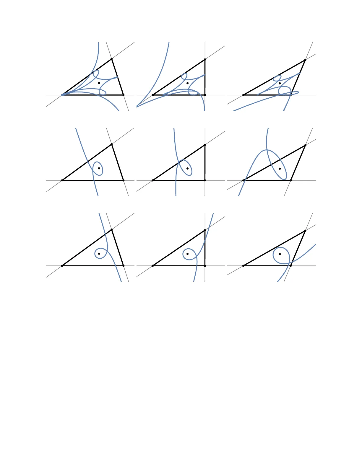
(SEMI-)INV ARIANT CUR VES FR OM CENTERS OF TRIANGLE F AMILIES KLARA MUNDILO V A AND OLIVER GROSS Abstract. W e study curv es obtained by tracing triangle centers within special families of triangles, fo cusing on cen ters and families that yield (semi-)inv arian t triangle curves, meaning that v arying the initial triangle c hanges the loci only by an aﬃne transformation. W e iden tify four tw o-parameter families of triangle centers that are semi-inv ariant and determine which are in v ariant, in the sense that the resulting curv es for diﬀeren t initial triangles are related b y a similarity transformation. W e further observe that these centers, when com bined with the aliquot triangle family , yield sheared Maclaurin trisectrices, whereas the nedian triangle family yields Lima¸ con trisectrices. Keyw ords: triangle cen ters; loci of triangle centers; aﬃne inv ariance; similarit y in v ariance; Maclau- rin trisectrix; Lima¸ con trisectrix; plane algebraic curv es MSC 2020: 51M15, 51M04, 14H50, 51N10, 51N20 “T o me, this was weir d.” D. Hofstadter 1 1. Introduction Giv en a triangle, a num b er of quantities and ob jects can b e asso ciated with it, arguably the simplest b eing its side lengths and interior angles. In addition, there are selected p oin ts suc h as the centroid, the circumcenter, and the F ermat p oint, whic h are well-kno wn represen tatives of so- called triangle c enters . The study of triangle cen ters can b e traced back to the ancient Greeks and, pioneered b y Kimberling [ 7 , 6 ], it also enjoys attention in contemporary researc h [ 1 , 11 ]. Notably , the study of selected conﬁgurations of triangle centers led to the disco very of sp ecial algebraic curv es asso ciated to triangles [ 2 , 3 ]. F or example, the Balaton curv e—whic h contains a triangles ortho cen ter, circumcen ter, in-cen ter, T oricelli’s point, and ﬁrst isodynamic p oint—is algebraic for certain triangles [ 4 ]. Other lines of work examine curv es asso ciated to triangles obtained by tracing p oin ts (or tri- angle cen ters) in a one-parameter family of triangles. Examples of such families include poristic triangles [ 12 ] and triangles obtained by linearly displacing one of the triangle’s v ertices [ 5 , 9 ]. Aliquot and nedian triangles are notable examples of triangle families in which the cen troids are concurren t [ 13 ]. Ko drnja and Koncul [ 8 ] describ e the lo ci of the vertices of nedian triangles, while Mundilo v a [ 10 ] demonstrates that the ﬁrst isogonic and isodynamic cen ters of aliquot triangles trace an algebraic curve, the Maclaurin trise ctrix , regardless of the initial triangle. Inspired by the functional deﬁnition of triangle cen ters, we introduce the concept of Ψ -triangle families, whic h includes the aliquot and nedian families as prominent examples. The cen tral theme of this w ork is the study of curv es traced by triangle centers as the underlying triangle v aries within suc h a family . W e identify triangle centers, and com binations thereof that give rise to curves with strong geometric rigidity . Under changes of the reference triangle, they transform merely by aﬃne or even similarity transformations. T o formalize this notion, we distinguish b et ween t wo t yp es of rigidit y . A triangle curv e is called semi-invariant if, under a change of the reference triangle, the curv e traced by a given triangle cen ter Date : F ebruary 26, 2026. 1 T aken from the forew ord in [ 7 ]. 1 2 KLARA MUNDILO V A AND OLIVER GR OSS c hanges only by an aﬃne transformation, namely translations, rotations, scaling, or sheering. A curv e is called invariant if it is semi-inv arian t without allowing sheering. 1.1. Outline. This paper is organized as follows. In Section 2 , w e review the deﬁnition of triangle cen ters and summarize a selection of prop erties that will b e used throughout the pap er. In Section 3 , w e introduce Ψ -triangle families and show that they form a geometric structure of indep endent in terest. In particular, we prov e that the set of triangle families, equipp ed with concatenation, carries the structure of an Ab elian group. Our main results are presented in Section 4 . W e ﬁrst study local and global properties of triangle curv es in Section 4.1 , with emphasis on semi-inv ariance and in v ariance. W e sho w that the prop erty of a triangle center generating a semi-in v arian t curve with resp ect to the aliquot family extends to a broad class of Ψ -triangle families. W e also pro v e that in v ariance is preserved under concatenation of families. Building on work of Mundilo v a [ 10 ], who show ed that t wo triangle centers generate Maclaurin trisectrices when combined with the aliquot family , w e substantially extend this result in Section 4.2 . W e iden tify four tw o-parameter families of semi-in v ariant triangle cen ters with resp ect to the class of decomposable triangle families. Within these families, we characterize those triangle centers that giv e rise to in v ariant curv es. W e sho w that in the sp ecial case of aliquot or nedian triangle families, the resulting curves are sheared Maclaurin or Lima¸ con trisectrices, resp ectively . Finally , in Section 4.3 , w e address an in verse problem. F or the semi-inv ariant curv e-generating triangle centers identiﬁed in Section 4.2 , w e determine the Ψ -triangle family that pro duces a pre- scrib ed admissible target curve. Before turning to the study of triangle cen ters, w e ﬁx notation and con ven tions that will be used throughout the pap er. F or readability , we present the main concepts and results in the b o dy of the pap er. Unless stated otherwise, pro ofs are deferred to the app endix. 1.2. Notation. An y distinct three p oints A , B , C ∈ R 2 uniquely deﬁne a triangle ∆ with edges a , b , and c opposite the resp ective vertices, whose lengths w e denote b y a, b, c ≥ 0 resp ectively . Additionally , we follow the conv ention to lab el the angles incident to the vertices A , B , and C by α , β , and γ , resp ectively (see Figure 1 ). In the following, w e consider only triangles ∆ that are non-degenerate, i.e. , the three v ertices are assumed to b e in general p osition. W e denote the set of all such triangles by △ : = { ∆ | A , B , C ∈ R 2 are distinct and non-collinear p oints } . W e can equiv alently describ e the set of non-degenerate triangles in terms of their side-lengths, i.e. , triples ( a, b, c ) ∈ R 3 > 0 suc h that a < b + c , b < c + a and c < a + b . F or brevity , and b y sligh t abuse of notation w e will denote the set of suc h triples also by △ . Using Her on ’s formula , we express the area of the triangle as area(∆) = 1 4 p ( a + b + c )( − a + b + c )( a − b + c )( a + b − c ) . Note that area(∆)  = 0 for ∆ ∈ △ . T o keep the in parts lengthy equations as concise as p ossible w e emplo y tw o sets of co ordinate systems throughout the pap er, whic h b oth sp ecify p oin ts in the plane in terms of the vertex p ositions A , B , C ∈ R 2 . First, w e consider homo gene ous b aryc entric c o or dinates [ λ 1 : λ 2 : λ 3 ] T , denoted as column vectors, which determine the p osition of a p oint P ∈ R 2 b y P = 1 λ 1 + λ 2 + λ 3 ( λ 1 A + λ 2 B + λ 3 C ) . (SEMI-)INV ARIANT CUR VES FROM CENTERS OF TRIANGLE F AMILIES 3 A B C c a b α β γ A B C [ x 1 : x 2 : x 3 ] x 1 x 2 x 3 A B C   λ 1 λ 2 λ 3   λ 3 λ 1 λ 2 Figure 1. Illustration of the notation used in this pap er, highligh ting geometric in terpretations of barycentric co ordinates (cen ter) and trilinear co ordinates (righ t). They can b e normalize d b y asking that λ 1 + λ 2 + λ 3 = 1. In contrast, homo gene ous triline ar c o or dinates [ x 1 : x 2 : x 3 ], denoted as ro w v ectors, determine the same p oin t P as P = 1 aλ 1 + bλ 2 + cλ 3 ( ax 1 A + bx 2 B + cx 3 C ) . Whenev er it is reasonably deﬁned, the conv ersion b etw een co ordinates of these tw o sets of co ordi- nate systems is ac hieved b y division or m ultiplication with the triangle’s side lengths: [ x 1 : x 2 : x 3 ] =   λ 1 / a λ 2 / b λ 3 / c   , r esp.   λ 1 λ 2 λ 3   = [ ax 1 : bx 2 : cx 3 ] . Consequen tly , division of the expressions ax 1 , bx 2 , cx 3 b y ax 1 + bx 2 + cx 3 yields the conv ersion from trilinear to normalized barycen tric co ordinates. 2. Triangle Centers 2.1. Deﬁnition and preliminaries. The following deﬁnition of a triangle center is adapted from Kim b erling [ 7 ]. Deﬁnition 1. A function ψ : △ → R , ψ ≡ 0 , is said to b e a triangle center function if it is (i) homogeneous , i.e. , ther e exists some c onstant r ∈ R such that for al l t > 0 we have ψ ( ta, tb, tc ) = t r ψ ( a, b, c ) . (1) In this p ap er, we wil l use the notation deg ( ψ ) = r to indic ate that ψ has homo geneity r . (ii) bi-symmetric in the se c ond and thir d variables, i.e. , for al l a, b, c ∈ △ , we have ψ ( a, b, c ) = ψ ( a, c, b ) . (2) The set of al l triangle c enter functions is denote d by T . Each ψ ∈ T deﬁnes a triangle center of ( a, b, c ) ∈ △ with triline ar c o or dinates X ψ = [ ψ ( a, b, c ) : ψ ( b, c, a ) : ψ ( c, a, b )] . While Kim b erling only considers p ositive r , our deﬁnition also allows for negative r , as the degree of homogeneity of an y triangle center function can b e increased, for example, by m ultiplying b y pow ers of abc . Additionally , note that the deﬁnition of a triangle cen ter is equiv arian t under similarit y transformations, i.e. , under translations, rotations, reﬂections, and uniform scalings. That is, the center of the transformed triangle is the same point as the transformed cen ter of the original triangle. T o describ e triangle cen ter functions that corresp ond to the same triangle centers, w e introduce: 4 KLARA MUNDILO V A AND OLIVER GR OSS X i Name ϕ i ( a, b, c ) traceable X − 1 i X 1 Incen ter 1 y es X 1 X 2 Cen troid a − 1 y es X 6 X 3 Circumcen ter a ( − a 2 + b 2 + c 2 ) y es X 4 X 6 Symmedian p oint a y es X 2 X 11 F euerbac h p oin t bc ( − a + b + c )( b − c ) 2 no X 59 X 13 First isogonic center csc ( α − π / 3 ) y es X 15 X 14 Second isogonic center csc ( α + π / 3 ) y es X 16 X 15 First iso dynamic center sin ( α − π / 3 ) y es X 13 X 16 Second iso dynamic center sin ( α + π / 3 ) y es X 14 T able 1. Selection of centers and their generating functions. Deﬁnition 2. We denote by Cyc( T ) the subset of functions in T that ar e nowher e vanishing, i.e. , f ( a, b, c )  = 0 for al l ( a, b, c ) ∈ △ and inv ariant under cyclic p ermutations , that is, f ( a, b, c ) ∈ Cyc( T ) satisﬁes f ( a, b, c ) = f ( b, c, a ) = f ( c, a, b ) . The following Lemma 1 , which is an immediate consequence of Deﬁnition 2 , clariﬁes when tw o triangle cen ter functions represen t the same triangle cen ter, namely when they diﬀer by a cyclic factor. Lemma 1. Two triangle c enter functions ψ 0 ( a, b, c ) and ψ 1 ( a, b, c ) describ e the same triangle c enter if ψ 1 ( a, b, c ) = f ( a, b, c ) ψ 0 ( a, b, c ) , for some f ( a, b, c ) ∈ Cyc( T ) . We wil l indic ate that two triangle c enter functions ψ 0 and ψ 1 describ e the same triangle c enter by ψ 0 ∼ = ψ 1 . Remark 1. Sinc e abc ∈ Cyc( T ) , we have ψ ∼ = abc ψ for al l ψ ∈ T . Thus, in Deﬁnition 1 , homo geneity is the essential r e quir ement, wher e as the p articular de gr e e c an b e shifte d by multiplying by p owers of abc and ther efor e has no ge ometric signiﬁc anc e (on nonde gener ate triangles). T riangle centers are tied together by sev eral natural dualities, and among the most useful is the passage to an isogonal conjugate. In this setting, isogonal conjugation acts on the data deﬁning a cen ter by inv erting the asso ciated triangle center function, producing a new center that is paired with the original one. Deﬁnition 3. Given a triangle c enter X ψ , its isogonal conjugate X ψ − 1 is a triangle c enter that c orr esp onds to the triangle c enter function ψ − 1 ( a, b, c ) : = ( ψ ( a, b, c )) − 1 . The set of triangle cen ter functions T is kno wn to be a con tinuum. A catalog of more than 60,000 distinct, num b ered triangle centers is a v ailable in the Encyclop e dia of T riangle Centers [ 6 ]. A selection of cen ters addressed in the presen t work along with their isogonal conjugates, is presen ted in T able 1 . Con v ention. In this paper, we use ψ j to denote a generic triangle center function and ϕ i to refer to the triangle cen ter function corresponding to a sp eciﬁc, n umbered triangle center (according to [ 6 ]). That is, ϕ i represen ts the triangle cen ter function for the i -th triangle center X i . F or the isogonal conjugate of a triangle center X ψ i w e also abbreviate X − 1 ψ i : = X ψ − 1 i . 2.2. Prop erties of triangle centers. While the deﬁnition of triangle centers is broad and cap- tures many desirable features, it do es not impose strong constrain ts on triangle cen ter functions. F or instance, not all such functions yield triangle centers that hav e a w ell-deﬁned representativ e in the Euclidean plane for all triangles, and some centers may coincide with others for multiple triangle conﬁgurations. In this section, we introduce terminology to rule out these pathologies. (SEMI-)INV ARIANT CUR VES FROM CENTERS OF TRIANGLE F AMILIES 5 2.2.1. T r ac e able triangle c enters. While triangle cen ter functions typically describ e homogeneous co ordinates, it is sometimes adv antageous to work with triangle center functions in a normalized form. Deﬁnition 4. Given a triangle c enter function ψ ∈ T , its trace is given by Σ ψ ( a, b, c ) = a ψ ( a, b, c ) + b ψ ( b, c, a ) + c ψ ( c, a, b ) . We say that the triangle c enter function ψ ∈ T is traceable if its tr ac e is nowher e vanishing, i.e. , Σ ψ ( a, b, c )  = 0 for al l ( a, b, c ) ∈ △ , and normalized if Σ ψ ( a, b, c ) ≡ 1 . Mor e over, a triangle c enter is said to b e tr ac e able whenever its deﬁning triangle c enter function is. It follo ws from the deﬁnition of triangle cen ters that traceable triangle cen ters are those that corresp ond to well-deﬁned p oints in R 2 for all ∆ ∈ △ . Examples of suc h cen ters are listed 2 in T able 1 . Notably , the F euerbac h p oin t X 11 is not traceable, since Σ ϕ 11 ( a, a, a ) = 0. Finally , w e note that the well-deﬁnedness of Deﬁnition 4 follows from the prop erties outlined in the follo wing prop osition, which are direct consequences of the prop erties of triangle center functions. Prop osition 1. L et ψ ∈ T b e a triangle c enter function of de gr e e k ≥ 0 and f ∈ Cyc( T ) . Then, (i) Σ ψ ( a, b, c ) = Σ ψ ( b, c, a ) = Σ ψ ( c, a, b ) , (ii) Σ ψ ( a, b, c ) = Σ ψ ( a, c, b ) , (iii) Σ ψ ( ta, tb, tc ) = t k +1 Σ ψ ( a, b, c ) , (iv) Σ f ψ ( a, b, c ) = f ( a, b, c ) Σ ψ ( a, b, c ) . That is, Σ ψ ∈ T is wel l deﬁne d on the e quivalenc e classes of triangle c enter functions which describ e the same triangle c enters and homo gene ous of deg (Σ ψ ) = k + 1 . Note that, if ψ is traceable, Σ ψ ∈ Cyc( T ). That is, any traceable triangle cen ter function ψ ∈ T can b e normalized by ψ 7→ 1 Σ ψ ψ . With the ab ov e prop erties, the following Prop osition is easy to verify . Prop osition 2. Normalize d triangle c enter functions have homo geneity de gr e e -1. 2.2.2. Essential ly diﬀer ent triangle c enters. F or an equilateral triangle with side lengths a > 0, the trace of an y triangle center function ψ ∈ T simpliﬁes to Σ ψ ( a, a, a ) = 3 aψ ( a, a, a ). If ψ ( a, a, a )  = 0, whic h is the case for traceable triangle cen ters, the triangle center has barycentric co ordinates X ψ =   a ψ ( a, a, a ) a ψ ( a, a, a ) a ψ ( a, a, a )   ∼ =   1 1 1   = X 2 . So, all traceable triangle cen ters coincide with the centroid of the triangle in equilateral triangles. Since this coincidence constitutes a degenerate scenario, w e will mainly fo cus our attention on triangle centers that do not coincide, or are diﬀer ent , for all other triangles. Deﬁnition 5. We c al l two triangle c enter functions ψ 0 , ψ 1 ∈ T essentially diﬀerent , if the c orr e- sp onding triangle c enters c oincide only in e quilater al triangles. F or example, in a right-angled isosceles triangle, the triangle centers X 3 and X 63 coincide at the midp oint of the h yp otenuse. Consequently , the triangle cen ters are therefore not essen tially diﬀeren t (see Section A , Example 4 ). The follo wing lemma provides pairs of essen tially diﬀeren t triangle centers that are considered in later sections of this pap er. 2 The computations used to determine traceabilit y and non-traceability are provided in Appendix A , Example 2 and Example 3 . 6 KLARA MUNDILO V A AND OLIVER GR OSS T ψ 0 ψ 1 span Cyc( T ) ( ψ 0 , ψ 1 ) A B C X ψ 0 X ψ 1 span Cyc( T ) ( X ψ 0 , X ψ 1 ) Figure 2. Illustration of the space of triangle functions. Lemma 2. (i) The triangle c enters X 3 and X 6 ar e essential ly diﬀer ent. (ii) The triangle c enters X 13 , X 14 , X 15 , and X 16 ar e essential ly diﬀer ent fr om the c entr oid X 2 . 2.3. Collinear triangle centers. The study of triangle cen ters also examines their relationships, suc h as collinearity . Recall that three triangle centers X ψ 0 , X ψ 1 , X ψ 2 are collinear, if for all ( a, b, c ) ∈ △ det  X ψ 0 X ψ 1 X ψ 2 1 1 1  = 0 . (3) Consequen tly , for triangles ∆ ∈ △ for which Σ ψ 0 , Σ ψ 1 , Σ ψ 2  = 0, we deﬁne M ∆ =  A B C 1 1 1  and M ψ =   a ψ 0 ( a,b,c ) / Σ ψ 0 a ψ 1 ( a,b,c ) / Σ ψ 1 a ψ 2 ( a,b,c ) / Σ ψ 2 b ψ 0 ( b,c,a ) / Σ ψ 0 b ψ 1 ( b,c,a ) / Σ ψ 1 b ψ 2 ( b,c,a ) / Σ ψ 2 c ψ 0 ( c,a,b ) / Σ ψ 0 c ψ 1 ( c,a,b ) / Σ ψ 1 c ψ 2 ( c,a,b ) / Σ ψ 2   , and rewrite det  X ψ 0 X ψ 1 X ψ 2 1 1 1  = det ( M ∆ · M ψ ) = det ( M ∆ ) det ( M ψ ) . Since the vertices of a triangle ∆ ∈ △ are in general p osition, det( M △ )  = 0, Equation ( 3 ) is equiv alen t to det( M ψ ) = 0. Then, due to the m ultilinearit y of the determinant, w e m a y simplify det( M ψ ) = abc Σ ψ 0 Σ ψ 1 Σ ψ 2 det   ψ 0 ( a, b, c ) ψ 1 ( a, b, c ) ψ 2 ( a, b, c ) ψ 0 ( b, c, a ) ψ 1 ( b, c, a ) ψ 2 ( b, c, a ) ψ 0 ( c, a, b ) ψ 1 ( c, a, b ) ψ 2 ( c, a, b )   . As w e fo cus on non-degenerate triangles, a necessary and suﬃcient condition for the collinearit y of three triangle cen ters is the linear dep endence of triples corresp onding to triangle center functions ev aluated at cyclic p ermutation triangle edge lengths. 2.3.1. Cyclic-aﬃne triangle c enter c ombinations. W e now formalize a simple but ﬂexible notion of linear dep endence among triangle cen ter functions, where the co eﬃcients are allow ed to v ary cyclically with ( a, b, c ). Deﬁnition 6. L et ψ 0 , ψ 1 ∈ T b e two triangle c enter functions and ω 0 , ω 1 ∈ Cyc( T ) such that deg( ω 0 ψ 0 ) = deg( ω 1 ψ 1 ) . We r efer to the triangle c enter function ψ ω ( a, b, c ) = ω 0 ( a, b, c ) ψ 0 ( a, b, c ) + ω 1 ( a, b, c ) ψ 1 ( a, b, c ) , (4) as a cyclic-aﬃne combination of ψ 0 and ψ 1 . We denote the set of cyclic-aﬃne c ombinations of ψ 0 and ψ 1 by span Cyc( T ) ( ψ 0 , ψ 1 ) . (SEMI-)INV ARIANT CUR VES FROM CENTERS OF TRIANGLE F AMILIES 7 It is straigh tforw ard to v erify that ψ ω in Equation ( 4 ) is a triangle center function, and therefore is well deﬁned. Remark 2. Note that even if the two triangle c enter functions in L emma 6 ar e tr ac e able, the c orr esp onding cyclic-aﬃne c ombination ne e d not b e. In p articular, for normalize d triangle c enter functions ψ 0 and ψ 1 , ω 0 ∈ Cyc( T ) , and ω 1 = − ω 0 , we have Σ ψ ω ( a, b, c ) = 0 for al l ∆ ∈ △ . The next lemma shows that cyclic-aﬃne combinations behav e lik e gen uine aﬃne com binations at the level of p oints: whenev er the combination is traceable, the resulting cen ter lies on the line through X ψ 0 and X ψ 1 , with weigh ts determined by the cyclic co eﬃcients, see Figure 2 . Lemma 3. L et ψ ω ∈ span Cyc( T ) ( ψ 0 , ψ 1 ) b e tr ac e able. Then, the asso ciate d triangle c enters ar e c ol line ar and given by X ψ ω = ω 0 Σ ψ 0 ω 0 Σ ψ 0 + ω 1 Σ ψ 1 X ψ 0 + ω 1 Σ ψ 1 ω 0 Σ ψ 0 + ω 1 Σ ψ 1 X ψ 1 . (5) In addition, we have that ψ ω ∈ span Cyc( T ) ( ψ 0 , ψ 1 ) = ⇒ ψ 1 ∈ span Cyc( T ) ( ψ 0 , ψ ω ) . Note, how ever, that somewhat counterin tuitively ψ 0 , ψ 1 ∈ span Cyc( T ) ( ψ 0 , ψ 1 ) since, by Deﬁni- tion 2 , ω 0 , ω 1 ≡ 0. Consequen tly , span Cyc( T ) ( ψ 0 , ψ 1 )  = span Cyc( T ) ( ψ 0 , ψ ω ). A k ey p oin t is that this construction depends only on the underlying triangle cen ters, not on how w e choose to represen t them. In particular, rescaling ψ 0 and ψ 1 b y cyclic factors do es not c hange the family of cyclic-aﬃne combinations they generate. Lemma 4. The set of cyclic-aﬃne c ombinations of two triangle c enters functions ψ 0 and ψ 1 is indep endent of the choic e of their r epr esentatives. That is, span Cyc( T ) ( f 0 ψ 0 , f 1 ψ 1 ) = span Cyc( T ) ( ψ 0 , ψ 1 ) , wher e f 0 , f 1 ∈ Cyc( T ) . Conse quently, we may also r efer to the set of triangle c enters X ψ ω c orr e- sp onding to cyclic-aﬃne triangle c enter functions of ψ 0 and ψ 1 as span Cyc( T ) ( X ψ 0 , X ψ 1 ) . It is known that the line connecting X 3 and X 6 , the so-called Br o c ar d axis , contains the ﬁrst iso dynamic center X 15 . Example 5 in App endix A illustrates X 15 as a cyclic-aﬃne combination of X 3 and X 6 . Finally , w e discuss under whic h conditions span Cyc( T ) ( X ψ 0 , X ψ 1 ) contains all triangle cen ters that are essentially diﬀeren t from X ψ 0 and X ψ 1 . Lemma 5. If two distinct triangle c enters X ψ 0 and X ψ 1 ar e b oth tr ac e able, then span Cyc( T ) ( X ψ 0 , X ψ 1 ) c ontains al l tr ac e able triangle c enters that ar e c ol line ar with X ψ 0 and X ψ 1 and ar e essential ly dif- fer ent fr om these two c enters. 2.3.2. Constant-aﬃne triangle c enter c ombinations. Next, we highlight a subset of collinear triangle cen ters whose co eﬃcien ts do not dep end on the shape of the triangle, i.e. , are constan t with resp ect to the triangle edge lengths a , b , and c . Deﬁnition 7. L et ψ 0 and ψ 1 b e two triangle c enter functions with deg ( ψ 0 ) = deg( ψ 1 ) and γ 0 , γ 1 ∈ R \ { 0 } . We r efer to the triangle c enter function ψ λ 0 : λ 1 ( a, b, c ) = λ 0 ψ 0 ( a, b, c ) + λ 1 ψ 1 ( a, b, c ) , as a constant-aﬃne com bination of ψ 0 and ψ 1 . We denote the set of c onstant-aﬃne c ombinations of ψ 0 and ψ 1 by span const ( ψ 0 , ψ 1 ) . Since constan t-aﬃne combinations of triangle cen ters are a sp ecial case of cyclic-aﬃne com bina- tions, a sp ecial case of Lemma 3 applies verbatim in this setting. 8 KLARA MUNDILO V A AND OLIVER GR OSS Prop osition 3. L et ψ λ 0 : λ 1 ∈ span const ( ψ 0 , ψ 1 ) b e tr ac e able. Then, the asso ciate d triangle c enters ar e c ol line ar and given by X ψ λ 0 : λ 1 = λ 0 Σ ψ 0 λ 0 Σ ψ 0 + λ 1 Σ ψ 1 X ψ 0 + λ 1 Σ ψ 1 λ 0 Σ ψ 0 + λ 1 Σ ψ 1 X ψ 1 . (6) In addition, we have that ψ λ 0 : λ 1 ∈ span const ( ψ 0 , ψ 1 ) = ⇒ ψ 1 ∈ span const ( ψ 0 , ψ λ 0 : λ 1 ) . Note that if the t wo triangle cen ter functions ψ 0 and ψ 1 in Lemma 3 are normalized and therefore ha v e homogeneity degree − 1, b oth the co eﬃcients of the triangle center function and the triangle cen ters are constan t and the resulting triangle center function ψ λ 0 : λ 1 is normalized. If, in addition, λ 0 + λ 1 = 1, the co eﬃcients of the triangle cen ter function and the triangle center are the same. Notably , constant-aﬃne combinations pro duce families of triangle cen ters that are pairwise es- sen tially diﬀerent. Lemma 6. If the triangle c enter functions ψ 0 and ψ 1 in L emma 3 c orr esp ond to essential ly diﬀer ent tr ac e able triangle c enters, then for λ 0 , λ 1  = 0 , the triangle c enters c orr esp onding to ψ λ 0 : λ 1 ar e essential ly diﬀer ent fr om ψ 0 and ψ 1 . A dditional ly, if λ 0 / λ 1  = λ 0 / λ 1 , then the triangle c enter functions ψ λ 0 : λ 1 and ψ λ 0 : λ 1 ar e essential ly diﬀer ent. Finally , note that, unlik e cyclic-aﬃne com binations, constant-aﬃne combinations dep end on the c hoice of triangle cen ter functions. Nevertheless, using three collinear triangle centers, we can deﬁne a set of constant-aﬃne combinations that are indep endent of the speciﬁc choice of triangle cen ter function. F or more information, see App endix A , Lemma 13 . An example of families of constan t-aﬃne triangle centers within the Bro card axis is provided in Example 6 . 3. Ψ -Triangle f amilies In this section, we explore families of triangles that can b e deriv ed from a giv en triangle ∆ ∈ △ . Inspired by Kimberling’s approac h, which emplo ys triangle center functions as abstract to ols for studying triangle centers, w e describ e these triangle families in terms of triplets of functions. Deﬁnition 8. A Ψ -triangle family t 7→ ∆ Ψ t ∈ △ is determine d by a triangle ∆ ∈ △ and thr e e sc alar value d functions Ψ i ( t ) , Ψ : R → R 3 , t 7→   Ψ 1 ( t ) Ψ 2 ( t ) Ψ 3 ( t )   , such that Ψ 1 ( t ) + Ψ 2 ( t ) + Ψ 3 ( t )  = 0 and not Ψ 1 ( t ) ≡ Ψ 2 ( t ) ≡ Ψ 3 ( t ) . In terms of the b aryc entric c o or dinates with r esp e ct the vertic es A , B , and C of ∆ , the vertic es of ∆ Φ t ar e given by A Ψ t =   Ψ 1 ( t ) Ψ 2 ( t ) Ψ 3 ( t )   , B Ψ t =   Ψ 3 ( t ) Ψ 1 ( t ) Ψ 2 ( t )   , C Ψ t =   Ψ 2 ( t ) Ψ 3 ( t ) Ψ 1 ( t )   . In the fol lowing, we r efer to the thr e e functions Ψ 1 ( t ) , Ψ 2 ( t ) , and Ψ 3 ( t ) as the generating functions of the family ∆ Ψ t . A dditional ly, we c al l a triangle family interpolating , if ∆ Ψ t = ∆ for some t . Similar to triangle center functions, we follo w the conv ention that generic triangle families are denoted by Ψ , and sp eciﬁc ones are represented by Φ with a subscript. F or example, Φ Id : t 7→   1 0 0   (7) (SEMI-)INV ARIANT CUR VES FROM CENTERS OF TRIANGLE F AMILIES 9 is the identit y mapping, and Φ S : t 7→   1 + 2 t 1 − t 1 − t   (8) represen ts a homothety with the centroid as the origin. The follo wing lemma identiﬁes tw o inv ariants of Ψ -triangle families that can serve as necessary conditions for a triangle family to b e classiﬁed as a Ψ -triangle family: Lemma 7. F or al l t ∈ R , the fol lowing statements hold: (i) The c entr oid of a triangle ∆ Ψ t c oincides with the c entr oid of ∆ . (ii) If ∆ is e quilater al, ∆ Ψ t is also e quilater al. This lemma provides a useful criterion for determining when a giv en triangle family is not a Ψ -triangle family . F or example, families of triangles obtained b y linear displacemen ts of one of the vertices, cannot b e examples of Ψ -triangle families as they do not preserve the cen troid [ 5 , 9 ]. Moreo v er, the centroids of P oristic triangles generically trace a circle [ 12 , Thm. 4.6]. 3.1. Concatenation of Ψ-triangle families. Having established some basic prop erties of Ψ - triangle families, it is natural to consider the concatenation of triples of generating functions cor- resp onding to tw o triangle families: Deﬁnition & Lemma 9. The c onc atenation of two triangle families, Ψ =   Ψ 1 Ψ 2 Ψ 3   , ˜ Ψ =   ˜ Ψ 1 ˜ Ψ 2 ˜ Ψ 3   , is a Ψ -triangle family given by Ψ ◦ ˜ Ψ : t 7→   Ψ 1 ˜ Ψ 1 + Ψ 2 ˜ Ψ 3 + Ψ 3 ˜ Ψ 2 Ψ 1 ˜ Ψ 2 + Ψ 2 ˜ Ψ 1 + Ψ 3 ˜ Ψ 3 Ψ 1 ˜ Ψ 3 + Ψ 2 ˜ Ψ 2 + Ψ 3 ˜ Ψ 1   . (9) Giv en that the set of all Ψ -triangle families is closed under concatenation, the following lemma lists additional algebraic prop erties of this structure: Lemma 8. The fol lowing pr op erties hold for al l Ψ -triangle families: (i) The c onc atenation of triangle families c ommutes: Ψ ◦ ˜ Ψ = ˜ Ψ ◦ Ψ . (ii) The c onc atenation of triangle families is asso ciative: Ψ ◦  ˜ Ψ ◦ ˆ Ψ  =  Ψ ◦ ˜ Ψ  ◦ ˆ Ψ . (iii) Φ Id is a neutr al element with r esp e ct to the c onc atenation, Ψ ◦ Φ Id = Ψ . (iv) Every Ψ -triangle family has an inverse, Ψ − 1 : t 7→   (Ψ 1 ) 2 − Ψ 2 Ψ 3 (Ψ 3 ) 2 − Ψ 1 Ψ 2 (Ψ 2 ) 2 − Ψ 3 Ψ 1   . Conse quently, the set of al l Ψ -triangle families in c ombination with the c onc atenation is an Ab elian gr oup with neutr al element Φ Id . 10 KLARA MUNDILO V A AND OLIVER GR OSS A B C C t A t B t ∆ Φ A t A B C C ′ t A ′ t B ′ t A t B t C t ∆ Φ N t Figure 3. Illustration of aliquot (left) and nedian (right) triangle families. 3.2. Aliquot and nedian triangle families. In this paper, t w o triangle families, the aliquot and the ne dian families asso ciated with a triangle [ 13 ], play an imp ortan t role. The former triangle family is obtained by equipping the triangle ∆ ∈ △ with vertices A , B and C with an orientation and deﬁning a new triple of v ertices A t , B t , C t suc h that the placement of the new vertices on the edges divides the resp ective edge in equal prop ortions (Figure 3 ). This can b e achiev ed by taking linear combinations A t = (1 − t ) B + t C , B t = (1 − t ) C + t A , C t = (1 − t ) A + t B . This construction can b e stated in terms of a Ψ -triangle family as follows: Deﬁnition 10. The aliquot family Φ A is deﬁne d by Φ A : t 7→   0 1 − t t   . (10) Instead of choosing p oints A ′ t , B ′ t , and C ′ t that determine the aliquot family as a new triangle, w e can choose A t , B t , and C t to b e resp ectiv e pairwise intersections of the lines ℓ AA ′ t , ℓ BB ′ t , and ℓ CC ′ t , see Figure 3 . This determines yet another Ψ -triangle family , the ne dian family Φ N , which can b e derived from an initial triangle as stated in the next lemma. Deﬁnition & Lemma 11. The nedian family Φ N is deﬁne d by Φ N : t 7→   (1 − t ) t t 2 (1 − t ) 2   . (11) The following prop osition collects basic geometric prop erties of the aliquot and nedian families, all of which follo w directly from the deﬁnitions and are illustrated in Figure 4 . Prop osition 4. L et ∆ = ( A , B , C ) b e a triangle in △ , X 2 its c entr oid. (i) The aliquot and ne dian families of a triangle ar e interp olating. Sp e ciﬁc al ly, ∆ Φ A 0 = ( B , C , A ) , ∆ Φ A 1 = ( C , A , B ) , ∆ Φ N 0 = ( C , A , B ) , and ∆ Φ N 1 = ( A , B , C ) . (ii) ∆ Φ A 1 / 2 is r elate d to the original triangle by a sc aling of 1 / 2 with r esp e ct to X 2 fol lowe d by a p oint inversion thr ough X 2 . (iii) The triangles ∆ Φ A 1 / 3 and ∆ Φ A 2 / 3 r elate by a p oint inversion thr ough X 2 . (iv) The triangle ∆ Φ N 1 / 2 de gener ates to X 2 . (SEMI-)INV ARIANT CUR VES FROM CENTERS OF TRIANGLE F AMILIES 11 A B C ∆ Φ A 1 / 3 ∆ Φ A 1 / 2 ∆ Φ A 2 / 3 X 2 A B C ∆ Φ N 1 / 3 ∆ Φ N 2 / 3 ∆ Φ N 1 / 2 Figure 4. Illustrations of prop erties of aliquot and nedian triangle families dis- cussed in Lemma 4 . In addition to these results, we sho w a connection betw een the Ψ -triangle families in tro duced so far and their inv erses. Although these observ ations hav e no direct implications for the theory dev elop ed in the next section, we ﬁnd them nonetheless noteworth y . Lemma 9. The Ψ -triangle families Φ S , Φ A , and Φ N r elate to their inverses as fol lows: • F or t  = 0 , the inverse of the family of sc ale d triangles in Equation ( 8 ) is a sc aling by 1 t , Φ − 1 S ( t ) = Φ S  1 t  . • F or t  = 1 / 2 , the inverse of the aliquot family in Equation ( 10 ) is a memb er of the ne dian family, Φ − 1 A ( t ) = Φ N  − t 1 − 2 t  . • F or t  = 1 / 2 , the inverse of the ne dian family in Equation ( 11 ) is a memb er of the aliquot family, Φ − 1 N ( t ) = Φ A  − t 1 − 2 t  . Finally , we note that b y concatenation of the of the aliquot and nedian families w e can obtain a w ealth of non-trivial examples of Ψ -families. 3.3. Relating triangle families to the aliquot family . Finally , we sho w which Ψ -triangle families relate to the aliquot family through appropriate scaling and reparametrization. This ob- serv ation will pla y an imp ortant role at sev eral p oints in the next section. Before w e con tinue, we ﬁrst introduce the follo wing subset of Ψ -triangle families: Deﬁnition 12. Given a Ψ -triangle family, deﬁne δ Ψ ( t ) = 2Ψ 1 ( t ) − Ψ 2 ( t ) − Ψ 3 ( t ) ∈ R . We r efer to a Ψ -triangle family as decomp osable , if for al l t ∈ R , the c ondition δ Ψ ( t ) = 0 implies Ψ 1 ( t ) = Ψ 2 ( t ) = Ψ 3 ( t ) . Geometrically , a decomp osable Ψ -triangle family do es not con tain a triangle ∆ Ψ t whose v ertices are p ositioned in the follo wing conﬁguration (see Figure 5 ). F or a triangle ∆ ∈ △ , let ℓ AB , ℓ BC , and ℓ CA denote the three lines that pass through the centroid X 2 and are parallel to AB , BC , and CA , resp ectively . The triangle family is called decomp osable if, for all t ∈ R , A Ψ t , B Ψ t , C Ψ t lying on the lines ℓ BC , ℓ CA , and ℓ AB , resp ectively , implies that A Ψ t = B Ψ t = C Ψ t = X 2 . 12 KLARA MUNDILO V A AND OLIVER GR OSS A B C X 2 C Ψ t B Ψ t A Ψ t ∆ Ψ t Figure 5. Illustration of a triangle in a not decomp osable triangle family Ψ . Straigh tforw ard computations v erify that non-trivial examples of decomp osable families include the aliquot family Φ A and the nedian family Φ N . On the other hand, an example of a not decom- p osable family is Ψ : t 7→   1 − t t 0   , since δ Ψ (2) = 0, but Ψ (2) = ( − 1 , 2 , 0). The next lemma justiﬁes the term de c omp osable by demonstrating that each triangle family in this class can b e expressed as a comp osition of simpler, well-understoo d transformations, making the underlying structure explicit. Lemma 10. A de c omp osable Ψ -triangle family al lows a de c omp osition Ψ ( t ) = Φ S ( σ ( t )) ◦ Φ A ( τ ( t )) . wher e σ ( t ) = − 2Ψ 1 ( t ) − Ψ 2 ( t ) − Ψ 3 ( t ) Ψ 1 ( t ) + Ψ 2 ( t ) + Ψ 3 ( t ) and τ ( t ) = Ψ 1 ( t ) − Ψ 3 ( t ) 2Ψ 1 ( t ) − Ψ 2 ( t ) − Ψ 3 ( t ) . (12) If Ψ 1 ( t ) = Ψ 2 ( t ) = Ψ 3 ( t ) , then σ ( t ) = 0 while τ ( t ) is undeﬁne d. Pr o of. T o arriv e at constraints for σ ( t ) and τ ( t ), we compare a normalized form of Ψ ( t ) and Φ S ( σ ( t )) ◦ Φ A ( τ ( t )). Sp eciﬁcally , b y using the normalized v ersion of the expression in Equation ( 9 ) (or directly Equation ( 29 )), we obtain Ψ 1 ( t ) Ψ 1 ( t ) + Ψ 2 ( t ) + Ψ 3 ( t ) = 1 3 (1 − σ ( t )) Ψ 2 ( t ) Ψ 1 ( t ) + Ψ 2 ( t ) + Ψ 3 ( t ) = 1 3 (1 + σ ( t ) (2 − 3 τ ( t ))) (13) Ψ 3 ( t ) Ψ 1 ( t ) + Ψ 2 ( t ) + Ψ 3 ( t ) = 1 3 (1 − σ ( t ) (1 − 3 τ ( t ))) . Solving the ﬁrst equation for σ ( t ) results in the stated expression for σ ( t ). Inserting σ ( t ) into the second and third equations simpliﬁes to the same expression, namely , (2Ψ 1 ( t ) − Ψ 2 ( t ) − Ψ 3 ( t )) τ ( t ) = Ψ 1 ( t ) − Ψ 3 ( t ) . Note that if Ψ 1 ( t ) = Ψ 2 ( t ) = Ψ 3 ( t ), then σ ( t ) = 0 and τ ( t ) is undeﬁned. Otherwise, since Ψ is decomp osable, w e ha ve that 2Ψ 1 ( t ) − Ψ 2 ( t ) − Ψ 3 ( t )  = 0 and obtain the stated expression for τ ( t ). □ (SEMI-)INV ARIANT CUR VES FROM CENTERS OF TRIANGLE F AMILIES 13 Corollary 1. F or al l t ∈ R , we have Φ N ( t ) = Φ S ( σ ( t )) ◦ Φ A ( τ ( t )) , wher e τ ( t ) = 1 − t 1 − 2 t and σ ( t ) = (1 − 2 t ) 2 1 − t + t 2 . (14) 4. Triangle cur ves With these preparations in place, w e no w turn our atten tion to curves that are the locus of a triangle center in Ψ -triangle family: Deﬁnition 13. We c onsider curves t 7→ X Ψ ψ ( t ) tr ac e d by triangle c enters X ψ in a Ψ ( t ) -triangle family. We r efer to these as triangle curves . Remark 3. While we implicitly assume, as with triangle c enter functions, that triangle families ar e c ontinuous and gener al ly pr o duc e c ontinuous curves, this is not a pr er e quisite. Remark 4. Sinc e Ψ -triangle families of e quilater al triangles c onsist of e quilater al triangles (se e L emma 7 ), and tr ac e able triangle c enters c oincide with the c entr oid (se e Se ction 2.2.2 ), we exclude e quilater al triangles fr om the fol lowing discussion. 4.1. Prop erties of triangle curv es. Given a triangle cen ter and a triangle family , w e distinguish b et ween lo cal and global prop erties of the resulting triangle curv e. Lo cal properties focus on sp eciﬁc conﬁgurations and selected parameter v alues, such as whic h triangle centers are in terp olated by the triangle curv e. On the other hand, global prop erties analyze the ov erall geometry of the triangle curv e. F or some triangle families, it is relatively straightforw ard to determine the resulting triangle curv es. F or example, the triangle family of scaled triangles Φ S in Equation ( 8 ), the curv es X Φ S ψ ( t ) parametrize lines connecting X ψ to X 2 . While some triangle curves exhibit visual similarities, they generally dep end on the shap e of the underlying triangle, see Figure 6a . 4.1.1. L o c al pr op erties. In the following section, we presen t local features of triangle curv es, i.e. , prop erties corresp onding to sp eciﬁc parameter v alues, beginning with a prop erty that follows di- rectly from their deﬁnition: Prop osition 5. If ∆ Ψ t = ∆ , then X Ψ ψ ( t ) = X ψ . Ho w ever, in general, lo cal prop erties depend on the triangle family or triangle cen ter. The follo wing lemma summarizes features of triangle curv es deriv ed from the corresp onding prop erties of the aliquot and nedian triangle families, as presented in Prop osition 4 . Prop osition 6. L et Φ A r epr esent the aliquot triangle family describ e d in Equation ( 10 ) , Φ N the ne dian triangle family in Equation ( 11 ) , and let ψ ∈ T b e a triangle c enter function. (i) X ψ = X Φ A ψ (0) = X Φ A ψ (1) = X Φ N ψ (0) = X Φ N ψ (1) . (ii) X Φ A ψ ( 1 / 2 ) is the midp oint of X 2 and X Φ A ψ (0) , inverte d thr ough X 2 . (iii) X Φ A ψ ( 1 / 3 ) and X Φ A ψ ( 2 / 3 ) r elate d by an inversion thr ough X 2 . (iv) X Φ N ψ ( 1 / 2 ) = X 2 . 4.1.2. Semi-invariant triangle curves. Next, we examine t w o features in the study of global prop- erties of triangle curv es, b eginning with the concept of semi-invarianc e , see Figure 6b . Deﬁnition 14. If, for al l triangles ∆ ∈ △ , the curves t 7→ X Ψ ψ ( t ) diﬀer only by an aﬃne tr ansfor- mation, we r efer to the r esulting triangle curves as semi-inv ariant , and the c orr esp onding triangle c enter X ψ as a semi-inv ariant curv e-generating cen ter with r esp e ct to Ψ . 14 KLARA MUNDILO V A AND OLIVER GR OSS (a) T race of a generic triangle center ( X 59 ). (b) T race of a semi-inv ariant curve-generating center ( X 3 ). (c) T race of an inv ariant triangle curve-generating center ( X 13 ). Figure 6. Illustration of triangle curves for diﬀerent triangles of Φ A triangle fam- ilies. The cen trally lo cated p oints represent the triangle’s centroids. Note that this is a non-trivial requiremen t. F or most triangle cen ters, the connection b etw een the center and the triangle is of higher order (depending on the triangle’s side lengths), and the lo cation of triangle centers is not generally preserv ed under aﬃne transformations. Although it migh t initially seem coun terin tuitive that examples of non-trivial curves exist, Section 4.2 presents four tw o-parameter families of triangle centers that are related to tw o classical algebraic curves through aﬃne transformations. The next prop osition highlights a consequence of Lemma 7 that the existence of a non-trivial semi-in v ariant curv e-generating center X ψ with resp ect to a triangle family Ψ implies the existence of a one-parameter family of semi-inv ariant curve-generating cen ters with resp ect to the same family . Equiv alently , this also implies the existence of a one-parameter family of triangle families Ψ σ ( t ) for which X ψ is a semi-inv ariant curv e-generating center. Prop osition 7. F or ψ ∈ T , let X ψ b e a semi-invariant curve-gener ating c enter with r esp e ct to the family Ψ ( t ) , and let ψ σ c orr esp ond to the fol lowing c onstant-aﬃne c ombination of X ψ and the (SEMI-)INV ARIANT CUR VES FROM CENTERS OF TRIANGLE F AMILIES 15 c entr oid X 2 , that is, ψ σ ( a, b, c ) = (1 − σ ) ψ ( a, b, c ) Σ ψ ( a, b, c ) + σ ϕ 2 ( a, b, c ) Σ ϕ 2 ( a, b, c ) . for σ ∈ R \{ 0 , 1 } . • If Σ ψ σ  = 0 , the triangle c enters c orr esp onding to ψ σ ar e semi-invariant curve-gener ating c enters, with X Ψ ψ σ ( t ) = (1 − σ ) X Ψ ψ ( t ) + σ X 2 . (15) • Equivalently, X ψ is a semi-invariant curve-gener ating triangle c enter function with r esp e ct to the triangle families Ψ σ = Φ S ( σ ) ◦ Ψ , wher e Φ S ( σ ) denotes the sc aling w.r.t. X 2 by the sc alar factor σ ∈ R \{ 0 , 1 } as describ e d in Equation ( 8 ) . The r esulting one-p ar ameter families of semi-invariant triangle curves r elate by X Ψ ψ σ ( t ) = X Ψ σ ψ ( t ) . A dditional ly, it fol lows fr om L emma 6 that if X ψ is essential ly diﬀer ent fr om X 2 , the triangle c enters X ψ σ ar e essential ly diﬀer ent fr om X ψ and X 2 , and for σ  = σ , X ψ σ is essential ly diﬀer ent fr om X ψ σ . Note the imp ortance of com bining tw o normalized triangle cen ter functions in order to ensure that the co eﬃcien ts of the linear combination in Equation ( 15 ) do not dep end on the shap e of the triangle (unlike in Equation ( 6 )). In the next subsection, we use Proposition 7 to extend families of semi-inv ariant triangle cen ters by an additional parameter. T o this end, we deﬁne: Deﬁnition 15. Given a family of triangle-c enter functions Ω , we deﬁne its scaled family as Ω σ = { ψ σ | ψ ∈ Ω , σ ∈ R } . (16) The ab ov e Prop osition 7 sho ws that semi-inv ariance of a cen ter with resp ect to a non trivial triangle family automatically extends to a one-parameter family of triangle families. In the decom- p osable case, this observ ation can b e strengthened further: Lemma 11. If X ψ is semi-invariant with r esp e ct to a triangle family Ψ , then it r emains semi- invariant with r esp e ct to Φ S ( σ ( t )) ◦ Ψ ( τ ( t )) for arbitr ary sc alar-value d functions σ ( t ) and τ ( t ) . Pr o of. If X ψ is a semi-inv ariant curve-generating center with respect to Ψ ( t ), the corresponding curv e allows a parametrization of the form X Ψ ψ ( t ) = X 2 + l x ( t ) V x + l y ( t ) V y , where the tw o vectors V x and V y corresp ond to sheared axes of the unsheared curve ( l x ( t ) , l y ( t )) and dep end the triangle’s conﬁguration. Changing the parametrization of Ψ aﬀects the triangle center curv e as follows X Ψ ( τ ) ψ ( t ) = X 2 + l x ( τ ( t )) V x + l y ( τ ( t )) V y . Since this curv e still corresp onds to an unsheared curv e ( l x ( τ ( t )) , l y ( τ ( t ))) that do es not dep end on the triangle’s conﬁguration, the triangle center X ψ is still semi-inv ariant with resp ect to Ψ ( τ ( t )). Concatenating the triangle family with a scale family with scale factor σ ( t ) c hanges the triangle curv e to X Φ S ( σ ) ◦ Ψ ( τ ) ψ ( t ) = X 2 + σ ( t ) ( l x ( τ ( t )) V x + l y ( τ ( t )) V y ) . This curv e corresp onds to the unsheared curv e σ ( t ) ( l x ( τ ( t )) , l y ( τ ( t ))) and consequen tly the triangle cen ter X ψ is a semi-inv ariant with resp ect to Φ S ( σ ( t )) ◦ Ψ ( τ ( t )). □ Note that, for a generic semi-in v ariant curve-generating center, this lemma signiﬁcan tly broadens the class of triangle families with resp ect to which the center remains semi-in v arian t. The follo wing corollary highlights a sp ecial case that follo ws directly from Lemma 10 . 16 KLARA MUNDILO V A AND OLIVER GR OSS Corollary 2. If X ψ is a semi-invariant curve-gener ating c enter with r esp e ct to the aliquot triangle family Φ A , then it is also semi-invariant with r esp e ct to al l de c omp osable triangle families, including the ne dian family Φ N . 4.1.3. Invariant triangle curves. A particularly intriguing sp ecial case of semi-in v arian t triangle curv es are those that do not shear, see Figure 6c . Deﬁnition 16. If, for al l triangles ∆ ∈ △ , the curves X Ψ ψ ( t ) diﬀer only by tr anslation, r otation, sc aling, or r eﬂe ction, we r efer to the triangle curves as inv ariant , and the c orr esp onding triangle c enter X ψ as an inv ariant curv e-generating cen ter with r esp e ct to Ψ . Remark 5. Sinc e Ψ -triangle families pr eserve the c entr oid (L emma 7 ), al l curves t 7→ X Ψ ψ ( t ) ar e natur al ly c omp ar e d after tr anslating so that X 2 c oincides. While the existence of inv ariant curve-generating cen ters migh t b e ev en more surprising, we highligh t p ositive results by Mundilov a [ 10 ], who demonstrates that X 13 and X 15 are in v ariant curv e-generating cen ters with resp ect to the aliquot triangle family . In Section 4.2 , we extend these results and provide four one-parameter families of triangle centers that are in v arian t curv e- generating centers with resp ect to decomp osable triangle families. The prop erties of semi-inv ariant curve-generating centers highlighted in Prop osition 7 and Lemma 11 can b e strengthen for inv ariant centers as: Prop osition 8. If Ω inv is a set of triangle c enters that ar e invariant with r esp e ct to a triangle family Ψ , then Ω inv ,σ is a set of invariant curve-gener ating c enters with r esp e ct to Ψ as wel l. An immediate consequence from the sp ecial case of the pro of of Lemma 11 , where the axes V x and V y remain the same up to scaling and rotation due to the prop erties of inv ariant curv es is summarized as follows. Corollary 3. If X ψ is an invariant curve-gener ating triangle c enter for a triangle family Ψ , then it r emains invariant under Φ S ( σ ( t )) ◦ Ψ ( τ ( t )) for arbitr ary sc alar-value d functions σ ( t ) and τ ( t ) . The following Lemma 12 establishes that in v ariance is preserv ed under concatenation of triangle families. Lemma 12. L et X ψ b e a triangle c enter, essential ly diﬀer ent fr om X 2 , that is an invariant curve- gener ating c enter with r esp e ct to two triangle families Ψ 0 and Ψ 1 . Then X ψ is an invariant curve-gener ating c enter with r esp e ct to Ψ 1 ◦ Ψ 0 . Pr o of. First note that since ∆ is assumed not to be equilateral and X 2 is essen tially diﬀeren t from X ψ , we can place a lo cal co ordinate system comp osed of the axis, spanned b y X 2 and X ψ , and its rotation by π / 2 . Since the curves are inv ariant, there exist functions r 0 ( t ), r 1 ( t ), θ 0 ( t ), and θ 1 ( t ), such that the curv es can b e describ ed in a lo cal co ordinate system cen tered at X 2 as X Ψ i ψ ( t ) = r i ( t ) R θ i ( t ) · ( X ψ − X 2 ) + X 2 where R θ i denotes the matrix that rotates a v ector b y angle θ i . The concatenation Ψ 1 ◦ Ψ 0 is obtained by applying the Ψ 1 -triangle family inv ariant curv e con- struction to the triangle △ Ψ 0 t . Note that the triangle center corresp onding to ψ in △ Ψ 0 t is X Ψ 0 ψ ( t ). It follows: X Ψ 1 ◦ Ψ 0 ϕ ( t ) = r 1 ( t ) R θ 1 ( t ) ·  X Ψ 0 ψ ( t ) − X 2  + X 2 = r 1 ( t ) R θ 1 ( t ) ·  r 0 ( t ) R θ 0 ( t ) · ( X ψ − X 2 )  + X 2 = ( r 1 ( t ) r 0 ( t ))  R θ 1 ( t ) · R θ 0 ( t )  · ( X ψ − X 2 ) + X 2 = ( r 0 ( t ) r 1 ( t )) R θ 0 ( t )+ θ 1 ( t ) · ( X ψ − X 2 ) + X 2 . (SEMI-)INV ARIANT CUR VES FROM CENTERS OF TRIANGLE F AMILIES 17 Consequen tly , the curve corresp onding X ψ with respect to the concatenation of Ψ 0 and Ψ 1 has a construction that is also indep endent of the underlying triangle shap e, which concludes our argumen t. Note that in the sp ecial case where Ψ 1 = Φ S ( σ ), as discussed in Lemma 11 , the angular function θ 1 ( t ) = 0 and r 1 ( t ) = σ ( t ). □ Up on ﬁnding an inv ariant curve-generating center X ψ with resp ect to a non-trivial triangle family Ψ (neither scaling and nor iden tity mapping), in addition to Corollary 3 , w e can ﬁnd inv ariant triangle families by n -fold concatenation ( Ψ ) n of Ψ for an y n ∈ N by induction. Note that for triangle centers that are essentially diﬀerent from X 2 , Lemma 12 applies to tri- angle families that can b e expressed as a concatenation of triangle families but are not themselves decomp osable; therefore, Corollary 3 is not applicable. An example of such families is giv en by the aliquot family Φ A together with the triangle family Ψ 0 : t 7→   1 + t 1 1 − t + 3 t 2   . The concatenation Ψ 1 = Ψ 0 ◦ Φ A : t 7→   1 + t 2 1 − t + 4 t 2 − 3 t 3 1 + t − 2 t 2 + 3 t 3   is a triangle family that is not decomp osable, since δ Ψ 2 ( t ) = 0 for t ∈ R . 4.2. Semi-in v ariant curv e-generating cen ters that relate to trisectrices. With these prepa- rations in place, we now highlight four families of triangle cen ters that are semi-in v ariant curve- generating centers with resp ect to decomp osable Ψ -families. T o this end, we deﬁne ψ Γ; λ 0 : λ 1 ( a, b, c ) : = √ 3 a ( − a 2 + b 2 + c 2 ) λ 0 + 4 a area(∆) λ 1 ψ Ξ; λ 0 : λ 1 ( a, b, c ) : = − a ( − a 2 + b 2 + c 2 ) λ 0 + a ( a 2 + b 2 + c 2 ) λ 1 , and name Γ : = { ψ Γ; λ 0 : λ 1 ( a, b, c ) | λ 0 , λ 1 ∈ R } , Γ − 1 : = n ψ − 1 Γ; λ 0 : λ 1 ( a, b, c ) | λ 0 , λ 1 ∈ R o , Ξ : = { ψ Ξ; λ 0 : λ 1 ( a, b, c ) | λ 0 , λ 1 ∈ R } , Ξ − 1 : = n ψ − 1 Ξ; λ 0 : λ 1 ( a, b, c ) | λ 0 , λ 1 ∈ R o . The tw o triangle center families Γ and Ξ are sp ecial constan t-aﬃne parametrizations 3 of the Br o c ar d axis , the set of triangles collinear with the triangle centers X 3 and X 6 , see Figure 7a . The sets of their isogonal conjugates Γ − 1 and Ξ − 1 are one-parameter families of triangle cen ters on the Kiep ert hyp erb ola . Building on the work of Mundilov a [ 10 ], w e identify these triangle centers as semi-in v arian t curv e-generating cen ters through their connection with sp ecial algebraic curves. In particular, the Maclaurin trise ctrix is the plane algebraic curv e deﬁned by 2 x ( x 2 + y 2 ) = k (3 x 2 − y 2 ) . Applying an inv ersion with resp ect to the circle centered at ( k , 0), the c enter p oint , with radius k transforms this curve in to the Lima¸ con trise ctrix , deﬁned by k 2 ( x 2 + y 2 ) = ( x 2 + y 2 − 2 k x ) 2 , (17) see Figure 7b . With these preparations in place, our main result can b e stated as follows: 3 It follows from Example 6 that Γ = { X 3 , X 6 } ∪ span const ( X 3 , X 6 , X 15 ) and Ξ = { X 3 , X 6 } ∪ span const ( X 3 , X 6 , X 32 ). In particular, w e hav e that { X 15 , X 16 , X 61 , X 62 } ⊂ Γ and { X 32 , X 39 } ⊂ Ξ. 18 KLARA MUNDILO V A AND OLIVER GR OSS X 3 X 6 X 2 Bro card axis Kiep ert h yp erb ola (a) Bro card axis and Kiep ert h yp erb ola. ( k , 0) M L (b) Maclaurin trisectrix M and Lima¸ con trisectrix L . Figure 7. Illustration of concepts discussed in Theorem 1 . Theorem 1. L et Ψ b e a de c omp osable triangle family. Then, the triangle families Ω : = Γ ∪ Γ − 1 ∪ Ξ ∪ Ξ − 1 ar e semi-invariant triangle curve-gener ating c enters. In p articular, we have that: • If Ψ = Φ A , the triangle curves ar e she ar e d Maclaurin trise ctric es. • If Ψ = Φ N , the triangle curves ar e she ar e d Lima¸ con trise ctric es. F urthermor e, among these triangle c enter functions, only the triangle c enters Ω inv : = { X 13 , X 14 , X 15 , X 16 } , ar e invariant. Pr o of. The pro of of this theorem builds on the work of Mundilo v a [ 10 ], who sho ws that the triangle cen ters X 13 and X 15 generate inv ariant curves b y establishing a parametric relationship b et ween the Maclaurin trisectrix and the triangle curve traced with resp ect to the aliquot triangle family , using algebraic simpliﬁcations carried out in Mathematica. As the pro of is applicable for all all triangle cen ters in Ω, in the following, we will use ψ to represen t either of the triangle center functions in ψ Γ; λ 0 : λ 1 , ψ Ξ; λ 0 : λ 1 , ψ − 1 Γ; λ 0 : λ 1 , or ψ − 1 Ξ; λ 0 : λ 1 . W e structure our pro of in ﬁve steps: • Step 1 (Pr ep ar ations): W e assume without loss of generality that a given triangle ( a, b, c ) is placed such that its side c coincides with the x -axis, namely , A = (0 , 0) , B = ( c, 0) , and C =  1 2 c  − a 2 + b 2 + c 2  , 2 c area(∆)  . (18) W e determine the parametrization X Φ A ψ ( t ) of a triangle curv e corresp onding to a triangle cen ter function ψ and the aliquot triangle family . • Step 2 (T est curve): Since the algebraic expressions for the triangle curv es X Φ A ψ ( t ) do not easily simplify , we follo w the approac h of Mundilo v a [ 10 ], and use the parametrization of the Maclaurin trisectrix M ( t ) = ( M x ( t ) , M y ( t )) = 3 k 2(1 − 3(1 − t ) t )  (1 − t ) t, √ 3(1 − t ) t (1 − 2 t )  (19) to algebraically compare them with. Sp eciﬁcally , w e deﬁne sheared trisectrices T ψ ( t ) based on lo cal prop erties of triangle curv es discussed in Proposition 6 , obtained b y mapping the p oints M (0) = (0 , 0), the cen ter (SEMI-)INV ARIANT CUR VES FROM CENTERS OF TRIANGLE F AMILIES 19 X ψ X 2 T ψ ( t ) X Φ A ψ  1 3  ( k , 0) M (0) M ( 1 / 3 ) Figure 8. Illustration of main idea of the pro of of Theorem 1 . ( k , 0), and M ( 1 / 3 ) = ( k , k / √ 3 ) to X ψ = X ψ (0), the centroid X 2 , and X ψ ( 1 / 3 ), resp ectively (see Figure 8 ). T o this end, we represent T ψ ( t ) = X ψ + l x ( t ) V ψ ,x + l y ( t ) V ψ ,y , (20) where V ψ ,x and V ψ ,y are tw o vectors corresp onding to the x and y -axes of the unsheared trisectrix, namely , V ψ ,x = X 2 − X ψ and V ψ ,y = X Φ A ψ  1 3  − X 2 , and l x ( t ) and l y ( t ) t wo scalar-v alued functions that enco de the shap e and scale of the sheared trisectrix, l x ( t ) = M x ( t ) , and l y ( t ) = M y ( t ) M y ( 1 / 3 ) = √ 3 M y ( t ) . (21) • Step 3 (A lgebr aic veriﬁc ation): W e use the adv anced computer algebra system Mathematic a to show that the four equations X Φ A ψ Γ ( t ) == T Φ A ψ Γ ( t ) , X Φ A ψ Ξ ( t ) == T Φ A ψ Ξ ( t ) , X Φ A 1 / ψ Γ ( t ) == T Φ A ψ − 1 Γ ( t ) , and X Φ A 1 / ψ Ξ ( t ) == T Φ A ψ − 1 Ξ ( t ) simplify to true. Sp eciﬁcally , we use the F ul lSimplify command with the assumptions { a > 0 , b > 0 , c > 0 , a + b > c, b + c > a, c + a > 0 , Element[ t, Reals] } . The attached noteb o ok conﬁrms that the triangle cen ters in Γ, Ξ, Γ − 1 , and Ξ − 1 are semi- in v ariant. • Step 4 (Invariant curve-gener ating c enters): Among all triangle cen ter functions in Ω, w e iden tify those that corresp ond to unsheared and prop erly scaled Maclaurin trisectrices. This prop erty can b e obtained by searching for combinations of scalars λ 0 , λ 1 that are indep enden t of the triangle side lengths, such that V ψ ,x · V ψ ,y = 0 and | V ψ ,x | 2 = 3 | V ψ ,y | 2 . The attached Mathematica noteb o ok presents the computations, whic h can be summarized as follows: – T riangle c enters in Γ: Both conditions are satisﬁed for λ 0 : λ 1 ∈ { 1 : 1 , − 1 : 1 } . These t w o solutions corresp ond to the triangle centers X 15 and X 16 , resp ectively . – T riangle c enters in Γ − 1 : Both conditions are satisﬁed for the combinations λ 0 : λ 1 ∈ { 0 : 1 , 1 : 1 , − 1 : 1 } . These correspond to the triangle cen ters X 6 = X − 1 2 , X 13 = X − 1 15 , and X 14 = X − 1 16 , resp ectively . 20 KLARA MUNDILO V A AND OLIVER GR OSS – T riangle c enters in Ξ: In this case, we cannot ﬁnd solutions to the t w o equations that are indep enden t of the triangle’s shap e. Consequently , this constant-aﬃne parametriza- tion of the Bro card axis admits no in v ariant triangle centers. – T riangle c enters in Ξ − 1 : The only inv ariant triangle cen ter corresp onds to λ 0 : λ 1 = 0 : 1, and is therefore the centroid X 2 = X − 1 6 . The other tw o solutions dep end on the shap e of the triangle. • Step 5 (Gener alization of r esults): Using Corollary 2 , we conclude that the triangle centers in Ω and Ω inv are semi-inv ariant or in v ariant, resp ectiv ely , with respect to all decomp osable triangle families. T o show the stated connection b et w een the nedian family and Liman¸ con trisectrix, we use the functions τ ( t ) and σ ( t ) in Corollary 1 to ﬁnd L ( t ) = σ ( t ) ( M ( τ ( t )) − ( k , 0)) + ( k , 0) = 3 k 2(1 − (1 − t ) t ) 2  t (1 + t − 2(2 − t ) t 2 ) , √ 3(1 − t ) t (1 − 2 t )  . (22) Using Equation ( 17 ), it is straigh tforw ard to v erify that L ( t ) parametrizes a Lima¸ con tri- sectrix. □ Remark 6. The found p ar ametrizations of the Maclaurin (Equation ( 19 ) ) and Lima¸ con trise ctrix (Equation ( 22 ) ) ar e not r elate d by a cir cular inversion. Finally , with Prop osition 7 and Proposition 8 , we extend our results to four tw o-parameter families of semi-in v arian t triangle cen ters and four one-parameter families of in v arian t triangle cen ters as follows: Corollary 4. The families of sc ale d triangle c enters Ω σ (se e Deﬁnition 15 ) ar e semi-invariant curve-gener ating c enters. F urthermor e, the sc ale d triangle families Ω inv ,σ ar e invariant curve- gener ating c enters. 4.3. T riangle families that generate target curv es. Up on successfully iden tifying triangle cen ters that generate semi-inv ariant curv es with resp ect to decomp osable triangle families in Theo- rem 1 , a natural question arises: Can this pro cess be rev ersed? Sp eciﬁcally , giv en a triangle cen ter, ho w can we determine a triangle family for which a particular curve arises? The next theorem presen ts an explicit construction of a triangle family which, together with a triangle center ψ ∈ Ω σ , generates a giv en target curve: Theorem 2. L et a T ( t ) b e a tar get curve, deﬁne d for t ∈ T =  − 3 π 2 , 3 π 2  , and given in p olar c o or dinates as T ( t ) = r ( t ) (cos θ ( t ) , sin θ ( t )) , with two sc alar value d functions r ( t ) and θ ( t ) , with r ( t )  = 0 for al l t ∈ T . Consider the triangle family t 7→ Ψ ( t ) = ( Ψ 1 ( t ) , Ψ 2 ( t ) , Ψ 3 ( t )) , wher e Ψ 1 ( t ) = 1 + r ( t )  cos θ ( t ) 3 + √ 3 sin θ ( t ) 3  , Ψ 2 ( t ) = 1 + r ( t )  cos θ ( t ) 3 − √ 3 sin θ ( t ) 3  , Ψ 3 ( t ) = 1 − 2 r ( t ) cos θ ( t ) 3 . F or a triangle c enter ψ ∈ Ω σ , the asso ciate d triangle curves X Ψ ψ ( t ) ar e she ar e d versions of the tar get curve T ( t ) . If ψ ∈ Ω inv ,σ , the r esulting curves ar e unshe ar e d. (SEMI-)INV ARIANT CUR VES FROM CENTERS OF TRIANGLE F AMILIES 21 Figure 9. Illustration of the outcome of our “inv erse design problem”: identify- ing triangle families that trace rose curv es with the semi-inv ariant curve-generating cen ters X 3 (blue) and X 6 (green) and the in v arian t curve-generating cen ter X 13 (y ello w). Pr o of. T o compute the corresp onding triangle family , we m ust ﬁrst determine the relationship b et ween the parametrization of the Maclaurin trisectrix given in Equation ( 19 ) and the target curv e, in volving a reparametrization and a scaling transformation with resp ect to the center ( k , 0). Sp eciﬁcally , we compute the tw o scalar-v alued functions σ ( t ) and τ ( t ), suc h that T ( t ) = σ ( t )( M ( τ ( t )) − ( k , 0)) + ( k , 0) . Since ev ery line incident with ( k , 0) intersects the Maclaurin trisectrix (in general) at three p oin ts, the equation admits three solutions. Among these, it is suﬃcient to consider a single solution, such as σ ( t ) = − r ( t )  cos θ ( t ) 3 + √ 3 sin θ ( t ) 3  and τ ( t ) = − 1 6 3 + 3 − 2 √ 3 sin 2 θ ( t ) 3 − 1 + 2 cos 2 θ ( t ) 3 ! , where t ∈ T . Inserting these expressions in to Equation ( 13 ) yields the formulas stated ab ov e. Finally , we note that Ψ 1 ( t ) + Ψ 2 ( t ) + Ψ 3 ( t ) = 3  = 0 and Ψ 1 ( t ) = Ψ 2 ( t ) = Ψ 3 ( t ) only if r ( t ) = 0. Consequen tly , Ψ ( t ) is a triangle family . □ Example 1. The or em 2 al lows us to ﬁnd triangle families that, in c ombination with ψ ∈ Ω , gener ate she ar e d rose curves , whose p ar ametrization in p olar c o or dinates is given by r ( t ) = a cos( nt ) and θ ( t ) = t. The r esulting triangle family simpliﬁes to Φ R : t 7→   1 + a cos( nt )  cos t 3 + √ 3 sin t 3  1 + a cos( nt )  cos t 3 − √ 3 sin t 3  1 − 2 a cos( nt ) cos t 3   . Figur e 9 shows an example with thr e e triangle c enters tr acing the tar get r ose curve with a = 1 and n = 4 . 5. Conclusion Inspired by Kimberling’s deﬁnition of triangle cen ters, we in tro duced a framework for deﬁning triangle families, the so-called Ψ -triangle families, using triples of functions. W e demonstrated that these families exhibit a rich and intriguing structure. W e then in vestigated the curv es traced b y triangle centers along Ψ -triangle families. In doing so, w e iden tiﬁed general prop erties of these curv es and systematically searched for triangle cen ters that generate semi-inv ariant or fully in v arian t 22 KLARA MUNDILO V A AND OLIVER GR OSS curv es. W e hop e that the ideas and results presented in this work will inspire further exploration in to the geometry of triangles and outline some p otential future researc h directions. Bey ond the prop erties of semi-in v ariance and in v ariance, other asp ects of triangle curv es may pro v e in teresting, suc h as p oten tial relationships b et ween curv es traced b y pairs of triangle cen ters, suc h as isogonal conjugates, indep endent of their (semi-)inv ariance. Our work on semi-inv ariant curv es builds up on the relationship b etw een the Maclaurin trisectrix and the aliquot triangle fami- lies. The exploration of triangle centers that generate other (algebraic) triangle curv es with resp ect to the aliquot family is left for future work. Ultimately , a complete classiﬁcation of triangle center functions with resp ect to their traced curv es could b e a long-term goal. Consequently , the developmen t of more sophisticated theoret- ical metho ds w ould b e desirable, b oth to provide deep er geometric insights and to supp ort the classiﬁcation of triangle centers based on their relationship to semi-in v ariant and in v ariant triangle curv es. A cknowledgements W e thank the curren t and past members of the Geometric Computing Lab oratory at EPFL, in particular Prof. Mark Pauly , for insightful discussions. Klara Mundilov a was supp orted b y the Swiss Gov ernment Excellence Sc holarship of the Swiss Confederation. References [1] S. Abu-Saymeh and M. Ha jja. T riangle cen ters with linear intercepts and linear subangles . In F orum Ge om. , volume 5, pages 33–36, 2005. [2] S. Abu-Sa ymeh, M. Ha jja, and H. Stac hel. Another cubic asso ciated with a triangle . J. Ge ometry Gr aphics , 11(1):15–26, 2007. [3] H. M. Cundy and C. F. P arry . Some cubic curves asso ciated with a triangle . J. Ge om. , 53: 41–66, 1995. [4] H. Dirnb¨ oc k and J. Sc hoißengeier. Curv es related to triangles: The Balaton-Curv es . J. Ge om- etry Gr aphics , 7:23–39, 2003. [5] E. Jurkin. Lo ci of centers in p encils of triangles in the isotropic plane . R ad HAZU, Matematiˇ cke znanosti , (551=26):155–169, 2022. [6] C. Kim b erling. Encyclop edia of triangle centers. URL https://faculty.evansville.edu/ ck6/encyclopedia/ETC.html . [7] C. Kim b erling. T riangle Centers and Centr al T riangles . Utilitas Mathematica Publishing, Inc., 1998. [8] I. Ko drnja and H. Koncul. The Lo ci of V ertices of Nedian T riangles . KoG , 21(21):1–6, 2017. [9] I. Ko drnja and H. Koncul. Lo cus Curves in T riangle F amilies . KoG , 27(27):35–42, 2023. [10] K. Mundilov a. Maclaurin T risectrices as t-Aﬃne Lo ci of the First Isogonic and Iso dynamic Cen ters . In Pr o c e e dings of the 21st ICGG , pages 136–151. Springer, 2024. [11] Julien Narboux and Da vid Braun. T o w ards a certiﬁed v ersion of the encyclop edia of triangle cen ters . Math. Comput. Sci. , 10:57–73, 2016. [12] B. Odehnal. Poristic lo ci of triangle centers . J. Ge ometry Gr aphics , 15(1):45–67, 2011. [13] J. Satterly . The nedians, the nedian triangle and the aliquot triangle of a plane triangle . Math. Gaz. , 40(332):109–113, 1956. (SEMI-)INV ARIANT CUR VES FROM CENTERS OF TRIANGLE F AMILIES 23 Appendix A. Supplement al Ma terial f or Section 2 Pr o of of L emma 1 . The claim follo ws directly from X ψ 1 = [ f ( a, b, c ) ψ 0 ( a, b, c ) : f ( b, c, a ) ψ 0 ( b, c, a ) : f ( c, b, a ) ψ 0 ( c, a, b )] = [ f ( a, b, c ) ψ 1 ( a, b, c ) : f ( a, b, c ) ψ 0 ( b, c, a ) : f ( a, b, c ) ψ 0 ( c, a, b )] = [ ψ 0 ( a, b, c ) : ψ 0 ( b, c, a ) : ψ 0 ( c, a, b )] = X ψ 0 since f ( a, b, c )  = 0. □ Example 2 (T raceable triangle centers) . Examples of tr ac e able triangle c enters ar e given by the inc enter X 1 , c entr oid X 2 , the cir cumc enter X 3 , the ortho c enter X 4 , and the symme dian p oint X 6 , as for the triangle c enter functions given in T able 1 , the c orr esp onding tr ac es simplify to Σ ϕ 1 ( a, b, c ) = a + b + c  = 0 Σ ϕ 2 ( a, b, c ) = 3  = 0 , Σ ϕ 3 ( a, b, c ) = (4 area(∆)) 2  = 0 , Σ ϕ 6 ( a, b, c ) = a 2 + b 2 + c 2  = 0 . (23) The triangle c enters X 13 , X 14 , X 15 , and X 16 ar e also tr ac e able. However, the c omputations ar e mor e involve d and ar e pr esente d in the ac c omp anying Mathematic a noteb o ok. At this p oint, however, we note that for c omputing the tr ac e, the c orr esp onding triangle c enter functions in T able 1 c an b e expr esse d in terms of the triangle side lengths a , b , and c using the law of c osines, r esulting in ϕ 15 ( a, b, c ) = 1 4 bc  √ 3( − a 2 + b 2 + c 2 ) + 4 area(∆)  , (24) ϕ 16 ( a, b, c ) = 1 4 bc  √ 3( − a 2 + b 2 + c 2 ) − 4 area(∆)  . (25) Sinc e the two iso dynamic c enters ar e iso gonic c onjugates of the iso gonic c enters, it fol lows that ϕ 13 = ϕ − 1 15 and ϕ 14 = ϕ − 1 16 . Example 3 (Not traceable triangle cen ters) . On the other hand, the F euerb ach p oint X 11 is an example of a non-tr ac e able triangle c enter. Its triangle c enter function is liste d in T able 1 and vanishes for e quilater al triangles, i.e. , a = b = c , b e c ause of the factor b − c . Conse quently, Σ ϕ 11 ( a, a, a ) = 0 . A gener al family of examples of non-tr ac e able triangle c enters is obtaine d as diﬀer enc es of two distinct bi-symmetric homo gene ous p olynomials of the same de gr e e, e.g. , ψ ( a, b, c ) = a 2 + b 2 + c 2 − ( ab + bc + ca ) . (26) These have zer os whenever the triangle is e quilater al, c onse quently Σ ψ ( a, a, a ) = 0 , and henc e ψ is not tr ac e able 4 . Example 4 (Two not essentially diﬀeren t triangle cen ters) . With X 3 and X 63 , we ﬁnd a p air of triangle c enters that ar e not essential ly diﬀer ent. Their c orr esp onding triangle c enter functions ar e given by ϕ 3 ( a, b, c ) = a ( − a 2 + b 2 + c 2 ) and ϕ 63 ( a, b, c ) = − a 2 + b 2 + c 2 . T o determine triangle c onﬁgur ations wher e the triangle c enters c oincide, we r e quir e their c orr e- sp onding b aryc entric c o or dinates to b e identic al. Conse quently, we c onsider the fol lowing system of e quations. a ϕ 3 ( a, b, c ) Σ ϕ 3 ( a, b, c ) = a ϕ 63 ( a, b, c ) Σ ϕ 63 ( a, b, c ) , b ϕ 3 ( b, c, a ) Σ ϕ 3 ( a, b, c ) = b ϕ 63 ( b, c, a ) Σ ϕ 63 ( a, b, c ) , c ϕ 3 ( c, a, b ) Σ ϕ 3 ( a, b, c ) = c ϕ 63 ( c, a, b ) Σ ϕ 63 ( a, b, c ) . 4 Since the triangle center function stated in Equation ( 26 ) is cyclic, one migh t exp ect that it is equiv alent to the triangle center function ϕ 1 ( a, b, c ) = 1 of the incenter. Ho wev er, the factor f ( a, b, c ) = ψ ( a,b,c ) / ϕ 1 ( a,b,c ) = ψ ( a, b, c ) v anishes for equilateral triangles, ψ ( a, a, a ) = 0, and thus f ∈ Cyc( T ) and therefore ψ  ∼ = ϕ 1 . 24 KLARA MUNDILO V A AND OLIVER GR OSS It is str aightforwar d to verify that for s > 0 , the triples of lengths ( s, s, s ) ,  √ 2 s, s, s  ,  s, √ 2 s, s  , and  s, s, √ 2 s  , satisfy the thr e e c onstr aints and c orr esp ond to triangles e dge lengths sinc e they ar e p ositive and satisfy the triangle ine qualities. While the ﬁrst c orr esp onds to an e quilater al triangle, the other thr e e r epr esent the thr e e p ossible assignments of e dge lengths in a right-angle d triangle. In these c ases, X 3 and X 63 c oincide with the midp oint of the hyp othenuse. Ther efor e, the triangle c enters ar e not essential ly diﬀer ent. Pr o of of L emma 2 . T o test whether tw o traceable triangle cen ters are essentially diﬀeren t, it is suﬃcien t to compare their normalized triangle cen ter functions. F or t wo triangle cen ter functions ψ 1 and ψ 2 , we consider the system of equations ψ 1 ( a, b, c ) Σ ψ 1 ( a, b, c ) = ψ 2 ( a, b, c ) Σ ψ 2 ( a, b, c ) , ψ 1 ( b, c, a ) Σ ψ 1 ( a, b, c ) = ψ 2 ( b, c, a ) Σ ψ 2 ( a, b, c ) , and ψ 1 ( c, a, b ) Σ ψ 1 ( a, b, c ) = ψ 2 ( c, a, b ) Σ ψ 2 ( a, b, c ) . Since this system of equations has rank tw o, we solv e it for t wo of its unknowns, the side lengths b and c . The attached Mathematic a noteb o ok veriﬁes that the only solutions obtained either corresp ond to the equilateral triangle or no triangle. □ Pr o of of L emma 3 . W e show that the asso ciated centers tak e the claimed form. First, note that Σ ψ ω = a ψ ω ( a, b, c ) + b ψ ω ( b, c, a ) + c ψ ω ( c, a, b ) = a ω 0 ( a, b, c ) ψ 0 ( a, b, c ) + b ω 0 ( b, c, a ) ψ 0 ( b, c, a ) + c ω 0 ( c, a, b ) ψ 0 ( c, a, b ) + a ω 1 ( a, b, c ) ψ 0 ( a, b, c ) + b ω 1 ( b, c, a ) ψ 0 ( b, c, a ) + c ω 1 ( c, a, b ) ψ 0 ( c, a, b ) = ω 0 ( a ψ 0 ( a, b, c ) + b ψ 0 ( b, c, a ) + c ψ 0 ( c, a, b )) + ω 1 ( a ψ 0 ( a, b, c ) + b ψ 0 ( b, c, a ) + c ψ 0 ( c, a, b )) = ω 0 Σ ψ 0 + ω 1 Σ ψ 1 . If Σ ψ ω  = 0, then by the deﬁnition of the asso ciated triangle cen ter, a similar computation yields X ψ ω = 1 Σ ψ ω ( a ψ ω ( a, b, c ) A + b ψ ω ( b, c, a ) B + c ψ ω ( c, a, b ) C ) = 1 Σ ψ ω ( ω 0 Σ ψ 0 X ψ 0 + ω 1 Σ ψ 1 X ψ 1 ) . This veriﬁes the iden tity stated in Equation ( 5 ), and since co eﬃcients sum up to 1, collinearity follo ws. F urthermore, ψ ω b eing a cyclic-aﬃne combination of ψ 0 and ψ 1 (see Equation ( 4 )), implies that w e can express ψ 1 in terms of ψ 0 and ψ ω as ψ 1 ( a, b, c ) = − ω 0 ( a, b, c ) ω 1 ( a, b, c ) ψ 0 ( a, b, c ) + 1 ω 1 ( a, b, c ) ψ ω ( a, b, c ) . Note that deg( ψ ω / ω 1 ) = deg( ω 0 ψ 0 / ω 1 ) and that the co eﬃcien ts of the triangle cen ter functions are still cyclic and no where zero. Consequently , ψ 1 ∈ span Cyc( T ) ( ψ 0 , ψ 1 ), which prov es the claim. □ Pr o of of L emma 4 . T o show that the deﬁnition of cyclic-aﬃne com binations is indep endent of the c hoice of triangle center functions, assume that ψ ω is the triangle center function in Equation ( 4 ) and ψ 1 ∼ = ˜ ψ 1 , i.e. , ˜ ψ 1 = f ψ 1 for f ∈ Cyc( T ). Then, ψ ω ( a, b, c ) = ω 0 ( a, b, c ) ψ 0 ( a, b, c ) + ω 1 ( a, b, c ) f ( a, b, c ) ˜ ψ 1 ( a, b, c ) , (SEMI-)INV ARIANT CUR VES FROM CENTERS OF TRIANGLE F AMILIES 25 with ˜ ω 1 = ω 1 / f ∈ Cyc( T ) and deg ( ω 0 ψ 0 ) = deg( ˜ ω 1 ˜ ψ 1 ), showing that ψ ω ∈ span Cyc( T ) ( ψ 0 , ψ 1 ) ⇐ ⇒ ψ ω ∈ span Cyc( T ) ( ψ 0 , ˜ ψ 1 ) . Consequen tly , span Cyc( T ) ( ψ 0 , f 1 ψ 1 ) = span cy cT ( ψ 0 , ψ 1 ). An analogous argument can b e made for a cyclic factor of ψ 0 . □ Example 5 (Collinearity of triangle centers X 3 , X 6 , and X 15 ) . L emma 4 al lows us to algebr aic al ly r e c over known c ol line arities, such as the c ol line arity of the triangle c enters X 3 , X 6 , and X 15 , c orr esp onding to the triangle c enter functions liste d in T able 1 . As discusse d in Example 2 , the triangle c enter function ϕ 15 in T able 1 c an b e r ewritten using only the triangle’s e dge lengths, se e Equation ( 24 ) . By applying L emma 1 , we obtain an e quivalent r epr esentation of the triangle c enter function ϕ 15 by multiplying by the factor 2 abc ∈ Cyc( T ) , ϕ 15 ( a, b, c ) ∼ = a  √ 3( − a 2 + b 2 + c 2 ) + 4 area(∆)  . (27) We observe that this expr ession al lows for a natur al de c omp osition into two c omp onents, ϕ 15 ( a, b, c ) = ω 0 ( a, b, c ) ϕ 3 ( a, b, c ) + ω 1 ( a, b, c ) ϕ 6 ( a, b, c ) , wher e ω 0 ( a, b, c ) = √ 3 ∈ Cyc( T ) and ω 1 ( a, b, c ) = 4 area(∆) ∈ Cyc( T ) with deg( ω 0 ϕ 3 ) = deg( ω 1 ϕ 6 ) = 3 . F urthermor e, using the simpliﬁe d expr essions for the tr ac es in Equation ( 23 ) and Equation ( 5 ) , we obtain X 15 = 4 √ 3 area(∆) 4 √ 3 area(∆) + a 2 + b 2 + c 2 X 3 + a 2 + b 2 + c 2 4 √ 3 area(∆) + a 2 + b 2 + c 2 X 6 . Note how the c o eﬃcients of X 15 dep end on the shap e of the triangle. Pr o of of L emma 5 . Let X ψ b e a traceable triangle center collinear with X ψ 0 and X ψ 1 that is es- sen tially diﬀeren t from X ψ 0 and X ψ 1 . It follo ws that there exists a function f : △ → R with f ( a, b, c )  = 0 for all ∆ ∈ △ , such that X ψ = (1 − f ( a, b, c )) X ψ 0 + f ( a, b, c ) X ψ 1 . W e start by sho wing that X ψ b eing a triangle cen ter implies f ( a, b, c ) ∈ Cyc( T ), i.e. , it is cyclic, homogeneous (in this case with homogeneit y degree 0), and bi-symmetric. T o this end, let ψ 0 , ψ 1 b e the triangle center functions corresp onding to X ψ 0 and X ψ 1 . It follo ws that X ψ = (1 − f ( a, b, c )) a ψ 0 ( a, b, c ) A + b ψ 0 ( b, c, a ) B + c ψ 0 ( c, a, b ) C Σ ψ 0 ( a, b, c ) + f ( a, b, c ) a ψ 1 ( a, b, c ) A + b ψ 1 ( b, c, a ) B + c ψ 1 ( c, a, b ) C Σ ψ 1 ( a, b, c ) = a  (1 − f ( a, b, c )) ψ 0 ( a, b, c ) Σ ψ 0 ( a, b, c ) + f ( a, b, c ) ψ 1 ( a, b, c ) Σ ψ 1 ( a, b, c )  A + b  (1 − f ( a, b, c )) ψ 0 ( b, c, a ) Σ ψ 0 ( a, b, c ) + f ( a, b, c ) ψ 1 ( b, c, a ) Σ ψ 1 ( a, b, c )  B + c  (1 − f ( a, b, c )) ψ 0 ( c, a, b ) Σ ψ 0 ( a, b, c ) + f ( a, b, c ) ψ 1 ( c, a, b ) Σ ψ 1 ( a, b, c )  C . Since X ψ is a triangle cen ter, it relates to a triangle center function ψ as follo ws X ψ = 1 Σ ψ ( a, b, c ) ( a ψ ( a, b, c ) A + b ψ ( b, c, a ) B + c ψ ( c, a, b ) C ) . 26 KLARA MUNDILO V A AND OLIVER GR OSS Comparison of the co eﬃcients, w e conclude that ψ ( a, b, c ) Σ ψ ( a, b, c ) = (1 − f ( a, b, c )) ψ 0 ( a, b, c ) Σ ψ 0 ( a, b, c ) + f ( a, b, c ) ψ 1 ( a, b, c ) Σ ψ 1 ( a, b, c ) ψ ( b, c, a ) Σ ψ ( a, b, c ) = (1 − f ( a, b, c )) ψ 0 ( b, c, a ) Σ ψ 0 ( a, b, c ) + f ( a, b, c ) ψ 1 ( b, c, a ) Σ ψ 1 ( a, b, c ) ψ ( c, a, b ) Σ ψ ( a, b, c ) = (1 − f ( a, b, c )) ψ 0 ( c, a, b ) Σ ψ 0 ( a, b, c ) + f ( a, b, c ) ψ 1 ( c, a, b ) Σ ψ 1 ( a, b, c ) . • Cyclicity: W e ﬁnd the solutions f i that solve the i -th equation for f , namely f 0 ( a, b, c ) =  ψ 0 ( a, b, c ) Σ ψ 0 ( a, b, c ) − ψ ( a, b, c ) Σ ψ ( a, b, c )   ψ 0 ( a, b, c ) Σ ψ 0 ( a, b, c ) − ψ 1 ( a, b, c ) Σ ψ 1 ( a, b, c )  − 1 f 1 ( a, b, c ) =  ψ 0 ( b, c, a ) Σ ψ 0 ( a, b, c ) − ψ ( b, c, a ) Σ ψ ( a, b, c )   ψ 0 ( b, c, a ) Σ ψ 0 ( a, b, c ) − ψ 1 ( b, c, a ) Σ ψ 1 ( a, b, c )  − 1 f 2 ( a, b, c ) =  ψ 0 ( c, a, b ) Σ ψ 0 ( a, b, c ) − ψ ( c, a, b ) Σ ψ ( a, b, c )   ψ 0 ( c, a, b ) Σ ψ 0 ( a, b, c ) − ψ 1 ( c, a, b ) Σ ψ 1 ( a, b, c )  − 1 . Note that f 0 ( c, a, b ) = f 1 ( b, c, a ) = f 2 ( a, b, c ). Consequently , the unique solution f ( a, b, c ) := f 0 ( a, b, c ) is cyclic. • Homo geneity: Next, using the homogeneit y property of the triangle cen ter functions ψ , ψ 0 , and ψ 1 , we show that f ( ta, tb, tc ) = f ( a, b, c ), that is, f ( ta, tb, tc ) =  ψ 0 ( ta, tb, tc ) Σ ψ 0 ( ta, tb, tc ) − ψ ( ta, tb, tc ) Σ ψ ( ta, tb, tc )   ψ 0 ( ta, tb, tc ) Σ ψ 0 ( ta, tb, tc ) − ψ 1 ( ta, tb, tc ) Σ ψ 1 ( ta, tb, tc )  − 1 =  1 t ψ 0 ( a, b, c ) Σ ψ 0 ( a, b, c ) − 1 t ψ ( a, b, c ) Σ ψ ( a, b, c )   1 t ψ 0 ( a, b, c ) Σ ψ 0 ( a, b, c ) − 1 t ψ 1 ( a, b, c ) Σ ψ 1 ( a, b, c )  − 1 = f ( a, b, c ) . • Bi-symmetry: Building on the bi-symmetry of the triangle center functions ψ , ψ 0 , and ψ 1 , a similar argument sho ws that f ( a, c, b ) =  ψ 0 ( a, c, b ) Σ ψ 0 ( a, b, c ) − ψ ( a, c, b ) Σ ψ ( a, b, c )   ψ 0 ( a, c, b ) Σ ψ 0 ( a, b, c ) − ψ 1 ( a, c, b ) Σ ψ 1 ( a, b, c )  − 1 =  ψ 0 ( a, b, c ) Σ ψ 0 ( a, b, c ) − ψ ( a, b, c ) Σ ψ ( a, b, c )   ψ 0 ( a, b, c ) Σ ψ 0 ( a, b, c ) − ψ 1 ( a, b, c ) Σ ψ 1 ( a, b, c )  − 1 = f ( a, b, c ) . W e therefore conclude that the triangle cen ter function of X ψ allo ws the representation ψ ( a, b, c ) = (1 − f ( a, b, c )) ψ 0 ( a, b, c ) Σ ψ 0 ( a, b, c ) + f ( a, b, c ) ψ 1 ( a, b, c ) Σ ψ 1 ( a, b, c ) , where f ∈ Cyc( T ) with homogeneity degree 0. Finally , w e sho w that the ab ov e expression is equiv alent a cyclic-aﬃne combination of ψ 0 and ψ 1 , see Equation ( 4 ). T o this end, we rewrite ψ ω ( a, b, c ) = ( ω 0 Σ ψ 0 + ω 1 Σ ψ 1 )  1 − ω 1 Σ ψ 1 ω 0 Σ ψ 0 + ω 1 Σ ψ 1  ψ 0 + ω 1 Σ ψ 1 ω 0 Σ ψ 0 + ω 1 Σ ψ 1 ψ 1  . Deﬁning the functions ω = ω 0 Σ ψ 0 + ω 1 Σ ψ 1 and f = ω 1 Σ ψ 1 ω 0 Σ ψ 0 + ω 1 Σ ψ 1 , (SEMI-)INV ARIANT CUR VES FROM CENTERS OF TRIANGLE F AMILIES 27 w e obtain the conv ersion b et ween the equiv alent triangle function representations ψ ω ∼ = ω ψ , as ψ ω = ω  (1 − f ) ψ 0 Σ ψ 0 + f ψ 1 Σ ψ 1  ∼ = (1 − f ) ψ 0 Σ ψ 0 + f ψ 1 Σ ψ 1 = ψ , whic h concludes the pro of. □ Pr o of of L emma 6 . W e ﬁrst show that ψ 1 is essentially diﬀerent from ψ λ 0 : λ 1 b y a pro of by contra- diction. F or the sak e of the argument, we assume that ψ 0 and ψ λ 0 : λ 1 are not essen tially diﬀerent. Consequen tly , there exists a triangle ( a, b, c ), which is not equilateral, for which ψ 0 ( a, b, c ) Σ ψ 0 ( a, b, c ) = ψ λ 0 : λ 1 ( a, b, c ) Σ ψ λ 0 : λ 1 ( a, b, c ) = λ 0 ψ 0 ( a, b, c ) + λ 1 ψ 1 ( a, b, c ) λ 0 Σ ψ 0 ( a, b, c ) + λ 1 Σ ψ 1 ( a, b, c ) . Simplifying this equation results in ψ 0 ( a, b, c ) Σ ψ 0 ( a, b, c ) = ψ 1 ( a, b, c ) Σ ψ 1 ( a, b, c ) , whic h is a contradiction. Consequently , ψ 0 and ψ λ 0 : λ 1 are essen tially diﬀerent. The argumentation for the case where ψ λ 0 : λ 1 and ψ 1 are essentially diﬀerent is analogous. T o show that ψ λ 0 : λ 1 and ψ λ 0 : λ 1 are essentially diﬀeren t, w e again employ a proof b y con tradiction. Again, assume that ψ λ 0 : λ 1 and ψ λ 0 : λ 1 are not essen tially diﬀeren t. Consequently , there exists a non- equilateral triangle ( a, b, c ) for which ψ λ 0 : λ 1 ( a, b, c ) Σ ψ λ 0 : λ 1 ( a, b, c ) = ψ λ 0 : λ 1 ( a, b, c ) Σ ψ λ 0 : λ 1 ( a, b, c ) . Similar to b efore, this equation simpliﬁes to 0 =  λ 0 λ 1 − λ 0 λ 1   ψ 0 ( a, b, c ) Σ ψ 0 ( a, b, c ) − ψ 1 ( a, b, c ) Σ ψ 1 ( a, b, c )  . Since the ﬁrst factor is non-zero, the second factor needs to v anish, whic h is a contradiction to our assumption that ψ 0 and ψ 1 are essentially diﬀerent. Consequently , ψ λ 0 : λ 1 and ψ λ 0 : λ 1 are essentially diﬀeren t. □ Lemma 13. Two essential ly diﬀer ent triangle c enters X ψ 0 and X ψ 1 , to gether with a thir d triangle c enter X ψ ω ∈ span Cyc( T ) ( X ψ 0 , X ψ 1 ) deﬁne a family of c onstant-aﬃne triangle c enters that is in- dep endent of the choic e of triangle c enter functions and c ontains X ψ ω . We r efer to this family as span const ( X ψ 0 , X ψ 1 , X ψ ω ) . A lthough by c onstruction X ψ ω ∈ span const ( X ψ 0 , X ψ 1 , X ψ ω ) , the other two p oints ar e by deﬁnition never c ontaine d in the family, i.e. , X ψ 0 , X ψ 1 ∈ span const ( X ψ 0 , X ψ 1 , X ψ ω ) . However, X ψ ω ∈ span const ( X ψ 0 , X ψ 1 , X ψ ω ) implies X ψ ω ∈ span const ( X ψ 0 , X ψ 1 , X ψ ω ) . Pr o of of L emma 13 . Let X ψ 0 and X ψ 1 b e tw o essen tially diﬀerent triangle centers and X ψ ω ∈ span Cyc( T ) ( X ψ 0 , X ψ 1 ). It follows from the deﬁnition of cyclic-aﬃne triangle center combinations that ψ ω allo ws a decomp osition according to Equation ( 4 ) with ω 0 , ω 1 ∈ Cyc( T ). Note that the decomp osition is unique for non-equilateral triangle conﬁgurations, with the co eﬃcients giv en by ω 0 ( a, b, c ) = ψ 1 ( a, b, c ) ψ 2 ( b, c, a ) − ψ 1 ( b, c, a ) ψ 2 ( a, b, c ) ψ 0 ( b, c, a ) ψ 1 ( a, b, c ) − ψ 0 ( a, b, c ) ψ 1 ( b, c, a ) , ω 1 ( a, b, c ) = ψ 0 ( a, b, c ) ψ 2 ( b, c, a ) − ψ 0 ( b, c, a ) ψ 2 ( a, b, c ) ψ 0 ( b, c, a ) ψ 1 ( a, b, c ) − ψ 0 ( a, b, c ) ψ 1 ( b, c, a ) . 28 KLARA MUNDILO V A AND OLIVER GR OSS X 3 X 6 X 15 X 16 X 61 X 62 X 32 X 39 X 50 X 52 X 58 Figure 10. Sc hematic illustration of the relationship b etw een constan t-aﬃne com- binations of triangle cen ters X 3 and X 6 sho wing the considered triangle cen ters. This is a direct consequence of the fact that for △  = ( a, a, a ), the matrix M ψ is of rank tw o (its rank cannot b e one since the triangle cen ter functions ψ 0 and ψ 1 corresp ond to essentially diﬀeren t triangle centers). Therefore, we obtain a set of constant-aﬃne triangle cen ter functions ψ γ 0 : γ 1 ( a, b, c ) = γ 0 ω 0 ( a, b, c ) ψ 0 ( a, b, c ) + γ 1 ω 1 ( a, b, c ) ψ 1 ( a, b, c ) that contain ψ ω for γ 0 = γ 1 = 1. □ Example 6 (Structure of triangle cen ter families on the Bro card axis and Kiep ert hyperb ola) . R e c al l that the line sp anne d by the cir cumc enter X 3 and the symme dian p oint X 6 is known as the Bro card axis and its iso gonal c onjugate, the Kiep ert hyperb ola , is a cir cumc onic, that is, a c onic se ction p assing thr ough the vertic es of the underlying triangle [ 7 , p age 235]. In this example we wil l il lustr ate the c onc epts of cyclic-aﬃne and c onstant-aﬃne triangle c enter families by studying the structur e of sets of triangle c enters on the Br o c ar d axis. In our main r esult, state d in The or em 1 on triangle curves, two of the c onstant-aﬃne families asso ciate d with the Br o c ar d axis intr o duc e d her e play a crucial r ole. A mong the ﬁrst one hundr e d triangle c enters liste d in Kimb erling [ 6 ], in addition to X 3 and X 6 , further p oints on the Br o c ar d axis include the ﬁrst iso dynamic p oint X 15 , t he se c ond iso dynamic p oint X 16 , the thir d p ower p oint X 32 , the Br o c ar d midp oint X 39 , X 50 , the ortho c enter of the orthic triangle X 52 , X 58 , X 61 , as wel l as X 62 . T able 2 lists their triangle c enter functions, along with e quivalent expr essions without trigonomic functions, use d for the subse quent c omputations. X i ϕ i (ETC) ϕ i (mo d.) X 3 a ( − a 2 + b 2 + c 2 ) a ( − a 2 + b 2 + c 2 ) X 6 a a X 15 sin  α + π 3  a  √ 3( − a 2 + b 2 + c 2 ) + 4 area(∆)  X 16 sin  α − π 3  a  √ 3( − a 2 + b 2 + c 2 ) − 4 area(∆)  X 32 a 3 2 a 3 X 39 a ( b 2 + c 2 ) 2 a ( b 2 + c 2 ) X 50 sin (3 α ) 2 a 3  a 4 + b 4 + c 4 − 2 a 2 ( b 2 + c 2 ) + b 2 c 2  X 52 sec α (sec(2 β ) + sec(2 γ )) 2 a  a 4 + b 4 + c 4 − 2 a 2 ( b 2 + c 2 )   ( b 2 − c 2 ) 2 − a 2 ( b 2 + c 2 )  X 58 a b + c 2 a ( a + b )( a + c ) X 61 sin  α + π 6  a  − a 2 + b 2 + c 2 + 4 √ 3 area(∆)  X 62 sin  α − π 6  a  − a 2 + b 2 + c 2 − 4 √ 3 area(∆)  T able 2. T able depicting the ﬁrst one-hundred triangle centers that coincide with the Bro card axis together with their triangle center function as stated in the ETC, and their simpliﬁcation using the law of cosines. (SEMI-)INV ARIANT CUR VES FROM CENTERS OF TRIANGLE F AMILIES 29 ϕ i (mo d.) ω i, 3 ω i, 6 ϕ 15 √ 3 4 area(∆) ϕ 16 √ 3 - 4 area(∆) ϕ 32 − 1 a 2 + b 2 + c 2 ϕ 39 1 a 2 + b 2 + c 2 ϕ 50 (4 area(∆)) 2 − 2 a 2 b 2 c 2 − ( − a 2 + b 2 + c 2 )( a 2 − b 2 + c 2 )( a 2 + b 2 − c 2 ) ϕ 52 ω 50 , 6 (4 area(∆)) 4 ϕ 58 − 1 ( a + b + c ) 2 ϕ 61 1 4 √ 3 area(∆) ϕ 62 1 − 4 √ 3 area(∆) T able 3. T able listing the cyclic-aﬃne co eﬃcients of the ﬁrst one-hundred triangle cen ters that coincide with the Bro card axis. Sp eciﬁcally , ϕ i = ω i, 3 ϕ 3 + ω i, 6 ϕ 6 , where ϕ i is the expression in the third column of T able 2 , whic h is equiv alen t to the expression given in the ETC listed in the second column. First, we c onﬁrm that inde e d al l the triangle c enters liste d ar e inde e d cyclic-aﬃne c ombinations of X 3 and X 6 , that is B := { X 15 , X 16 , X 32 , X 39 , X 52 , X 52 , X 58 , X 61 , X 62 } ⊂ span Cyc( T ) ( X 3 , X 6 ) , T o this end, we ﬁnd c o eﬃcients ω 0 , ω 1 ∈ Cyc( T ) such that ϕ i ( a, b, c ) = ω i, 3 ( a, b, c ) ϕ 3 ( a, b, c ) + ω i, 6 ( a, b, c ) ϕ 6 ( a, b, c ) , wher e ϕ i ( a, b, c ) ar e the triangle c enter functions c orr esp onding to the c enters in B . The r esulting c o eﬃcients ar e state d in T able 3 . A ny of the triangle c enters in B , to gether with X 3 and X 6 , sp an a c onstant-aﬃne family of tri- angle c enters that c oincide with the Br o c ar d axis. We show how these families r elate, in p articular, we c onﬁrm that span const ( X 3 , X 6 , X 15 ) = span const ( X 3 , X 6 , X 16 ) = span const ( X 3 , X 6 , X 61 ) = span const ( X 3 , X 6 , X 62 ) and span const ( X 3 , X 6 , X 32 ) = span const ( X 3 , X 6 , X 39 ) , as depicte d in Figur e 10 . F or the algebr aic c onﬁrmation of these statements, for every triangle c enter X i in B , we p ar am- etrize the triangle c enter functions in the c orr esp onding c onstant-aﬃne triangle c enter family using two sc alars λ 0 , λ 1 ∈ R \{ 0 } by ψ i ; λ 0 : λ 1 ( a, b, c ) = λ 0 ω i, 3 ( a, b, c ) ϕ 3 ( a, b, c ) + λ 1 ω i, 6 ( a, b, c ) ϕ 6 ( a, b, c ) , wher e ω i, 3 and ω i, 6 ar e the c orr esp onding c o eﬃcients in T able 3 that ensur e appr opriate normaliza- tion. Note that for al l c onsider e d triangle c enters, we have that ϕ i ( a, b, c ) = ψ i, 1:1 ( a, b, c ) . If two triangle c enters X i and X j in B b elong to the same c onstant-aﬃne family, we have ϕ j ( a, b, c ) ∼ = ψ i ; λ 0 : λ 1 ( a, b, c ) , or e quivalently, ϕ i ( a, b, c ) ∼ = ψ j ; ˜ λ 0 : ˜ λ 1 ( a, b, c ) , for some c onstants λ 0 , λ 1 , ˜ λ 0 , and ˜ λ 1 . The r elationships found by Mathematic a ar e summarize d in T able 4 . 30 KLARA MUNDILO V A AND OLIVER GR OSS span const ( X 3 , X 6 , X 15 ) ψ 15 , ( − 1):1 ∼ = ϕ 16 ψ 15 , 1:3 ∼ = ϕ 61 ψ 15 , ( − 1):3 ∼ = ϕ 62 span const ( X 3 , X 6 , X 16 ) ψ 16 , ( − 1):1 ∼ = ϕ 15 ψ 16 , ( − 1):3 ∼ = ϕ 61 ψ 16 , 1:3 ∼ = ϕ 62 span const ( X 3 , X 6 , X 32 ) ψ 32 , ( − 1):1 ∼ = ϕ 39 span const ( X 3 , X 6 , X 39 ) ψ 39 , ( − 1):1 ∼ = ϕ 32 span const ( X 3 , X 6 , X 61 ) ψ 61 , 3:1 ∼ = ϕ 15 ψ 61 , ( − 1):3 ∼ = ϕ 16 ψ 61 , ( − 1):1 ∼ = ϕ 62 span const ( X 3 , X 6 , X 62 ) ψ 62 , ( − 3):1 ∼ = ϕ 15 ψ 62 , 1:3 ∼ = ϕ 16 ψ 62 , ( − 1):1 ∼ = ϕ 61 T able 4. Algebraically found non-trivial iden tities relating the triangle families ψ i,ω 0 : ω 1 and triangle centers on the Bro card axis. In the main r esult of this p ap er, pr esente d in The or em 1 , we show that the triangle c enters in span const ( X 3 , X 6 , X 15 ) and span const ( X 3 , X 6 , X 32 ) ar e semi-invariant curve-gener ating c enters. Appendix B. Triangle F amilies Pr o of of L emma 7 . (i) The vertices of ∆ Ψ t read A Ψ t = 1 Ψ 1 ( t ) + Ψ 2 ( t ) + Ψ 3 ( t ) (Ψ 1 ( t ) A + Ψ 2 ( t ) B + Ψ 3 ( t ) C ) , B Ψ t = 1 Ψ 1 ( t ) + Ψ 2 ( t ) + Ψ 3 ( t ) (Ψ 3 ( t ) A + Ψ 1 ( t ) B + Ψ 2 ( t ) C ) , (28) C Ψ t = 1 Ψ 1 ( t ) + Ψ 2 ( t ) + Ψ 3 ( t ) (Ψ 2 ( t ) A + Ψ 3 ( t ) B + Ψ 1 ( t ) C ) . A straightforw ard computation v eriﬁes that the centroids of △ Φ t and △ coincide 1 3 ( A + B + C ) = 1 3  A Ψ t + B Ψ t + C Ψ t  . (ii) Without loss of generalit y , assume that ∆ is centered at the origin. Consequen tly , its v ertices are related by A = R · C , B = R · A , and C = R · B , where R denotes the matrix corresp onding to a rotation ab out 2 π / 3 . It follo ws from the expressions in Equation ( 28 ) that R · A Ψ t = C Ψ t , R · B Ψ t = A Ψ t , and R · C Ψ t = B Ψ t , that is, the v ertices of ∆ t are related by a rotation b y 2 π / 3 to o. Consequen tly , ∆ t is an equilateral triangle. □ Pr o of of Deﬁnition & L emma 9 . The concatenation ( Φ ◦ Ψ )( t ) is giv en b y the generating functions ( Ψ ◦ ˜ Ψ ) 1 = (Ψ 1 ˜ Ψ 1 + Ψ 2 ˜ Ψ 3 + Ψ 3 ˜ Ψ 2 ) A + (Ψ 1 ˜ Ψ 2 + Ψ 2 ˜ Ψ 1 + Ψ 3 ˜ Ψ 3 ) B + (Ψ 1 ˜ Ψ 3 + Ψ 2 ˜ Ψ 2 + Ψ 3 ˜ Ψ 1 ) C (Ψ 1 + Ψ 2 + Ψ 3 )( ˜ Ψ 1 + ˜ Ψ 2 + ˜ Ψ 3 ) ( Ψ ◦ ˜ Ψ ) 2 = (Ψ 1 ˜ Ψ 3 + Ψ 2 ˜ Ψ 2 + Ψ 3 ˜ Ψ 1 ) A + (Ψ 1 ˜ Ψ 1 + Ψ 2 ˜ Ψ 3 + Ψ 3 ˜ Ψ 2 ) B + (Ψ 1 ˜ Ψ 2 + Ψ 2 ˜ Ψ 1 + Ψ 3 ˜ Ψ 3 ) C (Ψ 1 + Ψ 2 + Ψ 3 )( ˜ Ψ 1 + ˜ Ψ 2 + ˜ Ψ 3 ) (29) ( Ψ ◦ ˜ Ψ ) 3 = (Ψ 1 ˜ Ψ 2 + Ψ 2 ˜ Ψ 1 + Ψ 3 ˜ Ψ 3 ) A + (Ψ 1 ˜ Ψ 3 + Ψ 2 ˜ Ψ 2 + Ψ 3 ˜ Ψ 1 ) B + (Ψ 1 ˜ Ψ 1 + Ψ 2 ˜ Ψ 3 + Ψ 3 ˜ Ψ 2 ) C (Ψ 1 + Ψ 2 + Ψ 3 )( ˜ Ψ 1 + ˜ Ψ 2 + ˜ Ψ 3 ) . (SEMI-)INV ARIANT CUR VES FROM CENTERS OF TRIANGLE F AMILIES 31 F urthermore note that ( Ψ ◦ ˜ Ψ ) 1 + ( Ψ ◦ ˜ Ψ ) 2 + ( Ψ ◦ ˜ Ψ ) 3 = (Ψ 1 + Ψ 2 + Ψ 3 )  ˜ Ψ 1 + ˜ Ψ 2 + ˜ Ψ 3   = 0 , and ( Ψ ◦ ˜ Ψ ) 1 ≡ ( Ψ ◦ ˜ Ψ ) 2 ≡ ( Ψ ◦ ˜ Ψ ) 3 implies Ψ 1 ≡ Ψ 2 ≡ Ψ 3 and ˜ Ψ 1 ≡ ˜ Ψ 2 ≡ ˜ Ψ 3 , and thus the statement follows. □ Pr o of of L emma 8 . (i) The commun tativity of the concatenation of Ψ triangle families follows directly from Deﬁ- nition & Lemma 9 . (ii) T o show that Ψ -triangle families are asso ciative, we ﬁrst compute ˜ ˜ Ψ ◦ ( ˜ Ψ ◦ Ψ) =    Ψ 3 ˜ ˜ Ψ 3 + Ψ 2 ˜ ˜ Ψ 1 + Ψ 1 ˜ ˜ Ψ 2 Ψ 1 ˜ ˜ Ψ 1 + Ψ 2 ˜ ˜ Ψ 3 + Ψ 3 ˜ ˜ Ψ 2 Ψ 2 ˜ ˜ Ψ 2 + Ψ 1 ˜ ˜ Ψ 3 + Ψ 3 ˜ ˜ Ψ 1 Ψ 2 ˜ ˜ Ψ 2 + Ψ 1 ˜ ˜ Ψ 3 + Ψ 3 ˜ ˜ Ψ 1 Ψ 3 ˜ ˜ Ψ 3 + Ψ 1 ˜ ˜ Ψ 2 + Ψ 2 ˜ ˜ Ψ 1 Ψ 1 ˜ ˜ Ψ 1 + Ψ 2 ˜ ˜ Ψ 3 + Ψ 3 ˜ ˜ Ψ 2 Ψ 1 ˜ ˜ Ψ 1 + Ψ 2 ˜ ˜ Ψ 3 + Ψ 3 ˜ ˜ Ψ 2 Ψ 2 ˜ ˜ Ψ 2 + Ψ 1 ˜ ˜ Ψ 3 + Ψ 3 ˜ ˜ Ψ 1 Ψ 3 ˜ ˜ Ψ 3 + Ψ 1 ˜ ˜ Ψ 2 + Ψ 2 ˜ ˜ Ψ 1      ˜ Ψ 1 ˜ Ψ 2 ˜ Ψ 3   Since the role of Ψ and ˜ ˜ Ψ are interc hangable, it follows from the ab ov e expression that ˜ ˜ Ψ ◦ ( ˜ Ψ ◦ Ψ) = Ψ ◦ ( ˜ Ψ ◦ ˜ ˜ Ψ) By commutativit y of the concatenation, we ha ve Ψ ◦ ( ˜ Ψ ◦ ˜ ˜ Ψ) = Ψ ◦ ( ˜ ˜ Ψ ◦ ˜ Ψ) = ( ˜ ˜ Ψ ◦ ˜ Ψ) ◦ Ψ , and we ultimately conclude that the concatenation of triangle families is asso ciative. (iii) This follows directly form the deﬁnition of Φ Id ◦ Ψ . (iv) This claim follo ws readily from using Equation ( 29 ) and rephrasing A Ψ − 1 ◦ Ψ t = A , B Ψ − 1 ◦ Ψ t = B , and C Ψ − 1 ◦ Ψ t = C as   Ψ 1 Ψ 3 Ψ 2 Ψ 2 Ψ 1 Ψ 3 Ψ 3 Ψ 2 Ψ 1     Ψ − 1 1 Ψ − 1 2 Ψ − 1 3   =   1 0 0   . It follo ws from the deﬁnition of a triangle family that this matrix is in v ertible, as its deter- minan t Ψ 3 1 + Ψ 3 2 + Ψ 3 3 − 3Ψ 1 Ψ 2 Ψ 3 = 1 2 (Ψ 1 + Ψ 2 + Ψ 3 )  (Ψ 1 − Ψ 2 ) 2 + (Ψ 2 − Ψ 3 ) 2 + (Ψ 3 − Ψ 1 ) 2   = 0 . □ Pr o of of Deﬁnition & L emma 11 . Recall from Section 2.3.1 that three p oints giv en by their barycen- tric co ordinates P = [ P 1 : P 2 : P 3 ] T , Q = [ Q 1 : Q 2 : Q 3 ] T , and S = [ S 1 : S 2 : S 3 ] T are collinear, if 0 = det  P Q S  = ( P × Q ) · S . Consequen tly , a line can b e asso ciated with a v ector ℓ PQ = P × Q and incidence of a third p oint S can b e tested b y computing the corresp onding dot pro duct. Similarly , the intersection I of tw o lines ℓ 1 and ℓ 2 corresp onds to a vector that is orthogonal to b oth, resulting in I = ℓ 1 × ℓ 2 . T o compute the barycentric co ordinates of the stated p oin ts A t , B t , C t of the nedian family , we ﬁrst determine ℓ AA ′ t =   0 − 1 + t 0   , ℓ BB ′ t =   t 0 0   , and ℓ CC ′ t =   − t 1 − t 0   . 32 KLARA MUNDILO V A AND OLIVER GR OSS where A ′ t =   t 0 1 − t   , B ′ t =   0 1 − t t   , and C ′ t =   1 − t t 0   . It follows that the intersections of corresp onding lines yield A t = ℓ BB ′ t × ℓ CC ′ t =   (1 − t ) t t 2 (1 − t ) 2   , B t = ℓ CC ′ t × ℓ AA ′ t =   (1 − t ) 2 (1 − t ) t t 2   , C t = ℓ AA ′ t × ℓ BB ′ t =   t 2 (1 − t ) 2 (1 − t ) t   . □ Pr o of of L emma 9 . The statements follo w from a straightforw ard computation using Lemma 8 : • The inv erse of the family of scaled triangles Φ S describ ed in Equation ( 8 ) is given b y Φ − 1 S : t 7→  1 + 2 t , 1 − 1 t , 1 − 1 t  F or t  = 0, this inv erse is a scaling by 1 t , Φ − 1 S ( t ) = Φ S  1 t  . • According to the formula in Lemma 8 , we ha v e that Φ − 1 A : t 7→  (1 − t ) t 1 − 3 t (1 − t ) , t 2 1 − 3 t (1 − t ) , (1 − t ) 2 1 − 3 t (1 − t )  . T o sho w that Φ − 1 A ( t ) is a member of the nedian family , our goal is to ﬁnd a parameter t N ∈ R that would satisfy Φ − 1 A ( t ) = Φ N ( t N ). Consequently , for i ∈ { 1 , 2 , 3 } , w e consider  Φ − 1 A  i ( t )  Φ − 1 A  1 ( t ) +  Φ − 1 A  2 ( t ) +  Φ − 1 A  3 ( t ) = ( Φ N ) i ( t N ) ( Φ N ) 1 ( t N ) + ( Φ N ) 2 ( t N ) + ( Φ N ) 3 ( t N ) . These three equations simplify to (1 − t ) t 1 − 3 t (1 − t ) = (1 − t N ) t N 1 − (1 − t N ) t N , t 2 1 − 3 t (1 − t ) = t 2 N 1 − (1 − t N ) t N , (1 − t ) 2 1 − 3 t (1 − t ) = (1 − t N ) 2 1 − (1 − t N ) t N . While all three equations are quadratic in t N , for t  = 1 / 2 , they share a common solution, namely t N = − t 1 − 2 t . • According to the formula in Lemma 8 , it holds that Φ − 1 N : t 7→  0 , 1 − t (1 − 2 t )(1 − (1 − t ) t ) , − t (1 − 2 t )(1 − (1 − t ) t  . Since the nedian triangle family only degenerates to a p oin t for t = 1 / 2 and ( t 2 − t + 1) > 0, the claim follo ws after dividing by the common factors (2 t − 1)( t 2 − t + 1)  = 0 due to the homogeneit y of barycentric co ordinates. (SEMI-)INV ARIANT CUR VES FROM CENTERS OF TRIANGLE F AMILIES 33 Similarly to the other case, to show that Φ − 1 N ( t ) is a mem b er of the aliquot family , our goal is to ﬁnd a parameter t A ∈ R that w ould satisfy Φ − 1 N ( t ) = Φ A ( t A ). Consequently , for i ∈ { 1 , 2 , 3 } , we consider  Φ − 1 N  i ( t )  Φ − 1 N  1 ( t ) +  Φ − 1 N  2 ( t ) +  Φ − 1 N  3 ( t ) = ( Φ A ) i ( t A ) ( Φ A ) 1 ( t A ) + ( Φ A ) 2 ( t A ) + ( Φ A ) 3 ( t A ) . These three equations simplify to 0 = 0 , (1 − t ) 1 − 2 t = 1 − t A , − t 1 − 2 t = t A . F or t  = 1 / 2 , b oth equations are solv ed by t A = − t 1 − 2 t . □ EPFL, St a tion 14, 1015 Lausanne, V a ud, Switzerland Email address : klara.mundilova@epfl.ch University of Calif ornia San Diego, 9500 Gilman Dr, La Jolla, CA 92093, USA Email address : ogross@ucsd.edu

(Semi-)Invariant Curves from Centers of Triangle Families

Original Paper

Comments & Academic Discussion

Leave a Comment

Original Paper

Related Papers

Comments & Academic Discussion

Leave a Comment