NESTOR: A Nested MOE-based Neural Operator for Large-Scale PDE Pre-Training

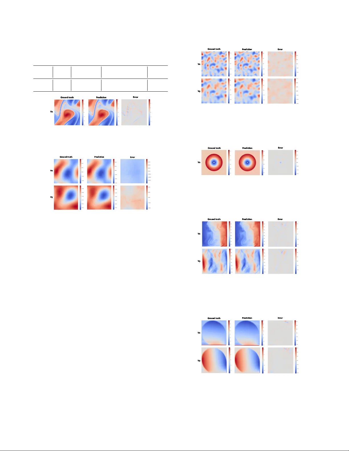
NEST OR: A Nested MOE-based Neural Operator f or Large-Scale PDE Pr e-T raining Dengdi Sun 1 , Xiaoya Zhou 1 , Xiao W ang 2 * , Hao Si 2 , W anli L yu 2 , Jin T ang 2 , Bin Luo 2 1 School of Artificial Intelligence, Anhui Uni versity , Hefei, China 2 School of Computer Science and T echnology , Anhui Uni versity , Hefei, China https://github.com/Event- AHU/OpenFusion Abstract Neural operators have emer ged as an efficient paradigm for solving PDEs, over coming the limitations of traditional nu- merical methods and significantly impr oving computational efficiency . However , due to the diversity and complexity of PDE systems, existing neural operators typically r ely on a single network arc hitecture , which limits their capacity to fully capture hetero geneous features and comple x sys- tem dependencies. This constraint poses a bottleneck for lar ge-scale PDE pr e-training based on neur al operators. T o addr ess these challenges, we pr opose a lar ge-scale PDE pr e-trained neural operator based on a nested Mixtur e-of- Experts (MoE) framework. In particular , the image-le vel MoE is designed to captur e global dependencies, while the token-level Sub-MoE focuses on local dependencies. Our model can selectively activate the most suitable e xpert net- works for a given input, ther eby enhancing g eneralization and transferability . W e conduct large-scale pr e-training on twelve PDE datasets fr om diverse sour ces and successfully transfer the model to downstream tasks. Extensive experi- ments demonstrate the ef fectiveness of our approac h. 1. Introduction Partial differential equations (PDEs) have broad applica- tions in science and engineering, including physics and fluid mechanics [ 14 ] [ 4 ] [ 33 ] [ 14 ]. Existing studies can be roughly divided into two categories: traditional numer- ical methods and data-driven methods. T raditional meth- ods, such as FEM [ 22 ] and FDM [ 16 ], approximate PDE solutions by discretizing the spatial domain, resulting in complex procedures and high computational costs. Neu- ral operators aim to learn infinite-dimensional mappings be- tween function spaces, enabling fast inference while main- taining reasonable accuracy , significantly reducing com- putational costs, and overcoming the limitations of tradi- * Corresponding Author: Xiao W ang (xiao wang@ahu.edu.cn) R o u ter ... (b) O ur Nested M oE Network Route r T ok e n E xp e r t 1 T ok e n E xp e r t n ... Image E xp e rt 1 Route r T ok e n E xp e r t 1 T ok e n E xp e r t n ... Image E xp e rt n R o u ter ... (b) O ur Nested M oE Network Route r T ok e n E xp e r t 1 T ok e n E xp e r t n ... Image E xp e rt 1 Route r T ok e n E xp e r t 1 T ok e n E xp e r t n ... Image E xp e rt n Ro ut er ... Ro u ter Exp e r t 1 Exp e r t n . . . Exp er t 1 Ro u ter Exp e r t 1 Exp e r t n . . . Exp er t 1 Ro u ter Exp e r t 1 Exp e r t n . . . Exp er t n Ro ut er ... Ro u ter Exp e r t 1 Exp e r t n . . . Exp er t 1 Ro u ter Exp e r t 1 Exp e r t n . . . Exp er t n (a) Sing le Netw o r k (b ) O ur Nest ed Mo E Ne twork (b ) O ur H iera rchic a l MoE N etwork Divers i ty & Complexity of PDE Data Sin gl e N e twork Im age L eve l Exp er t for PDEs' Divers i ty Tok en Level Exp er t for PDEs' Complexity Nested MoE Network Outp u ts (a) Sin gl e N e twork (a) Sin gl e N e twork R o u ter ... (b) O ur Nested M oE Network Route r T ok e n E xp e r t 1 T ok e n E xp e r t n ... Image E xp e rt 1 Route r T ok e n E xp e r t 1 T ok e n E xp e r t n ... Image E xp e rt n R o u ter ... (b) O ur Nested M oE Network Route r T ok e n E xp e r t 1 T ok e n E xp e r t n ... Image E xp e rt 1 Route r T ok e n E xp e r t 1 T ok e n E xp e r t n ... Image E xp e rt n Ro ut er ... Ro u ter Exp e r t 1 Exp e r t n . . . Exp er t 1 Ro u ter Exp e r t 1 Exp e r t n . . . Exp er t 1 Ro u ter Exp e r t 1 Exp e r t n . . . Exp er t n Ro ut er ... Ro u ter Exp e r t 1 Exp e r t n . . . Exp er t 1 Ro u ter Exp e r t 1 Exp e r t n . . . Exp er t n (a) Sing le Netw o r k (b ) O ur Nest ed Mo E Ne twork (b ) O ur H iera rchic a l MoE N etwork Divers i ty & Complexity of PDE Data Sin gl e N e twork Im age L eve l Exp er t for PDEs' Divers i ty Tok en Level Exp er t for PDEs' Complexity Nested MoE Network Outp u ts (a) Sin gl e N e twork (a) Sin gl e N e twork Figure 1. Comparison of two dif ferent network architectures. (a) T raditional single-netw ork architecture; (b) our proposed nested MoE architecture, where image-lev el MoE experts learn global di- versity across different PDE types, while tok en-lev el Sub-MoE e x- perts capture complex local features within equations. tional methods [ 17 ][ 24 ]. Howe ver , neural operators typi- cally rely on lar ge amounts of training data, which are often obtained through costly e xperiments and numerical simula- tions, sev erely limiting their application in wider scenarios. Recently , large-scale pre-training [ 1 ] offers a new re- search paradigm to address this problem. Unlike traditional methods, it in volves initially training models on large-scale datasets, enabling them to acquire generalizable kno wledge across dif ferent PDEs and tasks, thereby establishing a uni- fied modeling frame work. For specific do wnstream tasks, only a small amount of data is required for fine-tuning to ob- tain highly accurate solutions. This paradigm not only en- hances model generalization and effecti vely mitigates o ver - fitting but also significantly reduces the training cost and time for downstream tasks. Large-scale pre-training has been widely applied in fields such as computer vision and natural language processing [ 6 ] [ 5 ], where its superior per- formance has been well validated in practice. In the field of neural operators [ 19 ] [ 18 ], research on large-scale pre-training for PDEs has begun to take shape [ 11 ]. Howe ver , PDE systems inherently exhibit highly comple x spatiotemporal dependencies and signifi- cant regional heterogeneity within physical fields. More- ov er , different types of PDEs vary substantially in their dynamical mechanisms, boundary conditions, variable di- mensions, and numerical distributions. These factors col- lectiv ely contrib ute to the diversity and complexity of PDE system data, making unified modeling extremely challeng- ing. Existing large-scale PDE neural operators typically adopt a single network architecture. Although such mod- els can extract general representations shared across dif- ferent equations, they fall short in capturing the equation- specific characteristics of each PDE type and the localized regional correlations within a single PDE. As illustrated in Fig. 1 , con ventional architectures often struggle to simul- taneously handle the macroscopic variations across PDEs and the microscopic variations within the same PDE. If the model can incorporate more fine-grained inductive biases into its architecture—thereby learning both the commonali- ties among different PDEs and the unique properties of each equation, while further identifying local spatial correlations within the physical field—its generalization ability and task adaptability would be significantly enhanced. In recent years, the Mixture-of-Experts (MoE) frame- work [ 13 ] has attracted significant attention due to its ad- vantages in increasing model capacity while maintaining computational efficiency . Through the routing mecha- nism [ 13 ], MoE can dynamically select the most suitable expert network to provide specialized processing for each input, offering an ef ficient modeling approach for the pre- training of large-scale PDE neural operators. Howe ver , al- though single-layer MoE models can capture feature differ - ences between equation types, they still face limitations in modeling di versity and comple xity within physical fields of the same type of equations. T o address these challenges, we innovati vely incorpo- rate the MoE architecture into our model design, construct- ing a NEST ed MoE-based neural O perato R for large-scale PDE pre-training ( NESTOR ). Specifically , the image-lev el MoE adaptively acti v ates the most suitable e xperts through image-lev el routing to capture the global features of PDEs. W ithin each image-level expert, we introduce token-lev el Sub-MoEs, which selectiv ely acti vate the most appropri- ate experts via token-lev el routing to further capture the complex local correlations within the physical fields. This nested MoE architecture addresses the di versity and com- plexity of PDEs from both macro and micro perspecti ves. Through pre-training on large-scale PDE datasets, the ar- chitecture can successfully generalize to do wnstream tasks, providing an efficient modeling and solution frame work for complex PDE problems. The main contributions can be summarized as follo ws: • W e propose a novel nested Mixture-of-Experts architec- ture that integrates image-level MoE and token-le vel MoE within a unified framework, enabling cross-level e xpert collaboration. • W e designed an image-level routing mechanism that can adaptiv ely select the appropriate expert networks based on the global features of the data, thereby ef fectively cap- turing the complex heterogeneous features of dif ferent tasks at a global lev el. • Comprehensiv e v alidation on large-scale PDE datasets. W e apply the proposed framework to large-scale pre- training and do wnstream tasks across multiple PDE datasets, demonstrating significant advantages in cross- task generalization and transferability . 2. Related W orks 2.1. Neural Operators Neural operators are designed to learn mesh-free, function- space-to-function-space infinite-dimensional mappings from inputs to solution functions [ 19 ]. They effecti vely ov ercome the dependence of traditional numerical solvers on mesh discretization, impro ving computational speed and reducing costs. Moreover , for repeated problems, a neural operator only needs to be trained once, without retraining for each new PDE instance, making it an efficient paradigm for PDE solving. T o successfully apply neural operators to PDE problems, researchers have proposed several ef fecti ve model architectures. F or example, DeepONet [ 19 ] adopts a branch–trunk architecture to realize operator learning. The F ourier Neural Operator (FNO) [ 18 ] leverages Fourier transforms to capture non-local dependencies, thus enabling efficient PDE solutions. The Galerkin Transformer [ 2 ] integrates self-attention mechanisms with Galerkin pro- jection for operator learning. GNO T [ 10 ] combines graph neural operators with T ransformers, achie ving ef ficient modeling on irregular meshes. MPP [ 21 ] is a T ransformer- based autoregressi ve pre-training architecture. DPOT [ 11 ] employs autoregressi ve denoising pre-training combined with Fourier attention to predict a wide range of PDE problems. Poseidon [ 12 ] integrates neural operators with hybrid attention mechanisms to enable ef ficient and unified modeling of di verse PDEs. VIT O [ 23 ] integrates V ision T ransformers with neural operator principles, enabling vision-based PDE solving and physical field modeling. Unisolver [ 34 ] employs a PDE-conditional T ransformer architecture to achiev e unified solving across di verse PDEs, advancing tow ard univ ersal neural PDE solvers. Despite the significant progress made by neural operators, their performance still has room for improv ement due to the limitations imposed by the div ersity of data and tasks. 2.2. Mixture of Experts The Mixture of Experts (MoE) framework is a method that expands model capacity while av oiding a significant in- crease in computational cost. Its core idea is to select a subset of experts among multiple expert networks through a gating mechanism [ 13 ]. W ith the dev elopment of MoE, it has been widely applied in natural language processing, computer vision, and other domains. GShard [ 15 ] was the first to introduce the MoE structure into T ransformer models, enabling efficient large-scale distributed training. Switch Transformer [ 7 ] scaled large language model param- eters to the trillion lev el, significantly improving both model capacity and efficienc y . V -MoE [ 27 ] applied MoE to vision T ransformers and demonstrated its potential for enhancing efficienc y and performance in tasks such as image recogni- tion. Existing work primarily focuses on homogeneous e x- perts, while research on heterogeneous [ 31 ] e xperts is rel- ativ ely limited. Homogeneous experts refer to all e xperts using the same network architecture, which offers simplic- ity in implementation, stable con ver gence, and ease of load balancing. Howe ver , ha ving identical architectures limits expert di versity and, to some extent, constrains the perfor- mance of MoE. Heterogeneous e xpert MoE allo ws dif fer- ent experts to adopt dif ferent network architectures, avoid- ing redundanc y in the features learned by the experts and significantly enhancing the model’ s expressi ve po wer and efficienc y . 2.3. Pre-training Pre-training [ 1 ] refers to the process of training a model on large-scale datasets to learn general kno wledge that can be transferred to a variety of downstream tasks. It can significantly reduce the training cost of downstream tasks while improving generalizability . The pre-training paradigm has achie ved outstanding success in natural lan- guage processing, demonstrating strong cross-task transfer- ability , as e xemplified by models such as BER T [ 5 ] and GPT [ 25 ]. In computer vision, pre-training has also been widely adopted, with notable examples including the V i- sion Transformer (V iT) [ 6 ] and CLIP [ 26 ]. With the de- velopment of large-scale pre-training models, this approach has gradually been introduced into the field of PDE neural operators. Existing explorations include MPP [ 21 ], which proposes a T ransformer-based autoregressiv e pre-training framew ork capable of learning unified serialized represen- tations across various PDE datasets and allo wing cross-task modeling through transfer . DPO T [ 11 ] employs an autore- gressiv e denoising strategy combined with Fourier atten- tion to achieve efficient pre-training across multiple types of PDE problems, demonstrating cross-equation general- ization at the operator le vel. Although these studies ha ve successfully applied pre-training techniques to PDE neural operators, they still exhibit notable limitations in compre- hensiv ely capturing PDE systems. Therefore, there remains substantial room for further exploration of large-scale pre- training in the PDE neural operator domain. 3. Preliminaries In this paper, we consider the general form of a parame- terized partial differential equation defined on the spatial region Ω ⊂ R n and the time interval [0 , T ] , ∂ u ∂ t − F  u, ∇ u, ∇ 2 u, . . . ; θ  = 0 , (1) ( u ( x, 0) = u 0 ( x ) , x ∈ Ω , B [ u ]( x, t ) = g ( x, t ) , ( x, t ) ∈ ∂ Ω × (0 , T ] , where u is the unkno wn solution function, representing the state of the system; F is the PDE spatial deri vati ve operator , which describes the dynamics or ev olution law of the sys- tem and depends on the current solution u, its spatial deriv a- tiv e, and parameter θ ; θ is the external condition or physical parameter that controls the properties of the equation; u(x,0) is the initial condition; B [ u ]( x, t ) is the boundary condition. On this basis, we define a solution operator F and con- struct the following mapping F : u t +1 = F T ( u t − T +1: t ; θ ) , (2) where θ represents the system parameters. The operator F can take the most recent T frames as input and learn to im- plicitly infer the details of partial dif ferential equations, the parameters θ , to predict the next frame from the preceding T frames, thereby achie ving e volutionary prediction for dif- ferent system states. T o enhance the model’ s robustness and generalization, we inject small-scale noise into the input frames. This pretraining strategy has been sho wn to be effecti ve in DPO T [ 11 ]. 4. Proposed Method W e propose a nested MoE frame work (NESTOR), as sho wn in Fig. 2 . First, the PDE input is mapped to a latent repre- sentation space [ 11 ]. Then, these representations are input into nested MoE modules, and a gating mechanism assigns them to dif ferent experts, each capable of learning specific features of the input. The proposed network architecture in- tegrates frequency domain features and spatiotemporal fea- tures, addressing the div ersity and complexity of PDEs at both the image and token levels, thus demonstrating strong robustness and generalization ability . 4.1. Spatio-T emporal Encoding First, the input x ∈ R B × C × H × W is di vided into a set of non-ov erlapping patches X p ∈ R B × N × C × P H × P W , where B is the batch size, N is the number of patches, and ( P H × P W ) is the patch size. Each patch is then projected into a D -dimensional space, followed by the addition of positional encoding E pos [ 6 ]: X = Embedding ( X p ) + E pos ∈ R B × N × D , (3) To p - kr F l a s hA t tn - 1 1 F l a s hA t tn - 1 1 F l a s hA t tn - 1 0 F l a s hA t tn - 1 0 F l a s hA t tn - 1 2 F l a s hA t tn - 1 2 F l a s hA t tn - 1 n F l a s hA t tn - 1 n A F N O A F N O To p - kr M LP - 1 1 M LP - 1 1 M LP - 1 0 M LP - 1 0 M LP - 1 2 M LP - 1 2 M LP - 1 n M LP - 1 n Sha red M LP Sha red M LP To p - kr F l a s hA t tn - 1 1 F l a s hA t tn - 1 0 F l a s hA t tn - 1 2 F l a s hA t tn - 1 n A F N O To p - kr M LP - 1 1 M LP - 1 0 M LP - 1 2 M LP - 1 n Sha red M LP To p - kr F l a s hA t tn - 1 1 F l a s hA t tn - 1 1 F l a s hA t tn - 1 0 F l a s hA t tn - 1 0 F l a s hA t tn - 1 2 F l a s hA t tn - 1 2 F l a s hA t tn - 1 n F l a s hA t tn - 1 n A F N O A F N O To p - kr M LP - 1 1 M LP - 1 1 M LP - 1 0 M LP - 1 0 M LP - 1 2 M LP - 1 2 M LP - 1 n M LP - 1 n Sha red M LP Sha red M LP To p - kr F l a s hA t tn - 1 1 F l a s hA t tn - 1 0 F l a s hA t tn - 1 2 F l a s hA t tn - 1 n A F N O To p - kr M LP - 1 1 M LP - 1 0 M LP - 1 2 M LP - 1 n Sha red M LP Figure 2. Overview architecture. W e train on twelve mixed PDE datasets, predicting the next frame based on the preceding frames. W e design a nested MoE architecture: (1) the top shows the overall model architecture; (2) the bottom right illustrates the nested Sub-MoE architecture; and (3) the bottom left depicts the improv ed Flash Attention architecture. Subsequently , the obtained representation is rearranged as X ∈ R B × X × Y × T × C , and mapping time series to a fix ed dimension to compress information in the time dimension: Y = T X t =1 W t X t , Y ∈ R B × X × Y × C out , (4) where W ∈ R T × C out × C out is a learnable weight matrix. 4.2. Nested Mixture-of-Experts Ar chitecture A single type of network architecture is insuf ficient to fully capture the div erse characteristics of data. T o address this, we introduce a nested MoE architecture at the operator level to enable multi-scale interactions within the PDE system. This module dynamically allocates the most appropriate e x- pert network through a routing me chanism, allowing it to si- multaneously characterize both local and global dependen- cies and effecti vely capture features in both the time and frequency domains. Here, both the image-le vel MoE and the token-lev el Sub-MoE consist of 6 non-shared experts and 1 shared e xpert, with the gating network acti vating 2 of the non-shared experts. 4.2.1. Image-level MoE Routing Strategy . W e adopt an image-lev el gating mecha- nism and employ a top-k routing strategy [ 28 ] for expert se- lection. First, giv en the input feature x ∈ R B × C × H × W , we apply global average pooling to obtain the image-le vel rep- resentation ¯ x b ∈ R C , where b = 1 , . . . , B . Next, the image- lev el representation is fed into a learnable linear layer to produce the raw e xpert scores: s b = ¯ x b W ⊤ + b ∈ R N , (5) where W ∈ R N × C is the expert weight matrix, b ∈ R N is the bias term, and N denotes the number of experts. The raw scores are then normalized using the softmax to obtain the routing probabilities p b = softmax ( s b ) , N X i =1 p b,i = 1 . (6) Finally , according to the top- k routing strategy , the k ex- perts with the highest probabilities are selected. Let I b de- note the index set of the selected experts. For each selected expert i ∈ I b , the final routing weight is defined as: w b,i = p b,i P j ∈I b pb, j , i ∈ I b . (7) Expert Design. W e select AFNO [ 8 ] [ 11 ] as the shared expert, responsible for capturing global low-frequenc y spa- tial features. First, the input feature x ∈ R B × C × H × W is F ourier transformed: ˆ x = F ( x ) , ˆ x ∈ C B × H × W × C , where F ( · ) is the FFT operation. Next, a complex con v olu- tion operation is performed in the frequency domain: ˆ y real = σ  ˆ x real W ( r ) 1 − ˆ x imag W ( i ) 1 + b ( r ) 1  , (8) ˆ y imag = σ  ˆ x imag W ( r ) 1 + ˆ x real W ( i ) 1 + b ( i ) 1  , (9) where σ is the acti vation function, W ( r ) 1 , W ( i ) 1 are learnable matrices for the real and imaginary parts, respectiv ely , and b ( r ) 1 , b ( i ) 1 are bias terms. Then, an in verse Fourier transform is performed to return to the spatiotemporal representation: y = F − 1 ( ˆ y ) , (10) where F − 1 ( · ) represents the IFFT operation. Finally , a nor - malization layer , MLP , and residual connections are com- bined to obtain the output of the shared expert. In addition, we introduce Flash Attention [ 3 ] as a non- shared expert, responsible for capturing the fine-grained spatiotemporal features of the physical field. First, the input feature x ∈ R B × C × H × W is reshaped into a sequence form x ′ ∈ R B × C × N , where N = H × W . Ne xt, x ′ is normal- ized and linearly transformed to obtain the query ( Q ), key ( K ), and v alue ( V ) representations. The attention-weighted result is then computed as Z = softmax  QK ⊤ √ d k  V , which is added to the input residual and further normalized to obtain ˜ Z . Subsequently , ˜ Z is passed through a Sub-MoE module for linear transformation: Y = Sub-MoE ( ˜ Z ) . (11) Finally , by combining residual connections and normaliza- tion layers, we obtain the output of the non-shared expert. 4.2.2. T oken-level Sub-MoE Routing Strategy . W e adopt a token-le vel gating mecha- nism and employ a top-k routing strategy for expert selec- tion. Unlike the image-lev el gating mechanism, the token- lev el gates e xpert scores for each individual token vector , enabling finer-grained e xpert selection. Expert Design. Our Sub-MoE implements the functional- ity of the FFN layer in Flash Attention. Both the shared and non-shared experts adopt the same netw ork structure, which is an MLP . Normalized features are fed into the Sub-MoE, where token-lev el routing assigns them to the most appro- priate e xpert for processing, extracting fine-grained feature representations. The computational process is as follows. ExpertMLP ( x ) = W 2 σ ( W 1 x + b 1 ) + b 2 , (12) where W 1 ∈ R C × ( rC ) , W 2 ∈ R ( rC ) × C , r is mlp ratio, σ ( · ) denotes the activ ation function of GELU. Specifically , we first perform the first-layer linear transformation on the input feature h = xW 1 + b 1 . Next, perform a nonlinear activ ation on h : a = GELU ( h ) . Finally , a second linear transformation is performed to obtain the final feature rep- resentation: y = aW 2 + b 2 . 4.3. Head and Loss Function 4.3.1. Load Balancing Loss In our nested MoE model, the routing mechanism assigns tokens to the most suitable experts. A balanced distribu- tion of tokens among e xperts is crucial for MoE perfor- mance. When the allocation is imbalanced, some experts remain idle and fail to learn diverse features, while a few ex- perts become o verloaded, potentially causing memory bot- tlenecks. This can lead the model to de generate to using only a subset of experts, failing to fully le verage the adv an- tages of MoE [ 29 ]. T o address this issue, we introduce a load-balancing loss [ 28 ] to encourage a more uniform dis- tribution of tokens across experts. Here, the two load bal- ancing losses are defined following the same pattern: L aux = E E X i =1 p i · f i , (13) where p i = 1 N P N j =1 P ij is the routing probability of ex- pert i , f i = n i P E k =1 n k is the actual token assignment ratio of expert i , E is the total number of experts, N is the total number of tok ens, P ij is the probability of token j being assigned to expert i , and n i denotes the number of tok ens assigned to expert i . 4.3.2. Main T ask Loss For our prediction task, we choose the relati ve error (L2RE) [ 18 ] as the main task loss function: L 2 =    ˆ y ( c ) i − y ( c ) i    2    y ( c ) i    2 , (14) where y ( c ) i is the ground-truth of i -th sample at channel c , and ˆ y ( c ) i is the corresponding prediction. 4.3.3. T otal Loss Ultimately , our loss function consists of the main task loss and two load-balancing losses: L = L 2 + α L aux 1 + β L aux 2 , (15) where L 2 denotes the main task’ s L2RE; L aux 1 is the load balancing loss of Image-le vel MoE (image-lev el routing); L aux 2 is the load balancing loss of the Image-level Sub- MoE (token-le vel routing); and α and β are hyperparam- eters that control the contribution of the load balancing losses. 5. Experiments 5.1. Datasets and Evaluation Metric Datasets. W e conduct e xperiments on a mixed dataset con- sisting of twelve dif ferent data sources and different pa- rameters from FNO [ 18 ], PDEBench [ 30 ], PDEArena [ 9 ], and CFDBench [ 20 ]. (1) FNO: A dataset containing three different parameters for the same type of equation. (2) PDEBench: A dataset containing four different parameters for the same type of equation. (3) PDEArena: A dataset containing the same equation with and without initial con- ditions. (4) CFDBench: A multi-task PDE dataset obtained by processing the four subtasks uniformly . Evaluation Metrics. W e use L2RE [ 18 ] as the ev aluation metric, where lower L2RE indicates better performance. T able 1. The experiments are divided into two parts: one reports the pre-training performance of the model, and the other shows the fine-tuning results on each task. Here, “-200” denotes fine-tuning for 200 epochs, and “-500” for 500 epochs. The ev aluation metric is L2RE. The best result within each part is highlighted in bold , while the ov erall best result is emphasized in blue bold. L2RE Activ ated FNO- ν PDEBench CNS-( η, ζ ), DR, SWE PDEArena CFDBench Model Params 1e-5 1e-4 1e-3 1,0.1 1,0.01 A vg.(1) 0.1,0.1 0.1,0.01 Avg.(0.1) DR SWE NS NS-cond - Pre-trained FNO 0.5M 0.116 0.0922 0.0156 0.151 0.108 0.130 0.230 0.076 0.153 0.0321 0.0091 0.210 0.384 0.0274 UNet 25M 0.198 0.119 0.0245 0.334 0.291 0.313 0.569 0.357 0.463 0.0971 0.0521 0.102 0.337 0.209 FFNO 1.3M 0.121 0.0503 0.0099 0.0212 0.052 0.0366 0.162 0.0452 0.104 0.0571 0.0116 0.0839 0.602 0.0071 GK-T 1.6M 0.134 0.0792 0.0098 0.0341 0.0377 0.0359 0.0274 0.0366 0.0320 0.0359 0.0069 0.0952 0.423 0.0105 GNOT 1.8M 0.157 0.0443 0.0125 0.0325 0.0420 0.0373 0.0228 0.0341 0.0285 0.0311 0.0068 0.172 0.325 0.0088 Oformer 1.9M 0.1705 0.0645 0.0104 0.0417 0.0625 0.0521 0.0254 0.0205 0.0229 0.0192 0.0072 0.135 0.332 0.0102 MPP-T 7M - - - - - 0.0442 - - 0.0312 0.0168 0.0066 - - - DPOT -T 7M 0.0976 0.0606 0.00954 0.0173 0.0397 0.0285 0.0132 0.0220 0.0176 0.0321 0.0056 0.125 0.384 0.0095 Ours 13M 0.1195 0.0951 0.0093 0.0167 0.0373 0.0270 0.0120 0.0202 0.0161 0.0308 0.0052 0.132 0.409 0.0112 Fine-tune DPOT -FT200 7M 0.0511 0.0431 0.0073 0.0136 0.0238 0.0187 0.0168 0.0145 0.0157 0.0194 0.0028 0.103 0.313 0.0054 Ours -FT200 13M 0.0581 0.0313 0.0056 0.0139 0.0182 0.0161 0.0155 0.0112 0.0134 0.0198 0.0032 0.0793 0.321 0.0045 DPOT -FT500 7M 0.0520 0.0367 0.0058 0.0112 0.0195 0.0153 0.0174 0.0138 0.0156 0.0148 0.0024 0.0910 0.280 0.0039 Ours -FT500 13M 0.0505 0.0217 0.0043 0.0094 0.0134 0.0114 0.0123 0.0083 0.0103 0.0117 0.0026 0.0683 0.285 0.0038 5.2. Main Results T able 1 presents the e xperimental results of our method compared with other models in the pre-training datasets. The first ro w of the table specifies the types of PDE datasets and parameter settings, while the first column lists the base- line models for comparison. The experiments are di vided into two parts: the first is pre-training, where all models are trained from scratch on the datasets; the second is fine- tuning, where models are further trained based on the pre- trained weights. In the pre-training stage, our method demonstrates strong performance across 12 PDE datasets, achie ving state-of-the-art results on 6 of them. Notably , our model ranks first on 5 out of 6 PDEBench datasets, and achiev es significantly lo wer errors than mainstream models on mul- tiple benchmarks. These results clearly validate the effec- tiv eness of our proposed architecture for handling comple x PDE systems, highlighting its superior performance and generalizability in PDE modeling. In the fine-tuning stage, we conduct 200 and 500 epochs of fine-tuning on each dataset. The results show that af- ter 500 epochs, our model achieves state-of-the-art perfor- mance on 9 out of 12 tasks, surpassing advanced pre-trained models on the majority of tasks. Compared with train- ing from scratch, fine-tuning on pretrained weights gener - ally leads to better performance; moreov er, increasing the number of fine-tuning steps typically yields higher predic- tion accuracy . These results demonstrate the superior per- formance of our proposed model on sparse datasets with stronger generalization and adaptability . In summary , our model demonstrates significant advan- tages in operator learning for PDE tasks. W ith the aid of fine-tuning strategies, it can rapidly adapt to specific tasks and achiev e a total of 10 global best performances across 12 benchmark datasets, highlighting its strong modeling capa- bility in capturing complex dynamics and multi-scale fea- tures, as well as its excellent generalization ability . Vy Vx Density Pressure Ground t ruth Predic tion Error Ground t ruth Predic tion Error Vy Vx Density Pressure Ground t ruth Predic tion Error Ground t ruth Predic tion Error Figure 3. V isualization of 2D high-resolution turbulence predic- tion results. (1) The first column sho ws the true v alues, the second shows the model predictions, and the third shows the correspond- ing errors. (2) The predicted ph ysical quantities are horizontal velocity , v ertical velocity , density field, and pressure field. T u r b u l e n c e ( G e o - ) F N O 0 . 1 9 3 M P P - F T 0 . 1 5 2 D P O T - V a n i l l a 0 . 1 6 7 D P O T - F T 0 . 1 3 5 O u r s - V a n i l l a 0 . 1 8 2 2 O u r s - F T 0 . 0 7 1 1 Figure 4. Performance comparison of dif ferent models on the 2D high-resolution turbulence task. W e use L2RE as the evaluation metric, where V anilla denotes training from scratch, and -FT indi- cates results after 500 fine-tuning epochs on the downstream task. 5.3. Downstr eam T asks Experiments T o ev aluate the generalization and transferability of our model, we conduct downstream experiments on a two- dimensional high-resolution turbulence task ( 512 × 512 ). In these experiments, we reuse most of the parameters from T able 2. The impact of the number of non-shared experts. W e use L2RE as the ev aluation metric. Setting Num. of experts FNO PDEBench SWE A vg. L 2 FT -200 2 0.0575 0.0182 0.0024 0.0262 4 0.0577 0.0240 0.0579 0.0466 6 0.0563 0.0150 0.0025 0.0246 12 0.0575 0.1896 0.0025 0.0832 FT -500 2 0.0519 0.0126 0.0022 0.0222 4 0.0504 0.0114 0.0025 0.0214 6 0.0502 0.0115 0.0021 0.0213 12 0.0520 0.0144 0.0025 0.0230 T able 3. The impact of the size of the pre-training data on perfor- mance. W e use L2RE as the evaluation metric. Num. of datasets FNO PDEBench SWE A vg. L 2 3 0.0512 0.0165 0.0026 0.0234 12 0.0505 0.0094 0.0026 0.0208 the pre-trained model, including the weights of the MoE modules and the spatio-temporal encoding. The visualiza- tion of the model predictions is shown in Fig. 3 . As illustrated in Fig. 4 , most models fine-tuned from pre-trained weights outperform those trained from scratch, which demonstrates the effecti veness of large-scale pre- training. This indicates that the model can acquire gen- eralizable PDE kno wledge and successfully transfer it to specific downstream tasks. On the two-dimensional high- resolution turbulence task, our model achie ves a 47.3 % im- prov ement in prediction accuracy , reaching the best perfor- mance. The experimental results demonstrate that our pre- trained model learns more ef fective representations, achiev- ing strong transfer performance on downstream tasks with only minimal fine-tuning. Moreover , it maintains precise prediction capability e ven on high-resolution tasks, fully showcasing its adv antage in capturing PDE characteristics. 5.4. Scaling Experiments The number of experts in the MoE architecture is a k ey factor influencing the performance of pre-trained models. Under the setting where the number of acti vated experts per forward pass is fixed, we vary the number of unshared experts and use the average L2RE across datasets as the ev aluation metric to study how the number of non-shared experts af fects pre-training performance. On the selected datasets, we adopt two fine-tuning strategies: FT -200 (200 steps of fine-tuning) and FT -500 (500 steps of fine-tuning). As shown in T able 2 , the results indicate that fine-tuning the pre-trained model significantly improves task performance, and additional fine-tuning steps lead to further gains. F or complex MoE architectures, howe ver , having more experts is not always better; increasing the number of experts makes optimization more challenging and complicates resource al- T able 4. Ablation e xperiments of our proposed model on the PDEBench datasets. “w/o” denotes the removal of the correspond- ing component. W e use L2RE as the evaluation metric. Method 1,0.1 1,0.01 0.1,0.1 0.1,0.01 DR SWE A vg. L 2 Promotion Ours 0.0144 0.0355 0.0135 0.0178 0.0282 0.0045 0.0173 - w/o Sub-MoE 0.0157 0.0393 0.0130 0.0209 0.0245 0.0049 0.0197 0.0024 w/o Load Balance Loss 0.0135 0.0335 0.0109 0.0159 0.0265 0.0062 0.0178 0.0005 FlashAttn + AFNO Sum 0.0149 0.0363 0.0136 0.0178 0.0304 0.0046 0.0196 0.0023 location. For dif ferent tasks, there typically exists an opti- mal range for the number of experts, and selecting an ap- propriate expert size is essential for fully realizing the per - formance potential of MoE models. W e in vestigate the impact of pre-training data scale on model performance, as sho wn in T able 3 . Specifically , we conduct pre-training on 3 and 12 different PDE datasets, followed by 500 epochs of fine-tuning on each downstream task. The results demonstrate that increasing the amount of pre-training data improves fine-tuning performance, in- dicating that large-scale cross-equation pre-training effec- tiv ely enhances the model’ s generalization capability . 5.5. Ablation Studies T o validate the ef fecti veness of our model, we conduct ex- periments on six sub-tasks of the PDEBench dataset to as- sess the impact of dif ferent modules on model performance. Using the complete model as the baseline, we systemati- cally perform ablation studies by progressi vely removing or replacing key modules, with the average L2RE (A vg. L 2 ) serving as the primary comprehensiv e ev aluation met- ric. The results are shown in T able 4 . Impact of Sub-MoE. Removing the Sub-MoE module leads to an increase of 0.0024 in the a verage L2RE. Among all modules, Sub-MoE contributed most significantly to per- formance improv ement, indicating that it plays an impor- tant role in effecti vely capturing multi-scale and div erse fea- tures, thereby fully validating its importance. Impact of the Load Balancing Loss. Removing the load balancing loss results in an increase of 0.0005 in the aver - age L2RE. Although its contrib ution is smaller compared to other modules, it still provides a certain improvement to model performance. Impact of the Fusion Strategy . Changing the fusion of AFNO and FlashAttention from MoE to simple addition in- creases the A vg. L2RE by 0.0023. This demonstrates that our model can select the most suitable experts for different inputs, thereby enhancing model performance and general- ization ability , and v alidates the rationality of the design. 5.6. Interpr etable Analysis T o verify the effecti veness of the proposed nested MoE (Mixture of Experts) architecture, we conduct experiments at two levels: the global feature modeling capability of image-lev el experts and the local region modeling capabil- Exp ert 0 Exp ert 1 Exp ert 2 Exp ert 3 Exp ert 4 Exp ert 5 F NO CFD NS Exp ert 0 Exp ert 1 Exp ert 2 Exp ert 3 Exp ert 4 Exp ert 5 F NO CFD NS Figure 5. V isualization of spatial activation patterns produced by token-le vel experts in the Sub-MoE layer . F or each input sample, the expert acti vation probabilities are projected onto heatmaps. ity of token-le vel experts. Effectiveness of Image-Level MoE. The image-level gat- ing network generates expert scores based on the global features of the input samples and activ ates the two experts with the highest scores through a T op-2 selection mecha- nism. W e statistically analyze the activ ation frequency of each expert on different PDE-type datasets to examine the correlation between e xpert selection and equation type. The results are sho wn in T able 5 . It can be seen that Expert 0 and Expert 1 show a significant preference in the NS2D (Navier–Stok es) dataset, with a combined acti vation rate exceeding 70%, indicating that these two e xperts are adept at handling complex flow characteristics dominated by con- vection. Expert 2 and Expert 3 dominate activ ation on the SWE (Shallow W ater W a ve Equation) dataset, with a com- bined activ ation frequency of 99.74%, demonstrating their ability to model the characteristics of wave propagation pro- cesses. Expert 0 and Expert 5 perform outstandingly in the DR (Diffusion–Reaction) dataset, with a combined activ a- tion rate of 78.77%, indicating their ability to capture the chemical reaction source term and diffusion-flo w coupling effect in the diffusion process. In the two similar equation datasets with different parameters, M1(-1,-1) and M-1(-1,- 1), Expert 0 and Expert 1 are also frequently selected, in- dicating that image-level MoE can effecti vely distinguish PDE types and select the optimal expert combination. Ex- perimental results show that image-le vel e xperts can adap- tiv ely identify global features of different PDE types and automatically select the most suitable expert combination for modeling through a gating mechanism. Effectiveness of T oken-Level MoE. T o v erify the spatial region modeling capability of token-lev el experts, we con- duct a visualization experiment based on spatial heatmaps. For each input sample, the activ ation probabilities of token- lev el experts are extracted from the Sub-MoE layer , gen- erating a heatmap, as shown in Fig. 5 . The visualization results sho w that different token-lev el experts exhibit dis- tinct region-specific activ ation patterns in space. This pat- tern indicates that token-le vel MoE can effecti vely capture local region correlations within the physical field, providing T able 5. Expert selection distribution of the MoE router across different datasets. The top two experts for each dataset are high- lighted in bold (%). Dataset Expert 0 Expert 1 Expert 2 Expert 3 Expert 4 Expert 5 M1(-1,-1) 22.39 50.00 6.98 5.37 10.69 4.58 M-1(-1,-1) 22.88 50.00 3.51 11.58 10.22 1.81 SWE 0.00 0.00 50.00 49.74 0.00 0.25 DR 28.77 0.00 2.31 12.64 6.28 50.00 T able 6. Comparison of activ ation parameters, total parameters, and activ ation rates of different models. DPO T -T MoE-PO T -T Ours Activ ated Parameters 7.5M 17M 13M T otal Parameters 7.5M 30M 83M Activ ation Ratio 100% 56.67% 16.67% a more refined expressi ve capability for modeling complex multi-scale physical systems. In summary , our nested MoE architecture is effecti ve. At the macroscopic le vel, image-lev el experts achieve adap- tiv e functional division based on PDE types; at the mi- croscopic le vel, token-lev el experts effecti vely capture re- gional correlations within the physical field. This dual spe- cialization mechanism of ”macroscopic classification – mi- croscopic partitioning” significantly improv es the model’ s modeling and generalization capabilities for complex mul- tiphysics problems. 5.7. Efficiency Analysis W e analyze the efficiency of our models, as shown in T a- ble 6 . Traditional single-network architectures, such as DPO T -T , can only increase model capacity by adding more parameters, which typically leads to a linear growth in computational cost. In contrast, models incorporating the Mixture-of-Experts (MoE) mechanism, such as MoE-PO T - T [ 32 ] and Ours, can expand model capacity through selec- tiv e activ ation of expert sub-networks, thereby improving performance while keeping computational costs lo w . Specifically , although ours has a much larger total num- ber of parameters compared to DPO T -T and MoE-PO T -T , its activ ated parameter ratio is only 16.67%, significantly lower than MoE-PO T -T’ s 56.67% and DPO T -T’ s 100%. This demonstrates that the selective acti v ation of MoE not only allows the model to achiev e higher capacity without in- creasing the actual computational burden b ut also provides a practical solution for efficient scaling. 6. Conclusion This paper proposes a large-scale PDE pre-trained neural operator based on a nested Mixture-of-Experts (MoE) ar- chitecture. W e design the nested MoE framework, which consists of image-level MoE and token-lev el MoE, and con- duct extensi ve training on twelve PDE datasets to obtain a univ ersal pre-trained model. Our model successfully trans- fers to specific tasks and ne w downstream tasks, achie ving state-of-the-art performance on most datasets. Furthermore, this paper explores the suitability and advantages of MoE architectures for large-scale PDE pre-trained neural opera- tors, pioneers the design of a hierarchical MoE architecture in this field, and rev eals new potential for solving PDEs. References [1] Y oshua Bengio. Deep learning of representations for un- supervised and transfer learning. In Proceedings of ICML workshop on unsupervised and transfer learning , pages 17– 36. JMLR W orkshop and Conference Proceedings, 2012. 1 , 3 [2] Shuhao Cao. Choose a transformer: Fourier or galerkin. Ad- vances in neur al information pr ocessing systems , 34:24924– 24940, 2021. 2 [3] T ri Dao, Dan Fu, Stefano Ermon, Atri Rudra, and Christo- pher R ´ e. Flashattention: Fast and memory-ef ficient e xact attention with io-awareness. Advances in neural information pr ocessing systems , 35:16344–16359, 2022. 5 [4] Lokenath Debnath. Nonlinear partial differ ential equations for scientists and engineers . Springer, 2005. 1 [5] Jacob Devlin, Ming-W ei Chang, Kenton Lee, and Kristina T outano v a. Bert: Pre-training of deep bidirectional trans- formers for language understanding. In Pr oceedings of the 2019 conference of the North American chapter of the asso- ciation for computational linguistics: human langua ge tec h- nologies, volume 1 (long and short papers) , pages 4171– 4186, 2019. 1 , 3 [6] Alex ey Dosovitskiy , Lucas Beyer , Alexander Kolesnik ov , Dirk W eissenborn, Xiaohua Zhai, Thomas Unterthiner, Mostafa Dehghani, Matthias Minderer, Georg Heigold, Syl- vain Gelly , et al. An image is worth 16x16 words: Trans- formers for image recognition at scale. arXiv pr eprint arXiv:2010.11929 , 2020. 1 , 3 [7] W illiam Fedus, Barret Zoph, and Noam Shazeer . Switch transformers: Scaling to trillion parameter models with sim- ple and efficient sparsity . Journal of Machine Learning Re- sear ch , 23(120):1–39, 2022. 3 [8] John Guibas, Morteza Mardani, Zongyi Li, Andrew T ao, An- ima Anandkumar, and Bryan Catanzaro. Adapti ve fourier neural operators: Efficient token mixers for transformers. arXiv pr eprint arXiv:2111.13587 , 2021. 4 [9] Jayesh K Gupta and Johannes Brandstetter . T owards multi-spatiotemporal-scale generalized pde modeling. arXiv pr eprint arXiv:2209.15616 , 2022. 5 [10] Zhongkai Hao, Zhengyi W ang, Hang Su, Chengyang Y ing, Y inpeng Dong, Songming Liu, Ze Cheng, Jian Song, and Jun Zhu. Gnot: A general neural operator transformer for operator learning. In International Confer ence on Mac hine Learning , pages 12556–12569. PMLR, 2023. 2 [11] Zhongkai Hao, Chang Su, Songming Liu, Julius Berner , Chengyang Y ing, Hang Su, Anima Anandkumar, Jian Song, and Jun Zhu. Dpot: Auto-regressi ve denoising operator transformer for large-scale pde pre-training. arXiv preprint arXiv:2403.03542 , 2024. 1 , 2 , 3 , 4 [12] Maximilian Herde, Bogdan Raonic, T obias Rohner , Roger K ¨ appeli, Roberto Molinaro, Emmanuel de B ´ ezenac, and Sid- dhartha Mishra. Poseidon: Efficient foundation models for pdes. Advances in Neural Information Pr ocessing Systems , 37:72525–72624, 2024. 2 [13] Robert A Jacobs, Michael I Jordan, Stev en J Nowlan, and Geoffre y E Hinton. Adaptiv e mixtures of local e xperts. Neu- ral computation , 3(1):79–87, 1991. 2 , 3 [14] George Em Karniadakis, Ioannis G K evrekidis, Lu Lu, P aris Perdikaris, Sifan W ang, and Liu Y ang. Physics-informed machine learning. Natur e Re views Physics , 3(6):422–440, 2021. 1 [15] Dmitry Lepikhin, HyoukJoong Lee, Y uanzhong Xu, Dehao Chen, Orhan Firat, Y anping Huang, Maxim Krikun, Noam Shazeer , and Zhifeng Chen. Gshard: Scaling giant models with conditional computation and automatic sharding. arXiv pr eprint arXiv:2006.16668 , 2020. 3 [16] Randall J LeV eque. F inite differ ence methods for ordinary and partial dif ferential equations: steady-state and time- dependent pr oblems . SIAM, 2007. 1 [17] Zongyi Li. Neural operator: Learning maps between func- tion spaces. In 2021 F all W estern Sectional Meeting . AMS, 2021. 1 [18] Zongyi Li, Nikola K ov achki, Kamyar Azizzadenesheli, Burigede Liu, Kaushik Bhattacharya, Andrew Stuart, and Anima Anandkumar . Fourier neural operator for para- metric partial dif ferential equations. arXiv pr eprint arXiv:2010.08895 , 2020. 1 , 2 , 5 [19] Lu Lu, Pengzhan Jin, and George Em Karniadakis. Deep- onet: Learning nonlinear operators for identifying differen- tial equations based on the universal approximation theorem of operators. arXiv pr eprint arXiv:1910.03193 , 2019. 1 , 2 [20] Y ining Luo, Y ingfa Chen, and Zhen Zhang. Cfdbench: A large-scale benchmark for machine learning methods in fluid dynamics. arXiv pr eprint arXiv:2310.05963 , 2023. 5 [21] Michael McCabe, Bruno R ´ egaldo-Saint Blancard, Liam Holden Parker , Ruben Ohana, Miles Cranmer, Alberto Bietti, Michael Eickenberg, Siavash Golkar , Ger- aud Krawezik, Francois Lanusse, et al. Multiple physics pretraining for physical surrogate models. arXiv preprint arXiv:2310.02994 , 2023. 2 , 3 [22] Douglas H Norrie and Gerard De Vries. The finite element method: fundamentals and applications . Academic Press, 2014. 1 [23] Oded Ov adia, Adar Kahana, P anos Stinis, Eli T urkel, Dan Gi voli, and George Em Karniadakis. V ito: V ision transformer-operator . Computer Methods in Applied Me- chanics and Engineering , 428:117109, 2024. 2 [24] Jaideep Pathak, Shashank Subramanian, Peter Harrington, Sanjeev Raja, Ashesh Chattopadhyay , Morteza Mardani, Thorsten Kurth, David Hall, Zongyi Li, Kamyar Azizzade- nesheli, et al. Fourcastnet: A global data-driv en high- resolution weather model using adaptive fourier neural op- erators. arXiv pr eprint arXiv:2202.11214 , 2022. 1 [25] Alec Radford, Karthik Narasimhan, T im Salimans, Ilya Sutske ver , et al. Improving language understanding by gen- erativ e pre-training. 2018. 3 [26] Alec Radford, Jong W ook Kim, Chris Hallacy , Aditya Ramesh, Gabriel Goh, Sandhini Agarwal, Girish Sastry , Amanda Askell, P amela Mishkin, Jack Clark, et al. Learning transferable visual models from natural language supervi- sion. In International conference on machine learning , pages 8748–8763. PmLR, 2021. 3 [27] Carlos Riquelme, Joan Puigcerver , Basil Mustafa, Maxim Neumann, Rodolphe Jenatton, Andr ´ e Susano Pinto, Daniel Ke ysers, and Neil Houlsby . Scaling vision with sparse mix- ture of experts. Advances in Neural Information Processing Systems , 34:8583–8595, 2021. 3 [28] Noam Shazeer , Azalia Mirhoseini, Krzysztof Maziarz, Andy Davis, Quoc Le, Geof frey Hinton, and Jef f Dean. Outra- geously large neural networks: The sparsely-gated mixture- of-experts layer . arXiv preprint , 2017. 4 , 5 [29] N Shazeer , A Mirhoseini, K Maziarz, A Davis, Q Le, G Hin- ton, and J Dean. The sparsely-gated mixture-of-experts layer . Outrag eously large neur al networks , 2, 2017. 5 [30] Makoto T akamoto, T imothy Praditia, Raphael Leiteritz, Daniel MacKinlay , Francesco Alesiani, Dirk Pfl ¨ uger , and Mathias Niepert. Pdebench: An extensi ve benchmark for scientific machine learning. Advances in Neural Information Pr ocessing Systems , 35:1596–1611, 2022. 5 [31] An W ang, Xingwu Sun, Ruobing Xie, Shuaipeng Li, Jiaqi Zhu, Zhen Y ang, Pinxue Zhao, JN Han, Zhanhui Kang, Di W ang, et al. Hmoe: Heterogeneous mixture of experts for language modeling. arXiv pr eprint arXiv:2408.10681 , 2024. 3 [32] Hong W ang, Haiyang Xin, Jie W ang, Xuanze Y ang, Fei Zha, Huanshuo Dong, and Y an Jiang. Mixture-of-experts operator transformer for large-scale pde pre-training. arXiv preprint arXiv:2510.25803 , 2025. 8 [33] Eleftherios C Zachmanoglou and Dale W Thoe. Intr oduction to partial differ ential equations with applications . Courier Corporation, 1986. 1 [34] Hang Zhou, Y uezhou Ma, Haixu W u, Haowen W ang, and Mingsheng Long. Unisolver: Pde-conditional transformers tow ards universal neural pde solvers. In F orty-second Inter- national Confer ence on Machine Learning . 2 A. appendix A.1. LLM USA GE During the manuscript writing and revision process, we used a Large Language Model (LLM) to assist. Specifically , LLM was used to improve the accuracy and readability of the language, and to help ensure the ov erall structure and clarity of the paper . This tool primarily assisted with tasks such as sentence reconstruction, grammatical proofreading, and improving te xt coherence. A.2. Experimental Details Pre-training . W e pre-trained the model on 8 NVIDIA R TX 4090 GPUs using the Adam optimizer with an initial learn- ing rate of 1 . 0 × 10 − 3 and a cyclic learning rate schedule (cycle), including 200 warm-up epochs. The total training lasted 1000 epochs with a batch size of 32. T o mitigate the effects of varying dataset sizes, training weights were as- signed to each dataset. During training, we used T = 10 time steps to predict the ne xt frame, maintaining consis- tency with the original settings of most datasets. The details are shown in T able 7 . Fine-tuning. In the fine-tuning stage, we loaded the pre- trained weights and performed 200-epoch and 500-epoch fine-tuning on each subset. The key module of the model is the nested MoE layer, whose parameters are shared across different frequency components along the channel dimen- sion, enabling cross-lev el expert collaboration. A.3. Data Prepr ocessing and Sampling Data Padding and Masking. Different PDE datasets vary in resolution, number of variables, and geometric configu- rations. If we directly sample from the raw data, the re- sulting batch will have large v ariations in size, leading to unbalanced training loads and reduced ef ficiency in mod- ern multi-GPU training. Here, we adopt the padding and masking strate gy from DPOT . First, we select a fixed reso- lution H = 128 , which matches a considerable portion of the datasets. Datasets with lower resolutions are upsampled to H via interpolation, while those with higher resolutions are randomly downsampled or interpolated to H . Second, to unify the number of variables across different PDEs, we pad all datasets along the channel dimension (e.g., filling with ones) to match the maximum number of channels. For datasets with irregular geometries, an additional mask chan- nel is introduced to encode the specific geometric configu- ration of each PDE instance. Balanced Data Sampling . When training with multiple PDE datasets, differences among datasets can lead to un- balanced training progress and inef ficiency . T o address this issue, we adopt the sampling strate gy from DPO T , which balances the sampling probabilities across datasets during training. Our goal is to ensure that each dataset is repre- sented equally throughout the training process. Let | D k | denote the number of samples in the k -th dataset ( 1 ≤ k ≤ K ), and assign a weight w k to each dataset to indicate its relativ e importance. Then, the sampling probability from dataset D k is defined as: p k = w k K | D k | P k w k W e can observe that the sampling probability depends on the weight w k rather than the dataset size | D k | , which helps mitigate gradient imbalance caused by dataset size dispari- ties. A.4. Limitations and Conclusions W e use DPO T as our primary baseline and adopt its data processing strate gies, including adding noise, data padding, and balanced data sampling. Howe ver , our core model dif- fers from DPO T , which is based on AFNO, while our net- work architecture employs a nested MoE. MoE-PO T , our work, also incorporates a MoE architecture, but uses only a single-layer MoE and primarily improves upon the fre- quency con volution in AFNO. In contrast, our proposed nested MoE architecture processes PDE features at both macroscopic and microscopic levels, achie ving an ef fective fusion of frequency domain and spatiotemporal domain fea- tures. Due to resource constraints, our model is currently only implemented with one parameter size, but this version has already demonstrated good accurac y and generalization ability . Combining the results of scaling experiments and interpretability analysis, we validate the model’ s effecti ve- ness and show that it can be scaled to versions with different parameter sizes. Considering the di versity of expert and ac- tiv ation numbers, future work can explore optimal parame- ter configurations to further improv e model performance. A.5. Detailed Inf ormation of Datasets W e list the configurations of the PDE datasets used for pre- training along with detailed descriptions of the governing partial differential equations: FNO- v : This dataset focuses on the temporal e volution of the two-dimensional incompressible fluid vorticity field w ( x, t ) , where ( x, t ) ∈ [0 , 1] 2 × [0 , T ] . The dynamics are gov erned by the two-dimensional Navier –Stokes equations in the vorticity–streamfunction formulation: ∂ t w + u · ∇ w = ν ∆ w + f ( x ) , ∇ · u = 0 , (16) where u denotes the velocity field, ν is the viscosity coef fi- cient, ∆ represents the Laplace operator , and f ( x ) denotes the external forcing term. By v arying the viscosity ν , the dataset provides fluid dynamics simulations under different flow regimes, enabling the study of how viscosity influences the ev olution of vortex structures. T able 7. Setting of the Attention Module. Dim Ratio Layers Heads Routed 1 Shared 1 T op- k 1 Routed 2 Shared 2 T op- k 2 Model Size Acti vated Size 512 1 2 4 1 6 2 1 6 2 83M 13M T able 8. Train and test set sizes of the PDE datasets used for pre-training. FNO- ν PDEBench CNS-( η , ζ ), DR, SWE PDEArena CFDBench 1e-5 1e-4 1e-3 1,0.1 1,0.01 0.1,0.1 0.1,0.01 DR SWE NS NS-cond - T rain set size 100 9800 1000 9000 9000 9000 9000 900 900 6500 3100 9000 T est set size 200 200 200 1000 1000 1000 1000 100 100 1300 600 1000 PDEBench-CMS : This dataset focuses on the numerical simulation of compressible fluid mechanics (CMS). The goal is to predict the temporal ev olution of the velocity field u ( x, t ) , the pressure field p ( x, t ) , and the density field ρ ( x, t ) o ver the spatio-temporal domain ( x, t ) ∈ [0 , 1] 2 × [0 , 1] . The data are generated based on the gov erning equa- tions of compressible fluid dynamics, which consist of the conservation of mass, momentum, and ener gy: ∂ t ρ + ∇ · ( ρu ) = 0 , (17) ρ ( ∂ t u + u · ∇ u ) = −∇ p + η ∆ u +  ζ + η 3  ∇ ( ∇ · u ) , (18) ∂ t  3 2 p + ρu 2 2  = −∇ · h ε + p + ρu 2 2  u − u · σ ′ i , (19) where η denotes the shear viscosity coefficient and ζ the bulk viscosity coef ficient. ε is the energy density and σ ′ is the stress tensor . PDEBench-SWE : The dataset is deriv ed from PDEBench and focuses on the numerical simulation of the Shallow W ater Equations (SWE). The objectiv e is to predict the water depth field h ( x, t ) o ver the spatiotemporal domain ( x, t ) ∈ [ − 1 , 1] 2 × [0 , 5] . The SWE is a set of approxi- mate governing equations widely used in ocean dynamics, flood modeling, and geomorphological ev olution studies. The gov erning equations are gi ven as follo ws: ∂ t h + ∇ · ( hu ) = 0 , (20) ∂ t ( hu ) + ∇ ·  1 2 hu 2 + 1 2 g rh 2  = − g rh ∇ b, (21) PDEBench-DR : The dataset is deriv ed from PDEBench and focuses on the numerical simulation of dif fu- sion–reaction (DR) systems. The objecti ve is to predict the density field u ( x, t ) ov er the spatiotemporal domain ( x, t ) ∈ [ − 2 . 5 , 2 . 5] 2 × [0 , 1] . The governing equation is giv en by: ∂ t u = D ∇ 2 u + R ( u ) , (22) where D is the dif fusion coefficient and R ( u ) denotes the nonlinear reaction term. PDEArena : The dataset is deriv ed from PDEArena and focuses on the numerical simulation of incompressible Navier–Stok es (NS) flo ws. The objectiv e is to predict the velocity field u ( x, t ) , pressure field p ( x, t ) , and density field ρ ( x, t ) over the spatiotemporal domain ( x, t ) ∈ [0 , 32] 2 × [0 , 24] . The 2D incompressible Navier –Stokes equations are giv en by: ∂ u ∂ t + ( u · ∇ ) u = −∇ p + ν ∆ u , (23) ∇ · u = 0 , (24) where u = ( u, v ) ⊤ is the velocity field, p is the pressure, and ν is the kinematic viscosity . NS-cond introduces additional physical conditions such as forcing fields f ( x , t ) or spatially v arying viscosity ν ( x ) : ∂ u ∂ t + ( u · ∇ ) u = −∇ p + ν ( x )∆ u + f ( x , t ) , (25) ∇ · u = 0 . (26) Here, f ( x , t ) denotes external forcing and ν ( x ) can vary spatially . CFDBench : The dataset is derived from CFDBench and focuses on the numerical simulation of incompressible or weakly compressible flows in irre gular geometries. The ob- jectiv e is to predict the velocity field u ( x, t ) and the pres- sure field p ( x, t ) over domains with complex boundaries. The gov erning equations are gi ven as follo ws: ∂ t ( ρu ) + ∇ · ( ρu 2 ) = −∇ p + ∇ · µ ( ∇ u + ∇ u ⊤ ) , (27) ∇ · ( ρu ) = 0 , (28) where ρ is the fluid density , u is the velocity field, p is the pressure, and µ denotes the viscosity coefficient. A.6. Open access to data and code T o ensure reproducibility , our code will be released upon acceptance of the paper . The experiments are conducted on publicly av ailable datasets. T able 9. Comparison with MoE-PO T in pre-training across six datasets. The ev aluation metric is L2RE. The best result within each part is highlighted in bold . L2RE Activated FNO- ν PDEBench CFDBench Model Params 1e-5 1e-3 0.1,0.01 SWE DR - MoE-PO T 17M 0.0682 0.00768 0.0105 0.00640 0.0411 0.00529 Ours 13M 0.0674 0.00763 0.0159 0.00449 0.0184 0.00911 Vx G r ou nd t r u t h Pre di c t i on Er r or Vx G r ou nd t r u t h Pre di c t i on Er r or Vx G r ou nd t r u t h Pre di c t i on Er r or Vx G r ou nd t r u t h Pre di c t i on Er r or Figure 6. FNO series of result visualizations. (1) The first column shows the true value, the second column shows the model predic- tion value, and the third column shows the corresponding error . (2) Each row is the predicted ph ysical quantity . Vx Vy G r ou nd t r u t h Pr e d ic t i on Er r or Vx Vy G r ou nd t r u t h Pr e d ic t i on Er r or Vx Vy G r ou nd t r u t h Pr e d ic t i on Er r or Vx Vy G r ou nd t r u t h Pr e d ic t i on Er r or Figure 7. PDEBench series of result visualizations. (1) The first column shows the true v alue, the second column shows the model prediction value, and the third column shows the corresponding error . (2) Each ro w is the predicted physical quantity . A.7. Supplementary Experiments W e compare our proposed model with the recently released MoE-based architecture MoE-PO T in a mixed pre-training setting comprising six datasets, as shown in T able 9 . As can be seen, our model achie ves new state-of-the-art results on four out of the six datasets, demonstrating its strong cross- equation generalization ability and unified modeling capa- bility . A.8. V isualization For each specific subtask, we first load the model weights pretrained on large-scale PDE datasets, and then fine-tune the model for the subtask. During fine-tuning, the model can adapt to the data distribution and equation character- istics of each subtask. The visualization of the prediction results is shown in the figure. For each data series, we se- lect a representativ e equation to illustrate the model’ s per- formance across dif ferent tasks. These visualizations allow us to observe the model’ s ability to capture spatiotemporal trends, local details, and global patterns, thereby demon- strating the ef fectiveness and adv antages of the pretrained weights in downstream tasks. Vx Vy G r ou nd t r u t h Pre di c t i on Er r or Vx Vy G r ou nd t r u t h Pre di c t i on Er r or Vx Vy G r ou nd t r u t h Pre di c t i on Er r or Vx Vy G r ou nd t r u t h Pre di c t i on Er r or Figure 8. DR series of result visualizations. (1) The first column shows the true value, the second column shows the model predic- tion value, and the third column shows the corresponding error . (2) Each row is the predicted ph ysical quantity . Vx G r ou nd t r u th Pre dic ti on Er r or Vx G r ou nd t r u th Pre dic ti on Er r or Vx G r ou nd t r u th Pre dic ti on Er r or Vx G r ou nd t r u th Pre dic ti on Er r or Figure 9. SWE series of result visualizations. (1) The first column shows the true value, the second column shows the model predic- tion value, and the third column shows the corresponding error . (2) Each row is the predicted ph ysical quantity . Vx Vy G r ou nd t r u t h Pre di c t i on Er r or Vx Vy G r ou nd t r u t h Pre di c t i on Er r or Vx Vy G r ou nd t r u t h Pre di c t i on Er r or Vx Vy G r ou nd t r u t h Pre di c t i on Er r or Figure 10. PDEArena series of result visualizations. (1) The first column shows the true v alue, the second column shows the model prediction value, and the third column shows the corresponding error . (2) Each ro w is the predicted physical quantity . Vx Vy G r ou nd t r u t h Pre di c t i on Er r or Vx Vy G r ou nd t r u t h Pre di c t i on Er r or Vx Vy G r ou nd t r u t h Pre di c t i on Er r or Vx Vy G r ou nd t r u t h Pre di c t i on Er r or Figure 11. CFDBench series of result visualizations. (1) The first column shows the true v alue, the second column shows the model prediction value, and the third column shows the corresponding error . (2) Each ro w is the predicted physical quantity .