Function-Space Empirical Bayes Regularisation with Student's t Priors

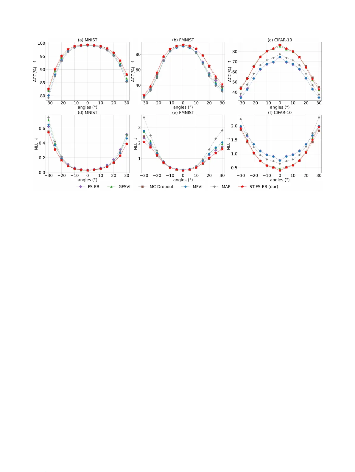
Function-Space Empirical Bayes Regularisation with Student’ s t Priors Pengcheng Hao 1 Ercan Engin Kuruoglu 1 1 Institute of Data and Information, Tsinghua Shenzhen International Graduate School, Shenzhen, China Abstract Bayesian deep learning (BDL) has emerged as a principled approach to produce reliable uncer- tainty estimates by integrating deep neural net- works with Bayesian inference, and the selection of informativ e prior distributions remains a signifi- cant challenge. V arious function-space variational inference (FSVI) re gularisation methods hav e been presented, assigning meaningful priors ov er model predictions. Howe ver , these methods typically rely on a Gaussian prior , which fails to capture the heavy-tailed statistical characteristics inherent in neural network outputs. By contrast, this work pro- poses a novel function-space empirical Bayes regu- larisation framew ork—termed ST -FS-EB—which employs heavy-tailed Student’ s t priors in both parameter and function spaces. Also, we approxi- mate the posterior distribution through v ariational inference (VI), inducing an e vidence lower bound (ELBO) objecti ve based on Monte Carlo (MC) dropout. Furthermore, the proposed method is ev al- uated against v arious VI-based BDL baselines, and the results demonstrate its robust performance in in- distribution prediction, out-of-distrib ution (OOD) detection and handling distribution shifts. 1 INTR ODUCTION The remarkable predictive accuracy of deep neural netw orks (DNNs) has established them as the cornerstone of mod- ern artificial intelligence. Y et, a closer examination re veals a fundamental blind spot: a DNN, no matter how accu- rately it predicts, remains oblivious to what it does not know Gawliko wski et al. [2023]. This distinction between "knowing" and "knowing that one knows" lies at the heart of intelligent decision-making. In high-stakes en vironments, a model’ s silence about its o wn uncertainty—e.g., failing to flag misdiagnosis risks in medical imaging Lambert et al. [2024] or misjudging pedestrian presence in autonomous driving W ang et al. [2025]—represents not merely a tech- nical limitation but a practical hazard. The question then is not only ho w to make predictions b ut also how to equip models with the capacity to express doubt. Bayesian neural networks (BNNs) offer a principled response to this chal- lenge Jospin et al. [2022]. By casting network weights as random variables go verned by prior distributions and pursu- ing posterior inference, BNNs move be yond point estimates to produce predictions together with uncertainty . T o infer the posterior distribution o ver weights, researchers ha ve ex- plored a v ariety of approaches, including Markov Chain Monte Carlo (MCMC), Laplace approximation, and v aria- tional inference (VI). Most BNNs employ Gaussian priors, yet both network parameters and predictiv e distributions often e xhibit hea vy-tailed beha viour in practice Fortuin et al. [2022]. T o accommodate this heavy-tailed beha viour, recent works ha ve adopted hea vy-tailed distributions as priors for the model weights Fortuin et al. [2021], Xiao et al. [2023], Harrison et al. [2025]. Ho we ver , these weight-space meth- ods struggle to incorporate meaningful prior knowledge into BNNs, as the relationship between weights and predictions is highly intricate. An alternativ e paradigm shifts inference from weight space to function space. Instead of placing priors on model param- eters, functional VI (FVI) Sun et al. [2019] defines inter - pretable prior distributions directly o ver model predictions and optimises a functional e vidence lo wer bound (ELBO). Howe ver , this conceptual shift comes at a cost: the Kull- back–Leibler (KL) di ver gence between infinite-dimensional stochastic processes lacks a closed-form expression. Sun et al. [2019] approximates the KL div ergence with the spec- tral Stein gradient estimator (SSGE) Shi et al. [2018], in- troducing significant computational ov erhead and limiting the scalability of the FVI in real-world settings. By contrast, linearisation-based function-space VI (FSVI) Rudner et al. [2022] methods impose Gaussian priors on model parame- ters and approximate the induced functional distrib ution as a Gaussian process (GP). This yields a tractable, closed-form approximation of the KL div ergence between prior and pos- terior Immer et al. [2021], Rudner et al. [2022], Cinquin and Bamler [2024]. Ho wev er , the linearisation strategy , though con venient, distorts the true function mapping and imposes a heavy computational burden due to the need to evaluate Jacobian matrices. By contrast, the function-space empir- ical Bayes (FS-EB) approach Rudner et al. [2023, 2024a] introduces regularisation simultaneously in both parameter and function spaces, circumventing the need for linearisa- tion. Ho wev er , all these functional methods are b uilt upon Gaussian assumptions, limiting their ability to adequately model heavy-tailed beha viour . In comparison, this work considers a ne w FS-EB frame- work based on Student’ s t priors (ST -FS-EB). The benefits are twofold: 1) the hea vy-tailed nature of the Student’ s t distribution provides enhanced rob ustness to outliers and model misspecification compared to the Gaussian distrib u- tion; 2) the additional degree-of-freedom (dof) parameter offers greater fle xibility in capturing the tail decay of the true underlying distribution. The main contrib utions of this work are sho wn below: 1. W e present a Student’ s t prior-based FS-EB frame work, which employs an empirical functional prior deriv ed from Student’ s t -distributed weights and a functional likelihood defined by a Student’ s t process. 2. W e adopt Monte Carlo (MC) dropout as the v ariational distribution to approximate the posterior within a VI framew ork, deriving an MC dropout-based ELBO ob- jectiv e. 3. Our method is compared against a range of function- space and parameter-space re gularisation baselines on fiv e real-world benchmarks. The results demonstrate that ST -FS-EB achie ves robust performance under both standard and distribution-shift settings. The remainder of this paper is organised as follows. Sec- tion 2 re views the related work, while Section 3 presents the theoretical background. Section 4 then introduces the proposed ST -FS-EB method. The experimental e valuation is reported in Section 5, and Section 6 concludes the paper . 2 RELA TED WORK 2.1 WEIGHT -SP A CE V ARIA TIONAL INFERENCE REGULARISA TION Hinton and V an Camp [1993] pioneers the first v ariational Bayesian approach for neural networks, using a diagonal Gaussian approximation of the weight posterior to imple- ment minimum description length (MDL) regularisation. Also, Grav es [2011] extends the variational method to com- plex neural network architectures by estimating the gra- dients of model parameters via MC sampling. Howe ver , both methods require substantial computational costs, mak- ing them impractical for large-scale neural networks. By contrast, Kingma and W elling [2014] introduces a repa- rameterization trick, which enables straightforward optimi- sation of the variational ELBO using standard stochastic gradient methods. Then Blundell et al. [2015] introduces a Bayes by Backprop method, a VI algorithm compatible with backpropagation that learns distributions o ver model weights by minimising the ELBO. Building upon this line of research, Gal and Ghahramani [2016] proposes the MC dropout method, establishing a theoretical connection be- tween dropout training and approximate Bayesian inference. 2.2 FUNCTION-SP A CE V ARIA TIONAL INFERENCE REGULARISA TION Initial FSVI studies focus on directly approximating pos- terior distributions ov er functions induced by neural net- works. In particular , W ang et al. [2019] proposes a function- space particle optimisation frame work, performing VI ov er regression functions. Also, Flam-Shepherd et al. [2017] presents a function-space prior alignment approach that maps GP priors to BNN priors, allowing BNNs to inherit structured functional properties from GPs. Additionally , Sun et al. [2019] demonstrates that the KL di vergence between infinite-dimensional prior and variational functional pro- cesses can be expressed as the supremum of marginal KL div ergences o ver all finite input sets, which allows the func- tional ELBO to be approximated using finite measurement sets. Howe ver , the employed SSGE method requires high computational cost, and the function-space variational ob- jecti ve is generally ill-defined Burt et al. [2021]. By contrast, an ef ficient VI frame work for posterior approximation is enabled by Ma et al. [2019] through the use of functional im- plicit stochastic process priors to handle intractable function- space objecti ves. Also, a well-defined v ariational objectiv e is achie ved in Ma and Hernández-Lobato [2021] through a grid-functional KL div ergence built on stochastic process generators. In comparison, Khan et al. [2019], Immer et al. [2021] formulate a VI objectiv e by modelling DNNs as GPs using Laplace and GGN approximations. T o enable vari- ance parameter optimisation, Rudner et al. [2022] further introduces a fully BNN-based FSVI framework, in which the KL div ergence is rendered finite by defining the prior as the pushforward of a Gaussian distribution in weight space. Moreov er , Cinquin and Bamler [2024] proposes an inter- pretable prior construction based on a pretrained GP prior and introduces a regularised KL di vergence to ensure a well- defined v ariational objecti ve. Ho wev er , these approaches approximate the model output distrib ution through lineari- sation, which requires computationally expensi ve Jacobian ev aluations and simultaneously introduces additional ap- proximation error . In comparison, the FS-EB approach Rud- ner et al. [2023, 2024b,c] av oids linearisation and constructs an empirical functional prior by combining a weight-space prior with a GP-based functional likelihood. 3 PRELIMINAR Y This section presents the fundamental concepts that form the foundation of our proposed ST -FS-EB frame work. Specif- ically , Section 3.1 and Section 3.2 introduce the Student’ s t distribution and the Student’ s t process, respectiv ely . Fur- thermore, Section 3.3 describes the FS-EB framew ork, which serves as the basis for our method. 3.1 THE STUDENT’S T DISTRIBUTION The Student’ s t distribution Ahsanullah et al. [2014] is a continuous probability distribution, which can be viewed as a heavy-tailed generalisation of the Gaussian distrib ution and provides increased rob ustness to outliers. A univ ariate Student’ s t random variable x ∈ R with location parameter µ ∈ R , scale parameter σ > 0 and dof ν > 0 is denoted by x ∼ S T ( ν , µ, σ 2 ) . Its probability density function (PDF) is giv en by p ( x ) = Γ  ν +1 2  Γ  ν 2  √ π ν σ 2  1 + ( x − µ ) 2 ν σ 2  − ν +1 2 , (1) where Γ( · ) denotes the Gamma function. Compared with the Gaussian distribution, the polynomial decay of the tails in (1) assigns significantly higher probability mass to e x- treme ev ents. Smaller values of ν correspond to hea vier tails, implying higher robustness to outliers. Also, the Student’ s t distribution includes the Gaussian distrib ution as a limiting special case. Specifically , as the dof parameter ν → ∞ , the Student’ s t distrib ution con ver ges to a normal distribution: S T ( ν , µ, σ 2 ) − − − − → ν →∞ N ( µ, σ 2 ) . This property establishes a smooth continuum between heavy-tailed and Gaussian modelling, allo wing the Student’ s t distribution to adapti vely interpolate depending on the dof value ν . Besides, assume a random v ector x ∈ R d follows a multiv ariate Student’ s t distribution Shah et al. [2014], i.e. x ∼ MV T ( ν, µ , K ) , with the dof value ν > 2 , mean µ ∈ R d , covariance matrix K ∈ R d × d , its density can be written as p ( x ) = Γ  ν + d 2  Γ  ν 2  (( ν − 2) π ) d/ 2 | K | − 1 / 2 ×  1 + ( x − µ ) ⊤ K − 1 ( x − µ ) ν − 2  − ν + d 2 . 3.2 THE STUDENT’S T PROCESS The Student’ s t process (TP) Shah et al. [2014], Solin and Särkkä [2015] is a heavy-tailed, nonparametric distrib ution ov er functions and can be viewed as a robust generalisation of the GP Seeger [2004]. A stochastic process g defined on an input space X is called a Student’ s t process with dof ν > 2 , mean function Φ : X → R , and kernel function k : X × X → R , denoted by g ∼ T P ( ν, Φ , k ) , if for any finite set of inputs x = { x 1 , . . . , x η } , ( g ( x 1 ) , . . . , g ( x η )) ⊤ ∼ MV T ( ν, µ , K ) , (2) where µ α = Φ( x α ) , K αβ = k ( x α , x β ) and α, β = 1 , . . . , η . Also, MV T ( ν, µ , K ) can be written in a Gaus- sian scale mixture (GSM) form Solin and Särkkä [2015]. Let γ − 1 ∼ Γ( ν / 2 , ( ν − 2) / 2) denote a latent in verse-Gamma scale variable and g ( x ) | γ ∼ N ( ϕ, γ K ) , (3) then marginalising ov er γ yields the Student’ s t process in Eq. (2) . As the dof parameter ν → ∞ , the Student’ s t process con ver ges to a GP: T P ( ν, Φ , k ) − − − − → ν →∞ G P (Φ , k ) . Due to its heavy-tailed marginals, the Student’ s t process assigns higher probability to extreme function values than a GP , leading to improv ed robustness against outliers. 3.3 FUNCTION-SP A CE EMPIRICAL BA YES REGULARISA TION This section describes the FS-EB framework Rudner et al. [2023, 2024a], which combines parameter-space and function-space regularisation. The FS-EB method considers a supervised learning setting defined by a dataset D = n x ( n D ) D , y ( n D ) D o N D n D =1 = ( x D , y D ) . where the N D samples are independently and identically distributed. The inputs satisfy x ( n D ) D ∈ X ⊆ R D , and the corresponding outputs lie in a target space y ( n D ) D ∈ Y . For regression tasks, the target space is continuous with Y ⊆ R L , whereas for L -class classification problems, the targets are represented as L -dimensional binary vectors, i.e., Y ⊆ { 0 , 1 } L . The FS-EB defines an auxiliary posterior as an empirical prior , i.e., p ( θ | y c , x c ) ∝ p ( y c | x c , θ ) p ( θ ) . (4) where ( x c , y c ) = n x ( n c ) c , y ( n c ) c o N c n c =1 denotes a set of con- text points and p ( θ ) represents the prior distrib ution o ver the parameters. Moreov er , to formulate the likelihood function p ( y c | x c , θ ) , FS-EB adopts a linear model z ( x c ) · = h ( x c ; ϕ 0 ) Ψ + ϵ , (5) where h ( · ; ϕ 0 ) is a feature extractor with parameter ϕ 0 , Ψ ∼ N ( 0 , τ 1 I 1 ) and ϵ ∼ N ( 0 , τ 2 I 2 ) . Also, I 1 and I 2 are identity matrices, and the positiv e scalars τ 1 , τ 2 ∈ R + gov ern the variances of the stochastic components. Gi ve context point set x c , we hav e p ( z ( x c ) | x c ) = N  z ( x c ); 0 , K ( x c , x c )  , with the cov ariance matrix K ( x c , x c ) = τ 1 h ( x c ; ϕ 0 ) h ( x c ; ϕ 0 ) ⊤ + τ 2 I 2 . (6) V iewing this distrib ution as a likelihood over neural network outputs, FS-EB obtains the following formulation: p ( y l c | x c , θ ) = N  y l c ; [ f ( x c ; θ )] l , K ( x c , x c )  , (7) where y c = 0 and f ( · ; θ ) is the neural network parame- terised by θ . Also, [ f ( x c ; θ )] l and y l c ( l = 1 , · · · , L ) are the l -th component of f ( x c ; θ ) and y c , respectiv ely . Then the auxiliary posterior can be expressed as p ( θ | y c , x c ) ∝ p ( θ ) L Y l =1 p ( y l c | x c , θ ) . (8) Le veraging this auxiliary posterior as an empirica l prior , the posterior ov er parameters giv en the full dataset is obtained via Bayes’ rule: p ( θ | y D , x D ) ∝ p ( y D | x D , θ ) p ( θ | y c , x c ) . (9) For posterior approximation, Rudner et al. [2023, 2024a] introduce techniques grounded in maximum a posteriori (MAP) estimation and VI. 4 PR OPOSED METHOD: ST -FS-EB Follo wing the introduction of the FS-EB framework, this section presents our proposed ST -FS-EB method. In partic- ular , Section 4.1 introduces the empirical Student’ s t priors ov er functions, while Section 4.2 describes the correspond- ing empirical Bayes variational inference method for poste- rior approximation. 4.1 EMPIRICAL STUDENT’S T PRIORS O VER FUNCTIONS Analogous to Eq. (4) in the FSEB framework, we introduce an auxiliary posterior conditioned on the context inputs x c , giv en by p st ( θ | y c , x c ) ∝ p st ( y c | x c , θ ) p st ( θ ) , where both the functional likelihood p st ( y c | x c , θ ) and the parameter prior p st ( θ ) are formulated under Student’ s t assumptions. Let θ i , i = 1 , . . . , I is the i -th component of θ and N θ is the number of parameters. W e define an independent and identically distributed (i.i.d.) prior ov er each model parameter as p st ( θ i ) = S T ( θ i ; ν θ , µ θ , σ 2 θ ) (10) with zero mean, i.e., µ θ = 0 . Also, following the stochas- tic modelling strate gy in (5) , we construct the functional likelihood p st ( y c | x c , θ ) by a stochastic model z st ( x c ) · = √ γ ( h ( x c ; ϕ 0 ) Ψ + ϵ ) , where h ( · ; ϕ 0 ) , Ψ and ϵ hav e the same meaning as in (5) , and γ − 1 ∼ Γ( ν θ / 2 , ( ν θ − 2) / 2) . Then we have p ( z st ( x c ) | γ ) = N ( z st ( x c ); 0 , γ K ( x c , x c )) . where K ( x c , x c ) can be calculated by (6) . According to Eq. (2) and the GSM form in Eq. (3), we obtain p st ( z st ( x c ) | x c ) = MV T  z st ( x c ); ν θ , 0 , K ( x c , x c )  . T reating p st ( y l c | x c , θ ) as the likelihood model for neural network outputs, we define p st ( y l c | x c , θ ) = MV T  y l c ; ν θ , [ f ( x c ; θ )] l , K ( x c , x c )  (11) where [ f ( x c ; θ )] l and y l c = 0 are the l -th component of f ( x c ; θ ) and y c , respectiv ely . Then we hav e the ST -FS-EB empirical prior p st ( θ | y c , x c ) ∝ I Y i =1 p st ( θ i ) L Y l =1 p st ( y l c | x c , θ ) . (12) Remark 1 In the FS-EB framework, both the par ameter prior and the functional likelihood ar e based on Gaussian assumptions. However , existing studies have shown that practical models often exhibit heavy-tailed behaviour in both parameter distrib utions and output r esponses F ortuin et al. [2022]. This empirical evidence motivates the adop- tion of our Student’ s t -based prior p st ( θ | y c , x c ) , pr o- viding a mor e r obust and e xpr essive Bayesian modelling frame work. 4.2 EMPIRICAL BA YES V ARIA TIONAL INFERENCE This section formulates posterior inference for the proposed ST -FS-EB prior . In accordance with Eq. (9) , the posterior distribution gi ven the full dataset takes the form p st ( θ | y D , x D ) ∝ p ( y D | x D , θ ) p st ( θ | y c , x c ) . Due to the intractability of the posterior distribution p st ( θ | x D , y D ) , we adopt VI to approximate the posterior . Specif- ically , we seek to minimise the KL div ergence between a tractable variational distrib ution q ( θ ) and the posterior , i.e., min q ( θ ) ∈Q D KL  q ( θ ) ∥ p st ( θ | x D , y D )  , where Q denotes a chosen family of tractable v ariational distributions. This variational optimisation problem is equi v- alently formulated as the maximisation of the ELBO: L ( θ ) = E q ( θ )  log p ( y D | x D , θ )  − D KL  q ( θ ) ∥ p st ( θ | y c , x c )  (13) where the first term corresponds to the expected data log- likelihood under the variational posterior , encouraging ac- curate data fitting. Besides, the second term acts as a regu- larisation term that constrains q ( θ ) to remain close to the proposed ST -FS-EB empirical prior p st ( θ | y c , x c ) . V ariational approximation via MC dr opout. W e em- ploy MC dropout Gal and Ghahramani [2016] to construct a tractable variational posterior q ( θ ) . Each stochastic for - ward pass under a randomly sampled dropout mask yields a realisation θ ( s ) ∼ q ( θ ) , with θ ( s ) denoting the effecti ve pa- rameters associated with the s -th dropout mask. According to (12) and (13), the objectiv e can be approximated as ˆ L ( θ ) ≈ 1 S S X s =1 " log p ( y D | x D , θ ( s ) ) + L X l =1 log p st ( y l c | x c , θ ( s ) ) # + ρ I X i =1 log p st ( θ i ) where S denotes the number of MC samples and ρ is the MC dropout rate. Then, according to (1) , (10) , (11) , we ha ve ˆ L ( θ ) ∝ 1 S S X s =1 " log p ( y D | x D , θ ( s ) ) − ν θ + N c 2 L X l =1 log 1 + c ([ f ( x c ; θ ( s ) )] l , K ( x c , x c )) ν θ − 2 ! # − ρ ( ν θ + 1) 2 I X i =1 log  1 + θ 2 i ν θ σ 2 θ  where c ( x , Σ) · = x ⊤ Σ − 1 x is the squared Mahalanobis distance between x and the origin under cov ariance ma- trix Σ . The detailed proof is provided in Section A. For each epoch of optimisation, the training data ( x D , y D ) is randomly split into a partition of M equally-sized mini- batch  x ( m ) B , y ( m ) B  ∼ ( x D , y D ) , where m = 1 , . . . , M . Let ( x ( m ) c , y ( m ) c ) ∼ ( x c , y c ) denote the corresponding ran- domly sampled context points, we ha ve the loss function at the m -th minibatch: ˆ L ( m ) ( θ ) ∝ 1 S S X s =1 " log p ( y ( m ) B | x ( m ) B , θ ( s ) ) − ν θ + N m c 2 L X l =1 log 1 + c ([ f ( x ( m ) c ; θ ( s ) )] l , K ( m ) c ) ν θ − 2 ! # − ρ ( ν θ + 1) 2 M I X i =1 log  1 + θ 2 i ν θ σ 2 θ  (14) Algorithm 1: ST -FS-EB training process of each epoch Initialisation: training data ( x D , y D ) , model parameters θ , feature extractor h ( · ; ϕ 0 ) , MC dropout rate ρ , positiv e scalars τ 1 , τ 2 , dof parameter ν θ , scale parameter σ θ , number of MC samples S , number of batches M , number of context samples N m c , for each minibatch  x ( m ) B , y ( m ) B  ∼ ( x D , y D ) : 1. Sample context points ( x ( m ) c , y ( m ) c ) . 2. Compute loss ˆ L ( m ) ( θ ) by (14). 3. Update parameters θ . end for where N m c is the sample size in ( x ( m ) c , y ( m ) c ) and K ( m ) c = K ( x ( m ) c , x ( m ) c ) . Also, the last term is scaled by an extra factor 1 M as in Blundell et al. [2015]. Remark 2 The original FS-EB fr amework assumes Gaus- sian priors and a Gaussian variational distrib ution, yielding a closed-form expr ession for the KL diver gence between them. In contrast, our method employs heavy-tailed Stu- dent’ s t priors, which br eak this conjugacy and ther efor e pr eclude a closed-form KL diverg ence. T o accommodate this choice, we le verag e MC dr opout to implicitly construct the variational posterior , enabling scalable and tractable posterior infer ence without r equiring an explicit parametric form of q ( θ ) . Selection of Priors. T o construct the functional likelihood p st ( y c | x c , θ ) , we choose a feature extractor h ( x ; ϕ 0 ) . In our approach, this extractor is a randomly initialised neural netw ork, which naturally induces inductive biases ov er functions W ilson and Izmailo v [2020]. W e can also consider a pre-trained feature e xtractor when av ailable, as in Rudner et al. [2023, 2024a]. Selection of Context Distributions. W e select context points from an auxiliary dataset ( x c , y c ) which is semanti- cally related to b ut distrib utionally distinct from the training distribution. F or instance, when training on CIF AR-10, we sample context points from CIF AR-100 to provide rele v ant OOD contextual information. Posterior Predicti ve Distributions. At inference time, predictions are formed by averaging the outputs of multiple stochastic forward passes with dropout enabled, thereby approximating the predictiv e distribution via MC integration under the variational posterior q ( θ ) q ( y ∗ | x ∗ ) = Z p  y ∗ | f ( x ∗ ; θ )  q ( θ ) d θ ≈ 1 Ξ Ξ X ξ =1 p  y ∗ | f ( x ∗ ; θ ( ξ ) )  , T able 1: In-distribution prediction performance. Best results are in bold and second best are underlined. Metric Dataset ST -FS-EB(our) FS-EB GFSVI MC Dropout MFVI MAP A CC ↑ MNIST 99.33 ± 0.052 99.10 ± 0.067 99.17 ± 0.071 99.32 ± 0.035 99.15 ± 0.095 99.09 ± 0.062 FMNIST 92.38 ± 0.194 90.49 ± 0.218 91.97 ± 0.099 92.29 ± 0.189 90.28 ± 0.281 91.87 ± 0.242 CIF AR-10 86.52 ± 0.395 74.42 ± 0.426 84.94 ± 0.548 86.54 ± 0.364 74.85 ± 0.416 77.31 ± 23.656 PathMNIST 87.83 ± 1.143 86.80 ± 1.338 88.32 ± 1.087 87.69 ± 0.771 87.34 ± 1.253 89.15 ± 2.522 OrganAMNIST 90.16 ± 0.635 88.56 ± 0.713 87.99 ± 0.353 89.81 ± 0.560 88.55 ± 0.585 86.15 ± 1.111 ECE ↓ MNIST 0.012 ± 0.001 0.010 ± 0.002 0.003 ± 0.001 0.012 ± 0.001 0.008 ± 0.001 0.003 ± 0.001 FMNIST 0.038 ± 0.003 0.013 ± 0.003 0.012 ± 0.002 0.038 ± 0.004 0.011 ± 0.003 0.012 ± 0.003 CIF AR-10 0.021 ± 0.007 0.085 ± 0.004 0.023 ± 0.004 0.028 ± 0.005 0.083 ± 0.003 0.023 ± 0.012 PathMNIST 0.049 ± 0.009 0.024 ± 0.007 0.066 ± 0.008 0.055 ± 0.006 0.019 ± 0.003 0.068 ± 0.020 OrganAMNIST 0.026 ± 0.007 0.038 ± 0.010 0.034 ± 0.006 0.016 ± 0.002 0.046 ± 0.003 0.051 ± 0.008 NLL ↓ MNIST 0.028 ± 0.001 0.034 ± 0.001 0.026 ± 0.002 0.029 ± 0.002 0.029 ± 0.001 0.026 ± 0.001 FMNIST 0.226 ± 0.005 0.263 ± 0.005 0.225 ± 0.002 0.227 ± 0.004 0.269 ± 0.006 0.231 ± 0.005 CIF AR-10 0.398 ± 0.013 0.763 ± 0.009 0.466 ± 0.012 0.399 ± 0.010 0.752 ± 0.008 0.642 ± 0.584 PathMNIST 0.454 ± 0.069 0.405 ± 0.044 0.509 ± 0.067 0.525 ± 0.113 0.399 ± 0.038 0.512 ± 0.121 OrganAMNIST 0.317 ± 0.012 0.364 ± 0.016 0.436 ± 0.025 0.318 ± 0.016 0.360 ± 0.016 0.478 ± 0.036 T able 2: Out-of-distribution detection performance. Best results are in bold and second best are underlined. In OOD ST -FS-EB(our) FS-EB GFSVI MC Dropout MFVI MAP MNIST FMNIST 99.86 ± 0.057 100.00 ± 0.000 99.99 ± 0.003 98.59 ± 0.351 98.60 ± 0.231 98.56 ± 0.255 NotMNIST 99.96 ± 0.011 99.99 ± 0.003 99.99 ± 0.006 96.86 ± 0.286 94.06 ± 0.777 95.43 ± 0.670 MNIST -c 89.38 ± 0.569 90.90 ± 0.665 90.61 ± 0.909 84.60 ± 0.679 82.69 ± 0.943 82.30 ± 0.743 FMNIST MNIST 99.70 ± 0.170 99.63 ± 0.116 99.70 ± 0.116 81.22 ± 1.717 77.48 ± 2.726 78.40 ± 2.310 NotMNIST 96.23 ± 0.665 96.97 ± 0.289 95.30 ± 0.535 80.03 ± 1.611 70.57 ± 4.324 69.49 ± 1.552 CIF AR-10 SVHN 84.87 ± 2.269 82.53 ± 1.836 88.96 ± 1.524 85.32 ± 1.174 82.56 ± 2.690 82.70 ± 11.716 CIF AR-10C0 55.34 ± 0.429 55.08 ± 0.419 55.04 ± 0.436 55.40 ± 0.428 55.07 ± 0.382 54.73 ± 1.724 CIF AR-10C2 64.19 ± 0.784 61.71 ± 0.870 63.72 ± 0.942 64.49 ± 0.842 61.69 ± 0.794 62.52 ± 4.470 CIF AR-10C4 71.35 ± 1.225 66.27 ± 1.423 71.53 ± 1.362 71.77 ± 1.107 66.39 ± 1.381 68.97 ± 6.767 PathMNIST BloodMNIST 97.29 ± 0.957 85.85 ± 10.503 96.28 ± 3.110 71.24 ± 13.143 78.38 ± 7.713 81.05 ± 7.870 OrganAMNIST OrganSMNIST 87.85 ± 2.960 86.13 ± 1.015 88.45 ± 1.601 79.80 ± 0.608 77.73 ± 0.564 74.85 ± 1.058 where θ ( ξ ) ∼ q ( θ ) , Ξ denotes the number of MC samples used to estimate the predictiv e distribution. x ∗ and y ∗ de- note a test input and its corresponding predicted output, respectiv ely . 5 EXPERIMENTS This section presents a comprehensive e valuation of ST -FS- EB, beginning with e xperimental descriptions—including baselines, setup and implementation details—followed by three sets of experiments: (1) in-distrib ution prediction and OOD detection (Section 5.1); (2) rob ustness under distri- bution shift (Section 5.2); (3) an ablation study on the dof values of the Student’ s t prior (Section 5.3). Baselines. W e benchmark our method against a div erse set of baselines spanning both function-space and parameter- space regularisation paradigms. Specifically , we include two recent FSVI approaches: FS-EB Rudner et al. [2023] and generalised FSVI (GFSVI) Cinquin and Bamler [2024]. On the parameter-space side, we consider MC Dropout Gal and Ghahramani [2016] and mean-field VI (MFVI) Blun- dell et al. [2015], along with parameter-space MAP estima- tion Bishop and Nasrabadi [2006] as a standard baseline. Setup. W e e valuate our method on five in-distribution datasets: MNIST , FashionMNIST (FMNIST), CIF AR-10, PathMNIST , and OrganAMNIST . For OOD detection ev al- uation, we use (1)FMNIST , NotMNIST and corrupted MNIST (MNIST -C) for MNIST ; (2) MNIST and NotMNIST for FMNIST ; (3)SVHN and corrupted CIF AR-10 with sev er- ity le vels 0, 2, and 4 (denoted CIF AR-10C0, CIF AR-10C2, CIF AR-10C4) for CIF AR-10; (4) BloodMNIST for PathM- NIST ; (5) OrganSMNIST for Or ganAMNIST . For MNIST - C and CIF AR-10C0/C2/C4, multiple corruption types are considered, and we report the a verage OOD detection scores across all corruption types as the final ev aluation scores. For MNIST , FMNIST and OrganAMNIST , we employ a con- volutional neural network consisting of two con volutional layers with 32 and 64 filters of size 3 × 3 , ending with a 128- unit fully connected layer . For CIF AR-10 and PathMNIST , we use a deeper architecture comprising six con volutional layers with 32, 32, 64, 64, 128, and 128 filters (all with 3 × 3 Figure 1: Performance under distribution shift induced by image rotations. The top row ((a)–(c)) reports A CC scores, while the bottom row ((d)–(f)) shows NLL. The horizontal axes denote the rotation angle, ranging from − 30 ◦ to 30 ◦ , and the vertical axis sho ws the corresponding performance scores. kernels), capped by a dense layer with 128 hidden units. All models are trained using the Adam optimiser , and all images are normalised to the range [0 , 1] . For additional details on neural network architectures, hyperparameters and other set- tings, see Section B. In-distribution prediction performance is e valuated using classification accurac y (A CC), negativ e log-likelihood (NLL), and expected calibration error (ECE). For OOD detection, we use the area under the receiv er op- erating characteristic curve (A UR OC), with the maximum softmax probability (MSP) employed as the detection score. Implementation. All experiments are conducted with 10 MC runs, and we report both the mean and standard devi- ation. For context construction, we use related auxiliary datasets: Kuzushiji-MNIST (KMNIST) for MNIST and FashionMNIST , CIF AR-100 for CIF AR-10, DermaMNIST for PathMNIST and OrganCMNIST for OrganAMNIST . Also, the feature extractor h ( · ; ϕ 0 ) shares the same archi- tecture as the trained neural network, except that the final layer is removed. Moreo ver , we set S = 10 for training and Ξ = 10 for inference. 5.1 PREDICTION AND OOD DETECTION PERFORMANCE The in-distribution prediction and OOD detection results of our proposed ST -FS-EB, in comparison with all baseline methods, are shown in T able 1 and T able 2, respecti vely . As shown in T able 1, ST -FS-EB achiev es the highest A CC on MNIST , FMNIST , and OrganAMNIST , and remains com- petiti ve with the top-performing methods on CIF AR-10 and PathMNIST . In terms of ECE, ST -FS-EB performs com- petitiv ely on CIF AR-10 and OrganAMNIST , but exhibits higher ECE values than some baselines (e.g., GFSVI and MFVI) on MNIST , FMNIST , and PathMNIST , suggesting its v ariability in calibration performance across datasets. W ith respect to NLL, ST -FS-EB consistently achie ves the lowest values on FMNIST , CIF AR-10 and OrganAMNIST , while remaining comparable to that of the best-performing baselines. By contrast, T able 2 sho ws that ST -FS-EB consis- tently achiev es the first- or second-best performance across most OOD benchmarks and remains close to the optimal results in the other cases. Overall, ST -FS-EB achie ves a strong balance between pre- dictiv e accuracy and uncertainty estimation, with robust performance across datasets and metrics. It outperforms FS- EB and GFSVI in in-distrib ution accuracy while retaining competitiv e OOD detection. Also, the ST -FS-EB consis- tently surpasses MC Dropout, MFVI, and MAP on both prediction and OOD benchmarks in most cases. 5.2 PERFORMANCE ON DISTRIBUTION SHIFTS T o inv estigate the robustness of the proposed method un- der distribution shift, this e xperiment introduces controlled T able 3: Influence of dof values of Student’ s t priors. Best results are in bold and second best are underlined. IN Metric/OOD 2.1 3.0 5.0 10.0 20.0 Gaussian MNIST A CC 99.31 ± 0.031 99.31 ± 0.072 99.33 ± 0.052 99.34 ± 0.052 99.34 ± 0.058 99.31 ± 0.044 NLL 0.031 ± 0.001 0.030 ± 0.002 0.028 ± 0.001 0.028 ± 0.002 0.027 ± 0.001 0.031 ± 0.001 FMNIST 99.91 ± 0.042 99.85 ± 0.035 99.86 ± 0.057 99.84 ± 0.040 99.95 ± 0.016 99.90 ± 0.036 NotMNIST 99.96 ± 0.011 99.95 ± 0.010 99.96 ± 0.011 99.96 ± 0.011 99.99 ± 0.004 99.95 ± 0.013 MNIST -c 89.53 ± 0.560 89.26 ± 0.538 89.38 ± 0.569 89.25 ± 0.606 90.22 ± 0.577 89.51 ± 0.469 FMNIST A CC 92.38 ± 0.194 92.45 ± 0.211 92.40 ± 0.197 92.36 ± 0.198 92.35 ± 0.117 92.25 ± 0.238 NLL 0.226 ± 0.005 0.225 ± 0.006 0.223 ± 0.005 0.224 ± 0.006 0.223 ± 0.005 0.230 ± 0.006 MNIST 99.70 ± 0.170 99.83 ± 0.085 91.31 ± 1.356 90.47 ± 1.766 99.05 ± 0.271 97.11 ± 1.063 NotMNIST 96.23 ± 0.665 96.96 ± 0.724 89.32 ± 1.844 89.07 ± 1.697 95.31 ± 0.679 93.36 ± 0.630 CIF AR-10 A CC 87.17 ± 0.382 86.88 ± 0.612 86.81 ± 0.680 86.95 ± 0.412 86.52 ± 0.395 86.73 ± 0.349 NLL 0.380 ± 0.010 0.393 ± 0.015 0.393 ± 0.019 0.391 ± 0.009 0.398 ± 0.013 0.402 ± 0.010 SVHN 84.22 ± 2.104 84.40 ± 2.170 83.22 ± 3.230 84.18 ± 0.913 84.87 ± 2.269 86.51 ± 2.022 CIF AR-10C0 55.59 ± 0.539 55.30 ± 0.447 55.50 ± 0.676 55.38 ± 0.603 55.34 ± 0.429 55.58 ± 0.466 CIF AR-10C2 64.82 ± 1.007 64.34 ± 0.803 64.64 ± 1.293 64.33 ± 1.175 64.19 ± 0.784 65.02 ± 0.895 CIF AR-10C4 72.15 ± 1.471 71.87 ± 1.268 71.72 ± 1.906 71.46 ± 1.454 71.35 ± 1.225 72.55 ± 1.507 PathMNIST A CC 87.57 ± 1.326 87.78 ± 1.154 88.08 ± 1.237 88.02 ± 1.012 87.83 ± 1.143 88.01 ± 1.093 NLL 0.470 ± 0.110 0.423 ± 0.044 0.424 ± 0.050 0.458 ± 0.050 0.454 ± 0.069 0.441 ± 0.046 BloodMNIST 97.35 ± 1.720 96.97 ± 1.317 97.69 ± 0.973 97.43 ± 1.179 97.29 ± 0.957 97.14 ± 2.531 OrganAMNIST A CC 90.50 ± 0.531 90.16 ± 0.635 90.35 ± 0.273 89.65 ± 0.877 90.37 ± 0.937 90.55 ± 0.496 NLL 0.305 ± 0.016 0.317 ± 0.012 0.314 ± 0.008 0.354 ± 0.022 0.316 ± 0.028 0.297 ± 0.011 OrganSMNIST 81.90 ± 0.800 87.85 ± 2.960 89.86 ± 2.058 80.20 ± 0.948 83.16 ± 2.210 87.93 ± 1.208 rotational transformations to the test data without apply- ing such transformations during training, thereby ev aluat- ing the generalisation ability of our proposed method to unseen rotations. Figure 1 shows the A CC and NLL perfor- mance of ST -FS-EB and baseline methods under distribu- tion shift on MNIST , FMNIST , and CIF AR-10, while the results for PathMNIST and Or ganAMNIST are reported in Figure 2 (Section C.1)). The results demonstrate that the proposed method consistently achiev es higher A CC and lower NLL than competing approaches, with only marginal differences compared to MC Dropout in a fe w scenarios. This highlights the strong robustness of ST -FS-EB under distribution shifts compared with e xisting baselines, which is critical for safety-sensiti ve and real-world deployment scenarios. 5.3 INFLUENCE OF DEGREES OF FREEDOM IN THE STUDENT -T PRIOR This experiment studies the influence of the dof parame- ter of Student’ s t priors on the performance of ST -FS-EB. W e e v aluate a range of dof values [2 . 1 , 3 . 0 , 5 . 0 , 10 . 0 , 20 . 0] and additionally include a Gaussian prior . The experimental results are summarised in T able 3. The optimal dof value exhibits clear dataset dependence for both in-distribution prediction (A CC and NLL) and OOD detection performance. For in-distribution prediction e valuation, no single dof v alue consistently dominates across datasets. On MNIST and FM- NIST , higher dof (dof = 5.0–20.0) generally yield slightly better A CC and NLL performance. On CIF AR-10, dof = 2.1 achiev es the optimal results, indicating a preference for heavier -tailed priors. For PathMNIST , dof = 5.0 provides the best performance. In contrast, on OrganAMNIST , the Gaus- sian prior attains optimal predictiv e performance. A similar pattern is observ ed for OOD de tection. The best-performing dof configurations vary across benchmarks. For instance, dof = 20.0 performs the best on MNIST -based OOD tasks, while dof = 3.0 is optimal for FMNIST -based OOD detec- tion. The Gaussian prior remains competitive in CIF AR-10, while dof = 5.0 is generally fav ourable for PathMNIST and OrganAMNIST . These observations demonstrate that the proposed hea vy-tailed Student’ s t prior assumption pro vides meaningful modelling flexibility for real-world data, yield- ing gains in both predicti ve accuracy and OOD detection. 6 CONCLUSION This paper proposes ST -FS-EB, a Student’ s t -based function- space empirical Bayes regularisation frame work, which in- troduces heavy-tailed priors o ver both parameter and func- tional distributions. W e further deriv e an MC dropout-based ELBO objectiv e to enable scalable posterior inference. The proposed method is compared with se veral baseline meth- ods, and experiment results show that ST -FS-EB achiev es a superior balance between predictiv e accuracy and OOD de- tection performance. Also, the ST -FS-EB exhibits the most robust performance under distrib ution shifts. Moreover , the optimal dof values of the Student’ s t priors are dataset- dependent, and Student’ s t priors present better prediction and OOD detection performance than Gaussian priors in most cases. References Mohammad Ahsanullah, BM Golam Kibria, and Moham- mad Shakil. Normal and student’s t distrib utions and their applications , volume 4. Springer, 2014. Christopher M Bishop and Nasser M Nasrabadi. P attern r ecognition and machine learning , volume 4. Springer, 2006. Charles Blundell, Julien Cornebise, K oray Kavukcuoglu, and Daan W ierstra. W eight uncertainty in neural network. In International confer ence on machine learning , pages 1613–1622. PMLR, 2015. David R. Burt, Sebastian W . Ober , Adrià Garriga-Alonso, and Mark van der W ilk. Understanding variational infer - ence in function-space. In Thir d Symposium on Advances in Appr oximate Bayesian Infer ence , 2021. URL https: //openreview.net/forum?id=7P9y3sRa5Mk . T ristan Cinquin and Robert Bamler . Regularized KL- div ergence for well-defined function-space variational inference in bayesian neural networks. In ICML 2024 W orkshop on Structured Pr obabilistic Inference & Gener - ative Modeling , 2024. URL https://openreview. net/forum?id=vwfWsUKW7E . Daniel Flam-Shepherd, James Requeima, and Da vid Du- venaud. Mapping gaussian process priors to bayesian neural networks. In NIPS Bayesian deep learning work- shop , volume 3, 2017. V incent F ortuin, Adrià Garriga-Alonso, Mark van der W ilk, and Laurence Aitchison. Bnnpriors: A library for bayesian neural network inference with dif ferent prior distributions. Software Impacts , 9:100079, 2021. V incent Fortuin, Adrià Garriga-Alonso, Sebastian W . Ober , Florian W enzel, Gunnar Ratsch, Richard E T urner, Mark van der W ilk, and Laurence Aitchison. Bayesian neural network priors revisited. In International Confer ence on Learning Repr esentations , 2022. URL https:// openreview.net/forum?id=xkjqJYqRJy . Y arin Gal and Zoubin Ghahramani. Dropout as a bayesian approximation: Representing model uncertainty in deep learning. In international confer ence on machine learn- ing , pages 1050–1059. PMLR, 2016. Jakob Gawlikowski, Cedrique Rovile Njieutcheu T assi, Mohsin Ali, Jongseok Lee, Matthias Humt, Jianxiang Feng, Anna Kruspe, Rudolph T riebel, Peter Jung, Ribana Roscher , et al. A surv ey of uncertainty in deep neu- ral networks. Artificial intelligence r eview , 56(Suppl 1): 1513–1589, 2023. Alex Gra ves. Practical variational inference for neural net- works. Advances in neural information pr ocessing sys- tems , 24, 2011. James Harrison, John W illes, Paul Brunzema, and Jasper Snoek. Heteroscedastic variational last layers. In 7th Sym- posium on Advances in Appr oximate Bayesian Infer ence {\ textendash } W orkshop T rac k , 2025. Geoffre y E Hinton and Dre w V an Camp. Keeping the neu- ral networks simple by minimizing the description length of the weights. In Proceedings of the sixth annual con- fer ence on Computational learning theory , pages 5–13, 1993. Alexander Immer , Maciej K orzepa, and Matthias Bauer . Improving predictions of bayesian neural nets via local linearization. In International confer ence on artificial intelligence and statistics , pages 703–711. PMLR, 2021. Laurent V alentin Jospin, Hamid Laga, Farid Boussaid, Wray Buntine, and Mohammed Bennamoun. Hands-on bayesian neural networks—a tutorial for deep learning users. IEEE Computational Intellig ence Magazine , 17(2): 29–48, 2022. Mohammad Emtiyaz Khan, Alexander Immer , Ehsan Abedi, and Maciej K orzepa. Approximate inference turns deep networks into gaussian processes. Advances in neural information pr ocessing systems , 32, 2019. Diederik P Kingma and Max W elling. Auto-encoding variational bayes. In International Confer ence on Learning Repr esentations (ICLR) , 2014. URL https://openreview.net/forum?id= 33X9fd2- 9FyZd . Benjamin Lambert, Florence Forbes, Senan Doyle, Har- monie Dehaene, and Michel Dojat. T rustworthy clinical ai solutions: a unified re view of uncertainty quantifica- tion in deep learning models for medical image analysis. Artificial Intelligence in Medicine , 150:102830, 2024. Chao Ma and José Miguel Hernández-Lobato. Functional variational inference based on stochastic process genera- tors. Advances in Neur al Information Pr ocessing Systems , 34:21795–21807, 2021. Chao Ma, Y ingzhen Li, and José Miguel Hernández-Lobato. V ariational implicit processes. In International Confer- ence on Machine Learning , pages 4222–4233. PMLR, 2019. Dimitrios Milios, Raf faello Camoriano, Pietro Michiardi, Lorenzo Rosasco, and Maurizio Filippone. Dirichlet- based gaussian processes for lar ge-scale calibrated clas- sification. Advances in Neural Information Pr ocessing Systems , 31, 2018. T im G. J. Rudner, Sanyam Kapoor , Shikai Qiu, and An- drew Gordon W ilson. Function-space regularization in neural networks: A probabilistic perspectiv e. In F ifth Sym- posium on Advances in Appr oximate Bayesian Infer ence - F ast T rack , 2023. URL https://openreview. net/forum?id=T9X1kS5FIk . T im G. J. Rudner , Xiang Pan, Y ucen Lily Li, Ra vid Shwartz- Ziv , and Andre w Gordon Wilson. Fine-tuning with uncertainty-aw are priors makes vision and language foun- dation models more reliable. In ICML 2024 W orkshop on Structur ed Pr obabilistic Infer ence & Generative Mod- eling , 2024a. URL https://openreview.net/ forum?id=37fM2QEBSE . T im GJ Rudner , Zonghao Chen, Y ee Whye T eh, and Y arin Gal. T ractable function-space variational inference in bayesian neural networks. Advances in Neural Informa- tion Pr ocessing Systems , 35:22686–22698, 2022. T im GJ Rudner , Xiang Pan, Y ucen Lily Li, Ravid Shw artz- Ziv , and Andre w Gordon Wilson. Fine-tuning with uncertainty-aw are priors makes vision and language foun- dation models more reliable. In ICML 2024 W orkshop on Structur ed Pr obabilistic Infer ence {\ & } Generative Modeling , 2024b. T im GJ Rudner , Y a Shi Zhang, Andrew Gordon W ilson, and Julia Kempe. Mind the gap: Improving rob ustness to subpopulation shifts with group-aware priors. In Interna- tional Confer ence on Artificial Intelligence and Statistics , pages 127–135. PMLR, 2024c. Matthias Seeger . Gaussian processes for machine learning. International journal of neural systems , 14(02):69–106, 2004. Amar Shah, Andre w Wilson, and Zoubin Ghahramani. Student-t processes as alternativ es to gaussian processes. In Artificial intellig ence and statistics , pages 877–885. PMLR, 2014. Jiaxin Shi, Shengyang Sun, and Jun Zhu. A spectral ap- proach to gradient estimation for implicit distributions. In International Conference on Mac hine Learning , pages 4644–4653. PMLR, 2018. Arno Solin and Simo Särkkä. State space methods for ef ficient inference in student-t process re gression. In Arti- ficial Intelligence and Statistics , pages 885–893. PMLR, 2015. Shengyang Sun, Guodong Zhang, Jiaxin Shi, and Roger Grosse. FUNCTION AL V ARIA TION AL BA YESIAN NEURAL NETWORKS. In International Confer ence on Learning Repr esentations , 2019. URL https:// openreview.net/forum?id=rkxacs0qY7 . K e W ang, Chongqiang Shen, Xingcan Li, and Jianbo Lu. Un- certainty quantification for safe and reliable autonomous vehicles: A re view of methods and applications. IEEE T ransactions on Intelligent T ransportation Systems , 2025. Ziyu W ang, T ongzheng Ren, Jun Zhu, and Bo Zhang. Func- tion space particle optimization for bayesian neural net- works. In International Conference on Learning Rep- r esentations , 2019. URL https://openreview. net/forum?id=BkgtDsCcKQ . Andrew G W ilson and Pa vel Izmailov . Bayesian deep learning and a probabilistic perspective of generaliza- tion. Advances in neural information pr ocessing systems , 33:4697–4708, 2020. Xuanzhe Xiao, Zeng Li, Chuanlong Xie, and Fengwei Zhou. Heavy-tailed regularization of weight matrices in deep neural networks. In International Conference on Artificial Neural Networks , pages 236–247. Springer , 2023. Function-Space Empirical Bayes Regularisation with Student’ s t Priors (Supplementary Material) Pengcheng Hao 1 Ercan Engin Kuruoglu 1 1 Institute of Data and Information, Tsinghua Shenzhen International Graduate School, Shenzhen, China A THE EMPIRICAL B A YES V ARIA TIONAL OBJECTIVE VIA MC DR OPOUT In this section, we deriv e the proposed ST -FS-EB variational objecti ve. Starting from Eq. (13), we obtain: L ( θ ) = E q ( θ )  log p ( y D | x D , θ )  − D KL  q ( θ ) ∥ p st ( θ | y c , x c )  = E q ( θ )  log p ( y D | x D , θ )  + Z q ( θ )log p st ( θ | y c , x c ) q ( θ ) d θ Substituting the ST -FS-EB prior in Eq. (12) into the objectiv e, we obtain L ( θ ) ∝ E q ( θ )  log p ( y D | x D , θ )  + Z q ( θ )log Q I i =1 p st ( θ i ) Q L l =1 p st ( y l c | x c , θ ) q ( θ ) d θ = E q ( θ )  log p ( y D | x D , θ )  + L X l =1 E q ( θ )  log  p st ( y l c | x c , θ )  + I X i =1 E q ( θ )  log p st ( θ i )  − E q ( θ )  q ( θ )  T o enable a tractable VI formulation, we parameterise the v ariational distribution q ( θ ) using MC dropout. Under this approximation, the entropy term E q ( θ )  q ( θ )  becomes a constant Gal and Ghahramani [2016]. Let ρ denotes the dropout rate, we hav e L ( θ ) ∝ 1 S S X s =1 " log p ( y D | x D , θ ( s ) ) + L X l =1 log p st ( y l c | x c , θ ( s ) ) # + ρ I X i =1 log p st ( θ i ) where θ ( s ) ∼ q ( θ ) denotes the ef fective parameters associated with the s -th dropout mask. By Eq. (11), we ha ve log p st ( y l c | x c , θ ( s ) ) = log MV T  y l c ; ν θ , [ f ( x c ; θ )] l , K ( x c , x c )  Let y l c = 0 , then log p st ( y l c | x c , θ ( s ) ) = log MV T  y l c ; ν θ , [ f ( x c ; θ ( s ) )] l , K ( x c , x c )  = log " Γ  ν θ + N c 2  Γ  ν θ 2  (( ν θ − 2) π ) N c / 2 | K ( x c , x c ) | − 1 / 2 1 + [ f ( x c ; θ ( s ) )] ⊤ l K − 1 ( x c , x c )[ f ( x c ; θ ( s ) )] l ν θ − 2 ! − ν θ + N c 2 # = log " Γ  ν θ + N c 2  Γ  ν θ 2  (( ν θ − 2) π ) N c / 2 # − 1 2 log | K ( x c , x c ) | − ν θ + N c 2 log 1 + [ f ( x c ; θ ( s ) )] ⊤ l K − 1 ( x c , x c )[ f ( x c ; θ ( s ) )] l ν θ − 2 ! ∝ − ν θ + N c 2 log 1 + [ f ( x c ; θ ( s ) )] ⊤ l K − 1 ( x c , x c )[ f ( x c ; θ ( s ) )] l ν θ − 2 ! Also, according to (1) and (10), log p st ( θ i ) can be calculated by log p st ( θ i ) = log S T ( θ i ; ν θ , 0 , σ 2 θ ) = log " Γ  ν θ +1 2  Γ  ν θ 2  p π ν θ σ 2 θ  1 + θ 2 i ν θ σ 2 θ  − ν θ +1 2 # = log " Γ  ν θ +1 2  Γ  ν θ 2  p π ν θ σ 2 θ # − ν θ + 1 2 log  1 + θ 2 i ν θ σ 2 θ  ∝ − ν θ + 1 2 log  1 + θ 2 i ν θ σ 2 θ  Follo wing this, we hav e our ST -FS-BE VI objectiv e: L ( θ ) ∝ 1 S S X s =1 " log p ( y D | x D , θ ( s ) ) + L X l =1 log p st ( y l c | x c , θ ( s ) ) # + ρ I X i =1 log p st ( θ i ) ∝ 1 S S X s =1 " log p ( y D | x D , θ ( s ) ) − ν θ + N c 2 L X l =1 log 1 + [ f ( x c ; θ ( s ) )] ⊤ l K − 1 ( x c , x c )[ f ( x c ; θ ( s ) )] l ν θ − 2 ! # − ρ ( ν θ + 1) 2 I X i =1 log  1 + θ 2 i ν θ σ 2 θ  B ADDITIONAL EXPERIMENT AL DET AILS B.1 HYPERP ARAMETERS T able 4 outlines the search space for the key hyperparameters of our proposed ST -FS-EB method. W e perform hyperparameter optimisation using randomised search over this space, running a total of 300 trials for each experiment. The best configuration is chosen based on the lo west NLL achieved on the validation set. All experiments employ early stopping with a maximum of 100 training epochs and a patience of 10 epochs. Additionally , the models are trained across all tasks using the Adam optimiser with a learning rate of 5 × 10 − 4 , a numerical stability parameter ϵ 1 = 10 − 8 , momentum parameters ( β 1 , β 2 ) = (0 . 9 , 0 . 999) , and a batch size of 128. Context points are sampled from the context datasets, and unless otherwise specified, their number N m c is fixed at 32. During training, we use S = 10 MC samples from q ( θ ) to approximate the objective; at inference, predictions are av eraged ov er Ξ = 10 stochastic forw ard passes to estimate the predictiv e distribution. T able 4: Hyperparameter Ranges Hyperparameters Range v θ { 2 . 1 , 3 . 0 , 5 . 0 , 10 . 0 , 20 . 0 } σ θ { 10 ℓ | ℓ = − 6 , − 5 , . . . , 1 } τ 1 { 10 ℓ | ℓ = − 6 , − 5 , . . . , 2 } τ 2 { 10 ℓ | ℓ = − 6 , − 5 , . . . , 2 } T o ensure a fair and consistent comparison, all baseline methods emplo y the same optimiser and training protocol—including batch size, learning rate, early stopping criterion and so on. The FS-EB deri ves the empirical prior from a randomly initialised neural network, consistent with the findings of Wilson et al. W ilson and Izmailov [2020]. In GFSVI, we use a GP prior with a constant zero-mean function, where the covariance kernel hyperparameters are optimised via mini-batch log marginal likelihood maximisation, as in Milios et al. Milios et al. [2018]. Both FS-EB and GFSVI draw their context points from the same context datasets used by ST -FS-EB. Finally , for MC Dropout, MFVI, and MAP methods, the isotropic Gaussian weight prior parameters are chosen using a random search procedure. B.2 MNIST , FMNIST AND ORGANAMNIST For MNIST , FMNIST and OrganAMNIST datasets, we adopt a conv olutional neural network architecture consisting of two con volutional layers with 32 and 64 filters of size 3 × 3 , respectiv ely . Each con volutional layer is follo wed by a ReLU activ ation and a max-pooling operation. The feature representations are flattened and fed into a fully connected layer with 128 hidden units, before a final linear layer produces the classification outputs. For MC Dropout–based methods, dropout layers are placed after each con volutional block and the fully connected layer , and remain acti ve at inference time to f acilitate MC sampling. The dropout rate is set to 0.5 for MNIST and F ashionMNIST , and to 0.3 for OrganAMNIST . For MNIST and FashionMNIST , Kuzushiji-MNIST (KMNIST) is used as the context dataset, whereas OrganCMNIST is used as the context dataset for Or ganAMNIST . For MNIST and FMNIST , 10% of the training set is held out as a validation set, while for OrganAMNIST , its own v alidation set is used. B.3 CIF AR-10 AND P A THMNIST For both CIF AR-10 and PathMNIST datasets, we employ a conv olutional neural network comprising six conv olutional layers with 32, 32, 64, 64, 128, and 128 filters, each of size 3 × 3 . ReLU activ ation functions follow each con volutional layer , while max-pooling layers are applied after the second, fourth, and sixth con volutional layers to progressi vely reduce the spatial dimensions. The extracted feature maps are flattened and processed by a fully connected layer with 128 hidden units, after which a linear layer produces the final classification outputs. In MC Dropout–based methods, dropout is applied after each conv olutional block and the fully connected layer , remaining active at inference to enable MC sampling. The dropout rate is set to 0.1 for both CIF AR-10 and PathMNIST . CIF AR-100 is used as the context dataset for CIF AR-10, while DermaMNIST serves as the context dataset for PathMNIST . For CIF AR-10, 10% of the training set is held out as a validation set, whereas P athMNIST uses its provided v alidation split. For both datasets, data augmentation is performed by applying random horizontal flips with a 50% probability , followed by random cropping with a padding of 4 pixels on all sides. C ADDITIONAL SIMULA TION RESUL TS C.1 ADDITIONAL RESUL TS UNDER DISTRIBUTION SHIFTS Follo wing the e xperimental results presented in Section 5.2, this section reports additional ev aluations under distrib ution shift. Figure 2 presents the ACC and NLL performance of ST -FS-EB and the baseline methods on PathMNIST and OrganMNIST under the controlled rotational transformations. The results demonstrate that ST -FS-EB consistently achiev es superior classification accuracy and lower NLL compared to most competing methods. Although its NLL is higher than that of MFVI and MAP on PathMNIST , ST -FS-EB outperforms the other functional regularisation-based approaches. C.2 INFLUENCE OF THE NUMBER OF CONTEXT POINTS This experiment in vestigates the impact of the number of context points on model performance. W e adopt the same experimental setup as in Section 5.1, and T able 5 reports the results across multiple datasets and ev aluation metrics. The results indicate that the model is insensiti ve to the choice of context numbers { 32 , 64 , 128 } , with only marginal v ariations observed in A CC, NLL and OOD detection performance. This indicates that the proposed method does not depend critically on a specific number of context points and remains rob ust across different conte xt sizes. C.3 INFLUENCE OF TRAINING CONTEXT DISTRIB UTIONS This experiment in vestigates the impact of the context distributions on model performance. W e adopt the same experimental setup as in Section 5.1 and consider two types of context points: (i) samples drawn from the training batches (TRAIN), and (ii) samples drawn from auxiliary context datasets x c , as defined in Section 5 and Section B. T able 6 reports the results across multiple datasets and e v aluation metrics. When context points are sampled from the training dataset (TRAIN), the model consistently achie ves higher A CC scores. In contrast, using auxiliary datasets leads to a slight degradation in A CC. Howe ver , this reduction is accompanied by impro ved uncertainty qualification, reflected by lower ECE and NLL, as well as substantially better OOD detection performance. These results indicate that auxiliary context datasets enable a more fa vourable trade-of f between predictiv e accuracy and uncertainty quantification. Figure 2: Performance under distribution shift induced by image rotations. The top row ((a) (b)) reports A CC scores, while the bottom row ((c) (d)) shows NLL. The horizontal axes denote the rotation angle, ranging from − 30 ◦ to 30 ◦ , and the vertical axis sho ws the corresponding performance scores. C.4 TRAINING EFFICIENCY This experiment in vestigates the training efficiency of the proposed method. W e adopt the same experimental setup as in Section 5.1. T able 7 sho ws the a verage per-epoch training time and memory consumption of ST -FS-EB in comparison with various baselines across multiple datasets. ST -FS-EB incurs a higher computational cost than traditional weight-space regularisation methods, such as MFVI and MAP , reflecting the additional ov erhead introduced by functional regularisation. Howe ver , compared to other function-space approaches (FS-EB and GFSVI), ST -FS-EB is substantially more efficient, requiring less training time and lower memory usage across all benchmarks. This efficienc y advantage arises from two factors: 1) ST -FS-EB av oids linearisation-based approximations, thereby eliminating the computational burden of Jacobian ev aluations; 2) the use of MC dropout induces sparsity in the network structure, which reduces both computational and memory costs during training. T able 5: Influence of the number of context points. Best results are in bold. OOD detection ev aluation: for MNIST , OOD1 = FashionMNIST and OOD2 = NotMNIST ; for FashionMNIST , OOD1 = MNIST and OOD2 = NotMNIST ; for CIF AR-10, OOD1 = SVHN and OOD2 = CIF AR-10C0; for PathMNIST , OOD1=BloodMNIST ; for OrganAMNIST , OOD1=OrganSMNIST . Metric Context number MNIST FMNIST CIF AR-10 PathMNIST Or ganAMNIST A CC 32 99.33 ± 0.052 92.38 ± 0.194 86.52 ± 0.395 87.83 ± 1.143 90.16 ± 0.635 64 99.31 ± 0.035 92.42 ± 0.268 86.57 ± 0.429 87.02 ± 1.346 90.60 ± 0.457 128 99.33 ± 0.047 92.35 ± 0.218 86.66 ± 0.245 87.78 ± 1.353 90.65 ± 0.386 NLL 32 0.028 ± 0.001 0.226 ± 0.005 0.398 ± 0.013 0.454 ± 0.069 0.317 ± 0.012 64 0.029 ± 0.002 0.229 ± 0.007 0.398 ± 0.012 0.448 ± 0.066 0.297 ± 0.017 128 0.030 ± 0.002 0.230 ± 0.006 0.399 ± 0.007 0.437 ± 0.052 0.291 ± 0.013 OOD1 32 99.86 ± 0.057 99.86 ± 0.057 84.87 ± 2.269 97.29 ± 0.957 87.85 ± 2.960 64 99.92 ± 0.022 99.85 ± 0.066 86.41 ± 2.526 96.79 ± 1.176 83.15 ± 1.200 128 99.98 ± 0.005 99.69 ± 0.141 86.60 ± 1.963 97.25 ± 1.896 84.50 ± 1.004 OOD2 32 99.96 ± 0.011 96.23 ± 0.665 71.35 ± 1.225 – – 64 99.97 ± 0.013 97.17 ± 0.616 72.01 ± 1.533 – – 128 99.99 ± 0.003 96.45 ± 0.676 72.64 ± 1.271 – – T able 6: Influence of the context distributions. Best results are in bold. OOD detection e valuation: for MNIST , OOD1 = Fash- ionMNIST and OOD2 = NotMNIST ; for FashionMNIST , OOD1 = MNIST and OOD2 = NotMNIST ; for CIF AR-10, OOD1 = SVHN and OOD2 = CIF AR-10C0; for PathMNIST , OOD1=BloodMNIST ; for OrganAMNIST , OOD1=Or ganSMNIST . Dataset Setting A CC ECE NLL OOD1 OOD2 MNIST TRAIN 99.37 ± 0.048 0.015 ± 0.001 0.032 ± 0.001 99.22 ± 0.156 97.99 ± 0.460 x c 99.33 ± 0.052 0.012 ± 0.001 0.028 ± 0.001 99.86 ± 0.057 99.96 ± 0.011 FMNIST TRAIN 92.43 ± 0.237 0.039 ± 0.004 0.226 ± 0.005 85.56 ± 2.097 81.62 ± 2.170 x c 92.38 ± 0.194 0.038 ± 0.003 0.226 ± 0.005 99.70 ± 0.170 96.23 ± 0.665 CIF AR-10 TRAIN 86.53 ± 0.445 0.027 ± 0.006 0.400 ± 0.013 84.97 ± 2.594 71.95 ± 1.478 x c 86.52 ± 0.395 0.021 ± 0.007 0.398 ± 0.013 84.87 ± 2.269 71.35 ± 1.225 PathMNIST TRAIN 88.18 ± 1.160 0.053 ± 0.009 0.492 ± 0.156 76.23 ± 22.597 – x c 87.83 ± 1.143 0.049 ± 0.009 0.454 ± 0.069 97.29 ± 0.957 – OrganAMNIST TRAIN 91.21 ± 0.382 0.016 ± 0.002 0.276 ± 0.008 82.13 ± 0.469 – x c 90.16 ± 0.635 0.026 ± 0.007 0.317 ± 0.012 87.85 ± 2.960 – T able 7: Training time and memory . Metric Dataset ST -FS-EB(our) FS-EB GFSVI MC Dropout MFVI MAP T ime (s/epoch) ↓ MNIST 18.52 26.96 40.44 11.24 18.13 17.86 FMNIST 18.10 26.63 40.76 11.17 17.87 17.62 CIF AR-10 43.89 58.69 93.01 32.09 44.39 18.45 PathMNIST 74.34 97.36 136.86 52.39 71.82 45.63 OrganAMNIST 20.42 25.33 35.62 16.04 22.02 15.24 Memory (MB) ↓ MNIST 536.14 808.39 1055.66 437.84 633.32 67.09 FMNIST 536.14 808.39 1055.66 437.84 633.32 67.09 CIF AR-10 1590.82 2060.54 2605.42 1275.60 1714.07 112.83 PathMNIST 1225.31 1745.45 2098.75 983.55 1479.45 93.06 OrganAMNIST 535.58 807.85 1096.22 437.28 632.76 67.09