Neural solver for Wasserstein Geodesics and optimal transport dynamics

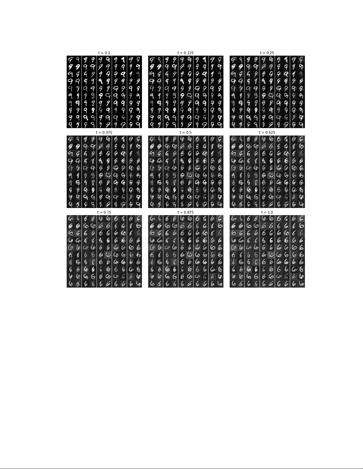
NEURAL SOL VER F OR W ASSERSTEIN GEODESICS AND OPTIMAL TRANSPOR T D YNAMICS Y AN-HAN CHEN AND HAILIANG LIU Abstract. In recent y ears, the machine learning comm unit y has increasingly embraced the optimal transp ort (OT) framework for mo deling distributional relationships. In this w ork, w e introduce a sample-based neural solver for computing the W asserstein geo desic b et w een a source and target distribution, along with the associated v elocity field. Build- ing on the dynamical formulation of the optimal transp ort (OT) problem, we recast the constrained optimization as a minimax problem, using deep neural netw orks to approx- imate the relev an t functions. This approac h not only provides the W asserstein geo desic but also recov ers the OT map, enabling direct sampling from the target distribution. By estimating the OT map, w e obtain v elo cit y estimates along particle tra jectories, which in turn allo w us to learn the full v elo cit y field. The framew ork is flexible and readily extends to general cost functions, including the commonly used quadratic cost. W e demonstrate the effectiv eness of our method through exp erimen ts on both syn thetic and real datasets. 1. Intr oduction In recent y ears, the mac hine learning comm unit y has sho wn growing interest in the optimal transp ort (OT) framew ork [54], whic h seeks to determine the most cost-effectiv e trans- formation b etw een probability distributions. Bey ond yielding an optimal transport plan, OT also induces a natural metric on the space of probability measures, the W asserstein distance, which pro vides a geometrically meaningful wa y to compare distributions. This distance has pro v en useful in a wide range of applications, including generative mo deling [4, 47, 20, 32], domain adaptation [49, 15, 14, 56], and computational geometry [46, 50]. When an optimal transp ort map exists, its computation can b e formulated as a fluid dynamics problem that minimizes kinetic energy , as introduced by Benamou and Brenier [6]. This dynamic form ulation has deep ened our understanding of W asserstein geo desics, whic h describ es the con tin uous evolution of distributions along optimal transp ort paths. The richer information pro vided b y this p ersp ectiv e not only helps the design of effi- cien t sampling metho ds from high dimensional distributions [23], but also makes learning dynamical W asserstein geo desics practically v aluable in real-world settings. In many applications – esp ecially in machine learning and data science– only empirical samples from the underlying distributions are av ailable, showing the need for sample-based metho ds (see, e.g., [20, 41, 49]). Ho w ever, accurately estimating W asserstein geo desics Date : F ebruary 26, 2026. 2020 Mathematics Subje ct Classific ation. 93E20, 49Q22. Key wor ds and phr ases. W asserstein geo desics, optimal transp ort, neural netw orks, data-driv en metho ds. Departmen t of Statistics, Iow a State Universit y , Ames, IA 50011, USA. Departmen t of Mathematics, Iow a State Universit y , Ames, IA 50011, USA. 1 2 Y AN-HAN CHEN AND HAILIANG LIU and asso ciated transp ort maps from finite samples remains a ma jor challenge, esp ecially in high-dimensional settings. Despite the recen t progress in sampled-based optimal trans- p ort methods, sev eral fundamen tal issues such as interpolation accuracy , computational efficiency , and scalability con tin ue to b e actively in v estigated. The main ob jectiv e of this article is to develop a sample-based learning framew ork using a Lagrangian descrip- tion of dynamical OT to compute the W asserstein geo desic betw een source and target distributions, along with the asso ciated v elo cit y field. Belo w w e briefly review the relev ant historical dev elopmen ts and motiv ate our prop osed w ork. 1.1. Optimal T ransp ort. The optimal transp ort (OT) problem, originally form ulated b y Monge in 1781 [45], seeks the optimal strategy to relocate the mass from a source distribution to a target distribution while minimizing the transp ortation cost. Specifically , giv en t wo nonnegative measures µ a and µ b on R d ha ving total equal mass (often assumed to b e probabilit y distributions), Monge’s problem is defined as the follo wing constrained optimization: min T Z R d c ( x, T ( x )) µ a ( dx ) , (1.1a) sub ject to T # µ a = µ b . (1.1b) Here, T : R d → R d is a measurable transp ort map, and c ( x, y ) denotes the cost of moving a unit mass from p oin t x to p oin t y , commonly taken to b e of the form c ( x, y ) = h ( x − y ) for a strongly conv ex function h . The constraint (1.1b) guarantees that the pushforw ard of µ a under T matc hes the target distribution µ b . The pushforw ard measure T # µ a is defined suc h that for an y measurable set E ∈ R d , T # µ a ( E ) = µ a ( T − 1 ( E )), or equiv alen tly , if X ∼ µ a , then T ( X ) ∼ µ b . Monge’s formulation is inherently challenging since an optimal transp ort map may not exist under general setups, esp ecially when µ a is not absolutely con tin uous with resp ect to the Leb esgue measure. F urthermore, the highly nonlinear dep endence of the transp ortation cost on the transp ort map T makes the constrained optimization problem difficult. These c hallenges led to further developmen ts. In 1942, Kantoro vic h [31] proposed a relaxed formulation where rather than seeking an explicit transp ort map T , a join t distri- bution π , called transp ort plan, on the pro duct space R d × R d is considered as a broader and more tractable framework for optimal transport. Sp ecifically , let Π( µ a , µ b ) denote the set of all join t distributions with marginals µ a and µ b , resp ectively . The Kantoro vic h form ulation of the optimal transp ort problem is then given by (1.2) inf π ∈ Π( µ a ,µ b ) Z R d × R d c ( x, y ) π ( dxdy ) . With appropriate assumptions on the cost function c ( · , · ) and the distributions µ a and µ b , Monge’s form ulation (1.1) of OT problem admits a unique optimal transp ort map T ∗ [10, 13, 54, 53]. Moreov er, the corresp onding optimal transp ort plan: π ∗ := (Id × T ∗ ) # µ a solv es the Kan toro vic h problem (1.2) [25, 53]. This connection b et w een Monge and Kan- toro vic h formulations is fundamental in optimal transp ort theory and forms the basis 3 for many mo dern computational approaches [46], while applications in high dimensional setup still remain challenging. 1.2. Densit y Control/Stochastic Control. Monge and Kantoro vic h’s formulations of the optimal transp ort problem are inheren tly static, in the sense that they fo cus on deter- mining the optimal allo cation of mass from a source distribution to a target distribution – that is, they address the question of “what go es where”, but not “how to get there”. Ho w ever, understanding the intermediate states during transp ortation is crucial for many applications in v arious domains, including reconstructing developmen tal tra jectories in cell reprogramming [48], shap e warping in computational geometry [51], and con trolling sw arm rob otics deploymen t [30, 35]. This gap can be addressed by Benamou & Brenier’s dynamic formulation [6] that captures the con tin uous evolution of mass ov er time. F or the quadratic cost function c ( x, y ) = ∥ x − y ∥ 2 , the dynamic OT problem can b e reformulated as the following v ariational problem: min v ,ρ Z S 0 Z R d L ( v ( x, t )) ρ ( x, t ) dxdt, (1.3a) sub ject to ∂ ρ ∂ t = −∇ · ( v ρ ) , (1.3b) ρ ( · , 0) = ρ a ( · ) , (1.3c) ρ ( · , S ) = ρ b ( · ) . (1.3d) Here, L ( v ) = ∥ v ∥ 2 is the Lagrangian asso ciated with kinetic energy , and ρ a , ρ b denote the densities of source and terminal distributions µ a and µ b , resp ectiv ely . The time-dep enden t v elo cit y field v = v ( x, t ) in problem (1.3) sp ecifies how to steer the mass densit y ρ ( x, t ) from ρ a to ρ b o v er the time interv al [0 , 1]. The constrain t equation (1.3b) is the contin uit y equation, which ensures mass conserv ation and is widely used in the con text of fluid dynamics. This dynamic form ulation can also b e in terpreted in a probabilistic framew ork: giv en (1.3b) and (1.3c), ρ describes the evolution of the distribution of a random pro cess X ( t ) gov erned by the ordinary differen tial equation (1.4) dX ( t ) dt = v ( X ( t ) , t ) , X (0) ∼ ρ a . In this view, the OT problem b ecomes a sp ecial case of a deterministic control problem, where the goal is to steer the distribution of the state X ( t ) from the source law ρ a to the target ρ b b y optimally c ho osing the con trol vector field v ( x, t ). Throughout the pap er, we assume without loss of generality that the terminal time is S = 1, since an y finite horizon can b e rescaled to this case. The corresp ondence b et w een OT and its dynamic form ulation extends b eyond the qua- dratic cost and holds for a broader class of cost functions. Supp ose the cost function c satisfies: c ( x (0) , x (1)) = min v ( · ,t ) Z 1 0 L  v  x ( t ) , t   dt, 4 Y AN-HAN CHEN AND HAILIANG LIU dx ( t ) dt = v ( x ( t ) , t ) for some Lagrangian L ( · ) ∈ C 1 ( R d ). A notable example is L ( v ) = ∥ v ∥ p with p ≥ 1, whic h corresp onds to the well-kno wn W asserstein- p distance [54, 53]. By (1.4) and viewing the spatial integral in (1.3a) ov er R d as an exp ectation ov er the random pro cess X ( t ), the dynamic OT problem (1.3) can b e equiv alen tly reformulated as a sto c hastic con trol problem: min v ∈V Z 1 0 E L  v  X ( t ) , t   dt, (1.5a) v ( X ( t ) , t ) = dX ( t ) dt , (1.5b) X (0) ∼ ρ a , (1.5c) X (1) ∼ ρ b . (1.5d) Here, V denotes the space of admissible control p olicies. In many data-driven scenarios, the explicit forms of ρ a and ρ b are unkno wn, and only empirical samples are av ailable. In suc h cases, a k ey ob jectiv e is to generate new samples that are consisten t with the target distribution ρ b , giv en samples from b oth ρ a and ρ b . In this w ork, w e adopt a tra jectory-based c haracterization of the OT problem and re- form ulate the sto c hastic optimal control problem (1.5) as a saddle p oint optimization. The associated functions are parameterized using neural netw orks. Once the optimiza- tion con verges, w e mo v e forward to the second phase, where the optimal v elo cit y field is reco v ered through a supervised learning problem. The main contributions of this w ork are as follo ws: • W e prop ose a learning framework to estimate the optimal map, optimal v elo c- it y field, W asserstein distance and geo desic b et ween t wo distributions giv en only through samples. W e also prov e the consistency of the corresp onding saddle p oin t form ulation. • The algorithm naturally extends to general Lagrangian functions L ( v, x, t ), includ- ing those relev ant to W asserstein- p distances. Imp ortan tly , it a voids the need to enforce the 1-Lipschitz constraint. • W e v alidate the effectiveness of the prop osed algorithm through extensiv e n umer- ical exp eriments on b oth syn thetic and real datasets, in high and low-dimensional settings, and across b oth classical and generalized Lagrangian form ulations. 1.3. Related w ork. Con v entional methods for numerically computing the W asserstein distance and geo desic t ypically rely on domain discretization, which is often mesh-dep endent [8, 24, 38]. Although effective in low-dimensional settings, these approaches b ecome com- putationally in tractable as dimensionalit y increases – so called the curse of dimensionality that frequen tly arises in real-w orld applications. A common strategy for handling high- dimensional settings is to apply entropic regularization to OT [7, 16], whic h allo ws the problem to b e efficiently solv ed using the Sinkhorn algorithm [1]. Ho w ev er, the Sinkhorn algorithm faces c hallenges when dealing with measures supp orted on contin uous domains 5 or with large n umber of samples [26] – scenarios frequently encoun tered in mac hine learn- ing applications. Neural net w orks, reno wned for their capability to appro ximate con tin uous functions [5, 17, 19], hav e b een widely used in contin uous OT algorithms to estimate transp ort maps. This approac h enables to scale OT to high-dimensional problems that are otherwise in- tractable for traditional discrete metho ds. A ma jor application of OT in this con text is generativ e mo deling – the task of learning mo dels that can generate new data samples resem bling a giv en dataset. One of the most influen tial frameworks in this area is the Generativ e Adv ersarial Netw ork (GAN) [27], whic h formulates the learning pro cess as a min-max game b etw een tw o neural netw orks: a generator and a discriminator. A notable extension is the W asserstein GAN (WGAN) [4], which incorp orates OT theory b y replac- ing the original GAN loss with the W asserstein-1 distance, resulting in improv ed training stabilit y and sample quality . How ev er, enforcing the necessary 1-Lipschitz constrain t on the discriminator has pro v en to be a significan t c hallenge [29], prompting the immedi- ate extensions and regularization strategies aimed at impro ving WGAN’s performance [29, 44, 55, 18]. Concurrently , sev eral w orks (e.g., [11, 39, 40]) ha ve sought to address the training instabilities in WGAN and to generalize the OT framework to more broader applications within generative mo deling. Bey ond GAN-based approac hes, neural net work s ha ve also b een emplo y ed to learn OT maps or transp ortation plans from finite samples. Some metho ds directly parameterize the OT map T as defined in the Monge form ulation (1.1) (e.g., [20, 56, 37]), while others mo del the sto c hastic transp ort plan π in the relaxed Kantoro vic h form ulation (1.2) (e.g. [34, 49, 42]), which is more general since a deterministic map T may not exist in all cases. When an optimal map do es exist, additional techniques suc h as regularization [33, 49], or cycle-consistency constrain ts [42] are often necessary to guide learning from transp ortation plans tow ard a w ell-defined and p ossibly unique solution. F or the special case of a quadratic cost, an optimal transp ort map T exists under the further assumption that the source distribution is absolutely con tin uous [10]. In this setting, the map can be expressed as the gradien t of a conv ex function, known as the Kantoro vic h p otential. This insigh t has motiv ated approaches that learn these p oten tials using input-con v ex neural net w orks (ICNNs) [2], leading to an active line of w ork in this direction (e.g., [43, 21, 32]). Ho w ever, most of these methods are static, fo cusing on solving single-shot OT problems b et w een t wo fixed distributions, without mo deling the in terp olation path or the dynamics of the transp ortation pro cess. In con trast, our metho d builds up on the dynamic Benamou–Brenier (BB) form ulation (1.3), which recasts OT as a fluid-flow problem and can b e naturally framed as a saddle p oin t optimization problem. The optimalit y conditions of the BB dynamic form ulation, in b oth the primal and dual spaces, are characterized by a coupled PDE system or their w eak form ulations, as explored in [41] and [28]. Instead of solving the coupled PDE system directly , [41] to ok adv antage of the strict conv exit y of the Lagrangian L ( v ) to prop ose a bidirectional learning framework, demonstrating scalability to high-dimensional settings. Meanwhile [28] in troduced GeONet, a mesh-inv arian t neural operator that learns nonlinear mapping from endp oint distributions to the en tire geo desic under the classical quadratic cost by training against the coupled PDE system. 6 Y AN-HAN CHEN AND HAILIANG LIU In contrast to these approac hes, our framew ork tackles the saddle p oin t problem directly from a sto c hastic optimization p ersp ectiv e, making it naturally compatible with general Lagrangians that may dep end on the v elo cit y field, time, and tra jectory history . 1.4. Organization. The pap er is organized as follo ws. Section 1 reviews related work in optimal transp ort and densit y con trol. In Sections 2 and 3, we presen t the form ulation of our approac h and address theoretical issues, including consistency . In Section 4, w e v ali- date our metho d through n umerical exp erimen ts on b oth synthetic and realistic datasets. Finally , Section 5 offers concluding discussions and future directions. 2. Method In this and next section, we present a data-driv en framework for learning the optimal v elo cit y field v in equation (1.5), given samples Z ∼ ρ a and Y ∼ ρ b . The approach in v olves tw o main phases. In the first phase, w e fo cus on finding the optimal transp ort map and determining the particle tra jectory X ( t ). This is formulated as a saddle-p oin t problem for the original task. W e appro ximate the transp ort map using a parameterized deep neural netw ork. Using this learned transp ort map, w e derive an estimate of the v elo cit y along the tra jectory . Ho w ever, this estimation only provides partial information, as our goal is to reco v er the full v elo cit y field. The second phase, described in Section 3, builds on this tra jectory-based velocity estimate from the first phase to learn the complete velocity field. W e b egin b y describing the first phase in detail. 2.1. T ra jectory c haracterization. T o satisfy the initial state constrain t in (1.5c), we reparameterize the tra jectory X ( t ) as X ( t ) = G ( t ; Z ) := Z + tF ( Z , t ) , 0 ≤ t ≤ 1 , where F : R d × [0 , 1] → R d is a function to b e learned. This formulation ensures that the initial condition X (0) = G (0; Z ) = Z ∼ ρ a is satisfied by construction. Here, the function G is fully and explicitly determined by F , whic h b ecomes the primary function of learning. Along the tra jectory X ( t ) = G ( t ; Z ), the corresp onding v elo cit y field is giv en b y the time deriv ative v ( X ( t ) , t ) = dG ( t ; Z ) dt . Based on this form ulation, we define the following constrained optimization problem, whic h corresp onds to problem (1.5). inf F Z 1 0 E L  dG ( t ; Z ) dt  dt, (2.1a) sub ject to G (1; Z ) ∼ ρ b , (2.1b) G ( t ; Z ) = Z + tF ( Z , t ) . (2.1c) 7 T o enforce the constrain t (2.1b), we ev aluate the discrepancy b etw een the target distri- bution ρ b and the distribution of the particles mapp ed by G (1; Z ). A common c hoice for the metric is the W asserstein-1 distance, W ( · , · ), whic h quan tities the minimal transp ort cost b et w een t w o probability measures. Notably , W ( ρ 1 , ρ 2 ) = 0 if and only if ρ 1 = ρ 2 almost ev erywhere. By replacing the terminal constrain t (2.1b) with the condition W ( ρ b , G (1; · ) # ρ a ) = 0 , where G (1; · ) # ρ a denotes the pushforward of ρ a under G (1; · ), w e obtain an equiv alen t form ulation of the optimization problem: (2.2) inf F Z 1 0 E L  dG ( t ; Z ) dt  dt, sub ject to W ( ρ b , G (1; · ) # ρ a ) = 0 , G ( t ; Z ) = Z + tF ( Z , t ) . A common strategy for solving such constrained optimization problems is to introduce a Lagrange m ultiplier λ and reformulate the problem as a saddle-p oint optimization: (2.3) sup λ inf F Z 1 0 E L  dG ( t ; Z ) dt  dt + λW ( ρ b , G (1; · ) # ρ a ) , sub ject to G ( t ; Z ) = Z + tF ( Z, t ) . R emark 2.1 . In the W asserstein geo desic formulation, F ( Z, t ) can b e c hosen to b e t - indep enden t in cases where L do es not explicitly dep end on x and is solely a con vex function of v , suc h as L ( v ) = 1 2 ∥ v ∥ 2 . This choice is exp ected to simplify b oth the algorithm and learning pro cedure. In this work, w e aim to also handle the general case with L = L ( v , x, t ), for which F = F ( Z, t ) is necessary . The general case will b e further discussed later in Section 3.2. 2.2. Kan toro vic h-Rubinstein Duality. Since w e only ha ve access to samples, directly computing the W asserstein distance W ( · , · ) in the ob jective function (2.3) is in tractable. T o ov ercome this, w e lev erage Kan toro vich-Rubinstein Dualit y [53], whic h giv es a sample- based form ulation of the W asserstein-1 distance. Let ˆ Y := G (1; Z ) denote a random sample from the pushforw ard distribution G (1; · ) # ρ a . Then,the W asserstein-1 distance W ( ρ b , G (1; · ) # ρ a ) can then b e expressed as: (2.4) W ( ρ b , G (1; · ) # ρ a ) = sup ϕ :1-Lip E h ϕ ( ˆ Y ) i − E [ ϕ ( Y )] = sup ϕ :1-Lip E [ ϕ ( G (1; Z ))] − E [ ϕ ( Y )] , where the supremum is taken ov er all 1-Lipsc hitz functions ϕ . T o further simplify the form ulation, we introduce a random v ariable U uniformly dis- tributed in [0 , 1], indep enden t of Z and Y . Incorp orating this into the saddle-point prob- lem, w e rewrite the ob jectiv e: sup λ inf F Z 1 0 E L  dG ( t ; Z ) dt  dt + λW ( ρ b , G (1; · ) # ρ a ) 8 Y AN-HAN CHEN AND HAILIANG LIU as sup λ inf F E Z ∼ ρ a ,U ∼ U (0 , 1)  L  dG ( U ; Z ) dt  + λ sup ϕ :1-Lip ( E [ ϕ ( G (1; Z ))] − E [ ϕ ( Y )]) . Assuming the order of optimization can b e exchanged, we arrive at the follo wing saddle- p oin t form ulation: inf F sup λ sup ϕ :1-Lip E  L  dG ( U ; Z ) dt  + λ ( E [ ϕ ( G (1; Z ))] − E [ ϕ ( Y )]) . (2.5) Finally , b y absorbing the scalar Lagrangian multiplier λ into the 1-Lipschitz function ϕ , w e obtain a more streamlined form ulation in which ϕ is treated as a general Lipsc hitz function. This leads to the follo wing min-max problem: inf F sup ϕ :Lip E  L  dG ( U ; Z ) dt  + ( E [ ϕ ( G (1; Z ))] − E [ ϕ ( Y )]) , (2.6a) sub ject to G ( t ; Z ) = Z + tF ( Z, t ) . (2.6b) The follo wing result guarantees the theoretical consistency of this formulation. Theorem 2.2. Supp ose the min-max pr oblem (2.6) admits a unique solution ( F ∗ , ϕ ∗ ) . Then F ∗ is also a solution to pr oblem (2.2), which is e quivalent to the original pr oblem (2.1). The proof is given in App endix A. In practical implemen tations, the exp ectations in (2.6) t ypically do not admit closed-form expressions. Nevertheless, b y the law of large n um b ers, these exp ectations can b e approx- imated to arbitrary accuracy using sample means, provided that enough indep enden t samples are av ailable. 2.3. Deep neural net w ork approximations. T o n umerically solve the optimization problem (2.6), we approximate the functions F and ϕ using deep neural net works. A fully connected feedforward neural netw ork can b e mathematically expressed as a com- p osition of linear transformations and nonlinear activ ation functions. Sp ecifically , a neural net w ork f θ : R N 1 → R N L of depth L − 2 is defined as f θ ( · ) := h L − 1 ◦ σ L − 2 ◦ h L − 2 ◦ · · · ◦ σ 1 ◦ h 1 , where eac h h j : R N j → R N j +1 , j = 1 , 2 ...., L − 1 is a linear transformation of the form h j ( x ) = W j x + b j , with weigh t matrix W j ∈ R N j +1 × N j and bias vectors b j ∈ R N j +1 . The function σ j : R → R is a nonlinear activ ation function applied comp onent-wise to the output of h j . The set of all trainable parameters in the netw ork is represented b y θ ∈ R N , whic h includes all w eigh ts and biases: W 1 , b 1 , . . . , W L − 1 , b L − 1 , with N = L − 1 X j =1 ( N j + 1) N j +1 . 9 Common activ ation functions include the h yp erb olic tangent (tanh), sigmoid, rectified linear unit (ReLU) and Leaky ReLU (LReLU) [3]. In our setting, we use tw o deep neural net w orks F θ : R d → R d and ϕ ω : R d → R , parameterized by θ and ω , resp ectiv ely , to appro ximate F and ϕ . W e select L = 5 for both F θ and ϕ ω . F or the activ ation function σ j in F θ and ϕ ω , we choose Leaky ReLU function with negativ e slop e 0 . 2 throughout the exp erimen ts in Section 4. The form ulation of this Leaky ReLU is LReLU( x ) = ( x, if x ≥ 0 0 . 2 x, otherwise. Giv en indep enden t samples { Z i } n i =1 ∼ ρ a and { Y i } n i =1 ∼ ρ b , w e discretize and appro ximate the ob jectiv e in problem (2.6) using empirical av erages. Sp ecifically , with { U j } m j =1 as inde- p enden t samples drawn from U (0 , 1), we prop ose the following finite-sample formulation (2.7) min θ max ω 1 nm m X j =1 n X i =1  L  dG θ ( U j ; Z i ) dt  + 1 n n X i =1 [ ϕ ω ( G θ (1; Z i ))] − 1 n n X i =1 [ ϕ ω ( Y i )] ! , sub ject to G θ ( t ; Z i ) = Z i + tF θ ( Z i , t ) . The proposed algorithm for solving this min-max problem is pro vided in Algorithm 1. R emark 2.3 . In fact, implemen ting the algorithm do es not require the sample sets dra wn from the t w o distributions ρ a and ρ b to ha v e the same size, nor do es it require the samples to be paired. This is because the second term in (2.7), where the terminal constraint is enforced weakly , indep enden tly appro ximates the exp ectations with resp ect to eac h distribution. This observ ation also applies to Algorithm 1 presen ted later. 2.4. Lipsc hitz constrain t on the critic neural netw ork. Our learning problem (2.7) falls within the framework of Generative Adversarial Netw orks (GANs) [27], where the actor net w ork ( F θ ) and the critic netw ork ( ϕ ω ) are adversarially trained. A k ey distinction in our setup is the application of a Lipsc hitz constrain t on the critic function in (2.6a), deriv ed from the use of the W asserstein-1 distance. Imp ortan tly , our framework enforces a general Lipsc hitz constrain t, rather than the stricter 1-Lipschitz condition commonly seen in W asserstein GANs [4]. Many subsequen t w orks [2, 32, 21, 43] ha v e addressed the challenges p osed by enforcing this non-trivial constraint. T o implemen t the Lipsc hitz condition in our parameterized critic netw ork, w e follo w the approach in [44], applying sp ectral normalization to each weigh t matrix ˜ W j of ϕ ω , and selecting 1-Lipschitz activ ation functions σ j . This ensures that the resulting netw ork is 1-Lip c hitz. W e then scale the output by a learnable parameter, inspired b y the deriv ation of our metho d b et w een (2.5) and (2.6), to generalize b ey ond the 1-Lipsc hitz case. Finally , the critic net w ork ϕ ω is defined as ϕ ω ( · ) := λ · ˜ h m − 1 ◦ σ m − 2 ◦ ˜ h m − 2 ◦ · · · ◦ σ 1 ◦ ˜ h 1 , where eac h transformed la y er ˜ h j ( x ) = ( ˜ W j x + b j ) / ∥ ˜ W j ∥ 2 , and ∥ ˜ W j ∥ 2 is the sp ectral norm of ˜ W j . Again, Leaky ReLU with negativ e slop e 0 . 2 is used as the activ ation throughout the experiments in Section 4. 10 Y AN-HAN CHEN AND HAILIANG LIU 3. Velocity field reco ver y 3.1. V elo cit y field reco v ery. Keep in mind that in problem (1.5), a key ob jective is to reco v er the full v elo cit y field v ( x, t ) – meaning we seek to determine the v alue of the v ector field at an y lo cation x ∈ R d and time t ∈ [0 , 1]. Ho w ev er, the learning framework prop osed for problem (2.6) do es not directly yield an explicit representation of v ( x, t ). T o illustrate this, let F θ ∗ denote the n umerical solution to problem (2.6). The estimated tra jectory G θ ∗ ( t ; z ) starting at z ∈ R d is giv en b y G θ ∗ ( t ; z ) := z + tF θ ∗ ( z , t ) . Using this learned tra jectory G θ ∗ and equation (1.5b), we can estimate the v elo cit y along the tra jectory as v θ ∗ ( G θ ∗ ( t ; z ) , t ) := dG θ ∗ ( t ; z ) dt . Ho w ever, this only provides the v alues of the velocity along tra jectories, not the full v elo cit y field v ( x, t ) where x and t are indep endent. T o reco v er the complete v elo cit y field v ( x, t ), where the spatial and temp oral argumen ts are indep endent, we in tro duce another neural net w ork v η to approximate the true time- v arying velocity field. W e treat v θ ∗ ( G θ ∗ ( U ; Z ) , U ) as samples from the ground truth and train v η using supervised learning. By employing the squared error loss, w e formulate the following optimization problem to learn the velocity field v for problem (1.5): (3.1) min η 1 mn m X j =1 n X i =1     v η ( G θ ∗ ( U j ; Z i ) , U j ) − dG θ ∗ ( U j ; Z i ) dt     2 . As our Phase 2, this pro cedure is describ ed in Algorithm 2. R emark 3.1 . Regarding the samples Z i and U j used for training in Phase 2, w e recommend dra wing fresh samples rather than reusing those from Phase 1. This helps prev en t Phase 2 from simply memorizing velocities along the specific tra jectories learned in Phase 1. In the syn thetic exp erimen ts presented in Section 4, where the true velocity field v ∗ is a v ailable, w e observe no significan t difference in the error b et ween v η and v ∗ when comparing fresh samples to reused Phase 1 samples. Ho w ever, this ma y b e due to the relative simplicit y of the synthetic settings, whic h mak es the velocity field easier to learn. Moreo v er, since the tra jectories learned in Phase 1 are treated as ”ground truth” during sup ervised training in Phase 2, a zero Phase 2 loss do es not guarantee conv ergence of v η to v ∗ (see App endix B for more details). In summary , the prop osed framework addresses problem (1.5) in tw o phases: first by solving (2.7) to estimate the geo desic, and then b y solving (3.1) to learn the full velocity field. It is w orth noting that in some applications, the ob jectiv e is to generate additional samples from ρ b , in terp olate in termediate tra jectories, or estimate v elo cities along the transp ort paths. In suc h cases, implementing Phase 1 to obtain the transport map is already sufficien t, and Phase 2 – aimed at recov ering the Euler v elocity field – is not necessary . 11 3.2. Extension to general Lagrangian. Our metho d extends naturally to time-dep endent optimal transp ort problems, in whic h the transp ortation cost also dep ends on the trans- p ort tra jectory , rather than just the initial and terminal p oin ts. In such settings, a t ypical Lagrangian tak es the form L ( x, v , t ) = ∥ v ∥ 2 2 − V ( x ) , where V : R d → R is a p oten tial function [53]. F or a general Lagrangian, the existence and uniqueness of an optimal solution are guaranteed when L ( x, v , t ) is strictly conv ex and sup erlinear in the v elo cit y v ariable v [12, 53, 22, 9]. F or further details ab out the time-dep enden t optimal transp ort, we refer the reader to Villani [53] and Chen et al. [12]. The Lagrangian in our previous setup (1.5) is a sp ecial case of this more general form ulation: b y selecting V ( x ) = 0, we recov er the simpler form L ( x, v , t ) = L ( v ) = ∥ v ∥ 2 2 . Using a similar approach to that in Section 2, w e can n umerically solv e the more general v ersion of the dynamical optimal transp ort problem: min v Z 1 0 E L  X ( t ) , v  X ( t ) , t  , t  dt, v ( X ( t ) , t ) = dX ( t ) dt , X (0) ∼ ρ a , X (1) ∼ ρ b . In practice, w e implement this by replacing the simple kinetic energy with the more general Lagrangian: L  G θ ( U j ; Z i ) , dG θ ( U j ; Z i ) dt , U j  for the corresp onding term in (2.7) and Algorithm 1. A n umerical experiment in this general setting will b e given in Section 4. It is worth noting that many existing metho ds based on the Benamou–Brenier dynamical form ulation (e.g., [41, 28]) primarily fo cus on the setting where L = L ( v ) dep ends solely on v and is strictly con v ex. In suc h case, the asso ciated Hamiltonian H ( p ) := sup v v · p − L ( v ) admits an explicit form. In con trast, our framew ork naturally extends to the more general class of Lagrangian considered ab o v e. 4. Numerical Experiments In this section, w e ev aluate our algorithms on b oth syn thetic and real datasets. The neural net w orks used for the transp ort map G θ , the critic ϕ ω , and the v elo cit y field v η eac h consists of three hidden la yers and are trained using RMSprop optimizer [52]. W e adopt the Leaky ReLU activ ation function with a negativ e slop e of 0 . 2 across all exp eriments. Except for the general Lagrangian case in Synthetic-4, we use the standard quadratic Lagrangian L ( v ) = ∥ v ∥ 2 . Under this choice, the first term in the ob jective function (2.7) serv es as an estimate of the squared W asserstein-2 distance b et ween the source and target distributions. F or the random v ariable { U j } m j =1 used in Algorithm 1 and 2, we adopt m = 10 equally spaced time steps from t = 0 . 1 to t = 1 . 0 in Synthetic-1 through Synthetic-3. W e 12 Y AN-HAN CHEN AND HAILIANG LIU Algorithm 1 T raining Pro cedure for Solving Problem (2.7). 1: Input: Sample size n ; num ber of time samples m ; Lagrangian L ( v ). 2: Initialize net w orks F θ and ϕ ω . Define G θ ( t ; z ) := z + tF θ ( z , t ) for ( z , t ) ∈ R d × [0 , 1]. 3: while θ has not con v erged do 4: Sample { Z i } n i =1 i . i . d ∼ ρ a and { Y i } n i =1 i . i . d ∼ ρ b . 5: Compute the ob jective function for ϕ ω ℓ ω ← 1 n n X i =1 [ ϕ ω ( G θ (1; Z i ))] − 1 n n X i =1 [ ϕ ω ( Y i )] . 6: Up date ω by ascending ℓ ω . 7: Sample { Z i } n i =1 i . i . d ∼ ρ a and { U j } m j =1 i . i . d ∼ U (0 , 1). 8: Compute the ob jective function for F θ ℓ θ ← 1 mn m X j =1 n X i =1 L  dG θ ( U j ; Z i ) dt  + 1 n n X i =1 ϕ ω ( G θ (1; Z i )) . 9: Up date θ by descending ℓ θ . 10: end while 11: Output: T rained geo desic G θ and critic ϕ ω . Algorithm 2 T raining Pro cedure for Solving Problem (3.1). 1: Input: T rained neural net w ork G θ ∗ from Algorithm 1. 2: Initialize the netw ork v η . 3: while η has not con v erged do 4: Sample { Z i } n i =1 i . i . d ∼ ρ a and { U j } m j =1 i . i . d ∼ U (0 , 1). 5: Compute the ob ject function for v η ℓ η = 1 mn m X j =1 n X i =1     v η ( G θ ∗ ( U j ; Z i ) , U j ) − dG θ ∗ ( U j ; Z i ) dt     2 2 . 6: Up date v η b y descending ℓ η . 7: end while 8: Output: T rained v elo cit y field v η . set m = 20 in Syn thetic-4 and in the Real Data case. In Synthetic-1 and Syn thetic-3 where the analytical v elo cit y field v ∗ are av ailable, w e compare v ∗ with the learned v η in the Appendix B. F or the real data scenario, w e apply our algorithm to the MNIST handwritten digits dataset [36], which serv es as a high-dimensional b enchmark. The v elo cit y fields rep orted in this section are trained with fresh samples Z i and U j . That is, new samples are drawn for the sup ervised training in Phase 2. Syn thetic Exp erimen ts 13 Figure 1. Phase 1 of Synthetic-1: Samples of the source distribution ρ a (op en circle at the b ottom left corner) are transp orted to the upp er right corner. Each gray line illustrates the learned tra jectory G θ ( t ; · ) # ρ a . The con tour sho ws the true log density of ρ b . Syn thetic-1: 2D-Gaussian. In this 2D example, b oth ρ a and ρ b are Gaussian distri- butions ρ a = N  0 0  ,  1 0 0 1  , ρ b = N  6 6  ,  1 . 5 0 . 5 0 . 5 1 . 5  . Figure 1 shows the learned tra jectories of samples of ρ a in Phase 1. Figure 2 presen ts the learned v elo cit y field at selected time p oin ts in Phase 2. Syn thetic-2: Mixture of 2D-Gaussians. Here, ρ a is a standard 2-dimensional Gauss- ian, and ρ b is a mixture of 4 Gaussian comp onen ts with the same co v ariance matrix as ρ a , p ositioned at the corners of a square. Figure 3 and 4 present the learned geo desic and v elo cit y field. Syn thetic-3: 10D-Gaussians. F or this exp erimen t in the 10-dimensional space, ρ a is chosen to b e a standard Gaussian and ρ b another Gaussian. The learned geo desic and v elo cit y field pro jected to the 2-dimensional space are shown in Figure 5 and 6, resp ectiv ely . Syn thetic-4: 2D Harmonic Oscillation with general Lagrangian. In this example, w e consider the 2-dimensional harmonic oscillation. Sp ecifically , for x = ( x 1 , x 2 ) and v in R 2 , consider the Lagrangian L ( x, v ) = 1 2  ∥ v ∥ 2 − ω 2 1 x 2 1 − ω 2 2 x 2 2  , where ω 1 , ω 2 > 0 are given. Solv e the optimization problem: min v 1 2 Z 1 0 E  ∥ v ( X ( t ) , t ) ∥ 2 − ω 2 1 X 2 1 ( t ) − ω 2 2 X 2 2 ( t )  , 14 Y AN-HAN CHEN AND HAILIANG LIU Figure 2. Phase 2 of Synthetic-1: learned v elo cit y fields at selected time p oin ts. The arro ws illustrate the direction and magnitude of the learned v elo cit y . v ( X ( t ) , t ) = dX ( t ) dt , X (0) ∼ ρ a , X (1) ∼ ρ b . W e consider the case ω 1 = 1 . 2 , ω 2 = 0 . 1 and the source and target distributions are defined as ρ a = N  m a, 1 m a, 2  ,  0 . 01 0 0 0 . 01  , ρ b = N  m b, 1 m b, 1  ,  0 . 01 0 0 0 . 01  , where m a, 1 = m a, 2 = 3 , m b, 1 = m b, 2 = 5. In this setting, the analytical solution X ( t ) is a v ailable (4.1) X 1 ( t ; x ) = sin ( ω 1 (1 − t )) + sin ( ω 1 t ) sin ω 1 x 1 + sin ( ω 1 t ) sin ω 1 ( m b, 1 − m a, 1 ) X 2 ( t ; x ) = sin ( ω 2 (1 − t )) + sin ( ω 2 t ) sin ω 2 x 2 + sin ( ω 2 t ) sin ω 2 ( m b, 2 − m a, 2 ) 15 Figure 3. Phase 1 of Synthetic-2: Samples of the source distribution ρ a (op en circle at the cen ter) are transp orted to the four corners. Each gray line illustrates the learned tra jectory G θ ( t ; · ) # ρ a . The contour sho ws the true log density of ρ b . This analytical tra jectory and the learned geo desic in Phase 1 are shown in Figure 7. In Figure 8, the velocity field learned in Phase 2 is sho wn. Real Data: MNIST digit transformation. As a high-dimensional example (28 × 28 dimensions), w e consider the MNIST dataset. Sp ecifically , we aim to learn a transp ort map from digit 6 (representing ρ a ) to digit 9 (represen ting ρ b ). Figure 9 and 10 illustrate the learned geo desic tra jectory in Phase 1. Commen t on the results of the n umerical exp eriments. W e observ ed that the generated samples G (1; · ) # ρ a exhibit patterns similar to the target distribution ρ b , as ev- idenced b y comparing the empirical distribution of the pushed op en circle to the true log densit y contour in synthetic cases, and b y the conv ergence of the W asserstein-1 distance to w ard zero during Phase 1 training in most cases (see App endix B for details during training). F urthermore, visualization of particle tra jectories suggest that the transp ort of samples o ccurs efficiently . How ev er, w e note that the ob jective function v alues often fluc- tuate during Phase 1 training, which may b e due to the inherent instabilit y of optimizing a min-max problem in volving t wo adv ersarial net w orks. In some cases (e.g., Figure 3 of Syn thetic-2), the mapp ed distribution do es not fully match the target distribution, as indicated b y the failure of the estimated W asserstein-1 distance to conv erge to zero. W e ac kno wledge the existence of additional regularization tec hniques for the critic function (e.g., [29]) that might improv e target distribution matc hing in Phase 1. T o address insta- bilit y , alternativ e optimization methods ma y help impro v e p erformance. In addition, w e observ e that neural netw ork h yp erparameters – suc h as the choice of activ ation function, 16 Y AN-HAN CHEN AND HAILIANG LIU Figure 4. Phase 2 of Synthetic-2: learned v elo cit y fields at selected time p oin ts. The arro ws illustrate the direction and magnitude of the learned v elo cit y . depth, width, and learning rate – can significantly affect p erformance, including the qual- it y of distribution matc hing. Th us, additional regularization and careful hyperparameter tuning are tw o pra ctical strategies for improving p erformance in cases where matc hing the target distribution and the pushfo ward distribution is particularly challenging. In Phase 2, where the complete v elo cit y field is learned, w e observe that the discrepancy b et ween the learned and the true v elo cit y fields (e.g., Figure 16 in App endix B) do es not fully v anish. This ma y stem from using the Phase 1 learned tra jectories as samples for ground truth, ev en though they are only appro ximations. 5. Conclusion In this paper, we propose a sample-based learning framew ork to estimate the OT geo desic and corresp onding v elo cit y field for transp orting the source distribution into the target distribution with minimum cost. F urthermore, the learning algorithm can be naturally applied to general Lagrangian where the transp ortation cost may dep ends on the velocity field, transp ort tra jectory and time, including the classical case of simple kinetic energy . 17 Figure 5. Phase 1 of Synthetic-3: 2-dimensional pro jection of the 10- dimensional distributions. Samples of the source distribution ρ a (op en circle at the bottom left corner) are transp orted to the upp er right corner. Each gra y line illustrates the learned tra jectory G θ ( t ; · ) # ρ a . The con tour sho ws the true log density of ρ b . W e demonstrate the p erformance of our algorithm through a series of exp eriments includ- ing syn thetic and realistic data, high-dimensional and lo w-dimensional setups, classical and general Lagrangian. Declara tions Conflict of In terest. The authors declare that they ha v e no kno wn comp eting financial in terests or p ersonal relationships that could ha v e app eared to influence the w ork rep orted in this pap er. Data Av ailabilit y. The datasets generated during the the study are av ailable from the corresponding author on reasonable request. The MNIST dataset used is a publicly a v ailable b enchm ark. References [1] Jason Altsch uler, Jonathan Niles-W eed, and Philipp e Rigollet, Ne ar-line ar time appr oximation al- gorithms for optimal tr ansp ort via sinkhorn iter ation , Adv ances in Neural Information Pro cessing Systems, v ol. 30, Curran Asso ciates, Inc., 2017. [2] Brandon Amos, Lei Xu, and J Zico Kolter, Input c onvex neur al networks , International Conference on Mac hine Learning, PMLR, 2017, pp. 146–155. [3] Andrea Apicella, F rancesco Donnarumma, F rancesco Isgr` o, and Rob erto Prevete, A survey on mo d- ern tr ainable activation functions , Neural Netw orks 138 (2021), 14–32. [4] Martin Arjovsky , Soumith Chin tala, and L ´ eon Bottou, Wasserstein gener ative adversarial networks , In ternational Conference on Machine Learning, PMLR, 2017, pp. 214–223. 18 Y AN-HAN CHEN AND HAILIANG LIU Figure 6. Phase 2 of Synthetic-3: learned v elo cit y fields at selected time p oin ts. The arro ws illustrate the direction and magnitude of the learned v elo cit y . [5] Andrew R Barron, Universal appr oximation b ounds for sup erp ositions of a sigmoidal function , IEEE T ransactions on Information theory 39 (1993), no. 3, 930–945. [6] Jean-David Benamou and Y ann Brenier, A c omputational fluid me chanics solution to the Monge- Kantor ovich mass tr ansfer pr oblem , Numerische Mathematik 84 (2000), no. 3, 375–393. [7] Jean-David Benamou, Guillaume Carlier, Marco Cuturi, Luca Nenna, and Gabriel Peyr ´ e, Iter ative Br e gman pr oje ctions for r e gularize d tr ansp ortation pr oblems , SIAM Journal on Scientific Computing 37 (2015), no. 2, A1111–A1138. [8] Jean-David Benamou, Brittan y D F ro ese, and Adam M Oberman, Two numeric al metho ds for the el- liptic Monge-Amp` er e e quation , ESAIM: Mathematical Mo delling and Numerical Analysis 44 (2010), no. 4, 737–758. [9] Patric k Bernard and Boris Buffoni, Optimal mass tr ansp ortation and mather the ory , Journal of the Europ ean Mathematical So ciet y 9 (2007), no. 1, 85–121. [10] Y ann Brenier, Polar factorization and monotone r e arr angement of ve ctor-value d functions , Comm u- nications on Pure and Applied Mathematics 44 (1991), no. 4, 375–417. [11] Jiezhang Cao, Langyuan Mo, Yifan Zhang, Kui Jia, Ch unh ua Shen, and Mingkui T an, Multi-mar ginal Wasserstein GAN , Adv ances in Neural Information Pro cessing Systems 32 (2019). 19 Figure 7. Phase 1 of Syn thetic-4: Left panel presen ts the analytical tra- jectories (4.1) of 20 samples from ρ a (op en circle at the b ottom left corner). In the right panel, those 20 samples are transp orted b y the learned map, where the gray lines illustrate the learned tra jectories G θ ( t ; · ) # ρ a . The con- tour in the right panel sho ws the true log density of ρ b . [12] Y ongxin Chen, T ryphon T Georgiou, and Michele Pa v on, Optimal tr ansp ort over a line ar dynamic al system , IEEE T ransactions on Automatic Con trol 62 (2016), no. 5, 2137–2152. [13] , Optimal tr ansp ort in systems and c ontr ol , Ann ual Review of Con trol, Rob otics, and Au- tonomous Systems 4 (2021), no. 1, 89–113. [14] Nicolas Courty , R ´ emi Flamary , Amaury Habrard, and Alain Rak otomamonjy , Joint distribution optimal tr ansp ortation for domain adaptation , Adv ances in Neural Information Pro cessing Systems 30 (2017). [15] Nicolas Court y , R ´ emi Flamary , Devis T uia, and Alain Rak otomamonjy , Optimal tr ansp ort for domain adaptation , IEEE transactions on pattern analysis and machine intelligence 39 (2016), no. 9, 1853– 1865. [16] Marco Cuturi, Sinkhorn distanc es: Lightsp e e d c omputation of optimal tr ansp ort , Adv ances in Neural Information Pro cessing Systems 26 (2013), 2292—-2300. [17] George Cyb enko, Appr oximation by sup erp ositions of a sigmoidal function , Mathematics of con trol, signals and systems 2 (1989), no. 4, 303–314. [18] Nhan Dam, Quan Hoang, T rung Le, T u Dinh Nguy en, Hung Bui, and Dinh Phung, Thr e e-player Wasserstein GAN via amortise d duality , Pro ceedings of the Twen ty-Eigh th In ternational Joint Con- ference on Artificial Intelligence, IJCAI-19, International Joint Conferences on Artificial Intelligence Organization, 7 2019, pp. 2202–2208. [19] Tim De Ryck, Sam uel Lan thaler, and Siddhartha Mishra, On the appr oximation of functions by tanh neur al networks , Neural Netw orks 143 (2021), 732–750. [20] Jiao jiao F an, Sh u Liu, Shao jun Ma, Haomin Zhou, and Y ongxin Chen, Neur al Monge map estimation and its applic ations , T ransactions on Machine Learning Research (2023). [21] Jiao jiao F an, Amirhossein T aghv aei, and Y ongxin Chen, Sc alable c omputations of Wasserstein b aryc enter via input c onvex neur al networks , In ternational Conference on Machine Learning, PMLR, 2021, pp. 1571–1581. [22] Alessio Figalli, Optimal tr ansp ortation and action-minimizing me asur es , v ol. 8, Edizioni della Nor- male, 2008. [23] Chris Finlay , J¨ orn-Henrik Jacobsen, Levon Nurb eky an, and Adam M Ob erman, How to tr ain your neur al o de: The world of jac obian and kinetic r e gularization , Pro ceedings of the 37th In ternational Conference on Mac hine Learning (ICML), 2020. [24] Wilfrid Gangbo, W uchen Li, Stanley Osher, and Michael Putha wala, Unnormalize d optimal tr ans- p ort , Journal of Computational Physics 399 (2019), 108940. 20 Y AN-HAN CHEN AND HAILIANG LIU Figure 8. Phase 2 of Synthetic-4: learned v elo cit y fields at selected time p oin ts. The arro ws illustrate the direction and magnitude of the learned v elo cit y . [25] Wilfrid Gangb o and Rob ert J McCann, The ge ometry of optimal tr ansp ortation , Acta Mathematica 177 (1996), 113–161. [26] Aude Genev a y , Marco Cuturi, Gabriel Peyr ´ e, and F rancis Bach, Sto chastic optimization for lar ge- sc ale optimal tr ansp ort , Adv ances in Neural Information Pro cessing Systems 29 (2016). [27] Ian J Go odfellow, Jean Pouget-Abadie, Mehdi Mirza, Bing Xu, Da vid W arde-F arley , Sherjil Ozair, Aaron Courville, and Y oshua Bengio, Gener ative adversarial nets , Adv ances in Neural Information Pro cessing Systems, vol. 27, Curran Asso ciates, Inc., 2014. [28] Andrew Gracyk and Xiaoh ui Chen, Ge onet: a neur al op er ator for le arning the Wasserstein ge o desic , Pro ceedings of the F ortieth Conference on Uncertain ty in Artificial Intelligence, v ol. 244, PMLR, 2024, pp. 1453–1478. [29] Ishaan Gulra jani, F aruk Ahmed, Martin Arjovsky , Vincen t Dumoulin, and Aaron C Courville, Im- pr ove d tr aining of Wasserstein GANs , Adv ances in Neural Information Pro cessing Systems, vol. 30, Curran Asso ciates, Inc., 2017. [30] Daisuke Inoue, Y uji Ito, and Hiroaki Y oshida, Optimal tr ansp ort-b ase d c over age c ontr ol for swarm r o- b ot systems: Gener alization of t he Vor onoi tessel lation-b ase d metho d , IEEE Con trol Systems Letters 5 (2020), no. 4, 1483–1488. [31] Leonid Kantoro vitch, On the tr anslo c ation of masses , Managemen t Science 5 (1958), no. 1, 1–4. 21 Figure 9. Phase 1 of Real data (MNIST): Left panel contains 100 samples from the source distribution ρ a (digit 9). Right panel consists of transported samples G θ (1; · ) # ρ a , whic h is meant to match ρ b (digit 6). [32] Alexander Korotin, V age Egiazarian, Arip Asadulaev, Alexander Safin, and Evgeny Burnaev, Wasserstein-2 gener ative networks , International Conference on Learning Representations, 2021. [33] Alexander Korotin, Lingxiao Li, Aude Genev a y , Justin M Solomon, Alexander Filipp o v, and Evgen y Burnaev, Do neur al optimal tr ansp ort solvers work? a c ontinuous Wasserstein-2 b enchmark , Ad- v ances in neural information pro cessing systems 34 (2021), 14593–14605. [34] Alexander Korotin, Daniil Selikhano vyc h, and Evgen y Burnaev, Neur al optimal tr ansp ort , The Elev enth International Conference on Learning Representations, 2023. [35] Vishaal Krishnan and Sonia Mart ´ ınez, Distribute d optimal tr ansp ort for the deployment of swarms , 2018 IEEE Conference on Decision and Con trol (CDC), IEEE, 2018, pp. 4583–4588. [36] Y ann LeCun, L ´ eon Bottou, Y oshua Bengio, and Patric k Haffner, Gr adient-b ase d le arning applie d to do cument r e c o gnition , Pro ceedings of the IEEE 86 (1998), no. 11, 2278–2324. [37] Jacob Leygonie, Jennifer She, Amjad Almahairi, Sai Ra jeswar, and Aaron Courville, A dversarial c omputation of optimal tr ansp ort maps , arXiv preprint arXiv:1906.09691 (2019). [38] W uchen Li, Ernest K Ryu, Stanley Osher, W otao Yin, and Wilfrid Gangb o, A p ar al lel metho d for e arth mover’s distanc e , Journal of Scientific Computing 75 (2018), no. 1, 182–197. [39] Huidong Liu, Xianfeng Gu, and Dimitris Samaras, Wasserstein GAN with quadr atic tr ansp ort c ost , Pro ceedings of the IEEE/CVF international conference on computer vision, 2019, pp. 4832–4841. [40] Huidong Liu, Gu Xianfeng, and Dimitris Samaras, A two-step c omputation of the exact GAN Wasser- stein distanc e , International Conference on Machine Learning, PMLR, 2018, pp. 3159–3168. [41] Shu Liu, Shao jun Ma, Y ongxin Chen, Hongyuan Zha, and Haomin Zhou, L e arning high dimensional Wasserstein ge o desics , arXiv preprin t arXiv:2102.02992 (2021). [42] Guansong Lu, Zhiming Zhou, Jian Shen, Cheng Chen, W einan Zhang, and Y ong Y u, L ar ge-sc ale optimal tr ansp ort via adversarial tr aining with cycle-c onsistency , arXiv preprin t (2020). [43] Ashok Makkuv a, Amirhossein T aghv aei, Sewoong Oh, and Jason Lee, Optimal tr ansp ort mapping via input c onvex neur al networks , In ternational Conference on Machine Learning, PMLR, 2020, pp. 6672–6681. [44] T akeru Miyato, T oshiki Kataok a, Masanori Koy ama, and Y uic hi Y oshida, Sp e ctr al normalization for gener ative adversarial networks , International Conference on Learning Representations, 2018. [45] Gaspard Monge, M´ emoir e sur la th´ eorie des d´ eblais et des r emblais , Mem. Math. Ph ys. Acad. Ro yale Sci. (1781), 666–704. 22 Y AN-HAN CHEN AND HAILIANG LIU Figure 10. Phase 1 of Real data case (MNIST): Selected time slices of the transformation pro cess from ρ a (digit 9) to G θ (1; · ) # ρ a , which is mean t to matc h ρ b (digit 6). [46] Gabriel P eyr´ e and Marco Cuturi, Computational optimal tr ansp ort: With applic ations to data sci- enc e , F oundations and T rends in Machine Learning 11 (2019), no. 5-6, 355–607. [47] Litu Rout, Alexander Korotin, and Evgeny Burnaev, Gener ative mo deling with optimal tr ansp ort maps , Pro ceedings of the International Conference on Learning Representations, 2022. [48] Geoffrey Schiebinger, Jian Shu, Marcin T abak a, Brian Cleary , Vidya Subramanian, Aryeh Solomon, Josh ua Gould, Siyan Liu, Stacie Lin, Peter Berube, Lia Lee, Jenny Chen, Justin Brum baugh, Philipp e Rigollet, Konrad Ho c hedlinger, Rudolf Jaenisch, Aviv Regev, and Eric S. Lander, Optimal- tr ansp ort analysis of single-c el l gene expr ession identifies developmental tr aje ctories in r epr o gr am- ming , Cell 176 (2019), no. 4, 928–943. [49] Vivien Seguy , Bharath Bhushan Damo daran, Remi Flamary , Nicolas Courty , An toine Rolet, and Mathieu Blondel, L ar ge-sc ale optimal tr ansp ort and mapping estimation , ICLR 2018-In ternational Conference on Learning Represen tations, 2018, pp. 1–15. [50] Justin Solomon, F ernando de Go es, Gabriel Peyr ´ e, Marco Cuturi, Adrian Butscher, Andy Nguyen, T ao Du, and Leonidas J. Guibas, Convolutional Wasserstein distanc es: Efficient optimal tr ansp orta- tion on ge ometric domains , ACM T ransactions on Graphics 34 (2015), no. 4, 66:1–66:11. 23 [51] Zhengyu Su, Y alin W ang, Rui Shi, W ei Zeng, Jian Sun, F eng Luo, and Xianfeng Gu, Optimal mass tr ansp ort for shap e matching and c omp arison , IEEE T ransactions on Pattern Analysis and Machine In telligence 37 (2015), no. 11, 2246–2259. [52] Tijmen Tieleman, L e ctur e 6.5-RMSPr op: Divide the gr adient by a running aver age of its r e c ent magnitude , COURSERA: Neural Net works for Machine Learning 4 (2012), no. 2, 26. [53] C´ edric Villani, Optimal tr ansp ort: old and new , vol. 338, Springer, 2008. [54] , T opics in optimal tr ansp ortation , v ol. 58, American Mathematical So c., 2021. [55] Xiang W ei, Bo qing Gong, Zixia Liu, W ei Lu, and Liqiang W ang, Impr oving the impr ove d tr aining of Wasserstein GANs: A c onsistency term and its dual effe ct , International Conference on Learning Represen tations, 2018. [56] Y ujia Xie, Minshuo Chen, Haoming Jiang, T uo Zhao, and Hongyuan Zha, On sc alable and efficient c omputation of lar ge sc ale optimal tr ansp ort , International Conference on Mac hine Learning, PMLR, 2019, pp. 6882–6892. Appendix A. Proof of consistency W e show that problem (2.6) is equiv alent to problem (2.2) by pro ving the following identit y inf F sup ϕ :Lip f 1 ( G ) + f 2 ( G, ϕ ) = inf G : W ( G (1; · ) # ρ a ,ρ b ) =0 f 1 ( G ) , where G ( t ; z ) = z + tF ( z , t ) , f 1 ( G ) : = E  L  dG ( U ; Z ) dt  , f 2 ( G, ϕ ) : = E [ ϕ ( G (1; Z ))] − E [ ϕ ( Y )] . Assume the min-max problem (2.6) admits a unique solution ( F ∗ , ϕ ∗ ), and define G ∗ ( t ; z ) := z + tF ∗ ( z , t ) . Let ϕ b e an y Lipschitz function. By triangle inequality , b oth ϕ ∗ + ϕ and ϕ ∗ − ϕ are also Lipsc hitz functions. In particular, since ϕ ∗ + ϕ is Lipsc hitz, w e ha v e f 1 ( G ∗ ) + f 2 ( G ∗ , ϕ ∗ + ϕ ) ≤ f 1 ( G ∗ ) + f 2 ( G ∗ , ϕ ∗ ) ⇒ f 2 ( G ∗ , ϕ ∗ + ϕ ) − f 2 ( G ∗ , ϕ ∗ ) ≤ 0 . ⇒ E h ϕ ∗ ( G ∗ (1; Z )) + ϕ ( G ∗ (1; Z )) i − E [ ϕ ∗ ( Y ) + ϕ ( Y )] − E [ ϕ ∗ ( G ∗ (1; Z ))] + E [ ϕ ∗ ( Y )] ≤ 0 ⇒ E h ϕ ( G ∗ (1; Z )) i − E [ ϕ ( Y )] ≤ 0 . Since ϕ ∗ − ϕ is also a Lipschitz function, w e can apply the same argument as abov e to obtain E h ϕ ( G ∗ (1; Z )) i − E [ ϕ ( Y )] ≥ 0 , whic h implies that f 2 ( G ∗ , ϕ ) = E h ϕ ( G ∗ (1; Z )) i − E [ ϕ ( Y )] = 0 for all Lipsc hitz ϕ. By the Kantoro vic h-Rubinstein dualit y (2.4), we then hav e W ( G ∗ (1; · ) # ρ a , ρ b ) = sup ϕ :1-Lip E h ϕ ( G ∗ (1; Z )) i − E [ ϕ ( Y )] = sup ϕ :1-Lip f 2 ( G ∗ , ϕ ) = 0 24 Y AN-HAN CHEN AND HAILIANG LIU Figure 11. Syn thetic-1, Phase 1: The left panel shows the estimated W 2 ( ρ a , ρ b ) ov er training iterations; the dash line refers to the analytical v alue. The righ t panel shows the estimated W 1 ( G θ (1; · ) # ρ a , ρ b ) o v er itera- tions. Finally , we conclude the pro of by showing the equiv alence of the min-max and constrained form ulations: inf F sup ϕ :Lip f 1 ( G ) + f 2 ( G, ϕ ) = sup ϕ :Lip inf F f 1 ( G ) + f 2 ( G, ϕ ) = sup ϕ :Lip f 1 ( G ∗ ) + f 2 ( G ∗ , ϕ ) = sup ϕ :Lip f 1 ( G ∗ ) = f 1 ( G ∗ ) = inf G : W ( G (1; · ) # ρ a ,ρ b ) =0 f 1 ( G ) , where the third line follo ws from the assumption that ( F ∗ , ϕ ∗ ) is the unique saddle p oint and f 2 ( G ∗ , ϕ ) = 0 for all Lipsc hitz ϕ , as shown ab o v e. Appendix B. Det ails of numerical experiments In this section, w e rep ort the ev olution of the ob jective functions o v er the training iteration in eac h experiment. B.1. Syn thetic-1. Figure 11 tracks individual terms of the ob jectiv e function (2.7) in Phase 1 o v er the training iterations. Fig 12 presen ts the loss of the ob jectiv e function (3.1) in Phase 2 o ver the training iterations. Since the analytical v elo cit y field v ∗ is a v ailable for this case, so w e additionally rep ort the mean squared error b etw een v η ( x, t ) and v ∗ ( x, t ) o v er the domain x ∈ ( − 3 , 10 . 9) × ( − 3 , 10 . 9) and t ∈ (0 , 1). B.2. Syn thetic-2. Fig 13 trac ks individual terms of the ob jectiv e function (2.7) in Phase 1 o v er the training iterations. Fig 14 presen ts the loss of the ob jectiv e function (3.1) in Phase 2 ov er training iterations. 25 Figure 12. Synthetic-1, Phase 2: The left panel sho ws the loss of ob jective function v alue. The right panel shows the mean squared error betw een the learned v elo cit y field v η and the analytical one v ∗ . Figure 13. Syn thetic-2, Phase 1: The left panel shows the estimated W 2 ( ρ a , ρ b ) ov er training iterations; the dash line refers to the analytical v alue. The righ t panel shows the estimated W 1 ( G θ (1; · ) # ρ a , ρ b ) o v er itera- tions. B.3. Syn thetic-3. Fig 15 trac ks individual terms of the ob jectiv e function (2.7) in Phase 1 o v er the training iterations. Fig 16 presen ts the loss of the ob jectiv e function (3.1) in Phase 2 ov er the training iterations. As in Synthetic-1, the analytical velocity field v ∗ is a v ailable for this case, so w e additionally rep ort the mean squared error b et ween v η ( x, t ) and v ∗ ( x, t ) o v er 100000 random p oints in a 10-dimensional h yperrectangle containing the means of the tw o functions. B.4. Syn thetic-4. Fig 17 trac ks the ob jectiv e function loss (2.7) in Phase 1 ov er training iterations. Fig 18 presents the corresp onding loss of the ob jective function (3.1) in Phase 26 Y AN-HAN CHEN AND HAILIANG LIU Figure 14. Syn thetic-2, Phase 2: Loss of the ob jectiv e function v alue. Figure 15. Syn thetic-3, Phase 1: The left panel shows the estimated W 2 ( ρ a , ρ b ) ov er training iterations; the dash line refers to the analytical v alue. The righ t panel shows the estimated W 1 ( G θ (1; · ) # ρ a , ρ b ) o v er itera- tions. 2 during training iterations. B.5. Real data (MNIST). Fig 19 trac ks the loss of the ob jectiv e function (2.7) in Phase 1 ov er the training iterations. Fig 20 trac ks the loss of the ob jective function (3.1) in Phase 2 ov er iterations. Email addr ess : yanhanc@@iastate.edu Email addr ess : hliu@iastate.edu 27 Figure 16. Synthetic-3, Phase 2: The left panel sho ws the loss of ob jective function v alue. The right panel shows the mean squared error betw een the learned v elo cit y field v η and the analytical one v ∗ Figure 17. Synthetic-4: The left panel shows the estimated cost o v er training iterations. The righ t panel sho ws the estimated W 1 ( G θ (1; · ) # ρ a , ρ b ) o v er iterations. 28 Y AN-HAN CHEN AND HAILIANG LIU Figure 18. Syn thetic-4: Loss of the ob jective function v alue. Figure 19. Realistic case: The left panel shows the estimated W 2 ( ρ a , ρ b ) o v er training iterations. The righ t panel sho ws the estimated W 1 ( G θ (1; · ) # ρ a , ρ b ) o v er iterations. Figure 20. Realistic case, Phase 2: Loss of the ob jective function v alue.