Particle, kinetic and hydrodynamic models for sea ice floes. Part II: Rotating floes with nonlinear contact forces

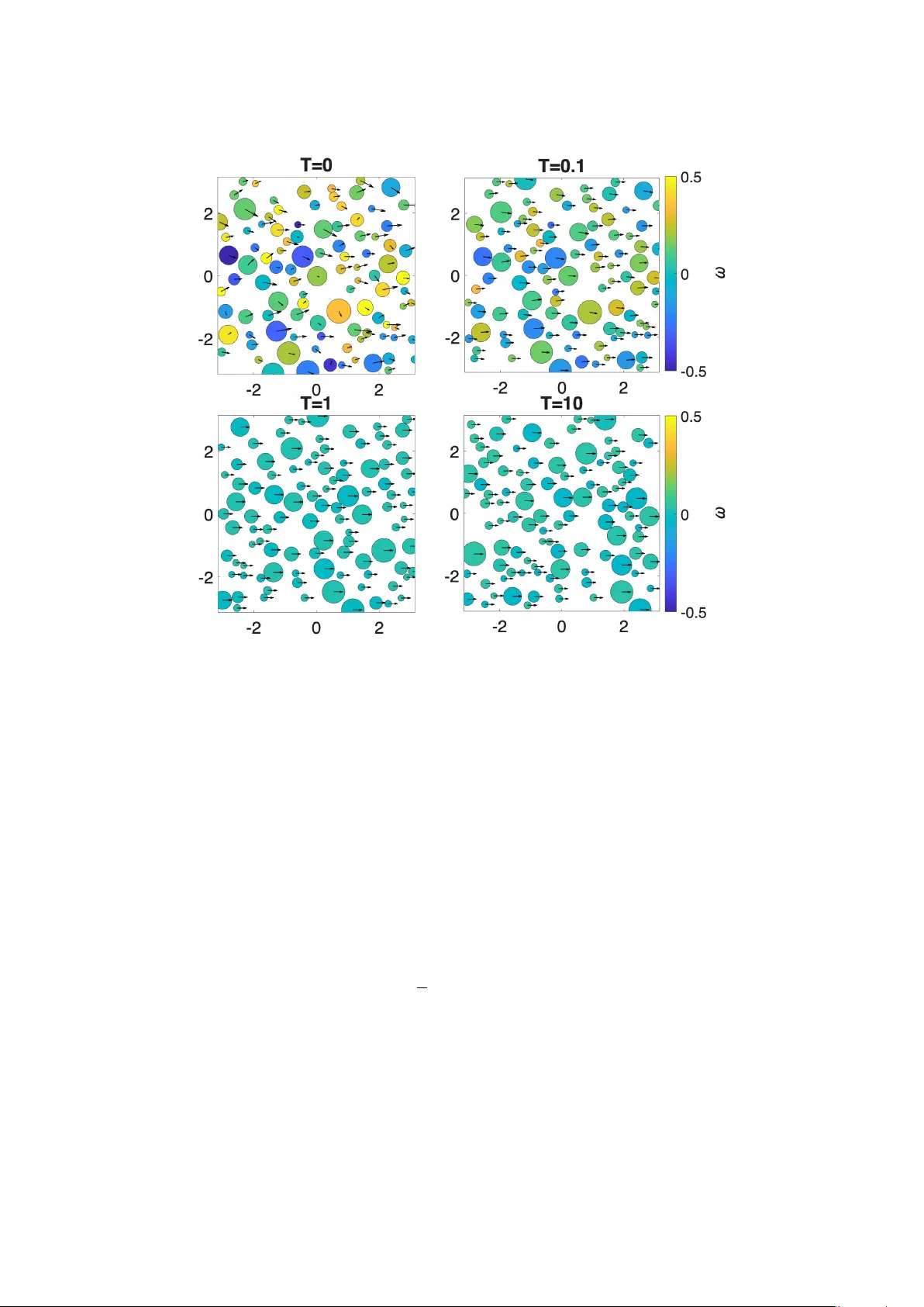
P article, kinetic and h ydro dynamic mo dels for sea ice flo es. P art I I: Rotating flo es with nonlinear con tact forces Quanling Deng ∗ Seung-Y eal Ha † Jaemo on Lee ‡ Abstract This paper extends the multiscale mo deling framew ork in tro duced in P art I (Deng and Ha, Physic a D: Nonline ar Phenomena 483 (2025) 134951 ) for sea-ice flo e dynamics with non-rotating flo es to the case with rotational flo es and nonlinear con tact interactions. Building on the particle–kinetic–hydrodynamic hierarc hy de- v elop ed for non-rotating flo es, w e generalize the particle model to describe ice flo es as rigid b odies characterized by p osition, linear velocity , angular velocity , size, and momen t of inertia. The interaction rules now include nonlinear contact forces and torques arising from short-range compression, restitution, and tangential friction la ws, together with hydrodynamic drag that couples translational and rotational motions. These particle descriptions lead to an enriched Vlasov-t yp e kinetic equa- tion p osed on an extended phase space, whose momen ts yield a hydrodynamic sys- tem for mass, momentum, and angular-momentum balances. Compared with Part I, the resulting macroscopic equations feature additional stress contributions, ro- tational transp ort, and dissipative mechanisms stemming from nonlinear collisions. The prop osed framew ork pro vides a more realistic description of sea-ice flo e dynam- ics and offers a systematic pathw a y to ward mu ltiscale mo deling of sea-ice rheology under complex environmen tal forcing. Keyw ords: Sea ice flo e dynamics, Hertz con tact mechanics, energy dissipation, mean- field approximation, hydrodynamic limit. 1 In tro duction Sea ice pla ys a fundamental role in Earth’s p olar climate system by regulating heat ex- c hange, momentum transfer, and biogeo c hemical pro cesses at the o cean–atmosphere in- terface. Its dynamics emerge from the complex in terplay b et w een environmen tal forcing, including wind, o cean currents, and wa v es, and mec hanical interactions among hetero- geneous flo es (c.f., [1, 2, 7, 27, 46, 55, 58, 61]). In the Marginal Ice Zone (MIZ), where ∗ Y au Mathematical Sciences Cen ter, Tsingh ua Univ ersity , Beijing, 100084, China (qldeng@tsingh ua.edu.cn); Sc ho ol of Computing, Australian National Univ ersity , Canberra, ACT 2601, Australia (quanling.deng@an u.edu.au). † Departmen t of Mathematical Sciences and Researc h Institute of Mathematics, Seoul National Uni- v ersity , Seoul 08826, Republic of Korea (syha@sn u.ac.kr). ‡ Departmen t of Mathematical Sciences, Seoul National Universit y , Seoul 08826, Republic of Korea (dlw oans0001@snu.ac.kr). 1 the ice co ver is highly fragmen ted, individual floe-flo e in teractions dominate the mec han- ical b eha vior of the ice pack, often giving rise to phenomena that are more naturally describ ed by particle flo es (c.f., [5, 6]). Con tinuum-based mo dels, suc h as elastic-plastic [16], viscous–plastic [42, 63], elastic– viscous–plastic [45], and Maxwell-t yp e rheological mo dels [19], hav e b een developed for sim ulating the large-scale b eha vior of compact ice packs (for ice sheets and glaciers, w e refer to, e.g., [57]). How ev er, the con tinuum assumption can break do wn in both large and small scales in the MIZ or other areas [68], where collisions, heterogeneity , and anisotropic deformation fields pro duce granular-lik e b eha vior that cannot b e adequately represen ted by homogenized constitutive laws. These limitations ha ve motiv ated the dev elopment of particle-based (discrete element) approaches [4, 18, 20, 43, 52, 54, 69], whic h explicitly represent sea ice as a collection of rigid b o dies and naturally capture pro cesses suc h as collisions, ridging, rafting, and fracture patterns. In earlier model dev elopments, Gudko vic h et al. [34] studied the dynamics of an individual flo e in 1963, based on the observ ations of Nansen [56] in 1902, and developed a mo del to describ e the sp eed and direction of drift dep ended on flo e size and shape. F uture directions for sea ice mo delling are also discussed here [7, 29, 47]. A key challenge in particle-based mo deling lies in accurately representing con- tact interactions. Nonlinear contact mec hanics, including Hertzian-type normal forces, v elo cit y-dep enden t restitution, tangen tial friction la ws, and torque transfer at con tact p oin ts, play a critical role in determining floe tra jectories and rotational dynamics. Such nonlinear collision mo dels, widely used in gran ular and rigid-b o dy sim ulations [17, 48], ha ve recently been applied to sea ice flo es [38]. Rotational degrees of freedom further enric h the dynamics: collisions generate torques, frictional impulses mo dify angular mo- men tum, and o cean drag acts sim ultaneously on translational and rotational motions. These effects contribute to complex b eha viors such as spin alignment, rotational cluster- ing, collision-induced jamming, and enhanced dissipation, all observ ed in high-resolution DEM studies [38]. In Part I of this series [23], w e ha v e dev elop ed a particle–kinetic–h ydro dynamic hierarc hy for non-rotating cylindrical flo es go verned b y linear contact forces. That form ulation established a systematic path wa y from Newtonian-type particle models to Vlaso v-type kinetic descriptions and further to hydrodynamic equations based on veloc- it y moments. While the non-rotating framework provides conceptual clarit y , it neglects nonlinear contact mechanics and rotational effects that are essential for accurately cap- turing sea-ice b eha vior in fragmented regimes. The present pap er extends the multiscale framew ork of P art I by incorp orating ro- tational degrees of freedom and nonlinear con tact forces into the particle, kinetic, and h ydro dynamic descriptions. This provides a pathw a y to couple particle and contin uum mo dels within a m ultiscale framew ork [24], together with their in tegration in to data assimilation schemes [14, 15, 21], enabling more accurate predictions. At the particle lev el, eac h floe is mo deled as a rigid bo dy c haracterized b y its position, orientation, linear v elo cit y , angular velocity , size, and moment of inertia. Collisions generate b oth forces and torques, describ ed through physically realistic nonlinear force la ws and frictional 2 in teractions. This leads to a richer kinetic formulation defined on an extended phase space that includes angular velocities and orien tations. Suitable moment closures then yield hydrodynamic equations that track mass, linear momentum, and angular momen- tum, together with stress and couple-stress con tributions arising from torque-generating in teractions. The ob jective of this Part I I work is to establish a rigorous theoretical foundation for such a rotating particle–kinetic–h ydro dynamic hierarch y . Our main con- tributions include: • a rigorous study on the b eha vior of total momen tum and energy of a particle model for rotating flo es with nonlinear contact forces; • the deriv ation of a kinetic mo del on an extended phase space incorp orating rota- tional dynamics, follo wed by a study on the momen tum and energy; • the developmen t and study of a hydrodynamic system that captures macroscopic ev olution of b oth linear and angular momen tum and energies. The rest of the pap er is organized as follo ws. In Section 2, w e in tro duce the rotating sea-ice flo e particle m odel with nonlinear contact laws in Subsection 2.1, follo wed by a study on the asymptotic b eha vior of total momentum and energy in Subsection 2.2. In Section 3 and Section 4, w e presen t the corresp onding kinetic description using the mean- field limit, follow ed by a hydrodynamic mo del with monokinetic closure. W e also study the asymptotic b eha vior on momentum and energies of these mo dels. In Section 5, we pro vide sev eral n umerical examples to v alidate our theoretical findings. Finally , Section 6 is dev oted to the summary of the pap er with a discussion of the main findings and future directions. 2 P article description for ice flo es In this section, we introduce the particle mo del for the ice flo es with rotation and non- linear Hertzian con tact forcing, follow ed by a study on its asymptotic collectiv e b eha vior on momentum and energy . 2.1 The particle mo del Consider colliding ice flo es with the geometry of cylinders. Given a system of n flo es, we denote b y r i the radius and h i the thic kness (or height) of the i -th flo e with i ∈ [ n ] := { 1 , 2 , · · · , n } . The radius and thickness c haracterize the flo e size. In a realistic sea ice flo e setting (particularly in marginal ice zones), the flo e size often follow a p o wer la w distribution [64], while the floe thickness distribu tion follows a Gamma distribution (see, for example, [11, 65, 66] for the Arctic region and [67] for the Antarctic region). The mass of the i -th flo e is m i = ρ ice π ( r i ) 2 h i , where the constant ρ ice is the density of sea ice flo es. W e assume that the mass of each flo e does not change o ver time (th us, no melting, freezing, or fracturing). W e denote by I i = m i ( r i ) 2 the momen t of inertia. The flo e p osition is denoted by x i = ( x i , y i ) T and the flo e velocity is v i = ( u i , v i ) T . W e denote 3 the flo e angular lo cation as θ i and angular velocity as ω i ˆ z . Herein, ˆ z is the unit vector along the z -axis (p erp endicular to the ( x, y ) plane). W e consider the angular velocity as a scalar in this dimension and omit the multiplication of ˆ z for simplicity . Thus, if the result of the cross pro duct is a v ector along the z -axis, w e consider it as a z -v alue scalar as in (2.1b) and (2.1d) b elo w. Lastly , let u o = u o ( x, y ) b e the giv en o cean surface v elo cit y . The gov erning equations of rotating-colliding sea ice flo e dynamics are giv en b y Newton’s equations: d x i d t = v i , i ∈ [ n ] , (2.1a) d θ i d t = ω i , (2.1b) m i d v i d t = 1 n n X j =1 ( f ij n + f ij t ) + α i  u i o − v i    u i o − v i   := F i , (2.1c) I i d ω i d t = 1 n n X j =1 ( r i n ij × f ij t ) + β i  ∇ × u i o / 2 − ω i    ∇ × u i o / 2 − ω i   := T i , (2.1d) where | · | is the ℓ 2 -norm and f ij n =  κ ij 1 δ ij + κ ij 2 ( v i − v j ) · n ij  n ij , f ij t = ζ ij ˜ f ij t , ˜ f ij t = κ ij 3 σ ij t ij , κ ij 1 = π E e χ ij h ij e g δ ij r ij e 2( h ij e ) 2 ! , g ( ξ ) = 0 . 9117 ξ 2 − 0 . 2722 ξ + 0 . 003324 ξ 2 − 1 . 524 ξ + 0 . 03159 κ ij 2 = η q 5 κ ij 1 m ij e , κ ij 3 = 6 G e E e κ ij 1 , (2.2) δ ij = d ij − ( r i + r j ) , with d ij = | x i − x j | , σ ij t = d σ ij d t = ( v j − v i ) · t ij − r j ω j − r i ω i , σ ij = Z t t start σ ij t ( s )d s = t ij c σ ij t , t ij c ≈ 2 . 94  m ij e κ ij 1  2 / 5 | v i − v j | − 1 / 5 , α i = π ρ o (2 C v ,o r i · D i + C h,o ( r i ) 2 ) , β i = π ( r i ) 4 ρ o ( C v ,o D i + r i C h,o / 5) . W e discuss the physical quan tities and parameters one by one b elo w. First, E e = E 2(1 − ν 2 ) , G e = E 4(2 + ν )(1 − ν ) , (2.3) where E is Y oung’s mo dulus, and ν is P oisson’s ratio (assuming the same for all flo es). In the integration for σ ij , t start sp ecifies the starting time of the collision, and t ij c is 4 an approximate contact duration time that comp ensates the in tegration [35]. χ is a c haracteristic function χ ij = ( 1 , when i  = j and δ ij < 0 , 0 , otherwise , (2.4) whic h characterizes whether flo es i and j are in contact or not. W e m ultiply this by κ ij 1 for notational simplicity . f ij n and f ij t are normal and tangential comp onen ts of the con tact force, resp ectiv ely . F or notational conv enience, we denote f ij c = f ij n + f ij t with the auxiliary parame ter ζ defined as ζ ij =    1 , when | ˜ f ij t | ≤ µ | f ij n | , µ | f ij n | | ˜ f ij t | , otherwise . (2.5) This imp oses the Coulomb friction law that plays an imp ortant role in limiting the tangen tial contact force relative to the magnitude of the normal contact force [43]: | f ij t | ≤ µ | f ij n | , where µ is the co efficien t of friction that c haracterizes the condition of the surfaces of t wo flo es in contact. W e assume zero tangen tial damping as in [17, 18]. The flo e contact force F i and torque T i are non-zero only when tw o flo es are in contact, i.e., δ ij < 0. W e also remark that for δ ij < 0, we hav e ξ < 0 and g ( ξ ) > 0. This guaran tees the correct sign of κ ij 1 δ ij in the term f ij n . W e follow the Hertz contact theory [41, 60] and adopt the mo del for the normal contact force (see the supplemen tary material of [38]). By default, i  = j, i, j ∈ [ n ]. W e assume δ ij = 0 when i = j (hence, f ij n = f ij t = 0 ) for notational simplicit y . σ ij t is the slip-rate along the tangen tial direction caused by b oth translation and rotation (relativ e contact velocity pro jected in the tangential direction). σ is the rotational deformation, i.e., the tangential shear deformation. ρ o is o cean density , D i is the ice-flo e draft (the part of the ice flo e b elow the water surface), C v ,o is o cean vertical drag co efficien ts, C h,o is o cean horizon tal drag co efficien ts. In default, we set D i = 0 . 9 h i . The vector n ij := x j − x i | x j − x i | is the unit normal vector p oin ting from the center of flo e i to flo e j (if i = j , let it b e z ), t ij is the unit vector along the tangential direction (rotating n ij coun terclo c kwise b y 90 ◦ ), r j is the radius multiplied by the asso ciated normal vector p oin ting tow ards the cen ter of the j -th flo e, E e is the effective contact mo dulus, h ij e := min { h i , h j } is the effectiv e con tact thickness (part of the thickness in con tact), m ij e := m i m j m i + m j is the effectiv e mass, r ij e := r i r j r i + r j is the effectiv e radius, and η := ln e r p ln 2 e r + π 2 < 0 . (2.6) Here e r is the restitution co efficien t in [0 , 1). The restitution co efficien t for ice flo es is a measure of kinetic energy loss during flo e collisions. The co efficien t is usually a p ositiv e 5 real n umber b et ween 0 and 1. A v alue of 0 indicates a p erfectly inelastic collision, while a v alue of 1 indicates a p erfectly elastic collision. The typical v alues of e r for sea ice are b et ween 0.1 and 0.3; see [51]. In ice floe studies, v alues betw een 0 and 1 are often emplo yed; see, for example [40]. Details are referred to equations (1), (8), (20), and (26) in the supplementary material of [38]. W e scale the summation of the con tact force by the factor of 1 /n to apply the mean-field theory for deriving the kinetic and h ydro dynamic mo dels. F or a system with a fixed num b er of flo es, this scaling factor ma y b e understo od as a factor of the mass and drag co efficien t. 2.2 Asymptotic b eha vior T o study the asymptotic b eha vior of the particle mo del (2.1), w e first define the strain and kinetic energies. The normal strain energy for t wo colliding flo es is defined as M ij 2 , x := Z δ ij 0 f ij n ,s d s = Z δ ij 0 κ ij 1 ( s ) s d s. This normal strain energy ev olves with resp ect to time. Using the Leibniz integral rule, w e hav e d M ij 2 , x d t = d d t Z δ 0 κ ij 1 ( s ) s d s = κ ij 1 ( δ ij ) δ ij d δ ij d t . (2.7) With this in mind, we define the flo e moments as follo ws: M 0 = n X i =1 m i , M 1 , v = n X i =1 m i v i , M 1 ,ω = n X i =1 ( m i x i × v i + I i ω i ) , M 2 = M 2 , v + M 2 , x + M 2 ,ω , M 2 , v = 1 2 n X i =1 m i | v i | 2 , M 2 , x = 1 2 n n X i,j =1 M ij 2 , x , M 2 ,ω = 1 2 n X i =1 I i ( ω i ) 2 , (2.8) where M 0 is the zero-order moment, i.e., total mass. M 1 , v is the total momentum. M 1 ,ω is the total angular momentum, which includes the orbital angular momentum (due to translational motion) and the spin angular momentum (due to rotation ab out the cen ter of mass). M 2 , x , M 2 , v , M 2 ,ω , and M 2 represen t the total normal strain e nergy , the total translational kinetic energy , the total rotational kinetic energy , and the total energy , resp ectiv ely . The scaling 1 n in M 2 , x ensures that total strain energy remain O (1) in the mean-field limit as n → ∞ . Note that each energies are b y definition p ositiv e. Lemma 2.1 (T otal momentum balances) . L et ( x i , v i , θ i , ω i ) b e a glob al solution to the system (2.1) . Then, the fol lowing assertions hold. 1. The total line ar momentum satisfies d M 1 , v d t = n X i =1 α i  u i o − v i    u i o − v i   . (2.9) 6 2. The total angular momentum satisfies d M 1 ,ω d t = n X i =1  α i x i ×  u i o − v i    u i o − v i   + β i  ∇ × u i o / 2 − ω i    ∇ × u i o / 2 − ω i    . (2.10) Pr o of. F or the first assertion, we first note that the relations δ ij = δ j i , n ij = − n j i , t ij = − t j i , i, j ∈ [ n ] , to see the anti-symmetry of the flo e-flo e contact force: f ij n = − f j i n , f ij t = − f j i t , i, j ∈ [ n ] . (2.11) No w, we use (2.1), (2.8), and (2.11) to find d M 1 , v d t = d d t n X i =1 m i v i = n X i =1 m i d v i d t = n X i =1  1 n n X j =1 ( f ij n + f ij t ) + α i  u i o − v i    u i o − v i    = 1 n n X i,j =1 ( f ij n + f ij t ) + n X i =1 α i  u i o − v i    u i o − v i   = n X i =1 α i  u i o − v i    u i o − v i   . F or the second claim, using (2.1) and the prop ert y of the cross pro duct v i × v i = 0, w e calculate d M 1 ,ω d t = d d t n X i =1 ( m i x i × v i + I i ω i ) = n X i =1  m i d x i d t × v i + m i x i × d v i d t + I i d ω i d t  = n X i =1  x i × m i d v i d t + I i d ω i d t  = n X i =1  x i ×  1 n n X j =1 ( f ij n + f ij t ) + α i  u i o − v i    u i o − v i    +  1 n n X j =1 ( r i n ij × f ij t ) + β i  ∇ × u i o / 2 − ω i    ∇ × u i o / 2 − ω i     =: T a + T b , where T a = 1 n n X i,j =1  x i × ( f ij n + f ij t ) + ( r i n ij × f ij t )  , T b = n X i =1  α i x i ×  u i o − v i    u i o − v i   + β i  ∇ × u i o / 2 − ω i    ∇ × u i o / 2 − ω i    . 7 W e denote the contact p oin t of flo es i and j as c ij . Then w e hav e c ij = x i + r i n ij , c j i = x j + r j n j i , c ij = c j i . (2.12) Using (2.12), anti-symmetry , and ( x i − x j ) × n ij = 0, w e calculate T a = 1 n n X i,j =1 x i × f ij n + 1 n n X i,j =1  x i × f ij t + ( r i n ij × f ij t )  = − 1 n n X i,j =1 x j × f ij n + 1 n n X i,j =1 c ij × f ij t = 1 2 n n X i,j =1 ( x i − x j ) × f ij n + 1 2 n n X i,j =1  c ij × f ij t + c j i × f j i t  = 0 . (2.13) This leads to the desired result for the balance law of total angular momentum. Remark 2.2. In the deriv ation of (2.13), w e used the con tact p oin t assumption/equalit y (2.12), whic h implies δ ij = 0. This distinguishes it from the contact deformation assump- tion for computing the normal con tact force. That is, we assume that the flo e particles deform up on contact, and the ov erlap (deformation) δ ij is used to compute the contact forces f ij n and f ij t . How ever, when computing torques, w e assume that the contact o c- curs at a p oin t lo cated on the undeforme d ge ometry , i.e., at a distance r i n ij from the cen ter. This introduces a mo deling appro ximation, which is justified in [53, 59]: 1. Deformations are small: In most sea ice flo e particle settings, ov erlaps are v ery small compared to particle size, so undeformed geometry in tro duces only second- order errors. 2. Appro ximate consistency: The total torque from eac h force pair cancels under Newton’s third la w, ensuring conserv ation of angular momentum. Lemma 2.3 (T otal energy balance) . L et ( x i , v i , θ i , ω i ) b e a glob al solution to system (2.1) . Then, the fol lowing r elation holds: d M 2 d t = 1 2 n n X i,j =1 κ ij 2 | ( v i − v j ) · n ij | 2 − 1 2 n n X i,j =1 ζ ij κ ij 3 t ij c ( σ ij t ) 2 + n X i =1 α i  u i o − v i    u i o − v i   · v i + n X i =1 β i ω i  ∇ × u i o / 2 − ω i    ∇ × u i o / 2 − ω i   . (2.14) 8 Pr o of. W e take the pro duct of (2.1c) with v i , and sum up the resulting equations ov er all i ∈ [ n ] to obtain d M 2 , v d t = n X i =1 m i d v i d t · v i = n X i =1  1 n n X j =1 ( f ij n + f ij t ) + α i  u i o − v i    u i o − v i    · v i = 1 n n X i,j =1  κ ij 1 δ ij + κ ij 2 ( v i − v j ) · n ij  n ij · v i + 1 n n X i,j =1 f ij t · v i + n X i =1 α i  u i o − v i    u i o − v i   · v i =: T 11 + T 12 + T 13 + n X i =1 α i  u i o − v i    u i o − v i   · v i . (2.15) Belo w, w e estimate the terms T 1 i , i = 1 , 2 , one by one. F or T 13 , we estimate it combined with the angular velocity comp onen t afterwards. • Case A.1: W e use (2.1a) and the relations: δ ij = δ j i , n ij = − n j i to rewrite T 11 = 1 n n X i,j =1 κ ij 1 δ ij n ij · d x i d t = − 1 n n X i,j =1 κ ij 1 δ ij n ij · d x j d t = − 1 2 n n X i,j =1 κ ij 1 δ ij n ij · d( x j − x i ) d t = − 1 2 n n X i,j =1 κ ij 1 δ ij · d δ ij d t = − d M 2 , x d t , (2.16) where we used (2.7) and the following identit y: d δ ij d t = d d t  | x i − x j | − ( r i + r j )  = d d t q ( x j − x i ) 2 + ( y j − y i ) 2 = 2( x j − x i )d( x j − x i ) + 2( y j − y i )d( y j − y i ) 2 p ( x j − x i ) 2 + ( y j − y i ) 2 d t = n ij · d( x j − x i ) d t . • Case A.2: Similarly , we ha ve T 12 = 1 n n X i,j =1 κ ij 2  ( v i − v j ) · n ij  n ij · v i = − 1 n n X i,j =1 κ ij 2  ( v i − v j ) · n ij  n ij · v j = 1 2 n n X i,j =1 κ ij 2  ( v i − v j ) · n ij  2 . (2.17) 9 F or rotational kinetic energy , we take an inner pro duct of (2.1d) with ω i , and sum up the resulting equations ov er all i ∈ [ n ] to get d M 2 ,ω d t = n X i =1 I i d ω i d t · ω i = n X i =1  1 n n X j =1 ( r i n ij × f ij t ) + β i  ∇ × u i o / 2 − ω i    ∇ × u i o / 2 − ω i    · ω i = 1 n n X i,j =1 r i n ij × f ij t ω i + n X i =1 β i ω i  ∇ × u i o / 2 − ω i    ∇ × u i o / 2 − ω i   =: T 14 + n X i =1 β i ω i  ∇ × u i o / 2 − ω i    ∇ × u i o / 2 − ω i   . (2.18) Using the definition (2.2) and the facts that n ij × t ij = 1 and t ij · t ij = 1, we now calculate T 1 , 3 + T 1 , 4 b elo w: T 1 , 3 + T 1 , 4 = 1 n n X i,j =1 f ij t · v i + 1 n n X i,j =1 n ij × f ij t r i ω i = − 1 n n X i,j =1 f ij t · v j + 1 n n X i,j =1 n ij × f ij t r j ω j = 1 2 n n X i,j =1 f ij t · ( v i − v j ) + 1 2 n n X i,j =1 n ij × f ij t ( r i ω i + r j ω j ) = 1 2 n n X i,j =1 f ij t ·  ( v i − v j ) · t ij  t ij + 1 2 n n X i,j =1 f ij t · ( r i ω i + r j ω j ) t ij = − 1 2 n n X i,j =1 f ij t · σ ij t t ij = − 1 2 n n X i,j =1 ζ ij κ ij 3 t ij c ( σ ij t ) 2 . (2.19) Summing up the abov e estimates in (2.15) with terms (2.16), (2.17), and (2.18) with term (2.19) giv es the desired estimate for the total energy . Lemma 2.4 (T otal energy low er b ound) . L et ( x i , v i , θ i , ω i ) b e a glob al solution to the system (2.1) . Assume a uniform b ound on the dur ation of c ontact time, i.e., t ij c < t max c . If α i = β i = 0 , ∀ i ∈ [ n ] , then ther e exist p ositive c onstants A 0 and A 1 such that M 2 ( t ) ≥ M 2 (0) e − A 0 t + A 1 A 0 | M 1 , v (0) | 2  1 − e − A 0 t  . 10 Pr o of. With α i = β i = 0 , ∀ i ∈ [ n ] , the equalities (2.9) and (2.10) reduce to d M 1 , v d t = 0 , d M 1 ,ω d t = 0 (2.20) while the relation (2.14) reduces to d M 2 d t = 1 2 n n X i,j =1 κ ij 2 | ( v i − v j ) · n ij | 2 − 1 2 n n X i,j =1 ζ ij κ ij 3 t ij c ( σ ij t ) 2 . Using the definition (2.2), the fact κ ij 2 < 0 (since η < 0 as in (2.6)), and the positivity of the other parameters, we observe d M 2 d t ≤ 0 , i.e., total energy is dissipative. No w, w e use the Cauch y–Sc hw arz inequality and boundedness of the mass of flo e particles to see that there exist p ositiv e constan ts as the flo e particle radii, thickness, and masses are fixed for a fixed s ystem with n flo es such that 1 2 n n X i,j =1 | κ ij 2 |  ( v j − v i ) · n ij  2 ≤ 1 2 n κ max 2 n X i,j =1 | v j − v i | 2 ≤ κ max 2 2 nm 2 min n X i,j =1 m i m j | v j − v i | 2 = κ max 2 2 nm 2 min n X i,j =1 m i m j  | v j | 2 + | v i | 2 − 2 v i · v j  ≤ κ max 2 2 nm 2 min  2 nm max n X i =1 m i | v i | 2 − 2    n X i =1 m i v i    2  = κ max 2 m max m 2 min n X i =1 m i | v i | 2 − κ max 2 nm 2 min    n X i =1 m i v i    2 := T 21 − T 22 , (2.21) where κ max 2 = max i,j | κ ij 2 | and m min = min i m i , m max = max i m i . By definition, w e b ound T 21 T 21 = 2 κ max 2 m max m 2 min M 2 , v ≤ 2 κ max 2 m max m 2 min M 2 . (2.22) 11 W e use (2.20) to see T 22 = κ max 2 nm 2 min | M 1 , v (0) | 2 . (2.23) T o b ound the term 1 2 n P n i,j =1 ζ ij κ ij 3 t ij c ( σ ij t ) 2 , we recall σ ij t = ( v j − v i ) · t ij − r j ω j − r i ω i , | t ij | = 1 . Using ( a + b + c ) 2 ≤ 3( a 2 + b 2 + c 2 ) and | ( v j − v i ) · t ij | ≤ | v j − v i | , ( σ ij t ) 2 ≤ 3  | v j − v i | 2 + ( r j ω j ) 2 + ( r i ω i ) 2  . With κ ij 3 ≤ κ max 3 := max i,j κ ij 3 and 0 ≤ ζ ij ≤ 1 by (2.5), w e then hav e n X i,j =1 ζ ij κ ij 3 t ij c ( σ ij t ) 2 ≤ κ max 3 t max c n X i,j =1 ( σ ij t ) 2 ≤ 3 κ max 3 t max c n X i,j =1  | v j − v i | 2 + ( r j ω j ) 2 + ( r i ω i ) 2  . (2.24) W e use n X i,j =1 | v j − v i | 2 = 2 n n X i =1 | v i | 2 − 2    n X i =1 v i    2 ≤ 2 n n X i =1 | v i | 2 , and n X i,j =1  ( r j ω j ) 2 + ( r i ω i ) 2  = 2 n n X i =1 ( r i ω i ) 2 . W e substitute into (2.24) to find n X i,j =1 ζ ij κ ij 3 t ij c ( σ ij t ) 2 ≤ 6 nκ max 3 t max c  n X i =1 | v i | 2 + n X i =1 ( r i ω i ) 2  . (2.25) Similarly , we ha ve M 2 , v = 1 2 n X i =1 m i | v i | 2 ≥ m min 2 n X i =1 | v i | 2 ⇒ n X i =1 | v i | 2 ≤ 2 m min M 2 , v . Moreo ver I i = m i ( r i ) 2 ≥ m min ( r i ) 2 , hence w e hav e I i ( ω i ) 2 ≥ m min ( r i ω i ) 2 = ⇒ n X i =1 ( r i ω i ) 2 ≤ 1 m min n X i =1 I i ( ω i ) 2 = 2 m min M 2 ,ω . W e put these into (2.25) to get 1 2 n n X i,j =1 ζ ij κ ij 3 t ij c ( σ ij t ) 2 ≤ 6 κ max 3 t max c m min  M 2 , v + M 2 ,ω  ≤ 6 κ max 3 t max c m min M 2 . 12 Finally , we com bine (2.24) with (2.21), (2.22) and (2.23) to obtain d M 2 d t ≥ −  2 κ max 2 m max m 2 min + 6 κ max 3 t max c m min  M 2 + κ max 2 nm 2 min | M 1 , v (0) | 2 =: − A 0 M 2 + A 1 | M 1 , v (0) | 2 . W e use Gr¨ on wall’s lemma [26, 33] to find the desired estimate. Remark 2.5. Similar to the result [36] for the Cuck er-Smale mo del, if the drag force is absen t (i.e., α i = β i = 0), Lemma 2.3 and Lemma 2.4 imply that the total energy M 2 is monotonically decreasing with a low er b ound. Lemma 2.4 uses an assumption on the duration of con tact t ij c . This is due to that the unregularized formul a t ij c ∼ | v i − v j | − 1 / 5 in (2.2) is not uniformly b ounded as | v i − v j | → 0. T o obtain an energy-type estimate b ound, one needs to remo ve this singularit y . The common flo e modeling practice [18, 38]: either (i) caps t ij c b y a prescrib ed maximal contact time (often tied to time-step size dt in numerical simulation); or (ii) regularizes with a small v ∗ > 0 as t ij c := 2 . 94  m ij e κ ij 1  2 / 5  | v i − v j | + v ∗  − 1 / 5 , v ∗ > 0 . On the other hand, Coulom b friction la w imp osed through ζ ij also k eeps the term P n i,j =1 ζ ij κ ij 3 t ij c ( σ ij t ) 2 from unbounded. W e now consider a sp ecial case where the o cean v elo cit y is constant. In such a case, w e sho w that the particle translational and rotational v elo cities are conv erging to constants. T o establish this result rigorously , we first recall Barbalat’s lemma to be used in later sections. It claims that if a uniformly con tinuous function is (Riemann)- in tegrable on the p ositiv e real line, then it conv erges to 0, as t go es to infinity . Lemma 2.6 (Barbalat’s Lemma) . Supp ose that f : R + → R is a uniformly c ontinuous function. If Z ∞ 0 f ( t )d t < ∞ , = ⇒ lim t →∞ f ( t ) = 0 . Theorem 2.7. Supp ose that the given o c e an surfac e velo city is c onstant: u i o = u ∞ o : c onstant , ∀ i ∈ [ n ] , and let ( x i , v i , θ i , ω i ) b e a glob al solution to system (2.1) . If α i , β i > 0 , we have lim t →∞ ∥ v i − u ∞ o ∥ = 0 , lim t →∞ ω i ( t ) = 0 , ∀ i ∈ [ n ] . Pr o of. Due to the translational inv ariance of system (2.1), we ma y assume that u ∞ o ≡ 0 13 and we claim that lim t →∞ v i ( t ) = 0 , lim t →∞ ω i ( t ) = 0 . (2.26) It follows from Lemma 2.3 that d M 2 d t ≤ − n X i =1 ( α i   v i   3 + β i   ω i   3 ) , (2.27) where the first tw o terms in the right-hand side of (2.14) are negativ e (since κ ij 2 < 0 , ζ κ ij 3 > 0). Th us, total energy is non-increasing, which leads to b oundedness of κ ij 1 δ ij , v i , and ω i since each energy M 2 , x , M 2 , v , M 2 ,ω b ecomes b ounded. Next, w e in tegrate inequality (2.27), Z ∞ 0 n X i =1 ( α i   v i   3 + β i   ω i   3 )d t ≤ M 2 (0) − inf t> 0 M 2 ( t ) ≤ M 2 (0) , to see that total energy is non-negativ e. Therefore, if w e sho w that v i and ω i are uniformly contin uous, w e can show that it tends to 0, by Barbalat’s Lemma 2.6. W e will pro ve it using the b oundedness of ˙ v i and ˙ ω i (since the time deriv ative of the in tegrand of the ab o v e integral is these terms multiplied b y b ounded terms). Recall m i d v i d t = 1 n n X j =1 ( f ij n + f ij t ) − α i v i   v i   , I i d ω i d t = 1 n n X j =1 ( r i n ij × f ij t ) − β i ω i   ω i   , Under the b oundedness of δ ij , one can easily show the b oundedness of κ i co efficien t terms and σ ij , which leads to the boundedness of righ t-hand-side of the ab o v e equations. Therefore, v i and ω i are uniformly con tinuous, which sho ws (2.26). 3 F rom particle to kinetic description In this section, w e first recall the formal deriv ation from the particle model to the kinetic mo del as the mean-field approximation of the particle mo del with n ≫ 1. W e assume that the n umber of particles in volv ed in the particle system (2.1) is sufficiently large so that it b ecomes meaningful to use the mean-field approximation via the one-particle distribution function to describ e the ov erall effective dynamics of the original system. 14 3.1 Kinetic mo del for ice flo e dynamics W e first rewrite the flo e particle mo del (2.1) as                      d x i d t = v i , d θ i d t = ω i , i ∈ [ n ] , d v i d t = 1 m i h 1 n n X j =1 ( f ij n + f ij t ) + α i  u i o − v i    u i o − v i   i =: F i m i , d ω i d t = 1 I i h 1 n P n j =1 ( r i n ij × f ij t ) + β i  ∇ × u i o / 2 − ω i    ∇ × u i o / 2 − ω i   i := T i I i dr i dt = 0 , dh i dt = 0 , (3.1) where we assume that the flo e sizes and thicknesses do not change in time. In what follo ws, w e adopt BBGKY hierarch y (Bogoliub o v–Born–Green–Kirkwoo d–Yv on, [8–10, 50, 70]) to derive a kinetic equation for the one-particle distribution function o ver the generalized phase space R 2 x × R 2 v × T × R ω × R + × R + ( T means 1D torus). In general, one assumes that the distribution function b elongs to a function class such that it is perio dic in the toroidal v ariables and rapidly decaying in the unbounded v ariables, ensuring that all b oundary terms arising from integration by parts v anish. • Step A (Deriv ation of the Liouville equation for the n -particle distribution function): First, we define n -particle distribution function on the n -particle phase space R 4 n × T n × R n × R 2 n + : F n = F n ( t, x 1 , v 1 , θ 1 , ω 1 , r 1 , h 1 , · · · , x n , v n , θ n , ω n , r n , h n ) , (3.2) for ( x i , v i , θ i , ω i , r i , h i ) ∈ R 2 × R 2 × T × R ω × R + × R + , i ∈ [ n ]. Note that the n -particle probability density function F n is symmetric in its phase v ariable in the sense that F n ( t, · · · , x i , v i , θ i , ω i , r i , h i , · · · , x j , v j , r j , h j , · · · ) = F n ( t, · · · , x j , v j , θ j , ω j , r j , h j , · · · , x i , v i , r i , h i , · · · ) . (3.3) Then, F n satisfies the Liouville equation on the generalized n -particle phase space: ∂ t F n + n X i =1 ∇ x i · ( ˙ x i F n ) + n X i =1 ∇ v i · ( ˙ v i F n ) + n X i =1 ∂ θ i ( ˙ θ i F n ) + n X i =1 ∂ ω i ( ˙ ω i F n ) + n X i =1 ∂ r i ( ˙ r i F n ) + n X i =1 ∂ h i ( ˙ h i F n ) = 0 , (3.4) where ∇ x i · ( ) and ∇ v i · ( ) denote the divergences in x i and v i -v ariables, resp ectiv ely . By using (3.1), the ab o ve system can also b e written as ∂ t F n + n X i =1 v i · ∇ x i F n + n X i =1 ∇ v i ·  F i m i F n  + n X i =1 ω i ∂ θ i F n + n X i =1 ∂ ω i  T i I i F n  = 0 . (3.5) 15 • Step B (Deriv ation of equation for the j -particle distribution function): F or notational simplicit y , we set z := ( x , v , θ , ω , r, h ) , d z j = d x j d v j d θ j d ω j d r j d h j , j ∈ [ n ] , d E n : j = n Y i = j +1 d z i . Then, we in tro duce the j -marginal distribution function F n : j b y the integration of (3.2): F n : j := Z R 4( n − j ) × T n − j × R n − j × R 2( n − j ) + F n d E n : j . Next, we derive an equation for F n : j . F or this, we rewrite (3.5) as follo ws. ∂ t F n = − j X i =1 ∇ x i · ( v i F n ) − j X i =1 ∇ v i ·  F i m i F n  − j X i =1 ∂ θ i ( ω i F n ) − j X i =1 ∂ ω i ( T i I i F n ) − n X i = j +1 ∇ x i · ( v i F n ) − n X i = j +1 ∇ v i ·  F i m i F n  − n X i = j +1 ∂ θ i ( ω i F n ) − n X i = j +1 ∂ ω i  T i I i F n  . (3.6) No w, set ˆ R = R 4( n − j ) × T n − j × R n − j × R 2( n − j ) + , and integrate the Liouville equation (3.6) ov er E n : j to obtain ∂ t F n : j = − j X i =1 Z ˆ R ∇ x i · ( v i F n )d E n : j − j X i =1 Z ˆ R ∇ v i ·  F i m i F n  d E n : j − j X i =1 Z ˆ R ∂ θ i ( ω i F n )d E n : j − j X i =1 Z ˆ R ∂ ω i  T i I i F n  d E n : j − n X i = j +1 Z ˆ R ∇ x i · ( v j F n )d E n : j − n X i = j +1 Z ˆ R ∇ v i ·  F i m i F n  d E n : j − n X i = j +1 Z ˆ R ∂ θ i ( ω i F n )d E n : j − n X i = j +1 Z ˆ R ∂ ω i  T i I i F n  d E n : j =: 8 X k =1 T 3 k . (3.7) Using the div ergence theorem and the deca y condition of F n at infinit y , it is easy to v erify the following identities: T 3 k = 0 , k = 5 , 6 , 7 , 8 . In the next lemma, we estimate the terms T 3 i , i = 1 , · · · , 4, one by one. F or simplicit y , we denote ˆ R 1 = R 4 × T × R × R 2 + . 16 Lemma 3.1. L et F n b e a glob al solution to (3.4) which de c ays to zer o sufficiently fast at infinity for al l phase variables. Then, we have the fol lowing identities: ( i ) T 31 = − j X i =1 v i · ∇ x i F n : j , T 33 = − j X i =1 ω i ∂ θ i F n : j , ( ii ) T 32 = − 1 n j X i =1 ∇ v i · h 1 m i j X k =1 f ik c  F n : j i − n − j n j X i =1 Z ˆ R 1 ∇ v i ·  1 m i f i ( j +1) c F n : j +1  d z j +1 − j X i =1 1 m i ∇ v i ·  α i  u i o − v i    u i o − v i   F n : j  , ( iii ) T 34 = − 1 n j X i =1 ∂ ω i  F n : j I i j X k =1 ( r i n ik × f ik t )  − n − j n j X i =1 Z ˆ R 1 ∂ ω i  F n : j +1 I i ( r i n i ( j +1) × f i ( j +1) t )  d z j +1 − j X i =1 1 I i ∂ ω i  β i  ∇ × u i o / 2 − ω i    ∇ × u i o / 2 − ω i   F n : j  . Pr o of. (i) With v ariable indep endence, w e exchange the deriv ative and integration to arriv e at T 31 = − j X i =1 Z ˆ R ∇ x i · ( v i F n )d E n : j = − j X i =1 ∇ x i · ( v i F n : j ) = − j X i =1 v i · ∇ x i F n : j . Similarly , we calculate T 33 = − j X i =1 Z ˆ R ∂ θ i ( ω i F n )d E n : j = − j X i =1 ω i ∂ θ i F n : j . 17 (ii) Now, we use (3.3) to see that T 32 = − j X i =1 Z ˆ R ∇ v i ·  F i m i F n  d E n : j = − 1 n j X i =1 Z ˆ R ∇ v i ·  F n m i n X k =1 f ik c  d E n : j − j X i =1 1 m i Z ˆ R ∇ v i ·  α i  u i o − v i    u i o − v i   F n  d E n : j = − 1 n j X i =1 Z ˆ R ∇ v i ·  F n m i j X k =1 f ik c  d E n : j − 1 n j X i =1 Z ˆ R ∇ v i ·  F n m i n X k = j +1 f ik c  d E n : j − j X i =1 1 m i ∇ v i ·  α i  u i o − v i    u i o − v i   F n : j  = − 1 n j X i =1 ∇ v i · h 1 m i j X k =1 f ik c  F n : j i − n − j n j X i =1 Z ˆ R 1 ∇ v i ·  1 m i f i ( j +1) c F n : j +1  d z j +1 − j X i =1 1 m i ∇ v i ·  α i  u i o − v i    u i o − v i   F n : j  . (iii) Similarly , we use (3.1), (3.3) and calculate T 34 = − j X i =1 Z ˆ R ∂ ω i  T i I i F n  d E n : j = − 1 n j X i =1 Z ˆ R ∂ ω i  F n I i n X k =1 ( r i n ik × f ik t )  d E n : j − j X i =1 1 I i Z ˆ R ∂ ω i  β i  ∇ × u i o / 2 − ω i    ∇ × u i o / 2 − ω i   F n  d E n : j = − 1 n j X i =1 ∂ ω i  F n : j I i j X k =1 ( r i n ik × f ik t )  − n − j n j X i =1 Z ˆ R 1 ∂ ω i  F n : j +1 I i ( r i n i ( j +1) × f i ( j +1) t )  d z j +1 − j X i =1 1 I i ∂ ω i  β i  ∇ × u i o / 2 − ω i    ∇ × u i o / 2 − ω i   F n : j  . 18 F or a fixed j , let n → ∞ and w e assume that the exists a limit F j suc h that lim n →∞ F n : j = F j in suitable sense . Then, in (3.7), we use Lemma 3.1 and formally as n → ∞ , the limit F j satisfies ∂ t F j + j X i =1 v i · ∇ x i F j + j X i =1 Z ˆ R 1 ∇ v i ·  1 m i f i ( j +1) c F j +1  d z j +1 + j X i =1 ω i ∂ θ i F j + j X i =1 Z ˆ R 1 ∂ ω i  F j +1 I i ( r i n i ( j +1) × f i ( j +1) t )  d z j +1 + j X i =1 1 m i ∇ v i ·  α i  u i o − v i    u i o − v i   F j  + j X i =1 1 I i ∂ ω i  β i  ∇ × u i o / 2 − ω i    ∇ × u i o / 2 − ω i   F j  = 0 . (3.8) Note that the dynamics of F j in (3.8) dep ends on F j +1 . In particular, for j = 1, w e remo ve the sup erscript for simplicity to arrive at ∂ t F + v · ∇ x F + ω ∂ θ F + α m ∇ v ·  ( u o − v ) | u o − v | F  + β I ∂ ω  ( ∇ × u o / 2 − ω ) |∇ × u o / 2 − ω | F  + Z ˆ R 1 ∇ v ·  1 m f 12 c F 2  d z 2 + Z ˆ R 1 ∂ ω  F 2 I ( r n 12 × f 12 t )  d z 2 = 0 . (3.9) • Step C (F ormal deriv ation of kinetic equation for one-particle distribution function): W e assume the “molecular chaos assumption” b y setting F 2 ( t, z , z ∗ ) = F ( t, z ) ⊗ F ( t, z ∗ ) . (3.10) Finally , we substitute the ansatz (3.10) in to (3.9) to get the kinetic equation for F : ∂ t F + v · ∇ x F + ω ∂ θ F + α m ∇ v ·  ( u o − v ) | u o − v | F  + β I ∂ ω  ( ∇ × u o / 2 − ω ) |∇ × u o / 2 − ω | F  + ∇ v · h Z ˆ R 1 1 m f 12 c F ( t, z ∗ )d z ∗  F ( t, z ) i + ∂ ω h Z ˆ R 1 1 I ( r n 12 × f 12 t ) F ( t, z ∗ )d z ∗  F ( t, z ) i = 0 . (3.11) 19 In what follo ws, we use handy notation: γ o := α m , γ b := β I , γ 1 := κ 1 m , γ 2 := κ 2 m , γ 3 := ζ κ 3 m , γ 4 := ζ κ 3 I , f [ F ] = f o + f c [ F ] , f o := γ o ( u o − v ) | u o − v | , f c [ F ] = f c, n [ F ] + f c, v [ F ] + f c, t [ F ] , f c, n [ F ]( t, z ) := Z ˆ R 1 γ 1 ( | x ∗ − x | − ( r + r ∗ )) n ( x , x ∗ ) F ( t, z ∗ )d z ∗ , f c, v [ F ]( t, z ) := Z ˆ R 1 γ 2 [( v − v ∗ ) · n ( x , x ∗ )] n ( x , x ∗ ) F ( t, z ∗ )d z ∗ , f c, t [ F ]( t, z ) := Z ˆ R 1 γ 3 σ t ( x , x ∗ ) F ( t, z ∗ )d z ∗ , f ω [ F ] = f ω ,o [ F ] + f ω ,t [ F ] , f ω ,o [ F ] = γ b ( ∇ × u o / 2 − ω ) |∇ × u o / 2 − ω | , f ω ,t [ F ]( t, z ) := Z ˆ R 1 γ 4 r σ F ( t, z ∗ )d z ∗ , (3.12) where the last integration used n ( x , x ∗ ) × t ( x , x ∗ ) = 1 . Note that γ i are all functions of the phase v ariables ( r , h, r ∗ , h ∗ ). Finally , we substitute (3.12) into (3.11) to arrive at the Vlasov-McKean equation: ∂ t F + v · ∇ x F + ω ∂ θ F + ∇ v · ( f [ F ] F ) + ∂ ω ( f ω [ F ] F ) = 0 . (3.13) W e remark that the final tw o terms on the left-hand side of (3.13) account for the in ternal stress within the flo e field due to contact interactions and the external forcing from o cean drag. 3.2 Macroscopic b eha vior of the kinetic mo del F rom now on, as long as there is no confusion, w e suppress t -dep endence in F . i.e., F ( z ) ≡ F ( t, z ) , z ∈ ˆ R 1 . F or simplicity , w e denote ˆ R 2 = R 8 × T 2 × R 2 × R 4 + . Next, we define the energy functional as follows.              E := E K + E P + E ω , E K := 1 2 Z ˆ R 1 m | v | 2 F ( z )d z , E ω := 1 2 Z ˆ R 1 I ω 2 F ( z )d z , E P := 1 2 Z ˆ R 2 Z δ ( z , z ∗ ) 0 ˜ κ 1 ( η ) η d η ! F ( z ) F ( z ∗ )d z d z ∗ , ˜ κ 1 ( δ ( z , z ∗ )) = κ 1 ( z , z ∗ ) . W e observe that each functional comp onen t in E is nonnegative, hence the energy func- tional E is nonnegative. In the following tw o lemmas, we establish the macroscopic b eha vior of the kinetic description of the flo e dynamics. 20 Lemma 3.2 (Macroscopic b eha vior) . L et F b e a glob al smo oth pr ob ability density solu- tion to system (3.13) which de c ays sufficiently fast at infinity in phase sp ac e. Then, the fol lowing estimates hold. ( i ) d d t Z ˆ R 1 mF ( t, z )d z = 0 . ( ii ) d d t Z ˆ R 1 m v F d z = Z ˆ R 1 α ( u o − v ) | u o − v | F ( t, z )d z . ( iii ) d d t Z ˆ R 1 ( m x × v + I ω ) F d z = Z ˆ R 1 α x × ( u o − v ) | u o − v | F ( t, z )d z + Z ˆ R 1 β ( ∇ × u o / 2 − ω ) |∇ × u o / 2 − ω | F ( t, z )d z . ( iv ) d E d t = Z ˆ R 1 α v · ( u o − v ) | u o − v | F ( z ) d z + Z ˆ R 1 β ω ( ∇ × u o / 2 − ω ) |∇ × u o / 2 − ω | F ( t, z ) d z + 1 2 Z ˆ R 2 κ 2 [( v − v ∗ ) · n ( x , x ∗ )] 2 F ( z ) F ( z ∗ )d z ∗ d z − 1 2 Z ˆ R 2 ζ κ 3 t c σ 2 t F ( z ) F ( z ∗ )d z ∗ d z . (3.14) Pr o of. (i) Note that d r d t = d h d t = 0 which implies d m d t = 0 . W e m ultiply (3.13) by m and integrate it ov er the phase space ˆ R 1 and use the decay of F at infinit y to find the conserv ation of total mass: d d t Z ˆ R 1 mF ( t, z )d z = 0 . (ii) Next, w e derive a balance law for momentum. F or this, w e multiply (3.13) by v to see that ∂ t ( v F ) + ∇ x ·  v ⊗ v F  + ∇ v ·  v ⊗ f [ F ] F  + ∂ θ ( ω v F ) + ∂ ω ( v f ω [ F ] F ) = f o F + f c [ F ] F . (3.15) Similarly , using an ti-symmetry , we multiply (3.15) b y m and integrate it o ver the phase space ˆ R 1 to find d d t Z ˆ R 1 m v F ( t, z )d z = Z ˆ R 1 m f o F d z + Z ˆ R 1 m f c [ F ] F d z = Z ˆ R 1 α ( u o − v ) | u o − v | F ( z )d z + Z ˆ R 2 m f c ( z , z ∗ ) F ( z ∗ ) F ( z )d z ∗ d z = Z ˆ R 1 α ( u o − v ) | u o − v | F ( z )d z − Z ˆ R 2 m f c ( z ∗ , z ) F ( z ∗ ) F ( z )d z ∗ d z = Z ˆ R 1 α ( u o − v ) | u o − v | F ( z )d z . 21 This gives the desired result. (iii) First, using the prop ert y of cross pro duct v × v = 0, we multiply (3.13) b y m x × v and integrate the resulting relation to find d d t Z ˆ R 1 ( m x × v ) F ( t, z )d z = − Z ˆ R 1 ( m x × v ) ∇ x ·  v F  d z − Z ˆ R 1 ( m x × v ) ∇ v ·  f [ F ] F  d z − Z ˆ R 1 ∂ θ ( mω ( x × v ) F )d z − Z ˆ R 1 ∂ ω ( m ( x × v ) f ω [ F ] F )d z = Z ˆ R 1 m v × v F d z + Z ˆ R 1 m x × f [ F ] F d z = Z ˆ R 1 m x × f o F d z + Z ˆ R 1 m x × ( f c, n [ F ] + f c, v [ F ] + f c, t [ F ]) F d z = S 1 + S 21 + S 22 + S 23 . Next estimate S 1 and S 2 i , i = 1 , 2 one by one. • (Estimation of S 1 ): W e use the functional form of f o in (3.12). S 1 = α Z ˆ R 1 x × ( u o − v ) | u o − v | F ( t, z )d z . • (Estimation of S 2 , i = 1 , 2): W e use anti-symmetry of the in tegrand under the trans- formation z ↔ z ∗ to get S 21 = Z ˆ R 2 mγ 1 ( | x ∗ − x | − ( r + r ∗ )) ( x × n ( x , x ∗ )) F ( t, z ∗ )d z ∗ d z = − Z ˆ R 2 mγ 1 ( | x ∗ − x | − ( r + r ∗ )) ( x ∗ × n ( x , x ∗ )) F ( t, z ∗ )d z ∗ d z = 1 2 Z ˆ R 2 mγ 1 ( | x ∗ − x | − ( r + r ∗ )) (( x − x ∗ ) × n ( x , x ∗ )) F ( t, z ∗ )d z ∗ d z = 0 . S 22 = Z ˆ R 2 mγ 2 [( v − v ∗ ) · n ( x , x ∗ )] ( x × n ( x , x ∗ )) F ( t, z ∗ )d z ∗ d z = − Z ˆ R 2 mγ 2 [( v − v ∗ ) · n ( x , x ∗ )] ( x ∗ × n ( x , x ∗ )) F ( t, z ∗ )d z ∗ d z = 1 2 Z ˆ R 2 mγ 2 [( v − v ∗ ) · n ( x , x ∗ )] (( x − x ∗ ) × n ( x , x ∗ )) F ( t, z ∗ )d z ∗ d z = 0 . S 23 = Z ˆ R 2 m ( x × f c, t [ F ]) F ( t, z ∗ )d z ∗ d z 22 Next, we calculate the spin angular part to get d d t Z ˆ R 1 I ω F ( t, z )d z = − 1 2 Z ˆ R 1 ∇ x ·  I ω v F  d z − Z ˆ R 1 ∇ v ·  I ω f [ F ] F  d z − Z ˆ R 1 ∂ θ ( I ω 2 F )d z − Z ˆ R 1 I ω ∂ ω ( f ω [ F ] F )d z = Z ˆ R 1 I ( f ω ,o [ F ] + f ω ,t [ F ]) F d z = S 3 + S 4 , where S 3 = Z ˆ R 1 I γ b ( ∇ × u o / 2 − ω ) |∇ × u o / 2 − ω | F ( t, z )d z . F ollowing the same argumen t as in (2.13), we combine S 23 and S 4 to calculate S 23 + S 4 = Z ˆ R 2 m ( c × f c, t [ F ]) F ( t, z ∗ )d z ∗ d z = 0 . This leads to the desired result by summing up the ab o ve terms. (iv) W e multiply 1 2 | v | 2 to (3.13) and 1 2 ω 2 to (3.13) to get ∂ t  1 2 | v | 2 F  + ∇ x ·  1 2 | v | 2 v F  + ∇ v ·  1 2 | v | 2 f [ F ] F  + ∂ θ ( ω | v | 2 F ) / 2 + ∂ ω ( | v | 2 f ω [ F ] F ) / 2 = ( v · f o ) F + ( v · f c [ F ]) F , ∂ t  1 2 ω 2 F  + ∇ x ·  ω 2 2 v F  + ∇ v ·  ω 2 2 f [ F ] F  + ∂ θ ( ω 3 F ) / 2 + ∂ ω ( ω 2 f ω [ F ] F ) / 2 = ( ω f ω ,o ) F + ( ω f ω ,t [ F ]) F . (3.16) No w, we multiply tw o equations in (3.16) by m and I , resp ectiv ely , and integrate them o ver ˆ R 1 to find d d t Z ˆ R 1 1 2 m | v | 2 F ( z )d z = Z ˆ R 1 m ( v · f o ) F ( z ) d z + Z ˆ R 1 m ( v · f c [ F ])( z ) F ( t, z ) d z =: T 41 + T 42 + T 43 + T 44 , d d t Z ˆ R 1 1 2 I ω 2 F ( z )d z = Z ˆ R 1 I ( ω f ω ,o ) F ( z ) d z + Z ˆ R 1 I ( ω f ω ,t [ F ])( z ) F ( t, z ) d z =: T 45 + T 46 . (3.17) Belo w, we estimate the term T 4 i , i = 1 , 2 , · · · , 6 , one by one. • Case D.1 (Estimate of T 41 and T 45 ): W e use the definition of f o and f ω ,o in (3.12) to see T 41 = Z ˆ R 1 α v · ( u o − v ) | u o − v | F ( z ) d z , T 45 = Z ˆ R 1 β ω ( ∇ × u o / 2 − ω ) |∇ × u o / 2 − ω | F ( t, z ) d z . (3.18) 23 • Case D.2 (Estimate of T 42 ): By direct calculation, we obtain T 42 = Z ˆ R 2 κ 1 ( | x ∗ − x | − ( r + r ∗ )) v · n ( x , x ∗ ) F ( z ∗ ) F ( z )d z ∗ d z = Z ˆ R 2 κ 1 ( | x − x ∗ | − ( r ∗ + r )) v ∗ · n ( x ∗ , x ) F ( z ) F ( z ∗ )d z d z ∗ = − Z ˆ R 2 κ 1 ( | x ∗ − x | − ( r + r ∗ )) v ∗ · n ( x , x ∗ ) F ( z ∗ ) F ( z )d z ∗ d z = 1 2 Z ˆ R 2 κ 1 ( | x ∗ − x | − ( r + r ∗ ))( v − v ∗ ) · n ( x , x ∗ ) F ( z ∗ ) F ( z )d z ∗ d z = − d E P d t , (3.19) where w e used an exchange map z ← → z ∗ and n ( x ∗ , x ) = − n ( x , x ∗ ). W e will prov e the last equalit y . F or simplicit y , w e set p ( z , z ∗ ) := Z δ ( z , z ∗ ) 0 ˜ κ 1 ( η ) η d η , and note that it is only dep endent on x , r , m, and h . Since ∂ t ( F ( z ) F ( z ∗ )) + ( v , v ∗ ) · ( ∇ x , ∇ x ∗ )( F ( z ) F ( z ∗ )) + ( ω , ω ∗ ) · ( ∂ θ , ∂ θ ∗ )( F ( z ) F ( z ∗ )) + ( ∇ v , ∇ v ∗ ) ·  ( f [ F ]( z ) , f [ F ]( z ∗ )) F ( z ) F ( z ∗ )  + ( ∂ ω , ∂ ω ∗ ) ·  ( f ω [ F ]( z ) , f ω [ F ]( z ∗ )) F ( z ) F ( z ∗ )  = 0 , b y integration by parts, w e hav e d E P d t = 1 2 Z ˆ R 2 p ( z , z ∗ ) ∂ t ( F ( z ) F ( z ∗ ))d z d z ∗ = − 1 2 Z ˆ R 2 p ( z , z ∗ )( v , v ∗ ) · ( ∇ x , ∇ x ∗ )( F ( z ) F ( z ∗ ))d z d z ∗ = 1 2 Z ˆ R 2 [ ∇ x p ( z , z ∗ ) · v + ∇ x ∗ p ( z , z ∗ ) · v ∗ ] F ( z ) F ( z ∗ )d z d z ∗ . Note that div ergence other than in x , x ∗ cancels p ( z , z ∗ ) so that they are zero. Since ∇ x p ( z , z ∗ ) = − κ 1 ( z , z ∗ ) δ ( z , z ∗ ) n ( x , x ∗ ), d E P d t = − 1 2 Z κ 1 δ ( v − v ∗ ) · n ( x , x ∗ ) F ( z ∗ ) F ( z )d z ∗ d z = −T 42 . • Case D.3 (Estimate of T 43 ): Similar to Case D.2, w e hav e T 43 = Z ˆ R 2 mγ 2 [( v − v ∗ ) · n ( x , x ∗ )] n ( x , x ∗ ) · v F ( z ) F ( z ∗ )d z ∗ d z = − Z ˆ R 2 mγ 2 [( v − v ∗ ) · n ( x , x ∗ )] n ( x , x ∗ ) · v ∗ F ( z ) F ( z ∗ )d z ∗ d z = 1 2 Z ˆ R 2 κ 2 [( v − v ∗ ) · n ( x , x ∗ )] 2 F ( z ) F ( z ∗ )d z ∗ d z ≤ 0 . (3.20) 24 • Case D.4 (Estimate of T 44 + T 46 ): Similarly , using the definition (2.2), we ha ve T 44 + T 46 = Z ˆ R 2 [ mγ 3 f t ( z , z ∗ ) · v + I γ 4 r ω n ( z , z ∗ ) × f t ( z , z ∗ )] F ( z ) F ( z ∗ )d z ∗ d z = Z ˆ R 2 [ f t ( z , z ∗ ) · v + r ω n ( z , z ∗ ) × f t ( z , z ∗ )] F ( z ) F ( z ∗ )d z ∗ d z = Z ˆ R 2 [ − f t ( z , z ∗ ) · v ∗ + r ∗ ω ∗ n ( z , z ∗ ) × f t ( z , z ∗ )] F ( z ) F ( z ∗ )d z ∗ d z = 1 2 Z ˆ R 2 [( f t ( z , z ∗ ) · t ( z , z ∗ )) t ( z , z ∗ ) · ( v − v ∗ ) + ( r ω + r ∗ ω ∗ )( f t ( z , z ∗ ) · t ( z , z ∗ )) n ( z , z ∗ ) × t ( z , z ∗ )] F ( z ) F ( z ∗ )d z ∗ d z = − 1 2 Z ˆ R 2 ( f t · t )[( v ∗ − v ) · t − rω − r ∗ ω ∗ ] F ( z ) F ( z ∗ )d z ∗ d z = − 1 2 Z ˆ R 2 ζ κ 3 t c σ 2 t F ( z ) F ( z ∗ )d z ∗ d z ≤ 0 , (3.21) where we used anti-symmetry and f t ( z , z ∗ ) = ( f t ( z , z ∗ ) · t ( z , z ∗ )) t ( z , z ∗ ) , n ( z , z ∗ ) × t ( z , z ∗ ) = 1 . In (3.17), we com bine all the estimates (3.18), (3.19), (3.20) and (3.21) to get the desired estimate in (3.14). W e remark that the ab o ve result tells that in the case of no ocean drag, i.e., α i = β i = 0, the energy is dissipativ e since κ 2 < 0 . Theorem 3.3. Supp ose the o c e an velo city is a c onstant u ∞ o and let F ( x , v , θ , ω , r , h ) b e a glob al solution to system (3.13) with a c omp act supp ort b ounde d in an op en b al l. Assume that the flo e r adius r and thickness h ar e b ounde d fr om b elow and ab ove onc e the system is initialize d. Then, we have lim t →∞ Z ˆ R 1 α | u ∞ o − v | 3 F ( t, z ) d z = 0 , and lim t →∞ Z ˆ R 1 β | ω | 3 F ( t, z ) d z = 0 . F urthermor e, if u ∞ o = 0 , then lim t →∞ E K ( t ) = 0 , lim t →∞ E ω ( t ) = 0 . Pr o of. W e use the pro of of Theorem 3.5 in [23] and Lemma 3.2 to find d E d t ≤ − Z ˆ R 1 α | u ∞ o − v | 3 F ( z ) d z − Z ˆ R 1 β | ω | 3 F ( t, z ) d z , (3.22) since the other tw o terms are non-p ositiv e (noting that κ 2 ≤ 0). Thus, total energy is non-increasing. Next, w e integrate inequality (3.22), to get Z ∞ 0  Z ˆ R 1 α | u ∞ o − v | 3 F ( z ) d z + Z ˆ R 1 β | ω | 3 F ( t, z ) d z  d t ≤ E (0) − inf t> 0 E ( t ) ≤ E (0) , 25 as the total energy is non-negative. Therefore it is enough to sho w the uniform con tin uity of these t wo terms to prov e the first claim using Barbalat’s lemma. W e ev aluate the time-deriv ative of the ab o ve terms: Z ˆ R 1 α | u ∞ o − v | 3 ∂ t F ( z )d z = − Z ˆ R 1 α | u ∞ o − v | 3  v · ∇ x F + ω ∂ θ F + ∇ v · ( f [ F ] F ) + ∂ ω ( f ω [ F ] F )  d z = − Z ˆ R 1 α | u ∞ o − v | 3 ∇ v · ( f [ F ] F )d z = 3 Z ˆ R 1 α | u ∞ o − v | ( v − u ∞ o ) · ( f o + f c [ F ]) F d z := T α , Z ˆ R 1 β | ω | 3 ∂ t F ( z )d z = − Z ˆ R 1 β | ω | 3  v · ∇ x F + ω ∂ θ F + ∇ v · ( f [ F ] F ) + ∂ ω ( f ω [ F ] F )  d z = − Z ˆ R 1 β | ω | 3 ∂ ω ( f ω [ F ] F )d z = 3 Z ˆ R 1 β | ω | ω ( f ω [ F ] F )d z := T β , where we used (3.13) and the divergence theorem with fast decay in the densit y function F for v anishing b oundaries. The t wo integrals T α and T β are b ounded b y some time- indep enden t constant C . W e briefly c heck this fact. Assume that there exists a compact set K ⊂ ˆ R 1 and r 0 , h 0 > 0 such that supp F ( t, · ) ⊂ K ∩ { r ≥ r 0 } ∩ { h ≥ h 0 } for all t ≥ 0 . Since K is compact, we can set ¯ α := ∥ α ∥ L ∞ ( K ) , ¯ β := ∥ β ∥ L ∞ ( K ) , ¯ U := sup K | u ∞ − v | , ¯ Ω := sup K | ω | . Moreo ver, all co efficien ts in the force fields are b ounded on K × K . Using the force decomp osition f [ F ] = f o + f c [ F ] and f ω [ F ] = f ω ,o + f ω ,c [ F ] , one has ∥ f o ∥ L ∞ ( K ) ≤ ∥ γ 0 ∥ L ∞ ( K ) ¯ U 2 ≤ C, ∥ f ω ,o ∥ L ∞ ( K ) ≤ ∥ γ ω ∥ L ∞ ( K ) ¯ Ω 2 ≤ C. F or the contact terms, b y compactness and mass conserv ation, w e hav e ∥ f c, n [ F ]( t, · ) ∥ L ∞ ( K ) ≤ ∥ γ 1 δ ∥ L ∞ ( K 2 ) ≤ C, ∥ f c, v [ F ]( t, · ) ∥ L ∞ ( K ) ≤ ∥ γ 2 | ( v − v ∗ ) · n |∥ L ∞ ( K 2 ) ≤ C. 26 The tangential part is controlled by the Coulomb cut-off | ζ κ 3 σ | ≤ µ | κ 1 δ | : ∥ f c, t [ F ]( t, · ) ∥ L ∞ ( K ) ≤     µ | κ 1 δ | m     L ∞ ( K 2 ) ≤ C. Hence ∥ f [ F ]( t, · ) ∥ L ∞ ( K ) + ∥ f ω [ F ]( t, · ) ∥ L ∞ ( K ) ≤ C uniformly in t. Therefore we hav e | T α ( t ) | ≤ 3 ¯ α ¯ U 2 ∥ f [ F ]( t, · ) ∥ L ∞ ( K ) Z K F ( t, z ) d z ≤ C. Similarly , one has | T β ( t ) | ≤ 3 ¯ β ¯ Ω 2 ∥ f ω [ F ]( t, · ) ∥ L ∞ ( K ) Z K F ( t, z ) d z ≤ C, with a constan t C > 0 independent of t . Thus t 7→ R α | u ∞ − v | 3 F and t 7→ R β | ω | 3 F are uniformly contin uous on [0 , ∞ ). W e use Barbalat’s Lemma 2.6 to get the first tw o results. Lastly , using w eighted H¨ older’s inequality , one can b ound the translational kinetic energy as E K = 1 2 Z ˆ R 1 m | v | 2 F ( z )d z ≤ 1 2  Z ˆ R 1 α | v | 3 F ( t, z )d z  2 / 3  Z ˆ R 1 m 3 F ( t, z ) α 2 d z  1 / 3 ≤ C  Z ˆ R 1 α | v | 3 F ( t, z )d z  2 / 3 , where the p ositiv e constant C dep ends on the constants that b ound the flo e radius and thic kness. T aking the limit t → ∞ gives lim t →∞ E K = 0 . Similar arguments apply to estimate E ω to get the desired estimate. 4 F rom kinetic to hydrodynamic description In this section, we derive the macroscopic (h ydro dynamic) balance la ws asso ciated with the kinetic mo del (3.13), and then close them via a mono-kinetic ansatz. 27 4.1 Hydrodynamic balance la ws Throughout, we set y := ( v , θ , ω , r, h ) ∈ R 4 × R 2 + , d y := d v d θ d ω d r d h. F or simplicity , we denote ˆ R 3 = R 2 × T × R × R 2 + and ˆ R 4 = R 4 × T × R × R 2 + . Let F = F ( t, x , y ) ≥ 0 be a sufficiently smo oth solution of (3.13) such that F decays rapidly as | v | + | ω | → ∞ and as r + h → ∞ , so that all in tegrations by parts b elo w are justified, and b oundary terms v anish. Recall that the particle mass and moment of inertia dep end on the size v ariables ( r , h ): m = m ( r , h ) > 0 , I = I ( r , h ) > 0 . F rom (3.1), d r d t = d h d t = 0 = ⇒ d m d t = d I d t = 0 . W e define the mass-weighte d and inertia-weighte d lo cal momen ts (hydrodynamic fields):                                      ρ ( t, x ) := Z ˆ R 3 mF ( t, x , y )d y , ( ρ u )( t, x ) := Z ˆ R 3 m v F ( t, x , y )d y , ρ I ( t, x ) := Z ˆ R 3 I F ( t, x , y )d y , ( ρ I ¯ ω )( t, x ) := Z ˆ R 3 I ω F ( t, x , y )d y , ˆ ω ( t, x ) := Z ˆ R 3 ( m x × v + I ω ) F ( t, x , y )d y = x × ( ρ u ) + ρ I ¯ ω , E ( t, x ) := Z ˆ R 3 1 2  m | v | 2 + I ω 2  F ( t, x , y )d y . (4.1) Herein, ˆ ω denotes total angular momen tum densit y , while ¯ ω is the mean spin. W e in tro duce w := v − u and the following w eighted fluxes: P ( t, x ) := Z ˆ R 3 m w ⊗ w F d y , q ( t, x ) := Z ˆ R 3  m | w | 2 + I ( ω − ¯ ω ) 2  w F d y , J ( t, x ) := Z ˆ R 3 I ( ω − ¯ ω ) w F d y , J orb ( t, x ) := Z ˆ R 3 m ( x × w ) ⊗ w F ( t, x , y )d y , (4.2) where one may omit ⊗ in the definition of the orbital flux tensor J orb as it is 2D and x × w gives a scalar (we keep it here for consistency). Observ e that E = E K + E R + E int , E K := 1 2 ρ | u | 2 , E R := 1 2 ρ I | ¯ ω | 2 , E int = ρe := 1 2 Z ˆ R 3  m | w | 2 + I ( ω − ¯ ω ) 2  F d y . (4.3) With this setting in mind, we hav e the follo wing balance laws. 28 Lemma 4.1 (Hydro dynamic balance laws) . L et F b e a smo oth solution of (3.13) with sufficient de c ay at infinity in y . Then the moments (4.1) satisfy the lo c al b alanc e laws: ∂ t ρ + ∇ x · ( ρ u ) = 0 , (4.4a) ∂ t ( ρ u ) + ∇ x · ( ρ u ⊗ u + P ) = Z ˆ R 3 m f [ F ] F d y , (4.4b) ∂ t ˆ ω + ∇ x · ( ˆ ω u + J + J orb ) = Z ˆ R 3  m x × f [ F ] + I f ω [ F ]  F d y , (4.4c) ∂ t E + ∇ x ·  E u + P u + ¯ ω J + 1 2 q  = Z ˆ R 3 m v · f [ F ] F d y + Z ˆ R 3 I ω f ω [ F ] F d y . (4.4d) Pr o of. W e establish the balance laws in sev eral steps as follows. Step A: (Conserv ation of mass) : W e m ultiply (3.13) by m and in tegrate the resulting relation ov er y . Using the integration b y parts in θ , v and ω , one has ∂ t ρ + ∇ x · Z ˆ R 3 m v F d y = 0 . This is exactly (4.4a) by the definition of ρ u . Step B: (Balance of Momen tum) : Again, we multiply (3.13) by m v and integrate the resulting relation ov er y to find ∂ t ( ρ u ) + ∇ x · Z ˆ R 3 m v ⊗ v F d y + Z ˆ R 3 m v ∇ v · ( f [ F ] F )d y = 0 . By integration by parts in v (b oundary term v anishes), one has Z ˆ R 3 m v ∇ v · ( f [ F ] F )d y = − Z ˆ R 3 m f [ F ] F d y . Next, we decomp ose v = u + w to get Z ˆ R 3 m v ⊗ v F d y = Z ˆ R 3 m ( u + w ) ⊗ ( u + w ) F d y = ρ u ⊗ u + P, since R ˆ R 3 m w F d y = 0 by the definition of u . This gives (4.4b). Step C: (Spin angular momentum) : W e multiply (3.13) b y I ω and integrate it ov er y to get ∂ t ( ρ I ¯ ω ) + ∇ x · Z ˆ R 3 I ω v F d y + Z ˆ R 3 I ω ∂ ω ( f ω [ F ] F )d y = 0 . In tegration by parts in ω yields Z ˆ R 3 I ω ∂ ω ( f ω [ F ] F )d y = − Z ˆ R 3 I f ω [ F ] F d y . Moreo ver, we use v = u + w and ω = ¯ ω + ( ω − ¯ ω ) to obtain Z ˆ R 3 I ω v F d y = Z ˆ R 3 I ( ¯ ω + ( ω − ¯ ω ))( u + w ) F d y = ρ I ¯ ω u + J , 29 where we used Z ˆ R 3 I ( ω − ¯ ω ) F d y = 0 , Z ˆ R 3 I w F d y = 0 . This yields ∂ t ( ρ I ¯ ω ) + ∇ x · ( ρ I ¯ ω u + J ) = Z ˆ R 3 I f ω [ F ] F d y . (4.5) Step D: (Orbital angular momen tum) : W e m ultiply (3.13) b y m x × v and in tegrate the resulting relation ov er y term by term. (i) Time derivative. Z ˆ R 3 m ( x × v ) ∂ t F d y = ∂ t ( x × ( ρ u )) . (ii) x -tr ansp ort. W e use v · ∇ x F = ∇ x · ( v F ) , v · ∇ x ( x × v ) = 0 , (since v × v = 0), to get Z ˆ R 3 m ( x × v ) v · ∇ x F d y = ∇ x ·  Z ˆ R 3 m ( x × v ) ⊗ v F d y  = ∇ x ·  x × ( ρ u ) ⊗ u + J orb  , where the mixed terms v anish as b efore. (iii) v -diver genc e term. Assuming sufficien t decay in v , so b oundary terms v anish, Z ˆ R 3 m ( x × v ) ∇ v · ( f [ F ] F )d y = − Z ˆ R 3 m  ∇ v ( x × v )  · f [ F ] F d y = − Z ˆ R 3 m x × f [ F ] F d y . The θ -transp ort and ω -flux terms v anish by using in tegration by parts. Collecting (i)–(iii), we obtain the lo cal orbital angular momentum balance: ∂ t ( x × ( ρ u )) + ∇ x ·  x × ( ρ u ) ⊗ u + J orb  = Z ˆ R 3 m x × f [ F ] F d y . (4.6) Finally , summing up the spin and orbital angular momen tum balances (4.5) and (4.6) to arrive at the desired balance law for total angular momentum (4.4c). Step E: (T otal translational and rotational energy) : W e multiply (3.13) by 1 2  m | v | 2 + I ω 2  and integrate the resulting relation ov er y . The transp ort terms give ∂ t E + ∇ x · Z ˆ R 3 1 2  m | v | 2 + I ω 2  v F d y , and the θ -term v anishes by integration by parts. F or the force terms, we use integration b y parts in v and ω (the mixed terms v anish using integration b y parts) to see Z ˆ R 3 1 2 m | v | 2 ∇ v · ( f [ F ] F )d y = − Z ˆ R 3 m v · f [ F ] F d y , 30 Z ˆ R 3 1 2 I ω 2 ∂ ω  f ω [ F ] F  d y = − Z ˆ R 3 I ω f ω [ F ] F d y . Finally , we decomp ose the energy flux, use v = u + w and ω = ¯ ω + ( ω − ¯ ω ) to obtain Z ˆ R 3 1 2  m | v | 2 + I ω 2  v F d y = E u + P u + ¯ ω J + 1 2 q , where P , J , q are defined in (4.2)–(4.3) and we used Z ˆ R 3 m w F d y = 0 , Z ˆ R 3 I ( ω − ¯ ω ) F d y = 0 . Finally , we collect all the estimates to get the desired estimate. T o close (4.4), we follo w [23, 28] and adopt the mono-kinetic ansatz F ( t, x , v , θ , ω , r, h ) = ρ ( t, x ) m ( r , h ) Φ( t, x , θ , r, h ) δ ( v − u ( t, x )) δ ( ω − ¯ ω ( t, x )) , (4.7) where Φ ≥ 0 and Z R × R 2 + Φ( t, x , θ , r, h )d r d h d θ = 1 , for all ( t, x ) . (4.8) Under (4.7) and (4.8), the weigh ted definitions are consistent: Z mF d y = ρ, Z m v F d y = ρ u , ρ I ( t, x ) = ρ ( t, x ) Z R 2 + I ( r, h ) m ( r , h ) Φ( t, x , r , h )d r d h, Z ˆ R 3 I ω F ( t, x , y )d y = ρ ( t, x ) ¯ ω Z R 2 + I ( r, h ) m ( r , h ) Φ( t, x , r , h )d r d h = ρ I ¯ ω With this in mind, using (4.7) and follo wing [23] (Dirac delta function prop ert y), one arriv es at P ≡ 0 , q ≡ 0 , J ≡ 0 , J orb ≡ 0 , ρe ≡ 0 , and the energy reduces to the bulk form E ( t, x ) = 1 2 ρ ( t, x ) | u ( t, x ) | 2 + 1 2 ρ I ( t, x ) ¯ ω ( t, x ) 2 . Then the balance laws (4.4) reduce to ∂ t ρ + ∇ x · ( ρ u ) = 0 , (4.9a) ∂ t ( ρ u ) + ∇ x · ( ρ u ⊗ u ) = Z ˆ R 3 m f [ F ] F d y , (4.9b) ∂ t ˆ ω + ∇ x · ( ˆ ω u ) = x × Z ˆ R 3 m f [ F ] F d y + Z ˆ R 3 I f ω [ F ] F d y , (4.9c) 31 ∂ t E + ∇ x · ( E u ) = u · Z ˆ R 3 m f [ F ] F d y + ¯ ω Z ˆ R 3 I f ω [ F ] F d y . (4.9d) No w mainly using the definition (4.1) and the mono-kinetic ansatz (4.7), we ev aluate the right-hand side integrals one by one b elo w. Z ˆ R 3 m f [ F ] F d y = Z ˆ R 3 m ( f o + f c, n [ F ] + f c, v [ F ] + f c, t [ F ]) F d y := 4 X j =1 T 5 j , (4.10) Z ˆ R 3 I f ω [ F ] F d y = Z ˆ R 3 I ( f ω ,o + f ω , t [ F ]) F d y := T 55 + T 56 . (4.11) (a) F or o cean-drag induced terms T 51 and T 55 , we hav e Z ˆ R 3 m f o F d y = ¯ α ( u o − u ) | u o − u | , (4.12) Z ˆ R 3 I f ω ,o F d y = ¯ β  ∇ × u o 2 − ¯ ω      ∇ × u o 2 − ¯ ω     , (4.13) where ¯ α = Z ˆ R 3 αF d y , and ¯ β = Z ˆ R 3 β F d y . (b) F or T 52 , by definition (3.12), we hav e Z ˆ R 3 m f c, n [ F ] F d y = Z ˆ R 3 Z ˆ R 4 κ 1 ( | x ∗ − x | − ( r + r ∗ )) n ( x , x ∗ ) F ( t, z ∗ )d z ∗ F d y . (4.14) This term T 52 is generally non-zero ov er x p oint wise due to the lac k of integration ov er x that induces anti-symmetry of pair forces (see Lemma 3.2 on how this term v anishes when integration ov er x in included). If imp osing the lo cal homogeneity assumption (a strong assumption inspired b y the kinetic theory of gas particles [3, 30, 31]; c.f., Appendix A), this term reduces to zero. Other terms v anish similarly , i.e., T 53 = 0 , T 54 = 0 and x × T 54 + T 56 = 0. In this case, using (4.12), (4.13) and the ab o v e setting, the first three balance laws in (4.4) or (4.9) further reduce to ∂ t ρ + ∇ x · ( ρ u ) = 0 , (4.15a) ∂ t ( ρ u ) + ∇ x · ( ρ u ⊗ u ) = ¯ α ( u o − u ) | u o − u | , (4.15b) ∂ t ˆ ω + ∇ x · ( ˆ ω u ) = ¯ α x × ( u o − u ) | u o − u | + ¯ β  ∇ × u o 2 − ¯ ω      ∇ × u o 2 − ¯ ω     , (4.15c) Remark 4.2 (Contact op erator) . The main difference b et ween (4.9) and (4.15) is that the righ t-hand side term in (4.9) includes the contact operator acting on the phase v ariables that are to b e integrated in the distribution sense. The right-hand side terms in (4.15b) and (4.15c) are o cean-drag induced forcing terms. The lo cal homogeneity assumption resembles the assumption on the con tact op erator so that the physical la ws of mass, momentum and energy conserv ation during collisions are satisfied (c.f., [3, Eq. 32 (4)] and [13, 25, 30–32, 62] among many for gas particles). This assumption on contact op erator allows the simplification of the right-hand side terms in (4.15). This represen ts an idealized simplification of sea ice flo e dynamics. In more realistic sea ice rheology , the contact-forcing terms in the density functionals generate the con tact stress tensor within the ice cov er. W e refer to [27, 39, 63] for discussions of sea ice rheology and to App endix A for further details. 4.2 T otal energy for the closed system W e no w analyze the energy dissipation properties of the closed system (4.9). W e consider the more general case of (4.9) instead of (4.15) since the total energies are defined as in tegrals ov er x , whic h implies v anishing right-hand side terms in (4.9b) and (4.9c). W e first define the energies:              E := E K + E ω + E P , E K := 1 2 Z R 2 ρ | u | 2 d x , E ω := 1 2 Z R 2 ρ I ¯ ω 2 d x , E P := 1 2 Z R 4 " Z ˆ R 2 3 F F ∗  Z δ ( x , x ∗ ,r,r ∗ ) 0 κ 1 ( η ) η d η  y d y ∗ # d x d x ∗ , (4.16) where F ∗ denotes the densit y function in dual v ariables. F ollo wing [23], we hav e the follo wing results. Lemma 4.3 (Kinetic and rotational energy) . L et ( ρ, u , ˆ ω , E ) b e a glob al smo oth solution to system (4.9) . Then the fol lowing holds d E d t = ¯ α Z R 2 u · ( u o − u ) | u o − u | d x + ¯ β Z R 2 ¯ ω  ∇ × u o 2 − ¯ ω      ∇ × u o 2 − ¯ ω     d x + 1 2 Z ˆ R 2 κ 2 [( u − u ∗ ) · n ( x , x ∗ )] 2 F ( z ) F ( z ∗ )d z ∗ d z − 1 2 Z ˆ R 2 ζ κ 3 [( u ∗ − u ) · t − r ¯ ω − r ∗ ¯ ω ∗ ] 2 F ( z ) F ( z ∗ )d z ∗ d z . Pr o of. W e integrate (4.9d) o ver R 2 for x term-b y-term. (i) Time derivative. W e apply the definitions (4.1) and (4.16) and the mono-kinetic ansatz (4.7) to compute Z R 2 ∂ t E d x = ∂ t Z R 2 Z ˆ R 3 1 2  m | v | 2 + I ω 2  F ( t, x , y )d y d x = d d t ( E K + E ω ) . (ii) x -tr ansp ort. Using divergence theorem with v anishing b oundaries giv es Z R 2 ∇ x · ( E u )d x = 0 . 33 (iii) Right-hand side term. The calculation follows the calculation of the integrals in (4.10) and (4.11) with further integration ov er R 2 for x . First, we use (4.12) and (4.13), to see that Z R 2 u · Z ˆ R 3 m f o F d y d x = ¯ α Z R 2 u · ( u o − u ) | u o − u | d x , Z R 2 ¯ ω Z ˆ R 3 I f ω ,o F d y d x = ¯ β Z R 2 ¯ ω  ∇ × u o 2 − ¯ ω      ∇ × u o 2 − ¯ ω     d x . Secondly , for the normal con tact force term (the term corresp onding to T 52 in (4.14)), using the mono-kinetic ansatz (4.7), w e integrate it ov er R 2 for x to arrive at Z R 2 u · Z ˆ R 3 m f c, n [ F ] F d y d x = Z R 2 u · Z ˆ R 3 Z ˆ R 4 κ 1 ( | x ∗ − x | − ( r + r ∗ )) n ( x , x ∗ ) F ( t, z ∗ )d z ∗ F d y d x = Z ˆ R 4 Z ˆ R 4 κ 1 u · ( | x ∗ − x | − ( r + r ∗ )) n ( x , x ∗ ) F ( t, z ∗ )d z ∗ F d z = Z ˆ R 2 κ 1 ( u − v + v ) · ( | x ∗ − x | − ( r + r ∗ )) n ( x , x ∗ ) F ( t, z ∗ )d z ∗ F d z = Z ˆ R 2 κ 1 v · ( | x ∗ − x | − ( r + r ∗ )) n ( x , x ∗ ) F ( t, z ∗ )d z ∗ F d z = − d E P d t , where the last equalit y follo ws (3.19). Thirdly , for the damping term, we ev aluate the in tegral in a similar fashion: Z R 2 u · Z ˆ R 3 m f c, v [ F ] F d y d x = Z R 2 u · Z ˆ R 3 Z ˆ R 4 κ 2 [( v − v ∗ ) · n ( x , x ∗ )] n ( x , x ∗ ) F ( t, z ∗ )d z ∗ F d y d x = Z ˆ R 2 κ 2 u · [( u − u ∗ ) · n ( x , x ∗ )] n ( x , x ∗ ) F ( t, z ∗ )d z ∗ F d z = 1 2 Z ˆ R 2 κ 2 [( u − u ∗ ) · n ( x , x ∗ )] 2 F ( z ) F ( z ∗ )d z ∗ d z , where the last equality follows from (3.20). Lastly , we com bine the last tw o integrals to arriv e at a similar estimate as (3.21): Z R 2 u · Z ˆ R 3 m f c, t [ F ] F d y d x + Z R 2 ¯ ω Z ˆ R 3 I f ω , t [ F ] F d y d x = Z ˆ R 2 ζ κ 3 [ u · σ t ( z , z ∗ ) + r ¯ ω n ( z , z ∗ ) × σ t ( z , z ∗ )] F ( z ) F ( z ∗ )d z ∗ d z 34 = Z ˆ R 2 ζ κ 3 σ [ u · t ( z , z ∗ ) + r ¯ ω ] F ( z ) F ( z ∗ )d z ∗ d z = Z ˆ R 2 ζ κ 3 σ [ − u ∗ · t ( z , z ∗ ) + r ∗ ¯ ω ∗ ] F ( z ) F ( z ∗ )d z ∗ d z = − 1 2 Z ˆ R 2 ζ κ 3 σ [( u ∗ − u ) · t − r ¯ ω − r ∗ ¯ ω ∗ ] F ( z ) F ( z ∗ )d z ∗ d z = − 1 2 Z ˆ R 2 ζ κ 3 [( u ∗ − u ) · t − r ¯ ω − r ∗ ¯ ω ∗ ] 2 F ( z ) F ( z ∗ )d z ∗ d z . Summing up the estimates ab o ve and moving − d E P d t to the right-hand side gives the desired result. Lastly , we consider tw o cases for o cean drag forces as an analogy in the particle and kinetic descriptions in Sections 2 and 3. • Case A: When the o cean-drag-induced energy is remo ved, the total energy estimate in Lemma 4.3 implies energy dissipation: d E d t = 1 2 Z ˆ R 2 κ 2 [( u − u ∗ ) · n ( x , x ∗ )] 2 F ( z ) F ( z ∗ )d z ∗ d z − 1 2 Z ˆ R 2 ζ κ 3 [( u ∗ − u ) · t − r ¯ ω − r ∗ ¯ ω ∗ ] 2 F ( z ) F ( z ∗ )d z ∗ d z ≤ 0 , where the last inequality is a result of the fact that κ 2 < 0 and ζ κ 3 > 0 . • Case B: When the ocean force is constant u o = u ∞ o , one exp ects similar v elo cit y alignmen ts as Theorem 2.7 for the particle mo del, and Theorem 3.3 for the kinetic mo del. In particular, u ∞ o = 0 also implies total energy dissipation, and one can follo w the pro of of Theorem 4.3 of [23] to establish lim t →∞ E K ( t ) = 0 , lim t →∞ E ω ( t ) = 0 . 5 Numerical sim ulations The main purp ose of the numerical exp erimen ts is tw ofold. First, we verify the energy dissipation of the particle mo del, with the role of the velocity–dependent normal con tact term f c, v in pro ducing dissipation of the total energy . In the simulations, w e track the translational kinetic energy , the rotational kinetic energy , and the con tact p oten tial en- ergy , and confirm that the total energy is dissipated due to collisions, in agreement with the analytical energy estimates derived in Section 2 (see results in Subsection 5.1). Sec- ond, we in vestigate the consistency b et w een the particle and contin uum descriptions by comparing ensemble-a veraged particle quan tities with the corresp onding solutions of the h ydro dynamic system, thereby v alidating the particle–kinetic–hydrodynamic hierarc hy dev elop ed in this w ork (see results in Subsection 5.2). F or this goal, we apply the widely- used forward Euler scheme [12, 37] to discretize (2.1) and (4.15) in time and the finite 35 elemen t metho d [22, 44] to discretize (4.15) in space. These metho ds are widely used, and we omit the details of the implementation of the numerical metho ds for simplicity . 5.1 Example 1: Flo es under constan t o cean forcing W e solve the particle mo del (2.1) in a tw o-dimensional square domain. Ω := [ − π , π ] 2 with doubly perio dic b oundary conditions. The prescrib ed ocean surface velocity is constan t: u o ( x, y ) = (0 . 3 , 0) T , whic h implies ∇ × u o = 0. W e generate n = 100 flo es. The radii satisfy r i ∈ [ r min , r max ] , r min = 0 . 08 , r max = 0 . 32 , and are sampled from a p o wer-la w distribution with exp onen t 2, i.e. the density is prop ortional to ( r i ) − 2 on [ r min , r max ]. The thic knesses are sampled indep enden tly and uniformly: h i ∼ Unif [0 . 5 , 2] . The ice density is fixed to b e ρ ice = 1, so that m i = ρ ice π ( r i ) 2 h i , I i = m i ( r i ) 2 . The initial p ositions x i (0) are sampled uniformly in Ω and accepted only if the configuration is non-ov erlapping in the p erio dic metric:   x j (0) − x i (0)   ≥ r i + r j , ∀ i  = j. The initial v elo cities and angular velocities are sampled as v i (0) =  0 . 2 + 0 . 2randn , 0 . 2randn  T , ω i (0) = 0 . 1 + 0 . 3randn , indep enden tly for each i , where randn denotes a random num b er follo wing the standard Gaussian distribution N (0 , 1). W e use the physical parameters sp ecified in Section 2.1: ρ ice = 1 , e r = 0 . 15 , µ ij ≡ 0 . 2 , E = 10 4 , ν = 0 . 7 , and compute the effective mo duli E e and G e via (2.3). The damping parameter η is computed from (2.6). F or the o cean-induced forcing co efficien ts in (2.2), w e set D i = 0 . 9 h i and tak e ρ o = 1, C v ,o = 2 and C h,o = 4 to be O (1) constan ts (dimensionless scaling) so that the quadratic drag pro duces clear relaxation to the o cean v elo cit y on the time in terv al [0 , 10]. W e use the forward Euler metho d for (2.1) with final time T = 10 and time step size ∆ t = 10 − 3 , i.e. N t = 10 4 steps. During the sim ulation, we compute the follo wing global observ ables: • T otal momen tum: M 1 , v ( t ) := n X i =1 m i v i ( t ) . 36 • T otal angular momen tum (orbital + spin): L z ( t ) := n X i =1  x i ( t ) × m i v i ( t )  · ˆ z + n X i =1 I i ω i ( t ) . • T ranslational and rotational kinetic energies: K E t ( t ) := 1 2 n X i =1 m i | v i ( t ) | 2 , K E r ( t ) := 1 2 n X i =1 I i | ω i ( t ) | 2 . • T otal normal elastic strain energy (stored in the Hertz-t yp e normal la w): U n ( t ) := X 1 ≤ i 0, F ( t, x + s , v , θ , ω , r , h ) ≈ F ( t, x , v , θ , ω , r, h ) , and similarly for its moments. This condition asserts that the distribution v aries slowly relativ e to the characteristic length scales of the collision/contact interactions. The lo cal homogeneit y assumption reflects the physical idea that, at scales compa- rable with the interaction range of flo es (e.g., contact k ernel supp ort), the macroscopic fields v ary negligibly . In other w ords, the spacing b et w een colliding or interacting flo es is small relative to macroscopic gradients in density and velocity . This justifies treat- ing F and its moments as essentially constant ov er the supp ort of the collision/con tact op erator. Recall (4.14) that T 52 = Z ˆ R 3 m f c, n [ F ]( t, z ) F ( t, y ) d y = Z ˆ R 3 Z ˆ R 4 mκ 1  | x ∗ − x | − ( r + r ∗ )  n ( x , x ∗ ) F ( t, z ∗ ) d z ∗ F ( t, y ) d y , where y = ( v , θ , ω , r, h ), z ∗ = ( x ∗ , v ∗ , θ ∗ , ω ∗ , r ∗ , h ∗ ). Using the lo cal homogeneit y as- sumption and exc hange of v ariables, the internal integration is approximated as m f c, n [ F ]( t, z ) = Z ˆ R 4 mκ 1  | x ∗ − x | − ( r + r ∗ )  n ( x , x ∗ ) F ( t, x ∗ , y ∗ ) d x ∗ d y ∗ = Z ˆ R 4 mκ 1  | x − x ∗ | − ( r ∗ + r )  n ( x ∗ , x ) F ( t, x , y ∗ ) d x d y ∗ = − Z ˆ R 4 mκ 1  | x ∗ − x | − ( r + r ∗ )  n ( x , x ∗ ) F ( t, x , y ∗ ) d x d y ∗ = 1 2 Z ˆ R 4 mκ 1  | x ∗ − x | − ( r + r ∗ )  n ( x , x ∗ )  F ( t, x ∗ , y ∗ ) d x ∗ − F ( t, x , y ∗ ) d x  d y ∗ ≈ 0 , where the last appro ximation is based on the local homogeneity assumption of momen ts. Th us, T 52 ≈ 0 . This may b e interpreted as the collisional force b eing approximately zero (forces surrounding a flo e at x cancel) in the distribution sense, as the n umber of flo es go es to infinity , assumed in Section 3 for kinetic description. Similarly , one can deriv e T 53 ≈ 0 and using this lo cal assumption and that ( v − v ∗ ) · n ( x , x ∗ ) = ( v ∗ − v ) · n ( x ∗ , x ) and T 54 ≈ 0 using t ( x , x ∗ ) = − t ( x ∗ , x ). The term x × T 54 + T 56 v anishes following a similar deriv ation in (2.13). This leads to the simplified hydrodynamic mo del (4.15) whic h was studied in the numerical exp erimen ts in Section 5. On the other hand, the lo cal homogeneity assumption ha ve limitations. It is a heuristic approximation that ensures the con tact op erator conserves mass and momen- tum as in [3, 30, 31] for gas particles. How ever, sea ice flo e particles, with differen t Kn ud- sen n umber [49], are different from gas particles (typically for dilute regime with small 50 rare collisions, i.e., Boltzmann–Grad limit). They are most justified when macroscopic gradien ts v ary on scales muc h larger than the contact in teraction range. In regimes with strong shear or boundary effects, deviations from lo cal homogeneity should be considered and this w ould lead to more realistic sea ice rheology [27, 39, 63]. W e tak e the momen tum balance la w (4.9b) as an example to derive the contact stress tensor as in sea ice rheology discussed in [27]. W e recall the balance law for momen tum in (4.9b): ∂ t ( ρ u ) + ∇ x · ( ρ u ⊗ u ) = Z ˆ R 3 m f [ F ] F d y , f [ F ] = f o + f c [ F ] , where f o = γ o ( u o − v ) | u o − v | and f c [ F ]( t, z ) = R ˆ R 4 f c ( z , z ∗ ) F ( t, z ∗ ) d z ∗ with f c ( z , z ∗ ) con taining the normal, damping, and tangential comp onen ts defined in (3.12). With mono-kinetic ansatz (4.7), we define and calculate the contact contribution b c ( t, x ) := Z ˆ R 3 m f c [ F ]( t, x , y ) F ( t, x , y ) d y = Z ˆ R 3 Z ˆ R 4 m ( y ) f c ( z , z ∗ ) F ( t, z ) F ( t, z ∗ ) d z ∗ d y = ρ ( t, x ) Z ˆ R 3 Z ˆ R 4 Φ ρ ( t, x ∗ ) m ( r ∗ , h ∗ ) Φ ∗ f c ( z , z ∗ ) d z ∗ d y , where Φ = Φ( t, x , θ , r, h ) and Φ ∗ = Φ( t, x ∗ , θ ∗ , r ∗ , h ∗ ). T o obtain the con tact stress tensor, we adopt the Irving–Kirkwoo d form and introduce the b ond-localization kernel B ( x ; x , x ∗ ) := Z 1 0 ˆ δ  x − (1 − s ) x − s x ∗  ds, and use the standard Irving–Kirkwoo d identit y ∇ x ·  ( x ∗ − x ) B ( x ; x , x ∗ )  = ˆ δ ( x − x ∗ ) − ˆ δ ( x − x ) . Then the con tact force density admits the stress representation b c ( t, x ) = ∇ x · σ MK c ( t, x ) , where the monokinetic contact stress tensor is σ MK c ( t, x ) = − 1 2 Z ˆ R 2 4 ( x ∗ − x ) ⊗  ρ ( t, x )Φ  ρ ( t, x ∗ ) m ( r ∗ , h ∗ ) Φ ∗ f c ( z , z ∗ ) B ( x ; x , x ∗ ) d z ∗ d y Moreo ver, one may decomp ose the terms as σ MK c = σ MK n + σ MK v + σ MK t , obtained b y replacing f c b y f n , f v , and f t , resp ectively . Using the contact stress tensor, the mo- men tum balance law (4.9b) reduces to ∂ t ( ρ u ) + ∇ x · ( ρ u ⊗ u ) = ∇ x · σ MK c + ¯ α ( u o − u ) | u o − u | , where ¯ α is defined in (4.12). Herein, the right-hand side consists of a contact stress div ergence and an effec tiv e o cean drag as in sea ice rheology discussed in [27, 39, 42, 63]. W e remark that the balance law for angular momentum can be developed similarly . Incorp orating rotational effects enriches the contin uum description of sea ice rheology in the literature; a detailed developmen t will b e pursued in future work. 51