Aggressiveness-Aware Learning-based Control of Quadrotor UAVs with Safety Guarantees

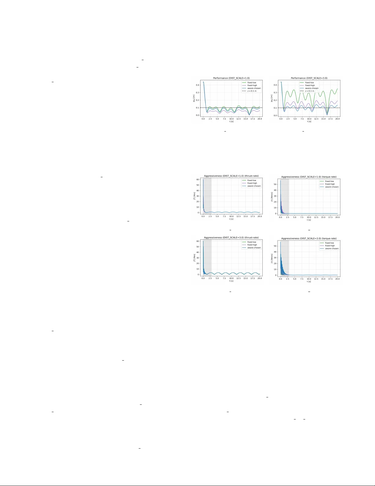
Aggr essiv eness-A war e Learning-based Contr ol of Quadr otor U A Vs with Safety Guarantees Leonardo Colombo, Thomas Beckers, Juan Giribet Abstract — This paper presents an aggr essiveness-awar e con- trol framework for quadrotor U A Vs that integrates learning- based oracles to mitigate the effects of unknown disturbances. Starting from a nominal tracking controller on SE(3) , unmod- eled generalized for ces and moments ar e estimated using a learning-based oracle and compensated in the control inputs. An aggressi veness-aware gain scheduling mechanism adapts the feedback gains based on probabilistic model-error bounds, en- abling reduced feedback-induced aggressiveness while guaran- teeing a prescribed practical exponential tracking performance. The proposed approach makes explicit the trade-off between model accuracy , r obustness, and control aggressi veness, and pro vides a principled way to exploit learning for safer and less aggressi ve quadrotor maneuvers. I . I N T RO D U C T I O N Quadrotor U A Vs are routinely required to track aggressive trajectories in cluttered and dynamic en vironments, where fast response and precise motion are ke y to safe operation. For this purpose, geometric control on S E (3) has emer ged as a principled approach that avoids singularities and yields L yapunov-based stability guarantees [1]. Aggressi ve flight and trajectory-generation pipelines further highlight the need for high-bandwidth tracking in practice [2]–[7]. In real flight, quadrotors are affected by complex aero- dynamic phenomena (drag, blade flapping, ground ef fect), rotor and frame asymmetries, and exogenous disturbances such as wind gusts. Such effects can be naturally repre- sented as unknown generalized forces and moments acting on the rigid-body dynamics. When these unknown terms are not accounted for , nominal geometric controllers may exhibit de graded tracking and steady-state errors. A widely used workaround is to increase feedback gains to recover performance. While effectiv e from a robustness standpoint, high-gain feedback typically increases feedback-induced ag- gr essiveness , manifesting as large variations and high rates L. Colombo is with Centre for Automation and Robotics (CSIC-UPM), Ctra. M300 Campo Real, Km 0,200, Arganda del Rey - 28500 Madrid, Spain. leonardo.colombo@csic.es Thomas Beckers is with the Department of Computer Science, V anderbilt Uni versity , Nashville, TN 37212, USA thomas.beckers@vanderbilt.edu Juan I. Giribet is with Universidad de San Andr ´ es (UdeSA) and CON- ICET , Argentina. jgiribet@conicet.gov.ar L. Colombo ackno wledge financial support from Grant PID2022- 137909NB-C21 funded by MCIN/AEI/ 10.13039/501100011033. The re- search leading to these results was supported in part by iRoboCity2030-CM, Rob ´ otica Inteligente para Ciudades Sostenibles (TEC-2024/TEC-62), funded by the Programas de Actividades I+D en T ecnolog ´ ıas en la Comunidad de Madrid. J. Giribet was supported by PICT -2019-2371 and PICT -2019- 0373 projects from Agencia Nacional de Investigaciones Cient ´ ıficas y T ec- nol ´ ogicas, and UBA CyT -0421BA project from the Univ ersidad de Buenos Aires (UB A), Argentina. in thrust and body torques, increased energy consump- tion, actuator saturation, and potentially unsafe behavior in proximity to humans or obstacles [8]–[10]. This motiv ates making explicit the trade-off between tracking performance and feedback-induced aggressiv eness, and dev eloping design tools that achiev e a prescribed tracking tolerance with the least aggressive feedback compatible with uncertainty . This paper proposes to reduce the reliance on high feed- back gains by augmenting geometric tracking control with a learned-based model of the unknown generalized disturbance forces and moments. The key idea is simple: better distur- bance compensation reduces model mismatch, which in turn allows smaller feedback gains while maintaining the same tracking specification. T o quantify this effect, we introduce a feedback-induced aggressi veness measure based on the sensitivity of the commanded generalized forces with respect to tracking-error variations. Inspired by stif fness-alteration viewpoints in feedback design [11], [12], we formalize aggressiv eness as a local input-sensitivity metric of the feedback term. W e then cast gain selection as an optimization problem: minimize feedback-induced aggressiv eness subject to a practical exponential tracking bound with a prescribed ultimate error lev el. T o enable implementable scheduling, we le verage high-probability model-error bounds provided by Gaussian-process (GP) oracles [13]–[16]. GP oracles for quadrotors UA Vs hav e been studied in [17]–[22]. Contribution: W e formulate an aggr essiveness-aware per- formance objectiv e for geometric quadrotor tracking control, capturing gain-induced sensitivity of thrust and torques via a local input-sensitivity metric. A learning-augmented con- troller is proposed that combines nominal geometric control with learning-based models of unknown generalized forces and moments, and characterize how residual model error affects the feedback gains required to meet a prescribed exponential tracking specification. W e pose gain tuning as minimizing feedback-induced aggressiv eness subject to a desired tracking-error bound, yielding a principled target for safe and accurate tracking in the presence of unmod- eled dynamics, and enabling an aggressiveness-a ware gain scheduling mechanism based on probabilistic error bounds. The remainder of the paper is structured as follows. Sec- tion II revie ws the quadrotor model, the nominal geometric tracking controller, and introduces the aggressi veness mea- sure. Section III presents the learning-augmented controller and the aggressi veness-aware stability and scheduling results. Section IV concludes the paper with numerical results, discussions, and highlights future research. I I . S Y S T E M M O D E L I N G A N D N O M I NA L C O N T R O L In this section, we introduce the modeling and control of quadrotor U A Vs, followed by the problem setting. In all the paper the mapping ( · ) ∧ : R 3 → so (3) and its in verse ( · ) ∨ denote the standard hat and vee isomorphisms between vectors in R 3 and elements of the Lie algebra so (3) of 3 × 3 ske w symmetric matrices. A. System class W e consider the model of a quadrotor U A V e volving on the special Euclidean group S E (3) as in [1]. The translational and rotational dynamics of the quadrotor are given by ˙ p = v , ˙ R = R ˆ ω m ˙ v = mg e 3 − T R e 3 + f trans ( x ) , J ˙ ω + ω × J ω = τ b + f rot ( x ) , (1) where p , v ∈ R 3 denote the position and velocity of the center of mass in the inertial frame, R ∈ S O (3) is the rotation matrix from body to inertial frame, ω ∈ R 3 is the angular velocity expressed in the body frame, m > 0 is the mass, J ∈ R 3 × 3 is the positiv e definite inertia matrix, g > 0 is the gravitational constant, and e 3 = [0 , 0 , 1] ⊤ . The control input is u =  T τ b  ∈ U ⊂ R 4 , where T ∈ R denotes the total thrust magnitude and τ b ∈ R 3 are the control torques expressed in the body frame. The admissible input set U collects physical constraints such as thrust and torque saturation limits. The full system state is x : = ( p , v , R, ω ) ∈ X := R 3 × R 3 × S O (3) × R 3 , (2) where ( p , R ) ∈ S E (3) are the configuration variables (position and attitude), and ( v , ω ) ∈ R 3 × R 3 are the corre- sponding linear and angular velocities. During the analysis we assume that the commanded inputs remain within the admissible set U on the compact set X c . The terms f trans : X → R 3 and f rot : X → R 3 represent unknown disturbances and unmodeled dynamics acting on the translational and rotational subsystems, respectiv ely (e.g., aerodynamic drag, wind gusts, and rotor asymmetries). W e also define the stacked generalized disturbance forces f ( x ) : =  f trans ( x ) f rot ( x )  ∈ R 6 . (3) Using local coordinates induced by the Lie algebra so (3) via the hat and vee isomorphisms, the system dynamics (1) can be represented in local Euclidean coordinates as a control-affine system of dimension 12 , ˙ x = f dyn ( x ) + G dyn ( x ) u + ¯ f ( x ) , (4) where x ∈ R 12 denotes the vector of local coordinates associated with ( p , v , R, ω ) ∈ X . Here, f dyn : R 12 → R 12 collects the known part of the quadrotor dynamics, G dyn : R 12 → R 12 × 4 is the kno wn input matrix. The term ¯ f ( x ) ∈ R 12 denotes the lifting of the generalized disturbance forces f ( x ) into the state-space coordinates, i.e., the contribution of f trans and f rot to the time deriv atives of ( v , ω ) in the local Euclidean representation. W e consider matched additiv e disturbances in the generalized coordinates, i.e., ¯ f ( x ) affects only the acceleration components in the local state representation. The input matrix G dyn ( x ) has constant rank 4 for all x ∈ X , reflecting the underactuated nature of the quadrotor system. W e are interested in tracking a sufficiently smooth refer- ence trajectory ev olving on X , ( p d ( t ) , ˙ p d ( t ) , R d ( t ) , ω d ( t )) ∈ X , (5) where p d ( t ) ∈ R 3 denotes the desired position, R d ( t ) ∈ S O (3) the desired attitude, and ˙ p d ( t ) and ω d ( t ) the corre- sponding desired linear and angular velocities. The associated tracking errors are defined as e p = p − p d , e v = v − ˙ p d , (6) e R = 1 2  R ⊤ d R − R ⊤ R d  ∨ , e ω = ω − R ⊤ R d ω d , (7) and collected in the stacked error vector e ( t ) =  e ⊤ p e ⊤ v e ⊤ R e ⊤ ω  ⊤ ∈ R 12 . (8) Remark 1: The nominal geometric tracking controller on S E (3) renders the tracking error almost-globally exponen- tially stable, except for a measure-zero set due to the topol- ogy of S O (3) [1]. In this work, we perform the analysis in local coordinates induced by the Lie algebra so (3) , which is sufficient for the study of learning-based disturbance com- pensation and feedback-induced aggressiveness. All results therefore hold locally around the desired trajectory , while inheriting the almost-global properties of the underlying geometric controller . ⋄ W e assume the existence of a nominal geometric tracking controller of the form u = h ff ( x , x d ) + h fb ( x ) H e , (9) where h ff : X × X → R 4 is a feedforward term deriv ed from the known dynamics f dyn and G dyn (e.g., as in geometric tracking control on S E (3) giv en in [1]), h fb : X → R 4 × 12 is a state-dependent feedback mapping, and H ∈ H ⊆ R 12 × 12 is a matrix of tunable feedback gains, typically chosen to be diagonal or block-diagonal and collecting the proportional and deriv ativ e gains associated with translational and rota- tional error components. The nominal control law (9) is designed under the assump- tion ¯ f ≡ 0 , i.e., neglecting the unknown disturbances and unmodeled dynamics. Under this assumption, the resulting nominal closed-loop state dynamics is ˙ x = f dyn ( x ) + G dyn ( x )  h ff ( x , x d ) + h fb ( x ) H e  . (10) When expressed in terms of the tracking error variables e = ( e p , e v , e R , e ω ) , this dynamics induce a closed-loop error system of the form ˙ e = ¯ f cl ( e , x d , H ) , (11) where ¯ f cl : R 12 × X × H → R 12 denotes the nominal closed- loop error vector field , obtained by substituting (10) into the time deriv ativ e of the error coordinates and expressing the result in local coordinates induced by the Lie algebra so (3) . W e restrict attention to a local chart induced by so (3) along the reference such that the error map Ψ( x , x d ) is smooth and its Jacobian w .r .t. x is bounded on the compact set X c containing the closed-loop trajectories. Assumption 1: For each H ∈ H , the nominal closed- loop error dynamics (i.e., ¯ f ≡ 0 ) admit a continuously differentiable L yapunov function V ( e ) = e ⊤ P ( H ) e with P ( H ) = P ( H ) ⊤ ≻ 0 and constants λ, λ, c 1 > 0 such that, for all e in a neighborhood E ⊂ R 12 , λ ∥ e ∥ 2 ≤ V ( e ) ≤ λ ∥ e ∥ 2 , ˙ V ( e ) ≤ − c 1 ∥ e ∥ 2 . (12) Remark 2: Assumption 1 is satisfied whenev er a geomet- ric tracking controller on S E (3) is av ailable for the known quadrotor dynamics that renders the tracking error locally exponentially stable (see [1] for controller construction). ⋄ Assumption 2: There exists a constant c 2 > 0 such that   ∇ e V ( e )   ≤ c 2 ∥ e ∥ , ∀ e ∈ E . (13) Remark 3: For the quadratic L yapunov function V ( e ) = e ⊤ P ( H ) e , a suitable choice is c 2 = 2 ∥ P ( H ) ∥ . ⋄ Remark 4: In practice, the “known” dynamics f dyn can be obtained from a simplified rigid-body model of the quadro- tor with nominal parameters, while complex aerodynamic effects, unmodeled dynamics, and parametric uncertainties are absorbed into the disturbance term ¯ f . This separation simplifies the design of the nominal controller (9). ⋄ Remark 5: Although the quadrotor is underactuated since G dyn ( x ) ∈ R 12 × 4 has rank 4 < 12 , the formulation on S E (3) together with a suitable choice of error coordinates ( e p , e v , e R , e ω ) allows the design of nominal tracking con- trollers that satisfy Assumption 1 directly on the configura- tion manifold. In particular , stability can be established with- out introducing additional virtual states or artificial control inputs, as the coupling between translational and rotational dynamics is handled intrinsically through the geometry of S E (3) and the attitude-dependent thrust direction. ⋄ The application of the nominal control law (9) to the actual dynamics (4) generally leads to a mismatch between the the- oretical performance guarantees and the observed behavior , due to the presence of the unknown disturbance term ¯ f . A naiv e remedy is to increase the feedback gains collected in H to reduce the tracking error . Howe ver , high feedback gains are often undesirable, as they result in aggressi ve attitude maneuvers, lar ge variations in thrust and body-frame torques, increased actuator stress, and potentially unsafe behavior . T o quantify this effect, we introduce a measure of feedback-induced aggr essiveness based on the sensitivity of the commanded control inputs with respect to v ariations in the tracking error . Since the generalized forces acting on the quadrotor are directly given by the control input u = ( T , τ b ) ∈ U , we focus on the feedback component of the control law (9). Inspired by the stiffness-alteration viewpoint in soft robotics [11], we define the feedback- induced aggressiveness as the mapping s : H × X → R ≥ 0 s ( H , x ) : =     ∂ ∂ e  h fb ( x ) H e      = ∥ h fb ( x ) H ∥ , (14) where the deriv ative is taken with respect to the tracking error e ∈ R 12 , treating the state x as a parameter , and the norm denotes an induced matrix norm. The quantity s ( H , x ) captures how strongly the commanded thrust and torques react to small deviations in the tracking error . Large values of s ( H , x ) correspond to aggressive feedback behavior , which can be problematic in proximity to obstacles or humans and may also excite unmodeled dynamics. B. Motivating Example T o illustrate the trade-off between feedback gains, tracking performance, and feedback-induced aggressiv eness in the quadrotor setting, we consider a simplified model of vertical motion around hover . This model is obtained from (1) by assuming small attitude deviations and focusing on the altitude dynamics. Let x 1 denote the altitude deviation from a desired constant height, and x 2 the corresponding vertical velocity . The dynamics are giv en by ˙ x 1 = x 2 , (15) ˙ x 2 = g − 1 m T | {z } f dyn ( x ) + f ( x ) | {z } unknown , (16) where m > 0 denotes the quadrotor mass, T is the total thrust command, and f ( x ) collects unknown effects such as ground effect, unmodeled aerodynamic drag, and external disturbances. The control objecti ve is to regulate the system to the equilibrium x d = 0 . A nominal controller for the vertical channel can be obtained by treating the thrust T as a virtual input and canceling the known gravity term, T = m  g + H e  = m  g + h 2 x 2 + h 1 x 1  , (17) where e = [ x 1 , x 2 ] ⊤ and H = [ h 1 , h 2 ] ∈ H = R 1 × 2 ≥ 0 collects the feedback gains. The resulting closed-loop dynamics is ˙ x 2 = − h 2 x 2 − h 1 x 1 + f ( x ) . (18) From a purely nominal control perspectiv e and neglecting the unknown term f ( x ) , increasing h 1 and h 2 improv es the rate of con vergence of the tracking error . In this case the feedback-induced aggressiveness becomes s ( H , x ) =     ∂ ∂ e  mH e      = m ∥ H ∥ 2 = m q h 2 1 + h 2 2 . (19) In the context of a quadrotor, increased aggressiveness manifests as large thrust variations around hover , leading to aggressiv e vertical accelerations, higher energy consumption, and potential actuator saturation. The required feedback gains can be reduced by incorpo- rating a learned model ˆ f of the unknown term f . The control law (17) is then modified to T = m  g + h 2 x 2 + h 1 x 1  − m ˆ f ( x ) , (20) which yields the closed-loop dynamics ˙ x 2 = − h 2 x 2 − h 1 x 1 +  f ( x ) − ˆ f ( x )  . (21) In the ideal case of perfect model matching, i.e., f = ˆ f , the equilibrium x d = 0 is asymptotically stable for any choice of h 1 , h 2 > 0 . More generally , improved model accuracy allows one to reduce the feedback gains required to achiev e a prescribed tracking performance, thereby lowering the feedback-induced aggressiv eness and avoiding overly aggressiv e thrust commands. Con versely , larger model errors necessitate higher feedback gains, resulting in more aggres- siv e and potentially less safe behavior . C. Pr oblem Setting The motiv ating example abov e illustrates the fundamen- tal trade-off between feedback gains, tracking performance, and feedback-induced aggressiv eness in a simplified verti- cal quadrotor model. An analogous trade-off arises for the full dynamics (4): increasing the feedback gains collected in H typically improves disturbance attenuation under the assumed continuous-time model and in the absence of input constraints, b ut simultaneously amplifies the sensitivity of the commanded thrust and body-frame torques with respect to tracking-error variations, as quantified by the measure (14). The objective of this article is to guarantee a prescribed tracking performance for the quadrotor while minimizing the feedback-induced aggressiveness associated with the control law (9). T o this end, we consider the system (4), where the unknown generalized disturbance forces are approximated by a learning-based oracle ˆ f : X → R 6 . The corresponding compensation is mapped into the physical input space via K dyn ( x ) and applied through the input matrix G dyn ( x ) . W e adopt the augmented control law u = h ff ( x , x d ) − K dyn ( x ) ˆ f ( x ) + h fb ( x ) H e , (22) where K dyn ( x ) ∈ R 4 × 6 is a known disturbance- compensation map that distributes the learned generalized forces and moments into the physical input space. T ypical choices for K dyn ( x ) include pseudoin verse- or least-squares- based mappings associated with G dyn ( x ) ; howe ver , perfect cancellation of ¯ f is not assumed. The functions h ff and h fb are as defined in (9). The resulting closed-loop tracking error dynamics depend on the (state-space) residual mismatch ∆( x ) = ¯ f ( x ) − G dyn ( x ) K dyn ( x ) ˆ f ( x ) and on the feedback gain matrix H . W e seek to select H ∈ H so that the tracking error remains uniformly bounded and conv erges practically exponentially to a neighborhood of the origin for all initial conditions in a (local) region of attraction. Specifically , for a prescribed ultimate tracking-error bound ε ∈ R > 0 , we require that for each feasible H ∈ H there exist constants γ 1 ( H ) , γ 2 ( H ) ∈ R > 0 such that the closed-loop tracking error satisfies: min H ∈H sup x ∈X c s ( H , x ) s.t. ∥ e ( t ) ∥ ≤ γ 1 e − γ 2 ( t − t 0 ) ∥ e ( t 0 ) ∥ + ε, ∀ t ≥ t 0 , (23) where X c ⊂ X is a compact set containing the relev ant closed-loop trajectories, s ( H , x ) is evaluated locally for e ≈ 0 , and the norm denotes any (conv ex) matrix norm (e.g., induced 2-norm or Frobenius norm). Remark 6: Since the feedback term is linear in e , we hav e s ( H, x ) = ∥ h fb ( x ) H ∥ , hence the objective H 7→ sup x ∈X c s ( H , x ) is con vex. If, in addition, the feasible set is nonempty and H is compact (e.g., by imposing ∥ H ∥ ≤ ¯ H ), then problem (23) admits at least one minimizer . ⋄ I I I . A G G R E S S I V E N E S S - A W A R E L E A R N I N G C O N T R O L W e address the problem in (23) with a learning-augmented control framework that balances model-based disturbance compensation and feedback g ains such that a prescribed tracking performance is achiev ed while reducing feedback- induced aggressiveness. The controller implements the augmented control law u = h ff ( x , x d ) − K dyn ( x ) ˆ f N ( x ) + h fb ( x ) H N e , (24) which augments the nominal geometric controller with a disturbance compensation term and an aggressiv eness-aware feedback gain matrix H N . Here, ˆ f N ( x ) ∈ R 6 denotes the oracle prediction of the generalized disturbance forces and moments, and K dyn ( x ) ∈ R 4 × 6 maps these estimates into the input space. When the oracle admits a uniform high- probability error bound on X c , smaller gains in H N can be sufficient to satisfy the prescribed practical tracking bound, thereby reducing the feedback-induced aggressiveness. Con- versely , larger model errors require increased feedback gains to maintain robustness. A. Oracle and Model Err or Bounds Recall that the unknown disturbances in (1) are captured by the generalized disturbance forces and moments f ( x ) =  f trans ( x ) f rot ( x )  ∈ R 6 . (25) W e consider an oracle that predicts f ( x ) for a giv en state x ∈ X . The oracle is trained from a dataset constructed from measured or estimated disturbance realizations obtained during closed-loop operation. Specifically , we define a time-varying dataset D ( t ) = { ( x { i } , y { i } ) } N ( t ) i =1 , (26) where N : R ≥ 0 → N denotes the (time-v arying) number of data points and y { i } ∈ R 6 is a data-driv en estimate of f ( x { i } ) . In practice, y can be obtained by subtracting the known model contributions from measured accelerations and applied inputs in (1). For notational simplicity , we consider piecewise-constant datasets over intervals t ∈ [ t N , t N +1 ) with 0 = t 0 < t 1 < t 2 < · · · and denote D N := D ( t ) on [ t N , t N +1 ) . The corresponding oracle at time t N is denoted by ˆ f N : X → R 6 , ˆ f N ( x ) = ˆ y | x , D N . (27) This formulation accommodates purely online learning, of- fline training with fixed datasets, as well as hybrid schemes. Between update times t N , the oracle and gains are held constant; the closed-loop system is thus piece wise-smooth with switching at { t N } . T o quantify oracle accuracy , we assume a high-probability bound on the model error ov er a compact set. Let X c ⊂ X be a compact set containing the relev ant closed-loop trajectories. Assumption 3: Consider an oracle with predictions ˆ f N ∈ C 0 based on D N . There exists a finite function ¯ ρ N : X c × (0 , 1] → R ≥ 0 such that, for any confidence level δ ∈ (0 , 1] , P n ∥ f ( x ) − ˆ f N ( x ) ∥ ≤ ¯ ρ N ( x , δ ) ∀ x ∈ X c o ≥ δ, (28) for any fixed N ∈ { 0 , 1 , . . . , N end } . Assumption 4: The number of dataset updates is finite: there exist N end ∈ N and T end ∈ R ≥ 0 such that D ( t ) = D N end for all t ≥ T end . Remark 7: The probability is taken w .r .t the measurement noise and the resulting oracle posterior (and, if applicable, the prior ov er f ). Assumption 3 ensures bounded model error in probability on X c , while Assumption 4 reflects practical limitations in memory and computational resources. ⋄ B. Gaussian Process as Oracle Gaussian process (GP) models provide a principled or- acle for nonlinear re gression with uncertainty quantifica- tion. W e adopt an independent-output GP construction to predict each component of f ( x ) ∈ R 6 . Let D N con- tain N D training pairs and define the input matrix X = [ x { 1 } , x { 2 } , . . . , x { N D } ] ∈ R 12 × N D and the output matrix Y ⊤ = [ ˜ y { 1 } , ˜ y { 2 } , . . . , ˜ y { N D } ] ∈ R 6 × N D , where ˜ y = y + η are noisy measurements corrupted by Gaussian noise η ∼ N (0 , σ 2 I 6 ) . For a query x ∗ , the GP posterior mean and variance for each output component i ∈ { 1 , . . . , 6 } are µ i ( x ∗ | D N ) = k ( x ∗ , X ) ⊤ K − 1 Y : ,i , (29) σ 2 i ( x ∗ | D N ) = k ( x ∗ , x ∗ ) − k ( x ∗ , X ) ⊤ K − 1 k ( x ∗ , X ) , where k is a positive definite kernel, k ( x ∗ , X ) = [ k ( x ∗ , x { 1 } ) , . . . , k ( x ∗ , x { N D } )] ⊤ , and K ∈ R N D × N D is the corresponding Gram matrix. Stacking the component-wise posteriors yields a Gaussian distribution with mean µ ( x ∗ | D N ) ∈ R 6 and diagonal cov ariance Σ( x ∗ | D N ) ∈ R 6 × 6 . Under standard regularity assumptions on the unknown function, this representation enables explicit high-probability error bounds. Assumption 5: The kernel k is chosen such that each component f i of f has a finite reproducing kernel Hilbert space norm on X c , i.e., ∥ f i ∥ k ≤ B i < ∞ for all i = 1 , . . . , 6 . Under Assumption 5 and standard GP concentration results, the prediction error admits a computable high- probability bound of the form (28), where ¯ ρ N ( x , δ ) can be expressed in terms of the posterior variance and information- gain quantities (see, e.g., [23]). C. Aggr essiveness-A ware Stability Guarantees Theor em 1: Consider the system (4) together with the learning-based control law (24). Suppose that Assumptions 1 and 2 hold, and that the oracle satisfies Assumption 3 on a compact set X c ⊂ X containing the closed-loop trajectories. Fix ε > 0 and δ ∈ (0 , 1] . Assume the oracle error bound satisfies sup x ∈X c ¯ ρ N ( x , δ ) ≤ c 1 2 c 2 ε, (30) where c 1 , c 2 correspond to the L yapunov inequalities for the chosen H N . Denote by E ⊂ R 12 a neighborhood of the origin in which the local error coordinates are valid and the nominal L yapunov conditions hold. Then, with probability at least δ , ev ery solution with x ( t ) ∈ X c and e ( t 0 ) ∈ E satisfies the practical exponential tracking bound ∥ e ( t ) ∥ ≤ γ 1 e − γ 2 ( t − t 0 ) ∥ e ( t 0 ) ∥ + ε, ∀ t ≥ t 0 , (31) for explicit constants γ 1 ( H N ) , γ 2 ( H N ) > 0 . Moreov er , assume that the gain-selection rule produces H N such that, on X c , ∥ H N ∥ ≤ κ 1 sup x ∈X c ¯ ρ N ( x , δ ) + κ 2 (32) for some constants κ 1 , κ 2 > 0 independent of N . Then the feedback-induced aggressiveness satisfies, for all x ∈ X c , s ( H N , x ) = ∥ h fb ( x ) H N ∥ ≤ α 1 ¯ ρ N ( x , δ ) + α 2 , (33) for constants α 1 , α 2 > 0 independent of N . In particu- lar , smaller model-error bounds ¯ ρ N enable lower feedback- induced aggressiveness while preserving (31). Pr oof: Under the control law (24), the closed-loop dynam- ics is ˙ x = f dyn ( x ) + G dyn ( x )  h ff ( x , x d ) + h fb ( x ) H N e  + ¯ f ( x ) − G dyn ( x ) K dyn ( x ) ˆ f N ( x ) . Let x d ( t ) be the reference and let e = Ψ( x , x d ) ∈ R 12 denote the stacked tracking error map ( e p , e v , e R , e ω ) . By construction Ψ( · , x d ) is smooth in local coordinates on the considered chart. Differentiating e = Ψ( x , x d ) yields ˙ e = ∂ Ψ ∂ x ( x , x d ) ˙ x + ∂ Ψ ∂ x d ( x , x d ) ˙ x d . Define the nominal error ¯ f cl ( e , x d , H N ) as the right-hand side obtained by setting ¯ f ≡ 0 and ˆ f N ≡ 0 , i.e., by replacing ˙ x above with f dyn ( x ) + G dyn ( x )  h ff ( x , x d ) + h fb ( x ) H N e  . Then the actual error dynamics can be written as ˙ e = ¯ f cl ( e , x d , H N ) + d N ( x ) , (34) where the perturbation term d N ( x ) is ∂ Ψ ∂ x ( x , x d )  ¯ f ( x ) − G dyn ( x ) K dyn ( x ) ˆ f N ( x )  . (35) Since ∂ Ψ ∂ x , G dyn , and K dyn are known smooth maps and x ( t ) ∈ X c by assumption, there exists c J > 0 such that   ∂ Ψ ∂ x ( x , x d )   ≤ c J for all x ∈ X c . Define ∆ N ( x ) : = ¯ f ( x ) − G dyn ( x ) K dyn ( x ) ˆ f N ( x ) ∈ R 12 . Then (35) can be compactly written as d N ( x ) = J ( x )∆ N ( x ) with J ( x ) : = ∂ Ψ ∂ x ( x , x d ) bounded on X c . T o connect the oracle bound in Assumption 3 to ∆ N , recall that ¯ f ( x ) is the lifting of the generalized distur- bance f ( x ) ∈ R 6 into local state coordinates. Thus, on X c there exists a bounded map B ( x ) such that ¯ f ( x ) = B ( x ) f ( x ) . Moreover , since G dyn and K dyn are continuous on the compact set X c , there exists c GK > 0 such that ∥ G dyn ( x ) K dyn ( x ) ∥ ≤ c GK for all x ∈ X c . Consequently , there exists a constant c ∆ > 0 such that, on X c , ∥ ∆ N ( x ) ∥ ≤ c ∆ ∥ f ( x ) − ˆ f N ( x ) ∥ . Therefore, on the event A δ = {∥ f ( x ) − ˆ f N ( x ) ∥ ≤ ¯ ρ N ( x , δ ) ∀ x ∈ X c } , which has probability at least δ by Assumption 3, ∥ ∆ N ( x ) ∥ ≤ c ∆ ¯ ρ N ( x , δ ) , ∀ x ∈ X c . Absorbing the constant factor c J c ∆ into ¯ ρ N (i.e., redefin- ing ¯ ρ N by a constant scaling), we may assume without loss of generality that (34) holds with d N ( x ) = ∆ N ( x ) and P { ∥ ∆ N ( x ) ∥ ≤ ¯ ρ N ( x , δ ) ∀ x ∈ X c } ≥ δ . Let V ( e ) = e ⊤ P ( H N ) e be the L yapunov function from Assumption 1. Along trajectories of (34), ˙ V ( e ) = ∇ e V ( e ) ⊤ ¯ f cl ( e , x d , H N ) + ∇ e V ( e ) ⊤ ∆ N ( x ) . By Assumption 1, ∇ e V ( e ) ⊤ ¯ f cl ( e , x d , H N ) ≤ − c 1 ∥ e ∥ 2 for all e ∈ E . Using Cauchy–Schwarz and Assumption 2, ˙ V ( e ) ≤ − c 1 ∥ e ∥ 2 + ∥∇ e V ( e ) ∥ ∥ ∆ N ( x ) ∥ ≤ − c 1 ∥ e ∥ 2 + c 2 ∥ e ∥ ∥ ∆ N ( x ) ∥ . On the ev ent A δ = {∥ ∆ N ( x ) ∥ ≤ ¯ ρ N ( x , δ ) ∀ x ∈ X c } , which has probability at least δ , we obtain ˙ V ( e ) ≤ − c 1 ∥ e ∥ 2 + c 2 ¯ ρ N ( x , δ ) ∥ e ∥ , ∀ x ∈ X c . (36) Assume (30). Then for all x ∈ X c , c 2 ¯ ρ N ( x , δ ) ≤ c 1 2 ε . Hence, whenever ∥ e ∥ ≥ ε , inequality (36) implies ˙ V ( e ) ≤ − c 1 ∥ e ∥ 2 + c 1 2 ε ∥ e ∥ ≤ − c 1 2 ∥ e ∥ 2 . Using V ( e ) ≥ λ ∥ e ∥ 2 from (12), we obtain for ∥ e ∥ ≥ ε , ˙ V ( e ) ≤ − c 1 2 λ V ( e ) . (37) Therefore, on any time interval during which ∥ e ( t ) ∥ ≥ ε , Gr ¨ onwall’ s inequality giv es V ( t ) ≤ V ( t 0 ) exp  − c 1 2 λ ( t − t 0 )  . Furthermore, on the boundary ∥ e ∥ = ε , (36) together with (30) yields ˙ V ( e ) ≤ − c 1 2 ε 2 < 0 , hence the set B ε = { e : ∥ e ∥ ≤ ε } is forward inv ariant on the e vent A δ . Thus, trajectories enter B ε in finite time and remain there. From (12), λ ∥ e ∥ 2 ≤ V ( e ) ≤ λ ∥ e ∥ 2 . Combining this with the decay estimate for V outside B ε yields ∥ e ( t ) ∥ ≤ s λ λ exp  − c 1 4 λ ( t − t 0 )  ∥ e ( t 0 ) ∥ until ∥ e ( t ) ∥ = ε. After the first hitting time of B ε , in v ariance implies ∥ e ( t ) ∥ ≤ ε . A standard stitching argument then yields (31) with γ 1 = q λ/λ and γ 2 = c 1 4 λ . This holds on A δ , hence with probability at least δ . By definition, s ( H N , x ) = ∥ h fb ( x ) H N ∥ ≤ ∥ h fb ( x ) ∥ ∥ H N ∥ . Since x ∈ X c and X c is compact, continuity of h fb implies sup x ∈X c ∥ h fb ( x ) ∥ < ∞ . Using (32), there exist constants α 1 , α 2 > 0 , independent of N , such that (33) holds. □ Cor ollary 1: Under the assumptions of Theorem 1, fix a confidence level δ ∈ (0 , 1] and assume that lim N →∞ sup x ∈X c ¯ ρ N ( x , δ ) = 0 . (38) Then, for any ε > 0 and any fixed H ∈ H , there exists N ε ∈ N such that for all N ≥ N ε the gain condition (30) holds (with c 1 , c 2 corresponding to that H ). Consequently , for each fixed N ≥ N ε , with probability at least δ , the tracking error satisfies ∥ e ( t ) ∥ ≤ γ 1 e − γ 2 ( t − t 0 ) ∥ e ( t 0 ) ∥ + ε, ∀ t ≥ t 0 , (39) with γ 1 = γ 1 ( H ) and γ 2 = γ 2 ( H ) , and the feedback-induced aggressiv eness satisfies lim sup N →∞ sup x ∈X c s ( H , x ) ≤ α 2 . (40) Pr oof: Fix ε > 0 and an y fixed H ∈ H . By (38), there exists N ε ∈ N such that for all N ≥ N ε , sup x ∈X c ¯ ρ N ( x , δ ) ≤ c 1 2 c 2 ε , where c 1 , c 2 correspond to the L ya- punov inequalities associated with the chosen fixed gain matrix H in Theorem 1. Hence the gain condition (30) of Theorem 1 holds for all N ≥ N ε , and therefore for each fixed N ≥ N ε the practical exponential bound (39) follows with probability at least δ . Moreov er , Theorem 1 implies that for each fixed N ≥ N ε (on the corresponding ev ent of probability at least δ ), for all x ∈ X c we have s ( H , x ) ≤ α 1 ¯ ρ N ( x , δ ) + α 2 . T aking sup x ∈X c on both sides and then lim sup N →∞ , and using (38), yields lim sup N →∞ sup x ∈X c s ( H , x ) ≤ α 1 lim N →∞ sup x ∈X c ¯ ρ N ( x , δ ) + α 2 = α 2 , which proves the claim. □ Pr oposition 1: Assume the setting of Theorem 1. Suppose that the residual perturbation in the err or dynamics can be decomposed as ∆ N ( x ) =  ∆ t,N ( x ) ∆ r,N ( x )  ∈ R 12 , ∆ t,N ( x ) , ∆ r,N ( x ) ∈ R 6 , with corresponding high-probability bounds ∥ ∆ t,N ( x ) ∥ ≤ ¯ ρ t,N ( x , δ ) , ∥ ∆ r,N ( x ) ∥ ≤ ¯ ρ r,N ( x , δ ) , ∀ x ∈ X c , holding on an event of probability at least δ . Assume further that there exist constants c t, 1 , c r, 1 > 0 such that, along the actual closed-loop trajectories, the L yapunov deriv ativ e satisfies ˙ V ( e ) ≤ − λ t ∥ e t ∥ 2 − λ r ∥ e r ∥ 2 + c t, 1 ∥ e t ∥ ∥ ∆ t,N ( x ) ∥ + c r, 1 ∥ e r ∥ ∥ ∆ r,N ( x ) ∥ , (41) where e t = [ e ⊤ p , e ⊤ v ] ⊤ ∈ R 6 , e r = [ e ⊤ R , e ⊤ ω ] ⊤ ∈ R 6 , and λ t , λ r > 0 depend monotonically on the translational gains ( K p,N , K v ,N ) and rotational gains ( K R,N , K ω ,N ) . Choose H N block-diagonal with translational and rota- tional blocks scheduled according to the gain-scheduling rule, and pick the coefficients c p , c v , c R , c ω such that λ t ≥ 2 √ 2 c t, 1 ε sup x ∈X c ¯ ρ t,N ( x , δ ) , (42) λ r ≥ 2 √ 2 c r, 1 ε sup x ∈X c ¯ ρ r,N ( x , δ ) . Then, on the e vent of probability at least δ , ˙ V ( e ) ≤ − 1 2 λ ∥ e ∥ 2 whenev er ∥ e ∥ ≥ ε, λ := min { λ t , λ r } , which implies practical exponential conv ergence of e ( t ) to an ε -neighborhood of the origin (cf. Theorem 1). Pr oof: Fix ε > 0 and consider the ev ent on which the bounds on ∆ t,N and ∆ r,N hold for all x ∈ X c . From (41) and the bounds, for any x ∈ X c , ˙ V ( e ) ≤ − λ t ∥ e t ∥ 2 − λ r ∥ e r ∥ 2 + c t, 1 ∥ e t ∥ ¯ ρ t,N ( x , δ ) + c r, 1 ∥ e r ∥ ¯ ρ r,N ( x , δ ) . T aking suprema o ver X c and defining ¯ ρ max t,N := sup x ∈X c ¯ ρ t,N ( x , δ ) and ¯ ρ max r,N := sup x ∈X c ¯ ρ r,N ( x , δ ) , ˙ V ( e ) ≤ − λ t ∥ e t ∥ 2 − λ r ∥ e r ∥ 2 + c t, 1 ¯ ρ max t,N ∥ e t ∥ + c r, 1 ¯ ρ max r,N ∥ e r ∥ . Now assume ∥ e ∥ ≥ ε , where ∥ e ∥ 2 = ∥ e t ∥ 2 + ∥ e r ∥ 2 . Since ∥ e t ∥ + ∥ e r ∥ ≤ √ 2 ∥ e ∥ , the scheduling conditions (42) imply c t, 1 ¯ ρ max t,N ∥ e t ∥ ≤ λ t ε 2 √ 2 ∥ e t ∥ , c r, 1 ¯ ρ max r,N ∥ e r ∥ ≤ λ r ε 2 √ 2 ∥ e r ∥ . Using ε ≤ ∥ e ∥ and ∥ e t ∥ + ∥ e r ∥ ≤ √ 2 ∥ e ∥ , we further obtain λ t ε 2 √ 2 ∥ e t ∥ + λ r ε 2 √ 2 ∥ e r ∥ ≤ λ 2 √ 2 ε  ∥ e t ∥ + ∥ e r ∥  ≤ λ 2 ∥ e ∥ 2 , λ := min { λ t , λ r } . Therefore, whenev er ∥ e ∥ ≥ ε , ˙ V ( e ) ≤ − λ t ∥ e t ∥ 2 − λ r ∥ e r ∥ 2 + λ 2 ∥ e ∥ 2 ≤ − λ ∥ e ∥ 2 + λ 2 ∥ e ∥ 2 = − λ 2 ∥ e ∥ 2 . Thus V ( e ) decreases outside the ε -ball in e . Standard com- parison arguments, together with the quadratic bounds on V from Assumption 1, imply practical exponential con ver gence to an ε -neighborhood of the origin. □ D. Implementation Procedur e W e conclude this section by summarizing the practical implementation steps of the proposed aggressiveness-a ware learning-augmented controller . 1) State estimation and err or computation. At each con- trol cycle, measure/estimate the current state x ( t ) (e.g., via IMU fusion and attitude/velocity estimation) and compute the tracking error e ( t ) w .r .t x d ( t ) . 2) Disturbance-label construction. Construct a data- driv en estimate y ( t ) ∈ R 6 of the generalized distur- bance f ( x ( t )) by rearranging the dynamics in (1), i.e., subtracting known model contributions from mea- sured/estimated accelerations and applied inputs. In practice, the required accelerations can be obtained from IMU-based estimates and/or filtered numerical differentiation of velocity and angular-rate estimates. Append the pair ( x ( t ) , ˜ y ( t )) to the dataset, where ˜ y ( t ) = y ( t ) + η ( t ) and η ( t ) models measurement noise (zero-mean sub-Gaussian noise, with Gaussian noise N (0 , σ 2 I 6 ) as a special case). 3) Oracle update (offline/online/hybrid). On each dataset update interval t ∈ [ t N , t N +1 ) , freeze the dataset as D N and train/update the oracle to obtain ˆ f N : X → R 6 (e.g., the GP posterior mean in Section III-B). 4) High-pr obability model-err or bound. Choose a com- pact set X c capturing the expected closed-loop operat- ing env elope (e.g., a tube around the reference trajec- tory) and compute a high-probability bound ¯ ρ N ( · , δ ) on X c such that, with probability at least δ , the oracle error is uniformly bounded on X c (cf. Assumption 3). For GP oracles, ¯ ρ N can be expressed in terms of posterior variances and information-gain quantities. 5) Aggr essiveness-awar e gain scheduling . Select feed- back gains H N ∈ H to satisfy the tracking specifica- tion while reducing feedback-induced aggressiv eness. In particular , enforce the sufficient condition (30) using conservati ve estimates/bounds for the L yapunov con- stants c 1 , c 2 in Assumptions 1–2. If separate transla- tional and rotational error bounds are available, sched- ule the corresponding blocks of H N (Proposition 1). 6) Learning-augmented contr ol input. Apply the learning- augmented control law (24). I V . N U M E R I C A L R E S U LT S W e ev aluate the proposed aggressiveness-a ware learning- augmented control framework via numerical simulations. The goal is to illustrate the trade-off between tracking per- formance and feedback-induced aggressi veness, and to show how an aggressiv eness-aw are gain selection can achiev e a prescribed tracking tolerance with reduced control variation. A. Simulation Setup The simulated quadrotor follows the model (1) with stan- dard small-scale U A V parameters (mass m = 1 kg and diagonal inertia). The vehicle tracks a smooth reference trajectory with nontrivial translational excitation in x – y and small altitude modulation, while maintaining constant yaw . W e report the position tracking error norm ∥ e p ( t ) ∥ and use the tolerance ε = 0 . 1 m as a practical tracking requirement ov er a simulation horizon of T = 20 s . T o emulate realistic model mismatch, we inject unknown external forces and moments that combine (i) drag-like terms, (ii) bounded lateral “wind” components, and (iii) persistent oscillatory disturbances in the vertical force and yaw moment channels, which require sustained control ac- tivity . The ov erall disturbance magnitude is scaled by a factor DIST SCALE ∈ { 1 , 3 } to represent moderate and sev ere mismatch scenarios. Throughout the reported runs, the commanded inputs remained within the set U . W e compare three gain-selection strategies: (i) fixed-low feedback gains (translation scaling trans scale = 1 . 0 ), (ii) fixed-high feedback gains ( trans scale = 1 . 8 ), and (iii) an aggr essiveness-aware selection that sweeps trans scale ∈ [1 . 0 , 2 . 5] and picks the smallest value that satisfies ∥ e p ( T ) ∥ ≤ ε when feasible (otherwise returning the best-performing value in the tested grid). In addition to the theoretical metric s ( H , x ) , aggressiv eness is quantified in simulation through observable input-v ariation metrics: the thrust-rate magnitude | ˙ T | and torque-rate norm ∥ ˙ τ ∥ . T o high- light transient effects, we compute RMS values separately on a transient window [0 , 3] s (shaded in gray in the plots) and on the steady windo w [3 , 20] s . B. P erformance–Aggr essiveness T rade-off T o emulate the gain-selection vie wpoint of (23) in a simulation setting, we implement a sweep-based scheduler: for a grid of v alues trans scale ∈ [1 . 0 , 2 . 5] , we simulate the closed loop and select the smallest gain that satisfies the practical tolerance ∥ e p ( T ) ∥ ≤ ε when feasible. In the theoretical de velopment, feasibility is certified via a model-error bound ¯ ρ N ( · , δ ) ; here we mimic this certification through the empirical sweep. a) Moderate disturbance ( DIST SCALE = 1 ).: Fig. 1 shows the performance–aggressiveness trade-off. Increasing feedback gains improves tracking: the final position error decreases from ∥ e p ( T ) ∥ = 0 . 116 m (fixed-lo w) to 0 . 060 m (fixed-high), while the peak error remains nearly unchanged (within numerical resolution, max t ∥ e p ( t ) ∥ ≈ 0 . 443 m ). This improv ement comes with increased transient aggressiv eness, as sho wn in Fig. 2: the transient RMS rises from | ˙ T | RMS , tr = 7 . 492 N / s and ∥ ˙ τ ∥ RMS , tr = 5 . 777 Nm / s (fixed-lo w) to 9 . 925 N / s and 8 . 201 Nm / s (fixed-high). In contrast, the steady-state torque-rate is nearly unchanged ( ∥ ˙ τ ∥ RMS , ss ≈ 0 . 059 Nm / s in both cases), indicating that the persistent oscillatory disturbances dominate the steady control modula- tion, whereas increased feedback mainly amplifies the tran- sient response. The aggressiveness-a ware scheduler selects trans scale = 1 . 2 as the smallest gain satisfying ε = 0 . 1 m , yielding ∥ e p ( T ) ∥ = 0 . 094 m while reducing transient aggressiv eness relativ e to fixed-high ( | ˙ T | RMS , tr = 8 . 121 N / s and ∥ ˙ τ ∥ RMS , tr = 6 . 416 Nm / s ). b) Sever e disturbance ( DIST SCALE = 3 ).: When the disturbance magnitude is tripled, fixed-low gains fail to meet the tolerance, ending at ∥ e p ( T ) ∥ = 0 . 351 m , while fixed-high gains improve tracking but still violate ε with ∥ e p ( T ) ∥ = 0 . 190 m . Within the tested grid, no gain value satisfies ε = 0 . 1 m ; the sweep therefore returns the best-performing tested gain (largest trans scale ), namely trans scale = 2 . 5 , resulting in ∥ e p ( T ) ∥ = 0 . 134 m . T ransient aggressiveness increases with gain magnitude (e.g., fixed-low versus fixed-high: | ˙ T | RMS , tr = 7 . 887 → 10 . 411 N / s and ∥ ˙ τ ∥ RMS , tr = 5 . 734 → 8 . 154 Nm / s ), and the largest gain further increases torque-rate transients ( ∥ ˙ τ ∥ RMS , tr = 10 . 886 Nm / s at trans scale = 2 . 5 ). Meanwhile, the steady torque-rate remains of comparable magnitude across strategies ( ∥ ˙ τ ∥ RMS , ss ≈ 0 . 177 Nm / s ). These results indicate that under sev ere mismatch, achieving strict tracking tolerances requires either improved distur- bance compensation or accepting higher aggressiv eness. (a) DIST SCALE = 1 (b) DIST SCALE = 3 Fig. 1: Tracking performance under fixed-lo w , fixed-high, and aggressiv eness-aware gain selection. The dashed line denotes the tolerance ε = 0 . 1 m . (a) | ˙ T | , DIST SCALE = 1 (b) ∥ ˙ τ ∥ , DIST SCALE = 1 (c) | ˙ T | , DIST SCALE = 3 (d) ∥ ˙ τ ∥ , DIST SCALE = 3 Fig. 2: Aggressi veness metrics under fixed-lo w , fixed-high, and aggressiveness-a ware gain selection. The shaded region marks the transient windo w [0 , 3] s used for transient RMS. C. GP-based disturbance compensation W e v alidate the theoretical results through numerical simulations under parametric mismatch and exogenous dis- turbances, and explicitly connect the observed feasibility– aggressiv eness trade-off to the probabilistic bounds. The disturbance oracle learns a 6 -dimensional generalized distur- bance (force + torque) using 6 independent GP regressors. Each regressor maps a 20 -dimensional feature vector z = [ p, v , q , ω , sin( · ) , cos( · ) , DIST SCALE ] to one component of [ f ⊤ , τ ⊤ d ] ⊤ ∈ R 6 . T raining data are collected from simula- tions at DIST SCALE ∈ { 1 , 3 } with target normalization by disturbance scale enabled ( normalize by dist=True ), yielding N D = 1162 samples with feature matrix Z ∈ R 1162 × 20 and target matrix Y ∈ R 1162 × 6 . The GP prior uses a squared-exponential (a.k.a. radial- basis-function, RBF) cov ariance with automatic relev ance determination (ARD), i.e., one characteristic length-scale per input coordinate, and an additive i.i.d. white-noise term. Concretely , for each output channel j ∈ { 1 , . . . , 6 } we fit an independent GP with kernel k j ( z , z ′ ) = σ 2 f ,j exp  − 1 2 20 X i =1 ( z i − z ′ i ) 2 ℓ 2 j,i  + σ 2 n,j δ z ,z ′ , where σ 2 f ,j is the signal variance (kernel amplitude), ℓ j,i are the ARD length-scales, and σ 2 n,j is the observ ation- noise variance. For the trained model, the learned ker - nel reported in the log (output 1) is k 1 ( z , z ′ ) = (0 . 928) 2 SE - ARD( z , z ′ ; ℓ ) + (10 − 6 ) δ z ,z ′ , with the op- timized ARD length-scales ℓ corresponding to the 20- dimensional feature vector used for GP regression. Large values (near the upper bound) indicate weak sensiti vity of the posterior mean to the associated feature, whereas smaller values identify the most informativ e coordinates for predicting the disturbance residual. T o ensure that GP-based compensation is applied only when the model is confident, the raw GP mean is fur - ther modulated by an uncertainty-based gate. Specifically , at each time step we compute a scalar uncertainty ρ ( t ) as the Euclidean norm of the predicted standard devia- tions across the six outputs, and apply a smooth sigmoid gate g ( ρ ) ∈ [0 , 1] (with reported steady-state average gate) so that compensation is suppressed when epistemic uncertainty is high. The gated compensation is addition- ally saturated and lo w-pass filtered to pre vent spurious high-frequency actuation. The GP-comp controller restores feasibility under severe mismatch: the learning-augmented loop achieves ∥ e p ( T ) ∥ = 0 . 028 m (well below ε = 0 . 10 m ) while keeping aggressi veness metrics comparable to the non-learning baselines (e.g., | ˙ T | RMS , tr = 8 . 066 N / s , ∥ ˙ τ ∥ RMS , tr = 6 . 077 Nm / s ; steady-state | ˙ T | RMS , ss = 2 . 251 N / s , ∥ ˙ τ ∥ RMS , ss = 0 . 175 Nm / s ). The steady-state gate mean remains high ( gate mean(ss) = 0 . 930 ), indicating consistent use of the learned compensation where the con- troller must overcome persistent oscillatory disturbances. Figure 3 reports tracking for three controllers: (i) a conservati ve baseline ( fixed-low ), (ii) a more aggres- siv e baseline ( fixed-high ), and (iii) the proposed GP- compensated controller with aggressiveness-a ware gain se- lection ( GP-comp (aware) ). In this regime, fixed-low fails to meet the tracking requirement ε = 0 . 10 m, ending at ∥ e p ( T ) ∥ = 0 . 351 m, and ev en fixed-high remains outside the tolerance with ∥ e p ( T ) ∥ = 0 . 190 m. In con- trast, GP compensation restores feasibility with ∥ e p ( T ) ∥ = 0 . 028 m while selecting the minimum translation gain scale that satisfies the tolerance in the offline sweep (here, trans scale = 1 . 0 ). Quantitative aggressi veness and effort metrics are reported in T able I. D. Online learning performance W e additionally report a representativ e online experiment to illustrate the behavior of the scheme when the disturbance oracle is refined during execution. The GP model is first Fig. 3: Numerical v alidation under sev ere mismatch ( DIST SCALE = 3 ): tracking performance for fixed-low , fixed-high , and GP-comp (aware) . The dashed line indicates the tracking tolerance ε = 0 . 10 m. Metric fixed-lo w fixed-high GP-comp (aware) ∥ e p ( T ) ∥ [m] 0.351 0.190 0.028 | ˙ T | RMS , tr [N/s] 7.887 10.411 8.066 ∥ ˙ τ ∥ RMS , tr [Nm/s] 5.734 8.154 6.077 | ˙ T | RMS , ss [N/s] 2.327 2.290 2.251 ∥ ˙ τ ∥ RMS , ss [Nm/s] 0.177 0.177 0.175 | T − mg | RMS , tr [N] 1.813 1.844 1.819 ∥ τ ∥ RMS , tr [Nm] 0.250 0.373 0.252 | T − mg | RMS , ss [N] 2.002 1.980 1.958 ∥ τ ∥ RMS , ss [Nm] 0.172 0.172 0.170 ∥ H ∥ F [–] 17.866 26.961 17.866 gate mean , ss [–] – – 0.930 ρ mean , ss [–] – – 0.069 T ABLE I: Numerical metrics for GP-based disturbance com- pensation with DIST SCALE = 3 . “tr” denotes t ∈ [0 , 3] s and “ss” t ∈ [3 , T ] . Ef fort metrics use T − mg and ∥ τ ∥ . trained offline and then updated online using streaming data and a gating/activ ation mechanism to pre vent unsafe corrections when uncertainty is high. W e compare: (i) fixed- low gains without learning (bas eline), (ii) of fline GP compen- sation using a GP prior trained offline, and (iii) of fline+online where a residual GP is updated online on top of the offline prior . In all cases, we report the position tracking error ∥ e p ( t ) ∥ and the aggressiv eness metrics | ˙ T | and ∥ ˙ τ ∥ , with transient and steady-state RMS computed on the same win- dows used throughout the paper , namely [0 , 3] s and [3 , 20] s. The offline dataset was collected ov er two disturbance lev els DIST SCALE ∈ { 1 , 3 } and yields Z ∈ R 1162 × 20 input features and Y ∈ R 1162 × 6 targets (3 force + 3 moment chan- nels). A six-output GP model was trained (independent GPs per output). T o limit the ef fect of potentially unreliable online updates, the residual GP correction is gated based on an uncertainty measure. In the reported run, the online residual GP acquired online points = 350 samples, and the gate statistics ov er steady-state were gate off mean(ss) = 0 . 911 and gate on mean(ss) = 0 . 982 , indicating that (i) the offline prior is trusted most of the time and (ii) the online Fig. 4: Online experiment, DIST SCALE = 3 . 0 . Position tracking error ∥ e p ( t ) ∥ for fixed-low (no GP), offline GP compensation, and offline+online residual GP . The dashed line denotes the tolerance ε = 0 . 10 m. residual is activ ated primarily when the uncertainty drops. The baseline fixed-low controller fails to satisfy the toler- ance under sev ere mismatch, ending at ∥ e p ( T ) ∥ = 0 . 351 m ( max t ∥ e p ( t ) ∥ = 0 . 442 m). In contrast, offline GP com- pensation satisfies the tolerance with ∥ e p ( T ) ∥ = 0 . 028 m, and adding the offline+online residual update yields a small further improvement to ∥ e p ( T ) ∥ = 0 . 025 m while preserving essentially the same aggressiv eness lev els. In particular, the transient RMS values remain comparable ( | ˙ T | RMS , tr = 8 . 066 N/s in both cases, and ∥ ˙ τ ∥ RMS , tr = 6 . 077 → 6 . 097 Nm/s), with steady-state rates essentially unchanged. These outcomes support the core message of the theory: improving the model/oracle reduces the residual perturba- tion entering the error dynamics, thereby enabling practi- cal exponential tracking with a prescribed tolerance while av oiding the need to increase feedback gains. In particular , for DIST SCALE = 3 . 0 the learning-augmented controller restores feasibility of the ε -tracking requirement that is violated by low-gain feedback alone. Future work will focus on hardware experiments on a real quadrotor platform to validate the proposed aggressiveness- aware learning controller under realistic aerodynamic effects, sensing noise, and onboard computational constraints. W e will in vestigate how to calibrate the uncertainty bounds and safety gates online from flight data so that prescribed tracking tolerances can be met with reduced control variation in prac- tice under real-world conditions. The simulations presented here are intentionally designed to isolate the performance– aggressiv eness mechanism; the experimental validation will include input saturation, discrete-time implementation, and state-estimation noise. R E F E R E N C E S [1] T . Lee, M. Leok, and N. H. McClamroch, “Geometric tracking control of a quadrotor uav on SE(3), ” in Proceedings of the 49th IEEE Confer ence on Decision and Contr ol (CDC) . Atlanta, GA, USA: IEEE, 2010, pp. 5420–5425. [2] D. Mellinger and V . Kumar, “Minimum snap trajectory generation and control for quadrotors, ” in Pr oceedings of the IEEE International Confer ence on Robotics and Automation (ICRA) . IEEE, 2011, pp. 2520–2525. [3] ——, “T rajectory generation and control for precise aggressi ve maneu- vers with quadrotors, ” The International Journal of Robotics Resear ch , vol. 31, no. 5, pp. 664–674, 2012. [4] L. Lu, A. Y unda, A. Carrio, and P . Campoy , “Robust autonomous flight in cluttered en vironment using a depth sensor , ” International Journal of Micr o Air V ehicles , vol. 12, p. 1756829320924528, 2020. [5] A. Rodriguez-Ramos, A. Alv arez-Fernandez, H. Ba vle, J. Rodriguez- V azquez, L. Lu, M. Fernandez-Cortizas, R. A. S. Fernandez, A. Rodelgo, C. Santos, M. Molina et al. , “ Autonomous aerial robot for high-speed search and intercept applications, ” F ield Robotics , vol. 2, pp. 1320–1350, 2022. [6] D. Falanga, E. Mueggler , M. Faessler , and D. Scaramuzza, “ Aggres- siv e quadrotor flight through narrow gaps with onboard sensing and computing using active vision, ” in 2017 IEEE international conference on r obotics and automation (ICRA) . IEEE, 2017, pp. 5774–5781. [7] B. T . Lopez and J. P . How , “ Aggressiv e 3-d collision avoidance for high-speed navigation. ” in ICRA , 2017, pp. 5759–5765. [8] R. Rashad, D. Bicego, J. Zult, S. Sanchez-Escalonilla, R. Jiao, A. Franchi, and S. Stramigioli, “Energy aware impedance control of a flying end-effector in the port-hamiltonian framew ork, ” IEEE T ransactions on Robotics , vol. 38, no. 6, 2022. [9] A. Franchi, R. Carli, D. Bicego, and M. Ryll, “Full-pose tracking control for aerial robotic systems with laterally bounded input force, ” IEEE T ransactions on Robotics , vol. 34, no. 2, pp. 534–541, 2018. [10] J. Breeden, K. Garg, and D. Panagou, “Control barrier functions in sampled-data systems, ” IEEE Contr ol Systems Letters , vol. 6, pp. 367– 372, 2022. [11] C. D. Santina, M. Bianchi, G. Grioli, F . Angelini, M. G. Catalano, M. Garabini, and A. Bicchi, “Controlling soft robots: Balancing feedback and feedforward elements, ” IEEE Robotics & Automation Magazine , vol. 24, no. 3, pp. 75–83, 2017. [12] T . Beckers, L. J. Colombo, M. Morari, and G. J. Pappas, “Learning- based balancing of model-based and feedback control for second-order mechanical systems, ” in 2022 IEEE 61st Conference on Decision and Contr ol (CDC) . IEEE, 2022, pp. 4667–4673. [13] T . Beckers, D. Kuli ´ c, and S. Hirche, “Stable gaussian process based tracking control of euler–lagrange systems, ” Automatica , vol. 103, pp. 390–397, 2019. [14] T . Beckers and L. Colombo, “Physics-informed learning for passivity- based tracking control, ” in 2025 IEEE 64th Conference on Decision and Contr ol (CDC) , 2025, pp. 2091–2096. [15] F . Berkenkamp and A. P . Schoellig, “Safe and robust learning control with gaussian processes, ” in Proceedings of the European Control Confer ence (ECC) , 2015. [16] F . Berkenkamp, A. P . Schoellig, and A. Krause, “Safe controller optimization for quadrotors with gaussian processes, ” in Pr oceedings of the IEEE International Conference on Robotics and Automation , 2016. [17] O. Y ago Nieto, A. Anahory Simoes, J. I. Giribet, and L. Colombo, “Dual-quaternion learning control for autonomous vehicle trajectory tracking with safety guarantees, ” arXiv pr eprint arXiv:2601.03097 , 2026. [18] O. Y ago Nieto and L. J. Colombo, “Safe learning-based control for an aerial robot with manipulator arms, ” IF AC-P apersOnLine , vol. 58, no. 6, pp. 36–41, 2024. [19] O. Y . Nieto, A. A. Simoes, J. I. Giribet, and L. J. Colombo, “Learning- based decentralized control with collision avoidance for multi-agent systems, ” IEEE T ransactions on Control of Network Systems , pp. 1–12, 2025. [20] T . Beckers, L. J. Colombo, and S. Hirche, “Safe trajectory tracking for underactuated vehicles with partially unknown dynamics, ” Journal of Geometric Mechanics , vol. 14, no. 4, pp. 491–505, 2022. [21] T . Beckers, L. J. Colombo, S. Hirche, and G. J. Pappas, “Online learning-based trajectory tracking for underactuated vehicles with uncertain dynamics, ” IEEE Contr ol Systems Letters , v ol. 6, pp. 2090– 2095, 2021. [22] L. J. Colombo and J. I. Giribet, “Learning-based fault-tolerant control for an hexarotor with model uncertainty , ” IEEE T ransactions on Contr ol Systems T echnology , vol. 32, no. 2, pp. 672–679, 2024. [23] N. Srinivas, A. Krause, S. M. Kakade, and M. Seeger, “Gaussian process optimization in the bandit setting: No regret and e xperimental design, ” in Pr oceedings of the 27th International Confer ence on Machine Learning (ICML) , 2010, pp. 1015–1022.