Comparative Evaluation of Machine Learning Models for Predicting Donor Kidney Discard

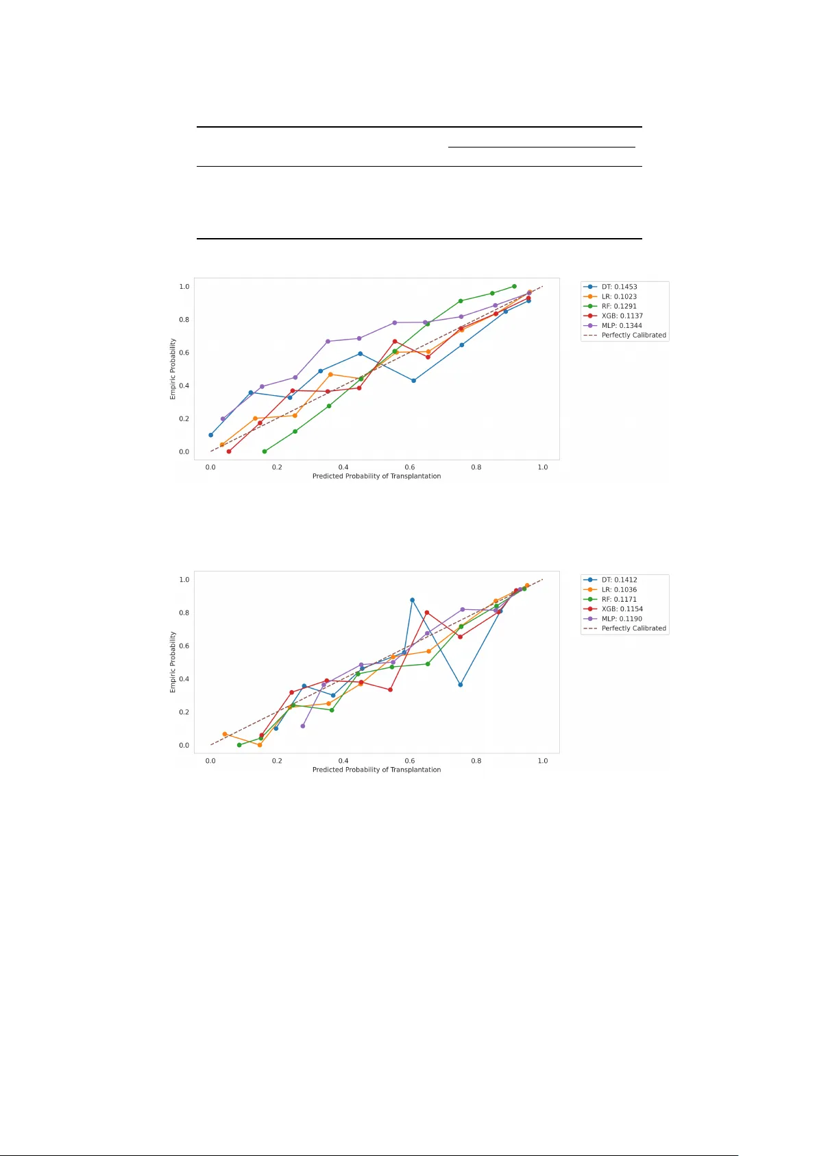
Comparativ e Ev aluation of Mac hine Learning Mo dels for Predicting Donor Kidney Discard P eer Sc hliephack e 1 † , Hannah Sc h ult 1 † , Leon Mizera 1 † , Judith W¨ urfel 1 † , Gun ter Grieser 2 , Axel Rahmel 3 , Carl-Ludwig Fisc her-F r¨ ohlic h 3 , An tje Jahn-Eimermac her 1* 1* Departmen t of Mathematics and Natural Sciences, Darmstadt Univ ersity of Applied Sciences, Sch¨ oﬀerstraße 3, Darmstadt, 64295, Hessen, Germany . 2 Departmen t of Computer Science, Darmstadt Univ ersity of Applied Sciences, Sch¨ oﬀerstraße 3, Darmstadt, 64295, Hessen, German y . 3 Deutsc he Stiftung Organ transplantation, Deutsc hherrnufer 52, F rankfurt, 60594, Hessen, German y . *Corresp onding author(s). E-mail(s): antje.jahn@h-da.de ; † These authors contributed equally to this work. Abstract A kidney transplan t can impro ve the life expectancy and qualit y of life of patien ts with end-stage renal failure. Even more patien ts could be help ed with a trans- plan t if the rate of kidneys that are discarded and not transplan ted could b e reduced. Machine learning (ML) can supp ort decision-making in this context b y early identiﬁcation of donor organs at high risk of discard, for instance to enable timely interv entions to improv e organ utilization such as rescue allo ca- tion. Although v arious ML mo dels ha ve been applied, their results are diﬃcult to compare due to heterogenous datasets and diﬀerences in feature engineer- ing and ev aluation strategies. This study aims to provide a systematic and repro ducible comparison of ML mo dels for donor kidney discard prediction. W e trained ﬁv e commonly used ML models: Logistic Regression, Decision T ree, Random F orest, Gradient Bo osting, and Deep Learning along with an ensem- ble mo del on data from 4,080 deceased donors (death determined b y neurologic criteria) in Germany . A uniﬁed b enc hmarking framework was implemen ted, including standardized feature engineering and selection, and Bay esian h yperpa- rameter optimization. Model performance w as assessed for discrimination (MCC, 1 A UC, F1), calibration (Brier score), and explainability (SHAP). The ensem- ble achiev ed the highest discrimination p erformance (MCC=0.76, AUC=0.87, F1=0.90), while individual models suc h as Logistic Regression, Random F orest, and Deep Learning p erformed comparably and better than Decision T rees. Platt scaling improv ed calibration for tree-and neural netw ork-based mo dels. SHAP consisten tly iden tiﬁed donor age and renal markers as dominan t predictors across mo dels, reﬂecting clinical plausibility . This study demonstrates that consisten t data prepro cessing, feature selection, and ev aluation can b e more decisive for predictiv e success than the c hoice of the ML algorithm. Keyw ords: Organ T ransplan tation, Donor Kidney Discard, Machine Learning, Calibration, Explainable AI, F eature Selection 1 In tro duction The global shortage of donor organs remains a signiﬁcan t challenge in modern medicine. While the demand for transplants contin ues to rise, organ donations ﬂuc- tuate [ 1 ] and often fall short of clinical needs. At the same time, the qualit y of donor organs has declined, with increasing donor age and a reduced num ber of usable organs p er donor [ 2 ]. These circumstances make allo cation and acceptance decisions b oth highly complex and time-critical as preserv ation limits and ischemic-time related risks imp ose strict time constraints. As a consequence a substantial prop ortion of retrieved donor kidneys is ultimately discarded. Therefore, a research question of particular rel- ev ance in this context is the early iden tiﬁcation of donor organs at high risk of b eing discarded, for instance to enable interv entions to increase organ utilization such as timely rescue allo cation eﬀorts or applying mac hine p erfusion to improv e organ quality . Mac hine learning (ML) mo dels can supp ort clinical decision-making by making use of the large v olumes of av ailable data, including biopsy rep orts, laboratory v alues, and free-text clinical records. Consequently , v arious ML mo dels hav e b een applied in the con text of organ transplantation, often with promising results [ 3 – 8 ]. Thereby , kidney transplan tation represents a frequently studied area due to the relatively large num ber of a v ailable cases. Commonly used ML mo dels include Decision T rees (DT) and Regres- sion Mo dels as w ell as more ﬂexible metho ds such as Random F orests (RF), Gradient Bo osting, and artiﬁcial neural netw orks, which are generally less in terpretable but ma y oﬀer higher predictiv e p erformance. These mo dels also hav e b een applied to the sp eciﬁc task of predicting kidney discard risk, yielding heterogeneous results: Logistic regression (LR) remains one of the most commonly used approaches in this context, iden tifying key predictors asso ciated with organ discard, suc h as biopsy ﬁndings and high Kidney Donor Proﬁle Index scores [ 5 , 9 – 13 ]. Some studies rep ort impro ved pre- dictiv e p erformance when using more adv anced ML mo dels, such as gradien t b oosting or RF [ 7 , 14 ]. Other studies ha v e found ML approac hes to perform similarly to LR [ 15 ]. Ho wev er, these studies are diﬃcult to compare directly , as the underlying datasets v ary substan tially . F or example, one study analyzed a large national dataset with several h undred predictors, whereas another relied on single-center data with a muc h smaller 2 sample size and a limited set of predictors. F urthermore, the role of feature selec- tion [ 16 ] is often o v erlo ok ed, p oten tially fav oring models with built-in feature selection mec hanisms suc h as RF. This mak es it diﬃcult to draw systematic conclusions ab out whic h mo dels are most suitable for predicting kidney discard risk and thus supp ort- ing clinical decision-making in organ transplan tation. The aim of this study was to address this gap b y systematically comparing diﬀerent ML approaches for predicting kidney discard risk, using a consistent prepro cessing and transformation pip eline on a shared dataset of kidney transplantation candidates. This work mak es tw o main contributions. First, multiple state-of-the-art ML mo d- els are systematically ev aluated with adv anced techniques such as mo del calibration and Bay esian h yp erparameter optimization applied to ensure an ob jectiv e comparison. Second, not only prediction p erformance but also mo del explainabilit y is compared through the use of SHAP , which enables the iden tiﬁcation of key predictors and supp orts clinical in terpretability . Although the proprietary data used in this study cannot b e shared b ecause of con- ﬁden tiality restrictions, w e pro vide comprehensive access to all accompanying scripts for data pro cessing, feature engineering and selection, mo del optimization, training, ev aluation, calibration, and visualization to promote transparency and reproducibility . The structure of this pap er is as follows. Section 2 describ es the data, the ML mo dels, and feature engineering strategies, follow ed b y an outline of the mo del ev alu- ation methodology . Section 3 presen ts the results of the mo del comparison, including discrimination p erformance, mo del calibration and explainability . Finally , Section 4 concludes the pap er and highlights directions for future work. 2 Metho ds 2.1 Data Data on all kidneys oﬀered for transplan tation from deceased adult donors in Germany b et w een April 2020 and August 2024 w ere used. The dataset, pro vided b y the German Organ Pro curemen t Organization (DSO), includes information from n = 4080 adult donors (all deaths determined by neurological criteria). Only donor-related character- istics are considered in predicting whether a kidney would discarded, while recipient c haracteristics are inten tionally excluded. This approach enables the identiﬁcation of donor kidneys at high risk of discard based solely on information av ailable at the time of the organ oﬀer, prior to allo cation to a sp eciﬁc recipient. Donor data w ere provided b y the German Organ Pro curemen t Organization (DSO) as an indep enden t researc h database for secondary analysis. All iden tiﬁers w ere remo ved, and only anon ymized data are included. The dataset includes those data that the DSO is legally required to provide to the national transplan tation registry under national transplan tation la w (TPG). The secondary analysis of these anon ymized data w as conducted in compliance with the transplan tation la w. An organ is deﬁned as discarded if it w as oﬀered for transplan tation but ultimately not transplan ted for any reason. Discard is considered at the donor lev el rather than the organ level to ensure indep endent observ ations and circumv en t intra-individual correlations. In most cases (3,716 out of 4,080), b oth kidneys from a donor were either 3 transplan ted or discarded, making a donor-level classiﬁcation straightforw ard. In 364 cases, only one kidney was transplanted while the other was discarded. These cases are classiﬁed as “transplanted” at the donor level. In summ ary , 929 (22 . 8%) of all donors are classiﬁed as discarded and 3151 (77 . 2%) of all donors are classiﬁed as trans- plan ted (i.e. not discarded). Note, that for a small num b er of donors, inconsistencies in kidney transplantation status w ere observed. Due to data anonymization, these inconsistencies could not b e resolv ed, and the data were therefore analyzed as reporte. Donors providing m ultiple organs are not excluded as organ combinations do not in teract with kidney discard. They may inﬂuence p ost-transplan t function, which w as ho wev er not the fo cus of this study . The data comprises results from examinations of v arious b ody parts, information ab out any medication that had b een prescrib ed, lab oratory measurements from the domains of virology , pathology and microbiology as well as details on hospital stays and medical diagnoses including ICD-10 co des (In ternational statistical classiﬁcation of diseases and related health problems) [ 17 ]. In summary , p=1128 v ariables are av ail- able and were further pro cessed in the feature engineering step (see section 2.2 ). A comprehensiv e description of the study cohort across all these v ariables is not feasible. Therefore, we extract the features that will later turn out to b e most imp ortan t for prediction and summarize them in T able 1 . The dataset w as split based on donor id allo cating 80% of donor ids to the training set and 20% to the test set to ensure indep endence b et ween training and ev aluation data. F eature Engineering was executed on b oth sets separately with thresholds cal- culated on only the training set and applied on the test set. Additionally , a ﬁxed 10% subset of the training data was reserv ed as a dedicated v alidation set for ﬁnal mo del training and calibration, ensuring strict separation from the held-out test set used for ﬁnal ev aluation. 2.2 F eature Engineering In this section, we describe feature transformations including time series pro cessing, redundancy reduction, enco ding of categorical v ariables and imputation of missing v alues. Some additional transformations of speciﬁc features are describ ed in Appendix B . V ariables were selected, extracted and engineered without prior ﬁltering b y medical advisors to av oid selection bias. Only in cases of uncertaint y primary inv estigators consulted medical experts to ensure appropriate data standardization (e.g. donor urine output adjusted to b o dy weigh t of donor and standard time interv al as ml /k g/h ). Secondary v alidation was p erformed by medical advisors to ensure that the data reﬂect real w orld scenarios in deceased organ donation pro cedures. 2.2.1 F eature Extraction from Time Series Man y of the lab oratory measurements come in the form of time series. 49 v ariables were iden tiﬁed as time series. An additional 40 v ariables were not considered time series, as more than 50% of donors had only a single recorded v alue for these v ariables. F or these w e chose either the most recen t or the ﬁrst recorded v alue. W e categorized the time 4 T able 1 Descriptive statistics of the most inﬂuential features as rep orted in Figure 6 . Individual dummy v ariables from one-hot encoding were excluded, as they do not capture the full information of the original categorical v ariable. F eature All donors T ransplanted Discarded N = 4080 N = 3151 N = 929 V ariables originally reported: Age (years), median [IQR] 58.0 [46.0, 69.0] 56.0 [44.0, 66.0] 68.0 [56.0, 78.0] Diuresis ( kg / 24 h/kg (bo dy weigh t)), median [IQR] 36.88 [24.21, 53.33] 38.55 [26.52, 57.1] 30.59 [15.06, 42.86] Heparinoids administered, n (%) 3873 (94.9) 3128 (99.3) 745 (80.2) V ariables extracted from time series: eGFR MDRD ( ml/min/ 1 . 73 m 2 ), median [IQR] - minimum 69.69 [44.92, 95.12] 76.45 [53.84, 100.42] 39.48 [19.81, 66.8] Creatinine ( g /l ), median [IQR] - Minimum 0.78 [0.6, 1.0] 0.72 [0.58, 0.9] 1.02 [0.77, 1.5] - Maximum 97.2 [74.22, 141.61] 88.4 [70.7, 123.8] 154.7 [97.2, 291.7] - Intercept 81.58 [61.93, 116.02] 75.92 [59.47, 101.44] 118.88 [84.0, 197.31] - Last 79.6 [61.9, 114.9] 75.1 [59.2, 99.0] 118.5 [79.6, 193.6] - Standard deviation 11.22 [5.79, 22.55] 10.3 [5.36, 18.8] 19.59 [7.47, 59.77] Nitrite, median [IQR] - Count 1.0 [1.0, 1.33] 1.0 [1.0, 1.32] 1.0 [1.0, 1.33] Urea ( mmol/l ), median [IQR] - Minimum 4.3 [3.0, 5.9] 4.0 [2.8, 5.3] 5.9 [4.2, 8.0] - Maximum 7.0 [5.0, 10.0] 6.3 [4.7, 9.0] 9.9 [6.8, 16.3] Bloo d gases FIO2 (1 / 1), median [IQR] - First 0.51 [0.4, 0.7] 0.51 [0.4, 0.79] 0.54 [0.4, 0.68] Bloo d gases pH, median [IQR] - Count 2.0 [1.0, 3.0] 2.0 [1.0, 3.0] 2.0 [1.0, 2.34] Potassium ( mmol/l ), median [IQR] - Maximum 4.5 [4.2, 4.9] 4.5 [4.2, 4.9] 4.7 [4.4, 5.2] INR (1 / 1), median [IQR] - First 1.1 [1.01, 1.25] 1.1 [1.0, 1.23] 1.14 [1.05, 1.3] Nitrite negative, n (%) - First 3499 (85.8) 2830 (89.8) 669 (72.0) Glucose negative, n (%) - First 2928 (71.8) 2392 (75.9) 536 (57.7) Protein qualitative negative, n (%) - First 2069 (50.7) 1772 (56.2) 297 (32.0) Protein qualitative negative, n (%) - First 2082 (51.0) 1790 (56.8) 292 (31.4) series v ariables into the follo wing subtypes to maximize the extracted information for eac h v ariable: • T yp e 1: Time series v ariables with categorical v alues, that indicate a p ositiv e or negativ e outcome only . • T yp e 2: Time series v ariables with numerical v alues and a mean n umber of observ ations p er donor low er than tw o. • T yp e 3: Time series v ariables with numerical v alues and a mean n umber of observ ations p er donor of tw o or more. F or eac h time series v ariable, w e extracted the follo wing features for ev ery donor: the ﬁrst recorded v alue, the last recorded v alue, the num b er of entries, and the time span b et w een the ﬁrst and last en try (measured in hours). F or time series v ariables with numerical v alues (type 2 and 3) we also extracted the standard deviation, minimum, and maxim um v alues. 5 F or time series v ariables of type 3, we further extracted features describing the linear trend ov er time: A linear regression per donor was p erformed mo deling the v alue of the v ariable (dep endent v ariable) ov er time measured in hours since the ﬁrst en try (indep enden t v ariable). Thus, the linear regression mo del for every donor d is: y d,i = β d, 0 + β d, 1 · t i + ε d,i (1) where y d,i denotes the v alue of the v ariable at the time p oin t t i . The estimated co eﬃcien ts ˆ β d, 0 and ˆ β d, 1 w ere used as additional features. Previous studies use the last recorded v alue [ 18 ] or the minimum v alue [ 18 , 19 ]. Our additionally extracted features may capture changes ov er time: The num b er of en tries ma y indicate that v ariable v alues for a donor ha ve changed ov er time. Similarly , the time span b etw een the ﬁrst and last entry can also reﬂect temporal dynamics in the donor’s condition. The standard deviation also provides insigh ts into the level of v ariabilit y . The estimated linear regression co eﬃcien ts include information on whether the v alues generally increased or decreased o ver time and to what extent. In summary , a total of 364 features were extracted from the time series data. 2.2.2 F eature Extraction from Donor Medication Data In the raw data there are 1772 unique medication names. These are structured such that the ﬁrst word describ es the medication and the remaining ones give additional information suc h as dosage. Considering only the ﬁrst w ord of eac h medication en try reduced the num b er of medication names to 1103. Afterwards, the 40 most frequen t medication names w ere selected for the ﬁnal feature set. This selection captures appro ximately 80% of all medication administrations in the dataset. They were turned in to binary features indicating, whether a donor had tak en the medication or not. 2.2.3 Categorical V ariable Enco ding W e used One-Hot enco ding for categorical v ariables with more than tw o v alues. Thereb y , for v ariables containing ICD-10 codes , w e replaced co des with a relative frequency of less than 1% of donors in the training set b y missing v alues. 2.2.4 Missing V alue Imputation Appro ximately 14% of the v alues in our data are missing with 628 of the v ariables ha ving incomplete data. These w ere imputed in the sam e wa y in training and test set unless stated otherwise as follo ws: • 250 v ariables could be imputed using logical dep endencies follo wing exp ert advice. These include v ariables on certain diagnoses where a missing v alue can be in terpreted as a negative v alue (i.e. no diagnosis present). • F or some categorical v ariables missing v alues were kept and considered a separate category . These are v ariables where a missing v alue is considered to p oten tially inﬂuence the decision ab out discard (e.g. ’urine glucose’). • F or t wo v ariables (’CPR duration’ and ’ecmo’) free text v ariables provided additional information and were used for imputation. 6 • 30 contin uous v ariables describing physiological parameters were imputed with ran- dom samples from a normal distribution with mean and standard deviation of each v ariable, retaining only v alues from within the central 95% range of this distribution. The distribution was calculated separately for training and test set. • F or 20 v ariables with a high p ercen tage of missing v alues ( > 70%) in the training set the speciﬁc v alues w ere dropp ed and the v ariables dic hotomized into ”missing” and ”not missing”. In these cases imputation based on sparse data was considered unreliable and therefore not performed. • The remaining 328 v ariables with missing v alues in the training set were imputed with an iterative imputing algorithm [ 20 ] using ridge regression to predict the miss- ing v alues for both training and test set. If there were v ariables with missing v alues in the test set that had no missing v alues in the training set, these w ere ﬁlled with the mean of that v ariable. This metho d was c hosen to account for complex relationships betw een v ariables. Finally , we ev aluated the result of this imputation strategy using a Histogram- based Gradien t Bo osting Classiﬁcation T ree. The HistGradientBoostingClassiﬁer has an in trinsic metho d for imputing missing v alues [ 21 ] and results relying on this method can b e compared to results with prior imputation using our imputation strategy . W e trained a HistGradientBoostingClassiﬁer on the training set of b oth the ﬁnal imputed feature set as w ell as the original version without imputation using a grid searc h and ﬁve-fold cross-v alidation. P erformance on the test set (F1 sc ore and MCC) was compared. The scores relying on our imputation strategy were sup erior to those of the intrinsic strategy of the HistGradientBoostingClassiﬁer, indicating a successful imputation strategy . 2.3 Mo deling Approach The following section outlines our modeling approach, including the ML algorithms, feature selection tec hniques, and h yp erparameter optimization metho ds applied to the kidney transplan tation dataset. 2.3.1 Mac hine Learning Algorithms The follo wing ML algorithms are trained to predict the probabilities of donor organs b eing either discarded or transplanted. Decision T rees Decision T rees (DTs) [ 22 ] are sup ervised learning mo dels used for classiﬁcation and regression tasks. They split data recursiv ely in to subsets based on feature thresholds, forming a tree-lik e structure where eac h internal no de represen ts a decision and eac h leaf no de provides a ﬁnal prediction. DTs are kno wn for their interpretabilit y , as each split is based on simple rules deriv ed from an impurit y measure such as the Gini impurit y , but are prone to o verﬁtting [ 22 ], esp ecially when the tree is deep. 7 Logistic Regression Logistic Regression (LR) [ 23 ] is a ML algorithm from the linear family , commonly used for binary classiﬁcation tasks. LR mo dels the probability of an outcome by applying a sigmoid function (logistic) to a linear combination of input features. The regression mo del usually uses the least squares metho d to ﬁnd the parameters for each fea- ture whic h minimize the sum of squared errors regarding the target v ariable [ 23 ]. An additional adv antage is its in terpretability , since feature imp ortance can b e directly inferred from the mo del co eﬃcien ts. Random F orest Random F orest (RF) [ 24 ] is an ensem ble learning metho d that builds multiple DTs and com bines their outputs to improv e predictive accuracy and decrease ov erﬁtting. The forest mo del uses the bagging metho d by training each tree on a random subset of the data and features resulting in reduced ov erﬁtting compared to individual DTs. An additional adv an tage is the p ossibilit y to derive aggregated feature imp ortance measures across all trees, whic h enhances in terpretabilit y . eXtreme Gradient Bo osting Extreme Gradient Bo osting (XGB) [ 25 ] is an ensemble learning algorithm based on gradien t b o osting [ 26 ], suitable for classiﬁcation and regression tasks. The mo del builds DTs sequentially , where eac h new tree corrects the errors of the previous ones, optimiz- ing p erformance through gradien t descent. XGB p erforms esp ecially w ell on structured data [ 27 ] and can ev en outp erform deep learning algorithms [ 28 ]. An additional adv an- tage is the av ailability of feature importance measures which pro vide interpretabilit y despite the mo del’s complexit y . Multila y er Perceptron Multila yer Perceptron (MLP) (also known as Deep Learning) [ 29 ] is an artiﬁcial neu- ral netw ork used for b oth classiﬁcation and regression tasks. It consists of multiple la yers of in terconnected neurons, including an input la yer, one or more hidden la y ers and an output lay er, where each neuron applies a weigh ted sum of inputs follow ed b y a nonlinear activ ation function. MLPs are capable of capturing complex, nonlin- ear relationships but require careful tuning of hyperparameters and large datasets to generalize well. Although they are more commonly applied to unstructured data such as images or text, MLPs can also b e used on structured tabular data. Ensem ble An ensemble mo del, referred to as the data ensemble mo del (DE), was implemented to combine the predictions of several pretrained classiﬁers. In this study the DE in te- grates the outputs of LR, XGB, RF and MLP . Each mo del pro duces a probability for b oth classes and the ensemble aggregates these outputs by computing the mean of the predicted probabilities across mo dels. The ﬁnal classiﬁcation result is deter- mined b y selecting the class with the highest av eraged probabilit y . Decision T rees were 8 excluded from the ensem ble due to their comparativ ely low er p erformance, as will b e demonstrated in later sections. 2.3.2 F eature Selection T o address the high dimensionality of our dataset, we apply a feature selection approac h to identify the most promising subset of features. This reduces redundancy , impro ves mo del interpretabilit y , and prev ents o verﬁtting by fo cusing on the v ariables most relev an t to prediction [ 16 ]. Because diﬀerent machine learning mo dels capture relationships in distinct wa ys, we p erform the feature selection separately for each mo del but alwa ys with the same metho d. This ensures that each algorithm op erates on a feature set tailored to its sp eciﬁc inductiv e biases and complexity . T o capture nonlinear and multiv ariate interactions b etw een features, w e employ an optimization metho d based on genetic algorithms [ 30 ] with their ability to navigate large search spaces [ 31 ]. This approach can uncov er complex relationships that simpler univ ariate ﬁlters (e.g., correlation or c hi-square tests) ma y miss [ 32 , 33 ]. The general approach is applied separately for each ML mo del as depicted in Figure 1 and describ ed in the following. 9 Fig. 1 Schema of the feature selection process. Starting from the full feature space, m ultiple candi- date feature subsets are created and ev aluated b y training and v alidating a sup ervised model. Each subset is assigned a loss v alue based on its predictive p erformance, and the subset with the smallest loss is selected as the ﬁnal feature subset. W e use the Nondominated Sorting Genetic Algorithm I I (NSGA-I I) [ 34 ] for single-ob jective feature selection optimization, as it nativly handles binary and cate- gorical parameters, unlik e other evolutionary strategies [ 35 ]. W e use the optuna [ 36 ] implemen tation fothe NSGA-II algorithm. 1. First, a p opulation of 50 randomly selected feature subsets are selected as candi- dates. F eature sets here are represen ted as b oolean v ector of length ∼ 1100 (n um b er 10 of features in the feature set) where each element represents a feature and is set to either one or zero depending whether the feature is included in the subset or not. 2. Next, for each feature subset, we train the machine learning algorithm under inv es- tigation using only the corresponding features and ev aluate its p erformance in terms of loss metrics. The pro cedure for computing these performance measures is describ ed in more detail b elo w: • W e p erform a nested h yp erparameter optimization to build the mo del arc hitec- ture: F or each candidate feature subset we run a randomized hyperparameter searc h [ 37 ] with 10 trials to av oid ov erﬁtting of the default mo del hyperparam- eters to a sp eciﬁc feature subset. F or eac h of these 10 trials we ev aluate the generated mo del conﬁguration with 3-fold cross-v alidation, where we train and v alidate the ML algorithm. • The yielded v alidation loss from the 3-fold cross-v alidation is calculated using the normed normed Matthews Correlation Coeﬃcient (MCC, See also section 2.4.1 ) [ 38 ], a balanced metric that com bines true/false p ositives/negativ es into a single correlation score, since the MCC provides a more informative assessmen t than other common metrics for im balanced settings [ 39 , 40 ]. • The ov erall loss for a subset is deﬁned as the mean of the 10 × 3 v alidation losses pro duced by the inner search plus an explicit p enalt y term on feature coun t namely λ · n features (with λ = 0 . 0005) to discourage the selection of large redundan t feature subsets. 3. Finally , the b est p erforming feature subsets are selected and form the basis for ev olutionary op erations (selection, crosso ver, and mutation) which yield a next generation of the p opulation of feature subsets. F or these, the process is repeated. 4. After 1000 iterations, the process terminates, yielding the b est-p erforming feature subset as the result for each ML algorithm, resp ectiv ely . Our approach follows prior work in related domains but diﬀers in the use of m ulti-ob jectiv e ev olutionary searc h per mo del and the nested randomized-architecture ev aluation strategy , which together aim to pro duce robust, compact feature sets tailored to each classiﬁer rather than a single global subset [ 41 , 42 ]. Additionally 93 features that were redundant or constant after imputation were dropp ed. 2.3.3 Mo del Hyp erparameter Optimization The feature selection pro duced ﬁve optimized feature subsets, one tailored to each ML mo del. T o identify the b est architecture for each algorithm, we then p erform a dedicated h yp erparameter optimization on the corresp onding optimized feature space. W e use optuna with the T ree-structured Parzen Estimator (TPE) sampler [ 43 ] as a Ba yesian h yp erparameter strategy [ 44 ] to identify the best hyperparameter con- ﬁgurations for each ML algorithm. The optimization ob jective was the mean 5-fold cross-v alidation normed MCC. F or eac h algorithm we ran 300 trials where the corre- sp onding hyperparameter search spaces are listed in T ables C1 - C5 and the selected (b est) architectures are rep orted in T ables C6 - C10 . 11 2.4 Mo del Ev aluation The following sections present the concrete ev aluation steps of our mo del ev alua- tion. W e ﬁrst rep ort how w e assess discrimination p erformance, including statistical comparisons b etw een mo dels, then present metho ds for calibration analyses on pre- dicted probabilities, and ﬁnally summarize how we get explainability ﬁndings using SHAP-based attributions. 2.4.1 Discrimination Performance F or ﬁnal p erformance assessment w e retrain eac h selected hyperparameter conﬁgura- tion using 30 diﬀerent random seeds to quantify v ariability following recommended practice [ 45 – 47 ]. Th us, the random seeds control sources of sto c hasticity inherent to the learn- ing algorithms, promoting repro ducibilit y and enabling assessment of pe rformance v ariabilit y due to random initialization eﬀects. F or DT, randomness ma y aﬀect feature- threshold selection when m ultiple candidates yield equal impurit y reductions. In LR, using the saga solver [ 48 ], sto chasticit y arises from the sampling of data subsets dur- ing iterative optimization. In ensemble based metho ds such as RF, the random seed go verns the b ootstrapping of training samples and random feature selection at each split, directly aﬀecting tree div ersit y and thus ov erall mo del v ariance [ 49 ]. Similarly , in X GB, seeds deﬁne the sto chastic elemen ts in subsampling of rows and columns used for constructing individual trees, inﬂuencing the bias v ariance trade oﬀ. Finally , for the MLP , seeds determine the initialization of netw ork w eights and biases as well as the mini batches during training, b oth of which can substantially inﬂuence conv er- gence and ﬁnal p erformance [ 50 – 52 ]. Retraining eac h mo del under multiple random seeds captures the distribution of attainable p erformances and quantiﬁes the inherent stabilit y or v ariabilit y of each algorithm b ey ond single-run p erformance estimates. Retraining w as conducted using the original train–v alidation split, comprising 90% of the data for training and 10% for v alidation, determined via a random split. F ea- ture standardization was p erformed using z-score scaling, with the scaling parameters (mean and standard deviation of the resp ectiv e feature) computed exclusively on the training set and subsequently applied to b oth the v alidation and test sets to preven t information leak age. Mo del performance w as ev aluated on a held-out test set that was not utilized during training or v alidation. W e rep ort three complementary p erformance metrics for eac h seed run: F1 score (See Equation 2 [ 53 ]), Area Under the ROC Curve (AUC) [ 54 ], and MCC (See Equations 3 and 4 [ 39 , 40 ]). In Equations 2 - 4 , TP , TN, FP , and FN denote the counts of true p ositiv es, true negatives, false p ositiv es, and false negativ es. Resp ectiv ely , in the context of donor kidney acceptance, a true p ositiv e (negative) corresp onds to a kidney correctly predicted as transplanted (discarded), and vice versa for false p os- itiv es and false negativ es. Metrics are collected across all seeded runs and rep orted as distributions rather than single-p oin t estimates to visualize v ariabilit y of each algorithm. 12 The F1 score (range 0 − 1), the harmonic mean of precision (also kno wn as p ositiv e predictiv e v alue) and recall (also known as sensitivit y), fo cuses on p ositiv e-class p er- formance but fails to accoun t for true negatives and therefore can be misleading under class imbalance [ 39 ]. The AUC measures the classiﬁer’s ability to assign a higher proba- bilit y of successful transplan tation to a randomly c hosen transplan ted organ compared to a randomly chosen discarded organ (range 0–1, where 0 . 5 indicates random p erfor- mance), but it can be ov erly optimistic for small or im balanced datasets [ 55 , 56 ]. F or those reasons, we emphasize the MCC metric because it provides a more informativ e assessmen t for imbalanced binary classiﬁcation as it captures all four confusion matrix comp onen ts and yields a balanced measure even when class sizes diﬀer [ 39 , 40 ]. T o determine whether observed diﬀerences among mo dels are statistically signiﬁ- can t we ﬁrst apply an Analysis of V ariance (ANOV A) [ 57 ] follo wed by T uk ey’s Honest Signiﬁcan t Diﬀerence (HSD) p ost-ho c test [ 58 ] for pairwise mo del comparisons. F 1 = 2 · T P 2 · T P + F P + F N (2) M C C = T P · T N − F P · F N p ( T P + F P )( T P + F N )( T N + F P )( T N + F N ) (3) M C C N ormed = M C C + 1 2 (4) 2.4.2 Mo del Calibration Mo del calibration is essential in the clinical domain b ecause well-calibrated probabili- ties con vey reliable predictiv e uncertain ty and supp ort safer decision-making [ 59 – 61 ]. W e quantify calibration using the Brier score [ 62 , 63 ], deﬁned as the mean squared error b et ween predicted probabilities and true binary outcomes (range 0–1 where lo wer is better) [ 64 , 65 ]. P ost-ho c calibration adjusts a trained mo del’s predicted probabilities to b et- ter match the true outcome frequencies, impro ving the reliabilit y of its probability estimates. Sp eciﬁcally , p ost-calibration methods transform the ra w prediction scores suc h as the uncalibrated outputs of a classiﬁer lik e the decision function or pre-sigmoid logits in to well-calibrated probability estimates. W e compare t wo standard p ost-calibration approac hes. Platt scaling [ 66 ] ﬁts a parametric sigmoid function (a tw o-parameter logistic mo del, commonly implemen ted as LR) that maps these scores to probabilities. Its parameters are optimized on the v alidation data and then applied to the test predictions. Isotonic regression [ 67 ], in contrast, provides a non-parametric monotonic mapping capable of mo deling more complex distortions b etw een raw scores and true probabilities. In our setup, each calibrator is trained separately for each mo del on the v alidation predictions (using default hyperparameters for the calibration mo del), applied to the test set, and ev aluated using the Brier score as well as reliability plots to visualize residual miscalibration. Note that w e excluded the DE mo del from the p ost-calibration analyses b ecause eac h base mo del was trained on a diﬀerent feature subset. As a result, p ost-hoc 13 calibration metho ds cannot op erate on the combined predictions. F urthermore, the calibration results are not aggregated o ver the 30 diﬀerent random seeds from the ﬁnal re-training, as there is no straightforw ard w ay to com bine calibration plots. Instead, only the results corresp onding to the best test run are sho wn. While this may lead to sligh tly ov eroptimistic calibration estimates, the main ob jectiv e (mo del comparison) is not aﬀected, as it applies to all models. 2.4.3 Explainabilit y T o ev aluate explainability w e used SHAP [ 68 ] as a mo del-agnostic metho d that uni- formly apply across diﬀerent model families. SHAP is grounded in Shapley v alues [ 69 ] from co op erativ e game theory . F or each observ ations the contributions of each feature to the diﬀerence betw een the predicted risk and the marginal (a v erage) population risk are calculated. Th us, the contributions of all features sum to the mo del output devi- ation from the baseline (exp ected) prediction. This additive prop ert y makes SHAP suitable for b oth lo cal (per-instance) and aggregated global interpretation. Here, we fo cus on global in terpretation for mo del comparison b y aggregating SHAP v alues p er feature across all observ ations. Aggregation is p erformed using absolute SHAP v alues since, for global feature imp ortance, the magnitude rather than the sign is relev ant. Eac h feature is summarized by its mean absolute SHAP v alue, with the corresp ond- ing standard deviation to reﬂect v ariability across samples and runs. In addition, for detailed model analysis, we also examine individual explainabilit y results to capture instance-lev el b eha vior via b eeswarm plots. SHAP has b een widely applied in tabular and clinical ML studies to highlight pre- dictiv e drivers and supp ort clinician interpretation [ 70 – 72 ] and sp eciﬁcally to improv e transparency in medical prediction tasks [ 61 ]. In individual studies where mo del comparison is not the main fo cus, mo del-sp eciﬁc explainers may b e used as suitable tools for in terpreting the results. W e there- fore complemented results of SHAP by mo del-speciﬁc explainability metho ds (e.g., decision-tree feature importances, linear mo del co eﬃcien ts) whic h can b e biased due to o verﬁtting and do not uniformly apply across the used model families [ 73 – 75 ]. W e implemen t SHAP using the same explainer ob ject (Perm utation), as SHAP is a model-agnostic framework for explainability . The training dataset is used as back- ground data, and the mo del’s output probabilities serve as the link function betw een SHAP and the algorithm. Analogous to the p ost-calibration of the DE mo del, SHAP cannot b e applied b ecause feature attributions across heterogeneous feature sets are not comparable. Moreo ver, we rep ort SHAP v alues and plots only for the b est-p erforming test run, as aggregating feature attributions across m ultiple random seeds would not yield meaningful or interpretable results. 3 Results In this section, w e ﬁrst present and discuss the discrimination performance of all mo d- els. Then we analyze their probabilit y calibration b efore concluding with an assessment of model explainability . 14 3.1 Discrimination Performance T able 2 presen ts the test p erformance scores aggregated from the ﬁnal re-training and ev aluation runs. The DE outp erforms all other mo dels across ev ery p erformance metric, with particularly large gains in AUC and F1 score. In con trast, the diﬀerences in normed MCC b et ween DE, MLP , and LR are comparativ ely smaller. T able 2 Performance scores deﬁned in Section 2.4.1 for each of the six ev aluated mo dels: DT, LR, RF, XGB, MLP , and DE. V alues represent mean test performance in terms of F1 score, AUC, and normalized MCC. The best performance scores are highlighted with a b old font. Model F1 AUC Normed MCC DT 0.7336 0.6892 0.6219 LR 0.8192 0.8564 0.7515 RF 0.8136 0.8420 0.7334 XGB 0.7985 0.8219 0.7119 MLP 0.8279 0.8499 0.7550 DE 0.9042 0.8721 0.7588 Figure 2 ( left ) shows the mo del p erformance distribution using the normed test MCC across the diﬀerent random seeds: DT p erforms worst, while the XGB is second lo west but stronger compared to the DT mo del. The DE scores signiﬁcantly b est, while RF, MLP , and LR perform comparably to the ensem ble with no signiﬁcant diﬀerence according to the T ukey-HSD p ost-hoc test. The adjusted pairwise T uk ey p-v alues are sho wn in Figure 2 ( right ) with colors indicating statistical signiﬁcance. App endix Figure D1 sho ws the resp ective p erformance plot for the test F1 score, while App endix Figure D2 shows the p erformance plot for the test AUC score. The ranking of top-p erforming mo dels remains consistent. The ensemble achiev es a signiﬁ- can tly higher F1 score than all others. F or the test A UC, the ensemble also ranks ﬁrst, with only LR b eing not statistically signiﬁcan tly inferior. The DT mo del ac hieves a m uch low er performance for all three scores. 15 Fig. 2 Left: Discrimination p erformance ev aluation of six diﬀerent ML mo dels. Each panel rep orts the normed test MCC (Y-axis, higher is b etter) for multiple approaches: XDT, LR, RF, XGB, MLP , and DE. Boxplots show the p erformance distribution for each metho d. Right: Low er-triangle heatmap of T ukey-adjusted p-v alues sho wing pairwise statistical signiﬁcance b et ween mo dels. The DT p erforms w orst in our exp erimen ts, which aligns with prior ﬁndings on clinical tabular data [ 76 , 77 ]. A single tree often lac ks the capacit y required for complex patterns and is vulnerable to ov erﬁtting [ 78 ]. The ensemble mo del is consistently the b est p erforming approach for eac h test metric, in line with evidence that ensem bles reduce v ariance and improv e scoring accuracy [ 4 , 79 , 80 ]. In our setting this adv antage is ampliﬁed because each base mo del is trained on a data space tailored to its model family through feature selection. This div ersiﬁcation low ers error correlation and strengthens the combined prediction. The ensemble sho ws the largest gains on F1 and A UC, while the gap on MCC is smaller. This suggests that MCC is a more demanding and informativ e metric in our con text. The comp etitiv e MCC scores of RF, MLP , and LR indicate that the preceding feature selection and hyperparameter optimization were eﬀective. 3.2 Mo del Calibration T able 3 reports Brier scores, comparing probability calibration across three methods for each mo del: no p ost-calibration, p ost-calibration using Platt scaling, and p ost- calibration using isotonic scaling. Low er v alues indicate b etter calibrated probabilities. In this dataset, Platt scaling yields the low est Brier scores for DT, RF, and MLP , while the uncalibrated versions of LR and XGB p erform b est. Notably , LR without an y p ost-calibration metho d ac hieves the best brier score o v erall. The resp ective calibration curv es [ 81 ] can b e found in Figures 3 and 4 showing mo dels without p ost-calibration and with p ost-calibration using Platt scaling. The legend rep orts Brier Scores (low er is b etter). The dashed diagonal indicates p erfect calibration. The calibration curv es for isotonic scaling are not shown here as this metho d app eared to b e generally inferior (see App endix Figure E3 ). X-axis rep orts predicted probability and Y-axis rep orts the empirical probability (obse rv ed fraction of p ositives) within each probability bin. Figure 4 shows improv ed calibration for DT, RF, and MLP , with reliabilit y curv es closer to the ideal diagonal. 16 T able 3 Calibration performance of diﬀerent algorithms measured by the Brier score. Algorithm Without Post-Calibration With Post-Calibration Platt Scaling Isotonic Scaling DT 0.1453 0.1412 0.1419 LR 0.1023 0.1036 0.1082 RF 0.1291 0.1171 0.1248 XGB 0.1137 0.1154 0.1204 MLP 0.1344 0.1190 0.1203 Fig. 3 Calibration curv es without p ost-calibration for DT, RF, LR, XGB, and MLP . Fig. 4 Calibration curv es for platt post-calibration for DT, RF, LR, X GB, and MLP . 17 Across mo dels, Platt scaling yields more reliable probability calibration than iso- tonic scaling. Ho wev er, the need of p ost-calibration is mo del dep enden t: LR and XGB are already w ell calibrated without calibration and sho w little or no b eneﬁt, whereas DT, RF, and MLP b eneﬁt more from Platt scaling. This observ ation aligns with prior knowledge since LR mo dels are often well calibrated b y default since the loss is optimized with the canonical logit link aligning predicted probabilities with true observ ations [ 82 ]. DT and RF are exp ected to hav e p o or Brier scores if uncalibrated b ecause they can pro duce ov erconﬁdent probability estimates, particularly in cases where the training data is limited or imbalanced, leading to misalignmen t b et ween predicted probabilities and actual outcomes [ 83 ]. Similarly , MLPs are exp ected to b e p oorly calibrated, most likely due to o verﬁtting caused by the large num ber of parameters, whic h is why the b eneﬁts of calibration tec hniques are an ticipated [ 84 ]. 3.3 Explainabilit y Detailed SHAP b eesw arm plots [ 68 ] sho w the most important features dep ending on bac kground data predictions. These visualizations display p er-sample SHAP v alues (sho wing the direction and magnitude of a feature’s eﬀect on the prediction), the disp ersion of contributions across the cohort, and how contributions v ary with the original feature v alues (color scale), thereby highlighting p oten tial in teractions and outliers. Figure 5 illustrates this for the example of LR (See App endix F for the other algorithm t yp es). 18 Fig. 5 Beeswarm plot of SHAP v alues showing the distribution and impact of features on LR donor transplantation predictions. Each p oin t represents an individual instance (test set), p ositioned by its SHAP v alue and colored b y the feature’s actual value, illustrating b oth the magnitude and direction of feature inﬂuence. T op features include age, time-series aggregates of renal function measures and medication information. T o compare the results on explainability b et ween the six diﬀerent mo dels we aggregate SHAP v alues such as shown in Figure 5 to a single v alue using the mean v alue. Figure 6 rep orts the aggregated importance of the ten most inﬂuential features p er mo del. Notably , several features consistently align among the top contributors, frequen tly exhibiting the largest SHAP magnitudes for example, Age, heparinoids (heparinoid medication), and time-series information related to renal function such as creatinine, urea v alues, and eGFR. The features consistently identiﬁed as most imp ortan t for kidney acceptance prediction align with domain exp ectations and prior w ork across diﬀerent ML models. These include Age, renal function measures suc h as eGFR, creatinine, and urea, pH and other blo od gas v alues, and aggregated urinary information [ 4 , 61 , 85 , 86 ]. The high apparent imp ortance of heparinoid medication should b e in terpreted with caution, as in the ma jority of cases it was administered in trav enously immediately prior to organ retriev al as part of the standard donation pro cedure. Th us, its high imp ortance ma y partly reﬂect its asso ciation with successful organ procurement rather than a true prognostic eﬀect. 19 Fig. 6 T op 10 features by mean absolute SHAP v alue (with standard deviation) across ﬁve mo dels (DT, LR, RF, XGB, MLP). Age (Alter) and renal function markers (eGFR, Kreatinin, Harnstoﬀ ) dominate mo del inﬂuence, with smaller, mo del-speciﬁc contributions from additional clinical v ari- ables. Suﬃxes such as ”min v alue”, ”v alue count”, ”max v alue”, ”intercept”, ”ﬁrst v alue negativ e”, ”last v alue”, ”std deviation”, ”qualitativ ﬁrst v alue” corresp ond to aggregation features from time series for labor v ariables. 20 Despite not useful for mo del comparison, w e also present mo del sp eciﬁc explain- abilit y plots in the Appendix F . Across mo dels, global feature imp ortance derived from SHAP broadly ov erlapped with mo del-speciﬁc explainability (See App endix Figures F4 - F10 ). How ev er, the degree of ov erlap v aried across algorithms, and the feature rankings diﬀered betw een the t wo metho ds, indicating that the extent and consistency of shared imp ortan t features depend on the underlying mo del. 4 Discussion Our results base on a concise, transferable b enchmarking pro cedure. First, w e stan- dardize data handling and feature construction from donor data: domain-aw are imputation, feature extraction from time-series, and the encoding of donor medication data. Second, w e p erform p er-model, sup ervised feature selection with NSGA-I I to join tly optimize predictiv e performance (normed MCC) and parsimony , coupled with nested hyperparameter ev aluation to reduce ov erﬁtting, follo wed by Bay esian TPE tuning on the tailored spaces. Third, w e emphasize robust, comparable ev aluation: seeded retraining with distributional reporting for MCC, F1, and A UC and rep eated- measures ANO V A with T ukey HSD for fair mo del comparisons. F ourth, w e calibrate probabilities when needed, using Brier score and reliability plots to c ho ose b et w een Platt and isotonic mappings trained on v alidation predictions and then applied to held-out test sets. Finally , we unify interpretation across mo del families with SHAP to provide signed, p er-sample attributions and aggregated global importance, noting its assumptions and complementing it with mo del-sp eciﬁc diagnostics. Although deep learning has shown sup erior performance ov er classical ML in many domains [ 87 , 88 ], this adv antage was not eviden t in our study , where LR and RF p er- formed comparably to the MLP . This ﬁnding lik ely reﬂects the characteristics of our dataset w hic h is mo derate in size and tabular in structure limiting the capacit y of deep learning mo dels to exploit their full representational p o wer [ 28 , 89 ]. In suc h set- tings, simpler models like LR oﬀer competitive predictive accuracy while maintaining in terpretability and low er computational demands, making them attractive for clinical implemen tation. Our results also highlight the importance of metric selection. Commonly reported metrics such as F1 and AUC may ov erestimate mo del p erformance, as they either ignore true negatives or fail to accoun t for p ositiv e and negativ e predictiv e v alues. [ 39 ]. W e therefore recommend using the Matthews Correlation Co eﬃcien t (MCC) as the primary ev aluation metric for im balanced clinical datasets, as it incorp orates all four confusion matrix components and provides a more balanced measure of discrimination [ 40 ]. Con trary to prior rep orts suggesting isotonic regression as the sup erior p ost- calibration metho d [ 83 ], our analysis sho wed that Platt scaling achiev ed better calibration, particularly for tree-based and neural net work mo dels. The relativ ely small diﬀerences in Brier scores indicate that the mo dels were already w ell calibrated, lik ely due to rigorous feature selection and h yperparameter optimization. W e thus rec- ommend applying calibration selectively , guided by mo del type and v alidated using reliabilit y plots, with Platt scaling preferred for small datasets. 21 Finally , mo del interpretabilit y remains a critical consideration for clinical adop- tion. Comparing mo del-agnostic and mo del-sp eciﬁc approaches reveals complementary strengths and limitations. Mo del-sp eciﬁc feature imp ortances reﬂect algorithmic biases (e.g., regression co eﬃcients or impurity-based scores), while SHAP oﬀers a uniﬁed imp ortance scale across mo del families [ 90 , 91 ]. How ever, SHAP attributions can b e inﬂuenced by feature correlation, bac kground data, and indep endence assumptions, and aggregation of absolute SHAP v alues omits directionality . F urthermore, SHAP v alues can reﬂect asso ciations but cannot distinguish underlying causal mechanisms as seen in the high imp ortance assigned to heparinoid medication. Despite these constrain ts, SHAP prov ed v aluable for identifying consistent, clinically plausible pre- dictors and enabling local in terpretability at the donor level which is an adv an tage o v er global feature rankings [ 68 , 74 ]. Nevertheless, SHAP analyses should b e in terpreted in conjunction with mo del diagnostics and exp ert clinical judgment. 5 Conclusion Giv en the abundance of models and heterogeneous clinical datasets, diﬀeren t ML mo d- els ha ve b een applied to predict the risk of donor discard, yet without a deﬁnitive conclusion on which model p erforms b est [ 7 , 14 , 15 ]. Our systematic comparison using the same dataset provides more conclusive insights: An ensemble combining diﬀer- en t mo del families achiev es the highest discriminative p erformance, but comes with limitations regarding prediction deriv ation, calibration assessment, and explainability . Among individual mo dels, which do not share these disadv an tages, the MLP out- p erformed tree-based ensembles (e.g., RF, XGB). Somewhat unexp ectedly , a simple linear additive mo del (LR) p erformed comparably well. This supp orts the contin ued widespread use of the well-explainable LR mo del [ 5 , 9 – 13 ], and aligns with the ﬁndings of Sageshima et al. [ 15 ] who also rep orted similar performance betw een LR and other ML mo dels. Imp ortantly , explainability is not limited to linear mo dels but can also b e deriv ed from more complex mo dels by the use of SHAP v alues. W e found SHAP to consisten tly identify kno wn clinical driv ers (e.g., age, renal function markers) across mo del families, supp orting coherent in terpretation. As exp ected, a single decision tree sho ws clearly inferior p erformance, likely due to its limited capacity to capture the complexit y of the data. Our results base on a concise, transferable benchmarking pro cedure that prioritizes metho dology ov er single-num b er outcomes. In summary , our results highlight that metho dological rigor and data prepro cessing are more critical to predictive success with respect to donor discard than the speciﬁc c hoice of model type. Declarations F unding. The research pro ject was funded by the F ederal Ministry of Education and Researc h (pro ject 13FH019KX1). The results presen ted in this article are the resp on- sibilit y of the authors. The publication fees were funded b y Darmstadt Universit y of Applied Sciences. 22 Conﬂict of Interest/Competing in terests. The authors declare no p otential conﬂicts of interest with resp ect to the research, authorship, and/or publication of this article. Ethics approv al and consen t to participate. The data were provided by the German Organ Pro curemen t Organization (DSO) as an indep enden t research database for secondary analysis. All identiﬁers were remov ed, and only anonymized data are included. The analysis of these anonymized patient data is permitted under § 14 and § 15 of the T ransplantation Act (T ransplantationsgesetz, BGBl. I S. 2206). Informed consen t was not required according to § 14 of the T ransplantation Act (T ransplan ta- tionsgesetz, BGBl. I S. 2206) as only retrospective and anon ymized data from deceased organ donors w ere used. Medical ethical approv al was not required according to § 15 of the Professional Co de of Conduct of the State Medical Asso ciation of Hesse as only retrosp ectiv e and anon ymized data of deceased organ donors were used. The researc h w as conducted in accordance with the Declaration of Helsinki. Consen t for publication. Not applicable Data av ailability . The analyses presen ted in this article are based on retrosp ectiv e and anon ymized data from the German Organ Procurement Organization (DSO). Due to data protection and institutional restrictions, these data cannot b e made publicly a v ailable. Materials av ailabilit y . Not applicable Co de a v ailabilit y . An implementation of the applied analysis methods is a v ailable on h ttps://github.com/P eerHan/donor- kidney- discard- prediction . Author contribution. Axel Rahmel, Antje Jahn, and Gun ter Grieser conceived and designed the study and planned the analyses; Peer Schliephac ke, Hannah Sc h ult, Leon Mizera, and Judith W ¨ urfel designed the feature engineering and p erformed all analyses, with medical guidance from Carl-Ludwig Fisc her-F r¨ ohlic h. P eer Sc hliephac ke drafted the ﬁrst version of the man uscript. All authors reviewed, edited, and appro v ed the ﬁnal manuscript. Ac knowledgemen ts. W e gratefully recognize and appreciate the supp ort and con- tributions of Thomas La Ro cca (DSO) and Luk as Klein, Adrian F ¨ uller, Anik a F uchs, Danilo Z¨ ahle, David Heiß, F riedric h Heitzer, Katharina Litzinger, Kevin Saliu, Leonard Holdau, and T ristan F unk (h da) to this work. References [1] Organtransplan tation, D.S.: Jahresberich t: Organsp ende und T ransplan- tation in Deutsc hland (2023). https://dso.de/SiteCollectionDocuments/ DSO- Jahresb eric ht%202023.pdf Accessed 2025-03-19 [2] Y o on, J., Alaa, A.M., Cadeiras, M., Schaar, M.v.d.: P ersonalized Donor- Recipien t Matching for Organ T ransplan tation. arXiv. arXiv:1611.03934 [cs] (2016). https://doi.org/10.48550/arXiv.1611.03934 . 03934 Accessed 2025-03-20 23 [3] Shaikhina, T., Low e, D., Daga, S., Briggs, D., Higgins, R., Khov anov a, N.: Decision tree and random forest mo dels for outcome prediction in antibo dy incom- patible kidney transplantation. Biomedical Signal Processing and Control 52 , 456–462 (2019) [4] Y o o, D., Div ard, G., Raynaud, M., Cohen, A., Mone, T.D., Rosen thal, J.T., Ben tall, A.J., Stegall, M.D., Naesens, M., Zhang, H., W ang, C., Gueguen, J., Kamar, N., Bouquegneau, A., Batal, I., Coley , S.M., Gill, J.S., Oppenheimer, F., De Sousa-Amorim, E., Kuyp ers, D.R.J., Durrbach, A., Seron, D., Rabant, M., V an Huyen, J.-P .D., Campb ell, P ., Sho jai, S., Mengel, M., Bestard, O., Basic- Jukic, N., Juri´ c, I., Bo or, P ., Cornell, L.D., Alexander, M.P ., T oby Coates, P ., Legendre, C., Reese, P .P ., Lefauc heur, C., Aub ert, O., Loupy , A.: A Mac hine Learning-Driv en Virtual Biopsy System F or Kidney T ransplan t P atients. Nature Comm unications 15 (1), 554 (2024) h ttps://doi.org/10.1038/s41467- 023- 44595- z . Publisher: Nature Publishing Group. Accessed 2025-02-16 [5] McKenney , C., T orabi, J., T o dd, R., Akhtar, M.Z., T edla, F.M., Shapiro, R., Florman, S.S., Holzner, M.L., v an Leeuw en, L.L.: W asted potential: Decoding the trifecta of donor kidney shortage, underutilization, and rising disca rd rates. T rans- plan tology 5 (2), 51–64 (2024) https://doi.org/10.3390/transplan tology5020006 [6] Gotlieb, N., Azhie, A., Sharma, D., Spann, A., Suo, N.-J., T ran, J., Orchanian- Cheﬀ, A., W ang, B., Golden b erg, A., Chass´ e, M., et al. : The promise of mac hine learning applications in solid organ transplantation. NPJ digital medicine 5 (1), 89 (2022) [7] Pettit, R.W., Marlatt, B.B., Miles, T.J., Uzgoren, S., Corr, S.J., Shett y , A., Ha velk a, J., Rana, A.: The utility of mac hine learning for predicting donor dis- card in ab dominal transplantation. Clinical transplan tation 37 (5), 14951 (2023) h ttps://doi.org/10.1111/ctr.14951 [8] Cucchetti, A., Viv arelli, M., Heaton, N.D., Phillips, S., Piscaglia, F., Bolondi, L., La Barba, G., F oxton, M.R., Rela, M., O’Grady , J., Pinna, A.D.: Artiﬁcial neural net work is sup erior to meld in predicting mortalit y of patien ts with end-stage liv er disease. Gut 56 (2), 253–258 (2007) https://doi.org/10.1136/gut.2005.084434 [9] Zhou, S., Massie, A.B., Holscher, C.M., W aldram, M.M., Ishaque, T., Thomas, A.G., Segev, D.L.: Prosp ectiv e V alidation of Prediction Mo del for Kidney Discard. T ransplan tation 103 (4), 764–771 (2018) h ttps://doi.org/10.1097/tp. 0000000000002362 [10] Massie, A.B., Desai, N.M., Montgomery , R.A., Singer, A.L., Segev, D.L.: Impro v- ing Distribution Eﬃciency of Hard-to-Place Deceased Donor Kidneys: Predicting Probabilit y of Discard or Delay. American Journal of T ransplantation 10 (7), 1613–1620 (2010) https://doi.org/10.1111/j.1600- 6143.2010.03163.x [11] Marrero, W.J., Naik, A.S., F riedewald, J.J., Xu, Y., Hutton, D.W., Lavieri, 24 M.S., P arikh, N.D.: Predictors of Deceased Donor Kidney Discard in the United States. T ransplantation 101 (7), 1690–1697 (2016) https://doi.org/10.1097/tp. 0000000000001238 [12] Cohen, J.B., Shults, J., Goldb erg, D.S., Abt, P .L., Sawinski, D.L., Reese, P .P .: Kidney allograft oﬀers: Predictors of turndown and the impact of late organ acceptance on allograft surviv al. American Journal of T ransplantation 18 (2), 391– 401 (2017) https://doi.org/10.1111/a jt.14449 [13] Narv aez, J.R.F., Nie, J., Noy es, K., Leeman, M., Ka yler, L.K.: Hard-to-place kidney oﬀers: Donor- and system-level predictors of discard. American Journal of T ransplantation 18 (11), 2708–2718 (2018) https://doi.org/10.1111/a jt.14712 [14] Barah, M., Mehrotra, S.: Predicting kidney discard using machine learn- ing. T ransplantation 105 (9), 2054–2071 (2021) https://doi.org/10.1097/tp. 0000000000003620 [15] Sageshima, J., Than, P ., Goussous, N., Mineyev, N., Perez, R.: Prediction of High-Risk Donors for Kidney Discard and Nonrecov ery Using Structured Donor Characteristics and Unstructured Donor Narratives. JAMA Surgery 159 (1), 60 (2023) h ttps://doi.org/10.1001/jamasurg.2023.4679 [16] B ¨ uy ¨ ukke¸ ceci, M., Okur, M.C.: A comprehensive review of feature selection and feature selection stability in machine learning. Gazi Universit y Journal of Science 36 (4), 1506–1520 (2023) [17] WHO, W.H.O.: ICD-10: International Statistical Classiﬁcation of Diseases and Related Health Problems 10th Revision vol. 1, 5th edn. W orld Health Organi- zation (WHO). h ttps://doi.org/10.1038/s41598- 024- 66976- 0 . https://apps.who. in t/iris/bitstream/10665/246208/1/9789241549165- V1- eng.pdf [18] Sauthier, N., Bouchakri, R., Carrier, F.M., Sauthier, M., Mullie, L.-A., Cardinal, H., F ortin, M.-C., Lahrichi, N., Chass´ e, M.: Automated screening of p oten tial organ donors using a temp oral machine learning mo del. Scientiﬁc Reports (2023) h ttps://doi.org/10.1038/s41598- 023- 35270- w [19] Mohan, S., Husain, S.A., Sc hold, J.D., Reese, P .P ., Stewart, D., Kadatz, M., Cho w, D.S., Khurana, K.K., Axelro d, D., Mulligan, D.C., F ormica, R.N., Rob erts, J.P ., Segev, D.L., Lo ck e, J.E., Rees, M.J., Matas, A., Stegall, M.L., Co oper, M., Sto c k, P .G., Ellis, M.J., Heeger, P .S., Cohen, D.J., Dano vitch, G.M., Mont- gomery , R.A., Bromberg, J.S., Redﬁeld, R.R., Gaston, R.A., Gill, J., Kasisk e, B.L., Kaplan, B.: A machine learning-driven virtual biopsy system for kid- ney transplan tation. Nature Communications (2024) https://doi.org/10.1038/ s41467- 023- 44595- z [20] Scikit-learn: IterativeImputer. (2024). Accessed: 2025-09-26. h ttps://scikit- learn. org/stable/mo dules/generated/sklearn.impute.Iterativ eImputer.h tml 25 [21] Scikit-learn: HistGradien tBo ostingClassiﬁer. (2024). Accessed: 2025-03- 29. h ttps://scikit- learn.org/stable/mo dules/generated/sklearn.ensemble. HistGradien tBo ostingClassiﬁer.h tml [22] Breiman, L., F riedman, J.H., Olshen, R.A., Stone, C.J.: Classiﬁcation and Regression T rees. Chapman & Hall/CRC, Bo ca Raton and London and New Y ork and W ashington, D.C. (1984). https://doi.org/10.1201/9781315139470 . https://www.ta ylorfrancis.com/bo oks/9781351460491 [23] Hosmer Jr, D.W., Lemeshow, S., Sturdiv an t, R.X.: Applied Logistic Regression. John Wiley & Sons [24] Breiman, L.: Random forests. Machine Learning 45 (1), 5–32 (2001) https://doi. org/10.1023/A:1010933404324 [25] Chen, T., Guestrin, C.: Xgb o ost. In: Krishnapuram, B. (ed.) Pro ceedings of the 22nd A CM SIGKDD In ternational Conference on Knowledge Disco v ery and Data Mining. A CM Digital Library , pp. 785–794. ACM, New Y ork, NY (2016). h ttps: //doi.org/10.1145/2939672.2939785 [26] F reund, Y., Schapire, R.E.: A decision-theoretic generalization of on-line learning and an application to b oosting. Journal of computer and system sciences 55 (1), 119–139 (1997) [27] W u, J., Li, Y., Ma, Y.: Comparison of xgb oost and the neural net work mo del on the class-balanced datasets. In: 2021 IEEE 3rd International Conference on F ron- tiers T echnology of Information and Computer, pp. 457–461. IEEE, Piscataw ay , NJ (2021). https://doi.org/10.1109/ICFTIC54370.2021.9647373 [28] Grinszta jn, L., Oyallon, E., V aroquaux, G.: Wh y do tree-based mo dels still out- p erform deep learning on typical tabular data? Adv ances in neural information pro cessing systems 35 , 507–520 (2022) [29] Go o dfello w, I., Bengio, Y., Courville, A.: Deep Learning. MIT Press, ??? (2016). h ttp://www.deeplearningb o ok.org [30] Holland, J.H.: Genetic algorithms. Scientiﬁc american 267 (1), 66–73 (1992) [31] T aha, Z.Y., Ab dullah, A.A., Rashid, T.A.: Optimizing feature selection with genetic algorithms: a review of metho ds and applications. Knowledge and Information Systems, 1–40 (2025) [32] Liu, H., Setiono, R.: F eature selection and classiﬁcation–a probabilistic wrapp er approac h. In: Industrial and Engineering Applications or Artiﬁcial Intelligence and Expert Systems, pp. 419–424. CRC Press [33] Ji, S., Carin, L.: Cost-sensitive feature acquisition and classiﬁcation. P attern 26 Recognition 40 (5), 1474–1485 (2007) [34] Deb, K., Pratap, A., Agarwal, S., Meyariv an, T.: A fast and elitist multiob jectiv e genetic algorithm: Nsga-ii. IEEE transactions on ev olutionary computation 6 (2), 182–197 (2002) [35] Hamano, R., Saito, S., Nomura, M., Shirak aw a, S.: Cma-es with margin: Lo wer- b ounding marginal probabilit y for mixed-in teger blac k-b o x optimization. In: Pro ceedings of the Genetic and Evolutionary Computation Conference, pp. 639–647 (2022) [36] Akiba, T., Sano, S., Y anase, T., Oh ta, T., Koy ama, M.: Optuna: A next- generation h yp erparameter optimization framew ork. In: Pro ceedings of the 25th A CM SIGKDD In ternational Conference on Kno wledge Disco very & Data Mining, pp. 2623–2631 (2019) [37] Bergstra, J., Bengio, Y.: Random search for h yp er-parameter optimization. The journal of machine learning research 13 (1), 281–305 (2012) [38] Matthews, B.W.: Comparison of the predicted and observed secondary struc- ture of T4 phage lysozyme. Bio chimica et Biophysica Acta (BBA) - Protein Structure 405 (2), 442–451 (1975) h ttps://doi.org/10.1016/0005- 2795(75)90109- 9 . Accessed 2025-02-16 [39] Chicco, D., Jurman, G.: The Matthews correlation co eﬃcien t (MCC) should replace the R OC A UC as the standard metric for assessing binary classiﬁcation. BioData Mining 16 (1), 4 (2023) h ttps://doi.org/10.1186/s13040- 023- 00322- 4 . Accessed 2025-02-16 [40] Chicco, D., Jurman, G.: The adv an tages of the Matthews correlation coeﬃcient (MCC) ov er F1 score and accuracy in binary classiﬁcation ev aluation. BMC Genomics 21 (1), 6 (2020) https://doi.org/10.1186/s12864- 019- 6413- 7 . Accessed 2025-02-16 [41] Atallah, D.M., Badawy , M., El-Say ed, A.: Intelligen t feature selection with mo di- ﬁed k-nearest neighbor for kidney transplantation prediction. SN Applied Sciences 1 (10), 1297 (2019) [42] Chen, Y., Gao, J., W u, J.: Dynamic feature selection in medical predictive monitoring b y reinforcemen t learning. arXiv preprint arXiv:2405.19729 (2024) [43] Bergstra, J., Bardenet, R., Bengio, Y., K´ egl, B.: Algorithms for hyper-parameter optimization. Adv ances in neural information pro cessing systems 24 (2011) [44] T urner, R., Eriksson, D., McCourt, M., Kiili, J., Laaksonen, E., Xu, Z., Guy on, I.: Ba yesian optimization is sup erior to random search for mac hine learning hyper- parameter tuning: Analysis of the black-box optimization challenge 2020. In: 27 NeurIPS 2020 Comp etition and Demonstration T rack, pp. 3–26 (2021). PMLR [45] Hollmann, N., M ¨ uller, S., Eggensp erger, K., Hutter, F.: T abpfn: A transformer that solves small tabular classiﬁcation problems in a second. arXiv preprint arXiv:2207.01848 (2022) [46] Bardes, A., Ponce, J., LeCun, Y.: Vicreg: V ariance-inv ariance-cov ariance regular- ization for self-sup ervised learning. arXiv preprint arXiv:2105.04906 (2021) [47] Gorishniy , Y.V., Rubac hev, I., Khrulk ov, V., Babenko, A.: Revisiting deep learning models for tabular data. ArXiv abs/2106.11959 (2021) [48] Defazio, A., Bach, F., Lacoste-Julien, S.: Saga: A fast incremental gradient metho d with supp ort for non-strongly con vex comp osite ob jectiv es. Adv ances in neural information pro cessing systems 27 (2014) [49] Breiman, L.: Bagging predictors. Machine learning 24 (2), 123–140 (1996) [50] Glorot, X., Bengio, Y.: Understanding the diﬃcult y of training deep feedforw ard neural netw orks. In: Pro ceedings of the Thirteenth International Conference on Artiﬁcial Intelligence and Statistics, pp. 249–256 (2010). JMLR W orkshop and Conference Proceedings [51] He, K., Zhang, X., Ren, S., Sun, J.: Delving deep into rectiﬁers: Surpassing h uman-level p erformance on imagenet classiﬁcation. In: Pro ceedings of the IEEE In ternational Conference on Computer Vision, pp. 1026–1034 (2015) [52] Desai, C., Desai, C.: Impact of weigh t initialization tec hniques on neural netw ork eﬃciency and p erformance: a case study with mnist dataset. International Journal Of Engineering And Computer Science 13 (04) (2024) [53] Christen, P ., Hand, D.J., Kirielle, N.: A review of the f-measure: its history , prop erties, criticism, and alternatives. A CM Computing Surveys 56 (3), 1–24 (2023) [54] Hanley , J.A., McNeil, B.J.: The meaning and use of the area under a receiver op erating characteristic (ro c) curv e. Radiology 143 (1), 29–36 (1982) [55] Hanczar, B., Hua, J., Sima, C., W einstein, J., Bittner, M., Dougherty , E.R.: Small- sample precision of ro c-related estimates. Bioinformatics 26 (6), 822–830 (2010) [56] Lob o, J.M., Jim ´ enez-V alverde, A., Real, R.: Auc: a misleading measure of the p erformance of predictive distribution models. Global ecology and Biogeography 17 (2), 145–151 (2008) [57] Girden, E.R.: ANO V A: Rep eated Measures vol. 84. sage 28 [58] Nanda, A., Mohapatra, B.B., Mahapatra, A.P .K., Mahapatra, A.P .K., Mahapa- tra, A.P .K.: Multiple comparison test by tukey’s honestly signiﬁcant diﬀerence (hsd): Do the conﬁdent level control t yp e i error. In ternational Journal of Statistics and Applied Mathematics 6 (1), 59–65 (2021) [59] Haller, M.C., Aschauer, C., W allisch, C., Leﬀondr ´ e, K., Smeden, M., Oberbauer, R., Heinze, G.: Prediction mo dels for living organ transplantation are p o orly dev elop ed, rep orted, and v alidated: a systematic review. Journal of Clinical Epidemiology 145 , 126–135 (2022) [60] Ali, H., Shroﬀ, A., F ¨ ul¨ op, T., Molnar, M.Z., Sharif, A., Burke, B., Shroﬀ, S., Briggs, D., Krishnan, N.: Artiﬁcial intelligence assisted risk prediction in organ transplan tation: a uk live-donor kidney transplan t outcome prediction to ol. Renal F ailure 47 (1), 2431147 (2025) [61] Sala ¨ un, A., Knight, S., Wingﬁeld, L., Zhu, T.: Predicting graft and patien t outcomes follo wing kidney transplantation using in terpretable machine learning mo dels. Scientiﬁc Rep orts 14 (1), 17356 (2024) [62] Brier, G.W., Allen, R.A.: V eriﬁcation of weather forecasts. In: Comp endium of Meteorology: Prepared Under the Direction of the Committee on the Com- p endium of Meteorology , pp. 841–848. Springer [63] Murphy , A.H.: A new v ector partition of the probabilit y score. Journal of Applied Meteorology and Climatology 12 (4), 595–600 (1973) [64] Ojeda, F.M., Jansen, M.L., Thi´ ery , A., Blanken berg, S., W eimar, C., Sc hmid, M., Ziegler, A.: Calibrating machine learning approac hes for probabilit y estimation: A comprehensiv e comparison. Statistics in medicine 42 (29), 5451–5478 (2023) h ttps://doi.org/10.1002/sim.9921 [65] Ruﬁbach, K.: Use of brier score to assess binary predictions. Journal of clinical epidemiology 63 (8), 938–939 (2010) [66] Platt, J., et al. : Probabilistic outputs for supp ort vector mac hines and compar- isons to regularized likelihoo d metho ds. Adv ances in large margin classiﬁers 10 (3), 61–74 (1999) [67] Zadrozny , B., Elk an, C.: T ransforming classiﬁer scores into accurate m ulticlass probabilit y estimates. In: Pro ceedings of the Eighth A CM SIGKDD In ternational Conference on Knowledge Discov ery and Data Mining, pp. 694–699 (2002) [68] Lundb erg, S., Lee, S.-I.: A Uniﬁed Approach to In terpreting Mo del Predictions. arXiv. arXiv:1705.07874 [cs] (2017). https://doi.org/10.48550/arXiv.1705.07874 . h ttp://arxiv.org/abs/1705.07874 Accessed 2025-02-20 [69] Shapley , L.S.: A v alue for n-p erson games. Con tribution to the Theory of Games 29 2 (1953) [70] Zheng, Q., W ang, Z., Zhou, J., Lu, J.: Shap-cam: Visual explanations for con- v olutional neural net works based on shapley v alue. In: Europ ean Conference on Computer Vision, pp. 459–474 (2022). Springer [71] Mosca, E., Szigeti, F., T ragianni, S., Gallagher, D., Groh, G.: Shap-based expla- nation metho ds: a review for nlp interpretabilit y . In: Pro ceedings of the 29th In ternational Conference on Computational Linguistics, pp. 4593–4603 (2022) [72] Ro dr ´ ıguez-P ´ erez, R., Ba jorath, J.: Interpretation of machine learning mo dels using shapley v alues: application to comp ound p otency and multi-target activ- it y predictions. Journal of computer-aided molecular design 34 (10), 1013–1026 (2020) [73] Saarela, M., Jauhiainen, S.: Comparison of feature imp ortance measures as explanations for classiﬁcation mo dels. SN Applied Sciences 3 (2), 272 (2021) [74] Saeed, W., Omlin, C.: Explainable AI (XAI): A systematic meta-survey of cur- ren t challenges and future opp ortunities. Knowledge-Based Systems 263 , 110273 (2023) h ttps://doi.org/10.1016/j.knosys.2023.110273 . Accessed 2025-03-19 [75] Scholbeck, C.A., Molnar, C., Heumann, C., Bisc hl, B., Casalicchio, G.: Sampling, in terven tion, prediction, aggregation: a generalized framework for model-agnostic in terpretations. In: Machine Learning and Knowledge Discov ery in Databases: In ternational W orkshops of ECML PKDD 2019, W¨ urzburg, German y , Septem b er 16–20, 2019, Pro ceedings, P art I, pp. 205–216 (2020). Springer [76] Decruyenaere, A., Decruyenaere, P ., Peeters, P ., V ermassen, F., Dhaene, T., Couc kuyt, I.: Prediction of delay ed graft function after kidney transplantation: comparison b etw een logistic regression and machine learning metho ds. BMC medical informatics and decision making 15 (1), 83 (2015) [77] Esmaily , H., T ay eﬁ, M., Do osti, H., Gha your-Mobarhan, M., Nezami, H., Amirabadizadeh, A.: A comparison b et ween decision tree and random forest in determining the risk factors asso ciated with type 2 diab etes. Journal of research in health sciences 18 (2), 412 (2018) [78] Slonim, D.K.: F rom patterns to pathw ays: gene expression data analysis comes of age. Nature genetics 32 (4), 502–508 (2002) [79] T olsty ak, Y., Zhuk, R., Y ako vlev, I., Shakhovsk a, N., Gregus ml, M., Chopy ak, V., Melnyk ov a, N.: The Ensembles of Machine Learning Metho ds for Surviv al Predicting after Kidney T ransplantation. Applied Sciences 11 (21), 10380 (2021) h ttps://doi.org/10.3390/app112110380 . Number: 21 Publisher: Multidisciplinary Digital Publishing Institute. Accessed 2025-02-16 30 [80] Reeve, J., B¨ ohmig, G.A., Esk andary , F., Einec k e, G., Gupta, G., Madill-Thomsen, K., Mack o v a, M., Halloran, P .F., INTERCOMEX MMDx-Kidney Study Group: Generating automated kidney transplant biopsy rep orts com bining molecular measuremen ts with ensembles of machine learning classiﬁers. American Journal of T ransplantation: Oﬃcial Journal of the American So ciet y of T ransplanta- tion and the American So ciet y of T ransplan t Surgeons 19 (10), 2719–2731 (2019) h ttps://doi.org/10.1111/a jt.15351 [81] Wilks, D.S.: On the com bination of forecast probabilities for consecutiv e precip- itation perio ds. W eather and forecasting 5 (4), 640–650 (1990) [82] W ¨ uthrich, M.V., Merz, M.: Statistical F oundations of Actuarial Learning and Its Applications. Springer [83] Niculescu-Mizil, A., Caruana, R.: Predicting go od probabilities with sup ervised learning. In: D ˇ zeroski, S. (ed.) Proceedings of the 22nd International Conference on Machine Learning. ACM Other conferences, pp. 625–632. ACM, New Y ork, NY (2005). https://doi.org/10.1145/1102351.1102430 [84] Guo, C., Pleiss, G., Sun, Y., W einberger, K.Q.: On calibration of mo dern neu- ral netw orks. In: In ternational Conference on Machine Learning, pp. 1321–1330 (2017). PMLR [85] Sageshima, J., Than, P ., Goussous, N., Mineyev, N., Perez, R.: Prediction of high-risk donors for kidney discard and nonrecov ery using structured donor char- acteristics and unstructured donor narratives. JAMA surgery 159 (1), 60–68 (2024) [86] Sauthier, N., Bouchakri, R., Carrier, F.M., Sauthier, M., Mullie, L.-A., Cardinal, H., F ortin, M.-C., Lahrichi, N., Chass´ e, M.: Automated screening of p oten tial organ donors using a temp oral mac hine learning mo del. Scientiﬁc Rep orts 13 (1), 8459 (2023) [87] Shiri, F.M., Perumal, T., Mustapha, N., Mohamed, R.: A comprehensive ov erview and comparative analysis on deep learning mo dels: Cnn, rnn, lstm, gru. arXiv preprin t arXiv:2305.17473 (2023) [88] No or, M.H.M., Ige, A.O.: A survey on state-of-the-art deep learning applications and challenges. Engineering Applications of Artiﬁcial Intelligence 159 , 111225 (2025) [89] Borisov, V., Leemann, T., Seßler, K., Haug, J., Pa w elczyk, M., Kasneci, G.: Deep neural netw orks and tabular data: A survey . IEEE transactions on neural netw orks and learning systems 35 (6), 7499–7519 (2022) [90] Huang, X., Marques-Silv a, J.: On the failings of shapley v alues for explainability . In ternational Journal of Approximate Reasoning 171 , 109112 (2024) 31 [91] Kumar, I., Sc heidegger, C., V enk atasubramanian, S., F riedler, S.: Shapley resid- uals: Quantifying the limits of the shapley v alue for explanations. Adv ances in Neural Information Pro cessing Systems 34 , 26598–26608 (2021) [92] Pedregosa, F., V aro quaux, G., Gramfort, A., Mic hel, V., Thirion, B., Grisel, O., Blondel, M., Prettenhofer, P ., W eiss, R., Dub ourg, V., V anderplas, J., P assos, A., Cournap eau, D., Brucher, M., P errot, M., Duchesna y , E.: Scikit-learn: Machine learning in Python. Journal of Machine Learning Research 12 , 2825–2830 (2011) [93] Paszk e, A., Gross, S., Massa, F., Lerer, A., Bradbury , J., Chanan, G., Killeen, T., Lin, Z ., Gimelshein, N., Antiga, L., et al.: Pytorch: An imp erativ e style, high- p erformance deep learning library . Adv ances in neural information pro cessing systems 32 (2019) Supplemen tary information. App endix A Soft w are and Hardw are W e use an AMD EPYC-Milan Pro cessor for all mo dels trained with sklearn [ 92 ] ver- sion 1.5.2 (Decision T ree, Random F orest, Logistic Regression) and xgb o ost version 2.1.2. W e train our MLP mo dels with pytorc h [ 93 ] version 2.5.0 and cuda version 12.2 on a NVIDIA A100 Graphic card. W e use the shap pack age [ 68 ] v ersion 0.46.0 for explainabilit y . App endix B F eature Engineering B.1 F eature T ransformations • Age at Diab etes Diagnosis The donor’s age at the time of the diab etes diagnosis is calculated using the timestamps of their birth and the diagnosis date. • Duration of Diab etes The duration of diabetes for the donor is calculated using the timestamps of the diagnosis and the time of death. • Duration of Alcohol Consumption The calculation of this feature dep ends on whether an end is pro vided for the resp ective donor. If an end date is av ailable, the duration of alcohol consumption (in days) is computed as the diﬀerence b et ween the start and end dates. If no end date is pro vided, it is assumed that the date of hospital admission represents the end point for that donor. • Last Alcohol Consumption This feature categorically represents the time elapsed since a donor’s last alcohol consumption. The categorization is based on the diﬀer- ence b et w een the do cumen ted end of alcohol use and the date of hospital admission. The calculation is p erformed as follows: – No alcohol consumption do cumen ted: If no start date for alcohol consumption is pro vided, it is assumed that the donor do es not hav e an alcohol-related issue and is assigned to category 0. 32 – Currently consuming: If a start date is av ailable but no end date is given, it is assumed that the donor was consuming up un til hospital admission. In this case, the time diﬀerence is 0 days, and the donor is assigned to the highest category , category 5. – Consumption ended prior to admission: If b oth a start and end date are av ail- able, the num b er of days betw een the end of alcohol use and hospital admission is calculated. This time span is then divided into four categories. The bins are determined dynamically based on the distribution in the training dataset, where donors who stopped drinking more recently fall into higher categories (e.g. cate- gory 4), and those whose last consumption was further in the past are placed in lo wer categories (e.g. category 1). • F or some categorical v ariables with rare v alues w e grouped v alues in to p ositiv e and negativ e to turn them in to binary features, e.g. ”EK G result on QRS diﬀerences” w as dichotomized into ”no” if no diﬀerences are rep orted and ”yes” if ”others”, ”MI-lik e”, ”RSB”, ”LSB” or ”bifascicular blo c k” is rep orted. • The amount of diuresis in the last hour ( dl h ) w as normalized using b ody weigh t ( bw ) (see form ula B1 ). • The total amoun t of diuresis ( dt ) within a time window ( t ) w as scaled to 24 hours and normalized to b ody weigh t (see formula B2 ) • W e conv erted creatinine v alues to the unit mg/dL, by multiplying the v alues by a factor of 0.011312 (given in µmol/L in the primary database). dlh norm = dlh bw (B1) d 24 h/bw = dt t ( in hour s ) · 24 bw (B2) App endix C Hyp erparameter Results C.1 Hyp erparameter Spaces mean std min 25% 50% 75% max max depth 17.19667 11.33016 1 8 15 24 49 min samples leaf 13.67667 4.15246 1 12 14 16 20 min samples split 9.70333 5.67120 2 5 8 15 20 T able C1 Summary Statistics of Decision T ree Hyp erparameter search: Mean, Standard Deviation, Minimum, and Maximum V alues for Max Depth, Minimum Samples Leaf, and Minimum Samples Split from 300 trials. 33 mean std min 25% 50% 75% max C 12.03738 20.69000 0.01497 0.59561 2.10518 15.78112 97.24803 l1 ratio 0.77262 0.20096 0.00505 0.70081 0.81645 0.91059 0.99963 T able C2 Summary Statistics of Logistic Regression Hyperparameter search: Mean, Standard Deviation, Minimum, and Maximum V alues for C and l1 ratio from 300 trials. mean std min 25% 50% 75% max max depth 28.70333 11.99032 1 20 30 37 50 min samples leaf 7.69667 4.11352 1 5 7 9 20 min samples split 15.90667 5.05931 2 15 18 20 20 n estimators 393.70333 130.46514 10 367.75000 445.50000 484 500 T able C3 Summary Statistics of Random F orest Hyp erparameter search: Mean, Standard Deviation, Minimum, and Maximum V alues for n estimators, Max Depth, Minimum Samples Leaf, and Minimum Samples Split from 300 trials. mean std min 25% 50% 75% max colsample bytree 0.80872 0.05063 0.75021 0.76957 0.79353 0.83285 0.99825 early stopping rounds 44.51667 27.23028 5 20 45 65 100 learning rate 0.02292 0.02188 0.00108 0.00856 0.01462 0.03076 0.09703 max depth 4.74000 2.92591 2 3 4 6 15 min child weigh t 11.76333 5.77626 1 6 13 17 20 n estimators 1013.66667 414.85367 100 700 1150 1350 1500 reg alpha 0.54814 2.13458 0.00103 0.00491 0.02079 0.13249 19.89581 reg lambda 0.87691 3.01173 0.00102 0.00361 0.02605 0.21597 22.85764 subsample 0.90318 0.07581 0.75181 0.84068 0.92029 0.97013 0.99973 T able C4 Summary Statistics of X GB Hyperparameter search: Mean, Standard Deviation, Minimum, and Maximum V alues for colsamply bytree, early stopping rounds, learning rate, max depth, min child weigh t, n estimators, reg alpha/lambda, and subsample from 300 trials. mean std min 25% 50% 75% max batc hnorm 0.766667 0.423659 0 1 1 1 1 drop out 0.367333 0.113398 0 0.300000 0.400000 0.450000 0.500000 hidden dim 838.613333 350.107032 1010 5800 8580 1065.250000 15000 init lr 0.002675 0.010163 0.000100 0.000145 0.000255 0.000677 0.090003 n lay er 4.676667 2.948633 20 30 40 60 150 w eight decay 1.009 × e − 7 2.1 × e − 7 1.002 × e − 10 2.34 × e − 10 1.9 × e − 9 7.02 × e − 8 9.91 × e − 7 T able C5 Summary Statistics of MLP Hyp erparameter search: Mean, Standard Deviation, Minim um, and Maximum V alues for batchnorm (use or not), dropout probability , hidden dimension, initial learning rate, and weigh t deca y from 300 trials. 34 Hyp erparameter V alue max depth 7 max features sqrt min samples leaf 18 min samples split 15 T able C6 Best Decision T ree Conﬁguration from Hyperparameter Search Hyp erparameter V alue C 0.07085 l1 ratio 0.88392 T able C7 Best Logistic Regression Conﬁguration from Hyperparameter Search Hyp erparameter V alue max depth 7 max features sqrt min samples leaf 18 min samples split 15 T able C8 Best Random F orest Conﬁguration from Hyperparameter Search Hyp erparameter V alue colsample bytree 0.80955 early stopping rounds 75 learning rate 0.01551 max depth 3 min child weigh t 4 n estimators 1300 reg alpha 0.01442 reg lambda 2.46270 subsample 0.99142 tree metho d hist T able C9 Best X GB Conﬁguration from Hyp erparameter Search 35 Hyp erparameter V alue activ ation function ELU batc hnorm 1 class weigh ts 0 drop out 0.35000 hidden dim 1121 init lr 0.00012 n lay er 3 w eight decay 1 × e − 10 T able C10 Best MLP Conﬁguration from Hyperparameter Search C.2 Final Architectures App endix D F urther T ukey Results Fig. D1 Left: Discrimination p erformance ev aluation of six diﬀeren t Mac hine Learning mo dels. Each panel rep orts the test F1 Score (Y-axis, higher is better) for multiple approaches: XGB, RF, MLP , LR, DT, and DE. Boxplots sho w the p erformance distribution for each method. Right: Low er- triangle heatmap of T uk ey-adjusted p-v alues sho wing pairwise statistical signiﬁcance betw een models. 36 Fig. D2 Left: Discrimination p erformance ev aluation of six diﬀeren t Mac hine Learning mo dels. Each panel rep orts the test AUC (Y-axis, higher is b etter) for m ultiple approaches: XGB, RF, MLP , LR, DT, and DE. Bo xplots sho w the performance distribution for eac h metho d. Righ t: Low er-triangle heatmap of T ukey-adjusted p-v alues sho wing pairwise statistical signiﬁcance b et ween mo dels. App endix E Calibration Fig. E3 Calibration curv es for isotonic calibration for DT, RF, LR, XGB, and MLP . 37 App endix F Explainabilit y F.1 Logistic Regression Fig. F4 Mo del-speciﬁc explainability via LR coeﬃcients (y-axis), highlighting top features such as time-series aggregates of renal function measures and medication information. F.2 Decision T ree Fig. F5 Mo del-speciﬁc explainability via DT feature imp ortance (y-axis), highlighting top features such as time-series aggregates of renal function measures and medication information. 38 Fig. F6 Beeswarm plot of SHAP v alues showing the distribution and impact of features on DT donor transplantation predictions. Each p oin t represents an individual instance (test set), p ositioned by its SHAP v alue and colored b y the feature’s actual value, illustrating b oth the magnitude and direction of feature inﬂuence. T op features include age, time-series aggregates of renal function measures and medication information. F.3 Random F orest Fig. F7 Mo del-speciﬁc explainability via RF feature imp ortance (y-axis), highlighting top features such as age, time-series aggregates of renal function measures and medication information. 39 Fig. F8 Beeswarm plot of SHAP v alues sho wing the distribution and impact of features on RF donor transplantation predictions. Each p oin t represents an individual instance (test set), p ositioned by its SHAP v alue and colored b y the feature’s actual value, illustrating b oth the magnitude and direction of feature inﬂuence. T op features include age, time-series aggregates of renal function measures and medication information. F.4 X GB Fig. F9 Mo del-speciﬁc explainabilit y via XGB feature importance (y-axis), highligh ting top features such as age, time-series aggregates of renal function measures and medication information. 40 Fig. F10 Beeswarm plot of SHAP v alues showing the distribution and impact of features on X GB donor transplantation predictions. Each p oin t represents an individual instance (test set), p ositioned by its SHAP v alue and colored by the feature’s actual v alue, illustrating b oth the magnitude and direction of feature inﬂuence. T op features include age, time-series aggregates of renal function mea- sures and medication information. 41 F.5 MLP Fig. F11 Beeswarm plot of SHAP v alues showing the distribution and impact of features on MLP donor transplantation predictions. Each p oin t represents an individual instance (test set), p ositioned by its SHAP v alue and colored by the feature’s actual v alue, illustrating b oth the magnitude and direction of feature inﬂuence. T op features include age, time-series aggregates of renal function mea- sures and medication information. 42

Comparative Evaluation of Machine Learning Models for Predicting Donor Kidney Discard

Original Paper

Comments & Academic Discussion

Leave a Comment

Original Paper

Related Papers

Comments & Academic Discussion

Leave a Comment