Asymptotically Fast Clebsch-Gordan Tensor Products with Vector Spherical Harmonics

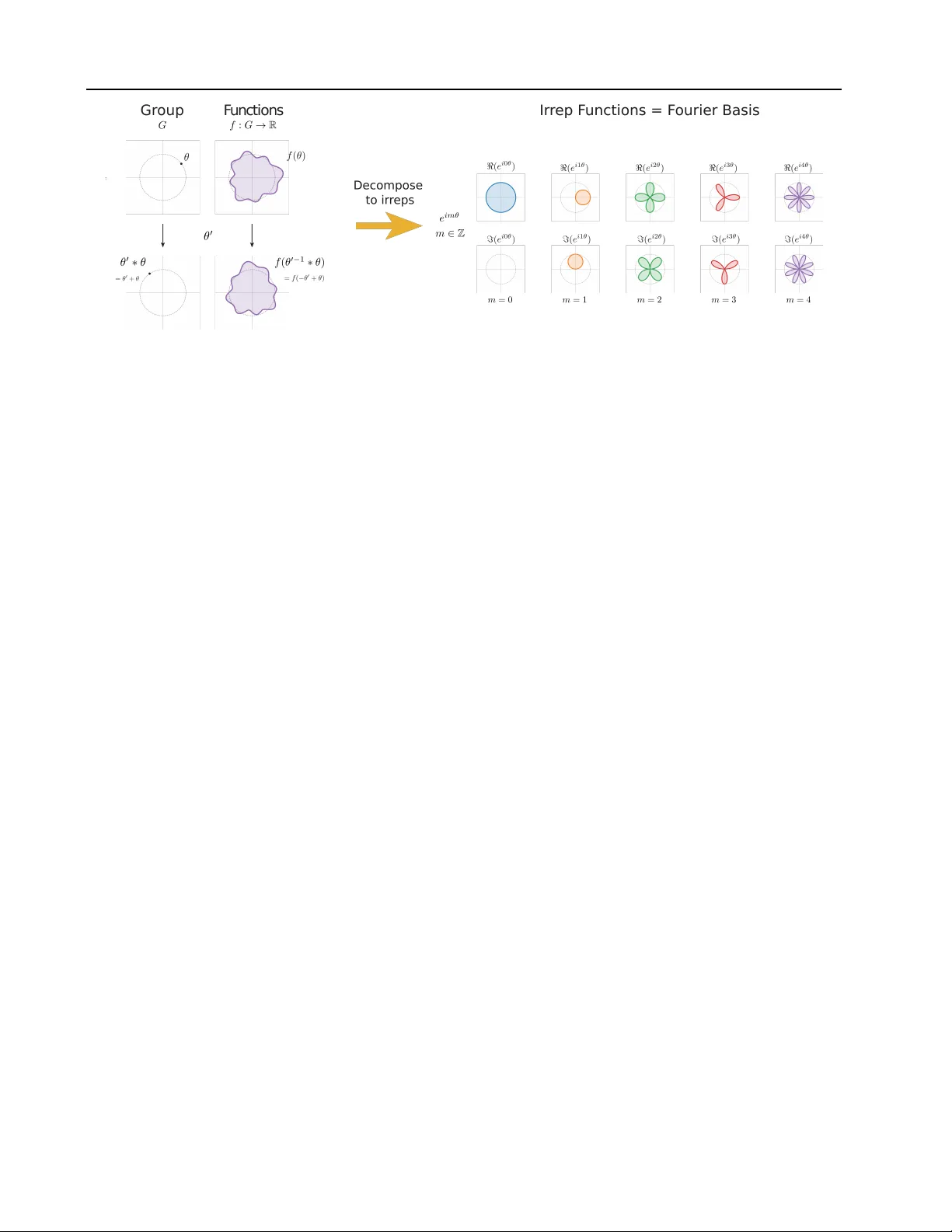
Asymptotically F ast Clebsch-Gordan T ensor Pr oducts with V ector Spherical Harmonics Y uQing Xie * 1 Ameya Daigav ane 1 Mit Kotak 2 T ess Smidt 1 Abstract E (3) -equiv ariant neural networks ha ve pro ven to be ef fectiv e in a wide range of 3D modeling tasks. A fundamental operation of such networks is the tensor product, which allows interaction between different feature types. Because this operation scales poorly , there has been considerable work tow ards accelerating this interaction. Howe v er , recently Xie et al. ( 2025 ) have pointed out that most speedups come from a reduction in expres- sivity rather than true algorithmic improv ements on computing Clebsch-Gordan tensor products. A modiﬁcation of Gaunt tensor product ( Luo et al. , 2024 ) can gi ve a true asymptotic speedup but is incomplete and misses many interactions. In this work, we provide the ﬁrst complete algorithm which truly provides asymptotic beneﬁts Clebsch- Gordan tensor products. For full CGTP , our algo- rithm brings runtime complexity from the nai ve O ( L 6 ) to O ( L 4 log 2 L ) , close to the lo wer bound of O ( L 4 ) . W e ﬁrst show ho w generalizing fast Fourier based con volution naturally leads to the previously proposed Gaunt tensor product ( Luo et al. , 2024 ). T o remedy antisymmetry issues, we generalize from scalar signals to irrep valued sig- nals, giving us tensor spherical harmonics. W e prov e a generalized Gaunt formula for the tensor harmonics. Finally , we show that we only need up to vector v alued signals to recover the missing interactions of Gaunt tensor product. 1. Introduction Symmetries are present in many complex ph ysical systems, and incorporating them in neural networks can signiﬁcantly improv e both learning ef ﬁciency and robustness ( Batzner 1 Department of EECS, Massachusetts Institute of T echnology , Cambridge, MA 02139, USA 2 Department of CSE, Massachusetts Institute of T echnology , Cambridge, MA 02139, USA. Corre- spondence to: Y uQing Xie < xyuqing@mit.edu > , T ess Smidt < tsmidt@mit.edu > . Pr eprint. F ebruary 26, 2026. et al. , 2022 ; Rackers et al. , 2023 ; Frey et al. , 2023 ; Owen et al. , 2024 ). As a result, considerable ef fort has been dedicated to dev elope E (3) -equiv ariant neural networks (E(3)NNs) ( Thomas et al. , 2018 ; W eiler et al. , 2018 ; K on- dor , 2018 ; K ondor et al. , 2018 ). E(3)NNs have deli vered strong performance across a wide range of scientiﬁc applica- tions, including molecular force ﬁelds ( Batzner et al. , 2022 ; Musaelian et al. , 2023 ; Batatia et al. , 2022 ), catalyst discov- ery ( Liao & Smidt , 2023 ), generativ e models ( Hoogeboom et al. , 2022 ), charge density prediction ( Fu et al. , 2024 ), and protein structure prediction ( Jumper et al. , 2021 ; Lee et al. , 2022 ). The group E (3) consists of all rotations, translations and reﬂections in 3 dimensions; we say a model is E (3) - equiv ariant if it satisﬁes: f ( g · x ) = g · f ( x ) ∀ g ∈ E (3) , x ∈ X . (1) The way a feature transforms under a group is called a group representation. For most groups of interest, a representa- tions can be broken into smaller pieces called irreducible representations (irreps). See Appendix B for a more in depth discussion. Hence, irreps are well studied objects in group theory and play a prominent role in many equiv ariant networks. It is useful to choose a basis where any representation is explicitly a direct sum of irreps. This is done in popular E (3) equi variant frame works ( Geiger & Smidt , 2022 ; Unke & Maennel , 2024 ; NVIDIA Corporation , 2025 ). Such a basis makes it easy to construct equiv ariant linear layers since Schur’ s Lemma tells us only irreps of the same type can mix. In order to interact irreps of dif ferent types, we can take a tensor product which is ef fecti vely an outer -product. Howe v er , the resulting representation is no longer explicitly a direct sum of irreps. The Clebsch-Gordan (CG) coef ﬁ- cients 1 ( V arshalovich et al. , 1988 ) provide the change of basis to con vert the resulting tensor product representation back into a direct sum of irreps. The combination of the outer product along with the CG change of basis is referred to as the Clebsch-Gordan tensor product (CGTP). 1 The v alues of the Clebsch-Gordan coefﬁcients are also basis dependent. In this paper we stick to quantum mechanical con- ventions. Most equiv ariant frameworks con vert to a real basis, changing the standard Clebsch-Gordan coefﬁcients. 1 Asymptotically Fast Clebsch-Gordan T ensor Pr oducts with V ector Spherical Harmonics Howe v er , CGTP is slo w , limiting our ability to scale up these models for lar ger systems. In the typical setting, it has been reported to have a time complexity of O ( L 6 ) ( Passaro & Zitnick , 2023 ) though it can be reduced to O ( L 5 ) by considering additional sparsity ( Cobb et al. , 2021 ). As a result, signiﬁcant effort to speed up equiv ariant networks has focused on tensor products. In molecular systems, one set of inputs for CGTP is often deriv ed from spherical harmonics of relative dif ference vec- tors. In this special case, Passaro & Zitnick ( 2023 ) showed a suitable rotation creates signiﬁcant sparsity allo wing for faster operations. Further , Li et al. ( 2025 ) reduces number of this type of tensor product needed from number of edges O ( |E | ) to number of vertices O ( |V | ) , allowing for better scaling on dense graphs. On the engineering side, there hav e been ef forts to b uild specialized kernels to optimize performance on current hard- ware. These include openEqui variance, FlashTP , cuEquiv- ariance, and B3 ( Bharadwaj et al. , 2025 ; Lee et al. , 2025 ; NVIDIA Corporation , 2025 ; K otak , 2025 ) which work for general tensor products. On the algorithmic side there ha ve been a number of al- ternativ es proposed. One line of work proposes working in a Cartesian basis instead of a strictly irrep (also called spherical) basis ( Shao et al. , 2024 ; Zav erkin et al. ). In this frame work taking tensor products is cheap, b ut decomposing back into irreps, especially to construct equiv ariant linear layers, now becomes e xpensiv e. Howe ver for CGTP , while these methods may be faster for small L , they hav e poor asymptotic scaling. There hav e also been alternati ve tensor product operations (TPOs) ( Luo et al. , 2024 ; Unke & Maennel , 2024 ) with better asymptotic scaling proposed to replace CGTP . Re- cently , Xie et al. ( 2025 ) pointed out that these alternati ves are not truly tensor products and their speedups directly come from reduced expressi vity . Using these to simulate full CGTP would lead to the same O ( L 5 ) scaling. Howe ver , Xie et al. ( 2025 ) noticed that there are asymptotically fast SH transform algorithms ( Healy et al. , 2003 ) which allo w the Gaunt tensor product (GTP) ( Luo et al. , 2024 ) to achie ve additional asymptotic runtime gains. These additional gains are the only truly algorithmic ones, not a result of losing expressi vity . Unfortunately , GTP is incomplete and misses interactions such as cross products and cannot fully simulate CGTP . In this paper , we present the ﬁrst TPO which truly provides asymptotic gains and is complete. It can be used to simulate full CGTP in O ( L 4 log 2 L ) time, close to the theoretical lower bound of O ( L 4 ) . W e present our results in a w ay which is generalizable to tensor products on other compact Lie groups. In addition, we provide a generalized version of the Gaunt formula for tensor spherical harmonics, which may be useful in other scientiﬁc ﬁelds. Our main contribu- tions are the following • First truly asymptotically faster and complete tensor product operation • A generalized Gaunt formula for tensor spherical har- monics • Explicit connection to group F ourier transforms, allo w- ing generalization to other groups • Drop-in replacement for Gaunt tensor product that is complete W e organize this paper as follo ws. In Section 2 , we brieﬂy cov er the frame work for analyzing tensor product operations introduced in Xie et al. ( 2025 ). In Section 3 , we draw an ex- plicit connection to group Fourier transforms, sho wing that the previously proposed Gaunt tensor product ( Luo et al. , 2024 ) is a natural result of attempting to generalize the ideas of fast Fourier based con volutions. In Section 4 , we gen- eralize from the usual scalar spherical harmonics to tensor spherical harmonics. W e show ho w to use tensor spherical harmonics to produce a TPO and deri ve generalized Gaunt coefﬁcients to analyze this operation. In Section 5 , we use this generalized formula to prove that we only need up to vector signals to perform any tensor product interaction, calling it vector signal tensor product (VSTP). Finally , in Section 6 , we summarize the asymptotic runtimes of our algorithm compared to other TPOs. 2. Analyzing tensor products A variety of tensor product operations (TPOs) hav e been proposed to accelerate the standard CGTP ( Unke & Maen- nel , 2024 ; Luo et al. , 2024 ). These can be deﬁned as the following. Deﬁnition 2.1 (T ensor product operations) . Let X, Y , Z be vector spaces equipped with actions of G . W e refer to any ﬁx ed equiv ariant bilinear T : X × Y → Z as a tensor product operation. Xie et al. ( 2025 ) then deﬁned an measure of expressi vity based for the TPOs. In fact, they sho w that all of the asymp- totic speed gains of pre viously proposed TPOs are directly explained by the loss in expressivity . Recovering the lost expressi vity would require multiple copies of these TPOs in parallel, resulting in asymptotic runtime equiv alent to standard CGTP with all sparsity constraints. Howe ver , it may be possible that certain CGTP interactions cannot be simulated no matter how many times we call a giv en TPO. For instance, GTP can ne ver simulate cross 2 Asymptotically Fast Clebsch-Gordan T ensor Pr oducts with V ector Spherical Harmonics products. ( Xie et al. , 2025 ) proposed a measure of inter- actibility to describe this issue. Their deﬁnition is equi valent to the following. Deﬁnition 2.2 (Interactability) . Let T : X × Y → Z be a tensor product operation. Let ( ℓ 1 , ℓ 2 , ℓ 3 ) be a triple of irrep types and V ℓ 1 , V ℓ 2 , V ℓ 3 be the corresponding spaces. Denote by Hom G ( A, B ) to be the set of equi variant linear maps from A → B . If there exists a nonzero bilinearity B : V ℓ 1 × V ℓ 2 → V ℓ 3 of the form B ( v 1 , v 2 ) = L Z ( T ( L X ( v 1 ) , L Y ( v 1 ))) where L X ∈ Hom G ( V ℓ 1 , X ) , L Y ∈ Hom G ( V ℓ 2 , Y ) , L Z ∈ Hom G ( Z, V ℓ 3 ) , then we say ( ℓ 1 , ℓ 2 , ℓ 3 ) is interactable under T . Intuiti vely , this just says ( ℓ 1 , ℓ 2 , ℓ 3 ) is interactable if we can use T to form a ℓ 3 type irrep from a pair of ℓ 1 , ℓ 2 inputs. GTP only allows even interactions where ℓ 1 + ℓ 2 + ℓ 3 is ev en. For example, cross product corresponds to (1 , 1 , 1) which has odd sum and is not computable. W e can directly analyze interactability by using selec- tion rules. Let the irreps in X, Y , Z be labeled by the tuples ( ℓ X , c X ) , ( ℓ Y , c Y ) and ( ℓ Z , c Z ) , where ℓ indi- cates the irrep type and c is an index over its multiplic- ity . A selection rule for T is a condition on the labels ( ℓ X , c X ) , ( ℓ Y , c Y ) , ( ℓ Z , c Z ) which must be satisﬁed for T | ( ℓ X ,c X ) , ( ℓ Y ,c Y ) , ( ℓ Z ,c Z ) : X ( ℓ X ,c X ) × Y ( ℓ Y ,c Y ) → Z ( ℓ Z ,c Z ) to be nonzero. If there is no choice of ( c X , c Y , c Z ) such that ( ℓ X , c X ) , ( ℓ Y , c Y ) and ( ℓ Z , c Z ) satisfy the selection rules for a giv en T , then ( ℓ 1 , ℓ 2 , ℓ 3 ) is not interactable under T . Hence, analyzing selection rules helps formally characterize which interactions are excluded by a speciﬁc TPO. For S O (3) (and S U (2) ), the triangle condition often ap- pears as a selection rule. Deﬁnition 2.3 (T riangle condition) . Let ( ℓ 1 , ℓ 2 , ℓ 3 ) be a triplet. They satisfy the triangle condition if ℓ 1 ≤ ℓ 2 + ℓ 3 ℓ 2 ≤ ℓ 1 + ℓ 3 ℓ 3 ≤ ℓ 1 + ℓ 2 . It is con venient to deﬁne the triangular delta as { ℓ 1 , ℓ 2 , ℓ 3 } = 1 if the abov e is satisﬁed and 0 otherwise. In particular , for single irrep CGTP the triangle condition is the only selection rule 2 . For GTP , we say there is an additional selection rule that ℓ 1 + ℓ 2 + ℓ 3 must be ev en. 3. Generalizing FFT con volutions In this section, we sho w how Gaunt tensor product naturally arises from attempting to generalize the ideas of FFT con vo- lution for use in tensor products. W e do so by ﬁrst looking 2 For multiple irreps we need to track the multiplicities at the natural generalization of Fourier transforms to com- pact nonabelian groups. There are then two natural ways to generalize the con volution theorem, either we consider group con volutions or we consider pointwise multiplication of group signals. The former establishes the connection between group equi variant con volution netw orks and irrep based equiv ariant networks, while the latter is promising for computing tensor products. Howe ver , group F ourier transforms have an unwieldy irrep multiplicity . By quoti- enting the group with an appropriate subgroup, we remov e redundant irreps. In the case of S O (3) , this quotient mani- fold is the sphere, giving us the spherical harmonics and the proposed Gaunt tensor product. 3.1. Group F ourier T ransforms In this context, a periodic function can be regarded as a sig- nal on S 1 . One can endow the circle with a group structure by addition of polar angle modulo 2 π to create the circle group T ∼ = S O (2) . The group action on the circle then in- duces an action on circle signals S 1 → C , namely a rotation by angle θ ′ rotates the signal f ( θ ) → f ′ ( θ ) = f ( θ − θ ′ ) . The set of circular signals forms a vector space and we can ask how it decomposes into irreps of T . These irreps cor- respond exactly to signals of the form e inθ , the standard Fourier basis. The F ourier coef ﬁcients are precisely the coefﬁcients obtained when we transform to this irrep basis. This connection between signals on a group and their irreps is generalized by the Peter W eyl theorem. Theorem 3.1 (Peter -W eyl Theorem) . Let G be a compact topological gr oup. Let Σ contain exactly one r epresentative irr ep fr om each isomorphism class of irreps. F or each irr ep π ∈ Σ , denote by D ( π ) the corresponding matrix for the irr ep written in an orthonormal basis. Then the space of squar e-inte grable functions L 2 ( G ) has an orthonormal basis consisting of { p d π D ( π ) ij | π ∈ Σ , 1 ≤ i, j ≤ d π } In the case of S O (3) , this means an orthonormal basis for S O (3) is giv en by the elements in the Wigner -D matrices scaled appropriately . W e similarly then hav e generalized Fourier transform (GFT) coef ﬁcients obtained when trans- forming into this orthonormal basis. Due to orthonormality we can compute these as M ( π ) ij ( f ) = Z G p d π f ( g ) D ( π ) ij ( g ) dµ ( g ) where f : G → C is our signal and µ is the Haar measure. 3.2. Generalizing Con volution Theorems For the usual F ourier transform of periodic functions, there are two con volution theorems. One states that con volution 3 Asymptotically Fast Clebsch-Gordan T ensor Pr oducts with V ector Spherical Harmonics F igure 1. Fourier transforms from a group theoretic perspective. An action on a group induces an action on functions on the group. These functions form a v ector space and hence this deﬁnes a group representation. W e can decompose this representation into irreps, gi ving exactly the standard F ourier basis. The Peter-W eyl theorem generalizes this idea for compact Lie groups. of two circular signals gi ves pointwise multiplication on the coefﬁcients. The other states pointwise multiplication of two circular signals gi ves conv olution on the coef ﬁcients. So there are tw o natural w ays to generalize for compact groups. W e can either perform con volution of two group signals or pointwise multiplication of two group signals. Con volution of two group signals has been extensi vely ex- plored in prior work and forms the basis of early equi variant models ( Cohen & W elling , 2016 ; Cohen et al. , 2018 ). The Fourier coef ﬁcients naturally organize into matrices, corre- sponding exactly into the matrices forming the orthonormal basis. The group con volution then becomes matrix multi- plication of the coef ﬁcients ( K ostelec & Rockmore , 2008 ; Cohen et al. , 2018 ). In group conv olution networks, we typ- ically vie w one signal as our features and the other signal as a ﬁlter . In irrep focused frame works such as e3nn ( Geiger & Smidt , 2022 ), the Fourier coef ﬁcients of the features con- sist of d ℓ copies of irreps of type ℓ and the coefﬁcients of the ﬁlter correspond to in variant weights for an equi variant linear layer . Less explored in equiv ariant literature is pointwise multi- plication of two group signals. T o understand the resulting action on the Fourier coef ﬁcients, one must understand how the product of the basis matrices decompose. In the case of S O (3) , this is gi ven by D ( ℓ 1 ) m 1 n 1 ( g ) D ( ℓ 2 ) m 2 n 2 ( g ) = X ℓ 3 C ℓ 3 ,m 1 + m 2 ℓ 1 ,m 1 ,ℓ 2 ,m 2 C ℓ 3 ,n 1 + n 2 ℓ 1 ,n 1 ,ℓ 2 ,n 2 D ( ℓ 3 ) m 1 + m 2 ,n 1 + n 2 ( g ) (2) where here we use the typical con vention that indices m i , n i ∈ {− ℓ, − ℓ + 1 , . . . , ℓ − 1 , ℓ } . Note the appearance of the Clebsch-Gordan coef ﬁcients which is promising. This formula generalizes to other Lie groups where we replace the W igner D with the corresponding irrep matrix and the Clebsch-Gordan coefﬁcients with those for the other group. Note ho wev er that for S O (3) there are d ℓ = 2 ℓ + 1 copies of irreps of type ℓ . This is rather unwieldy . Further , the cor- responding GFT scales poorly . The corresponding Nyquist sampling theorem requires number of points scaling as L 3 . Hence it infeasible to use this to speed up tensor products of a pair of single irreps and we must use multiple input irreps to possibly achie ve better asymptotic runtime/expressi vity ratios. 3.3. Reduction to Spherical Signals Here, we describe how quotienting the S O (3) manifold reduces the irrep multiplicity , giving us the sphere S 2 . This lets us derive the Gaunt coef ﬁcients and sho ws how the Gaunt tensor product is a natural consequence of trying to generalize the key idea of FFT con volutions. This also lets us generalize the process for arbitrary Lie groups and giv es the analog of the sphere. Consider the S O (2) subgroup generated by rotations about the z axis. Then we can take the left cosets to create the quotient manifold S O (3) /S O (2) ∼ = S 2 where the equi va- lence to S 2 is a well kno wn correspondence. T o deriv e the spherical harmonics from a representation theory perspec- tiv e, we realize that there are two natural group actions on S O (3) itself. W e can either perform group multiplication on the left or on the right. That is g ′ acting on g either giv es g → g ′ g or g → g g ′ . Depending on whether we choose left or right multiplication, the induced action on the S O (3) sig- nals changes and the d ℓ copies of irrep ℓ are giv en either by the columns or rows respecti vely of the W igner D matrices. Next, we note that the indices m, n describe exactly ho w much that component changes under z rotations. That is if g z ( θ ) is a rotation about z by angle θ , we have D ( ℓ ) m,n ( g g z ( θ )) = D ( ℓ ) m,n ( g ) e inθ D ( ℓ ) m,n ( g z ( θ ) g ) = D ( ℓ ) m,n ( g ) e imθ 4 Asymptotically Fast Clebsch-Gordan T ensor Pr oducts with V ector Spherical Harmonics If we quotient out by z rotations acting on the right (giving left cosets), that means we need n = 0 to obtain func- tions which are in variant under z rotations. This means D ( ℓ ) m, 0 ( g g z ) = D ( ℓ ) m, 0 ( g ) for all g z ∈ S O (2) and hence we expect D ( ℓ ) m, 0 to form a basis for S O (3) /S O (2) . It turns out that D ( ℓ ) m, 0 ( g ) = r 4 π 2 ℓ + 1 Y m, ∗ ℓ ( g ˆ z ) so the W igner D matrices indeed reduce to the spherical harmonics 3 . By substituting this relation into equation 2 , we obtain Y m 1 , ∗ ℓ 1 ( g ˆ z ) Y m 1 , ∗ ℓ 1 ( g ˆ z ) = s (2 ℓ 1 + 1)(2 ℓ 2 + 1) 4 π (2 ℓ 3 + 1) × X ℓ 3 C ℓ 3 ,m 1 + m 2 ℓ 1 ,m 1 ,ℓ 2 ,m 2 C ℓ 3 , 0 ℓ 1 , 0 ,ℓ 2 , 0 Y m 1 + m 2 , ∗ ℓ 3 ( g ˆ z ) . These are exactly the Gaunt coef ﬁcients ( Gaunt , 1929 ). Hence, we see that the Gaunt tensor product is what natu- rally arises when trying to exploit the pointwise multipli- cation analog of the con volution theorem for compact lie groups and then trying to form a quotient manifold to reduce the irrep multiplicity . It turns out S O (2) is called a maximal torus and for general Lie groups, we can also quotient by a maximal torus to eliminate irrep multiplicity . Howe ver , as also pointed by Xie et al. ( 2025 ) Gaunt tensor product suffers from an antisymmetry problem and many interactions such as cross products are not possible. In ad- dition, the procedure of quotienting out the maximal torus does not guarantee ev ery irrep is present in the correspond- ing harmonics. For example for S U (2) , the maximal torus is U (1) and we still hav e S U (2) /U (1) ∼ = S 2 . Hence we still only obtain the spherical harmonics and inte ger repre- sentations, missing all the half integer representations of S U (2) . 4. Generalizing Spherical Harmonics T o remedy the antisymmetry issue, we must generalize the spherical harmonics in a suitable way . In physics literature, there are two types of generalizations: spin weighted spher- ical harmonics (SWSH) and tensor spherical harmonics (TSH). The former were introduced by Newman & Penrose ( 1966 ) to study gravitational wav es and also e xplored in the equiv ariant literature as a way to generalize spherical CNNs ( Este ves et al. , 2020 ). The latter is a decomposition of tensor valued signals on the sphere. The vector spherical 3 Throughout this paper , we use quantum mechanical con ven- tions and our spherical harmonics are complex. This also f acilitates analysis. The real spherical harmonics are related by a basis change and hence our main results still follow . harmonics in particular play an important role in man y ar- eas of physics ( Barrera et al. , 1985 ; Carrascal et al. , 1991 ; Moses , 1974 ; W einberg , 1994 ). The spin-weighted and ten- sor harmonics are intimately related and we believe both can be used to solve the antisymmetry issue ( Thorne , 1980 ; Ledesma & Me wes , 2020 ). In this work, we will focus on tensor harmonics. 4.1. T ensor Spherical Harmonics Suppose instead of a scalar signal, we instead have a tensor valued signal which transforms under some group represen- tation. Since any representation can be decomposed as a sum of irreps, we can consider only irrep v alued signals. Now when we act on such a signal, we must also transform the output. That is, any irrep s signal f s : S 2 → R 2 s +1 transforms as f s ( x ) → D ( s ) ( g ) f s ( g − 1 x ) . W e can then similarly ask ho w to decompose the vector space of such signals into a direct sum of irreps and form an orthonormal basis. W e can interpret the transformation of irrep signals as a tensor product representation of a transform acting on the inputs, and a transform acting on the outputs. The spheri- cal harmonics already tell us how to decompose the input transformation into irreps while the output representation is assumed to be an irrep. Therefore, to reduce the over - all transformation into irreps, we can simply just use the Clebsch-Gordan decomposition. This leads to the following deﬁnition of tensor spherical harmonics. Deﬁnition 4.1 (T ensor spherical harmonics) . For integers j, ℓ, s, m where | j − 1 | ≤ ℓ ≤ j + 1 and | m j | ≤ j , we deﬁne the functions Y ℓ,s j,m j : S 2 → R 2 s +1 as ( Y ℓ,s j,m j ( ˆ r )) m s = X m ℓ C j,m j ℓ,m ℓ ,s,m s Y m ℓ ℓ ( ˆ r ) . W e refer to these functions as the tensor spherical harmonics (TSH). In physics, ℓ is typically interpreted as orbital angular mo- mentum, s as spin, and j as total angular momentum. Note that the TSH transforms as an irrep of type j . Remark 4.2 . W e would like to point out that this choice for TSH is not unique. Ours is the most natural choice from a representation theory perspectiv e, howe ver there may be other choices that are natural for dif ferent contexts. For instance, s = 1 giv es the vector spherical harmonics. Howe ver , the outputs of Y j − 1 , 1 j,m and Y j +1 , 1 j,m are not purely perpendicular or tangent to the local tangent plane. Hence, one often sees an alternativ e basis consisting of purely radial, curl-free, and div ergence free components. 5 Asymptotically Fast Clebsch-Gordan T ensor Pr oducts with V ector Spherical Harmonics 4.2. Computing TSH transform Because Deﬁnition 4.1 relates the TSH to regular scalar SHs, we can compute a forward TSH transform by performing multiple regular SH transforms and performing a Clebsch- Gordan decomposition on the resulting coef ﬁcients to obtain the TSH coef ﬁcients. For the reverse TSH transform, we can similarly use Clebsch-Gordan coefﬁcients to transform into multiple regular SH coef ﬁcients and then just perform multiple rev erse SH transforms. Because we no w compute multiple SH transforms and we compute a Clebsch-Gordan decomposition, the abo ve pro- cedure adds a complexity factor that depends on the chosen spin s . Howe ver as we shall see in Section 5 , we only need up to s = 1 to be able to compute any tensor product. 4.3. Irrep signal tensor pr oduct Giv en any two tensors, the most general bilinear interaction is a tensor product. Therefore, giv en any two irrep signals, the most general interaction is to perform a pointwise tensor product. The resulting signal output transforms as a tensor product representation. W e can then use the Clebsch-Gordan decomposition to change to an irrep basis. In particular, if we hav e irrep signals f s 1 and f s 2 and desire a resulting irrep signal of type s 3 , we can get ( f s 1 ⊗ f s 2 ) s 3 m 3 ( ˆ r ) = X m 1 ,m 2 C s 3 ,m 3 s 1 ,m 1 ,s 2 ,m 2 f s 1 m 1 ( ˆ r ) f s 2 m 2 ( ˆ r ) . If s 1 = s 2 = s 3 = 0 , the abo ve operation is the usual pointwise multiplication of scalar signals. Using this interaction, we can now deﬁne a general class of TPOs we call irrep signal tensor products (ISTPs). For any triplet ( s 1 , s 2 , s 3 ) , we can perform the following 1. Interpret input irreps labeled by ( j i , ℓ i ) as coefﬁcients for a set of TSHs Y ℓ i ,s i j i . 2. Do a reverse TSH transform to form a tensor signal f s i = X j i ,ℓ i ,m i ( x i ) ( j i ,ℓ i ) m i Y ℓ i ,s i j i ,m i . 3. Compute pointwise tensor products to obtain f s 3 = ( f s 1 ⊗ f s 2 ) s 3 . 4. Finally , we perform a TSH transform on f s 3 to get corresponding TSH coefﬁcients labeled by ( j 3 , ℓ 3 ) . Note that the (0 , 0 , 0) version corresponds to Gaunt tensor product. 4.4. Generalized Gaunt formula T o analyze the ISTP procedure, we need a formula to de- compose 2 TSHs. Theorem 4.3. W e have the following decomposition of ten- sor spherical harmonics ( Y ℓ 1 ,s 1 j 1 ,m 1 ⊗ Y ℓ 2 ,s 2 j 2 ,m 2 ) s 3 = r (2 j 1 + 1)(2 j 2 + 1)(2 ℓ 1 + 1)(2 ℓ 2 + 1)(2 s 3 + 1) 4 π X j 3 ,ℓ 3 ,m 3    j 1 ℓ 1 s 1 j 2 ℓ 2 s 2 j 3 ℓ 3 s 3    C ℓ, 0 ℓ 1 , 0 ,ℓ 2 , 0 C j 3 ,m 3 j 1 ,m 1 ,j 2 ,m 2 Y ℓ 3 ,s 3 j 3 ,m 3 . Here, the 3 × 3 curly brace denotes the W igner 9j symbol deﬁned in Deﬁnition F .3 . Pr oof sketch. T o compute the signal at each point, we ﬁrst couple our TSH coef ﬁcient of type j i with a spherical har - monic of type ℓ i to form a resulting s i . W e then couple s 1 , s 2 to form the ﬁnal s 3 . This is a speciﬁc choice to couple 4 irreps of type ℓ 1 , j 1 , ℓ 2 , j 2 . Howe ver , we can al- ternativ ely couple ℓ 1 , ℓ 2 to form ℓ 3 and j 1 , j 2 to form j 3 before coupling ℓ 3 , j 3 to form s 3 . The Wigner 9j gi ves the change of basis between these coupling orders. In the latter, the ℓ 1 , ℓ 2 coupling gives a ℓ 3 spherical harmonic and the j 1 , j 2 coupling giv es the desired CGTP coef ﬁcients. The last ℓ 3 , j 3 coupling is exactly a TSH coupling giving the ﬁnal Y j 3 ,m 3 ℓ 3 ,s 3 . Full proof is in Section F .1 . Remark 4.4 . T o the best of our knowledge, this general formula and our deriv ation method is nov el. V ersions for s ≤ 1 can be found in V arshalovich et al. ( 1988 ). 5. V ector Signals is All Y ou Need In this section, we prove only up to s = 1 is needed to perform all possible tensor product interactions. In partic- ular , we focus on the (1 , 1 , 1) ISTP which is equiv alent to performing cross products of vector spherical signals (up to a factor of √ 2 ). W e call this vector signal tensor product (VSTP). W e then derive the corresponding selection rules and then prove one always has an interaction. Finally , we show a constant number of VSTPs can be used to simulate computing full CGTP of a pair of irreps. 5.1. V ector signal tensor pr oduct Here, we consider s = 1 signals, which corresponds to vector signals on the sphere. Inspecting the Clebsch-Gordan coefﬁcients, one can sho w that ( f (1) ⊗ g (1) ) (1) m 3 = − 1 √ 2 ( f (1) × g (1) ) m 3 so the interaction is proportional to taking a cross product. 6 Asymptotically Fast Clebsch-Gordan T ensor Pr oducts with V ector Spherical Harmonics F igure 2. Schematic of the process in taking a vector signal tensor product. W e interpret input irreps as vector SH coef ﬁcients to create vector spherical signals. W e then take pointwise cross products of the two signals to create a ne w signal which we decompose back into vector SH coef ﬁcients. 5.2. Selection rules and completeness Using Theorem 4.3 , we can derive selection rules for VSTP . Theorem 5.1 (Selection rules for VSTP) . Consider irr ep labels j 1 , ℓ 1 , j 2 , ℓ 2 , j 3 , ℓ 3 . The corr esponding interaction is nonzer o if and only if the following are satisﬁed: 1. { j 1 , ℓ 1 , 1 } = { j 2 , ℓ 2 , 1 } = { j 3 , ℓ 3 , 1 } = 1 2. { j 1 , j 2 , j 3 } = 1 3. { ℓ 1 , ℓ 2 , ℓ 3 } = 1 4. ℓ 1 + ℓ 2 + ℓ 3 is even 5. Ther e is no c hoice of distinct a, b, c such that j a = ℓ a and ( j b , ℓ b ) = ( j c , ℓ c ) Pr oof sketch. Rules 1-3 follo w from the fact that the trian- gle condition must be satisﬁed in the rows and columns of the W igner 9j symbol. Rule 5 follows from the (anti)symmetry relation of the W igner 9j under odd row or column permutations. Rule 4 follo ws from the even selection rule of the C ℓ 3 , 0 ℓ 1 , 0 ,ℓ 2 , 0 coefﬁcient. T o show these are always nonzero, one looks at the ex- plicit expressions of the W igner 9j symbols documented in V arshalovich et al. ( 1988 ). T edious inspection of these coef- ﬁcients then sho w that they only become zero when it fails the selection rules 1-4. Finally , it is known that C ℓ, 0 ℓ 1 , 0 ,ℓ 2 , 0 is nonzero if and only if it satisﬁes rule 5 ( Raynal , 1978 ). Full proof is in Section F .2 . In contrast to GTP , VSTP selection rules allow all the possi- ble paths except for multiplication of scalars. Theorem 5.2. Suppose { j 1 , j 2 , j 3 } = 1 and the j ′ s ar e not all 0. Then ( j 1 , j 2 , j 3 ) is interactable under a VSTP of sufﬁciently high de gr ee. Pr oof sketch. W e perform tedious casework on the possible ℓ i for each j i and sho w we can alw ays ﬁnd some ℓ 1 , ℓ 2 , ℓ 3 such that j 1 , ℓ 1 , j 2 , ℓ 2 , j 3 , ℓ 3 satisﬁes the selection rules of Theorem 5.1 . Full proof is in Section F .3 . 5.3. Simulating CGTP with VSTP Corollary 5.3. Suppose we have a pair of inputs of irrep types j 1 , j 2 . W e can compute ( x ( j 1 ) ⊗ x ( j 2 ) ) ( j 3 ) with a constant number of VSTPs. Pr oof. If j 1 = j 2 = j 3 = 0 , then they are all scalars and we multiply using no VSTPs. Each input j i has up to 3 possible ℓ i it can be paired with. W e simply compute a VSTP for each possible combination j 1 , ℓ 1 and j 2 , ℓ 2 . There are at most 3 · 3 = 9 such combina- tions. By Theorem 5.2 , there is at least one j 3 , ℓ 3 that works with one of the the computed VSTPs. 6. Asymptotic runtimes and expressi vity 6.1. Expressi vity runtime tradeoffs W e analyzed the asymptotic runtimes and expressivity re- spectiv ely in Appendix D and Appendix E of ISTP and VSTP . The results are summarized in T able 1 . For expres- sivity , we assume we are using the v arious tensor products to construct bilinearities from space X = Y transforming as (0 ⊕ . . . ⊕ L ) to space Z transforming as (0 ⊕ . . . ⊕ 2 L ) . Note that because s = 1 is a ﬁnite cutoff, VSTP has the same asymptotics as GTP . 6.2. CGTP simulation By Corollary 5.3 , we can fully simulate CGTP for a pair of irreps with a constant number of VSTPs. In the setting where both inputs are of type (0 ⊕ . . . ⊕ L ) , there are ( L + 1) 2 = O ( L 2 ) ways to pair input irreps. Hence, we need O ( L 2 ) VSTP calls to simulate the corresponding CGTP . Since each VSTP call runs in O ( L 2 log 2 L ) time, this giv es O ( L 4 log 2 L ) runtime to fully simulate CGTP . 7 Asymptotically Fast Clebsch-Gordan T ensor Pr oducts with V ector Spherical Harmonics T able 1. Asymptotic runtimes and expressi vity of various tensor product implementations. Note that the fast spherical transform algorithm by Healy et al. ( 2003 ) giv es the best runtime/expressi vity tradeoff ratios. T ensor Product Expressivity Runtime Runtime / Expressivity CGTP (Naiv e) O ( L 3 ) O ( L 6 ) O ( L 3 ) CGTP (Sparse) O ( L 3 ) O ( L 5 ) O ( L 2 ) GTP (Fourier) O ( L ) O ( L 3 ) O ( L 2 ) GTP (Grid) O ( L ) O ( L 3 ) O ( L 2 ) GTP (Healy) O ( L ) O ( L 2 log 2 L ) O ( L log 2 L ) VSTP (Grid) O ( L ) O ( L 3 ) O ( L 2 ) VSTP (Healy) O ( L ) O ( L 2 log 2 L ) O ( L log 2 L ) ISTP (Grid) O ( ˜ sL ) O ( ˜ s 2 L 2 + ˜ sL 3 ) O ( ˜ sL + L 2 ) ISTP (S2FFT) O ( ˜ sL ) O ( ˜ s 2 L 2 + ˜ sL 2 log 2 L ) O ( ˜ sL + L log 2 L ) 7. Limitations While our work presents the ﬁrst asymptotic improvements for computing full CGTP , it is not practical for the L ’ s currently used in equiv ariant networks. In the spherical har- monic transform, asymptotically fast O ( L 2 log 2 L ) versions often suf fer from numerical stability compared to O ( L 3 ) versions. In addition, runtime beneﬁts for fast SH trans- forms are often only achie ved for L ∼ 1000 , far higher than any L currently used in E(3)NNs. Howe ver , there are many domains which use e xtremely high L . For instance, the Earth Gra vitation Model uses L ∼ 2000 ( Pa vlis et al. , 2008 ) and planetary topography models go up to L ∼ 40 , 000 ( Rex er & Hirt , 2015 ). It may be possible that the ideas in this paper will be useful in the f ar future for such domains. Lastly , it is possible VSTP with O ( L 3 ) SH transforms is viable on current equiv ariant networks. It would be quite similar to the already viable GTP with a constant factor increase in expressivity , no interactibility problems, but also constant factor speed decrease. Howe ver , we hav e not robustly tested our preliminary implementation. In addi- tion, many common benchmarks compute quantities such as forces or energies which can already be formed from the interactions of GTP . Hence, the lost interactibility of GTP may not be an issue in such tasks. 8. Conclusion In this work, we in vestigated the use of spherical signals to perform Clebsch-Gordan tensor products. W e ﬁrst e xplicitly drew connections to group F ourier transforms, sho wing ho w a natural extension of FFT ideas to compute conv olutions leads to GTP . W e then sho wed that by generalizing to tensor spherical signals, we can obtain new types of interactions and circumvent antisymmetry issues. W e derived a gen- eralized Gaunt formula for tensor harmonics under these interactions. Next, we sho wed only up to vector spherical harmonics is necessary to fully simulate CGTP . Finally , we analyzed the asymptotics of our proposed VSTP , sharing the same beneﬁts as GTP from fast SH transforms but not suffering from interactibility issues. For future work, we would lik e to robustly test the viability of VSTP in actual E(3)NNs. This may require careful ini- tialization and normalization which our generalized Gaunt formula can help analyze. Further, we believe it will be fruitful to explore spin-weighted spherical harmonics, the other possible generalization of scalar SH. Acknowledgments Y uQing Xie, Ameya Daigav ane, and Mit K otak were sup- ported by the NSF Graduate Research Fellowship program under Grant No. DGE-1745302. W e were also supported by the U.S. Department of Energy , Ofﬁce of Science, under A ward No. DE-SC0026242, Hierarchical Representations of Complex Physical Systems with Euclidean Neural Net- works and the National Science Foundation under Cooper - ativ e Agreement PHY -2019786 (The NSF AI Institute for Artiﬁcial Intelligence and Fundamental Interactions). Impact Statement This paper presents work whose goal is to advance the ﬁeld of Machine Learning. There are many potential societal consequences of our work, none which we feel must be speciﬁcally highlighted here. References Barrera, R. G., Estev ez, G., and Giraldo, J. V ector spher- ical harmonics and their application to magnetostatics. Eur opean Journal of Physics , 6(4):287, 1985. Batatia, I., Ko vacs, D. P ., Simm, G. N. C., Ortner, C., and Csanyi, G. MA CE: Higher Order Equiv ariant Message Passing Neural Networks for Fast and Accurate Force Fields. In Oh, A. H., Agarw al, A., Belgrav e, D., and Cho, K. (eds.), Advances in Neural Information Pr ocessing Systems , 2022. URL https://openreview . net/ forum?id=YPpSngE- ZU . Batzner , S., Musaelian, A., Sun, L., Geiger , M., Mailoa, J. P ., K ornbluth, M., Molinari, N., Smidt, T . E., and Kozin- sky , B. E(3)-equi variant graph neural networks for data- efﬁcient and accurate interatomic potentials. 13, May 2022. URL https://doi . org/10 . 1038/s41467- 022- 29939- 5 . Bharadwaj, V ., Glo ver , A., Bulu c ¸ , A., and Demmel, J. An ef ﬁcient sparse kernel generator for o (3)-equiv ariant deep networks. In 2025 Pr oceedings of the Confer ence on Applied and Computational Discr ete Algorithms (ACD A) , pp. 32–46. SIAM, 2025. 8 Asymptotically Fast Clebsch-Gordan T ensor Pr oducts with V ector Spherical Harmonics Carrascal, B., Estevez, G., Lee, P ., and Lorenzo, V . V ec- tor spherical harmonics and their application to classical electrodynamics. European Journal of Physics , 12(4): 184, 1991. Cobb, O., W allis, C., Mav or-Parker , A., Marignier , A., Price, M., D’A vezac, M., and McEwen, J. Efﬁcient generalized spherical cnns. In ICLR 2021-9th International Con- fer ence on Learning Repr esentations , volume 9. ICLR 2021-9th International Conference on Learning Repre- sentations, 2021. Cohen, T . and W elling, M. Group equiv ariant conv olutional networks. In International confer ence on machine learn- ing , pp. 2990–2999. PMLR, 2016. Cohen, T . S., Geiger, M., K ¨ ohler , J., and W elling, M. Spher - ical cnns. In International Confer ence on Learning Rep- r esentations , 2018. Dresselhaus, M. S., Dresselhaus, G., and Jorio, A. Gr oup theory: application to the physics of condensed matter . Springer Science & Business Media, 2007. Estev es, C., Makadia, A., and Daniilidis, K. Spin-weighted spherical cnns. Advances in Neural Information Pr ocess- ing Systems , 33:8614–8625, 2020. Frey , N. C., Soklaski, R., Axelrod, S., Samsi, S., G ´ omez- Bombarelli, R., Coley , C. W ., and Gadepally , V . Neural scaling of deep chemical models. Natur e Machine Intelli- gence , 5(11):1297–1305, October 2023. Fu, X., Rosen, A., Bystrom, K., W ang, R., Musaelian, A., K ozinsky , B., Smidt, T ., and Jaakkola, T . A recipe for charge density prediction, 2024. Gaunt, J. A. Iv . the triplets of helium. Philosophical T rans- actions of the Royal Society of London. Series A, Con- taining P apers of a Mathematical or Physical Character , 228(659-669):151–196, 1929. Geiger , M. and Smidt, T . e3nn: Euclidean neural networks. arXiv pr eprint arXiv:2207.09453 , 2022. Healy , D. M., Rockmore, D. N., K ostelec, P . J., and Moore, S. FFTs for the 2-sphere-improvements and variations. Journal of F ourier analysis and applications , 9:341–385, 2003. Hoogeboom, E., Satorras, V . G., V ignac, C., and W elling, M. Equi variant dif fusion for molecule generation in 3d, 2022. Jumper , J., Evans, R., Pritzel, A., Green, T ., Figurnov , M., Ronneberger , O., T unyasuvunakool, K., Bates, R., ˇ Z ´ ıdek, A., Potapenko, A., Bridgland, A., Me yer , C., Kohl, S. A. A., Ballard, A. J., Cowie, A., Romera-Paredes, B., Nikolov , S., Jain, R., Adler , J., Back, T ., Petersen, S., Reiman, D., Clancy , E., Zielinski, M., Steinegger , M., Pacholska, M., Berghammer , T ., Bodenstein, S., Silver , D., V inyals, O., Senior , A. W ., Kavukcuoglu, K., K ohli, P ., and Hassabis, D. Highly accurate protein structure prediction with alphafold. Natur e , 596(7873):583–589, 2021. K ondor , R. N-body networks: a covariant hierarchi- cal neural network architecture for learning atomic po- tentials, 2018. URL https://arxiv . org/abs/ 1803 . 01588 . K ondor , R., Lin, Z., and Tri vedi, S. Clebsch-gordan nets: a fully fourier space spherical conv olutional neural netw ork. Advances in Neural Information Pr ocessing Systems , 31, 2018. K ostelec, P . J. and Rockmore, D. N. Ffts on the rotation group. J ournal of F ourier analysis and applications , 14 (2):145–179, 2008. K otak, M. Simplifying equivariant gpu kernels through tile-based programming. Master’ s thesis, MAS- SA CHUSETTS INSTITUTE OF TECHNOLOGY , 2025. Ledesma, F . G. and Mewes, M. Spherical-harmonic tensors. Physical Revie w Resear ch , 2(4):043061, 2020. Lee, J. H., Y adollahpour , P ., W atkins, A., Frey , N. C., Leav er-F ay , A., Ra, S., Cho, K., Gligorije vic, V ., Rege v , A., and Bonneau, R. Equifold: Protein structure predic- tion with a nov el coarse-grained structure representation. bioRxiv , 2022. doi: 10 . 1101/2022 . 10 . 07 . 511322. URL https://www . biorxiv . org/content/early/ 2022/10/08/2022 . 10 . 07 . 511322 . Lee, S. Y ., Kim, H., Park, Y ., Jeong, D., Han, S., Park, Y ., and Lee, J. W . Flashtp: Fused, sparsity-aw are ten- sor product for machine learning interatomic potentials. In F orty-second International Conference on Mac hine Learning . PMLR, 2025. Li, Y ., Huang, L., Ding, Z., W ei, X., W ang, C., Y ang, H., W ang, Z., Liu, C., Shi, Y ., Jin, P ., et al. E2former: An efﬁcient and equi variant transformer with linear-scaling tensor products. In The Thirty-ninth Annual Confer ence on Neural Information Pr ocessing Systems , 2025. Liao, Y .-L. and Smidt, T . Equiformer: Equi variant graph attention transformer for 3d atomistic graphs. In The Eleventh International Confer ence on Learning Repre- sentations , 2023. URL https://openreview . net/ forum?id=KwmPfARgOTD . Luo, S., Chen, T ., and Krishnapriyan, A. S. Enabling efﬁ- cient equiv ariant operations in the fourier basis via gaunt tensor products. arXiv pr eprint arXiv:2401.10216 , 2024. 9 Asymptotically Fast Clebsch-Gordan T ensor Pr oducts with V ector Spherical Harmonics Moses, H. The use of v ector spherical harmonics in global meteorology and aeronomy . J ournal of Atmospheric Sci- ences , 31(6):1490–1499, 1974. Musaelian, A., Batzner , S., Johansson, A., Sun, L., Owen, C. J., K ornbluth, M., and K ozinsky , B. Learning local equiv ariant representations for large-scale atomistic dy- namics. Natur e Communications , 14(1):579, 2023. Newman, E. T . and Penrose, R. Note on the bondi-metzner- sachs group. Journal of Mathematical Physics , 7(5): 863–870, 1966. NVIDIA Corporation. cuequivariance. https: //docs . nvidia . com/cuda/cuequivariance/ , 2025. Accessed: 2026-01-22. Owen, C. J., T orrisi, S. B., Xie, Y ., Batzner , S., Bystrom, K., Coulter , J., Musaelian, A., Sun, L., and K ozinsky , B. Complexity of many-body interactions in transition metals via machine-learned force ﬁelds from the TM23 data set. Npj Comput. Mater . , 10(1), May 2024. Passaro, S. and Zitnick, C. L. Reducing so (3) con volu- tions to so (2) for efﬁcient equiv ariant gnns. In Inter- national Conference on Machine Learning , pp. 27420– 27438. PMLR, 2023. Pa vlis, N., K enyon, S., Factor , J., and Holmes, S. Earth gravitational model 2008. In SEG technical pr ogram expanded abstr acts 2008 , pp. 761–763. Society of Explo- ration Geophysicists, 2008. Rackers, J. A., T ecot, L., Geiger , M., and Smidt, T . E. A recipe for cracking the quantum scaling limit with ma- chine learned electron densities. Mac h. Learn.: Sci. T ech- nol. , 4(1):015027, February 2023. Raynal, J. On the deﬁnition and properties of generalized 3-j symbols. Journal of Mathematical Physics , 19(2): 467–476, 1978. Rex er , M. and Hirt, C. Ultra-high-de gree surface spheri- cal harmonic analysis using the gauss–le gendre and the driscoll/healy quadrature theorem and application to plan- etary topography models of earth, mars and moon. Sur- ve ys in Geophysics , 36(6):803–830, 2015. Shao, S., Li, Y ., Lin, Z., and Cui, Q. High-rank irreducible cartesian tensor decomposition and bases of equi variant spaces. arXiv pr eprint arXiv:2412.18263 , 2024. Thomas, N., Smidt, T ., Kearnes, S., Y ang, L., Li, L., K ohlhoff, K., and Riley , P . T ensor ﬁeld networks: Rotation- and translation-equiv ariant neural networks for 3d point clouds, 2018. URL https://arxiv . org/ abs/1802 . 08219 . Thorne, K. S. Multipole expansions of gra vitational radia- tion. Re views of Modern Physics , 52(2):299, 1980. Unke, O. T . and Maennel, H. E3x: E(3) -equiv ariant deep learning made easy . arXiv preprint , 2024. V arshalovich, D. A., Moskalev , A. N., and Khersonskii, V . K. Quantum theory of angular momentum . W orld Scientiﬁc, 1988. W eiler , M., Geiger , M., W elling, M., Boomsma, W ., and Cohen, T . 3d steerable cnns: Learning rotationally equiv ariant features in volumetric data, 2018. URL https://arxiv . org/abs/1807 . 02547 . W einberg, E. J. Monopole v ector spherical harmonics. Phys- ical Revie w D , 49(2):1086, 1994. Xie, Y ., Daiga vane, A., K otak, M., and Smidt, T . The price of freedom: Exploring expressivity and runtime tradeoffs in equi variant tensor products. In F orty-second International Confer ence on Machine Learning . PMLR, 2025. Zav erkin, V ., Alesiani, F ., Maruyama, T ., Errica, F ., Chris- tiansen, H., T akamoto, M., W eber , N., and Niepert, M. Higher-rank irreducible cartesian tensors for equi variant message passing. In The Thirty-eighth Annual Confer- ence on Neural Information Pr ocessing Systems . 10 Asymptotically Fast Clebsch-Gordan T ensor Pr oducts with V ector Spherical Harmonics T able of Contents A Notation 12 B Irr educible Representations of E (3) 12 C Spherical Harmonics 13 D Runtime Analysis 14 D.1 Irrep Signal T ensor Products . . . . . . . . . . . . . . . . . . . . . . . . . . . . . . . . . . . . . . . . . 15 D.2 Asymptotic runtimes in different settings . . . . . . . . . . . . . . . . . . . . . . . . . . . . . . . . . . . 16 E Expressivity 16 F Proofs 17 F .1 Proof of Theorem 4.3 . . . . . . . . . . . . . . . . . . . . . . . . . . . . . . . . . . . . . . . . . . . . . 17 F .2 Proof of Theorem 5.1 . . . . . . . . . . . . . . . . . . . . . . . . . . . . . . . . . . . . . . . . . . . . . 25 F .3 Proof of Theorem 5.2 . . . . . . . . . . . . . . . . . . . . . . . . . . . . . . . . . . . . . . . . . . . . . 27 11 Asymptotically Fast Clebsch-Gordan T ensor Pr oducts with V ector Spherical Harmonics A. Notation Here, we present the notation we use throughout this paper and the typical variable names. T able 2. Notation used throughout this paper S O ( n ) Group of rotations in n -dimensional space O ( n ) Group of rotations and in version in n -dimensional space S 2 The 2-sphere, surface deﬁned by x 2 + y 2 + z 2 = 1 Y m ℓ Spherical harmonic function of degree ℓ and order m Y ℓ The collection of spherical harmonic functions of degree ℓ for all orders m Y ℓ,s j,m T ensor spherical harmonic function Y ℓ,s j Collection of tensor spherical harmonic functions for all m ⊕ Denotes a direct sum ⊗ Denotes a tensor product × Denotes a Cartesian product of spaces and also denotes cross products O Big O notation T oSphere Function which takes in spherical harmonic coef ﬁcients consisting of single copies of irrep up to some cutoff L and con verts it into a spherical signal f : S 2 → R F romSphere Function takes in a spherical signal f : S 2 → R and con verts it to spherical harmonic coefﬁcients consisting of single copies of irrep up to some cutoff L T able 3. Commonly used meanings of symbols G Denotes a group ρ ( g ) Representation of a group A First input space of a constructed bilinearity B Second input space of a constructed bilinearity C Output space of a constructed bilinearity X First input space of a tensor product operation (ﬁxed equi v ariant bilinearity) Y Second input space of a tensor product operation (ﬁxed equi variant bilinearity) Z Output space of a tensor product operation (ﬁxed equi variant bilinearity) T T ensor product operation (ﬁxed equiv ariant bilinearity X × Y → Z ) ℓ T ypically used to denote irrep type for S O (3) . For spherical signals, used instead to denote spherical harmonic degree which naturally inde xes multiplicities of irrep types for VSTP/ISTPs c Indexes multiplicities of an irrep type in gi ven space (channel) j Used instead of ℓ to denote irrep type for VSTP and general ISTPs s Denotes irrep type of spherical signal (ie. our signal is a map f : S 2 → R 2 s +1 ) B. Irreducible Repr esentations of E (3) A representation ρ of a group G maps each group element g to a bijectiv e linear transformation ρ ( g ) ∈ GL( V ) , where V is some vector space. Representations must preserve the group multiplication property: ρ ( g · h ) = ρ ( g ) ◦ ρ ( h ) ∀ g , h ∈ G (3) Thus, the representation ρ deﬁnes a group action on a vector space V . The dimension of the representation ρ is simply deﬁned as the dimension of the vector space V . There may be subspaces W ⊂ V which are left in variant under actions of ρ ( g ) for all g ∈ G . If this is the case, then restricting to W also giv es a representation ρ | W ( g ) ∈ GL( W ) . If there is no nontrivial W , then we say the representation ρ is an irreducible representation (irrep). 12 Asymptotically Fast Clebsch-Gordan T ensor Pr oducts with V ector Spherical Harmonics T o build E (3) -equiv ariant neural networks, the irreducible representations of E (3) play a ke y role. Because E (3) is not a compact group, the usual approach has been to consider irreducible representations of the group O (3) of 3D rotations + in version, and compose them with the representation in which translations act as the identity: ρ ( R, T ) = ρ ′ ( R ) (4) This is wh y translations are often handled in E (3) -equiv ariant neural networks by centering the system or only using relativ e vectors. Further , O (3) ∼ = S O (3) × Z 2 . Hence, we label O (3) irreps by S O (3) irrep type and Z 2 irrep type. The latter can be thought of as parity , whether we ﬂip sign under inv ersion. Therefore O (3) irreps are written as ℓe or ℓo where ℓ is a nonnegati ve integer and e, o is ev en or odd parity corresponding to in variance under in version or sign ﬂip under in version. The ‘scalar’ representation ρ scalar representation of S O (3) is deﬁned as: ρ scalar ( R ) = id ∀ R ∈ S O (3) (5) and is of dimension 1 ov er V = R . Elements of R are unchanged by any rotation R . W e call such elements ‘scalars’ to indicate that they transform under the ‘scalar’ representation of S O (3) . An example of a ‘scalar’ element could be mass of an object, which does not change under rotation of coordinate frames. Let T ( R ) ∈ R 3 × 3 be the rotation matrix corresponding to a rotation R ∈ S O (3) . Then, the ‘vector’ representation of S O (3) is deﬁned as: ρ vector ( R ) = T ( R ) ∀ R ∈ S O (3) (6) and is of dimension 3 ov er V = R 3 . The name arises from the way v ectors in R 3 transform under a rotation of the coordinate frame. W e call such elements ‘vectors’ to indicate that they transform under the ‘vector’ representation of S O (3) . For example, the v elocity and position of an object in a certain coordinate frame are ‘vectors’. W eyl’ s theorem for the Lie group S O (3) states that all ﬁnite-dimensional representations of S O (3) are equiv alent to direct sums of irreducible representations. The irreducible representations of S O (3) are indexed by an integer ℓ ≥ 0 , with dimension 2 ℓ + 1 . ℓ = 0 corresponds to the ‘scalar’ representation, while ℓ = 1 corresponds to the ‘vector’ representation abov e. W e will often use m , where − ℓ ≤ m ≤ ℓ , to index of each of the 2 ℓ + 1 components. W e say that a quantity x ∈ R 2 ℓ +1 is a ℓ irrep, if it transforms as the irreducible representation (‘irrep’) of S O (3) index ed by ℓ . If x 1 is a ℓ 1 irrep and x 2 is an ℓ 2 irrep, we say that ( x 1 , x 2 ) is a direct sum of ℓ 1 and ℓ 2 irreps, which we call a ( ℓ 1 , ℓ 2 ) ‘rep’. W eyl’ s theorem states that all reps are a direct sum of ℓ i irreps, possibly with repeats over ℓ i : x = ⊕ ℓ i x ( ℓ i ) . The multiplicity of an irrep in a rep is exactly the number of repeats. An important lemma for constructing equiv ariant linear layer is Schur’ s lemma ( Dresselhaus et al. , 2007 ). Lemma B.1 (Schur’ s Lemma) . Suppose V 1 , V 2 ar e irr eps of a Lie gr oup over any algebr aically closed ﬁeld (such as S O (3) ). Let ϕ : V 1 → V 2 be an equivariant linear map. Then ϕ is either 0 or an isomorphism. Further , if V 1 = V 2 then ϕ is a multiple of identity . F inally for any two ϕ 1 , ϕ 2 : V 1 → V 2 we must have ϕ 1 = λϕ 2 . This tells us that to construct equiv ariant linear layers between reps written as a direct sum of irreps, we can only have weights between input and output irreps of the same type and that those weights must be tied together so they give multiples of the identity transformation. C. Spherical Harmonics The spherical harmonics are intimately connected to the representations of S O (3) and play a ke y role in the Gaunt tensor product. W e deﬁne the spherical coordinates ( r, θ , φ ) as:   x y z   =   r sin θ cos φ r sin θ sin φ r cos θ   (7) 13 Asymptotically Fast Clebsch-Gordan T ensor Pr oducts with V ector Spherical Harmonics for θ ∈ [0 , π ) , φ ∈ [0 , 2 π ) . The spherical harmonics Y m ℓ, are a set of functions S 2 → R index ed by ( ℓ, m ) , where again ℓ ≥ 0 , − ℓ ≤ m ≤ ℓ . Here, S 2 = { ( r , θ, ϕ ) | r = 1 } denotes the unit sphere. Indeed, as suggested by the notation, the spherical harmonics are closely related to the irreducible representations of S O (3) . Let Y ℓ be the concatenation of all Y m ℓ ov er all m for a gi ven ℓ : Y ℓ ( θ , ϕ ) =     Y ℓ, − ℓ ( θ , ϕ ) Y ℓ, − ℓ +1 ( θ , ϕ ) . . . Y ℓ,ℓ ( θ , ϕ )     (8) When we transform the inputs to Y ℓ ( θ , ϕ ) , the output transforms as a ℓ irrep. The spherical harmonics satisfy orthogonality conditions: Z S 2 Y m 1 , ∗ ℓ 1 · Y m 2 ℓ 2 dS 2 = δ ℓ 1 ℓ 2 δ m 1 m 2 (9) where: Z S 2 f · g dS 2 = Z π θ =0 Z 2 π φ =0 f ( θ , φ ) g ( θ , φ ) sin θdθ dφ (10) The orthogonality property allows us to treat the spherical harmonics as a basis for functions on S 2 . W e can linearly combine the spherical harmonics using irreps to approximate arbitrary functions on the sphere. Given a (0 , 1 , . . . , L ) rep x = ( x (0) , x (1) , . . . , x ( L ) ) , we can associate the function f x : S 2 → R as: f x ( θ , φ ) = L X ℓ =0 ℓ X m = − ℓ x ( ℓ ) m Y ℓ,m ( θ , φ ) (11) The function f x is uniquely determined by x . In particular , by the orthogonality of the spherical harmonics ( Equation 9 ), we can recov er the x ( ℓ ) m component: x ( ℓ ) m = Z S 2 f x · Y m ℓ dS 2 (12) D. Runtime Analysis Here, we provide a detailed asymptotic analysis of runtimes for dif ferent tensor products. W e consider 3 different settings. • Single Input, Single Output (SISO) : Here we are computing only one path [ ℓ 1 , ℓ 2 , ℓ 3 ] where ℓ i ∈ O ( L ) . ℓ 1 × ℓ 2 → ℓ 3 • Single Input, Multiple Output (SIMO) : Here we ﬁx ℓ 1 , ℓ 3 but allo w all possible irreps generated by the respective tensor products. ℓ 1 × ℓ 2 → Z • Multiple Input, Multiple Output (MIMO) : Here we only bound the L that the tensor products use but allo w full capacity for the input and output irreps. In the case of CGTP , we can hav e an arbitrary number of copies of each irrep b ut we assume we only use single copies of each irrep in the input. X × Y → Z In the SISO and SIMO settings, the asymptotic runtimes of different tensor products are directly comparable. Howe ver , in the MIMO setting, we lose e xpressivity in some tensor products. This is discussed more in Appendix E . Note the MIMO setting is what one would typically want to use in practice. 14 Asymptotically Fast Clebsch-Gordan T ensor Pr oducts with V ector Spherical Harmonics D.1. Irr ep Signal T ensor Products Suppose we want to interpret our input irreps as coefﬁcients for irrep signals of type s . Then for any gi ven irrep of type j , it can be coefﬁcients of an y Y m j j,ℓ,s where | j − s | ≤ ℓ ≤ j + s . At most there can be up to 2 s + 1 choices of ℓ . W e can ﬂip this condition and see that we also ha ve | ℓ − s | ≤ j ≤ ℓ + s so for gi ven ℓ there are only up to 2 s + 1 choices of input irrep j which work. Hence, if we use scalar SH up to degree L , we can input O ( sL ) irreps into our signal. Next, for encoding we can ﬁrst con vert the input irreps into coefﬁcients of scalar spherical harmonics. Using the deﬁnition of our tensor harmonics, we hav e X m j x ( j ,ℓ ) m j ( Y ℓ,s j,m j ) m s ( ˆ r ) = X m j X m ℓ C j,m j ℓ,m ℓ ,s,m s x ( j ,ℓ ) m j Y m ℓ ℓ ( ˆ r ) = X m ℓ   X m j C j,m j ℓ,m ℓ ,s,m s x ( j ,ℓ ) m j   Y m ℓ ℓ ( ˆ r ) = X m ℓ A ( j,ℓ ) m s ,m ℓ Y m ℓ ℓ ( ˆ r ) where A ( j,ℓ ) m s ,m ℓ are coef ﬁcients of the scalar SH. T o compute these coef ﬁcients, naiv ely we have to perform a summation ov er m j taking O ( j ) for each pair of m ℓ , m s gi ving runtime of O ( j sℓ ) . Ho wev er , leveraging sparsity reduces this to O ( sℓ ) . Finally , we can use the same f ast SH transforms ( Healy et al. , 2003 ) to con vert into spherical signals for each component which takes O ( ℓ 2 log ℓ ) for si ngle components giving O ( sℓ 2 log ℓ ) = O ( sL 2 log L ) for al l components. If we now allo w all irreps, we need to compute O ( sL ) coef ﬁcients for O ( s 2 L 2 ) time. Next, we can compute B ℓ m s ,m ℓ = X j A ( j,ℓ ) m s ,m ℓ . There are O ( s ) v alues of valid j for gi ven ℓ and each A has O ( sL ) components for O ( s 2 L 2 ) time to compute the B ’ s. Finally , for each m s we can use the B ’ s to compute a fast rev erse SH transform for the signal values for a runtime of O ( L 2 log 2 L ) for each component. Hence we have O ( sL 2 log 2 L ) to compute all components. This giv es O ( s 2 L 2 + sL 2 log 2 L ) runtime for con verting all input irreps into an irrep signal on a grid. Next, recall our grid has O ( L 2 ) points. At each point, we perform a CGTP operation and extract an irrep s 3 from s 1 ⊗ s 2 . From our analysis of CGTP , lev eraging sparsity this takes O (min( s 1 s 2 , s 1 s 3 , s 2 s 3 )) = O ( s 1 s 2 s 3 / max( s 1 , s 2 , s 3 )) time. W e do this for O ( L 2 ) points for a total runtime of O ( s 1 s 2 s 3 L 2 / max( s 1 , s 2 , s 3 )) for the interaction. Finally , we decompose the resulting signal back into tensor harmonic coef ﬁcients. First, we can component-wise decompose into scalar SH coefﬁcients. For a fast SH transform, this takes O ( L 2 log 2 L ) time for each component for a total of O ( s 3 L 2 log 2 L ) . If we do this for a single ℓ it takes O ( s 3 L 2 log L ) . Hence, we now have some B ℓ m ℓ ,m s . T o extract the individual components, we use orthogonality of the Clebsch-Gordan coef ﬁcients. That is, X m ℓ ,m s C j,m j ℓ,m ℓ ,s,m s C j,m ′ j ℓ,m ℓ ,s,m s = δ m j ,m ′ j . Hence we obtain z ( j 3 ,ℓ 3 ) m j 3 = X m ℓ ,m s C j 3 ,m j 3 ℓ,m ℓ ,s 3 ,m s B ℓ m ℓ ,m s . Lev eraging sparsity of the Clebsch-Gordan coefﬁcients, this takes O ( s 3 L ) time to extract a single irrep. T o extract all irreps, we just repeat giving O ( s 2 3 L 2 ) time. Hence, decoding back takes O ( s 2 3 L 2 + s 3 L 2 log 2 L ) time. Letting ˜ s = max( s 1 , s 2 , s 3 ) we the follo wing table which summarizes the runtimes of the various components. Note if we do not use asymptotically f ast version of SH transform b ut instead a O ( L 3 ) one, we just change the L 2 log 2 L terms to L 3 . W e see that when the s ’ s are ﬁxed constants, the runtimes correspond exactly to those of GTP . Hence our VSTP with s 1 = s 2 = s 3 has the same asymptotic runtime as GTP . W e also note that at large L , MIMO scales with ˜ s . Ho wev er , we can 15 Asymptotically Fast Clebsch-Gordan T ensor Pr oducts with V ector Spherical Harmonics T able 4. Asymptotic runtimes of ISTPs assuming a naiv e grid implementation. SISO SIMO MIMO Encode O (( s 1 + s 2 ) L 2 log L ) O (( s 1 + s 2 ) L 2 log L ) O (( s 2 1 + s 2 2 ) L 2 + ( s 1 + s 2 ) L 2 log 2 L ) Interact O ( s 1 s 2 s 3 L 2 / ˜ s ) O ( s 1 s 2 s 3 L 2 / ˜ s ) O ( s 1 s 2 s 3 L 2 / ˜ s ) Decode O ( s 3 L 2 log L ) O ( s 2 3 L 2 + s 3 L 2 log 2 L ) O ( s 2 3 L 2 + s 3 L 2 log 2 L ) T otal O ( s 1 s 2 s 3 L 2 / ˜ s + ˜ sL 2 log L ) O (( s 1 + s 2 ) L 2 log L + s 2 3 L 2 + s 3 L 2 log 2 L ) O ( ˜ s 2 L 2 + ˜ sL 2 log 2 L ) T able 5. Asymptotic runtimes of ISTPs assuming asymptotically fast S2FFT grid implementation. SISO SIMO MIMO Encode O (( s 1 + s 2 ) L 2 log L ) O (( s 1 + s 2 ) L 2 log L ) O (( s 2 1 + s 2 2 ) L 2 + ( s 1 + s 2 ) L 2 log 2 L ) Interact O ( s 1 s 2 s 3 L 2 / ˜ s ) O ( s 1 s 2 s 3 L 2 / ˜ s ) O ( s 1 s 2 s 3 L 2 / ˜ s ) Decode O ( s 3 L 2 log L ) O ( s 2 3 L 2 + s 3 L 2 log 2 L ) O ( s 2 3 L 2 + s 3 L 2 log 2 L ) T otal O ( s 1 s 2 s 3 L 2 / ˜ s + ˜ sL 2 log L ) O (( s 1 + s 2 ) L 2 log L + s 2 3 L 2 + s 3 L 2 log 2 L ) O ( ˜ s 2 L 2 + ˜ sL 2 log 2 L ) also use O ( ˜ s ) more irreps so in this limit, the additional cost is balanced by performing more tensor products. Howe ver , if L is small, we see that runtime scales as O ( ˜ s 2 L 2 ) as we increase ˜ s . Hence, it still makes sense to minimize the ˜ s we use. Note that GTP has ˜ s = 0 but pre vents antisymmetric tensor products, while VSTP has ˜ s = 1 and the selection rules do not pre vent any tensor product paths e xcept the trivial 0 ⊗ 0 . Therefore VSTP with ˜ s = 1 should make the most sense in practice. D.2. Asymptotic runtimes in differ ent settings W e compare our results for ISTP and VSTP with a similar table in Xie et al. ( 2025 ). T able 6. Asymptotic runtimes of various tensor products for different output settings. The best performing tensor products for each output settings are highlighted in green . In the MIMO setting, the Clebsch-Gordan tensor products are highlighted in red to indicate that they can output irreps with multiplicity > 1 , unlike the Gaunt tensor products. T ensor Product SISO SIMO MIMO Clebsch-Gordan (Naiv e) O ( L 3 ) O ( L 4 ) O ( L 6 ) Clebsch-Gordan (Sparse) O ( L 2 ) O ( L 3 ) O ( L 5 ) Gaunt (Original) O ( L 2 log L ) O ( L 3 ) O ( L 3 ) Gaunt (Naiv e Grid) O ( L 2 log L ) O ( L 3 ) O ( L 3 ) Gaunt (S2FFT Grid) O ( L 2 log L ) O ( L 2 log 2 L ) O ( L 2 log 2 L ) V ector Signal (Naive Grid) O ( L 2 log L ) O ( L 3 ) O ( L 3 ) V ector Signal (S2FFT) O ( L 2 log L ) O ( L 2 log 2 L ) O ( L 2 log 2 L ) ISTP (Naiv e grid) ( s 1 , s 2 , s 3 ) O ( s 1 s 2 s 3 L 2 / ˜ s + ˜ sL 2 log L ) O (( s 1 + s 2 ) L 2 log L + s 2 3 L 2 + s 3 L 3 ) O ( ˜ s 2 L 2 + ˜ sL 3 ) ISTP (S2FFT) ( s 1 , s 2 , s 3 ) O ( s 1 s 2 s 3 L 2 / ˜ s + ˜ sL 2 log L ) O (( s 1 + s 2 ) L 2 log L + s 2 3 L 2 + s 3 L 2 log 2 L ) O ( ˜ s 2 L 2 + ˜ sL 2 log 2 L ) E. Expressi vity Here, we analyze the expressivity , as deﬁned in Xie et al. ( 2025 ), of ISTP . Follo wing their work, we assume we use a tensor product to construct bilinear maps B : (0 ⊕ . . . ⊕ L ) × (0 ⊕ . . . ⊕ L ) → (0 ⊕ . . . ⊕ 2 L ) by inserting equiv ariant linear layers before and after the tensor product. By Schur’ s lemma, we can only linear maps between irreps of the same type and these maps must be identity . Hence, the total number of inputs and output irreps to our tensor product gives the degrees of freedom for parameterizing the linear layers from 0 ⊕ . . . ⊕ L and to 0 ⊕ . . . ⊕ 2 L . There is an additional 2-fold redundancy in ov erall scaling so #Input irreps + #Ouput irreps − 2 gives an upper bound on e xpressivity . In the case of ISTP ( s 1 , s 2 , s 3 ) , we note that spherical signals to vector spaces of R 2 s +1 for a giv en spin s can be thought of as 2 s + 1 copies of scalar spherical harmonics. In fact, it turns out we need O ( sL ) irreps to specify a irrep signal of spin s . Hence, the number of input irreps is O (( s 1 + s 2 ) L ) and number of resulting output irreps is O ( s 3 L ) . 16 Asymptotically Fast Clebsch-Gordan T ensor Pr oducts with V ector Spherical Harmonics Since VSTP corresponds to a constant choice of s 1 , s 2 , s 3 , it ends up having the same asymptotic number of input and output irreps as for GTP . F . Proofs F .1. Proof of Theorem 4.3 F . 1 . 1 . D I AG R A M S F O R C L E B S C H - G O R D A N C O U P L I N G S T o assist with the proof, we ﬁrst introduce a diagrammatic way for working with Clebsch-Gordan couplings. These are inspired by angular momentum diagrams used in quantum mechanics. W e will write a CG coefﬁcient as a point with 3 lines labeled by irrep type and component (orbital and magnetic quantum numbers). Arro ws pointing tow ards the point indicate a bra and arrows pointing away indicate a k et. The number of arrows will determine ordering. Because the CG coefﬁcients are real, ﬂipping all the arrows gi ves the same coefﬁcient. An example is shown belo w . C j,m j ℓ,m ℓ ,s,m s = ⟨ ℓ, m ℓ , s, m s | j, m j ⟩ =            ℓ, m ℓ s, m s j, m j            = ⟨ j, m j | ℓ, m ℓ , s, m s ⟩ =            ℓ, m ℓ s, m s j, m j            Note that orientation of the diagram does not matter . Any v ariable attached to a leg with a dot will indicate multiplication. Dropping the irrep component (magnetic quantum number) labels means we sum over all components. W e will sometimes attach a variable to a leg with no dot to refer to the output. For example X m ℓ ,m s C j,m j ℓ,m ℓ ,s,m s x ( ℓ ) m ℓ y ( s ) m s = X m ℓ ,m s                  x ( ℓ ) m ℓ y ( s ) m s ℓ, m ℓ s, m s j, m j                  =                  x ( ℓ ) y ( s ) ℓ s j, m j                  =                  x ( ℓ ) y ( s ) z ( j ) m j ℓ s j, m j                  . In the last diagram, we labeled the output with z ( j ) m j so that it refers to z ( j ) m j = P m ℓ ,m s C j,m j ℓ,m ℓ ,s,m s x ( ℓ ) m ℓ y ( s ) m s . F . 1 . 2 . U S E F U L L E M M A S Lemma F .1.                x ( j ) Y ℓ ( ˆ r ) f s m s j ℓ s, m s                = ( − 1) ℓ r 2 j + 1 2 s + 1                x ( j ) Y ∗ ℓ ( ˆ r ) f s m s j ℓ s, m s                Pr oof. The left represents P m ℓ ,m j C j,m j ℓ,m ℓ ,s,m s Y m ℓ ℓ ( ˆ r ) x ( j ) m j . By symmetry relations of the Clebsch-Gordan coefﬁcients, we hav e C j,m j ℓ,m ℓ ,s,m s = ( − 1) ℓ − m ℓ r 2 j + 1 2 s + 1 C s,m s j,m j ,ℓ, − m ℓ . 17 Asymptotically Fast Clebsch-Gordan T ensor Pr oducts with V ector Spherical Harmonics Substituting, we ﬁnd X m ℓ ,m j C j,m j ℓ,m ℓ ,s,m s Y m ℓ ℓ ( ˆ r ) x ( j ) m j = X m ℓ ,m j ( − 1) ℓ − m ℓ r 2 j + 1 2 s + 1 C s,m s j,m j ,ℓ, − m ℓ Y − m ℓ ℓ ( ˆ r ) x ( j ) m j = X m ℓ ,m j ( − 1) ℓ r 2 j + 1 2 s + 1 C s,m s j,m j ,ℓ,m ℓ ( − 1) − m ℓ Y − m ℓ ℓ ( ˆ r ) x ( j ) m j = X m ℓ ,m j ( − 1) ℓ r 2 j + 1 2 s + 1 C s,m s j,m j ,ℓ,m ℓ Y m ℓ ∗ ℓ ( ˆ r ) x ( j ) m j where we used the identity ( − 1) − m ℓ Y − m ℓ ℓ ( ˆ r ) = Y m ℓ ∗ ℓ ( ˆ r ) . The diagram on the right corresponds exactly to the ﬁnal term, proving the equality . Lemma F .2.                  Y ∗ ℓ 1 ( ˆ r ) Y ∗ ℓ 2 ( ˆ r ) ℓ 1 ℓ 2 ℓ 3                  = s (2 ℓ 1 + 1)(2 ℓ 2 + 1) 4 π (2 ℓ 3 + 1) C ℓ 3 , 0 ℓ 1 , 0 ,ℓ 2 , 0 Y ∗ ℓ 3 ( ˆ r ) Pr oof. The diagram represents X m 1 ,m 2 C ℓ 3 ,m 3 ℓ 1 ,m 1 ,ℓ 2 ,m 2 Y m 1 , ∗ ℓ 1 ( ˆ r ) Y m 2 , ∗ ℓ 2 ( ˆ r ) . By the Gaunt formula, we hav e Y ∗ ℓ 1 ( ˆ r ) Y m 2 , ∗ ℓ 2 ( ˆ r ) = X ℓ ′ 3 ,m ′ 3 s (2 ℓ 1 + 1)(2 ℓ 2 + 1) 4 π (2 ℓ 3 + 1) C ℓ ′ 3 , 0 ℓ 1 , 0 ,ℓ 2 , 0 C ℓ ′ 3 ,m ′ 3 ℓ 1 ,m 1 ,ℓ 2 ,m 2 Y m ′ 3 , ∗ ℓ ′ 3 ( ˆ r ) . Substituting and using an orthogonality relation for the Clebsch-Gordan coefﬁcients, we get X m 1 ,m 2 C ℓ 3 ,m 3 ℓ 1 ,m 1 ,ℓ 2 ,m 2 Y m 1 , ∗ ℓ 1 ( ˆ r ) Y m 2 , ∗ ℓ 2 ( ˆ r ) = X m 1 ,m 2 C ℓ 3 ,m 3 ℓ 1 ,m 1 ,ℓ 2 ,m 2 X ℓ ′ 3 ,m ′ 3 s (2 ℓ 1 + 1)(2 ℓ 2 + 1) 4 π (2 ℓ 3 + 1) C ℓ ′ 3 , 0 ℓ 1 , 0 ,ℓ 2 , 0 C ℓ ′ 3 ,m ′ 3 ℓ 1 ,m 1 ,ℓ 2 ,m 2 Y m ′ 3 , ∗ ℓ ′ 3 ( ˆ r ) = X ℓ ′ 3 ,m ′ 3 X m 1 ,m 2 C ℓ 3 ,m 3 ℓ 1 ,m 1 ,ℓ 2 ,m 2 C ℓ ′ 3 ,m ′ 3 ℓ 1 ,m 1 ,ℓ 2 ,m 2 s (2 ℓ 1 + 1)(2 ℓ 2 + 1) 4 π (2 ℓ 3 + 1) C ℓ ′ 3 , 0 ℓ 1 , 0 ,ℓ 2 , 0 Y m ′ 3 , ∗ ℓ ′ 3 ( ˆ r ) = X ℓ ′ 3 ,m ′ 3 δ ℓ 3 ,ℓ ′ 3 δ m 3 ,m ′ 3 s (2 ℓ 1 + 1)(2 ℓ 2 + 1) 4 π (2 ℓ 3 + 1) C ℓ ′ 3 , 0 ℓ 1 , 0 ,ℓ 2 , 0 Y m ′ 3 , ∗ ℓ ′ 3 ( ˆ r ) = s (2 ℓ 1 + 1)(2 ℓ 2 + 1) 4 π (2 ℓ 3 + 1) C ℓ 3 , 0 ℓ 1 , 0 ,ℓ 2 , 0 Y ∗ ℓ 3 ( ˆ r ) as desired. 18 Asymptotically Fast Clebsch-Gordan T ensor Pr oducts with V ector Spherical Harmonics Diagrammatically , this computation looks like                  Y ∗ ℓ 1 ( ˆ r ) Y ∗ ℓ 2 ( ˆ r ) ℓ 1 ℓ 2 ℓ 3                  = s (2 ℓ 1 + 1)(2 ℓ 2 + 1) 4 π (2 ℓ 3 + 1)            Y ∗ ℓ ′ 3 ( ˆ r ) ℓ 1 ℓ 2 ℓ 3 ℓ 1 ℓ 2 ℓ ′ 3            = s (2 ℓ 1 + 1)(2 ℓ 2 + 1) 4 π (2 ℓ 3 + 1) C ℓ 3 , 0 ℓ 1 , 0 ,ℓ 2 , 0 Y ∗ ℓ 3 ( ˆ r ) where the orthogonality relation just corresponds to collapse of the ﬁnal diagram. F . 1 . 3 . C O U P L I N G O F 4 M O M E N TA A N D W I G N E R 9 J Suppose we have 4 irreps j 1 , ℓ 1 , j 2 , ℓ 2 . W e can create a tensor product space from these which can be decomposed into irreps. Howe ver , there is now ambiguity in ho w we decompose. W e can ﬁrst couple j 1 , ℓ 1 and decompose into irreps s 1 , couple j 2 , ℓ 2 and decompose into irreps s 2 , before ﬁnally coupling s 1 , s 2 and decomposing to ﬁnal irrep s 3 . Our basis irreps would then be labeled | ( j 1 ℓ 1 ) s 1 , ( j 2 ℓ 2 ) s 2 , ( s 1 s 2 ) s 3 ⟩ . Con version from the tensor product space can diagrammatically be drawn as ⟨ j 1 , m j 1 , ℓ 1 , m ℓ 1 , j 2 , m j 2 , ℓ 2 , m ℓ 2 | ( j 1 ℓ 1 ) s 1 , ( j 2 ℓ 2 ) s 2 , ( s 1 s 2 ) s 3 , m s 3 ⟩ =                                        j 1 , m j 1 ℓ 1 , m ℓ 1 s 1 j 2 , m j 2 ℓ 2 , m ℓ 2 s 2 s 1 s 2 s 3 , m s 3                                        . Alternati vely , we could ﬁrst couple j 1 , j 2 to form j 3 , couple ℓ 1 , ℓ 2 to form ℓ 3 , before ﬁnally coupling j 3 , ℓ 3 to form s 3 . This is also a perfectly valid choice of basis which we write as. | ( j 1 j 2 ) j 3 , ( ℓ 1 ℓ 2 ) ℓ 3 , ( j 3 ℓ 3 ) s 3 ⟩ Similarly , we write con version from the tensor product space diagrammatically as ⟨ j 1 , m j 1 , ℓ 1 , m ℓ 1 , j 2 , m j 2 , ℓ 2 , m ℓ 2 | ( j 1 j 2 ) j 3 , ( ℓ 1 ℓ 2 ) ℓ 3 , ( j 3 ℓ 3 ) s 3 ⟩ =                                        j 1 , m j 1 j 2 , m j 2 j 3 ℓ 1 , m ℓ 1 ℓ 2 , m ℓ 2 ℓ 3 j 3 ℓ 3 s 3 , m s 3                                        19 Asymptotically Fast Clebsch-Gordan T ensor Pr oducts with V ector Spherical Harmonics The W igner 9j symbol then tells us how to transform between these basis choices. Deﬁnition F .3 (Wigner 9j symbol) . W e denote a W igner 9j symbol as 3 × 3 matrix in curly braces    j 1 ℓ 1 s 1 j 2 ℓ 2 s 2 j 3 ℓ 3 s 3    . It is deﬁned such that p (2 s 1 + 1)(2 s 2 + 1)(2 j 3 + 1)(2 ℓ 3 + 1)    j 1 ℓ 1 s 1 j 2 ℓ 2 s 2 j 3 ℓ 3 s 3    = ⟨ ( j 1 ℓ 1 ) s 1 , ( j 2 ℓ 2 ) s 2 , ( s 1 s 2 ) s 3 | ( j 1 j 2 ) j 3 , ( ℓ 1 ℓ 2 ) ℓ 3 , ( j 3 ℓ 3 ) s 3 ⟩ . In particular , we can insert the identity to see that | ( j 1 ℓ 1 ) s 1 , ( j 2 ℓ 2 ) s 2 , ( s 1 s 2 ) s 3 ⟩ = X j 3 ,ℓ 3 | ( j 1 j 2 ) j 3 , ( ℓ 1 ℓ 2 ) ℓ 3 , ( j 3 ℓ 3 ) s 3 ⟩ ⟨ ( j 1 j 2 ) j 3 , ( ℓ 1 ℓ 2 ) ℓ 3 , ( j 3 ℓ 3 ) s 3 | ( j 1 ℓ 1 ) s 1 , ( j 2 ℓ 2 ) s 2 , ( s 1 s 2 ) s 3 ⟩ = X j 3 ,ℓ 3 p (2 s 1 + 1)(2 s 2 + 1)(2 j 3 + 1)(2 ℓ 3 + 1)    j 1 ℓ 1 s 1 j 2 ℓ 2 s 2 j 3 ℓ 3 s 3    | ( j 1 j 2 ) j 3 , ( ℓ 1 ℓ 2 ) ℓ 3 , ( j 3 ℓ 3 ) s 3 ⟩ W e can contract the abov e with ⟨ j 1 , m j 1 , ℓ 1 , m ℓ 1 , j 2 , m j 2 , ℓ 2 , m ℓ 2 | . Dropping the m ’ s for brevity , this giv es the follo wing relation between diagrams                                        j 1 ℓ 1 s 1 j 2 ℓ 2 s 2 s 1 s 2 s 3                                        = X j 3 ,ℓ 3 p (2 s 1 + 1)(2 s 2 + 1)(2 j 3 + 1)(2 ℓ 3 + 1)    j 1 ℓ 1 s 1 j 2 ℓ 2 s 2 j 3 ℓ 3 s 3    ×                                        j 1 j 2 j 3 ℓ 1 ℓ 2 ℓ 3 j 3 ℓ 3 s 3                                        . (13) 20 Asymptotically Fast Clebsch-Gordan T ensor Pr oducts with V ector Spherical Harmonics F . 1 . 4 . P R O O F O F T H E O R E M 4 . 3 Pr oof. Suppose we hav e input x ( j,ℓ ) m which we couple with TSH Y ℓ,s j,m . Then by Deﬁnition 4.1 , we have X m x ( j,ℓ ) m ( Y ℓ,s j,m ( ˆ r )) m s = X m x ( j,ℓ ) m X m ℓ C j,m ℓ,m ℓ ,s,m s Y m ℓ ( ˆ r ) =                x ( j,ℓ ) Y ℓ ( ˆ r ) j ℓ s, m s                . By Lemma F .1 , we can ﬂip arrow directions of this diagram to obtain X m x ( j,ℓ ) m Y ℓ,s j,m ( ˆ r ) = ( − 1) ℓ r 2 j + 1 2 s + 1                x ( j,ℓ ) Y ∗ ℓ ( ˆ r ) j ℓ s                (14) Suppose we have inputs x ( j 1 ,ℓ 1 ) 1 and x ( j 2 ,ℓ 2 ) 2 which we couple with TSH Y ℓ 1 ,s 1 j 1 ,m 1 and Y ℓ 2 ,s 2 j 2 ,m 2 respectiv ely . W e can diagrammatically write X m 1 x ( j 1 ,ℓ 1 ) 1 ,m 1 Y ℓ 1 ,s 1 j 1 ,m 1 ( ˆ r ) ⊗ X m 2 x ( j 2 ,ℓ 2 ) 2 ,m 2 Y ℓ 2 ,s 2 j 2 ,m 2 ( ˆ r ) ! s 3 =                  P m 1 x ( j 1 ,ℓ 1 ) 1 ,m 1 Y ℓ 1 ,s 1 j 1 ,m 1 ( ˆ r ) P m 2 x ( j 2 ,ℓ 2 ) 2 ,m 2 Y ℓ 2 ,s 2 j 2 ,m 2 ( ˆ r ) s 1 s 2 s 3                  W e can then expand the summations using equation 14 . This gives the follo wing diagram. X m 1 x ( j 1 ,ℓ 1 ) 1 ,m 1 Y ℓ 1 ,s 1 j 1 ,m 1 ( ˆ r ) ⊗ X m 2 x ( j 2 ,ℓ 2 ) 2 ,m 2 Y ℓ 2 ,s 2 j 2 ,m 2 ( ˆ r ) ! s 3 = ( − 1) ℓ 1 r 2 j 1 + 1 2 s 1 + 1 ( − 1) ℓ 2 r 2 j 2 + 1 2 s 2 + 1                                              x ( j 1 ,ℓ 1 ) 1 Y ∗ ℓ 1 ( ˆ r ) x ( j 2 ,ℓ 2 ) 2 Y ∗ ℓ 2 ( ˆ r ) j 1 ℓ 1 s 1 j 2 ℓ 2 s 2 s 1 s 2 s 3                                              . It is now apparent that we have the coupling structure of 4 irreps. In particular, we ﬁrst couple our input and spherical harmonic pairs ( j i , ℓ i ) to get our irrep signals ( s i ) before coupling the signals ( s 1 , s 2 ). Alternati vely we could have ﬁrst 21 Asymptotically Fast Clebsch-Gordan T ensor Pr oducts with V ector Spherical Harmonics coupled the input irreps and the spherical harmonics. Using Equation 13 , we can rewrite using this alternati ve coupling as X m 1 x ( j 1 ,ℓ 1 ) 1 ,m 1 Y ℓ 1 ,s 1 j 1 ,m 1 ( ˆ r ) ⊗ X m 2 x ( j 2 ,ℓ 2 ) 2 ,m 2 Y ℓ 2 ,s 2 j 2 ,m 2 ( ˆ r ) ! s 3 = ( − 1) ℓ 1 r 2 j 1 + 1 2 s 1 + 1 ( − 1) ℓ 2 r 2 j 2 + 1 2 s 2 + 1 X j 3 ,ℓ 3 p (2 s 1 + 1)(2 s 2 + 1)(2 j 3 + 1)(2 ℓ 3 + 1)    j 1 ℓ 1 s 1 j 2 ℓ 2 s 2 j 3 ℓ 3 s 3                                                 x ( j 1 ,ℓ 1 ) 1 x ( j 2 ,ℓ 2 ) 2 Y ∗ ℓ 1 ( ˆ r ) Y ∗ ℓ 2 ( ˆ r ) j 1 j 2 j 3 ℓ 1 ℓ 2 ℓ 3 j 3 ℓ 3 s 3                                              . Applying Lemma F .2 , the lower branch becomes q (2 ℓ 1 +1)(2 ℓ 2 +1) 4 π (2 ℓ 3 +1) C ℓ 3 , 0 ℓ 1 , 0 ,ℓ 2 , 0 Y ∗ ℓ 3 ( ˆ r ) . 22 Asymptotically Fast Clebsch-Gordan T ensor Pr oducts with V ector Spherical Harmonics X m 1 x ( j 1 ,ℓ 1 ) 1 ,m 1 Y ℓ 1 ,s 1 j 1 ,m 1 ( ˆ r ) ⊗ X m 2 x ( j 2 ,ℓ 2 ) 2 ,m 2 Y ℓ 2 ,s 2 j 2 ,m 2 ( ˆ r ) ! s 3 = ( − 1) ℓ 1 r 2 j 1 + 1 2 s 1 + 1 ( − 1) ℓ 2 r 2 j 2 + 1 2 s 2 + 1 X j 3 ,ℓ 3 p (2 s 1 + 1)(2 s 2 + 1)(2 j 3 + 1)(2 ℓ 3 + 1)    j 1 ℓ 1 s 1 j 2 ℓ 2 s 2 j 3 ℓ 3 s 3                                         x ( j 1 ,ℓ 1 ) 1 x ( j 2 ,ℓ 2 ) 2 q (2 ℓ 1 +1)(2 ℓ 2 +1) 4 π (2 ℓ 3 +1) C ℓ 3 , 0 ℓ 1 , 0 ,ℓ 2 , 0 Y ∗ ℓ 3 ( ˆ r ) j 1 j 2 j 3 j 3 ℓ 3 s 3                                      = ( − 1) ℓ 1 r 2 j 1 + 1 2 s 1 + 1 ( − 1) ℓ 2 r 2 j 2 + 1 2 s 2 + 1 X j 3 ,ℓ 3 p (2 s 1 + 1)(2 s 2 + 1)(2 j 3 + 1)(2 ℓ 3 + 1)    j 1 ℓ 1 s 1 j 2 ℓ 2 s 2 j 3 ℓ 3 s 3    s (2 ℓ 1 + 1)(2 ℓ 2 + 1) 4 π (2 ℓ 3 + 1) C ℓ 3 , 0 ℓ 1 , 0 ,ℓ 2 , 0 ( − 1) ℓ 3 r 2 s 3 + 1 2 j 3 + 1 ( − 1) ℓ 3 r 2 j 3 + 1 2 s 3 + 1                                x ( j 1 ,ℓ 1 ) 1 x ( j 2 ,ℓ 2 ) 2 Y ∗ ℓ 3 ( ˆ r ) j 1 j 2 j 3 j 3 ℓ 3 s 3                                where we pulled out constant factors and inserted 1 = ( − 1) ℓ 3 q 2 s 3 +1 2 j 3 +1 ( − 1) ℓ 3 q 2 j 3 +1 2 s 3 +1 . Comparing the diagram with Equation 14 , we see we hav e exactly a TSH coupling. This giv es, X m 1 x ( j 1 ,ℓ 1 ) 1 ,m 1 Y ℓ 1 ,s 1 j 1 ,m 1 ( ˆ r ) ⊗ X m 2 x ( j 2 ,ℓ 2 ) 2 ,m 2 Y ℓ 2 ,s 2 j 2 ,m 2 ( ˆ r ) ! s 3 = ( − 1) ℓ 1 r 2 j 1 + 1 2 s 1 + 1 ( − 1) ℓ 2 r 2 j 2 + 1 2 s 2 + 1 X j 3 ,ℓ 3 p (2 s 1 + 1)(2 s 2 + 1)(2 j 3 + 1)(2 ℓ 3 + 1)    j 1 ℓ 1 s 1 j 2 ℓ 2 s 2 j 3 ℓ 3 s 3    s (2 ℓ 1 + 1)(2 ℓ 2 + 1) 4 π (2 ℓ 3 + 1) C ℓ 3 , 0 ℓ 1 , 0 ,ℓ 2 , 0 ( − 1) ℓ 3 r 2 s 3 + 1 2 j 3 + 1 X m 3                  x ( j 1 ,ℓ 1 ) 1 x ( j 2 ,ℓ 2 ) 2 j 1 j 2 j 3 , m 3                  Y ℓ 3 ,s 3 j 3 ,m 3 ( ˆ r ) . 23 Asymptotically Fast Clebsch-Gordan T ensor Pr oducts with V ector Spherical Harmonics W e simplify the constants X m 1 x ( j 1 ,ℓ 1 ) 1 ,m 1 Y ℓ 1 ,s 1 j 1 ,m 1 ( ˆ r ) ⊗ X m 2 x ( j 2 ,ℓ 2 ) 2 ,m 2 Y ℓ 2 ,s 2 j 2 ,m 2 ( ˆ r ) ! s 3 = r (2 j 1 + 1)(2 j 2 + 1)(2 ℓ 1 + 1)(2 ℓ 2 + 1)(2 s 3 + 1) 4 π X j 3 ,ℓ 3    j 1 ℓ 1 s 1 j 2 ℓ 2 s 2 j 3 ℓ 3 s 3    ( − 1) ℓ 1 + ℓ 2 + ℓ 3 C ℓ 3 , 0 ℓ 1 , 0 ,ℓ 2 , 0 X m 3                  x ( j 1 ,ℓ 1 ) 1 x ( j 2 ,ℓ 2 ) 2 j 1 j 2 j 3 , m 3                  Y ℓ 3 ,s 3 j 3 ,m 3 ( ˆ r ) = r (2 j 1 + 1)(2 j 2 + 1)(2 ℓ 1 + 1)(2 ℓ 2 + 1)(2 s 3 + 1) 4 π X j 3 ,ℓ 3    j 1 ℓ 1 s 1 j 2 ℓ 2 s 2 j 3 ℓ 3 s 3    C ℓ 3 , 0 ℓ 1 , 0 ,ℓ 2 , 0 X m 3 X m 1 ,m 2 C j 3 ,m 3 j 1 ,m 1 ,j 2 ,m 2 x ( j 1 ,ℓ 1 ) 1 ,m 1 x ( j 2 ,ℓ 2 ) 2 ,m 2 Y ℓ 3 ,s 3 j 3 ,m 3 ( ˆ r ) = r (2 j 1 + 1)(2 j 2 + 1)(2 ℓ 1 + 1)(2 ℓ 2 + 1)(2 s 3 + 1) 4 π X m 1 ,m 2 x ( j 1 ,ℓ 1 ) 1 ,m 1 x ( j 2 ,ℓ 2 ) 2 ,m 2 X j 3 ,ℓ 3 ,m 3    j 1 ℓ 1 s 1 j 2 ℓ 2 s 2 j 3 ℓ 3 s 3    C ℓ 3 , 0 ℓ 1 , 0 ,ℓ 2 , 0 C j 3 ,m 3 j 1 ,m 1 ,j 2 ,m 2 Y ℓ 3 ,s 3 j 3 ,m 3 ( ˆ r ) where we noted that C ℓ 3 , 0 ℓ 1 , 0 ,ℓ 2 , 0 enforces ℓ 1 + ℓ 2 + ℓ 3 must be ev en so ( − 1) ℓ 1 + ℓ 2 + ℓ 3 vanishes. Finally by bilinearity , we can also pull out the summations and x ( j 1 ,ℓ 1 ) 1 ,m 1 , x ( j 2 ,ℓ 2 ) 2 ,m 2 in the ﬁrst term. Hence, we obtain X m 1 x ( j 1 ,ℓ 1 ) 1 ,m 1 Y ℓ 1 ,s 1 j 1 ,m 1 ( ˆ r ) ⊗ X m 2 x ( j 2 ,ℓ 2 ) 2 ,m 2 Y ℓ 2 ,s 2 j 2 ,m 2 ( ˆ r ) ! s 3 = X m 1 ,m 2 x ( j 1 ,ℓ 1 ) 1 ,m 1 x ( j 2 ,ℓ 2 ) 2 ,m 2  Y ℓ 1 ,s 1 j 1 ,m 1 ( ˆ r ) ⊗ Y ℓ 2 ,s 2 j 2 ,m 2 ( ˆ r )  s 3 = r (2 j 1 + 1)(2 j 2 + 1)(2 ℓ 1 + 1)(2 ℓ 2 + 1)(2 s 3 + 1) 4 π X m 1 ,m 2 x ( j 1 ,ℓ 1 ) 1 ,m 1 x ( j 2 ,ℓ 2 ) 2 ,m 2 X j 3 ,ℓ 3 ,m 3    j 1 ℓ 1 s 1 j 2 ℓ 2 s 2 j 3 ℓ 3 s 3    C ℓ 3 , 0 ℓ 1 , 0 ,ℓ 2 , 0 C j 3 ,m 3 j 1 ,m 1 ,j 2 ,m 2 Y ℓ 3 ,s 3 j 3 ,m 3 ( ˆ r ) . Since this must hold for all values of x ( j 1 ,ℓ 1 ) 1 ,m 1 , x ( j 2 ,ℓ 2 ) 2 ,m 2 , this implies  Y ℓ 1 ,s 1 j 1 ,m 1 ( ˆ r ) ⊗ Y ℓ 2 ,s 2 j 2 ,m 2 ( ˆ r )  s 3 = r (2 j 1 + 1)(2 j 2 + 1)(2 ℓ 1 + 1)(2 ℓ 2 + 1)(2 s 3 + 1) 4 π X j 3 ,ℓ 3 ,m 3    j 1 ℓ 1 s 1 j 2 ℓ 2 s 2 j 3 ℓ 3 s 3    C ℓ 3 , 0 ℓ 1 , 0 ,ℓ 2 , 0 C j 3 ,m 3 j 1 ,m 1 ,j 2 ,m 2 Y ℓ 3 ,s 3 j 3 ,m 3 ( ˆ r ) . 24 Asymptotically Fast Clebsch-Gordan T ensor Pr oducts with V ector Spherical Harmonics F .2. Proof of Theorem 5.1 Pr oof. Theorem 4.3 tells us that ( Y j 1 ,m 1 ℓ 1 , 1 ⊗ Y j 2 ,m 2 ℓ 2 , 1 ) 1 = r (2 j 1 + 1)(2 j 2 + 1)(2 ℓ 1 + 1)(2 ℓ 2 + 1)3 4 π X j 3 ,ℓ 3 ,m 3    j 1 ℓ 1 1 j 2 ℓ 2 1 j 3 ℓ 3 1    C ℓ, 0 ℓ 1 , 0 ,ℓ 2 , 0 C j 3 ,m 3 j 1 ,m 1 ,j 2 ,m 2 Y j 3 ,m 3 ℓ 3 , 1 . W e ﬁrst work through the only if direction. Rules 1-3 follow from the fact that the triangle condition must be satisﬁed in the rows and columns of the Wigner 9j symbol. Rule 4 follows from the e ven selection rule of the C ℓ 3 , 0 ℓ 1 , 0 ,ℓ 2 , 0 coefﬁcient. For selection rule 5, we use the symmetry properties of the W igner 9j symbols. Suppose there e xists a permutation a, b, c such that j a = ℓ a and ( j b , ℓ b ) = ( j c , ℓ c ) . Suppose we swap rows b, c , this is an odd permutation so the symmetries of the 9j symbol means we pick up a phase factor ( − 1) S where S = P 3 i =1 ( j i + ℓ i + 1) . Note that S is odd because each j b + ℓ b = j c + ℓ c and j a = ℓ a . Hence our phase f actor is − 1 . But swapping b, c does not change the 9j symbol since j b = j c . Hence by symmetry the 9j symbol must vanish, gi ving us selection rule 5. T o check the if direction, we just need to check that the Wigner 9j and the C ℓ 3 , 0 ℓ 1 , 0 ,ℓ 2 , 0 are nonzero when the rules are satisﬁed. First, it is kno wn that C ℓ, 0 ℓ 1 , 0 ,ℓ 2 , 0 is nonzero if and only if it satisﬁes rule 4 ( Raynal , 1978 ). For the W igner 9j symbols, we use the explicit formulas documented in V arshalovich et al. ( 1988 ). These are listed in tables where the Wigner 9j takes the following form    a + λ a 1 b + µ b 1 c + ν c 1    . The modiﬁed versions of rules 1-3 and rule 5 with this change of v ariables is as follows 1. { a + λ, a, 1 } = { b + µ, b, 1 } = { c + ν, c, 1 } = 1 2. { a + λ, b + µ, c + ν } = 1 3. { a, b, c } = 1 5. (a) W e do not hav e λ = 0 and b = c and µ = ν (b) W e do not hav e µ = 0 and a = c and λ = ν (c) W e do not hav e ν = 0 and a = b and λ = µ W e now work through the formula tables by casew ork on λ, µ, ν . For bre vity , we introduce s = a + b + c . All formulas consist of products linear or f actorial terms in the numerator and denominator . W e simply inspect the linear terms in the numerator and check which terms potentially can be 0. W e also check the denominator factorials which can potentially become inﬁnite for negati ve integers (assuming e xtension to gamma functions). W e then check which rules the problematic terms would break. W e list this casew ork as a series of 3 tables separated by v alues of ν . First two columns indicate the v alue of λ, µ considered. Then we list the formula from V arshalovich et al. ( 1988 ). Then we list the problematic terms. Finally , we list the rules the problem terms would break, respecti vely . For ν = 1 : 25 Asymptotically Fast Clebsch-Gordan T ensor Pr oducts with V ector Spherical Harmonics λ µ Formula 0 terms Rules broken 1 1 −  ( s + 4)!( s − 2 c + 1)( s − 2 b + 1)( s − 2 a + 1)(2 a )!(2 b )!(2 c )! 3( s + 1)!(2 a + 3)!(2 b + 3)!(2 c + 3)!  1 / 2 ( s − 2 c + 1) , ( s − 2 b + 1) , ( s − 2 a + 1) 3, 3, 3 1 0 ( c − a )  2( s + 3)!( s − 2 b + 2)(2 a )!(2 b − 1)!(2 c )! 3( s + 1)!( s − 2 b )!(2 a + 3)!(2 b + 2)!(2 c + 3)!  1 / 2 ( c − a ) , ( s − 2 b + 2) , 1 ( s − 2 b )! 5b, 3, 3 1 -1 −  ( s + 2)( s − 2 c )( s − 2 b + 3)!( s − 2 a )(2 a )!(2 b − 2)!(2 c )! 3( s − 2 b )!(2 a + 3)!(2 b + 1)!(2 c + 3)!  1 / 2 ( s − 2 c ) , ( s − 2 a ) , 1 ( s − 2 b )! 2, 2, 3 0 1 ( b − c )  2( s + 3)!( s − 2 a + 2)(2 a − 1)!(2 b )!(2 c )! 3( s + 1)!( s − 2 a )!(2 a + 2)!(2 b + 3)!(2 c + 3)!  1 / 2 ( b − c ) , ( s − 2 a + 2) , 1 ( s − 2 a )! 5a, 3, 2 0 0 2( c + 1)  ( s + 2)( s − 2 c )( s − 2 b + 1)( s − 2 a + 1)(2 a − 1)!(2 b − 1)!(2 c )! 3(2 a + 2)!(2 b + 2)!(2 c + 3)!  1 / 2 ( s − 2 c ) , ( s − 2 b + 1) , ( s − 2 a + 1) 2, 3, 3 0 -1 − ( c + b + 1)  2( s − 2 c )!( s − 2 b + 2)!(2 a − 1)!(2 b − 2)!(2 c )! 3( s − 2 c − 2)!( s − 2 b )!(2 a + 2)!(2 b + 1)!(2 c + 3)!  1 / 2 1 ( s − 2 c − 2)! , 1 ( s − 2 b )! 2, 3 -1 1 −  ( s + 2)( s − 2 c )( s − 2 b )( s − 2 a + 3)!(2 a − 2)!(2 b )!(2 c )! 3( s − 2 a )!(2 a + 1)!(2 b + 3)!(2 c + 3)!  1 / 2 ( s − 2 c ) , ( s − 2 b ) , 1 ( s − 2 a )! 2, 2, 3 -1 0 ( a + c + 1)  2( s − 2 c )!( s − 2 a + 2)!(2 a − 2)!(2 b − 1)!(2 c )! 3( s − 2 c − 2)!( s − 2 a )!(2 a + 1)!(2 b + 2)!(2 c + 3)!  1 / 2 1 ( s − 2 c − 2)! , 1 ( s − 2 a )! 2, 3 -1 -1 −  ( s + 1)( s − 2 c )!( s − 2 b + 1)( s − 2 a + 1)(2 a − 2)!(2 b − 2)!(2 c )! 3( s − 2 c − 3)!(2 a + 1)!(2 b + 1)!(2 c + 3)!  1 / 2 ( s − 2 b + 1) , ( s − 2 a + 1) , 1 ( s − 2 c − 3)! 3, 3, 2 For ν = 0 : λ µ Formula 0 terms Rules broken 1 1 ( a − b )  2( s + 3)!( s − 2 c + 2)(2 a )!(2 b )!(2 c − 1)! 3( s + 1)!( s − 2 c )!(2 a + 3)!(2 b + 3)!(2 c + 2)!  1 / 2 ( a − b ) , ( s − 2 c + 2) , 1 ( s − 2 c )! 5c, 3, 3 1 0 2( a + 1)  ( s + 2)( s − 2 c + 1)( s − 2 b + 1)( s − 2 a )(2 a )!(2 b − 1)!(2 c − 1)! 3(2 a + 3)!(2 b + 2)!(2 c + 2)!  1 / 2 ( s − 2 c + 1) , ( s − 2 b + 1) , ( s − 2 a ) 3, 3, 2 1 -1 ( a + b + 1)  2( s − 2 b + 2)!( s − 2 a )!(2 a )!(2 b − 2)!(2 c − 1)! 3( s − 2 b )!( s − 2 a − 2)!(2 a + 3)!(2 b + 1)!(2 c + 2)!  1 / 2 1 ( s − 2 b )! , 1 ( s − 2 a − 2)! 3, 2 0 1 2( b + 1)  ( s + 2)( s − 2 c + 1)( s − 2 b )( s − 2 a + 1)(2 a − 1)!(2 b )!(2 c − 1)! 3(2 a + 2)!(2 b + 3)!(2 c + 2)!  1 / 2 ( s − 2 c + 1) , ( s − 2 b ) , ( s − 2 a + 1) 3, 2, 3 0 0 0 Entire expression 5abc 0 -1 2 b  ( s + 1)( s − 2 c )( s − 2 b + 1)( s − 2 a )(2 a − 1)!(2 b − 2)!(2 c − 1)! 3(2 a + 2)!(2 b + 1)!(2 c + 2)!  1 / 2 ( s − 2 c ) , ( s − 2 b + 1) , ( s − 2 a ) 2, 3, 2 -1 1 − ( a + b + 1)  2( s − 2 b )!( s − 2 a + 2)!(2 a − 2)!(2 b )!(2 c − 1)! 3( s − 2 b − 2)!( s − 2 a )!(2 a + 1)!(2 b + 3)!(2 c + 2)!  1 / 2 1 ( s − 2 b − 2)! , 1 ( s − 2 a )! 2, 3 -1 0 2 a  ( s + 1)( s − 2 c )( s − 2 b )( s − 2 a + 1)(2 a − 2)!(2 b − 1)!(2 c − 1)! 3(2 a + 1)!(2 b + 2)!(2 c + 2)!  1 / 2 ( s − 2 c ) , ( s − 2 b ) , ( s − 2 a + 1) 2, 2, 3 -1 -1 ( b − a )  2( s + 1)!( s − 2 c )!(2 a − 2)!(2 b − 2)!(2 c − 1)! 3( s − 1)!( s − 2 c − 2)!(2 a + 1)!(2 b + 1)!(2 c + 2)!  1 / 2 ( b − a ) , 1 ( s − 1)! , 1 ( s − 2 c − 2)! 5c, 1, 2 26 Asymptotically Fast Clebsch-Gordan T ensor Pr oducts with V ector Spherical Harmonics For ν = − 1 : λ µ Formula 0 terms Rules broken 1 1 −  ( s + 2)( s − 2 c + 3)!( s − 2 b )( s − 2 a )(2 a )!(2 b )!(2 c − 2)! 3( s − 2 c )!(2 a + 3)!(2 b + 3)!(2 c + 1)!  1 / 2 ( s − 2 b ) , ( s − 2 a ) , 1 ( s − 2 c )! 2, 2, 3 1 0 − ( a + c + 1)  2( s − 2 c + 2)!( s − 2 a )!(2 a )!(2 b − 1)!(2 c − 2)! 3( s − 2 c )!( s − 2 a − 2)!(2 a + 3)!(2 b + 2)!(2 c + 1)!  1 / 2 1 ( s − 2 c )! , 1 ( s − 2 a − 2)! 3, 2 1 -1 −  ( s + 1)( s − 2 c + 1)( s − 2 b + 1)( s − 2 a )!(2 a )!(2 b − 2)!(2 c − 2)! 3( s − 2 a − 3)!(2 a + 3)!(2 b + 1)!(2 c + 1)!  1 / 2 ( s − 2 c + 1) , ( s − 2 b + 1) , 1 ( s − 2 a − 3)! 3, 3, 2 0 1 ( b + c + 1)  2( s − 2 c + 2)!( s − 2 b )!(2 a − 1)!(2 b )!(2 c − 2)! 3( s − 2 c )!( s − 2 b − 2)!(2 a + 2)!(2 b + 3)!(2 c + 1)!  1 / 2 1 ( s − 2 c )! , 1 ( s − 2 b − 2)! 3, 2 0 0 2 c  ( s + 1)( s − 2 c + 1)( s − 2 b )( s − 2 a )(2 a − 1)!(2 b − 1)!(2 c − 2)! (2 a + 2)!(2 b + 2)!(2 c + 1)!  1 / 2 ( s − 2 c + 1) , ( s − 2 b ) , ( s − 2 a ) 3, 2, 2 0 -1 ( c − b )  2( s + 1)!( s − 2 a )!(2 a − 1)!(2 b − 2)!(2 c − 2)! 3( s − 1)!( s − 2 a − 2)!(2 a + 2)!(2 b + 1)!(2 c + 1)!  1 / 2 ( c − b ) , 1 ( s − 1)! , 1 ( s − 2 a − 2)! 5a, 1, 2 -1 1 −  ( s + 1)( s − 2 c + 1)( s − 2 b )!( s − 2 a + 1)(2 a − 2)!(2 b )!(2 c − 2)! 3( s − 2 b − 3)!(2 a + 1)!(2 b + 3)!(2 c + 1)!  1 / 2 ( s − 2 c + 1) , ( s − 2 a + 1) , 1 ( s − 2 b − 3)! 3, 3, 2 -1 0 ( a − c )  2( s + 1)!( s − 2 b )!(2 a − 2)!(2 b − 1)!(2 c − 2)! 3( s − 1)!( s − 2 b − 2)!(2 a + 1)!(2 b + 2)!(2 c + 1)!  1 / 2 ( a − c ) , 1 ( s − 1)! , 1 ( s − 2 b − 2)! 5b, 1, 2 -1 -1 −  ( s + 1)!( s − 2 c )( s − 2 b )( s − 2 a )(2 a − 2)!(2 b − 2)!(2 c − 2)! 3( s − 2)!(2 a + 1)!(2 b + 1)!(2 c + 1)!  1 / 2 ( s − 2 c ) , ( s − 2 b ) , ( s − 2 a ) , 1 ( s − 2)! 2, 2, 2, 1 From this careful casework, we see the only way for the Wigner 9js to be 0 are if they break the selection rules 1-3 or 5. Hence, we conclude it is nonzero if and only if selection rules 1-3 and 5 are satisﬁed. Combining, with the fact that C ℓ 3 , 0 ℓ 1 , 0 ,ℓ 2 , 0 is nonzero if and only if rule 4 is satisﬁed, we conclude the VSTP interaction is nonzero if and only if all the selection rules 1-5 are satisﬁed. F .3. Proof of Theorem 5.2 Pr oof. W e already satisfy condition 2 . W ithout loss of generality , assume j 1 ≤ j 2 ≤ j 3 Case 1: Suppose j 1 , j 2 , j 3 are distinct. Condition 5 is already satisﬁed since the j ’ s are unique. Since the j ’ s are distinct integers, we ha ve j 1 + 1 ≤ j 2 ≤ j 3 − 1 . If j 1 + j 2 + j 3 is ev en, we can set ℓ i = j i so conditions 1 , 3 , 4 are clearly satisﬁed. If j 1 + j 2 + j 3 is odd, we can set ℓ 1 = j 1 , ℓ 2 = j 2 , ℓ 3 = j − 3 . By construction 1 , 4 are satisﬁed. For 3 , we hav e ℓ 3 < j 3 ≤ j 1 + j 2 = ℓ 1 + ℓ 2 ℓ 2 = j 2 ≤ j 3 − 1 = ℓ 3 ≤ ℓ 3 + ℓ 1 ℓ 1 = j 1 ≤ j 3 − 1 = ℓ 3 ≤ ℓ 3 + ℓ 2 . Hence we can always choose ℓ 1 , ℓ 2 , ℓ 3 which satisfy the selection rules. Case 2: Suppose two of j 1 , j 2 , j 3 are equal. Then we have two subcases. Subcase 1: j 1 = j 2 ≤ j 3 − 1 . Note that j 3 − 1 ≥ 0 so j 3 ≥ 1 . But 1 ≤ j 3 ≤ j 1 + j 2 = 2 j 1 so j 1 ≥ 1 since j 1 is an integer . If j 1 + j 2 + j 3 is ev en, we can set ℓ 1 = j 1 , ℓ 2 = j 2 + 1 , and ℓ 3 = j 3 − 1 . By construction we satisfy 1 , 4 . Since ℓ 1  = ℓ 2 and j 1 = j 2  = j 3 we will satisfy 5 . For 3 we ﬁnd that ℓ 1 = j 1 = j 2 < j 2 + 1 = ℓ 2 ≤ ℓ 2 + ℓ 3 ℓ 2 = j 2 + 1 ≤ j 3 = ℓ 3 + 1 ≤ ℓ 1 + ℓ 3 ℓ 3 = j 3 − 1 < j 1 + j 2 = ℓ 1 + ℓ 2 − 1 < ℓ 1 + ℓ 2 . Hence we satisfy all the selection rules. Suppose j 1 + j 2 + j 3 is odd. Then we can set ℓ 1 = j 1 , ℓ 2 = j 2 + 1 , and ℓ 3 = j 3 . By construction we satisfy 1 , 4 . Since ℓ 1  = ℓ 2 and j 1 = j 2  = j 3 we will satisfy 5 . For 3 we ﬁnd that ℓ 1 = j 1 = j 2 < j 2 + 1 = ℓ 2 ≤ ℓ 2 + ℓ 3 27 Asymptotically Fast Clebsch-Gordan T ensor Pr oducts with V ector Spherical Harmonics ℓ 2 = j 2 + 1 ≤ j 3 = ℓ 3 ≤ ℓ 1 + ℓ 3 ℓ 3 = j 3 ≤ j 1 + j 2 = ℓ 1 + ℓ 2 − 1 < ℓ 1 + ℓ 2 . Hence we satisfy all the selection rules. Subcase 2: j 1 + 1 ≤ j 2 = j 3 . If j 1 + j 2 + j 3 is e ven, we can set ℓ 1 = j 1 + 1 , ℓ 2 = j 2 , and ℓ 3 = j 3 − 1 . By construction we satisfy 1 , 4 . Since ℓ 2  = ℓ 3 and j 2 = j 3  = j 1 , we satisfy 5 . For 3 we ﬁnd ℓ 1 = j 1 + 1 ≤ j 2 = ℓ 2 ≤ ℓ 2 + ℓ 3 ℓ 2 = j 2 ≤ j 1 + j 3 = ( j 1 + 1) + ( j 3 − 1) = ℓ 1 + ℓ 3 ℓ 3 = j 3 − 1 ≤ j 1 + j 2 − 1 < j 1 + 1 + j 2 = ℓ 1 + ℓ 2 . Hence we satisfy all the selection rules. If j 1 + j 2 + j 3 is odd, we can set ℓ 1 = j 1 + 1 , ℓ 2 = j 2 , and ℓ 3 = j 3 . By construction we satisfy 1 , 4 . Since j 1  = ℓ 1 and j 2 = j 3  = j 1 , we satisfy 5 . For 3 we ﬁnd ℓ 1 = j 1 + 1 ≤ j 3 = ℓ 3 ≤ ℓ 2 + ℓ 3 ℓ 2 = j 2 ≤ j 1 + j 3 < ( j 1 + 1) + j 3 = ℓ 1 + ℓ 3 ℓ 3 = j 3 ≤ j 1 + j 2 < ( j 1 + 1) + j 2 = ℓ 1 + ℓ 2 . Hence we satisfy all the selection rules. Case 3: Suppose j 1 = j 2 = j 3 = j . If j > 0 and is ev en, then j ≥ 2 . W e can pick ℓ 1 = j − 1 , ℓ 2 = j, ℓ 3 = j + 1 . By construction we satisfy 1 , 4 . Since the ℓ ’ s are distinct we also satisfy 5 . For 3 we check that ℓ 1 = j − 1 < j + j + 1 = ℓ 2 + ℓ 3 ℓ 2 = j < j − 1 + j + 1 = ℓ 1 + ℓ 3 ℓ 3 = j + 1 = j − 1 + 2 ≤ j − 1 + j = ℓ 1 + ℓ 2 . Hence we satisfy all the selection rules. If j is odd then j ≥ 1 . W e can pick ℓ 1 = j − 1 , ℓ 2 = j, ℓ 3 = j . By construction we satisfy 1 , 4 . Since ℓ 1  = j and ℓ 2 = ℓ 3  = ℓ 1 we also satisfy 5 . For 3 we check that ℓ 1 = j − 1 < j + j = ℓ 2 + ℓ 3 ℓ 2 = j ≤ j − 1 + j = ℓ 1 + ℓ 3 ℓ 3 = j ≤ j − 1 + j = ℓ 1 + ℓ 2 . Hence we satisfy all the selection rules. The only case which fails is j 1 = j 2 = j 3 = 0 in which case selection rule 1 forces ℓ 1 = ℓ 2 = ℓ 3 = 1 which breaks rule 4 . Howe ver , this case just correspond to multiplication of scalars which is trivial. 28

Asymptotically Fast Clebsch-Gordan Tensor Products with Vector Spherical Harmonics

Original Paper

Comments & Academic Discussion

Leave a Comment

Original Paper

Related Papers

Comments & Academic Discussion

Leave a Comment