Comparing Implicit Neural Representations and B-Splines for Continuous Function Fitting from Sparse Samples

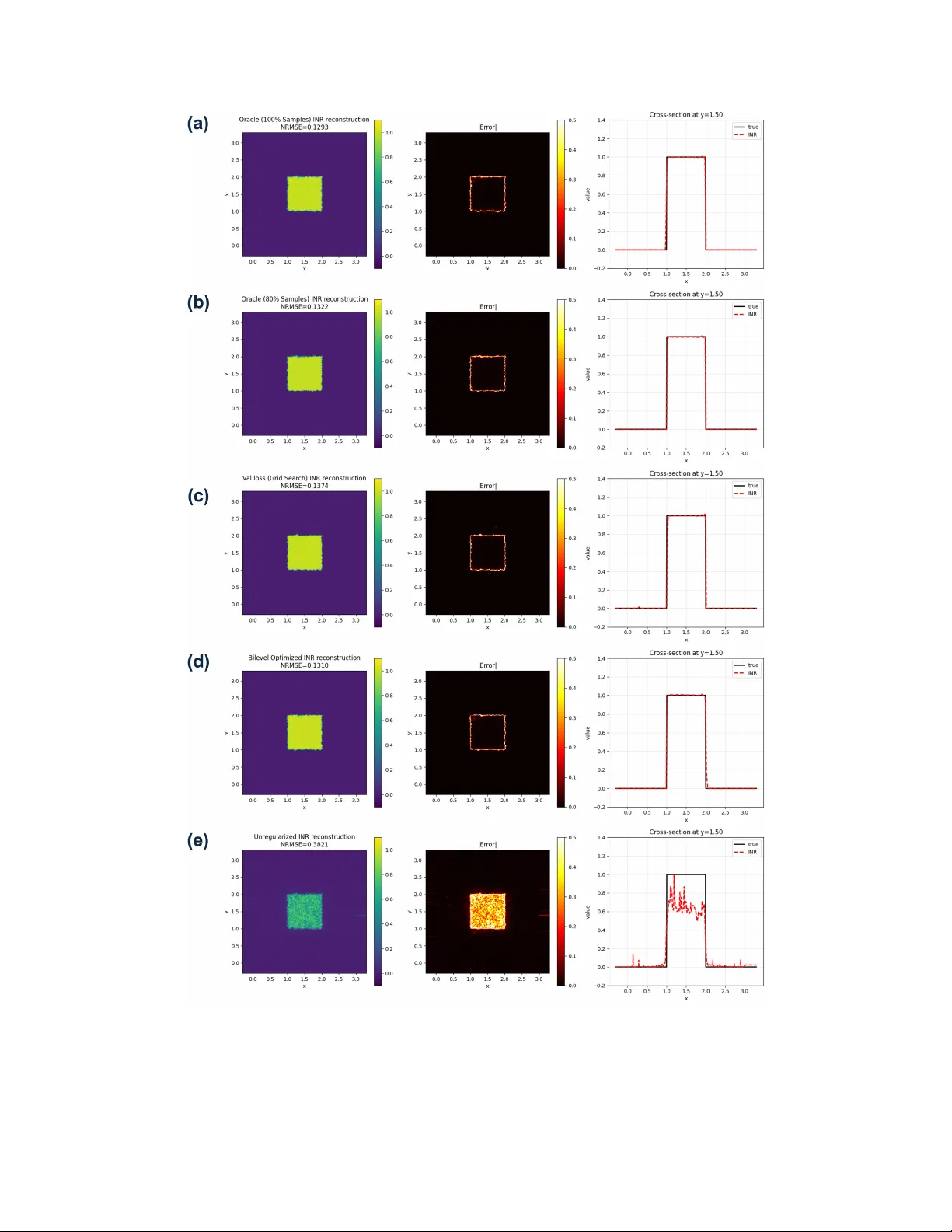
Comparing Implicit Neural Represen tations and B-Splines for Con tin uous F unction Fitting from Sparse Samples Hongze Y u 1 , Y un Jiang 2 , 3 , Jeffrey A. F essler 1 , 2 , 3 , 1 Departmen t of Electrical Engineering and Computer Science, Univ ersity of Mic higan 2 Departmen t of Biomedical Engineering, Universit y of Michigan 3 Departmen t of Radiology , Univ ersity of Michigan F ebruary 26, 2026 Abstract Con tinuous signal represen tations are naturally suited for inv erse problems, suc h as mag- netic resonance imaging (MRI) and computed tomograph y , because the measuremen ts dep end on an underlying physically contin uous signal. While classical metho ds rely on predefined ana- lytical bases lik e B-splines, implicit neural represen tations (INRs) hav e emerged as a pow erful alternativ e that use coordinate-based netw orks to parameterize contin uous functions with im- plicitly defined bases. Despite their empirical success, direct comparisons of their intrinsic represen tation capabilities with conv entional models remain limited. This preliminary empirical study compares a positional-enco ded INR with a cubic B-spline mo del for contin uous function fitting from sparse random samples, isolating the representation capacity difference by only using co efficien t-domain Tikhonov regularization. Results demonstrate that, under oracle hy- p erparameter selection, the INR achiev es a lo wer normalized ro ot-mean-squared error, yielding sharp er edge transitions and few er oscillatory artifacts than the oracle-tuned B-spline model. Additionally , w e sho w that a practical bilev el optimization framework for INR hyperparameter selection based on measurement data split effectiv ely approximates oracle performance. These findings empirically supp ort the sup erior represen tation capacity of INRs for sparse data fitting. 1 In tro duction Con tinuous signal represen tations mo del an unkno wn function f (  r ) using a parametric mapping f c (  r ), where the co efficien ts c are estimated from sampled data. The resulting function can be ev al- uated at arbitrary spatial locations. This approach is naturally suited for inv erse problems, such as magnetic resonance imaging (MRI) [1] and computed tomograph y , because the recorded measure- men ts (k-space samples in MRI and sinograms in tomograph y) depend on an underlying signal that is physically contin uous. Classical formulations typically use appro ximation spaces defined b y ana- lytical bases or kernels, including F ourier expansions, splines, and radial basis functions [2, 3, 4, 5]. Among these, B-splines are a common choice, where f (  r ) is represented in a finite-dimensional spline space defined by a set of knots. The knot density balances b et ween the approximation error and the noise sensitivit y . In practical applications, the sensing matrix deriv ed from basis functions is often ill-conditioned due to sparse sampling. A standard approac h is to regularize the inv erse problem with handcrafted smo othness- or sparsity-promoting p enalties. Recen t adv ances in computer graphics and computer vision, esp ecially in neural rendering and view syn thesis [6], hav e b oosted the developmen t of v arious contin uous signal representations. Ex- plicit mo dels construct scenes leveraging localized data structures or graphic primitives, such as 1 in terp olated feature grids [7] and 3D splats based on probabilit y distributions [8]. In con trast, implicit mo dels represents the signal as a contin uous, differen tiable function that can b e queried at arbitrary coordinates [9, 6, 10, 11, 12]. Among these, implicit neural representations (INRs) [13] ha ve emerged as a p o werful class of contin uous parametric models in whic h a multila y er p ercep- tron (MLP), comp osed with a p ositional enco der, maps spatial co ordinates  r directly to signal v alues. Unlik e the predefined analytical bases in con ven tional metho ds, the effective basis of an INR is implicitly defined b y the neural net w ork arc hitecture and its w eigh ts. INRs hav e b ecome increasingly p opular in MRI [14, 15, 16, 17, 18] in tasks suc h as undersampled reconstruction and sup er-resolution, where the con tinuous formulation aligns with the underlying physics of MRI. Despite their empirical success, few w orks ha v e directly compared con ven tional analytical meth- o ds (e.g., B-splines) and INRs in terms of their representation capabilities. T o address this gap and motiv ate the use of INRs, this pap er compares INRs with B-spline mo dels for contin uous function fitting from sparse, randomly sampled data. In this preliminary empirical study , b oth metho ds emplo yed Tikhono v regularization on their w eights or co efficients, pro viding a direct comparison of their intrinsic represen tation capacities, without confounding influence of additional handcrafted regularizers. F urthermore, w e in vestigate h yp erparameter selection in this function-fitting task. F or B-splines, we perform an oracle search (assuming access to ground truth) to determine the b est p ossible p erformance. F or INRs, we use a practical bilevel optimization approach [17], which relies on a train/v alidation split only .. The remaining materials are organized as follo ws. Section I I details the problem formulation and the compared metho ds. Section I I I describ es the exp erimen t settings. Sections IV and V presen t experiment results and discussions. 2 Metho ds 2.1 Problem F orm ulation Let f (  r ) : R d → R denote a con tinuous target function defined on a spatial domain. W e observ e N samples at random lo cations {  r n } N n =1 with corresponding v alues { y n } N n =1 , where y n = f (  r n ). The goal is to reco ver f on an arbitrary dense ev aluation grid ˜ z ∈ R N ev al × d from the measured v ector y = ( y 1 , . . . , y N ) T . 2.2 B-Spline F orm ulation As a metho d that is represen tative of typical predefined spatial basis functions using in solving in verse problems, w e in v estigated cubic B-splines with M uniformly spaced knots p er dimension, yielding M + 2 basis functions p er dimension and ( M + 2) 2 co efficien ts for the 2D function approx- imation using the standard tensor product represen tation: f c (  r ) = M +2 X i,j =1 c ij β (3)  r x − ξ i ∆  β (3)  r y − η j ∆  , (1) where ∆ is the knot spacing, and c ∈ R ( M +2) 2 denotes the v ectorized co efficien ts to b e computed from y . Hence, the Tikhono v regularized B-spline fitting is form ulated as: ˆ c ( λ ) = arg min c ∥ y − Φ c ∥ 2 2 + λ ∥ c ∥ 2 2 , (2) 2 where Φ is the design matrix (sensing matrix) of B-spline basis functions ev aluated at the sample lo cations. This quadratic cost function has a closed-form minimizer that we compute using Cholesky decomp osition ˆ c ( λ ) =  Φ ⊤ Φ + λ I  − 1 Φ ⊤ y . (3) 2.3 INR F orm ulation The INR parameterizes f as a comp osition of a p ositional enco der and an MLP deco der: f θ (  r ) = M θ MLP ( γ θ Enc (  r )) , (4) where γ θ Enc : R d → R K F is the m ultiresolution hash enco der with K levels and F features p er lev el, and M θ MLP : R K F → R is the MLP deco der. The netw ork weigh ts θ include b oth enco der weigh ts θ Enc and deco der weigh ts θ MLP . The weigh t-regularized INR fitting is formulated as: ˆ θ ( β ) = arg min θ 1 N ∥ y − f θ ( z ) ∥ 2 2 + λ Enc ∥ θ Enc ∥ 2 2 + λ MLP ∥ θ MLP ∥ 2 2 , (5) where z ∈ R N × d denotes the sample locations and y ∈ R N the corresponding observ ations. The h yp erparameter v ector β = ( λ Enc , λ MLP , τ , b ) includes the regularization strengths for the enco der and MLP w eigh ts, learning rate τ and the cross-level resolution scale factor b for the enco der. W e use Adam [19] to p erform the minimization in (5). 2.4 Oracle Hyp erparameter Searc h for B-Spline F or B-spline fitting, w e perform an oracle grid searc h o ver the regularization strength λ and n um b er of knots M , selecting the hyperparameters that minimize the normalized ro ot-mean-squared error (NRMSE) on the dense ev aluation grid ˜ z : λ ∗ , M ∗ = arg min λ,M   f ˆ c ( λ,M ) ( ˜ z ) − f true ( ˜ z )   2 ∥ f true ( ˜ z ) ∥ 2 . (6) This oracle searc h assumes access to the ground truth and serv es to b ound the ac hiev able perfor- mance. 2.5 Bilev el Optimization for INR In practice, the ground truth is una v ailable, and performing an oracle searc h for a m ultidimensional h yp erparameter vector can b e computationally inefficient. F ollowing the self-sup ervised h yp erpa- rameter optimization framew ork in [17], we split the observ ed samples in to a training set T and a v alidation set V , and p erformed bilevel optimization for INR: β ∗ = arg min β L V  ˆ θ ( β )  , s.t. ˆ θ ( β ) = arg min θ L T ( β , θ ) , (7) where L V  ˆ θ ( β )  = 1 |V | X n ∈V  y n − f ˆ θ ( β ) (  r n )  2 , (8) L T ( β , θ ) = 1 |T | X n ∈T  y n − f θ ( β ) (  r n )  2 + λ Enc ∥ θ Enc ∥ 2 2 + λ MLP ∥ θ MLP ∥ 2 2 , (9) 3 and β = ( λ Enc , λ MLP , τ , b ) includes regularization strengths, learning rate, and enco der scale factor. After computing β ∗ via bilevel optimization, we use the optimized β ∗ for one final round of function fitting using al l of the samples. 2.6 Oracle Analysis of INR Regularization T o in v estigate the sensitivity of INR to the weigh t decay hyperparameters, we p erformed an oracle grid search ov er λ Enc , λ MLP while fixing the learning rate τ and enco der scale factor b at their bilev el optimized v alues. The oracle optimal regularization strengths are: λ ∗ Enc , λ ∗ MLP = arg min λ Enc , λ MLP    f ˆ θ ( λ Enc , λ MLP ; τ , b ) ( ˜ z ) − f true ( ˜ z )    2 ∥ f true ( ˜ z ) ∥ 2 . (10) F or the v alidation loss based criterion, the optimal hyperparameters are selected b y minimizing the v alidation loss: λ ∗ Enc , λ ∗ MLP = arg min λ Enc , λ MLP L V  ˆ θ ( λ Enc , λ MLP ; τ , b )  . (11) W e compared four hyperparameter selection approac hes: (1) oracle NRMSE with grid searc h using 100% of samples for INR training, (2) oracle NRMSE with grid searc h using 80% of samples for training, (3) v alidation loss with grid searc h using an 80%/20% train/v alidation split, and (4) v alidation loss with Ba y esian optimization (bilev el optimization) [17]. 2.7 Ev aluation Metric F or b oth metho ds, w e rep ort the NRMSE on the ev aluation grid: NRMSE( ˆ f ) = ∥ ˆ f ( ˜ z ) − f true ( ˜ z ) ∥ 2 ∥ f true ( ˜ z ) ∥ 2 , (12) where ˆ f denotes the reconstructed function ( f ˆ c or f ˆ θ ). 3 Exp erimen ts T o compare the representation capacit y of INR and B-spline, w e fit a 2D rect function: f ( x, y ) = Rect  x − 3 2  Rect  y − 3 2  , (13) using N = 10000 p oin ts sampled uniformly at random on [0 , 3] × [0 , 3]. Both metho ds are ev aluated on a dense 501 × 501 uniform grid ˜ z cov ering [ − 0 . 3 , 3 . 3] × [ − 0 . 3 , 3 . 3]. Only Tikhono v regulariza- tion on w eights/coefficients is applied, excluding additional handcrafted regularizers to isolate the represen tation capacit y of eac h mo del. F or B-spline fitting, we used cubic B-splines with uniformly spaced knots and p erformed an oracle grid search o ver the regularization strength log 10 λ ∈ [ − 5 , 5] with step size 0.1 (101 v alues), and the n um b er of knots M ∈ { 5 , 10 , 15 , . . . , 100 } (20 v alues). F or INR, we used the hash-encoded architecture described in [17] with an 80%/20% train/v alidation split. The bilev el optimization ran 60 upp er-lev el iterations with 2,000 lo w er-level iterations eac h to obtain the optimized hyperparameter vector β ∗ . F or the hyperparameter sensitivity analysis, w e fixed the learning rate τ and enco der scale factor b at their bilev el optimized v alues and p erformed 4 grid searches o v er log 10 λ Enc ∈ [ − 4 , − 1] and log 10 λ MLP ∈ [ − 9 , − 6] matching the bilevel optimiza- tion range, eac h with step size 0.1 (31 v alues p er axis). The grid search was conducted using three selection criteria: oracle NRMSE with 100% training samples, oracle NRMSE with 80% training samples, and v alidation loss with 80%/20% train/v alidation split. 4 Results 4.1 B-Spline Results Figure 1: Cubic B-spline fitting with oracle grid search ov er regularization strength λ and n um b er of knots M . T op row: NRMSE heatmap showing the optimal at M = 75, λ = 2 . 51 × 10 − 2 (red star); NRMSE v ersus λ for different M ; NRMSE v ersus M for differen t λ . Bottom ro w: optimal reconstruction, absolute error map, and cross-section at y = 1 . 50. The optimal NRMSE is 0.1540. Fig. 1 shows the B-spline fitting results with oracle grid searc h ov er Tikhonov regularization strength λ and num ber of knots M . The optimal h yp erparameter set achiev ed NRMSE = 0 . 154 at M ∗ = 75 and λ ∗ = 2 . 51 × 10 − 2 . The NRMSE heatmap (top left) and NRMSE vs λ plot (top middle) reveal three differen t regimes dep ending on M . F or M < 50, the B-spline mo del underfits the data and Tikhonov regularization pro vides no improv emen t. F or M ∈ [50 , 80), regularization near λ = 10 − 2 reduces NRMSE compared to the unregularized case (e.g., by 0.09 for M = 75). F or M ≥ 80, the model o verfits. While regularization helps, the minimum NRMSE remains higher than the optimal at M = 75. The NRMSE versus M curv es (top righ t) further shows that λ ≈ 10 − 2 consisten tly 5 Figure 2: Effect of Tikhonov regularization on cubic B-spline fitting with M = 75 knots. (a) T rue function with random samples. (b) Unregularized fit sho wing oscillatory artifacts. (c) Optimally regularized fit ( λ = 0 . 0251) with reduced artifacts but increased blur. (d) NRMSE versus λ , illustrating the bias-v ariance tradeoff. pro duces the low est error across differen t knot counts. Ev en for the setting that achiev ed the lo w est NRMSE, the optimized B-spline reconstruction (b ottom ro w) exhibits noticeable artifacts near the discon tinuities and residual oscillations in the flat-top region, as sho wn in the cross-section at y = 1 . 50. Fig. 2 compares the unregularized and optimally regularized B-spline fits at M = 75. The unregularized fit (b) shows pronounced oscillatory artifacts near the rectangle edges due to o ver- fitting. Tikhonov regularization (c) suppresses these artifacts but in tro duces visible blurring. The NRMSE curve (d) shows a general trend of Tikhono v regularization in B-spline fitting: insufficien t regularization ( λ < 10 − 3 ) results in o v erfitting, whereas excessiv e regularization ( λ > 10 0 ) causes o ver-smoothing. 4.2 INR Results Fig. 3 sho ws the INR hyperparameter sensitivit y analysis ov er the enco der and MLP weigh t deca y parameters ( λ Enc , λ MLP ). The oracle NRMSE heatmap with 100% training samples (a) yields the optimal w eigh t decay pair ( λ Enc , λ MLP ) = (7 . 94 × 10 − 3 , 1 . 00 × 10 − 6 ). Using 80% training samples 6 Figure 3: INR h yp erparameter sensitivity analysis ov er enco der and MLP weigh t decay ( λ Enc , λ MLP ). (a) Oracle NRMSE with 100% training samples. (b) Oracle NRMSE with 80% training samples. (c) V alidation loss with 80%/20% train/v alidation split. Mark ers indicate optima: cyan triangle (100% oracle), magenta square (80% oracle), red star (v alidation grid searc h), yello w diamond (Bay esOpt). (b) pro duces a similar optim um at (1 . 00 × 10 − 2 , 7 . 94 × 10 − 7 ), indicating that the reduced training set has only a mo dest effect on the optimal h yp erparameters in this task. When using v alidation loss as the selection criterion with grid searc h (c), the optim um shifts to (1 . 26 × 10 − 2 , 5 . 01 × 10 − 7 ), which is further from the oracle solution. Ho wev er, the bilevel optimization scheme using Ba yesian optimization (Ba yesOpt) finds a sup erior solution at (7 . 55 × 10 − 3 , 9 . 87 × 10 − 7 ), closely approximating the oracle optim um despite having no access to the ground truth and limited iterations (60 upper-level iterations compared to 961 grid searc h ev aluations). Fig. 4 compares INR reconstructions under differen t hyperparameter selection strategies. Among the four regularized approac hes (a–d), oracle grid searc h with 100% samples ac hieved the low est NRMSE of 0.129, represen ting the b est achiev able p erformance. The bilevel optimized INR (d) ac hieves NRMSE = 0 . 131, closely matching the oracle and outperforming b oth the 80% oracle grid searc h (NRMSE = 0 . 132) and the v alidation loss grid searc h (NRMSE = 0 . 137). Notably , all four regularized INR results outp erformed the optimal B-spline result (NRMSE = 0 . 154). Visually , all regularized INR reconstructions exhibit minimal artifacts in the flat-top region of the rectangle, with residual errors mainly app earing near the discon tinuities. The cross-section plots at y = 1 . 50 confirm sharp er edge transitions and reduced ringing compared to the B-spline results in Fig. 1. The unregularized INR result in Fig. 4 demonstrates the critical importance of w eight regular- ization for INR. Despite ac hieving near-zero training loss, the ov erparameterized nonlinear mo del sev erely ov erfits without regularization, resulting in NRMSE = 0 . 3821 with pronounced artifacts: underestimation within the rectangle region and spurious oscillations elsewhere. This confirms that, without prop er regularization, the expressive capacity of hash-enco ded INR leads to p o or generalization from sparse samples. 5 Discussion and Conclusions This work presen ts preliminary exp erimen ts comparing INR and finite-series B-spline representa- tions for contin uous function fitting from sparse random samples. Both metho ds used only Tikhono v regularization on their resp ectiv e weigh ts/co efficien ts, isolating the comparison to representation capacit y without additional handcrafted priors. 7 5.1 Comparison of Represen tation Capacity The results demonstrate that, under oracle h yp erparameter selection, the hash-enco ded INR (NRMSE = 0 . 129) outp erformed the cubic B-spline (NRMSE = 0 . 154) for fitting a 2D rect function. The INR reconstructions exhibited sharper edge transitions and few er oscillatory artifacts in the flat-top region compared to B-spline, as sho wn in the cross-section plots. Ho wev er, the improv ed p erformance comes with tradeoffs. The INR con tains substantially more parameters than the B-spline mo del, making it less parameter-efficien t. Additionally , the B- spline form ulation is more in terpretable, and its NRMSE heatmap is also smo other than the INR heatmaps. The “rougher” INR landscap e ma y be due to the random small w eight initialization used for each fit, whic h in tro duces the only source of sto c hasticit y in this toy exp erimen t. By contrast, in the MRI reconstruction exp eriments [17], rep eated runs with different initializations pro duced nearly iden tical reconstructions, suggesting that weigh t initialization has a smaller practical impact in that setting. A more thorough theoretical analysis of INR represen tation and its implicit biases remains an activ e research direction. 5.2 Effect of Tikhono v Regularization Both metho ds b enefit from Tikhono v regularization, but the effect differs due to their mo del dif- ferences. F or B-spline fitting, regularization directly penalizes co efficien t magnitudes, introducing a bias-v ariance tradeoff where reduced oscillations come at the cost of increased blurring (Fig. 2). F or INR, the enco der-deco der architecture enables a differen t regularization scheme. W eight p enalt y on the enco der ( λ Enc ) directly regularizes the m ultiresolution feature representation, while the smaller MLP regularization ( λ MLP ) only mildly constrains the deco ded contin uous function. The final linear lay er can rescale outputs, partially comp ensating for magnitude shrink age from regularization of the enco der. This, combined with the muc h richer nonlinear function class provided b y the ov erparameterized mo del, may explain why INR achiev ed low er NRMSE with Tikhonov regularization alone, without requiring additional image-domain priors. The unregularized INR result (NRMSE = 0 . 382) further emphasizes the imp ortance of regular- ization for the o verparameterized hash-encoded architecture. Without w eight regularization, the mo del o verfit sev erely despite ac hieving near-zero training loss. 5.3 Efficacy of Bilev el Optimization The hyperparameter sensitivity analysis demonstrates that bilevel optimization using Bay esian optimization can effectiv ely approximate oracle performance like the accelerated MRI reconstruc- tion task. The bilevel optimized INR (NRMSE = 0 . 131) closely matched the 100% oracle result (NRMSE = 0 . 129) and outperformed v alidation-based grid searc h (NRMSE = 0 . 137), despite op- erating in con tinuous hyperparameter space with only 60 upp er-lev el iterations compared to 961 grid search ev aluations. This result supp orts the use of bilevel optimization for automatic h yp erparameter selection when ground truth is unav ailable, as is the case in practical MRI reconstruction. 5.4 Conclusions In summary , this preliminary study pro vides empirical evidence that hash-enco ded INR with Tikhono v regularization can outp erform cubic B-spline for fitting discon tinuous functions from sparse samples, and that bilevel optimization can effectiv ely select near-optimal hyperparameters without ground truth access. F urther study on extending the exp eriments to more complex tasks, 8 suc h as realistic MR reconstruction settings, remains a future direction. It w ould also be interesting to inv estigate fitting a smooth function that can be represen ted p erfectly b y cubic B-splines. Ac kno wledgmen t This study w as supp orted in part b y NIH gran ts R37CA263583, R01CA284172, Siemens Healthi- neers and Cook Medical. References [1] J. A. F essler, “Model-based image reconstruction for MRI,” IEEE Signal Pr o c ess. Mag. , v ol. 27, no. 4, pp. 81–89, 2010. [2] G. W ahba, Spline Mo dels for Observational Data . SIAM, 1990. [3] M. Unser, “Splines: a p erfect fit for signal and image pro cessing,” IEEE Signal Pr o c ess. Mag. , v ol. 16, no. 6, pp. 22–38, 1999. [4] S. Mallat, A wavelet tour of signal pr o c essing . Academic Press, 1999. [5] H. W endland, Sc atter e d Data Appr oximation . Cambridge: Cambridge Univ ersity Press, 2005, v ol. 17. [6] B. Mildenhall, P . P . Sriniv asan, M. T ancik, J. T. Barron, R. Ramamoorthi, and R. Ng, “NeRF: Represen ting scenes as neural radiance fields for view synthesis,” in Pr o c. ECCV , 2020. [7] S. F rido vich-Keil, A. Y u, M. T ancik, Q. Chen, B. Rech t, and A. Kanaza wa, “Pleno xels: Radi- ance fields without neural netw orks,” in Pr o c. CVPR , 2022, pp. 5501–5510. [8] B. Kerbl, G. Kopanas, T. Leimk¨ uhler, and G. Drettakis, “3D Gaussian Splatting for Real-Time Radiance Field Rendering,” ACM T r ans. Gr aphics , v ol. 42, no. 4, July 2023. [Online]. Av ailable: https://repo- sam.inria.fr/fungraph/3d- gaussian- splatting/ [9] J. J. P ark, P . Florence, J. Straub, R. Newcom b e, and S. Lov egrov e, “DeepSDF: Learning con tinuous signed distance functions for shap e represen tation,” in Pr o c. CVPR , 2019, pp. 165–174. [10] J. T. Barron, B. Mildenhall, M. T ancik, P . Hedman, R. Martin-Brualla, and P . P . Sriniv asan, “Mip-NeRF: A m ultiscale represen tation for anti-aliasing neural radiance fields,” ICCV , 2021. [11] T. M ¨ uller, A. Ev ans, C. Sc hied, and A. Keller, “Instant neural graphics primitives with a m ultiresolution hash enco ding,” A CM T r ans. Gr aph. , v ol. 41, no. 4, pp. 102:1–102:15, Jul. 2022. [12] M. T ancik, P . P . Sriniv asan, B. Mildenhall, S. F rido vich-Keil, N. Raghav an, U. Singhal, R. Ra- mamo orthi, J. T. Barron, and R. Ng, “F ourier features let net works learn high frequency functions in lo w dimensional domains,” in Pr o c. NIPS , 2020. [13] V. Sitzmann, J. N. Martel, A. W. Bergman, D. B. Lindell, and G. W etzstein, “Implicit neural represen tations with p eriodic activ ation functions,” in Pr o c. NIPS , 2020. 9 [14] L. Shen, J. Pauly , and L. Xing, “NeRP: Implicit neural represen tation learning with prior em b edding for sparsely sampled image reconstruction,” IEEE T r ans. Neur al Netw. and L e arn. Syst. , vol. 35, no. 1, pp. 770–782, 2024. [15] R. F eng, Q. W u, J. F eng, H. She, C. Liu, Y. Zhang, and H. W ei, “IMJENSE: Scan-sp ecific implicit represen tation for join t coil sensitivity and image estimation in parallel MRI,” IEEE T r ans. on Me d. Imag. , v ol. 43, no. 4, pp. 1539–1553, 2024. [16] J. F eng, R. F eng, Q. W u, X. Shen, L. Chen, X. Li, L. F eng, J. Chen, Z. Zhang, C. Liu, Y. Zhang, and H. W ei, “Spatiotemp oral implicit neural representation for unsup ervised dynamic MRI reconstruction,” IEEE T r ans. Me d. Imag. , pp. 1–1, 2025. [17] H. Y u, J. A. F essler, and Y. Jiang, “Bilev el optimized implicit neural representation for scan-sp ecific accelerated mri reconstruction,” 2025. [Online]. Av ailable: h ttps: [18] J. Lyu, L. Ning, W. Consagra, Q. Liu, R. J. Rushmore, B. Bilgic, and Y. Rathi, “Rapid whole brain motion-robust mesoscale in-viv o MR imaging using multi-scale implicit neural represen tation,” Me d. Imag. Analysis , v ol. 107, p. 103830, 2026. [19] D. P . Kingma and J. Ba, “Adam: A metho d for sto chastic optimization,” 2017. [Online]. Av ailable: 10 Figure 4: INR reconstruction results under differen t h yp erparameter selection criteria. Each ro w sho ws the reconstruction, absolute error map, and cross-section at y = 1 . 50. (a) Oracle grid search with 100% samples (NRMSE = 0 . 129). (b) Oracle grid search with 80% samples (NRMSE = 0 . 132). (c) V alidation loss grid search with 80%/20% split (NRMSE = 0 . 137). (d) Bilev el optimization with 80%/20% split (NRMSE = 0 . 131). (e) Unregularized fitting (NRMSE = 0 . 382). 11