Robustness certificates in data-driven non-convex optimization with additively-uncertain constraints

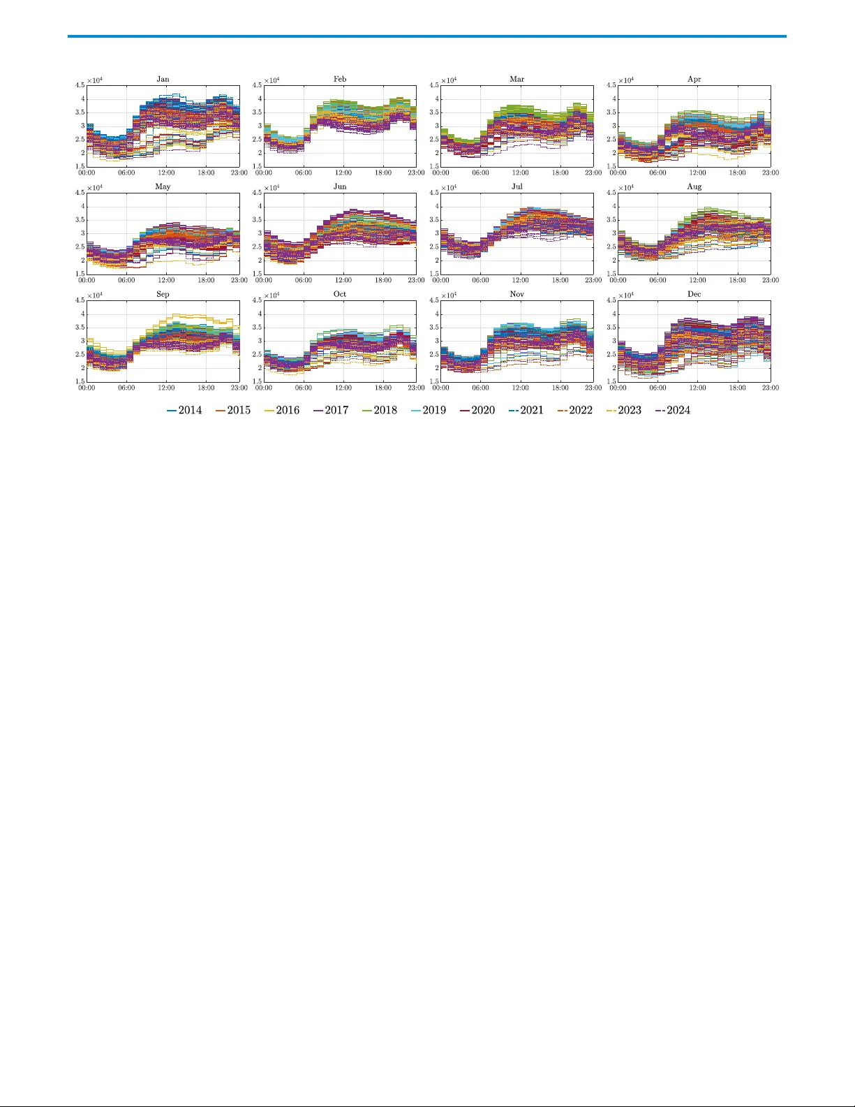
1 Rob ustness cer tificates in da ta-dr iv en non-con v e x optimization with additiv ely-unc er tain c onstr aints Ale xander J . Gallo Membe r , IEEE , Massimiliano Zogg ia, Alessa ndro F alsone Member , IEEE , Maria Prandini Fello w , IEEE , and Simone Gar atti Memb er , IEEE Abstract — W e consid er decisi on-making problems that are formulated a s non-convex op timization programs where uncer tainty enters the con straints through an additive t erm, indepe ndent of the decisio n variables, and robustness is imposed us ing a fi nite data -set, according to the scena rio robust op timization pa radigm. By exploit ing the structure of the constra i nts, we s how that both a priori an d a posteri ori distribution- free probabilistic robustness cer tifica tes for a possibly sub-opti mal solu tion to th e re s ulting data-driv en optimization pr oblem can be obtaine d with minimal compu- tational effor t. Buildin g on these resul ts, we also dis cuss a one-sho t and a n i ncrementa l procedure to determine the siz e of the data-se t so a s to gua rantee a user-chosen robustness level. Nota bly , both the a posteriori robustness asses sment and incremental data -set sizing do no t require to solve the no n -convex scenario program. A comparative analysis performed on the un it commitment problem using real data reveals a li mited i ncreas e in con ser vati venes s with a sig nifican t computati onal savin g with respe c t to the appli cation of sce nario theor y results for gen eral, non neces sarily struc tured, non-con vex p roblems. I . I N T R O D U C T I O N In this p a per we con sid e r design prob lems where decisions are taken in the presen ce of un certainty that is known from data. W e focus on the case when the decision-ma king problem is form u lated as a d ata-driven optimization progr a m of the following f orm min x ∈X f ( x ) (1) s.t. h ( x, δ i ) ≤ 0 , i = 1 , . . . , N , P aper par tly suppor ted by F AIR (F u ture Ar tificial Intelligen ce Re- search) project, funded by the NextGener ationEU program within the PNRR-PE-AI scheme (M4C2, Inv estment 1.3, Line on Ar tificial Intelli- gence), by the PRIN PNRR project P2022NB77E “A data-driven coop- erativ e frame work f or the management of d i stributed energy and water resources” (CUP: D53D23016100001), funded by the NextGeneration EU progr am (Mission 4, Component 2, Inv estment 1.1), by the PRIN 2022 project “The Scenario Approach f or Control and Non-Conv ex Design” (project number D53D23001450006), and by the Italian Ministr y of Enter prises and Made in Italy i n the frame work of the project 4DDS (4D Drone Swarms) under g rant no . F/310097/01-04/X56. The authors are with the Dipar timento di Elettronica Inf or- mazione e Bioingegneria, P ol itecnico di Milano , Piazza Leonardo da Vinci 32, 20133 Milano, Italy (e-mail: alexanderjulian.gallo , alessandro .f alsone, maria.prandini, simone.garatt i@polimi.it; massimil- iano .zoggia@mail.polimi.it). where x is the decision variable an d ( δ 1 , δ 2 , . . . , δ N ) is the data-set represen ting a vailable instances of th e u ncertainty δ taking values in some set ∆ . Set X ⊆ R d may encod e integer constraints, e.g., when it is a subset of R n c × { 0 , 1 } n d with n c + n d = d . The scalar-v alued function f ( · ) : X → R is the cost to be min imized, while the q -dimen sional function h ( · , · ) : X × ∆ → R q depend s on b oth x and the un certainty δ and defin e s the constrain ts o f the problem. In (1), constraints are imposed f or all available d ata to try to enforce ro bustness against uncertainty . Th e solution of the co nstrained optimiz a - tion p rogram (1) depend s o n th e d ata-set ( δ 1 , . . . , δ N ) an d is denoted with th e shorth and x ⋆ N for ease of refer ence. The scenario appr o ach [1] –[3] ad dresses the issue of evalu- ating th e r obustness o f the decision x ⋆ N by a ssessing th e risk that it vio lates un seen instances (“scenario s”) of the uncer- tainty δ , which is modeled as a rando m ou tcome fro m some underly ing ( ty pically unkn own) pr obability space (∆ , D , P ) . Theoretical [4]–[ 11] a s well as application- oriented [1 2]– [16] results ha ve been d eveloped within th e scenario fr a me- work. In the earliest theoretical finding s in the context o f conv ex ro bust optimization [4], risk is assessed a priori , in terms of a n upper boun d guaran teed w ith a certain confiden ce and associated with the nu m ber N o f scenarios. More recently , it was sh own that tigh ter risk assessments can be o btained by means o f a p osteriori computed upper b ounds [8], [17], depend ing o n the o ptimal solution x ⋆ N and the collected data. This theo r y ap plies also to n on-co n vex op timization problem s and various other decision schemes [11], [18], for which equiv alent a p rio ri bo unds either d o no t exist (fo r gen eral problem s) or are very conservativ e (for specific proble m s, e.g., [19], [20 ]). In this paper , we consid e r scenario optim ization prog rams of the form min x ∈X f ( x ) (2) s.t. g ( x ) ≤ b ( δ i ) , i = 1 , . . . , N , where the constraint fu n ction has the following structure: h ( x, δ ) = g ( x ) − b ( δ ) , with g : X → R q and b : ∆ → R q depend ing o nly on the decision variable x an d the u ncertainty δ , respectively . This kind of problem s ap p ears in a variety of decision makin g settings, includin g model pr edictive control for lin e ar systems with additive distur bances [21 ] , [22], p o s- 2 sibly in the p resence of quantized in puts, as well as prob lems in energy managem ent, such as u nit commitme nt [23] a n d econom ic dispatch [24]. In this paper, we explore h ow th e separable structure of the constraints can be exp lo ited to pr ovide the decision maker with a set o f to ols for risk assessment that is wider th an those that are a vailable fo r general, n ot necessarily stru ctured non-conve x problem s. In particular , easy-to- compu te ro bustness certificates can be provided for any p ossibly sub-o ptimal solution o f the scenario prog ram, and no t only fo r the optimal one. As such, they are relev ant in tho se (n on-co n vex) setting s whe re the solution is har d to compu te , e.g., becau se o f the pre sence of local minima or the combin atorial nature of the pr oblem. Specifically , we show that i. the risk o f any feasible solu tion to (2 ) is upper boun ded by the risk of an associated, c onv ex, scena r io problem; ii. a po steriori robustness certificates on any possibly sub - optimal scenario so lution can be co mputed with minim al computatio nal effort, withou t solving the scenario op ti- mization pr oblem; iii. a priori risk assessment can b e per f ormed and used for data-set sizing; iv . the num ber of scen arios needed to compute a possibly sub-optim al scenar io solution with a certain a priori guar- anteed r obustness lev el can b e red uced using an iterativ e proced u re where the d ata-set size is g rown p r ogressively and the o ptimization prob lem is so lved only at the final iteration. Our results are demonstra te d on the unit commitment problem, which co nsists in determining which generators in a poo l should be turne d on/off an d how much p ower they should produ ce over a given time h orizon to mee t the electr icity demand at th e lowest cost. Using real-world data, our results show a limited increase in con servati veness, while p roviding substantial computatio nal advantages in evaluating r o bustness guaran tee s, co mpared to stand ard scenario th eory . Some resu lts on improved r obustness g uarantees on the scenario solution th a t exp lo it the structure of th e constraints in the scen a r io prog ram are a lso av ailable in [25], [26 ]. Howe ver, they are confin ed to the conve x case and they provid e on ly a priori robustness guar a ntees for one-sh ot sizing of th e data-set based on [4]. A p r eliminary version o f this work was presented in [27]. This paper dif fers from [ 2 7] in th at here we co nsider the risk of any feasible solution to the non -conve x scenario program and make exp licit tha t it is u pper bo unded by the r isk of a con vex progr am, so that tighter results fro m [4] can b e leveraged. Furthermo re, while in [27] we pr esented a simple ar tificial numerical example, here we show the effectiv eness of our method when app lied to the mo re co mplex u nit commitmen t problem u sing real d ata o f the hourly agg regate load demand from the Span ish transmission system oper ator (TSO) Red El ´ ectrica. The remain der o f this paper ha s th e following structu r e. In Section II, we provide a br ief sum mary of the f undam ental concepts of the scena r io app roach that are relev ant to the present work. Referen ce is mad e to the da ta - driven o ptimiza- tion pro blem (1) to th en show how these general r esults can b e exploited in the structu red case (2). Specifically , in Sec tion II I we sh ow that the risk of co nstraint v iolation associated to a ny feasible solution to (2) is up per boun ded by that of the op timal solution of a simp ler , conv ex scenario pro blem. T his result is then explo ited to provide easily-co m putable distribution-free probab ilistic robustness ce rtificates. Data-set sizing to a c hieve solutions with a user-defined robustness le vel is discussed in Section IV. Fina lly , the effectiveness of the pro posed appro ach is dem onstrated on the un it commitm ent problem using real data in Section V. Som e c oncludin g remark s are g iv en in Section VI. I I . R E L E VA N T R E S U L T S F R O M S C E N A R I O T H E O R Y Consider a scenar io progra m of the form (1) where ( δ 1 , . . . , δ N ) is a data-set of N uncertainty realizations called “ scen arios” and mo deled as ind ependen t draws from (∆ , D , P ) . The f ollowing assum ptions are in ord er . Assumption 1: The scen ario pro blem (1) is feasible with probab ility on e , for every N . ⊳ Assumption 2: The scenario pro blem (1 ) admits a un ique optimal solutio n x ⋆ N with prob ability one, for every N . ⊳ W ith r eference to (1) , a de cision x ∈ X i s said to be inappr opria te for the u n certainty realization δ ∈ ∆ if th e constraint in (1) is n ot satisfied f or that δ . W e can then define the risk associated to a decision x ∈ X as the vio lation probab ility V ( x ) = P { δ ∈ ∆ : h ( x, δ ) 6≤ 0 } , (3) which is the probab ility measu re of the set of uncerta in ty realizations fo r which x is inappr opriate. The risk V ( x ⋆ N ) associated with the o ptimal solution x ⋆ N to (1) is a rando m quantity since it depends on x ⋆ N , which is a ran dom variable defined on the product pr obability space (∆ N , D ⊗ N , P N ) . The scenario theory allows to determin e a bound on V ( x ⋆ N ) that h o lds with a certain confiden ce. Suc h a bound is distrib ution -free, in that it is valid irrespec ti vely o f the under lying proba bility P , an d it depends on an ob serva ble quantity called comp lexity , [1 1]. Instrumen tal to the defin ition of comp lexity is that of support list . Definition 1 (Supp ort list): Given a list of scenar ios ( δ 1 , . . . , δ N ) , a sup p ort list of the scenario p r ogram (1) is any sub-list of length k ∈ { 0 , 1 , . . . , N } , S k N = ( δ i 1 , . . . , δ i k ) , with i 1 < i 2 < · · · < i k such that: i. x ⋆ S k N = x ⋆ N , where x ⋆ S k N is the minimizer o f (1) with scenarios in S k N only . ii. S k N is irr educible, i.e., no elem ent can be r emoved f rom S k N without cha n ging the solutio n to (1 ). ⊳ Definition 2 (Complexity): For any given data-set ( δ 1 , . . . , δ N ) , the complexity s ⋆ N of the associated scen a rio progr am (1 ) is the size of th e smallest sup port list. 1 ⊳ A fu ndamen tal result in [11] is gi ven by th e following theorem, rep hrased according to o ur notatio n. Theor em 1 ( Theor em 6 in [11]): Un der Assumptio ns 1 and 2, for any confidence lev el β ∈ (0 , 1) , the risk V ( x ⋆ N ) of 1 The comple xity s ⋆ N is a function of the scenarios ( δ 1 , . . . , δ N ) but this depende nce is not made explic it for ease of notati on. 3 the o p timal solution to (1) satisfies P N { V ( x ⋆ N ) ≤ ǫ N ,β ( s ⋆ N ) } ≥ 1 − β , (4) where th e violation function ǫ N ,β : { 0 , 1 , . . . , N } → [0 , 1] is defined as ǫ N ,β ( k ) = ( 1 − t ( k ) , k = 0 , 1 , . . . , N − 1 1 , k = N (5) with t ( k ) being th e uniqu e so lu tion in [0 , 1] to β N N − 1 X m = k  m k  t m − k −  N k  t N − k = 0 . (6)  Equation (6) c a n be efficiently so lved b y b isection; co nse- quently , e valuating ǫ N ,β for a gi ven k is compu tationally cheap (see Append ix B.1 in [ 1 8] for a r eady-to- use MA TLAB code). Note tha t we inclu de both N and β in the notation of the fun ction ǫ N ,β ( · ) to h ighlight that its definition d epends explicitly on the num b er of scen arios in (1), an d the desired confidenc e. Observe that the probab ility appearin g in (4) is P N since the ran dom qu antities x ⋆ N and s ⋆ N that are inv olved d e p end on the N i.i.d . scenario s ( δ 1 , . . . , δ N ) and are hence defin ed on the prod uct prob ability spac e (∆ N , D ⊗ N , P N ) . Ine q uality (4) means that there is a pr obability o f at least 1 − β that the data- set drawn from ∆ N is such that its associated co mplexity s ⋆ N leads to a value of ǫ N ,β ( s ⋆ N ) fo r which the bou nd V ( x ⋆ N ) ≤ ǫ N ,β ( s ⋆ N ) h olds. Thus, ǫ N ,β ( s ⋆ N ) is the robustness level of the optimal solutio n to the scenario pro g ram (1), which is guaran tee d with confidence 1 − β . Function ǫ N ,β ( · ) is non- decreasing so that ( as expected) th e higher the complexity is, the weaker the ro bustness guarantees are, in terms o f bound on the risk. A few remarks are in order to highligh t some challenges in applying these results to a non-co n vex settings. Firstly , they refer to the op timal solution, which may b e h ard to comp ute. Secondly , comp uting the minimal supp o rt list may be a very hard com binatorial prob lem. While useful guar antees can still be o btained by identif ying any supp ort list (not n ecessarily minimal, because function ǫ N ,β ( · ) is non-decrea sin g ), this can remain com putation a lly challeng ing. I ndeed, while in the conv ex case it is often the case that a suppo rt list is alm o st surely d etermined b y those constraints that are active at the solution (i.e . , it is form ed by th e δ i ’ s such that h ℓ ( x ⋆ N , δ i ) = 0 , for some ℓ ∈ { 1 , . . . , q } , wh ere h ℓ denotes the ℓ -th compon ent of the constraint function h in (1)), for non-co n vex scenar io problem s scen a rios resultin g in non-a c tive con straints may be part o f suppor t lists. Thus, finding a support list may req uire removing scen arios one by on e and repeated ly solv ing the n on- conv ex p rogram . Finally , there is in g eneral no a priori bo und on s ⋆ N , which may be as large a s N . This pr ev ents on e to a priori determine a sufficiently large data-set size guaran teeing that th e resulting risk V ( x ⋆ N ) do es not exceed a u ser-chosen threshold with high confide n ce. I I I . R O B U S T N E S S C E R T I FI C A T E S F O R N O N - C O N V E X S C E N A R I O P R O B L E M S W I T H A D D I T I V E L Y - U N C E R TAI N C O N S T R A I N T S This section pr esents the theo r etical con tributions of the paper . W e start by showing th at the risk of the n on-co nvex scenario pr o blem in (2 ) can b e up per bou nded b y the r isk of a suitably defin e d conv ex scena r io prob lem, f or any data- set of scenarios, a n d any p robability sp a ce (∆ , D , P ) . Based on this result, we derive a posteriori an d a priori risk certificates for problem (2 ). Suppose th a t th e additively-uncertain scen ario progra m (2 ) satisfies the feasibility Assum ption 1 an d let ˆ x ⋆ N ∈ X deno te a p ossibly sub -optimal yet feasible solution (e.g ., ob tained by a n umerical solver that ensures feasibility but not optimality). Consider the f ollowing co n vex scenario progr a m max ξ ∈ R q q X ℓ =1 ξ ℓ (7) s.t. ξ ℓ ≤ b ℓ ( δ i ) , ℓ = 1 , . . . , q , i = 1 , . . . , N , where b ℓ ( · ) is the ℓ -th com p onent of the fun c tion b ( · ) ap - pearing in th e co nstraints of (2). The linea r prog r am (7) is always feasible and h as a u nique solu tio n given by ξ ⋆ N = [ ξ ⋆ N , 1 . . . ξ ⋆ N ,q ] ⊤ , where ξ ⋆ N ,ℓ = min i =1 ,...,N b ℓ ( δ i ) , ℓ = 1 , . . . , q . (8) Denote with V ′ ( ξ ⋆ N ) the risk associated to the so lution ξ ⋆ N of the scenario program (7): V ′ ( ξ ⋆ N ) = P { δ ∈ ∆ : ξ ⋆ N 6≤ b ( δ ) } . W e can now state our first result. Theor em 2: Con sider the scenario pro grams (2) and (7) associated to the sam e data-set ( δ 1 , . . . , δ N ) of scen arios drawn independen tly fro m (∆ , D , P ) . For any proba bility P , for any data- set ( δ 1 , . . . , δ N ) , the risk of a possibly sub- optimal so lu tion ˆ x ⋆ N of the scena rio pr ogram (2 ) is up per bound ed by the risk of the o ptimal solution ξ ⋆ N of th e scenario progr am (7 ), i.e., V ( ˆ x ⋆ N ) ≤ V ′ ( ξ ⋆ N ) . (9) Pr oof: For each ℓ = 1 , . . . , q , the co nstraints g ℓ ( x ) ≤ b ℓ ( δ i ) , i = 1 , . . . , N , in (2 ) are nested and domin ated b y th e one with the smallest b ℓ ( δ i ) . Thus, the optimal solution ξ ⋆ N to the linear program (7) giv en in (8) defines the whole feasibility region of ( 2), by using g ( x ) ≤ ξ ⋆ N in place of its c o nstraints. It ther e f ore fo llows that g ℓ ( ˆ x ⋆ N ) ≤ ξ ⋆ N ,ℓ is satisfied for all ℓ = 1 , . . . , q . Because of this, for any δ ∈ ∆ , the fo llowing implication hold s g ℓ ( ˆ x ⋆ N ) > b ℓ ( δ ) = ⇒ ξ ⋆ N ,ℓ > b ℓ ( δ ) . Thus, fo r any ℓ = 1 , . . . , q , { δ ∈ ∆ : g ℓ ( x ⋆ N ) > b ℓ ( δ ) } ⊆ { δ ∈ ∆ : ξ ⋆ N ,ℓ > b ℓ ( δ ) } , which implies V ( ˆ x ⋆ N ) = P { δ ∈ ∆ : ∃ ℓ ∈ { 1 , . . . , q } s.t. g ℓ ( ˆ x ⋆ N ) > b ℓ ( δ ) } ≤ V ′ ( ξ ⋆ N ) = P { δ ∈ ∆ : ∃ ℓ ∈ { 1 , . . . , q } s.t. ξ ⋆ N ,ℓ > b ℓ ( δ ) } , 4 Fig. 1 : V isualization o f the gap between V ( ˆ x ⋆ N ) an d V ′ ( ξ ⋆ N ) when q = 1 . The contin uous h orizon tal line represents ξ ⋆ N , defining the feasible region g ( x ) ≤ ξ ⋆ N ; the solution ˆ x ⋆ N is such th a t g ( ˆ x ⋆ N ) < ξ ⋆ N (red do t). Th e dashed horizon tal line is the value o f b ( δ ) for some δ ∈ ∆ . While b ( δ ) < ξ ⋆ N , it hold s that g ( ˆ x ⋆ N ) < b ( δ ) , mean ing that x ⋆ N is appr opriate for this value o f δ ∈ ∆ . thus concluding the proo f since all deri vations hold for any data-set ( δ 1 , . . . , δ N ) and a ny P . Theorem 2 exposes a simple but fu n damental property of the non-co n vex scenar io program in (2). Indeed, it demon strates that the risk associated to any f easible, p ossibly sub-op timal, solution ˆ x ⋆ N is related to the risk o f the solution of a much simpler, con vex linear pro gram, ξ ⋆ N . The two ar e not, howe ver , equiv alent, as th ere m a y exist δ ∈ ∆ such that g ℓ ( ˆ x ⋆ N ) ≤ b ℓ ( δ ) holds for all ℓ = 1 , . . . , q , while there is an ℓ for which b ℓ ( δ ) < ξ ⋆ N ,ℓ (this correspo nds to the situation in wh ich ad ding a δ an d the correspon ding co nstraints reduces the feasible region of (2) while maintainin g ˆ x ⋆ N within it). A represen tation o f this gap is presented in Fig ure 1, for a simplified case in wh ich q = 1 . Even if the two proble m s do n ot ha ve equiv alent r isk, bound ing th e risk of the non-co n vex scenario p r oblem with that of a simpler con vex one may present significant benefits, as demo nstrated throu ghout the remain der o f the paper . W e next pr esent the consequ ences of Theo rem 2 in terms of robustness certificates. Pr oposition 1 ( a posteriori r o bustness certificate): Consider the no n-conve x additively-uncertain scenario problem (2). For any P , the risk of its p ossibly sub-o ptimal solution ˆ x ⋆ N satisfies: P N { V ( ˆ x ⋆ N ) ≤ ǫ N ,β ( ς N ) } ≥ 1 − β , (10) where ǫ N ,β ( · ) is defin e d in ( 5) an d ς N is the numbe r o f elements in the set I N = { i 1 , . . . , i q } , i. e ., the num ber of distinct i ℓ ’ s, with i ℓ giv en by 2 i ℓ = arg min i =1 ,...,N b ℓ ( δ i ) (11) for each ℓ = 1 , . . . , q . Pr oof: From T heorem 2, it follows that P N { V ( ˆ x ⋆ N ) ≤ ǫ N ,β ( ς N ) } ≥ P N { V ′ ( ξ ⋆ N ) ≤ ǫ N ,β ( ς N ) } 2 In (11), if the minimum is attained for two (or more) scenarios δ i , δ j , we then assume a unique i ℓ is sele cted via a tie-bre ak rule, e.g., i ℓ = min { i, j } . so that we just n eed to prove that P N { V ′ ( ξ ⋆ N ) ≤ ǫ N ,β ( ς N ) } ≥ 1 − β . (1 2) T o th is aim, we start by noting that, for each ℓ = 1 , . . . , q , ξ ℓ ≤ b ℓ ( δ i ) , i = 1 , . . . , N , d efines a set of nested con straints that are dom inated by the o ne with b ℓ ( δ i ℓ ) . It follows that ξ ⋆ I N = ξ ⋆ N , wh ere ξ ⋆ I N is the solution of ( 7) with only those scenarios indexed by I N in plac e. Thus, the list of scen arios indexed b y I N surely contains a sup p ort list fo r (7) as a sub- list, 3 and we hav e that the complexity s ⋆ N of problem (7) is upper bou nded b y ς N . Since ǫ N ,β ( · ) is n on-de creasing for any N an d β , eq uation (12) fo llows fro m Theorem 1. Remark 1 (comparison with pre viou s works): In [27], the result in Pro position 1 was p roven for th e o ptimal solution x ⋆ N of ( 2) by using (4) in the scenario Theo rem 1 and observ ing that the comp lexity s ⋆ N satisfies s ⋆ N ≤ ς N ≤ q . In deed, I N defines the feasibility region of ( 2), so that th e solutio n x ⋆ I N of (2) with o nly those scenar ios indexed by I N in place satisfies x ⋆ I N = x ⋆ N . Hence, the list of scenar ios ind exed b y I N must be (or c o ntain) a su pport list as per De fin ition 1. ⊳ Besides being app licable to any feasible suboptimal solu - tion, the main advantage of Pro p osition 1 lies in the negligible computatio nal effort required to compute ς N . Consequen tly , the certification ǫ N ,β ( ς N ) is inexpensive to o btain. The downside of Proposition 1 is that ǫ N ,β ( ς N ) essentially ev aluates V ′ ( ξ ⋆ N ) , which, as discussed earlier, may d iffer from V ( ˆ x ⋆ N ) . T his discrepancy may lead to co nservati ve evalua- tions. Nev erth eless, althoug h no form al guar a ntees can be provided, in many additi vely-unc e rtain problem s of interest the gap ten ds to be minor, as also illustrated b y the nu merical ex- ample in Section V. Furth ermore, using Proposition 1 for a first ev aluation does n o t p reclude the user from taking additional actions if the initial, co mputation ally inexpensive c ertification ǫ N ,β ( ς N ) proves unsatisfactory . For instan ce, when th e optimal solution x ⋆ N can be computed , one can try to obtain a more accurate ev aluation of the actu a l complexity at the price of additional co mputation al effort, as discussed in Section V -C with referen ce to the u nit co m mitment problem. Remark 2 (computa tional con siderations): T he fact that ξ ⋆ N suffices to char acterize the f e a sible r egion of ad ditiv ely- uncertain pro blems can be explo ited to also reduce the com pu- tational complexity to obtain an optimal o r suboptimal solu tion x ⋆ N or ˆ x ⋆ N , by solving (exactly or approxim ately) min x ∈X f ( x ) (13) s.t. g ℓ ( x ) ≤ ξ ⋆ N ,ℓ , ℓ = 1 , . . . , q , in place of (2). This typically entails discarding a large number of constra in ts, since in general q ≪ N . ⊳ A priori robustness guaran tees can be provid e d by observing that ς N is upper bo unded by q an d recalling th at ǫ N ,β ( · ) is non-d ecreasing fo r any N and β , thus getting P N { V ( x ⋆ N ) ≤ ǫ N ,β ( q ) } ≥ 1 − β (14) 3 In fa ct, I N yields the minimal support list whene ve r, for eac h ℓ , the minimum b ℓ ( δ i ) in (11) is atta ined by a unique scenar io. When, instead , a tie-bre ak rule as in footnote 2 must be in voked, I N may e ven fail to be irreducible. T o alway s at tain the minimal support list, a tie-bre ak rule minimizin g ς N can be adopt ed, albeit at the expen se of higher computat ional ef fort. 5 from equatio n (1 0 ) in Proposition 1. An improved bou nd ca n be deri ved by exploiting Th eorem 2 an d th e a priori guarantees for convex scenar io prob lems in [4]. Pr oposition 2 ( a priori r obustness certifica te): Con sider the no n-conve x additively-uncertain scenario problem (2). For any P , the risk of its po ssibly su b -optima l solution ˆ x ⋆ N satisfies: P N { V ( ˆ x ⋆ N ) ≤ ε } ≥ 1 − q − 1 X m =0  N m  ε m (1 − ε ) N − m , (15) for any ε ∈ (0 , 1 ) , where q is the numb er of compon ents of function g ( · ) in (2). Pr oof: B ased on The orem 2, we have that P N { V ( ˆ x ⋆ N ) ≤ ε } ≥ P N { V ′ ( ξ ⋆ N ) ≤ ε } . In tur n , given that the scenario progr a m (7) is co n vex, it satisfies Assump tions 1 an d 2, and its feasibility domain has no n-emp ty interior , we can app ly [4, Theorem 1 ] , th u s obtaining P N { V ′ ( ξ ⋆ N ) ≤ ε } ≥ 1 − q − 1 X m =0  N m  ε m (1 − ε ) N − m (note that q is also the dimension of the decision variable ξ in (7 )). Proposition 2 states that the distribution of the risk is up p er bound ed b y a Beta distribution. Gi ven a confidenc e parameter β ∈ (0 , 1) , an a priori robustness g uarantee that h olds with confidenc e 1 − β is obtain ed by c o mputing the minim um value of ε ∈ (0 , 1) satisfying q − 1 X m =0  N m  ε m (1 − ε ) N − m ≤ β , so that P N { V ( ˆ x ⋆ N ) ≤ ε } ≥ 1 − β . Remark 3 (tightness of th e a priori r obustness guarantees): It is worth no ting that the r esult is tighter than the one in (14) in that the obtained ε is smaller tha n ǫ N ,β ( q ) . As noted in the discussion after [11, Corollary 8] , Proposition 2 does not gener a lly hold f or non - conv ex pr oblems with comp lexity upper b ound ed by q . The validity of the result in the p r esent setting relies crucially o n the structure of p roblem (2 ). Th is bears some similarities with som e re sults in the literature of the scen a rio theory d ev elop ed fo r conve x problems, [25], [26]. ⊳ I V . E X P E R I M E N T S I Z IN G I N N O N - C O N V E X S C E N A R I O P R O B L E M S W I T H A D D I T I V E L Y - U N C E R T A I N C O N S T R A I N T S In this sectio n, we discuss how the bou n ds on th e r isk derived in Proposition s 1 and 2 can b e used not only to assess the robustness pro perties of the solutio n to th e a d ditively- uncertain scenario pr o gram ( 2), but also to decide th e size of th e data- set so as to secure desired r o bustness lev els. This shows that the r e sults of [4] an d [28 ] also apply in the non- conv ex add itiv ely-u ncertain setting. Fig. 2 : Data-set size N compute d with (16 ) (top plot) an d increment ∆ N of the data- set size wh en com p uted with ( 18) (bottom plot) as a functio n of ¯ ǫ for q = 1 00 wh en β = 1 0 − 6 . A. One-shot data-set sizing using the a priori guarantee s Proposition 2 with the robustness g uarantee s in equa tion (15) immediately provides a mean s to a priori deter mine the size N of the d a ta-set ( δ 1 , . . . , δ N ) so as to gu arantee a certain user-defined bo und ¯ ǫ ∈ (0 , 1) on the r isk le vel with a gi ven confidenc e 1 − β as stated in the following theorem. Theor em 3: Given β ∈ (0 , 1) and ¯ ǫ ∈ (0 , 1) , set the data-set size N as N = min  M ≥ q : q − 1 X m =0  M m  ¯ ǫ m (1 − ¯ ǫ ) M − m ≤ β  . (16) Then, for any prob ability P , any possibly sub -optimal solu tion ˆ x ⋆ N to the scena r io prob lem (2) with a data-set of size N satisfies P N { V ( ˆ x ⋆ N ) ≤ ¯ ǫ } ≥ 1 − β . (17) Pr oof: The result follows d irectly f rom Prop osition 2, as replacing (16 ) in (1 5 ) leads to ( 1 7). Figure 2 sh ows th e value of N in (16) and the difference with respect to the (larger , see Remark 3) value of N c a lcu- lated via N = min { M ≥ q : ǫ M ,β ( q ) ≤ ¯ ǫ } , (18) as a function of ¯ ǫ , for q = 100 with β = 10 − 6 . B . Incr emental data-set sizing using the a posteriori guarantees While the selection o f N as in Th eorem 3 safeguards a g ainst the worst possible situations, as highligh ted in [ 28] with referenc e to the conve x setting , de p ending on the proble m , it may be that for some rea liza tio ns of th e scenarios δ 1 , . . . , δ N one could use only a smaller po r tion of them, and ye t satisfy the bo u nd ¯ ǫ on the actual risk. Reducin g N is advantageous for example when collecting data is costly . T o overcome th e con servati veness of the result in Theo - rem 3 , we shall next adap t th e incremental appr oach pr o posed in [28, Algo rithm 1] to the non -conve x additively-uncertain scenario p roblem (2 ). In this app roach, while the data-set sizing is a posteriori tun ed, an a p riori certification of the solution robustness lev el is retained. 6 Algorithm 1 I n cremental scenario solu tio n Input: N j , j = 0 , 1 , . . . , q , from (1 9) Output: x ⋆ 1: j ← 0 , N − 1 ← 0 ; 2: collect i.i.d. d ata δ N j − 1 +1 , . . . δ N j , in depend ent o f p revi- ous scen arios 3: I N j ← { i 1 , . . . , i q } with i ℓ = arg min i =1 ,...,N j b ℓ ( δ i ) 4: ς N j ← num ber of distinct indices in I N j 5: if ς N j ≤ j then 6: x ⋆ ← possibly sub-optim a l solution to min x ∈X f ( x ) s.t. g ℓ ( x ) ≤ b ℓ ( δ i ℓ ) , ℓ = 1 , . . . , q 7: return x ⋆ 8: else 9: j ← j + 1 ; 10: go to step 2; 11: e nd if Giv en ¯ ǫ ∈ (0 , 1) an d β ∈ (0 , 1) , d efine N j = min n N > ¯ M j : (19) β j ¯ M j X m = j  m j  (1 − ¯ ǫ ) m − j ≥  N j  (1 − ¯ ǫ ) N − j o with β j = β ( q +1)( ¯ M j +1) , fo r j = 0 , 1 , . . . , q , where ¯ M j = min ( M ≥ j : j − 1 X m =0  M m  ¯ ǫ m (1 − ¯ ǫ ) M − m ≤ β ) , for j = 1 , . . . , q and ¯ M 0 = ¯ M 1 . The in cremental approach is describ ed in Algo rithm 1 and it works as follows: at each iteration j , N j scenarios are gathe r ed by adding scenario s to those already collected and ς N j is computed as an upper bound on th e complexity of (7) with N j in plac e of N ; th en, if ς N j > j , j is increased and a n ew iteration is started ; otherwise, problem (2) f or the presen tly collected N j scenarios is solved (via formula tio n (1 3) to reduce the compu ta tio nal com plexity – see Remar k 2) an d the result x ⋆ is return ed. T h e algorith m is g uaranteed to ter m inate sinc e ς N q ≤ q is always gua ranteed. The following theorem summ arizes the result. Theor em 4: Given ¯ ǫ ∈ (0 , 1 ) and β ∈ (0 , 1 ) , the outpu t x ⋆ returned by Algorithm 1 satisfies P N q { V ( x ⋆ ) ≤ ¯ ǫ } ≥ 1 − β , for any pr obability P . Pr oof: Recall that b y Theor em 2, the risk of any possibly sub-optim al solutio n to the non-conve x scenario progra m (2) is upper b ound e d by that of the solutio n to the scenario pro gram (7) com puted with the same data-set. T his mean s that P N q { V ( x ⋆ ) > ¯ ǫ } ≤ P N q { V ′ ( ξ ⋆ ) > ¯ ǫ } where ξ ⋆ denotes the solution o f ( 7 ) with th e c o nstraints correspo n ding to the N j scenarios available at term ination of Alg orithm 1. The r e sult then f ollows d irectly fro m [28, Theorem 1 ], since ξ ⋆ coincides w ith th e solution retur n ed when [28, Alg orithm 1] is u sed with the c o n vex scenario progr am (7 ). 4 V . A P P L I C A T I O N TO T H E U N I T C O M M I T M E N T P R O B L E M A. The unit commitment prob lem as a sc enario program Unit commitme n t is a fun d amental p r oblem to b e addressed for th e op e ration of th e electricity grid . It consists in deciding which p ower gener ators to turn on o r off over tim e so as to meet th e for ecasted electricity deman d while minimizing costs and satisfy ing sy stem co nstraints, [29 ], [30 ] . In this paper, we adop t the single bus app r oximation , thus ig n oring th e grid model and th e r elated transmission line limits. W e fo cus on the case when thermal g enerator s (including g as tur bines in simple and combin ed cycle units, cog e neration plan ts an d nuclear reactors) are to b e scheduled over a o ne-day horizon discretized in T = 24 time slots of o n e-hou r each. T hermal generato r s are characterized by opera tio nal constra in ts in terms of minimu m up-time and down-time, ramping limitation s, and prohib ited intervals of power pro duction, [ 31]. Giv en n p thermal Generation Units (GUs) and a data-set of N demand profiles δ i = P d i = [ P d i, 0 · · · P d i,T − 1 ] ⊤ ∈ R T , i = 1 , . . . , N , we n ext for m ulate the unit commitment pro blem as a additively-uncertain scenario optim ization problem where the fuel and operatin g costs ar e minimized subject to the oper ating constraints of ea c h single gene r ator and a c oupling constraints related to the robust-over -the- data satisfaction of the demand . Not surprisingly , the resulting prob lem is non-co n vex since we are n ot on ly o ptimizing th e power p rodu c tion P j,t per tim e slot t of eac h GU j but also de fin ing its co mmitment status which is na tu rally modeled via a binary variable Y j,t . The fact that GU j ha s proh ibited intervals of produ ctions c a lls for the intr o duction of additio n al binary variables. Specifically , suppose that P j,t can take values in a disconnected interval which is the unio n of Z j ≥ 1 n on-overlapp in g oper ating zones [ P j,z , P j,z ] , z = 1 , . . . , Z j . Then , the fact that P j,t either belongs to on e such zone interval or is zero can be modeled throug h Z j binary variables y j,z ,t , each o ne indicating if GU j is ope rating in the cor respond ing zo ne [ P j,z , P j,z ] in slot t , and whose sum over th e oper ating zone ind ex z provides the com mitment status variable Y j,t . The variation o f the power p roductio n P j,t within a zon e interval o r between different zone intervals is subject to r ate c onstraints. Further binary variables u j,t and d j,t are introduced in the problem formu latio n to accou nt for the min imum up- time T u j and down-time T d j , i.e ., the minim u m numb er of time slots that the GU j ha s to stay on /off when it h as b een switched on /o ff, that are typically mu ch smaller than T . V ariable u j,t ( d j,t ) is set to 1 if and only if th e GU j is switched o n (off) at time slot t , and fro m that t the co unt starts a n d the commitment status variable Y j,t has to stay equa l to 1 (0 ) for at least T u j 4 Note that [28, Algorithm 1] is stated in terms of the actual complexity computed at each iteration and for so-called non-deg enerate probl ems (in this case, the complexity coincide s with the number of support scenari os mentione d in [28]); howe v er , the results of [2 8] remain stra ightforwar dly vali d without non-de generac y and when a n upper bound on the complexit y is used. 7 ( T d j ) tim e slots, includ ing t . The binary v ariables Y j,t , u j,t , and d j,t respectively allow also to acco unt for o perating costs related to the com mitment, activation and deactivation o f GU j at time t . These co sts are adde d to the f uel cost repre sented by a quad r atic fun ction of th e p ower P j,t provided by the GU j at time t . The re su lting mixed- integer unit c o mmitment scen a rio pr o- gram is giv en by: min P j,t ,y j,z,t u j,t ,d j,t T − 1 X t =0 n p X j =1  a j P 2 j,t + b j P j,t + c j Y j,t + c u j u j,t + c d j d j,t  s.t. n p X j =1 P j,t ≥ P d i,t , i = 1 , . . . , N (20a) − ∆ p j ≤ P j,t − P j, ( t − 1) mod T ≤ ∆ p j (20b) Z j X z =1 y j,z ,t P j,z ≤ P j,t ≤ Z j X z =1 y j,z ,t P j,z (20c) Y j,t = Z j X z =1 y j,z ,t (20d) Y j,t ≤ 1 (20e) Y j,t − Y j, ( t − 1) mod T ≤ u j,t ≤ Y j,t (20f) u j,t ≤ 1 − Y j, ( t − 1) mod T (20g) Y j,τ mod T ≥ u j,t , τ ∈ [ t, t + T u j − 1 ] (20h) Y j, ( t − 1) mod T − Y j,t ≤ d j,t ≤ Y j, ( t − 1) mod T (20i) d j,t ≤ 1 − Y j,t (20j) Y j,τ mod T ≤ 1 − d j,t , τ ∈ [ t, t + T d j − 1 ] (20k) y j,z ,t , u j,t , d j,t ∈ { 0 , 1 } , P j,t ∈ R (20l) j = 1 , . . . , n p , t = 0 , 1 , . . . , T − 1 . Note that the cost function to be minimized is compo sed of the fue l cost per time slot of each u nit g iv en by the first three terms in the dou b le summatio n, [32 ], and the startup and shutd own costs. In fact, in the startup phase, a thermal u n it con sumes a fixed amo unt of fue l to reach the desired temper ature and p ressure, [33], wh e reas it wastes f uel during th e shutdown p rocedu re, [34]. Decision variables an d parameters are summarized in T ab le I. The pr o blem is form ulated so as to provide a o ne-day solution that cou ld be ap plied over multiple con secutiv e days, in the presence of a stationary demand profile. This is ach iev ed by imposing that when the time ind ex exceeds the extremes of the interval [0 , T − 1 ] it is reset to an index in the p r evious day (if sma ller than 0) or in the fo llowing day (if larger than T − 1 ) such th at the distance fro m the extrem es is preserved. This is imp o sed by ev aluating the time index modulo T , so that, e.g., ( − 1) mod T = T − 1 a n d ( T + k ) mod T = k for k = 0 , . . . , T − 1 , as shown in the ram p constraint (2 0b), the switch on cond itions (20f) an d (20g), an d the switch off cond ition (2 0i) whe n ev aluated at t = 0 , and in the minimum on-time and o ff-time constraints (20h ) and ( 20k), when ev aluated towards the end of the on e-day time horizo n. The q = T c onstraints in (20a), wh ich en force de mand satisfaction, a r e those in which scenario s show up an d exhibit T ABLE I : Dec ision variables and pa rameters in the unit commitmen t scen ario pro gram (20) for j = 1 , . . . , n p , t = 0 , . . . , T − 1 , and i = 1 , . . . , N . Decision vari ables Domain Descripti on P j,t R + Po wer generated at time t Y j,t { 0 , 1 } ON/OFF status at time t (auxilia ry) u j,t { 0 , 1 } Startup at time t d j,t { 0 , 1 } Shutdo wn at time t y j,z, t { 0 , 1 } Producti on at time t in [ P j,z , P j,z ] GU paramete rs Domain Descripti on ( a j , b j , c j ) R 3 + Fuel cost coef ficients ( c u j , c d j ) R 2 + Startup and shutdo wn costs (∆ p j , ∆ p j ) R 2 + Ramp limits on po wer ( T u j , T d j ) N 2 Minimum on-time and off -time Z j N Number of operating zones ( P j,z , P j,z ) R 2 + Extremes of the z -th operating region Scenari o parameters Domain Descripti on P d t,i R + Po wer demand at t in scenario i T ABLE II : Case study parameters GU j 1 2 3 4 a j , b j , c j 1 , 0 . 4 , 0 . 3 0 . 3 , 2 , 0 . 2 0 . 4 , 1 , 1 10 , 0 . 1 , 0 . 1 c u j , c d j 0 . 9 , 0 . 4 0 . 5 , 0 . 4 0 . 2 , 0 . 3 1 , 0 . 8 ∆ p j , ∆ p j 7 , 7 2 , 0 . 2 5 , 5 1 . 5 , 1 T u j , T d j 3 , 3 2 , 1 1 , 3 1 , 4 Z j 2 2 3 1 P j 1 , P j 1 7 , 13 . 5 1 , 3 3 , 4 1 , 13 P j 2 , P j 2 13 . 8 , 14 . 5 3 . 2 , 14 . 5 8 , 9 - P j 3 , P j 3 - - 13 , 14 - an additively-uncertain stru cture. Hence, the unit comm itment scenario problem (20) is of the for m (2 ), with the decision variable x collecting all scalar variables y j,z ,t , P j,t , u j,t , d j,t , z = 1 , . . . , Z j , j = 1 , . . . , n p , t = 0 , . . . , T − 1 , and all the con straints o ther tha n ( 20a) defin ing the set X where x takes values. W e can the n validate our results u sing real- world ho urly power demand d ata, obtained from the Spanish T ransmission System Ope r ator, Red El ´ ectrica [35], c overing the power d emand from peninsular Spain between Jan uary 1st 2014 an d December 31 st 20 24, for a total of 2870 weekdays. Data are plotted in Fig ure 3. Power is measured in GW , time in hour s (h), co st in euro s. B . Case s tudy setup W e next show th e results ob ta in ed in a case stud y with n p = 4 GUs with p arameters as in T able II. The unit commitmen t prob lem (2 0) has d = 480 decision variables, of which 96 continuo us and 3 8 4 binar y . The d i- mensionality of the pro gram allows fo r its exact solutio n and, hence, fo r a comp arison of the guaran tees obtained with our method with those of the stand ard scenario theory revised in Section II, which applies to the optimal solu tion of the scenario progr am. In our analy sis, we first con sider th e a po steriori ro bustness 8 Fig. 3 : W eekday p ower demand of pen in sular Spain between January 1st 201 4 and Decembe r 31st 2 024, o btained f r om Red El ´ ectrica. certificate in Proposition 1 and compare it with th e a posteriori robustness guaran tees obtained v ia The o rem 1 by determ ining a mo re accurate value o f the co mplexity s ⋆ N , wh ich is a computatio nally expensive process. The r efore, th e results ar e also co mpared in terms o f comp utation time. As for the computatio n of s ⋆ N , we adopt the greed y algorithm in [36], whereby th e list of scenarios ind exed b y ℓ = 1 , . . . , N is progr essi vely red uced to a sup port list. Pre c isely , starting from ℓ = 1 , δ ℓ is tempor arily rem oved from the cu rrently av ailable scen arios. I f the so lution ob tained by con sidering th e constraints associated with the remainin g scenarios coin cides with the solutio n with all N scenar io s constraints in place, then δ ℓ is perm a n ently d iscarded; other w ise, it is rein stated. Then, the pr ocedur e moves to the n ext ℓ , and c o ntinues un til ℓ = N . The length of the resulting sub -list, which is irreducible b y construction , but non necessarily min im al, is taken as value of the complexity s ⋆ N . W e then con sider data- set sizing for gu aranteeing a certain desired b ound ¯ ǫ on the risk and compare the size of the data- sets obtained by the o n e-shot and increm ental procedur es in Section IV for the same confide nce level β . Besides demon- strating the data saving, we also show that if we co mpute the optimal solutions u sing the data-set prescrib e d by the iterative proced u re and th e larger one of the one-sh ot proced ure, then, the risk of the form er estimated a posteriori throug h Proposition 1 is closer to ¯ ǫ than that of the latter . Mor eover , the risk of the corresp onding scen ario solution s is shown to be slightly closer to ¯ ǫ when the incremen tal proced ure is used. All tests are perfo rmed on a laptop with an Intel ® Core™ Ultra 7 15 5H, 1 400Mh z, with 16 c ores and 22 logical processors, and 32.0 GB of RAM. C. Rob ustness as sessment Our exper imental analysis was run by so lv ing pro blem (20 ) 12 tim es, using half of the av ailable we e kday p ower d emand data of 3 con secutive months centered at mon th k = 1 , . . . , 12 , from January ( k = 1 ) to Decem ber ( k = 12 ), to be tter meet the iden tically distributed assump tion requ ired by the scenario theory . Th e remain ing h alf data within the same months we r e used for Monte-Carlo ev aluation s o f the actual risk. Note that we shall intro duce the superscr ipt k in all the quantities inv olved to recall what the cen tral month is, but w e shall use the same subscript N (withou t any k ) to denote that quantities dep end on the n umber of c o nsidered scenar io s, even if th is number slightly chan g es depen ding on the considered 3-mon th per io d. In Figure 4 we represent the estimated value of the c o m- plexity s ⋆,k N , together with the estimate ς k N of the comp lexity of p roblem (7) using the same data, for each of th e 12 optimal solutions x ⋆,k N , with k = 1 , . . . , 12 . As expected, s ⋆,k N ≤ ς k N , k = 1 , . . . , 12 , although the difference is m in or . As shown in Figu re 5 with refere nce to k = 6 (c e n tral mon th June), when s ⋆,k N < ς k N , there are some time slots dur ing the one- day hor izon wher e the power p rovided by the com mitted GUs is larger than the maximal power demand over the scenarios, which means that the operatin g constra in ts are dominating over the scenario co nstraints that are not active (cf. d iscussion after Theorem 2 a n d Figure 1). Figure 6 r eports the empir ical risk, and the values of th e a priori bou nd on the risk in (15) and the a posteriori bo u nd computed acco rding to (10) and (4 ), respe c ti vely using ς k N and s ⋆,k N . All bounds were assessed for the same confidenc e parameter β = 1 0 − 6 . No t surpr isin g ly , the a p riori bo und is the most conservati ve and the a posteriori bound r elying on 9 Fig. 4 : Comparison of s ⋆,k N (circles) with ς k N (crosses), fo r k = 1 , . . . , 12 , with th e central mo nth indicated on th e h orizontal axis. Fig. 5 : Compariso n of P n p j =1 P ⋆ j,t (black da sh ed line) with P d i,t , i ∈ I N (solid color ed lines), for k = 6 . the complexity s ⋆,k N is better than the on e relying on ς k N , but only fo r those k suc h tha t s ⋆,k N < ς k N (cf. Figur e 4). All bo unds are above the actual r isk as predicted by th e theory . The average time for determ ining the a posteriori bounds in Figure 6 was 4 h and 33 min for boun d (4) and 0 . 5 ms f or bound (10). The mo tiv ation fo r this significant difference is that w h ile co mputin g ς k N is qu ite straig h tforward, compu ting s ⋆,k N is tim e consumin g, e ven with the adopted gr eedy pro- cedure in [36 ], since one has to rep eatedly solve the mixed integer unit com mitment problem (20 ). D . Exper iment sizing W e also comp uted the size of the data-set nece ssary to achieve a pr escribed boun d ¯ ǫ = 0 . 1 on the risk, for β = 10 − 6 . In this case, we compar ed the value of N = 533 ob tained with the one-shot method in Theor e m 3 with the value N j ⋆ obtained by run ning the incremen tal Algorithm 1 on scen arios extracted at rando m from half of the p ower dem and data of the 5 mon ths centered in July , amo unting to a to ta l of 6 01 daily power demand pro files. The othe r half of th e data within the sam e months is used for r isk estimation . Given th at the outco m e of the increme ntal approach depends on the considered scenarios, we perform ed 100 runs and built the histogram of Figu re 7. In all run s, we found a value of N j ⋆ smaller than N = 5 33 of the one-sho t m e th od, with a worst-case of 3 76 . In every run, b e sides the optimal scenario solutio n obtained using the N j ⋆ scenarios of th e data-set con structed with Algorithm 1 , we also determined the optimal solution of the Fig. 6 : Com parison of the empiric a l risk of x ⋆,k N (squares) with its a posteriori bound s ob tain ed v ia (4 ) (circles) and (10 ) (crosses), and th e a priori bo und in (1 5) (pluses), for k = 1 , . . . , 12 , with th e central month in dicated on th e h orizontal axis. Fig. 7 : Num ber of o c currenc e s of N j ⋆ obtained over 10 0 runs of the inc r emental approa c h in Algo r ithm 1 compared to the value N o btained with the one-shot meth od in (16) (vertical dashed line). scenario p rogra m associated with that d a ta - set en larged with additional 533 − N j ⋆ profiles so as to reach th e size N = 53 3 prescribed by the one - shot metho d . Figu re 8 shows the results of the 10 0 runs by comparin g the a posteriori bou nd (10) on the r isk f o r the two optimal solutions (panel a) and their correspo n ding M onte-Carlo estimated actual risk (p anel b ). Note that the a p osteriori bound is closer to th e desired ¯ ǫ when N j ⋆ scenarios deter mined by the inc r emental metho d are used . Th e risk is nevertheless slightly overestimated since the gap with the actual risk remains a bit large fo r b o th bounds; just slightly sm a ller for the optimal solution o f the incr emental method, which, in any case, has the advantage of using a lo wer number of scenarios. V I . C O N C L U S I O N In this paper, we consider d ata-based optimiza tio n problem s where un certainty enters the constraints in a ad ditively way , so that it can be s epar ated f rom the decision variables. W e p rovide results on prob abilistic a priori an d a posteriori robustness certificates and e xp erimental data si zing for achieving a certain probab ilistic ro bustness level. Unlike standar d applications of the scenario theor y , o ur g u arantees h old f or a possibly sub- optimal solution and can be com puted with negligible e ffort 10 (a) A posteriori bound on the r isk. (b) Empirical risk. Fig. 8 : Risk assessment over 100 runs. Figu re (a): A p o steriori bound (1 0) on th e risk as a f unction of the co mplexity ς N obtained wh en u sing the o ne-shot me thod (o r ange plu ses) and the incre mental metho d (blue cro sses) for experime n t sizing, with the desired ¯ ǫ = 0 . 1 plo tted with a blac k da sh ed line. Figure ( b): Histogr ams of the emp irical risk of the scenario solutions obtained with the data-set of the one-shot method (in oran ge) and the in cremental metho d (in b lue). before solving the op timization p roblem , which is convenient in a non-co n vex context wh ere co mputing an op timal solution is com putationally demand ing. Adm ittedly , this comes at the price of mor e conservati ve certificates than tho se po tentially achiev able by the scen ario app roach, which, howev er, apply to the op timal solutio n only an d re q uire com p uting the c o mplex- ity , in volving to repeatedly solve a non- conv ex progra m . W e formu late d the u n it com mitment problem in electric p ower system as a mixed in teger qu adratic pr ogram and analyzed our results compar ativ ely to those of stand a rd scenario the ory using a low d imensional instance o f the prob lem so as to be able to comp ute the optimal solution. The analysis p erform ed on real p ower demand data shows that we experien ce a significant gain in comp utational ef fort at the pr ice of a limited increase in conservati veness. R E F E R E N C E S [1] M. C. Campi and S. Garatti, Intr oducti on to the scenario appr oach . SIAM, 2018. [2] M. Campi, S . Garatti, and M. Prandin i, “The scenario approach for systems and control design, ” Annual Revie ws in Contr ol , vol. 33, no. 2, pp. 149 – 157, 2009. [3] M. C. Campi , A. Car ` e, and S. Garatti, “The scenario approach: A tool at the servi ce of data -driv en decision making, ” Annual Re views in Contr ol , vol. 52, pp. 1–17, 2021. [4] M. C. Campi and S. Garatti, “The exact feasibilit y of randomized solutions of uncertain conv ex programs, ” SIAM J ournal on Optimization , vol. 19, no. 3, pp. 1211–1230, 2008. [5] P . M. Esfahani, T . Sutter , and J. Lyg eros, “Performance bounds for the scenari o approac h and a n extensi on to a cl ass of non-con vex programs, ” IEEE T ransacti ons on Automat ic Contr ol , vol. 60, no. 1, pp. 46–58, 2014. [6] K. Mar gellos, M. Prandini , and J. L ygeros, “On the connection between compression l earning and sce nario based sin gle-stage and ca scading op- timizat ion problems, ” IEEE T ransaction s on Automati c Contr ol , v ol. 60, no. 10, pp. 2716–2721, 2015. [7] T . Ala mo, R. T empo, A. Luque, and D. R. Ramire z, “Ra ndomized meth- ods for design of uncerta in systems: Sample comple xity and sequential algorit hms, ” Automati ca , vol. 52, pp. 160–172, 2015. [8] M. C. Campi and S. Garatti, “W ait-and-j udge scenario optimiza tion, ” Mathemat ical Pro gramming , vol. 167, pp. 155–189, 2018. [9] L. Romao, A. Papachri stodoulou, and K. Margellos, “On the e xact feasibil ity of con vex scenario programs with discarde d constraints, ” IEEE T ransactio ns on Automatic C ontr ol , v ol. 68, no. 4, pp. 198 6–2001, 2023. [10] A. Falsone , K. Margellos, J . Zizzo, M. Prandini , and S. Garatti , “On the sensit ivit y of li near resource sharing proble ms to the arriv al of ne w agents, ” IEEE T ransact ions on Automatic Contr ol , vol. 68, no. 1, pp. 272–284, 2023. [11] S. Garatti and M. C. Campi, “Non-con ve x scenario optimizat ion, ” Mathemat ical Pro gramming , vol. 209, pp. 557–608, 2025. [12] S. Bolognani and F . D ¨ orfler , “Fast scenari o-based decision m aking in unbalan ced distribution netw orks, ” in 2016 P ower Syste ms Computation Confer ence (PSCC) , pp. 1–7, IEEE , 2016. [13] F . Fele and K. Margellos, “Sc enario-based robust scheduling for electric vehi cle charging games, ” in 2019 IEEE Interna tional Confere nce on En vir onment and Electrical Engineering and 2019 IEEE Industrial and Commer cial P ower Systems Europe (EE E IC/I&CPS Eur ope) , pp. 1–6, 2019. [14] A. Falson e, L. Deori, D. Ioli , S. Garatti, and M. Prandini, “Optima l disturban ce compensation for constrai ned linear systems operating in station ary condit ions: A scenario-ba sed approach, ” Automatica , vol. 110, p. 108537, 2019. [15] R. Rocchetta, L. Crespo, and S. Kenn y , “ A scenario optimizat ion approac h t o reliab ility-based design, ” Reliabil ity E ngineeri ng and System Safety , vol. 196, 2020. [16] Y . Y ang, Y . Zhang, S. Qian, and K. Cai, “Scenari o-guided transformer - enable d multi-moda l unknown ev ent classifica tion for air transport, ” IEEE T ransac tions on Intelli gent T ransportati on Systems , 2024. [17] S. Garatti and M. C. Campi, “Risk and complexi ty in scenario opti- mizatio n, ” Mathematic al Pr ogramming , vol. 191, no. 1, pp. 243–279, 2022. [18] M. C. Campi and S. Garatti, “Compression, general ization an d l earning, ” J ournal of Machine Learning Resear ch , vol . 24, no. 339, pp. 1–74, 2023. [19] A. Falsone, F . Molina ri, and M. Prandini , “Unc ertain multi-agent MILPs: A data-dri ven decentra lized solution with probabili stic feasibi lity guar - antee s, ” in Proce edings of the 2nd Conferen ce on Learning for Dynamic s and Contr ol , vol. 120, pp. 1000–1009, June 2020. [20] L. Manieri, A. Falsone, and M. Prandini, “Probabil istic feasibili ty guarant ees for priv ac y-preserving data-dri ven decentrali zed m ulti-ag ent MILPs, ” Annual Revie ws in Contr ol , vol. 56, p. 100925, 2023. [21] G. Schildbach, L. Fagiano, C. Frei, and M. Mora ri, “Randomiz ed model predict iv e control for stochastic linear systems, ” Auto matica , vol. 49, no. 11, pp. 3410–3417, 2013. [22] A. Mesbah, “Stoc hastic model predi cti ve control: An o vervie w and perspect iv es for future research, ” IEEE Contr ol Systems Magazine , vol. 36, no. 6, pp. 30–44, 2016. [23] Y . Hong and G. F . D. G. Apolinari o, “Uncertainty in unit commitment in power systems: A revi ew of m odels, methods, and applicati ons, ” Ener gies , vol. 14, no. 20, p. 6658, 2021. [24] M. S. Modarresi, L . Xie , M. C. C ampi, S. Garatt i, A. Car ` e, A. A . That te, and P . R. Kumar , “Scenario-ba sed economic dispatch with tunable risk le vels in high-rene wable powe r systems, ” IEEE T ransact ions on P ower Systems , vol. 34, no. 6, pp. 5103–5114, 2019. [25] G. Schildb ach, L. Fagia no, C. Frei, and M. Morari, “The scenari o approac h for stochast ic model predi cti ve control with boun ds on closed- loop constrai nt violations, ” Automatic a , vol. 50, no. 12, pp. 3009–3018, 2014. [26] X. Zhang, S. Grammatico, G. Schildbach, P . Goulart , and J. Lyg eros, “On the sample s ize of random con vex programs with structured depende nce on the uncertai nty , ” Automati ca , v ol. 60, pp. 182–188, 2 015. [27] A. J. Gallo, A. Fal sone, M. Prandini, and S. Garat ti, “Robust non- con ve x optimizati on with structured constrai nts: complexit y bounds and guarant eed reliabilit y le vel of the s cenari o solution, ” in 64th IEEE Confer ence on Decision and Contr ol (CDC) , IEE E, 2025. 11 [28] S. Garatti, A. Car ` e, and M. C. Campi, “Complexit y is an ef fecti ve observ able to tune early stopping in scenario optimizatio n, ” IEEE T ransac tions on Automati c Contr ol , vol. 68, no. 2, pp. 928–942, 2023. [29] N. P . Padhy , “Unit commitment – a biblio graphical surve y , ” IE EE T ransac tions on power systems , vol. 19, no. 2, pp. 1196–1205, 2004. [30] Q. P . Zheng, J. W ang, and A. L. Liu, “Stochastic optimiza tion for unit commitment— a rev iew , ” IEEE T ransact ions on P ower Systems , vol. 30, no. 4, pp. 1913–1924, 2014. [31] A. J. W ood, B. F . W ollenber g, and G. B. Shebl ´ e, Generat ion, Operation and Contr ol . 3rd ed, John Wil ey & Sons, 2014. [32] M. Zi vic Djurovic, A. Milacic , and M. Krsulja, “ A simplified model of quadrati c cost function for thermal generators, ” in Proce edings of the 23rd Internatio nal DAAAM Symposium , (Zadar , Croatia), pp. 24– 27, DAAAM Internat ional, 2012. [33] D. S . Kirschen and G. Strbac, Fundamentals of P ower System Eco- nomics . Chichester , W est Sussex, E ngland & Hoboken, NJ, USA: John W iley & Sons L td, 1st ed., 2004. [34] C. J. Baldwin, K. M. Dale, and R. F . Dittrich, “ A study of the economic shutdo wn of generating units in daily dispatc h, ” T ransacti ons of the American Institut e of Electri cal Engineers. P art III: P ower Apparatus and Systems , vol. 78, no. 4, pp. 1272–1282, 1959. [35] Esios – Red Electrica , “Real demand hour data. ” https: //www.esios.re e.es/es/analisi s/1293?vis=1&st art_ date=05- 05- 2025T00% 3A00&end_date= 05- 05- 2025T23% 3A55&compare_s tart_date=04- 05- 202 5T00%3A00& groupby=hour# . Accessed: 2025-08-09. [36] M. C. Campi, S . Garatti, an d F . A. Ramponi, “ A gen eral scenari o theory for noncon ve x optimiz ation and decision making, ” IEEE T ransacti ons on Automati c Contr ol , vol. 63, no. 12, pp. 4067–4078, 2018.