Hawkes Identification with a Prescribed Causal Basis: Closed-Form Estimators and Asymptotics
Driven by the recent surge in neural-inspired modeling, point processes have gained significant traction in systems and control. While the Hawkes process is the standard model for characterizing random event sequences with memory, identifying its unk…
Authors: Xinhui Rong, Girish N. Nair
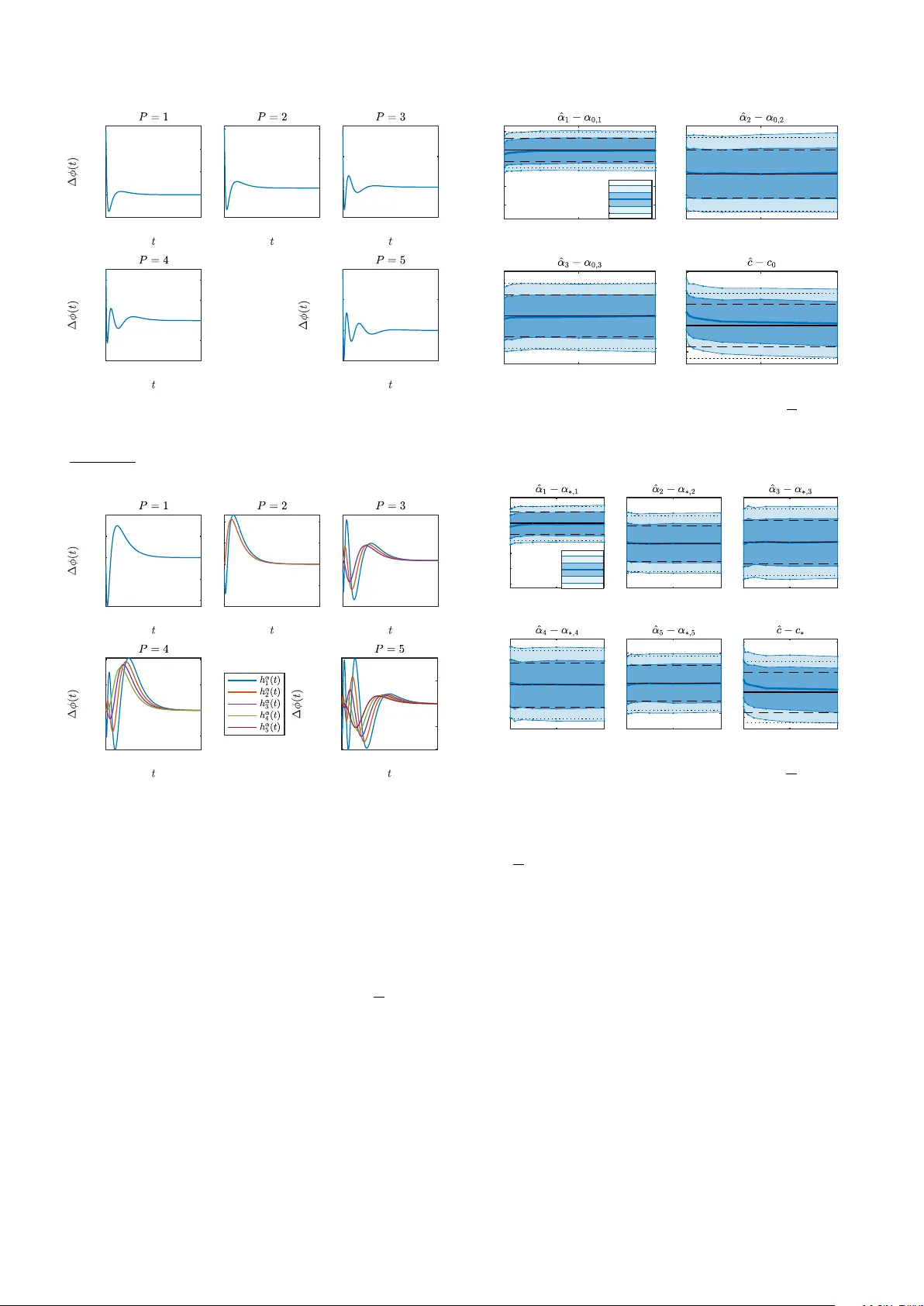
Ha wk es Iden tication with a Prescrib ed Causal Basis: Closed-F orm Estimators and Asymptotics 1 Xinh ui Rong a , Girish N. Nair a a Dep artment of Ele ctric al and Electr onic Engine ering, the University of Melb ourne, A ustr alia Abstract Driv en b y the recent surge in neural-inspired modeling, p oin t processes hav e gained signicant traction in systems and con trol. While the Hawk es pro cess is the standard mo del for characterizing random ev ent sequences with memory , iden tifying its unkno wn k ernels is often hindered by nonlinearity . Approac hes using prescrib ed basis kernels ha v e emerged to enable linear parameterization, y et they t ypically rely on iterative lik eliho o d metho ds and lack rigorous analysis under mo del missp ecication. This pap er justies a closed-form Least Squares identication framework for Hawk es pro cesses with prescrib ed kernels. W e guaran tee estimator existence via the almost-sure p ositive deniteness of the empirical Gram matrix and prov e con vergence to the true parameters under correct specication, or to well-dened pseudo-true parameters under misspecication. F urthermore, w e derive explicit Cen tral Limit Theorems for b oth regimes, providing a complete and interpretable asymptotic theory . W e demonstrate these theoretical ndings through comparative n umerical simulations. K ey wor ds: System Identication, Hawk es Processes, Sto chastic Systems, Asymptotic Analysis. 1 In tro duction The past few decades ha ve witnessed a paradigm shift in the monitoring and understanding of even t-based pro- cesses, driven b y a surge in neural-inspired technologies and the unprecedented av ailabilit y of ev ent data. This shift spans diverse disciplines: from computational neu- roscience [6], where information is enco ded in the pre- cise timing of neural spik es rather than voltage magni- tude; to genomics [10], where transcription ev en ts o c- cur at sp ecic genomic p ositions; to high-frequency - nance [5, 15], where trade timing is critical for infer- ring mark et structure; and so cial media analysis [49], where the causalit y of tw eet and retw eet even ts reveals so cial net work top ology . Consequen tly , these random- ev en t frameworks hav e recently found key applications in con trol and signal pro cessing, including even t-triggered state estimation [43], even t-based vision [17], and mul- titarget radar tracking [18]. P oin t processes [13] pro vide a precise mathematical framew ork for mo delling these even t-based phenomena, dra wing on o ver sixty y ears of theoretical developmen t Email addr esses: xinhui.rong@unimelb.edu.au (Xinhui Rong), gnair@unimelb.edu.au (Girish N. Nair). 1 P art of this manuscript has been presented at the 2026 American Control Conference. across statistics, biometrics, econometrics, etc. Within this framew ork, the Hawk es pro cess [22] stands out as a causal, self-exciting model, serving as the point-process coun terpart to autoregressive mo dels. T raditional maximum likelihoo d estimators (MLEs), im- plemen ted via direct numerical optimization [35] or the exp ectation-maximization (EM) algorithm [19, 28, 45] are a v ailable for the Ha wkes pro cess. Ho wev er, the iden- tication of Hawk es processes remains an active research area, even for the standard linear form. This c hallenge arises b ecause, although the intensit y is linear with re- sp ect to the memory regressor, the regressor itself is de- ned by a con volution of past ev en ts with a deterministic Ha wk es Impulse Resp onse (HIR) that t ypically depends nonlinearly on the parameters, e.g., the exp onen ts. The n um b er of nonlinear parameters grows quadratically as the net w ork dimension, rendering the iterativ e likelihoo d metho ds intractable [12]. Non-parametric Ha wkes modelling [1, 3, 26] circum ven ts the challenges of nonlinear parameter estimation but t ypically relies on binning the pro cess in either the time or frequency domain, which introduces tuning sensitiv- it y and inevitable information loss. An alternativ e ap- proac h av oids binning by mo delling the HIR as a linear com bination of prescrib ed, causal basis functions. In this framew ork, even ts are ltered rather than bin-counted, Preprin t submitted to Automatica 25 F ebruary 2026 preserving the contin uous-time (CT) nature of the data without information loss while rendering the mo del lin- ear in all parameters. Using a prescribed basis (e.g., Hawk es-Laguerre [19, 33]) yields signicant computational adv antages. The EM up dates b ecome closed-form [19, 28]. More imp ortantly , the linearity enables a CT Least-Squares (LS) form ula- tion [2, 21, 31, 39, 42]. This admits p oten tial closed-form estimates, pro vided the empirical Gram matrix is p os- itiv e denite, and oers a m uch more straigh tforward framew ork for incorporating sparsity or other parameter constrain ts. The LS approac h naturally raises three fundamental questions: (1) Under what conditions is the empiri- cal Gram matrix p ositive denite with probabilit y one (w.p.1), thereb y guaran teeing the existence and unique- ness of the closed-form LS estimate? (2) If the true HIR lies within the span of the prescrib ed basis (cor- rect sp ecication), is the LS estimator consistent, and do es it exhibit asymptotic normalit y? (3) In the in- evitable scenario where the true HIR is missp ecied by the prescrib ed basis, do es the estimator conv erge to a w ell-dened pseudo-true parameter, and do es a Central Limit Theorem (CL T) still hold? In the conference version [41] of this paper, we partly answ ered the abov e questions, complementing the exist- ing results. Unlike prior studies that either assume posi- tiv e deniteness or guaran tee it only with high probabil- it y [21], in [41], we established that the empirical Gram matrix is p ositive denite w.p.1 under minimal condi- tions. The second and third questions present signi- can t challenges in Hawk es pro cess iden tication, even within the well-studied MLE framework. Under correct mo del sp ecication, asymptotic consistency and CL T s ha v e b een established for Ha wkes MLEs [11, 27, 32], and consistency has been sho wn for binned processes [26]. In the context of CT LS, while nite-sample risk b ounds exist for penalized estimators [2, 39], we recently deriv ed the rst consistency result for the unp enalized estima- tor in [41], relying on an ergodicity assumption. Re- garding mo del missp ecication, although general quasi- lik eliho o d theory is w ell-established [48], the asymptotic con v ergence of the CT LS estimators remained an op en problem until [41], where we prov ed con vergence in prob- abilit y to pseudo-true parameters under the ergo dicity assumption. Ho wev er, to date, no CL T s hav e b een es- tablished for CT LS estimators under either correct or missp ecied conditions. In this pap er, we substantially strengthen the results of [41] in tw o key asp ects. First, w e replace the general ergo dicit y assumption with explicit causal kernel mo- men t conditions, underpinning the asymptotic analysis and thereby upgrading the conv ergence from ‘in proba- bilit y’ to ‘w.p.1’ . Second, we establish CL T s for CT LS estimators under b oth correct mo del specication and missp ecication. F or the sake of completeness, we also recapitulate the preliminary results from [41], including the existence conditions of the LS estimators. W e fo cus on one-dimensional (not spatial), univ ariate (not net- w ork) linear Hawk es pro cesses. These theoretical ndings substantiate the use of LS Ha wk es iden tication with a prescribed basis, challeng- ing the prev ailing view that LS is merely a secondary alternativ e to MLE. Bey ond these immediate contribu- tions, our results op en the do or to several signican t applications. The explicit nature of the LS estima- tor promises to enable real-time implementation with substan tial computational adv an tages. F urthermore, the deriv ation of explicit pseudo-true parameters and asymptotic co v ariance pav es the wa y for rigorous ro- bustness analysis in future studies. Signicantly , the established CL T s provide the essential theoretical foun- dation for dev eloping Generalized Metho d of Moments (GMM) tests [20], particularly for non-nested mo del comparisons [40, 46] under missp ecication. The remainder of this paper is organized as follows. Sec- tion 2 and Section 3 review the necessary preliminar- ies on the general p oint processes and key lemmas for Ha wk es processes. Section 4 form ulates the CT LS prob- lem, derives the closed-form estimators, and establishes their nite-time existence. Section 5 analyzes the asymp- totic behavior of the estimators, proving conv ergence to the true parameters under correct sp ecication and to w ell-dened pseudo-true parameters under missp ecica- tion. Section 6 deriv es the CL T s for b oth sp ecication regimes, providing explicit and interpretable expressions for the asymptotic cov ariances. Section 7 presents a nu- merical study that computes pseudo-true v alues, con- ducts an asymptotic robustness analysis of the Hawk es- Laguerre mo del, and v alidates the asymptotic prop erties of the LS estimator. Section VII I con tains conclusions and future work. 2 Preliminaries In this section, we introduce the mathematical c harac- terization of p oint pro cesses and review the fundamental notations required for our analysis. A p oint process is a pro cess of random even t times. De- note the strictly increasing sequence of even t times (e.g., the timings of neural spikes) by { t r } r ∈ Z . The c ounting pr o c ess N t represen ts a p oint pro cess and is dened by N t ≜ N (( −∞ , t ]) = P r ∈ Z 1 t ≥ t r , where N ( A ) measures the num b er of even ts in a Borel set A ⊂ R and 1 t ∈ A = { 1 , t ∈ A 0 , t / ∈ A is the indicator function. By denition, N t is a right-con tinuous non-decreasing step function that jumps by one at each even t time. 2 T o characterize the dynamics, it is conv enient to work with the dierential increment of N t . Heuristically , the coun ting incremen t dN t = P t r ≤ t δ ( t − t r ) dt can b e in- terpreted as a train of Dirac impulses δ lo calized at the ev en t times. This in terpretation allows us to dene l- tering operations via Riemann-Stieltjes conv olution. F or a causal kernel function g : [0 , ∞ ) 7→ R and an obser- v ation window A ⊂ R , the Riemann-Stieltjes con v olu- tion of the k ernel with the coun ting process is dened as R A g ( t − u ) dN u = P t r ∈ A g ( t − t r ) . Throughout, we adopt the standard or derliness assump- tion: lim τ → 0 1 τ Pr[ N ([ t, t + τ )) > 1] = 0 , ∀ t ∈ R , which suggests that simultaneous ev ents are not allow ed in an innitesimal in terv al. Let H t − = σ { N s , s < t } b e the history/ltration of the counting pro cess. The (c ondi- tional) intensity function λ is dened as λ ( t ) = lim τ → 0 1 τ E[ N ([ t, t + τ )) |H t − ] , (2.1) the instan taneous probability rate of a future ev ent, con- ditioned strictly on the past history . The in tensity func- tion λ uniquely characterizes a p oint pro cess. W e need to in tro duce some basic notations. Let g , f : R → R be deterministic functions. W e denote ¯ g ( s ) = R ∞ −∞ e − st g ( t ) dt the Laplace transform (L T) of g and ¯ g ( ȷω ) is, therefore, the F ourier transform (FT) of g . W e denote g ⋆ f ( t ) = R ∞ −∞ g ( t − u ) f ( u ) du the con volu- tion of f and g . W e denote g ⋆ dN t = R t − −∞ g ( t − u ) dN u the Riemann-Stieltjes con volution. W e will also write | g | ⋆ dN t = R t − −∞ | g ( t − u ) | dN u . W e denote f ⋆n ( t ) = f ⋆ f ⋆ · · · ⋆ f ( t ) the n -fold con volution of f . These denitions also extend when g : R 7→ R k is a v ector of functions. When we put the absolute sign on a vector g ( t ) = [ g 1 ( t ) , · · · , g P ( t )] ⊤ , w e mean | g ( t ) | = [ | g 1 ( t ) | , · · · , | g P ( t ) | ] ⊤ . The L p norm is de- ned as k f k L p = R R | f ( t ) | p dt 1 /p , 1 ≤ p < ∞ and k f k L ∞ = sup t ∈ R | f ( t ) | . W e denote L p [0 , ∞ ) , 1 ≤ p ≤ ∞ the L p space of functions f : R 7→ R suc h that f ( t ) = 0 , t < 0 and their L p norm k f k L p exists. Let 1 P denote a P -dimensional vector of 1 ’s. The nota- tion o p ( 1 P ) represents a sequence of P -dimensional random vectors that con v erges to zero in probabilit y . The notation a.e. stands for almost ev erywhere, the notation p − → stands for con v ergence in probability , and X T = ⇒ N (0 , Σ) means that X T con v erges in distri- bution to a zero-mean Gaussian random v ariable with co v ariance matrix Σ . 3 Ha wkes Modelling The Hawk es pro cess is the most widely used mo del for history-dep endent even t sequences, serving as the p oint- pro cess coun terpart to the autoregressiv e mo del in time series. This section reviews the Ha wkes intensit y and the fundamen tal prop erties that establish the basis for our analysis and motiv ate the assumptions adopted in this w ork. 3.1 The Hawkes Intensity A Hawk es pro cess is a self-exciting point process uniquely characterized by the intensit y function λ 0 ( t ) = c 0 + χ 0 ( t ) (3.1a) χ 0 ( t ) = ϕ 0 ⋆ dN t = Z t − −∞ ϕ 0 ( t − u ) dN u (3.1b) with ϕ 0 ( t ) ≥ 0 , ϕ 0 ∈ L 1 [0 , ∞ ) ∩ L ∞ [0 , ∞ ) , (3.1c) and Γ = k ϕ 0 k L 1 < 1 , c 0 > 0 . (3.1d) c 0 is the deterministic b ackgr ound r ate , χ 0 is a sto chastic memory pr o c ess , which is the self-exciting comp onent of the in tensit y , ϕ 0 is the deterministic Hawkes impulse r esp onse (HIR), c haracterizing the additive increase in the intensit y induced by eac h past even t, and Γ is the br anching r atio . The conditions on the HIR ϕ 0 are to ensure the almost- sure p ositivity and b oundedness of the intensit y λ 0 as w ell as the stationarit y , which underpins the key prop- erties, to b e in tro duced next. The in terp olation inequal- it y [16] ensures k ϕ 0 k L p ≤ k ϕ 0 k 1 /p L 1 k ϕ 0 k 1 − 1 /p L ∞ < ∞ , for an y 1 < p < ∞ . By denition, the Hawk es intensit y λ 0 is left-contin uous with right limits, so that it is an H t − - predictable sto chastic pro cess [8]. Under a Hawk es in tensity (3.1), the deterministic Hawkes r esolvent is dened as ψ ( t ) = ∞ X n =1 ϕ ⋆n 0 ( t ) , t ≥ 0 . (3.2) The existence of the Ha wkes resolven t ψ is guaranteed by the condition Γ ∈ (0 , 1) and it is straigh tforward to sho w that k ψ k L p < ∞ for all 1 ≤ p ≤ ∞ recursively using the Y oung’s conv olutional inequalit y and that k ψ k L 1 = P ∞ n =1 k ϕ 0 k L 1 = Γ 1 − Γ b y recursively using the identit y k ϕ ⋆ 2 0 k L 1 = k ϕ 0 k 2 L 1 . The Hawk es resolven t has L T ¯ ψ ( s ) = ¯ ϕ 0 ( s ) 1 − ¯ ϕ 0 ( s ) , (3.3) and is closely related to the higher-order statistics of the coun ting pro cess and our asymptotic analysis. 3.2 K ey L emmas Here, we summarize key prop erties of Ha wk es processes, including stationarity and ergo dicity of the counting pro- cess, moments and cumulan ts, and martingale dynamics. 3 These results are either standard or follow immediately from known prop erties, with short deriv ations included for completeness. Lemma 1 Stationarit y . [9] Ther e exists a unique strictly stationary distribution for the c ounting pr o c ess N t , char acterize d by (3.1). Lemma 2 Ergodicity . A stationary Hawkes c ounting pr o c ess with (3.1) is er go dic 2 . Pr o of. A stationary cluster process is ergodic if its clus- ter center is [14, Proposition 12.3.IX]. A Hawk es process with (3.1) is a P oisson cluster pro cess [23] whose clus- ter cen ter follows a time-inv arian t Poisson pro cess. Since the time-in v ariant Poisson pro cess is ergo dic [14, Exer- cise 12.3.1], the resulting counting pro cess is ergo dic. □ The following Lemmas 3-5 summarize prop erties of the cum ulan ts of the counting increments. W e require the explicit form ulae for the rst and second cum ulants and the existence of all higher-order integrated moments. Lemma 3 First order statistics. [22] F or a station- ary Hawkes pr o c ess with (3.1), the exp e cte d c ounting in- cr ement is given by 3 E[ dN t ] /dt = E[ λ 0 ( t )] = E[ λ 0 (0)] = Λ , wher e Λ = c 0 1 − Γ is the exp e cte d r ate. Lemma 4 Second order statistics. F or a stationary Hawkes pr o c ess with (3.1), (a) the c ovarianc e density of N is given by C ( u − v ) = E[ dN u dN v ] − E[ dN u ] E[ dN v ] dudv = C ( v − u ) . (b) F urther, the Bartlett’s sp e ctrum, which is the FT of C and given by 4 ¯ C ( ω ) = Λ | 1 − ¯ ϕ ( ȷω ) | 2 , (3.4) exists, is r e al, and is strictly p ositive at any ω ∈ R . (c) The c ovarianc e density C ( τ ) c ontains a singular spike 2 An ergo dic counting pro cess N has a trivial inv ariant σ - algebra under the measure-preserving shift op erations. See [14, Chapter 12] for full details. 3 Throughout the paper, the expectation E , the probability Pr , the v ariance V ar , and the cov ariance Cov are taken with resp ect to the unique stationary probabilit y measure of the coun ting pro cess N dened b y the in tensity (3.1). 4 W e write ¯ C ( ω ) instead of ¯ C ( ȷω ) to denote that the sp ec- trum is real. at the origin and a b ounde d r e gular p art as fol lows. C ( τ ) = Λ δ ( τ ) + C reg ( τ ) (3.5) C reg ( τ ) = Λ( ψ ( τ ) + ˇ ψ ( τ ) + ψ ⋆ ˇ ψ ( τ )) , (3.6) wher e δ ( τ ) is the Dir ac delta function c enter e d at 0 , ˇ ψ ( τ ) = ψ ( − τ ) , C reg is symmetric, non-ne gative, and b ounde d, and k C k L 1 = Λ (1 − Γ) 2 < ∞ . Pr o of. Results (a,b) are in [22] and [5]. The existence and strict positivity of ¯ C ( ω ) follows from | ¯ ϕ ( ȷω ) | ≤ Γ < 1 . Result (c) can be found in [3] or b e directly deriv ed from the FT (3.4). The symmetry of C reg is obvious from its denition. The b oundedness of C reg follo ws by noticing k ψ k L ∞ = k ˇ ψ k L ∞ and using Y oung’s inequalit y to get k ψ ⋆ ˇ ψ k L ∞ ≤ k ψ k L ∞ k ψ k L 1 < ∞ . k C k L 1 = Λ( k δ k L 1 + 2 k ψ k L 1 + k ψ k 2 L 1 ) = Λ(1 + Γ 1 − Γ ) 2 = Λ (1 − Γ) 2 . □ Lemma 5 Higher-order statistics. [25] F or a sta- tionary Hawkes pr o c ess with (3.1) , the n -th inte gr ate d moment is given by Z [ τ 1 , ··· ,τ n − 1 ] ⊤ ∈ R n − 1 E[ dN t dN t + τ 1 · · · dN t + τ n − 1 ] = K n dt, wher e the c onstant K n ∈ (0 , ∞ ) is b ounde d for al l n ∈ N and admits a r e cursive expr ession r e gar ding Λ and k C k L 1 given in [25, Se ction IV]. The predictabilit y of the Hawk es intensit y λ 0 and the nite expected rate under Γ < 1 ensures the existence of the unique Doob-Meyer decomp osition to construct a martingale. W e dene the trunc ate d c ounting pr o c ess ˜ N t = N ((0 , t ]) , and M t = ˜ N t − R t 0 λ 0 ( u ) du, dM t = dN t − λ 0 ( t ) dt, t > 0 . Lemma 6 Martingales dynamics. [8, Chapter II] F or a stationary Hawkes pr o c ess with (3.1), (a) M t is an H t − -martingale, i.e. for any t ≥ 0 , E[ ˜ N t − R t 0 λ 0 ( u ) du |H 0 − ] = 0 . (b) If h ( t ) is an H t − -pr e dictable pr o c ess such that E[ R t 0 | h ( u ) | λ 0 ( u ) du ] < ∞ , t ≥ 0 , then R t 0 h ( u ) dM u is an H t − -martingale, i.e. for any t ≥ 0 , E[ R t 0 h ( t ) d ˜ N t − R t 0 h ( t ) λ 0 ( t ) dt |H 0 − ] = 0 . 4 Least-Squares Iden tication for Ha wkes In this section, we imp ose the fundamental mo delling assumptions, formulate the LS iden tication problem, and detail the closed-form estimators originally derived 4 in our conference pap er [41]. These results are restated here to ensure the exp osition is self-contained and to establish the necessary framework for the asymptotic analysis in subsequent sections. 4.1 T runc ate d Observation While the theoretical pro cess extends to the innite past, practical applications are limited to nite observ ation in terv als. W e therefore work with the truncated count- ing pro cess ˜ N t , observed in a deterministic time p erio d (0 , T ] . F or the sake of simplicity , w e assume that the coun ting pro cess is stationary . A1 Stationarit y and Observ ation. The observe d c ounting pr o c ess ˜ N t = N ((0 , t ]) is a trunc ation of the stationary c ounting pr o c ess N t with the unknown true intensity (3.1) , over the time interval t ∈ (0 , T ] . Under A1, the full counting pro cess N t is stationary and ergo dic, satisfying all prop erties in Lemmas 1-5. The truncated counting pro cess ˜ N t satises Lemma 6 and its incremen t d ˜ N t preserv es stationarity . 4.2 The Candidate Intensity and its T runc ation The iden tication ob jective is to estimate b oth the back- ground rate c 0 and the HIR ϕ 0 . How ever, the nonlinear parameterization of ϕ 0 t ypically poses signicant esti- mation challenges. T o circumv ent this, it is a common practice to approximate ϕ 0 ( t ) = P j α j q j ( t ) using a lin- ear combination of prescrib ed causal basis functions q j , e.g. the Ha wkes-Laguerre mo del [19]. This leads to the denition of the following linear candidate intensit y λ 1 ( t ; θ ) = c + α ⊤ χ ( t ) , t ∈ R (4.1a) χ ( t ) = q ⋆ dN t = Z t − −∞ q ( t − u ) dN u ∈ R P , (4.1b) where c is the candidate background rate, α = [ α 1 , α 2 , · · · , α P ] ⊤ is the weigh ting parameter with mo del order P , θ = [ α ⊤ , c ] ⊤ ∈ R P +1 is the parame- ter vector, and χ ( t ) = [ χ 1 ( t ) , · · · , χ P ( t )] ⊤ is a vector of the candidate memory regressor, where the deter- ministic q ( t ) = [ q 1 ( t ) , · · · , q P ( t )] ⊤ is the vector of prescrib ed/user-dened unit mass c ausal kernels (UM- CKs) with each UMCK q j ∈ L 1 [0 , ∞ ) ∩ L ∞ [0 , ∞ ) , and q j ( t ) ≥ 0 and k q j k L 1 = 1 . W e also dene ϕ 1 ( t ) = α ⊤ q ( t ) as the candidate HIR. Since, again, the ev ents b efore time 0 are not observ ed, to identify the candidate intensit y , we need to work with its truncated version ˜ λ 1 ( t ; θ ) = c + α ⊤ ˜ χ ( t ) , t ∈ [0 , T ] (4.2a) ˜ χ ( t ) = q ⋆ d ˜ N t ≜ Z t − 0 q ( t − u ) dN u ∈ R P , (4.2b) where ˜ χ ( t ) ∈ R P is the truncated memory regressor and w e dene the truncated Riemann-Stieltjes conv olution as g ⋆ d ˜ N t = R t − 0 g ( t − u ) d ˜ N u of a causal function g : [0 , ∞ ) 7→ R k with the truncated coun ting pro cess ˜ N on [0 , t ) . T o av oid confusion, we note that since N and ˜ N share the same increments on (0 , T ] , g ⋆ d ˜ N t = R t 0 g ( t − u ) dN u = R t 0 g ( t − u ) d ˜ N u . Subsequently , we will also write | g | ⋆ d ˜ N t = R t − 0 | g ( t − u ) | dN u . W e note that the truncated pro cesses lose stationarity . Thanks to the prescribed UMCKs, giv en an observ ation ˜ N , the truncated memory regressor ˜ χ is fully observed in (0 , T ] , leading to a linear parameterization of ˜ λ 1 in regard to the parameter θ . F or future use, we dene ∆ χ ( t ) = χ ( t ) − ˜ χ ( t ) (4.3) with ∆ χ j ( t ) = χ j ( t ) − ˜ χ j ( t ) , j = 1 , · · · , P = Z 0 − −∞ q j ( t − u ) dN u > 0 . (4.4) W e also dene the truncated true (latent) memory pro- cess as ˜ χ 0 ( t ) = R t − 0 ϕ 0 ( t − u ) dN u and ∆ χ 0 ( t ) = χ 0 ( t ) − ˜ χ 0 ( t ) = R 0 − −∞ ϕ 0 ( t − u ) dN u > 0 . The prescribed UMCKs need to satisfy the following iden tiabilit y condition which also guaran tees a unique LS estimator to b e dev elop ed next. A2 Iden tiable UMCKs. The c andidate UMCK s satisfy the fol lowing c onditions. (a) Density-like: q j ∈ L 1 [0 , ∞ ) ∩ L ∞ [0 , ∞ ) with q j ( t ) ≥ 0 and k q j k L 1 = 1 for al l j . (b) Finite-horizon ane indep endenc e: Ther e exists a nite t 0 > 0 , such that ther e is no p air of x 6 = 0 ∈ R P and d ∈ R , such that x ⊤ q ( t ) = d , a.e. on t ∈ [0 , t 0 ] . (*) W e dene the minimal ane-indep endenc e horizon T 0 to b e the inmum of such t 0 for which A2(b) is satise d. W e note that A2(a) is just a conv enient rescaling of the HIR basis and that the interpolation inequality [16] ensures k q j k L p < ∞ for any 1 ≤ q ≤ ∞ . A2(b) strength- ens ordinary linear independence in t wo respects: (i) it enforces indep endence on the nite horizon [0 , t 0 ] , and (ii) it requires ane indep endence. Equiv alen tly , { 1 , q 1 , · · · , q P } is linearly indep endent a.e. on [0 , t 0 ] . These strengthenings ensure the existence and unique- ness of the LS estimator developed next. The assump- tion is mild and holds with T 0 = 0 for most prescrib ed UMCKs (e.g., exp onential [22] and Erlang bases [19]). If the candidate kernels are linearly indep endent but an y one of them is constant on an initial interv al, then T 0 equals the rst time at which every kernel b ecomes time-v arying. Since q j ’s are prescrib ed, T 0 is alwa ys kno wn and can alwa ys b e designed to b e 0 . 5 4.3 The L e ast-Squar es F ormulation Supp ose we observe a truncated counting pro cess with strictly increasing even t times t 1 , t 2 , . . . ov er a de- terministic interv al (0 , T ] . W e dene the truncated extended regressor as ˜ ξ ( t ) = [ ˜ χ ( t ) ⊤ , 1] ⊤ ∈ R P +1 , where the app ended constan t accounts for the mem- oryless bac kground rate. While the contin uous-time least squares (LS) contrast, J T ( θ ) given b elow, is well- established [2, 21], we decompose its key terms to yield a more interpretable LS estimator and streamline its asymptotic analysis. J T ( θ ) = 1 T Z T 0 ˜ λ 1 ( t ; θ ) 2 dt − 2 T Z T 0 ˜ λ 1 ( t ; θ ) dN t = θ ⊤ G T θ − 2 θ ⊤ g T , (4.5) where G T = 1 T R T 0 ˜ ξ ( t ) ˜ ξ ( t ) ⊤ dt = h R T + ˆ χ T ˆ χ ⊤ T ˆ χ T ˆ χ ⊤ T 1 i is the empirical Gram matrix and g T = [( s T + ˆ Λ T ˆ χ T ) ⊤ , ˆ Λ T ] ⊤ ∈ R P +1 , where w e dene the scalar ˆ Λ T = ˜ N T /T as the empirical rate, the vector ˆ χ T = 1 T R T 0 ˜ χ ( t ) dt ∈ R P as the memory regressor mean, and R T = 1 T Z T 0 ˜ χ ( t ) ˜ χ ( t ) ⊤ dt − ˆ χ T ˆ χ ⊤ T ∈ R P × P (4.6) s T = 1 T Z T 0 ˜ χ ( t ) dN t − ˆ Λ T ˆ χ T ∈ R P = ˆ V T T − M T T ˆ χ T + R (1 , 0) T , (4.7) where the equiv alent expression (4.7) of s T re- sults from the martingale property in Lemma 6(a), ˆ V T = R T 0 ˜ χ ( t ) dM t and the cross-cov ariance term is R (1 , 0) T = 1 T Z T 0 ˜ χ ( t ) χ 0 ( t ) dt − ˆ χ T 1 T Z T 0 χ 0 ( t ) dt, (4.8) Equations (4.6) and (4.7) admit a statistical in terpreta- tion. R T represen ts the empirical cov ariance of the can- didate memory regressors. Provided that the sto chastic in tegral ˆ V T in (4.7) satises the conditions of Lemma 6 to be a martingale, s T functions as a cross-cov ariance estimator b etw een the truncated candidate memory re- gressor ˜ χ ( t ) and the true memory pro cess χ 0 ( t ) . 4.4 Main R esult I: The L e ast-Squar es Estimator All ˆ Λ , ˆ χ T , g T , s T , R T , G T are fully observ ed, thanks to the prescribed UMCKs. If the empirical Gram matrix G T is p ositive denite, the LS estimator can b e easily ob- tained using the classical matrix calculus [30]. Ho wev er, t w o issues require attention. First, the empirical Gram matrix must b e p ositive denite for nite T . Second, the closed-form LS solution requires a compact form for b oth in terpretation and asymptotic analysis. W e settle b oth issues in the theorem b elo w and presen t the closed-form LS estimators, which rst app eared in our conference v ersion [41]. Theorem 7 Ha wk es LS Estimators. [41] Denote t 1 the time of the rst event, let T b e the deterministic obser- vation time, and T 0 b e the deterministic minimal ane- indep endenc e horizon as dene d in A2(*). Under A1 and A2, if t 1 < T − T 0 , b oth R T and G T ar e p ositive denite, almost sur ely. Then, the LS estimator is given by ˆ θ = " ˆ α ˆ c # = arg min θ ∈ R P +1 J T ( θ ) = G − 1 T g T . F urther, using Schur c omplement [30], we have G − 1 T = R − 1 T − R − 1 T ˆ χ T − ˆ χ ⊤ T R − 1 T ˆ χ ⊤ T R − 1 T ˆ χ T +1 . Ther efor e, ˆ α = R − 1 T s T (4.9) ˆ c = ˆ Λ T − ˆ χ ⊤ T ˆ α. (4.10) Pr o of. Supp ose G T > 0 . By matrix p erturbation [30], it is straigh tforward to show that ˆ θ = G − 1 T g T uniquely minimizes J T ( θ ) . Since the b ottom-right elemen t of G T is 1 > 0 , due to Sch ur complemen t, G T > 0 i R T > 0 . Then the inv ersion G − 1 T using Sc h ur complemen t directly results in the equiv alent form of ˆ θ giv en in (4.9) and (4.10). In App endix A, we complete the pro of b y sho wing R T > 0 almost surely for all T > t 1 + T 0 . □ The interpretation of the theorem is as follows. The LS estimators are guaranteed to exist, subject to a minimal data suciency condition. Dene E T = { t 1 < T − T 0 } . On E T , b oth R T and G T are p ositive denite almost surely , and the closed-form estimators (4.9)–(4.10) are w ell-dened. On the complemen t of E T , the memory regressors are anely dep endent on [0 , T ] , the model is uniden tiable on that horizon, and R T is not p ositiv e denite. Consequently , Pr[ R T > 0] = Pr[ E T ] . Under A1, Pr[ E T ] → 1 as T → ∞ . F or nite T , verifying E T is then a necessary iden tiability chec k. In the typical case of T 0 = 0 (see discussions after A2), the condition b ecomes “at least one even t m ust be observ ed”, whic h is trivial in practice. Regarding the Gram matrix, prior work either assumes p ositive deniteness [31] or shows it only with high prob- abilit y [21] (without the simple, observ able chec k as we do). The equiv alent estimates (4.9) and (4.10) hav e the follo wing prop erties. Remark 1 Mass Conserv ation. R e or ganize (4.10) to nd ˜ N T = ˆ cT + R T 0 ˜ χ ( t ) ⊤ dt ˆ α = R T 0 ˜ λ 1 ( t ; ˆ θ ) dt . Thus, 6 the tte d c andidate intensity inte gr ates to the observe d c ount, despite p ossible missp e cic ation. The same pr op- erty holds for EM estimators (Se e [19, R esult VI]). Remark 2 Relation to the Cen tered LS. The c en- ter e d LS (CLS) 5 sets c = ˆ Λ T − ˆ χ ⊤ T α in (4.5) so that the c orr esp onding LS c ontr ast J ′ T ( α ) only r elies on α . The CLS sep ar ates α ’s and c and, ther efor e, oers a mor e suitable formulation for p ar ameter c onstr aints [36, 42]. It is str aightforwar d to se e ˆ α is the minimizer of the CLS c ontr ast J ′ T ( α ) and ˆ c is exactly the CLS estimator by r e c overing the c entering. This shows that the (unc on- str aine d) LS and CLS ar e e quivalent. 5 Asymptotic Con vergence This section establishes the almost-sure asymptotic con- v ergence of the LS estimators. W e prov e that the es- timators are strongly consistent when the true HIR is spanned by the candidate UMCKs, and conv erge to well- dened pseudo-true parameters otherwise. These results strengthen our preliminary w ork [41] by strengthening con v ergence in probability to con vergence w.p.1 and re- placing the explicit ergo dicity assumption directly on memory regressors with m uch more general conditions on the causal kernels. W e b egin by formally dening a correct sp ecication. The subsequent subsections then establish the funda- men tal assumptions and key lemmas that underpin the asymptotic analysis. The main results are presented in Section 5.3. Denition 8 Correct sp ecication. The c andidate intensity λ 1 ( t ; θ ) c orr e ctly sp e cies the true Hawkes pr o- c ess if A1 and A2 ar e satise d, and ther e exists a unique α 0 ∈ R P such that ϕ 0 ( t ) = α ⊤ 0 q ( t ) , a.e. on t ∈ [0 , ∞ ) . In this c ase, we dene θ 0 = [ α ⊤ 0 , c 0 ] ⊤ as the true p ar am- eters. 5.1 A n Er go dic L emma W e present an ergo dic lemma that establishes the fun- damen tal ergo dic prop erties required for our asymptotic analysis. Lemma 9 Ergodic Lemma. L et N b e a stationary c ounting pr o c ess satisfying A1 and g j ∈ L 1 [0 , ∞ ) ∩ L ∞ [0 , ∞ ) , j ∈ N b e deterministic functions. Dene the sto chastic pr o c esses f j ( t ) = g j ⋆ dN t , j ∈ N . (a) F or al l n ∈ N , Q j ∈P n f j ( t ) , P n = { 1 , 2 , · · · , n } ar e stationary with E[ Q j ∈P n f j ( t )] = E[ Q j ∈P n f j (0)] < ∞ . 5 See [42] for a deriv ation for the con tinuous-time CLS and [36] for a discrete-time version. (b) Sp e cial ly, E[ λ 0 ( t ) n ] = E[ λ 0 (0) n ] < ∞ , ∀ n ∈ N E[ f j (0)] =Λ R ∞ 0 g j ( u ) du Co v[ f 1 (0) , f 2 (0)] = E[ f 1 (0) f 2 (0)] − E[ f 1 (0)] E[ f 2 (0)] = R ∞ 0 R ∞ 0 g 1 ( v ) g 2 ( u ) C ( u − v ) dv du. (c) F urther, for al l n ∈ N , as T → ∞ , 1 T Z T 0 Q j ∈P n f j ( t ) dt → E[ Q j ∈P n f j (0)] , w.p.1 . 5.2 K ernel Conditions and the V anishing Bias T erms Lemma 9 alone is insucien t to establish the required con v ergence, as our analysis in volv es non-stationary truncated pro cesses. W e must further demonstrate that the bias terms, arising from unobserv ed pre-sample ev en ts and the martingale dierences, v anish asymptot- ically w.p.1. T o achiev e this, we introduce the following regularit y conditions. A3 Kernel regularity conditions. (a) F or the true HIR, R ∞ 0 tϕ 0 ( t ) dt < ∞ . (b) F or the UMCK s, R ∞ 0 tq j ( t ) dt < ∞ , j ∈ { 1 , · · · , P } . A3 is imp osed to ensure that the inuence of the unob- serv ed history prior to time 0 v anishes asymptotically in the truncated statistics [9]. This condition is mild and widely satised; it holds for all kernels with exp onen- tial tails (e.g., the standard Hawk es-exp onen tial [22] and Ha wk es-Laguerre [19] mo dels) as well as for heavy-tailed k ernels with a nite mean. Lemma 10 V anishing drift terms. L et N b e a sta- tionary Hawkes pr o c ess with (3.1) . L et g j ∈ L 1 [0 , ∞ ) ∩ L ∞ [0 , ∞ ) , j ∈ N and h j ∈ L 1 [0 , ∞ ) , j ∈ N b e determinis- tic functions. Dene ∆ f 1 ( t ) = R 0 − −∞ g 1 ( t − τ ) dN τ to b e the pr e-zer o memory and f A j j ( t ) = R A j g j ( t − τ ) dN τ , A j ⊆ R . If R ∞ 0 t | g 1 ( t ) | dt < ∞ , then for any ϵ > 0 , as T → ∞ , the fol lowing pr o c esses c onver ge to 0 w.p.1: 1 T ϵ Z T 0 h 1 ⋆ ∆ f 1 ( t ) n Y j =2 h j ⋆ f A j j ( t ) dt, 1 T ϵ Z T 0 h 1 ⋆ ∆ f 1 ( t ) dN t , 1 T ϵ Z T 0 h 1 ⋆ ∆ f 1 ( t ) dM t . Lemma 10 will simplify the analysis of the truncated pro- cesses. W e decomp ose the truncated process (e.g. ˜ χ ( t ) = R t − 0 q ( t − u ) dN u ) in to the dierence b etw een the station- ary pro cess (e.g. χ ( t ) = R t − −∞ q ( t − u ) dN u ) and the pre- zero memory pro cess (e.g. ∆ χ ( t ) = R 0 − −∞ q ( t − u ) dN u ). 7 By setting h j in Lemma 10 to the Dirac delta function δ (note that k δ k L 1 = 1 ), the av eraging terms in v olving the pre-zero memory process v anish w.p.1. This isolates the stationary comp onents, allowing us to directly ap- ply Lemma 9. The following Lemma 11 will establish the con v ergence of s T as a cross-cov ariance estimator. Lemma 11 Martingales in integral forms. L et N b e a stationary Hawkes pr o c ess with (3.1) . L et g j ∈ L 1 [0 , ∞ ) ∩ L ∞ [0 , ∞ ) b e deterministic functions and f j ( t ) = g j ⋆ dN t , ˜ f j = g j ⋆ d ˜ N t b e sto chastic pr o c esses. Dene M f j,t = R t − 0 f j ( u ) dM u and ˜ M f j,t = R t − 0 ˜ f j ( u ) dM u . (a) Both M f j,t , ˜ M f j,t ar e H t − -martingales. (b) 1 T M f j,T → 0 , 1 T ˜ M f j,T → 0 w.p.1, as T → ∞ . 5.3 Main R esult II: A symptotic Conver genc e Here, w e presen t the key conv ergence results that es- tablish the conv ergence of the LS estimators. W e list the con vergence of ˆ Λ T , ˆ χ T , R T , R (1 , 0) T , s T as lemmas and conclude the conv ergence of the LS estimator b y the con- tin uous mapping theorem in Theorem 15 b elo w. Lemma 12 Under A1-A3, as T → ∞ , ˆ χ T → µ ≜ E[ χ (0)] = Λ 1 P , w.p.1. , (5.1) wher e 1 k is a k -dimensional ve ctor of 1 ’s. Lemma 13 Under A1-A3, (a) as T → ∞ , the c ovarianc e estimators R T → R ∗ , w.p.1. R (1 , 0) T → R (1 , 0) ∗ , w.p.1. , wher e R ∗ , R (1 , 0) ∗ exist with R ∗ > 0 and ar e given by R ∗ ≜ V ar[ χ (0)] = E χ (0) χ (0) ⊤ − µµ ⊤ = Z ∞ 0 Z ∞ 0 q ( u ) C ( u − v ) q ( v ) ⊤ dudv (5.2) R (1 , 0) ∗ ≜ Cov[ χ (0) , ϕ 0 (0)] = E [ χ (0) ϕ 0 (0)] − Γ µ = Z ∞ 0 Z ∞ 0 q ( u ) C ( u − v ) ϕ 0 ( v ) dudv . (5.3) (b) By Parseval’s the or em [34], R ∗ = 1 2 π Z ∞ −∞ ¯ q ( ȷω ) ¯ C ( ω ) ¯ q ( − ȷω ) ⊤ dω (5.4) R (1 , 0) ∗ = 1 2 π Z ∞ −∞ ¯ q ( ȷω ) ¯ C ( ω ) ¯ ϕ 0 ( − ȷω ) dω . (5.5) Lemma 14 Consider s T in (4.7) . Under A1-A3, (a) ˆ V T = R T 0 ˜ χ ( t ) dM t is an H T − -martingale, (b) as T → ∞ , ˆ V T T → 0 , M T T → 0 , w.p.1, and (c) as T → ∞ , s T → R (1 , 0) ∗ , w.p.1. The ab ov e conv ergences and the p ositive deniteness of R ∗ lead to the conv ergence of the LS estimators. Theorem 15 Strong consistency of the LS estima- tors. Under A1-A3, the LS weighting estimator ˆ α and the LS b ackgr ound r ate estimator ˆ c b oth c onver ge w.p.1 to their pseudo-true values ˆ θ → θ ∗ = [ α ⊤ ∗ , c ∗ ] ⊤ , given by α ∗ = R − 1 ∗ R (1 , 0) ∗ (5.6) c ∗ = Λ − µ ⊤ α ∗ = Λ(1 − Γ ∗ ) , (5.7) wher e we dene Γ ∗ = 1 ⊤ P α ∗ as the pseudo-true br anching r atio. In the c ase of c orr e ct sp e cic ation, the LS estima- tors ar e c onsistent: α ∗ = α 0 and c ∗ = c 0 . Pr o of. The rst set of conv ergences follows from Lem- mas 12-14 and the contin uous mapping theorem. The frequency domain expression follows by noticing, e.g., R ∞ 0 R ∞ 0 q ( u ) C ( u − v ) q ( v ) ⊤ dv du = R ∞ 0 q ⋆ C ( u ) q ( u ) ⊤ du and then applying Parsev al’s theorem [34]. Consis- tency follows by noticing that, under correct sp eci- cation, ϕ 0 ( t ) = q ( t ) ⊤ α 0 , so we hav e R (1 , 0) ∗ = R ∗ α 0 ⇒ R − 1 ∗ R (1 , 0) ∗ = α 0 and c ∗ = Λ(1 − 1 ⊤ P α 0 ) = Λ(1 − Γ) = c 0 , b y Lemma 3. □ Theorem 15 provides a fundamental justication for Ha wk es mo deling with prescrib ed basis k ernels in tw o k ey asp ects. First, under correct sp ecication, where the true HIR lies within the span of the known basis functions, the LS estimators are strongly consistent with the true parameters. Second, since the true basis is rarely kno wn in practice, we establish that under missp ecication, the estimators still conv erge w.p.1 to w ell-dened pseudo-true parameters. This con vergence is guaranteed b y the existence of the limiting R ∗ and R (1 , 0) ∗ , and the p ositive deniteness of R ∗ . Theorem 15 strengthens previous MLE results in the literature in the following asp ects. Existing literature, e.g. [11] and [27], imp oses explicit high-order moment assumptions on the intensit y , suc h as E[ λ 0 (0) 3+ ϵ ] < ∞ for some ϵ > 0 . In con trast, we derive these momen t prop erties directly from the primitive conditions on the k ernels. While analyses of MLEs often rely on w eak la ws of large num b ers [11, 27, 32] due to the tec hnical di- cult y of handling the logarithm of the intensit y , the LS framew ork yields conv ergence w.p.1. Another ma jor ad- v an tage of the closed-form LS estimators is that consis- tency follows from the point wise ergo dic con v ergence. 8 This bypasses the need for uniform la ws of large num b ers o v er the parameter space, which are strictly required for M-estimators like the MLE. 6 Cen tral Limit Theorems In this section, w e deriv e the CL T s for the LS estima- tors under b oth correct sp ecication and missp ecica- tion. The closed-form LS estimators allo w us to develop the asymptotic Gaussian co v ariances with explicit, in- terpretable structures. The deriv ation under correct sp ecication, as we shall see b elo w, follows almost directly from the functional martingale CL T. Ho wev er, the misspecied case presents a unique challenge as it con tains b oth a martingale and a non-stationary bias comp onent that also contributes to the asymptotic co v ariance. W e resolv e this b y extract- ing the martingale component from the bias term, al- lo wing us to characterize the joint distribution via a uni- ed martingale framew ork. W e note that these results could alternativ ely be derived using the more abstract mixing prop erties of the pro cess [7]. How ever, giv en the inheren t martingale structure of the estimator error, the martingale CL T approac h pro vides a more direct path to explicit cov ariance expressions. 6.1 The Martingale R epr esentation Motivation Let ˜ M ξ T = R T 0 ˜ ξ ( t ) dM t . Using the s T expression (4.7), the LS estimators (4.9),(4.10) and the pseudo-true v alues (5.6),(5.7), we can express the joint parameter error as √ T ( ˆ θ − θ ∗ ) = G − 1 T 1 √ T ˜ M ξ T + B T + o p ( 1 P +1 ) , (6.1) where G − 1 T = R − 1 T − R − 1 T ˆ χ T − ˆ χ ⊤ T R − 1 T ˆ χ ⊤ T R − 1 T ˆ χ T +1 is exactly the blo c k in v erse of the empirical Gram matrix via Sch ur comple- men t, as in Theorem 7, and B T = h R − 1 T B α T B c T − ˆ χ ⊤ T R − 1 T B α T i is the bias term, where B α T = √ T ( R (1 , 0) T − R T R − 1 ∗ R (1 , 0) ∗ ) represen ts the bias introduced by the truncation of the memory pro cess and the p ossible missp ecication, and B c T = √ T ( ˆ Λ T − Λ) − √ T ( ˆ χ T − µ ) ⊤ α ∗ represen ts the v ariation in the empirical rate. Under correct sp ecication and A1-A3, the bias terms B α T = √ T ( R (1 , 0) T − R T R − 1 ∗ R (1 , 0) ∗ ) = 1 √ T ( R (1 , 0) T − R T α 0 ) = 1 √ T Z T 0 ˜ χ ( t )∆ χ 0 ( t ) dt − 1 √ T ˆ χ T Z T 0 ∆ χ 0 ( t ) dt → 0 , w.p.1, thanks to Lemma 12 and Lemma 10, and B c T = √ T ( ˜ N T − 1 T α ⊤ 0 R T 0 ˜ χ ( t ) dt − (Λ − Λ 1 ⊤ α 0 )) = M T √ T + 1 √ T Z T 0 ∆ χ 0 ( t ) dt = M T √ T + o p (1) , thanks to Lemma 10. Thus, under correct sp ecication, √ T ( ˆ θ − θ ∗ ) = 1 √ T ˜ M ξ T + o p ( 1 P +1 ) admits a scaled mar- tingale representation. Ho wev er, under misspecication, the bias term B T will b e shown to persist and contribute to the asymptotic cov ariance under missp ecication. Dene ξ ( t ) = [ χ ( t ) ⊤ , 1] ⊤ as the full extended regres- sor. Clearly , by previous lemmas, G T → G ∗ = G ⊤ ∗ ≜ E[ χ (0) 1 χ (0) 1 ⊤ ] = E[ ξ (0) ξ (0) ⊤ ] = h R ∗ + µµ ⊤ µ µ ⊤ 1 i w.p.1 as T → ∞ , and by the con tin uous mapping theorem, G − 1 T → G − 1 ∗ = h R − 1 ∗ − R − 1 ∗ µ − µ ⊤ R − 1 ∗ µ ⊤ R − 1 ∗ µ +1 i . No w the remaining tasks are clear. In the next subsec- tion, w e apply a functional martingale CL T to 1 √ T ˜ M ξ T and chec k the required conditions to dev elop the CL T under correct specication. In the last subsection, we address model missp ecication by deriving martingale represen tations for B α T and B c T and join tly applying the functional CL T. 6.2 Main R esult III: CL T under Corr e ct Sp e cic ation W e will apply the following functional CL T for mar- tingales, which translates the classic [24, Chapter VII I, 3.24] into p oint pro cess notations. Lemma 16 F unctional CL T for martingales. [24, Chapter VIII, 3.24] L et f T ( t ) b e a ve ctor H t − -pr e dictable pr o c ess. Dene the pr o c ess X T τ = R τ T 0 f T ( t ) dM t , τ ∈ [0 , 1] . If (a) E[ R τ T 0 k f T ( t ) k 2 λ 0 ( t ) dt ] < ∞ , ∀ τ ∈ [0 , 1] , T > 0 , 6 (b) h X T i τ p − → τ Σ , as T → ∞ , fo r al l τ ∈ [0 , 1] , (c) (Lindeb er g) for any ϵ > 0 , R τ T 0 k f T ( u ) k 2 1 ∥ f T ( u ) ∥≥ ϵ λ 0 ( u ) du p − → 0 as T → ∞ , then X T τ d − → Σ 1 2 W τ , τ ∈ [0 , 1] , wher e W τ is a standar d Br ownian motion, and the c onver genc e in distribution is in the Skor okho d sp ac e D [0 , 1] . Chec king the abov e conditions yields the CL T under cor- rect sp ecication. 6 Giv en the structure of X T τ , condition (a) is equiv alen t to sa ying F ( τ ) = X T τ is a square-integratable H τ T − -martingale for any xed T . 9 Theorem 17 CL T under correct sp ecication. Under A1-A3 and c orr e ct sp e cic ation, √ T ( ˆ θ − θ 0 ) = ⇒ N (0 , Σ θ 0 ) wher e, Σ θ 0 = G − 1 ∗ E λ 0 (0) ξ (0) ξ (0) ⊤ G − 1 ∗ = h Σ α 0 − Σ α 0 µ + α 0 − µ ⊤ Σ α 0 + α ⊤ 0 σ c 0 i Σ α 0 = R − 1 ∗ Σ 0 R − 1 ∗ > 0 σ c 0 = µ ⊤ Σ α 0 µ + Λ(1 − 2Γ) > 0 Σ 0 = E[ λ 0 (0)( χ (0) − µ )( χ (0) − µ ) ⊤ ] > 0 . Pr o of. Split 1 √ T R T 0 ˜ ξ ( t ) dM t = 1 √ T R T 0 ξ ( t ) dM t − 1 √ T R T 0 [∆ χ ( t ) ⊤ , 0] ⊤ dM t . The second term v anishes b e- cause eac h 1 √ T R T 0 ∆ χ j ( t ) dM t → 0 w.p.1 as T → ∞ b y Lemma 10. No w w e chec k the conditions in Lemma 16 for the rst term. Let X T τ = 1 √ T R τ T 0 ξ ( t ) dM t . Condi- tion (a) is satised because 1 T E[ R τ T 0 k ξ ( t ) k 2 λ 0 ( t ) dt ] = τ E[ k ξ (0) k 2 λ 0 (0)] by Lemma 9. Then, X T τ has a quadratic v ariation h X T i τ = 1 T R τ T 0 ξ ( t ) ξ ( t ) ⊤ λ 0 ( t ) dt → τ E[ λ 0 (0) ξ (0) ξ (0) ⊤ ] w.p.1, as T → ∞ b y Lemma 9. W e chec k the Lindeberg condition (c). By Mark ov’s in- equalit y , w e only need to show that the following exp ec- tation tends to 0 . Use 1 ∥·∥≥ ϵ ≤ ∥·∥ ϵ to nd E[ R τ T 0 k ξ ( t ) / √ T k 2 1 ∥ ξ ( t ) / √ T ∥≥ ϵ λ 0 ( t ) dt ] ≤ 1 ϵ E[ R τ T 0 k ξ ( t ) / √ T k 3 λ 0 ( t ) dt ] = 1 ϵT 3 2 R τ T 0 E[ k ξ ( t ) k 3 λ 0 ( t )] dt. Use Hölder’s inequality on the expectation and Jensen’s inequalit y on the norm to nd E[ k ξ ( t ) k 3 λ 0 ( t )] ≤ E[ k ξ ( t ) k 4 ] 3 / 4 E[ λ 0 ( t ) 4 ] 1 / 4 ≤ (( P + 1) E[1 + P P j =1 χ j ( t ) 4 ]) 3 / 4 E[ λ 0 ( t ) 4 ] 1 / 4 =( P + 1) 3 4 (1 + P P j =1 E[ χ j (0) 4 ]) 3 4 E[ λ 0 (0) 4 ] 1 4 < ∞ . W e th us hav e E[ R τ T 0 k ξ ( t ) / √ T k 2 1 ∥ ξ ( t ) / √ T ∥≥ ϵ λ 0 ( t ) dt ] = O ( 1 √ T ) , for any τ ∈ [0 , 1] . By Lemma 16, we conclude 1 √ T R T 0 ˜ ξ ( t ) dM t = X T 1 = ⇒ N (0 , E[ λ 0 (0) ξ (0) ξ (0) ⊤ ]) . Then, b y Slustky’s theorem [44] and straigh tforward matrix calculations, the results follow. □ Theorem 17 establishes that the LS estimator for the Ha wk es pro cess is asymptotically normal, con verging to the true parameters at the standard √ T rate. The blo ck partition of the asymptotic cov ariance Σ θ 0 oers a clear geometric interpretation. It explicitly separates the un- certain t y associated with the weigh ting parameters α 0 from that of the background rate c 0 , while capturing their dep endence through the cross-co v ariance terms. T o assess statistical eciency , we compare this result to the theoretical low er bound. The Cramér-Rao Bound (CRB) for the parameters of a stationary Hawk es pro cess is the inv erse of the Fisher Information Matrix given b y [19] Σ C R B = E[ 1 λ 0 (0) ξ (0) ξ (0) ⊤ ] − 1 . Using Jensen’s inequalit y and the matrix Cauch y- Sc h warz inequality [30], it is straightforw ard to nd that 7 Σ C R B ≤ Σ θ 0 , suggesting that the LS estimator is not optimal, compared to the MLEs [11, 32]. The iden tied eciency gap motiv ates a weigh ted LS iden- tication, which we hop e to tackle in the future. 6.3 Main R esult IV: CL T under Missp e cic ation Here, we derive the asymptotic normality of the missp ec- ied estimator by establishing the martingale represen- tation of the bias term B T and applying Lemma 16. Cen- tral to this deriv ation is the expression of the asymptotic co v ariance via the Hawk es resolven t ψ , whic h emerges from the martingale representation of the in tensity devi- ation. Using this key lemma, w e identify the martingale represen tations of B c T and B α T and conclude the pro of using the functional martingale CL T. W e dene the centered measure ν ( dt ) = dN t − Λ dt , η ( t ) = R 0 − −∞ ϕ 0 ( t − u ) ν ( du ) = ∆ χ 0 ( t ) − Λ R ∞ t ϕ 0 ( u ) du , and ζ ( t ) = P ∞ n =0 ϕ ⋆n 0 ( t ) = δ ( t ) + ψ ( t ) , whose L T is ¯ ζ ( s ) = 1 1 − ¯ ϕ 0 ( s ) . Clearly , k ζ k L 1 = 1 + k ψ k L 1 = 1 1 − Γ . W e dene the (deterministic) pseudo-true Hawk es HIR ϕ ∗ ( t ) = α ⊤ ∗ q ( t ) and the (deterministic) Hawk es HIR dierence ∆ ϕ ( t ) = ϕ 0 ( t ) − ϕ ∗ ( t ) . Clearly b oth ϕ ∗ ∈ L p [0 , ∞ ) and ∆ ϕ ∈ L p [0 , ∞ ) for any 1 ≤ p ≤ ∞ and under A3, Z ∞ 0 t | ϕ ∗ ( t ) | dt < ∞ , Z ∞ 0 t | ∆ ϕ ( t ) | dt < ∞ . (6.2) W e will write g ⋆ dM t = R t 0 g ( t − u ) dM u for a vector function g : [0 , ∞ ) 7→ R k and | g j | ⋆ dM t = R t 0 | g j ( t − u ) | dM u for a scalar function g j : [0 , ∞ ) 7→ R . Lemma 18 Martingale represen tation of λ 0 ( t ) − Λ . Under A1, λ 0 ( t ) − Λ = ψ ⋆dM t + ζ ⋆η ( t ) . Conse quently, for a me asur able ve ctor function g : [0 , ∞ ) 7→ R k , R t 0 g ( t − u ) ν ( du ) = g ⋆ ζ ⋆ dM t + g ⋆ ζ ⋆ η ( t ) . 7 See Supplimentary Material. 10 Pr o of. By expanding the in tensity and using the re- lation Λ = c 0 1 − Γ (Lemma 3), w e nd ( λ ( t ) − Λ) − R t 0 ϕ 0 ( t − u )( λ ( u ) − Λ) du = ϕ 0 ⋆ dM u + η ( t ) . Since ζ ( t ) = P ∞ n =0 ϕ ⋆n 0 ( t ) is the conv olutional inv erse of δ ( t ) − ϕ 0 ( t ) , we solv e the V olterra equation [9] to get λ ( t ) − Λ = ( ζ ⋆ ϕ 0 ) ⋆ dM t + ζ ⋆ η ( t ) = ψ ⋆ dM t + ζ ⋆ η ( t ) , as quoted. □ If we can rewrite the bias terms B α T , B c T in forms of the cen tered measures, we can subsequently replace these measures with martingale measures using the lemma ab o v e. The terms inv olving the pre-zero memory η v an- ish by Lemma 10, isolating a martingale core that facil- itates the application of the functional martingale CL T. Lemma 19 Martingale representation of B c T . Un- der A1-A3, B c T = 1 √ T 1 − Γ ∗ 1 − Γ M T + o p (1) . Lemma 20 Martingale representation of B α T . Un- der A1-A3, B α T = 1 √ T R T 0 ( ˜ χ α h ( t ) − µ α h ) dM t + o p ( 1 P ) , wher e ˜ χ α h ( t ) = h α ⋆ d ˜ N t with Λ R ∞ 0 h α ( u ) du ≜ µ α h , and h α ( u ) = [ h α 1 ( u ) , · · · , h α P ( u )] ⊤ = ˜ W ( u ) − ˜ W ⋆ϕ 0 ( u ) ∈ R P , wher e ˜ W ( u ) = 1 u ≥ 0 R ∞ 0 a ( t + u ) b ( t ) dt + a ( t ) b ( t + u ) dt , with a ( u ) = q ⋆ ζ ( u ) ∈ R P ≥ 0 , b ( u ) = ∆ ϕ ⋆ ζ ( u ) ∈ R . W e have h α j ∈ L 1 [0 , ∞ ) ∩ L ∞ [0 , ∞ ) , R ∞ 0 u | h α j ( u ) | du < ∞ . Lemma 20 presen ts a signican t c hallenge for which w e provide a four-stage pro of in App endix C. De- ne h ( t ) = q ( t ) + h α ( t ) , ˜ χ h ( t ) = h ⋆ d ˜ N t , χ h ( t ) = h ⋆ dN t , µ h = R ∞ 0 h ( t ) dt = µ + µ α h , ˜ ξ h ( t ) = ˜ ξ ( t ) + [ ˜ χ h ( t ) ⊤ , 0] ⊤ = [ ˜ χ ( t ) ⊤ + ˜ χ h ( t ) ⊤ , 1] ⊤ , and κ = 1 − Γ ∗ 1 − Γ . Let ˜ M ξ h,T = R T 0 ˜ ξ h ( t ) dM t . The scaled estimation error, ignoring the o p ( 1 P +1 ) terms, is given by √ T ( ˆ θ − θ ∗ ) = R − 1 T − R − 1 T ( ˆ χ T + µ α h ) − ˆ χ ⊤ T R − 1 T ˆ χ ⊤ T R − 1 T ( ˆ χ T + µ α h )+ κ ˜ M ξ h,T √ T . Theorem 21 CL T under missp ecication. Under A1-A3, √ T ( ˆ θ − θ ∗ ) = ⇒ N (0 , Σ θ ∗ ) , wher e Σ θ ∗ = H E λ 0 (0) ξ h (0) ξ h (0) ⊤ H ⊤ = h Σ α ∗ − Σ α ∗ µ + κα h − µ ⊤ Σ α ∗ + κα ⊤ h σ c ∗ i Σ α ∗ = R − 1 ∗ Σ ∗ R − 1 ∗ σ c ∗ = µ ⊤ Σ α ∗ µ + Λ( κ 2 − 2 κα ⊤ h 1 P ) Σ ∗ = E[ λ 0 (0)( χ h (0) − µ h )( χ h (0) − µ h ) ⊤ ] α h = R − 1 ∗ R ( h, 0) ∗ R ( h, 0) ∗ = Cov[ χ h (0) , χ 0 (0)] = 1 2 π Z ∞ −∞ ¯ h ( ȷω ) ¯ ϕ 0 ( − ȷω ) ¯ C ( ω ) dω H = h R − 1 ∗ − R − 1 ∗ µ h − µ ⊤ h R − 1 ∗ µ ⊤ R − 1 ∗ µ h + κ i . Pr o of. Let h j ( u ) b e the j -th element of h ( u ) . Since q j , h α j ∈ L 1 [0 , ∞ ) ∩ L ∞ [0 , ∞ ) ⇒ h j ∈ L 1 [0 , ∞ ) ∩ L ∞ [0 , ∞ ) and R ∞ 0 u | h j ( u ) | du ≤ R ∞ 0 u | q j ( u ) | du + R ∞ 0 u | h α j ( u ) | du < ∞ , the pro of pro ceeds analogously to that of Theorem 17. □ T o the b est of our kno wledge, Theorem 21 provides the rst explicit analytical deriv ation of the asymptotic co- v ariance matrix for any Hawk es estimators under model missp ecication, while also serving as the rst rigor- ous justication for the asymptotic normality of Ha wkes LS estimators. By characterizing the v ariance comp o- nen ts via sp ectral integrals, the theorem reveals that the asymptotic cov ariance is structured around the uncer- tain ties asso ciated with the weigh ting parameters α ∗ , the background rate c ∗ , and their cross-cov ariance. Under correct specication, where h ( t ) = q ( t ) , κ = 1 , and R ( h, 0) ∗ = R (1 , 0) ∗ = R ∗ α 0 , Theorem 21 coincides with Theorem 17. Under p ossible missp ecication, the explicit form ula for the asymptotic cov ariance Σ θ ∗ facili- tates robustness analysis. F or instance, given a family of true Ha wkes HIRs (e.g., exponential) and a prescrib ed UMCKs (e.g., Hawk es-Laguerre), Σ θ ∗ can b e calculated explicitly using the sp ectral in tegrals and stochastic sampling. While Σ θ ∗ is guaran teed to be p ositive semidef- inite, v erifying its positive deniteness requires a case- b y-case analysis based on these explicit calculations. F urthermore, this established asymptotic normalit y la ys the groundwork for Generalized Metho d of Mo- men ts (GMM) tests [20] for mo del comparison, oer- ing a potential alternative to current likelihoo d-ratio framew orks. Suc h GMM tests would b enet from the closed-form nature of LS estimators with a potential for online implementation, and from the a v ailabilit y of CL T s under misspecication to conduct comparisons of non-o verlapping models where at least one model is inevitably missp ecied [40, 46]. 7 Numerical Study In this section, we present sim ulation examples to illus- trate the p erformance of the LS estimators and verify their asymptotic prop erties under b oth correct mo del sp ecication and misspecication. W e will rst demon- strate the numerical calculations of the explicit pseudo- true parameters and the asymptotic cov ariances for an asymptotic robust analysis, and then run the LS iden- tication to compare the empirical error means and co- v ariances against their true v alues. 7.1 A n asymptotic r obustness analysis W e run an asymptotic robustness analysis of the Ha wk es-Laguerre approximation [19, 33] for exponential 11 HIRs. The Hawk es-Laguerre mo del employs an Erlang basis, whic h is a linear transformation of the orthonor- mal Laguerre basis of the same order [47]. Our analy- sis reveals that while the Erlang basis exhibits strong robustness concerning its rst-order statistics, its esti- mation v ariance explo des as the mo del order increases, whose underlying cause we explicitly identify . W e consider the true intensit y λ 0 ( t ) = c 0 + R t − −∞ ϕ 0 ( t − u ) dN u , where the true HIR ϕ 0 ( t − u ) = α ⊤ 0 p ( t ) , p ( t ) = [ p 1 ( t ) , · · · , p K ( t )] ⊤ . W e consider the true UMCKs p k ( t ) = β k e − β k t , whose L T are ¯ p k ( s ) = β k s + β k . W e set c 0 = 1 , K = 3 , α 0 = [0 . 3 , 0 . 2 , 0 . 2] ⊤ , β 0 = [ β 1 , β 2 , β 3 ] ⊤ = [2 , 6 , 16] ⊤ , W e will use the prescrib ed UMCKs q ( t ) = [ q 1 ( t ) , · · · , q P ( t )] ⊤ to appro ximate the true HIR. Under misspecication, we consider the Ha wk es-Laguerre basis q ( t ) = [ q 1 ( t ) , · · · , q P ( t )] ⊤ with q j ( t ) = ρ j t j − 1 ( j − 1)! e − ρt , whose L T is ¯ q j ( s ) = ( ρ s + ρ ) j . A1-A3 are satised. Because the pseudo-true parameters α ∗ , the asymp- totic cov ariances Σ θ 0 , Σ θ ∗ , and the UMCK L T s p ossess explicit sp ectral forms, they are readily ev aluated in the frequency domain. The Supplemen tary Ma- terial details our computational approach where we use n umerical in tegration in the frequency domain to ev aluate R ∗ , R (1 , 0) ∗ , µ α h , ˜ W ( t ) , and h α ( t ) , and emplo y Mon te Carlo simulations to estimate the third-order momen ts E[ λ 0 (0) ξ (0) ξ (0) ⊤ ] and E[ λ 0 (0) ξ h (0) ξ h (0) ⊤ ] , and, thereb y , obtain α ∗ , Σ θ 0 , and Σ θ ∗ for the robustness analysis. W e set the Ha wkes-Laguerre exp onent ρ = 5 . W e v ary the Hawk es-Laguerre order P ∈ { 1 , 2 , 3 , 4 , 5 } . W e nd the pseudo-true parameters α ∗ = 0 . 67 , 0 . 74 − 0 . 10 , h 0 . 89 − 0 . 62 0 . 43 i , 0 . 92 − 0 . 77 0 . 68 − 0 . 15 , " 0 . 96 − 1 . 04 1 . 44 − 1 . 06 0 . 41 # , Γ ∗ = 0 . 67 , 0 . 64 , 0 . 70 , 0 . 69 , 0 . 70 , c ∗ = 1 . 10 , 1 . 19 , 1 . 01 , 1 . 04 , 1 . 00 , for the increasing v alues of P , resp ecrtively . W e nd that the pseudo-true bac kground rate and the pseudo-true branching ratio are close to their true v al- ues Γ = 0 . 7 and c 0 = 1 , and when P = 5 , the pseudo- true v alues agree with the true v alues up to numerical error. α ∗ con tains negative entries. Ho wev er, the p osi- tivit y of α ∗ is only a sucien t condition for the required condition ϕ ∗ ( t ) > 0 , ∀ t > 0 . W e numerically veried min t> 0 ϕ ∗ ( t ) > 0 for all P , so the candidate intensities are v alid at the pseudo-true parameters. W e compute the L 2 HIR error R ∞ 0 ∆ ϕ ( t ) 2 dt = 1 2 π R ∞ −∞ | ∆ ϕ ( ȷω ) | 2 dω in the frequency domain. The resulting relative errors R ∞ 0 ∆ ϕ ( t ) 2 dt R ∞ 0 ϕ 0 ( t ) 2 dt × 100% are 5 . 1% , 3 . 58% , 0 . 40% , 0 . 23% , 0 . 033% for increasing v alues of P , resp ectively . W e plot the corresponding HIR dif- ferences ∆ ϕ in Fig. 1. As the Ha wkes-Laguerre order P increases, the appro ximation quality of the HIR im- pro v es signicantly , conrming the robustness of the Ha wk es-Laguerre mo del in the rst-order statistics. T o ev aluate the asymptotic error cov ariances under b oth sp ecication regimes, w e sim ulate L = 3000 tra- jectories using the thinning algorithm [33] with an observ ation perio d T = 3200 to sample the asymp- totic cov ariances. Under correct specication, w e nd Σ θ 0 = 3 . 59 − 4 . 22 1 . 37 − 2 . 29 − 4 . 22 6 . 85 − 2 . 89 1 . 20 1 . 37 − 2 . 89 1 . 64 − 0 . 24 − 2 . 29 1 . 20 − 0 . 24 5 . 65 with the F rob enius norm k Σ θ 0 k F = 12 . 8 . W e also sample the CRB in the frequency domain to nd Σ C R B = 2 . 50 − 2 . 99 1 . 02 − 1 . 43 − 2 . 99 4 . 78 − 2 . 08 1 . 07 1 . 02 − 2 . 08 1 . 22 − 0 . 30 − 1 . 43 1 . 07 − 0 . 30 3 . 15 . Σ θ 0 − Σ C R B > 0 with eigenv alues 3 . 50 , 0 . 005 , 0 . 20 , 2 . 39 and the F rob enius norm k Σ θ 0 − Σ C R B k F = 4 . 24 . This indicates that under correct mo del sp ecication, the asymptotic co v ariance of the LS estimation error closely appro ximates the CRB. Under missp ecication, w e rst plot h α ( t ) in Fig. 2. W e nd µ α h = 0 . 35 , 0 . 63 1 2 , 0 . 033 1 3 , 0 . 129 1 4 , − 0 . 0046 1 5 and the F rob enius norms of the asymptotic cov ariances Σ θ ∗ are k Σ θ ∗ k F = 4 . 49 , 7 . 85 , 19 . 53 , 125 . 05 , 938 . 27 , for the increasing v alues of P , respectively . This reveals a clear contradiction. On one hand, as P increases, the shrinking magnitudes of | h α ( t ) | and | µ α h | suggest that E[ λ 0 (0) ξ h (0) ξ h (0) ⊤ ] remains close to its correctly speci- ed coun terpart, E[ λ 0 (0) ξ (0) ξ (0) ⊤ ] . On the other hand, the error v ariance explo des. This ination is driven by the scaling matrix H . Sp ecically , while Lemma 13(a) guaran tees R ∗ > 0 , the condition num b er of R ∗ degrades with P : the smallest eigen v alue approaches 0 ( 0 . 007 when P = 5 ) while the largest gro ws ( 71 . 9 when P = 5 ). Consequen tly , while the Hawk es-Laguerre mo del’s mean is robust, its v ariance scales p o orly . This instability could be resolved b y adopting the true orthonormal La- guerre basis [47] instead of the simplied Erlang basis, whic h w ould strictly b ound the eigenv alues of R ∗ . Since the true Laguerre basis is not nonnegativ e (violating A2), we reserve its robustness analysis for future work. 7.2 LS Fitting W e no w ev aluate the LS identication approac h under b oth correct mo del sp ecication and missp ecication, demonstrating that the empirical results closely align with the theoretical asymptotic prop erties established in our theorems. The simulation mo del setup is identi- cal to the previous subsection, how ev er, we consider a xed Ha wkes-Laguerre model order P = 5 and a v arying 12 0 5 -0.5 0 0.5 1 1.5 0 5 -0.2 -0.1 0 0.1 0.2 0 5 -0.5 0 0.5 1 0 5 -0.05 0 0.05 0.1 0 5 -0.2 0 0.2 0.4 Fig. 1. Plots of the HIR estimation error ∆ ϕ ( t ) : ∆ ϕ ( t ) shrinks as the Hawk es-Laguerre mo del order P increases with the relative errors ∫ ∞ 0 ∆ ϕ ( t ) 2 dt ∫ ∞ 0 ϕ 0 ( t ) 2 dt × 100% = 5 . 1% , 3 . 58% , 0 . 40% , 0 . 23% , 0 . 033% , under P = 1 , 2 , 3 , 4 , 5 , resp ectively . 0 5 -0.2 -0.1 0 0.1 0.2 0 5 -0.02 0 0.02 0.04 0 5 -0.2 -0.1 0 0.1 0.2 0 5 -0.01 -0.005 0 0.005 0.01 0 5 -0.05 0 0.05 Fig. 2. Plots of h α ( t ) : h α ( t ) shrinks as P increases, suggesting that E[ λ 0 (0) ξ h (0) ξ h (0) ⊤ ] sta ys close to its correctly specied coun terpart E[ λ 0 (0) ξ (0) ξ (0) ⊤ ] . observ ation perio d T = 50 , 100 , 200 · · · , 3200 . W e sim- ulate L = 3000 tra jectories at each T and t the data using the LS iden tication (4.9), (4.10). A recursive cal- culation of R T , s T is used for numerical eciency for Ha wk es-Laguerre basis [19]; we omit the computational details here. Fig. 3 plots the 15% , 25% , 50% , 75% , and 85% empiri- cal quantiles of the scaled estimation error √ T ( ˆ θ − θ 0 ) against their theoretical counterparts under correct mo del sp ecication. The observ ed zero median aligns with the exp ected asymptotic consistency , and the close agreement b etw een the empirical and theoretical quan tiles v alidates the established CL T. Under misspec- ication, Fig. 4 displays the corresp onding quantiles 50 1600 3200 T -6 -4 -2 0 2 Quantiles 50 1600 3200 T -1 0 1 Quantiles 50 1600 3200 T -2 0 2 50 1600 3200 T -2 0 2 4 Legend 15% 25% median 75% 85% Fig. 3. Quantiles of the scaled estimation error √ T ( ˆ θ − θ 0 ) under correct mo del specication. The empirical quan tiles of the LS estimates (blue) closely match the theoretical asymp- totic quantiles (black). 50 1600 3200 T -8 -6 -4 -2 0 2 Quantiles 50 1600 3200 T -20 -10 0 10 20 Quantiles 50 1600 3200 T -10 0 10 50 1600 3200 T -10 0 10 50 1600 3200 T -20 -10 0 10 20 50 1600 3200 T -2 0 2 4 Legend 15% 25% median 75% 85% Fig. 4. Quantiles of the scaled estimation error √ T ( ˆ θ − θ ∗ ) under model missp ecication. The empirical quan tiles of the LS estimates (blue) closely matc h the theoretical asymptotic quan tiles (blac k). The error v ariance under missp ecication is muc h higher than that under correct sp ecication. for √ T ( ˆ θ − θ ∗ ) , utilizing the P = 5 -th order Hawk es- Laguerre mo del with the pseudo-true parameter θ ∗ obtained in the previous subsection. Here, we observe a similarly strong alignment with the theoretical asymp- totic distribution. F urthermore, we observe that under missp ecication, the scaled estimation error exhibits a signican tly larger asymptotic cov ariance than in the correctly specied case, which corrob orates the robust- ness analysis presented in the previous subsection. 8 Conclusions and F uture W ork This paper has justied a contin uous-time least-squares iden tication framew ork for Hawk es pro cesses with pre- 13 scrib ed unit-mass causal kernels. Under a mild nite- horizon ane-indep endence condition, w e prov ed that the empirical Gram matrix is almost surely p ositive def- inite b eyond a simple data-suciency condition, guar- an teeing the existence and uniqueness of closed-form LS estimators. Under general kernel momen t conditions, w e established strong consistency: the estimators con verge almost surely to the true parameters under correct sp ec- ication and to explicit pseudo-true parameters under missp ecication, characterised via sp ectral integrals of the Hawk es pro cess. Building on a martingale decomposition of the estima- tion error, w e deriv ed central limit theorems for the LS estimators in b oth regimes. Under correct sp ecication, the asymptotic cov ariance separates the contributions of the impulse-resp onse weigh ts and the background rate and can b e compared directly with the Cramér– Rao b ound. Under missp ecication, w e obtained an explicit expression for the asymptotic cov ariance. Nu- merical studies conrm that the empirical distributions of the scaled LS errors agree closely with the theoret- ical Gaussian limits, and illustrate a robust trade-o: Erlang bases can approximate exp onential kernels very w ell in mean, while for larger basis orders the eigen- v alues of the Gram matrix, while still p ositive, b ecome increasingly disparate, leading to substan tial growth in the estimation v ariance. Sev eral directions remain for future work. Extending the theory to multiv ariate Ha wk es pro cesses, with struc- tured regularisation and sparsit y , is of practical interest. The robustness analysis suggests that alternativ e bases suc h as orthonormal Laguerre functions could impro v e n umerical conditioning, but require relaxing the non- negativit y conditions imp osed here. Improving statisti- cal eciency via weigh ted LS schemes and weak ening the k ernel moment assumptions to co v er heavier tails are natural theoretical extensions. Finally , the explicit pseudo-true parameters and asymptotic cov ariances pro vide the k ey ingredien ts for Generalised Method of Momen ts model-comparison tests and for incorp orating iden tication error into the design and analysis of even t- triggered control and even t-based sensing systems. A Pro ofs for Section 4 Pr o of of The or em 7. As discussed b efore, w e are left to sho w R T > 0 . Set γ ( t ) = x ⊤ ˜ χ ( t ) . F or an y x 6 = 0 ∈ R P , w e ha ve x ⊤ R T x = 1 T R T 0 γ ( t ) 2 dt − ( 1 T R T 0 γ ( t ) dt ) 2 ≥ 0 , b y the Cauch y-Sch warz inequality , with equalit y i f is a constant a.e. on [0 , T ] . By denition, ˜ χ ( t ) = R t − 0 q ( t − u ) dN u = P t r ∈ (0 ,t ) q ( t − t r ) . So for any T > t 1 + T 0 , x ⊤ ˜ χ ( t ) = d , for almost all t ∈ [ t 1 , min { t 1 + T 0 , t 2 } ] i x ⊤ q ( t ) = d , for almost all t ∈ [0 , min { T 0 , t 2 − t 1 } ] ⊂ [0 , T 0 ] , whic h contradicts A2(b). Therefore, the inequal- it y is strict and R T > 0 , w.p.1 given t 1 < T − T 0 . □ B Pro ofs for Section 5 Pr o of of L emma 9. Stationarity: By the generalized Campb ell’s theorem [13, Chapter 6.2], the stationarit y follo ws directly since the counting process N t is station- ary and the integrals all start from −∞ , guaranteeing time-in v arian t moments. Finite moments: Denote [ τ ] k 1 = [ τ 1 , · · · , τ k ] ⊤ . F rom Lemma 5, we hav e R [ τ ] n − 1 1 ∈ R n − 1 E[ dN τ 1 dN τ 2 · · · dN τ n ] = K n dτ n with K n < ∞ . W e then hav e E[ | Q j ∈P n f j (0) | ] ≤ R [ τ ] n 1 ∈ ( −∞ , 0) n Q j ∈P n | g j ( − τ j − 1 ) | E[ dN τ 1 · · · dN τ n ] ≤ Q j ∈P n − 1 k g j k L ∞ R [ τ ] n 1 ∈ (0 , ∞ ) n | g n ( τ n ) | E[ dN τ 1 · · · dN τ n ] = Q j ∈P n − 1 k g j k L ∞ R ∞ 0 | g n ( τ n ) | K n dτ n = K n k g n k L 1 Q j ∈P n − 1 k g j k L ∞ < ∞ . Expanding E[ λ 0 (0) n ] in terms of c k 0 and E[ χ 0 (0) n − k ] re- sults in a w eighted sum of E[ χ 0 (0) n − k ] and is, therefore, nite in view of Lemma 9(a). First and se c ond moments: F rom Lemma 3, it follows that E[ f j (0)] = R 0 − −∞ g j ( − u ) E[ dN u ] = Λ R ∞ 0 g j ( u ) du , and from Lemma 4(a), we hav e E[ f 1 (0) f 2 (0)] = R 0 − −∞ R 0 − −∞ g 1 ( − v ) g 2 ( − u ) E[ dN v dN u ] = R ∞ 0 R ∞ 0 g 1 ( v ) g 2 ( u )[ C ( u − v ) + Λ 2 ] dv du. Er go dicity: Since the pro cesses Q j ∈P n f j ( t ) are station- ary with nite mean, and the coun ting pro cess N is er- go dic by Lemma 2, b y virtue of Birkho ’s ergo dic theo- rem [37] [14, Chapter12], lim T →∞ 1 T R T 0 Q j ∈P n f j ( t ) dt → E[ Q j ∈P n f j (0)] w.p.1. □ Pr o of of L emma 10. F or the rst conv ergence, w e will use Lemma 5 to show that E[ | R ∞ 0 h 1 ⋆ ∆ f 1 ( t ) Q n j =2 f A j j ( t ) dt | ] < ∞ , so that the scaling of 1 √ T will ensure the required v anishing w.p.1. Dene ρ j ( t, τ j ) = R t 0 | h j ( t − v ) g j ( v − τ j ) | dv with D j ≜ sup t,τ j ρ j ( t, τ j ) ≤ k g j k L ∞ sup t R t 0 | h j ( t − v ) | dv = k g j k L ∞ k h j k L 1 . Putting the absolute signs inside the in tegrals and c hanging the order of the integrals, w e nd E[ | h 1 ⋆ ∆ f 1 ( t ) Q n j =2 h j ⋆ f A j j ( t ) | ] ≤ R A n · · · R A 2 R 0 − −∞ ρ 1 ( t, τ 1 ) Q n j =2 ρ j ( t, τ j ) E[ dN τ 1 · · · dN τ n ] ≤ Q n j =2 D j R R · · · R R R 0 − −∞ ρ 1 ( t, τ 1 ) E[ dN τ 1 · · · dN τ n ] ≤ K n Q n j =2 D j R 0 −∞ ρ 1 ( t, τ 1 ) dτ 1 , 14 where the last inequality and the constant K n are from Lemma 5. Set D = K n Q n j =2 D j and S g 1 ( t ) = R ∞ t | g 1 ( u ) | du with k S g 1 k L 1 = R ∞ 0 R ∞ t | g 1 ( u ) | dudt = R ∞ 0 R u 0 dt | g 1 ( u ) | du = R ∞ 0 u | g 1 ( u ) | du < ∞ . W e then ha v e E[ | R ∞ 0 h 1 ⋆ ∆ f 1 ( t ) Q n j =2 f A j j ( t ) dt | ] ≤ D R ∞ 0 R t 0 | h 1 ( t − v ) | R ∞ v | g 1 ( τ 1 ) | dτ 1 dv dt = D k| h 1 | ⋆ S g 1 k L 1 = D k h k L 1 k S g 1 k L 1 . No w for the second conv ergence, w e also show E[ | R ∞ 0 h 1 ⋆ ∆ f 1 ( t ) dN t | ] < ∞ . Change the order of integrals to nd E[ | R ∞ 0 h 1 ⋆ ∆ f 1 ( t ) dN t | ] ≤ R ∞ 0 R 0 − −∞ ρ 1 ( t, τ ) E[ dN τ dN t ] . Since the regions of in tegrals ensure τ 6 = t , we hav e E[ dN τ dN t ] = ( C reg ( t − τ ) + Λ 2 ) dτ dt ≤ ( k C reg k L ∞ + Λ 2 ) dτ dt by Lemma 4. The niteness of the expectation follo ws from R ∞ 0 R 0 −∞ ρ 1 ( t, τ ) dτ dt < ∞ as shown ab ov e. F or the third conv ergence, use dM t = dN t − λ 0 ( t ) dt = dN t − ( c 0 + χ 0 ( t )) dt to nd 1 T ϵ R T 0 h 1 ⋆ ∆ f 1 ( t ) dM t = 1 T ϵ R T 0 h 1 ⋆ ∆ f 1 ( t ) dN t − c 0 T ϵ R T 0 h 1 ⋆ ∆ f 1 ( t ) dt − 1 T ϵ R T 0 h 1 ⋆ ∆ f 1 ( t ) χ 0 ( t ) dt → 0 w.p.1 b y the established con ver- gences. □ Pr o of of L emma 11. (a) f 1 ( u ) and ˜ f 1 ( u ) are clearly H t − -predictable. In view of Lemma 6(b), we only need to chec k that E[ R T 0 R t − −∞ | g 1 ( t − v ) | dN v λ 0 ( t ) dt ] < ∞ , since E[ R T 0 | ˜ f 1 ( t ) | λ 0 ( t ) dt ] ≤ E[ R T 0 | f 1 ( t ) | λ 0 ( t ) dt ] ≤ E[ R T 0 R t − −∞ | g 1 ( t − v ) | dN v λ 0 ( t ) dt ] . How ever, E[ R T 0 | g 1 | ⋆ dN t λ 0 ( t ) dt ] = E[ R T 0 | g 1 | ⋆ dN t ( c 0 + ϕ 0 ⋆ dN t ) dt ] = T c 0 Λ k g 1 k L 1 + T R ∞ 0 R ∞ 0 | g 1 ( v ) | ϕ 0 ( u )[ C ( u − v ) + Λ 2 ] dv du, where, b y Lemma 9, the last line follows from stationar- it y of | g 1 | ⋆ dN t and ( | g 1 | ⋆ dN t )( ϕ 0 ⋆ dN t ) , and is b ounded. (b) If we show 1 T M f j,T → 0 , then it also follo ws that 1 T ˜ M f j,T = 1 T M f j,T − 1 T ∆ M f j,T → 0 since 1 T ∆ M f j,T → 0 b y Lemma 10. It is straightforw ard to verify that b oth M f j , ˜ M f j are martingales in view of Lemma 6(b). Then, h M f j i T = R T 0 f j ( t ) 2 λ 0 ( t ) dt . Since f j ( t ) 2 λ 0 ( t ) is stationary b y Lemma 9 and E[ f j (0) 2 λ 0 (0)] ≤ E[ f j (0) 3 ] 2 / 3 E[ λ 0 (0) 3 ] 1 / 3 < ∞ by Hölder’s inequal- it y and Lemma 9(b), we can then use Lemma 9(c) to nd 1 T h M f j i T → E[ f j (0) 2 λ 0 (0)] > 0 w.p.1. Then 1 T M f j,T = M f j,T ⟨ M f j ⟩ T 1 T h M f j i T → 0 , w.p.1 by the strong la w of large n umbers (SLLN) for martingales [29, Corollary 2.6.1]. □ Pr o of of L emma 12. Rewrite ˆ χ T = 1 T R T 0 ˜ χ ( t ) dt = 1 T R T 0 χ ( t ) dt − 1 T R T 0 R 0 − −∞ q ( t − u ) dN u dt . Under A2, the rst term 1 T R T 0 χ ( t ) dt → E[ χ (0)] = Λ by Lemma 9 and Lemma 3. Under A3, the second term v anishes w.p.1 b y Lemma 10. □ Pr o of of L emma 13. Note that under A2, ˆ χ T → E[ χ (0)] = µ w.p.1 by Lemma 12 and 1 T R T 0 χ ( t ) χ ( t ) ⊤ dt → E[ χ (0) χ (0)] = R ∞ 0 R ∞ 0 q ( v ) C ( u − v ) q ( u ) ⊤ dv du + µµ ⊤ w.p.1 b y Lemma 9. Subtracting 1 T R T 0 χ ( t ) χ ( t ) ⊤ dt − ˆ χ T ˆ χ ⊤ T from R T results in a matrix containing the drift terms possessing the prop erties as in Lemma 10 under A3 and th us v anishing. The result for R (1 , 0) T also follo ws in the same wa y . □ Pr o of of L emma 14. Both ˆ V T = R T 0 ˜ χ ( t ) dM t and M T are H T − -martingales from Lemma 11(a) and Lemma 6(a), resp ectively . Since R (1 , 0) T → R (1 , 0) ∗ and ˆ χ T → µ w.p.1 b y Lemma 13 and Lemma 12, and 1 T R T 0 ˜ χ ( t ) dM t → 0 w.p.1 b y Lemma 11(b), Lemma 14 follows by sho wing M T T → 0 w.p.1, which follows the same SLLN for martingales [29, Corollary 2.6.1] as in the pro of of Lemma 11(b). □ C Pro ofs for Section 6 This Appendix prov es Main Result IV: CL T under Mis- sp ecication. W e derive martingale representations for the bias terms B α T and B c T and apply the functional mar- tingale CL T (Lemma 16). The primary task is to isolate the martingale core by proving that the bias and remain- der terms v anish as T → ∞ . These v anishing pro ofs are length y . T o b etter present the pro ofs, w e provide some general results and dene in termediate v ariables and op- erators that do not p ersist in the nal result. W e dene the tail integral operator S . F or a measurable function g , let (S g )( t ) ≜ R ∞ t | g ( u ) | du, t ≥ 0 . F or simplic- it y , we denote the resulting function S g ( t ) ≜ (S g )( t ) . F or indexed scalar functions g j , we adopt the simplied notation S g j ( t ) ≜ (S g j )( t ) . W e will also write (S g k j )( t ) ≜ R ∞ t | g j ( u ) | k du . If further R ∞ 0 t | g j ( t ) | dt < ∞ , the stan- dard moment identit y (see pro of of Lemma 10) k S g j k L 1 = R ∞ 0 R ∞ t | g j ( u ) | dudt = R ∞ 0 u | g j ( u ) | du , (C.1) ensures that k S g j k L 1 < ∞ . W e further require the fol- lo wing general results. Lemma 22 L et g 1 , g 2 ∈ L 1 [0 , ∞ ) ∩ L ∞ [0 , ∞ ) with R ∞ 0 u | g j ( u ) | du < ∞ . Then, for k ∈ N , (a) k S g k 1 k L 1 < ∞ , k S g 1 ⋆ g 2 k L 1 < ∞ , k S g ⋆k 1 k L 1 < ∞ . 15 (b) Sp e cial ly, under A3, k S ϕ k 0 k L 1 < ∞ , k S q k j k L 1 < ∞ , k S ψ k k L 1 < ∞ . Pr o of. (a) By the moment identify (C.1), k S g k j k L 1 = R ∞ 0 u | g j ( u ) | k du ≤ k g j k k − 1 L ∞ R ∞ 0 u | g j ( u ) | du < ∞ . W e also ha ve k S g j ⋆ g j ′ k L 1 = R ∞ 0 u | g j ⋆ g j ′ ( u ) | du ≤ R ∞ 0 R u 0 u | g j ( u − v ) || g j ′ ( v ) | dv du = R ∞ 0 R u 0 ( u − v ) | g j ( u − v ) || g j ′ ( v ) | dv du + R ∞ 0 R u 0 | g j ( u − v ) | v | g j ′ ( v ) | dv du. Observ- ing the conv olutional structure and using Y oung’s in- equalit y , we nd k S g j ⋆ g j ′ k L 1 ≤ k g j ′ k L 1 R ∞ 0 u | g j ( u ) | du + k g j k L 1 R ∞ 0 u | g j ′ ( u ) | du = k g j k L 1 k S g j ′ k L 1 < ∞ . Rep eat the ab o ve recursiv ely and notice the iden tity k g ⋆k j k L 1 = k g j k k L 1 to nd k S g ⋆k j k L 1 = k S g j ⋆ g ⋆ ( k − 1) j k L 1 ≤k g j k L 1 k S g ⋆ ( k − 1) j k L 1 + k g j k k − 1 L 1 R ∞ 0 u | g j ( u ) | du ≤ · · · ≤ k k g j k k − 1 L 1 R ∞ 0 u | g j ( u ) | du = k k g j k k − 1 L 1 k S g j k L 1 . (b) The boundedness of k S ϕ k 0 k L 1 and k S q k j k L 1 is clear from part(a). W e pro ve for the Hawk es resolv ents. Since ψ ∈ L 1 [0 , ∞ ) ∩ L ∞ [0 , ∞ ) , it suces to sho w k S ψ k L 1 < ∞ . Note that k S ψ k L 1 = R ∞ 0 u P ∞ n =1 ϕ ⋆n 0 ( u ) du . Re- cursiv ely use Minko wski’s norm inequalit y [16] to nd k S ψ k L 1 ≤ R ∞ 0 uϕ 0 ( u ) dt + R ∞ 0 u P ∞ n =2 ϕ ⋆n 0 ( u ) du ≤ · · · ≤ P ∞ n =1 R ∞ 0 uϕ ⋆n 0 ( u ) du = P ∞ n =1 k S ϕ ⋆n 0 k L 1 . F rom the pre- vious pro of, we hav e k S ϕ ⋆n 0 k L 1 ≤ n k ϕ 0 k n − 1 L 1 k S ϕ 0 k L 1 = n Γ n − 1 k S ϕ 0 k L 1 . Thus, k S ψ k L 1 ≤ P ∞ n =1 n Γ n − 1 k S ϕ 0 k L 1 = 1 (1 − Γ) 2 k S ϕ 0 k L 1 < ∞ . □ Lemma 23 L et N b e stationary satisfying A1 and g 1 , g 2 ∈ L 1 [0 , ∞ ) ∩ L ∞ [0 , ∞ ) b e deterministic functions satisfying R ∞ 0 t | g j ( t ) | dt < ∞ . F or any ϵ > 0 , as T → ∞ , 1 T ϵ S g j ⋆ d ˜ N T , 1 T ϵ S g j ⋆ dM T , 1 T ϵ R T 0 S g 1 ( t ) R t 0 g 2 ( u ) dudt 1 T ϵ R T 0 S g 1 ( t )( g 2 ⋆ d ˜ N t ) dt, 1 T ϵ R T 0 S g 1 ( t )( g 2 ⋆ dM t ) dt, al l c onver ge to 0 w.p.1. Pr o of. Simply tak e the absolute exp ectations of the in tegrals to nd that they are all b ounded, e.g. E[ | R ∞ 0 S g 1 ( t )( g 2 ⋆ dM t ) dt | ] ≤ R ∞ 0 S g 1 ( t ) E[ | g 2 | ⋆ d ˜ N t ] dt + R ∞ 0 S g 1 ( t ) E[ | g 2 | ⋆λ 0 ( t )] dt = 2Λ R ∞ 0 S g 1 ( t ) R t 0 | g 2 ( u ) | dudt ≤ 2Λ k g 2 k L 1 k S g 1 k L 1 < ∞ . Then scaling by 1 T ϵ establishes the required conv ergence. □ Pr o of of L emma 19. Change the order of in tegrals to nd ˆ χ T − µ = 1 T R T 0 R t − 0 q ( t − u ) dN u dt − Λ 1 P = 1 T R T 0 R T u q ( t − u ) dtdN u − Λ 1 P = 1 T R T 0 ( 1 P − S q ( T − u )) dN u − Λ 1 P =( ˆ Λ T − Λ) 1 P + o p ( 1 P ) , (C.2) where the o p ( 1 P ) term is − 1 T S q ⋆ d ˜ N T thanks to Lemma 23. W e thus hav e B c T = √ T ( ˆ Λ T − Λ) − √ T ( ˆ χ T − µ ) ⊤ α ∗ = √ T ( ˆ Λ T − Λ)(1 − Γ ∗ ) + o p ( 1 P ) . But √ T ( ˆ Λ T − Λ) = 1 √ T R T 0 ( dN t − Λ dt ) = 1 √ T ( M T + R T 0 ( λ 0 ( t ) − Λ) dt = 1 √ T ( M T + R T 0 ψ ⋆dM t dt + R T 0 ζ ⋆η ( t ) dt ) , by Lemma 18, and further 1 √ T R T 0 ψ ⋆ dM t dt = 1 √ T R T 0 R T − u 0 ψ ( t ) dtdM u = 1 √ T R T 0 R ∞ 0 ψ ( t ) dtdM u − 1 √ T R T 0 R ∞ T − u ψ ( t ) dtdM u = Γ 1 − Γ M T √ T − 1 √ T S ψ ⋆ M T . By Lemma 22(b) and Lemma 23, we hav e 1 √ T S ψ ⋆ dM T p − → 0 . Thus, B c T = 1 √ T ( Γ 1 − Γ + 1)(1 − Γ ∗ ) M T + o p (1) = 1 √ T 1 − Γ ∗ 1 − Γ M T + o p (1) . □ Pr o of of L emma 20. W e establish the result through a four-stage decomp osition. F or clarit y , we in tro duce the in termediate terms U T , Y T , and Z T : U T = 1 √ T R T 0 R t 0 q ( t − v ) ν ( dv ) R t 0 ∆ ϕ ( t − u ) ν ( du ) dt Y T = 1 √ T R T 0 R u − 0 W T ( u, v ) + W T ( v , u ) dM v dM u Z T = 1 √ T R T 0 R u − 0 W ( u − v ) dM v dM u , where the T -dep endent k ernel W T ( u, v ) is dened as W T ( u, v ) = R T max { u,v } a ( t − v ) b ( t − u ) dt = R T 0 a ( t − v ) b ( t − u ) dt, where a ( t ) = q ⋆ ζ ( t ) and b ( t ) = ∆ ϕ ⋆ ζ ( t ) , and T - in v arian t t w o-sided kernel W as dened in the theorem is W ( u − v ) = lim T →∞ W T ( u, v ) + W T ( v , u ) = W ( v − u ) . W e denote a j ( t ) = q j ⋆ ζ ( t ) , W j,T ( u, v ) = R T 0 a j ( t − v ) b ( t − u ) dt and W j ( u − v ) to b e the j -the elemen t of a ( t ) , W T ( u, v ) and W ( u − v ) , resp ectively . W e hav e a j , b ∈ L 1 [0 , ∞ ) ∩ L ∞ [0 , ∞ ) , (C.3) b ecause by Y oung’s inequality for any 1 ≤ p ≤ ∞ , k a j k L p ≤ k q j k L p k ζ k L 1 < ∞ and k b k L p ≤ k ∆ ϕ k L p k ζ k L 1 < ∞ . Also, k S a j k L 1 < ∞ , , k S b k L 1 < ∞ , (C.4) 16 b ecause k S a j k L 1 = R ∞ 0 u | q j ⋆ ζ ( u ) | du = R ∞ 0 u | q j ( u ) | du + R ∞ 0 u | q j ⋆ ψ ( u ) | du < ∞ and k S b k L 1 = R ∞ 0 u | ∆ ϕ ⋆ ζ ( u ) | du = R ∞ 0 u | ∆ ϕ ( u ) | du + R ∞ 0 u | ∆ ϕ ⋆ ψ ( u ) | du < ∞ , in view of Lemma 22 and (6.2). The pro of pro ceeds as follows. [Stage 1] Cen tered measure appro ximation: W e rst express the bias B α T in terms of the centered measure ν , showing that B α T = U T + o p (1) . Replacing the centered measure b y the martingale measure dev eloped in Lemma 18 will ensure that the bias terms all v anish. [Stage 2] Predictabilit y: T o allow for martingale calculus, we ap- pro ximate U T b y the double martingale integral Y T , establishing that U T = Y T + o p (1) where the integrand is H u − -predictable. [Stage 3] Martingale represen tation: Finally , w e remov e the T -dep endence of the kernel by sho wing Y T = Z T + o p (1) . W e prov e that Z T is a v alid martingale (after scaling), yielding the required repre- sen tation B α T = Z T + o p (1) . [Stage 4] Centered measure reco v ery: By applying a rev erse martingale represen ta- tion of the in tensity deviation, w e recov er W ⋆ dM u in the form of ν ( du ) to match the quoted result, on whic h w e can apply the functional martingale CL T. [Stage 1] Rewrite B α T = √ T ( R (1 , 0) T − R T R − 1 ∗ R (1 , 0) ∗ ) = √ T ( R (1 , 0) T − R T α ∗ ) = 1 √ T R T 0 ( ˜ χ ( t ) − ˆ χ T )( χ 0 ( t ) − ˜ χ ( t ) ⊤ α ∗ ) dt = 1 √ T R T 0 ( ˜ χ ( t ) − ˆ χ T )( ˜ χ 0 − ˜ χ ( t ) ⊤ α ∗ ) dt + o p ( 1 P ) = 1 √ T R T 0 ( ˜ χ ( t ) − ˆ χ T )(∆ ϕ ⋆ d ˜ N t ) dt + o p ( 1 P ) , where the o p ( 1 P ) term is 1 √ T R T 0 ( ˜ χ ( t ) − ˆ χ T )∆ χ 0 ( t ) ⊤ dtα ∗ thanks to Lemma 10. Subtracting B α T from U T and using the identies µ = Λ R t −∞ q ( t − v ) dv = Λ R t 0 q ( t − v ) dv + Λ S q ( t ) Γ = R t −∞ ϕ 0 ( t − v ) dv = R t 0 ϕ 0 ( t − v ) dv + S ϕ 0 ( t ) Γ ∗ = R t −∞ ϕ ∗ ( t − v ) dv = R t 0 ϕ ∗ ( t − v ) dv + R ∞ t ϕ ∗ ( v ) dv , w e nd U T − B α T = √ T ( ˆ χ T − µ ) 1 T R T 0 ∆ ϕ ⋆ d ˜ N t dt − Λ(Γ − Γ ∗ ) + Λ √ T R T 0 ( ˜ χ ( t ) − µ ) S ϕ 0 ( t ) − R ∞ t ϕ ∗ ( v ) dv dt + Λ √ T R T 0 S q ( t ) R t − 0 ∆ ϕ ( t − u ) ν ( du ) dt + o p ( 1 P ) . The last t wo S -related terms 8 v anish w.p.1, b ecause of Lemma 23. F or the rst term, since 1 T R T 0 ∆ ϕ ⋆ d ˜ N t dt → Λ(Γ − Γ ∗ ) by Lemma 9 and Lemma 10 and √ T ( ˆ χ T − µ ) = ( ˆ Λ T − Λ) 1 P + o p ( 1 P ) = ⇒ N (0 , Λ (1 − Γ) 2 1 P 1 ⊤ P ) from (C.2) and a standard CL T result [4], use Slutsky’s theorem [44] to nd that the rst term also v anish w.p.1. W e thus nd B α T = U T + o p ( 1 P ) . [Stage 2] W e can now apply Lemma 18 to replace the cen tered measure ν with the martingale measure M in U T . Using Lemma 18(b) and c hanging the order of inte- grals, we nd U T = 1 √ T R T 0 R t − 0 q ( t − v ) ν ( dv ) R t − 0 ∆ ϕ ( t − u ) ν ( du ) dt = 1 √ T R T 0 ( a ⋆ dM t )( b ⋆ dM t ) dt (C.5) + 1 √ T R T 0 a ⋆ η ( t ) b ⋆ η ( t ) dt (C.6) + 1 √ T R T 0 a ⋆ η ( t )( b ⋆ dM t ) dt (C.7) + 1 √ T R T 0 ( a ⋆ dM t ) b ⋆ η ( t ) dt . (C.8) W e will show that (C.6)-(C.8) all v anish asymptotically and (C.5) is equal to X T + o p ( 1 P ) . h V anishing of (C.6)-(C.8) i Lemma 10 implies that terms con taining η ( t ) v anish. W e adapt the argumen t to ac- coun t for the cen tered measure and the martingale in- creamen ts. F or (C.6), note that η ( t ) = ∆ χ 0 ( t ) − Λ S ϕ 0 ( t ) . (C.6) splits into four terms: 1 √ T R T 0 a ⋆ ∆ χ 0 ( t ) b ⋆ ∆ χ 0 ( t ) dt − Λ √ T R T 0 a ⋆ ∆ χ 0 ( t ) b ⋆ S ϕ 0 ( t ) dt − Λ √ T R T 0 a ⋆ S ϕ 0 ( t ) b ⋆ ∆ χ 0 ( t ) dt + Λ 2 √ T R T 0 a ⋆ S ϕ 0 ( t ) b ⋆ S ϕ 0 ( t ) dt . The rst term con v erges to 0 w.p.1 as cov ered in Lemma 10. The last term is deterministic and tends to 0 b ecause b y Cauc hy- Sc h warz inequality follow ed b y Y oung’s inequality , we ha v e R ∞ 0 a j ⋆ S ϕ 0 ( t ) b ⋆ S ϕ 0 ( t ) dt ≤ k a j ⋆ S ϕ 0 k L 2 k b ⋆ S ϕ 0 k L 2 ≤ k a j k L 2 k b k L 2 k S ϕ 0 k 2 L 1 < ∞ . The remaining cross-terms v anish by b ounding the deterministic factors and ap- plying Lemma 10 to the remaining stochastic integrals. F or (C.7) and (C.8), use dM t = dN t − λ 0 ( t ) dt to expand, e.g., b ⋆ dM t = b ⋆ d ˜ N t − c 0 R t 0 b ( u ) du − R t 0 b ( t − u ) χ 0 ( u ) du and apply Lemma 10 to establish the required conv er- gence. h Equiv alence of (C.5) i Exchange the order of in tegrals in (C.5) to nd R T 0 a ⋆ dM t b ⋆ dM t dt = R T 0 ( R t − 0 a ( t − 8 Note that ϕ ∗ ( t ) is not guaran teed to be nonnegative for t ≥ 0 , so we cannot equate ∫ ∞ t ϕ ∗ ( v ) dv with S ϕ ∗ ( t ) = ∫ ∞ t | ϕ ∗ ( v ) | dv . Nev ertheless, b ecause absolute b ounds are suf- cien t to show the term v anishes, we can still apply the S - prop erties. 17 v ) dM v )( R t − 0 b ( t − u ) dM u ) dt = R T 0 R T 0 R T max { u,v } a ( t − v ) b ( t − u ) dtdM v dM u = R T 0 R T 0 R T 0 a ( t − v ) b ( t − u ) dtdM v dM u = R T 0 R T 0 W T ( u, v ) dM v dM u . W riting (C.5) in a causal form will result in a diagonal term due to the jumping nature of the pro cess: U T = 1 √ T R T 0 W T ( u, u ) dN u + Y T , where Y T = R T 0 R t − 0 W T ( u, v ) + W T ( v , u ) dM v dM u , as dened b efore. W e no w show the diagonal term 1 √ T R T 0 W T ( u, u ) dN u → 0 w.p.1 so that U T = Y T + o p ( 1 P ) as required. W e will sho w E[ | R ∞ 0 W j,T ( u, u ) dN u | ] → 0 , then scaling of 1 √ T ensures the required v anishing. Set e ( u ) = a ( u ) b ( u ) , and denote e j ( u ) = a j ( u ) b ( u ) as the j -th element of e ( u ) . Then, E[ R ∞ 0 W j,T ( u, u ) dN u ] ≤ Λ R ∞ 0 | R T − u 0 e j ( t ) dt | du =Λ R ∞ 0 R ∞ 0 e j ( t ) dt − R ∞ T − u e j ( t ) dt du. Belo w, w e will show (a) R ∞ 0 e ( u ) du = 0 and (b) e ∈ L 1 [0 , ∞ ) ∩ L ∞ [0 , ∞ ) with R ∞ 0 u | e ( u ) | du < ∞ , so that E[ | R ∞ 0 W j,T ( u, u ) dN u | ] ≤ Λ R ∞ 0 R ∞ T − u | e j ( t ) | dtdu = Λ R ∞ 0 S e j ( T − u ) du ≤ Λ k S e j k L 1 < ∞ , by Lemma 22. (a) Note that ζ has FT ¯ ζ ( ȷω ) = 1 1 − ¯ ϕ 0 ( ȷω ) (as dis- cussed up on its denition in Section 6.3) and ¯ C ( ȷω ) = Λ | 1 − ¯ ϕ 0 ( ȷω ) | 2 (in Lemma 4(b)). Also recall the R ∗ , R (1 , 0) ∗ expressions in Lemma 13(b), the pseudo-true v alue α ∗ = R − 1 ∗ R (1 , 0) ∗ in Theorem 15, and the pseudo-true HIR ϕ ∗ ( t ) = q ( t ) ⊤ α ∗ . By Parsev al’s theorem, Λ R ∞ 0 e ( u ) dt = Λ 2 π R ∞ −∞ ¯ q ( ȷω ) ¯ ζ ( ȷω )( ¯ ϕ 0 ( − ȷω ) − ¯ ϕ ∗ ( − ȷω )) ¯ ζ ( − ȷω ) dω = 1 2 π R ∞ −∞ ¯ q ( ȷω )( ¯ ϕ 0 ( − ȷω ) − ¯ q ( − ȷω ) ⊤ α ∗ ) Λ | 1 − ¯ ϕ 0 ( ȷω ) | 2 dω = 1 2 π R ∞ −∞ ¯ q ( ȷω )( ¯ ϕ 0 ( − ȷω ) − ¯ q ( − ȷω ) ⊤ α ∗ ) ¯ C ( ω ) dω = R (1 , 0) ∗ − R ∗ α ∗ = 0 . (b) F or any 1 ≤ p ≤ ∞ , use successively the Cauc h y-Sch warz inequality and Y oung’s inequal- it y to nd k e k L p ≤ k q j ⋆ ζ k L 2 p k ∆ ϕ ⋆ ζ k L 2 p ≤ k ζ k 2 L 1 k q j k L 2 p − 1 k ∆ ϕ k L 2 p − 1 < ∞ . F urther, R ∞ 0 u | e j ( u ) | du = R ∞ 0 uq j ⋆ ζ ( u ) | ∆ ϕ ⋆ ζ ( u ) | du ≤ k q j ⋆ ζ k L ∞ R ∞ 0 u ( | ∆ ϕ ( u ) | + | ∆ ϕ ⋆ ψ ( u ) | du . Since R ∞ 0 u | ∆ ϕ ( u ) | dt < ∞ (see (6.2)), R ∞ 0 uψ ( u ) du < ∞ b y Lemma 22, and k q j ⋆ ζ k L ∞ ≤ k q j k L ∞ k ζ k L 1 < ∞ by Y oung’s inequality , condition (b) is satised. Therefore, b oth conditions (a) and (b) are satised to conclude U T = Y T + o p ( 1 P ) . [Stage 3] The term Y T p ossesses the requisite double- in tegral structure with resp ect to the martingale incre- men ts, where a deterministic kernel W T and the inner in tegration limit u − ensure predictability . How ever, the k ernel’s dep endence on the time horizon T precludes a direct application of the ergo dic Lemma 9. F ollowing some straightforw ard calculations, one can nd W ( u − v ) − W T ( u, v ) − W T ( v , u ) = ∆ W T ( u, v ) + ∆ W T ( v , u ) , where ∆ W T ( u, v ) = R ∞ T q ⋆ ζ ( t − v )∆ ϕ ⋆ ζ ( t − u ) dt . W e emphasize that W is dened on R . W e will show Y T = Z T + o p ( 1 P ) b y showing rst (c) W ex- ists on R , so Z T is w ell-dened, and then (d) Z T − Y T = 1 √ T R T 0 R u − 0 ∆ W T ( u, v ) + ∆ W T ( v , u ) dM v dM u p − → 0 . (c) W is well-dened if k W k L ∞ < ∞ . W e show a stronger result: k W k L p < ∞ , for all 1 ≤ p ≤ ∞ . Set W 1 ,j ( u ) = R ∞ 0 a j ( t + u ) b ( t ) dt and W 2 ,j ( u ) = R ∞ 0 a j ( t ) b ( t + u ) dt , so the j -th element of W ( u ) is W j ( u ) = W 1 ,j ( u ) + W 2 ,j ( u ) . W e also set ˇ a ( t ) = a ( − t ) , ˇ a j ( t ) = a j ( − t ) and ˇ b ( t ) = b ( − t ) . W e rst write W ( u ) in a conv olutional form: W 1 ,j ( u ) = R ∞ 0 a j ( t + u ) b ( t ) dt = R ∞ 0 a j ( t + u ) ˇ b ( − t ) dt = R 0 −∞ a j ( u − t ) ˇ b ( t ) dt = R R a j ( u − t ) ˇ b ( t ) dt = a j ⋆ ˇ b ( u ) , where the second last equality follows from ˇ b ( t ) = 0 , t > 0 . Similarly W 2 ,j ( u ) = ˇ a j ⋆ b ( u ) . Then, b y Y oung’s in- equalit y k W 1 ,j k L p ≤ k ˇ b k L 1 k a j k L p = k b k L 1 k a j k L p < ∞ , and k W 2 ,j k L p ≤ k b k L 1 k ˇ a j k L p = k b k L 1 k a j k L p < ∞ . W e th us hav e k W j k L p ≤ k W 1 ,j k L p + k W 2 ,j k L p < ∞ , for any 1 ≤ p ≤ ∞ , by Mink owski’s norm inequality [16]. (d) W e will show 1 √ T R T 0 R u − 0 ∆ W T ( u, v ) dM v dM u p − → 0 using Lemma 16. In this instance, it suces to v er- ify conditions Lemma 16(a,b). Since Lemma 16(b) establishes that the predictable quadratic v aria- tion conv erges to zero (i.e., Σ = 0 ), the Lindeberg condition is satised as a direct consequence. De- ne V T ,u s = 1 √ T R su − 0 ∆ W T ( u, v ) dM v , s ∈ [0 , 1] and X T τ = R τ T 0 V T ,u 1 dM u , τ ∈ [0 , 1] . Also set ∆ W j,T ( u, v ) = R ∞ T a j ( t − v ) b ( t − u ) dt as the j -th elemen t of ∆ W T ( u, v ) and V T ,u j,s = 1 √ T R u − 0 ∆ W j,T ( u, v ) dM v as the j -th ele- men t of V T ,u s . V T ,u j,s is a square-in tegratable H su − -martingale (b y Lemma 16(a)) b ecause E[ R su 0 ∆ W j,T ( u, v ) 2 λ 0 ( v ) dv ] = Λ R su 0 ∆ W j,T ( u, v ) 2 dv =Λ R su 0 R ∞ T a j ( t − v ) b ( t − u ) dt 2 dv ≤ Λ R su 0 R ∞ T a j ( t − v ) 2 dt R ∞ T b ( t − u ) 2 dtdv (C.9) ≤ Λ k b k 2 L 2 k a j k 2 L 2 su < ∞ , (C.10) 18 where the third line uses Cauch y-Sch warz inequality . W e no w show X T τ is a square-integrable H τ T − - martingale. First, by Hölder’s inequalit y and then the Burkholder-Da vis-Gundy inequality [38], E[ R τ T 0 ( V T ,u j, 1 ) 2 λ 0 ( u ) du ] ≤ R τ T 0 E[( V T ,u j, 1 ) 3 ] 2 3 E[ λ 0 ( u ) 3 ] 1 3 du = E[ λ 0 (0) 3 ] 1 3 R τ T 0 E[( V T ,u j, 1 ) 3 ] 2 3 du ≤ D E[ λ 0 (0) 3 ] 1 3 R τ T 0 E[ h V T ,u j i 3 2 1 ] 2 3 du, where we used Hölder’s inequalit y in the rst line, stationarit y (Lemma 9(a)) in the second line, and the Burkholder-Da vis-Gundy inequalit y [38] in the last line with some constan t D . How ever, b y Mink owski’s in tegral inequality [16], E[ h V T ,u j i 3 2 1 ] 2 3 = 1 T E[( R u 0 1 v v ∆ W j,T ( u, v ) 2 λ 0 ( v ) dv ) 3 2 ] 2 3 ≤ 1 T R u 0 1 v (E[( v ∆ W j,T ( u, v ) 2 λ 0 ( v )) 3 2 ]) 2 3 dv = E[ λ 0 (0) 3 2 ] 2 3 T R u 0 ∆ W j,T ( u, v ) 2 dv . F rom (C.10), E[ h V T j i 3 2 1 ] 2 3 ≤ T − 1 u Λ k b k 2 L 2 k a j k 2 L 2 < ∞ ⇒ E[ R τ T 0 ( V T ,u j, 1 ) 2 λ 0 ( u ) du ] < ∞ . h Chec k Lemma 16(b) i By Marko v’s inequality , the quadratic v ariation h X T i τ = 1 T R τ T 0 ( V T ,u 1 )( V T ,u 1 ) ⊤ λ 0 ( u ) du will conv erge in probability to 0 if its exp ectation v an- ishes. It suces to show that 1 T E[ R τ T 0 ( V T ,u j, 1 ) 2 λ 0 ( u ) du ] → 0 . By the ab ov e inequalities, we only require R ∞ 0 R u 0 ∆ W j,T ( u, v ) 2 dv du < ∞ . How ever, from (C.9), R T 0 R u 0 ∆ W j,T ( u, v ) 2 dv du ≤ R T 0 R u 0 R ∞ T a j ( t − v ) 2 dt R ∞ T b ( t − u ) 2 dt dv du = R T 0 R u 0 R ∞ T − v a j ( t ) 2 dt R ∞ T − u b ( t ) 2 dt dv du ≤ R T 0 R T 0 R ∞ T − v a j ( t ) 2 dt R ∞ T − u b ( t ) 2 dt dv du = R T 0 R ∞ v a j ( t ) 2 dtdv R T 0 R ∞ u b ( t ) 2 dtdu ≤k S a 2 j k L 1 k S b 2 k L 1 < ∞ where the rst inequalit y follows from Cauch y-Sch warz inequalit y and the niteness follows from (C.4). There- fore, 1 √ T R T 0 R u − 0 ∆ W T ( u, v ) dM v dM u p − → 0 . W e omit the pro of of 1 √ T R T 0 R u − 0 ∆ W T ( v , u ) dM v dM u p − → 0 b ecause of its symmetry . [Stage 4] W e now hav e a desirable structure B α T = 1 √ T R T 0 R u − 0 W ( u − v ) dM v dM u + o p ( 1 P ) . W e reco ver the inner in tegral to a centered measure representation so that we can apply the functional CL T. Recall the con- v olutional structure W ( u ) = a ⋆ ˇ b ( u ) + ˇ a ⋆ b ( u ) from [Stage 3](c). Dene the truncated causal kernels ˜ W ( u ) = W ( u ) 1 u ≥ 0 and h α ( u ) = ˜ W ( u ) − ˜ W ⋆ ϕ 0 ( u ) . Then, use ζ ( u ) = δ ( u ) + ψ ( u ) = δ ( u ) + ϕ 0 ⋆ ζ ( u ) and Lemma 18 to nd R u − 0 W ( u − v ) dM v = ˜ W ⋆ dM u = ˜ W ⋆ ζ ⋆ dM u − ˜ W ⋆ ϕ 0 ⋆ ζ ⋆ dM u = R u − 0 h α ( u − v ) ν ( dv ) − h α ⋆ ζ ⋆ η ( u ) . W e th us ha ve B α T = 1 √ T R T 0 ( ˜ χ α h ( t ) − µ α h ) dM u + o p ( 1 P ) , as in the Lemma, where the o p ( 1 P ) term is − 1 √ T R T 0 h α ⋆ ζ ⋆ η ( u ) dM u + Λ √ T (S h α ) ⋆ dM T . The v anishing of the rst term follo ws from k h α j ⋆ ζ k L 1 < ∞ and applying Lemma 10. The second term v anishes thanks to Lemma 23. Note that k W j k L p < ∞ , 1 ≤ p ≤ ∞ ⇒ ˜ W j ∈ L 1 [0 , ∞ ) ∩ L ∞ [0 , ∞ ) from [Stage 3](c) and k S a j k L 1 < ∞ , k S b k L 1 < ∞ ⇒ R ∞ 0 u | ˜ W j ( u ) | du < ∞ from (C.4) and Lemma 22. W e hav e h α j ∈ L 1 [0 , ∞ ) ∩ L ∞ [0 , ∞ ) and R ∞ 0 u | h α j ( u ) | du < ∞ , as quoted. □ References [1] M. Ac hab, E. Bacry , S. Gaïas, I. Mastromatteo, & J- F. Muzy . Uncov ering causality from multiv ariate Hawk es integrated cum ulants. J. Mach. L e arn. R es. , 18(1):6998– 7025, 2017. [2] E. Bacry , M. Bompaire, S. Gaïas, & J-F. Muzy . Sparse and low-rank multiv ariate Hawkes pro cesses. J. Machn. Le arn. R es. , 21(50):1–32, 2020. [3] E. Bacry , K. Dayri, & J-F. Muzy . Non-parametric kernel estimation for symmetric Ha wkes processes. application to high frequency nancial data. Eur op. Phys. J. B , 85(5):157, 2012. [4] E. Bacry , S. Delattre, M. Homann, & J. F. Muzy . Some limit theorems for Hawk es processes and application to nancial statistics. Sto ch. Pr o c ess. Their Appl. , 123(7):2475– 2499, 2013. A Sp ecial Issue on the Occasion of the 2013 International Y ear of Statistics. [5] E. Bacry , I. Mastromatteo, & J-F Muzy . Ha wkes pro cesses in nance. Mark. Microstruct. Liq. , 1(1):1550005, 2015. [6] W. Bialek, R. R. V an Steveninc k, F. Riek e, & D. W arland. Spikes: Exploring the Neur al Co de . MIT press, 1997. [7] R. C. Bradley . Intr oduction to Str ong Mixing Conditions . Kendrick Press, 2007. [8] P . Brémaud. Poin t pro cesses and queues: martingale dynamics. Springer , 1981. [9] P . Brémaud & L. Massoulié. Stability of nonlinear Hawk es processes. A nn. Pr ob ab. , 24(3):1563–1588, 1996. [10] L. Carstensen, A. Sandelin, O. Winther, & N. R. Hansen. Multiv ariate Ha wkes pro cess models of the occurrence of regulatory elemen ts. BMC Bioinformatics , 11:456–474, 2010. [11] S. Clinet & N. Y oshida. Statistical inference for ergodic p oint processes and application to limit order bo ok. Sto ch. Pr oc ess. Their A ppl. , 127(6):1800–1839, 2017. [12] J. Da F onseca & R. Zaatour. Ha wkes pro cess: F ast calibration, application to trade clustering, and diusive limit. J. F utur es Mark. , 34(6):548–579, 2014. 19 [13] D. J. Daley & D. V ere-Jones. A n intr o duction to the The ory of Point Pr o cesses . Springer-V erlag, New Y ork, 2003. [14] D. J. Daley & D. V ere-Jones. A n intr o duction to the the ory of point pr o c esses: volume II: gener al the ory and structur e . Springer Science & Business Media, 2008. [15] P . Embrec hts, T. Liniger, & L. Lin. Multiv ariate Hawk es processes: an application to nancial data. J. A ppl. Pr ob ab. , 48(A):367–378, 2011. [16] G. B. F olland. R eal analysis: mo dern te chniques and their applic ations . Wiley , 2nd ed. edition, 1999. [17] G. Gallego, T. Delbruck, G. Orc hard, C. Bartolozzi, B. T aba, A. Censi, S. Leutenegger, A. J. Davison, J. Conradt, K. Daniilidis, & D. Scaramuzza. Even t-based vision: A survey . IEEE T r ans. Pattern Anal. Mach. Intel l. , 44(01):154– 180, 2022. [18] Á. F. Garíca-F ernández, Y. Xia, & L. Sv ensson. Poisson multi-Bernoulli mixture lter with general target-generated measurements and arbitrary clutter. IEEE T r ans. Signal Pr o cess. , 71:1895–1906, 2023. [19] B. I. Godoy , V. Solo, & S. A. Pasha. T runcated Hawk es p oint process modeling: System theory and system iden tication. A utomatic a , 113:108733, 2020. [20] A. R. Hall. Gener alize d Metho d of Moments . Oxford Universit y Press, 2005. [21] N. R. Hansen, P . Reynaud-Bouret, & V. Riv oirard. Lasso and probabilistic inequalities for m ultivariate p oint pro cesses. Bernoul li , 21(1):83–143, 2015. [22] A. G. Hawk es. Sp ectra of some self-exciting and mutually exciting point pro cesses. Biometrika , 58(1):83–90, 1971. [23] A. G. Hawk es & D. Oakes. A cluster process representation of a self-exciting process. J. A ppl. Pr ob ab. , 11(3):493–503, 1974. [24] J. Jacod & A. Shiryaev. Limit theor ems for sto chastic pr o cesses , volume 288. Springer Science & Business Media, 2013. [25] S. Jov anović, J. Hertz, & S. Rotter. Cumulan ts of Hawk es point processes. Phys. R ev. E , 91:042802, 2015. [26] M. Kirchner. An estimation pro cedure for the Ha wkes process. Quantitative Financ e , 17(4):571–595, 2017. [27] J. Kw an. A symptotic analysis and er go dicity of the Hawkes pr o cess and its extensions . PhD thesis, UNSW Sydney , 2023. [28] E. Lewis & G. Mohler. A nonparametric EM algorithm for multiscale Hawk es processes. J. Nonpar am. Stat. , 1(1):1–20, 2011. [29] R. Liptser & A. N. Shirya yev. The ory of martingales , volume 49. Springer Science & Business Media, 1989. [30] J. R. Magn us & H. Neudeck er. Matrix Dier ential Calculus . J. Wiley , 2019. [31] A. Menon & Y. Lee. Proper loss functions for nonlinear Hawk es pro cesses. In Pro c. AAAI , 2018. [32] Y. Ogata. The asymptotic b ehaviour of maximum likelihoo d estimators for stationary p oint processes. A nn. Inst. Stat. Math. , 30(2):243–261, 1978. [33] Y. Ogata & H. Akaik e. On linear in tensity mo dels for mixed doubly stochastic p oisson and self-exciting p oint processes. J. R. Stat. So c. B , 44(1):102–107, 1982. [34] A. V. Oppenheim, A. S. Willsky , & S. H. Naw ab. Signals & systems . Pearson Educación, 1997. [35] T. Ozaki. Maximum likelihoo d estimation of hawk es’ self- exciting p oint pro cesses. A nn. Inst. Stat. Math. , 31(1):145– 155, 1979. [36] S. A. Pasha & V. Solo. Sparse topology identication for point pro cess netw orks. In Pr o c. IEEE ICASSP , pages 2196– 2200, 2018. [37] K. Petersen. Er go dic The ory . Cambridge Studies in Adv anced Mathematics. Cambridge University Press, 1989. [38] P . E. Protter. Sto chastic inte gration and dierential e quations . Springer, 2 edition, 2004. [39] P . Reynaud-Bouret & S. Sch bath. Adaptiv e estimation for Hawk es pro cesses; application to genome analysis. A nn. Stat. , 38(5):2781 – 2822, 2010. [40] D. Rivers & Q. V uong. Mo del selection tests for nonlinear dynamic models. Ec onom. J. , 5(1):1–39, 2002. [41] X. Rong & G. N. Nair. On the least-squares identication for Hawk es pro cesses. In Pr o c. A CC , page in press, 2026. [42] X. Rong, V. Solo, & A. J. Seneviratne. Hawk es netw ork identication with log-sparsity p enalty . In Pr oc. IEEE CDC , pages 1201–1206, 2023. [43] D. Shi, L. Shi, & T. Chen. Event-Base d State Estimation: A Sto chastic Persp ective . Springer, New Y ork, 2015. [44] A. W. V an der V aart. A symptotic statistics , volume 3. Cambridge Universit y Press, 2000. [45] A. V een & F. P . Sc ho enberg. Estimation of space–time branching pro cess mo dels in seismology using an em–t ype algorithm. J. Am. Stat. Asso c. , 103(482):614–624, 2008. [46] Q. H. V uong. Likelihoo d ratio tests for mo del selection and non-nested h ypotheses. Ec onometric a , pages 307–333, 1989. [47] B. W ahlberg. System identication using Laguerre mo dels. IEEE T rans. Autom. Contr ol , 36(5):551–562, 1991. [48] H. White. Maximum likelihoo d estimation of misspecied models. Ec onometric a , 50(1):1–25, 1982. [49] K. Zhou, H. Zha, & L. Song. Learning so cial infectivity in sparse low-rank netw orks using multi-dimensional Hawkes processes. In Pr o c. AIST A TS , pages 641– 649, 2013. **Supplemen tary Material I. Derivations of the CRB ine quality in Se ction 6.3 Use successiv ely Jensen’s inequalit y and the Cauch y- Sc h warz inequality , we hav e ( y ⊤ G ∗ x ) 2 ≤ E[ y ⊤ 1 p λ 0 (0) ξ (0) ξ (0) ⊤ p λ 0 (0) x ! 2 ] ≤ ( y ⊤ Σ − 1 C R B y )( x ⊤ G ∗ Σ θ 0 G ∗ x ) , for any x, y ∈ R P +1 . Then set y = Σ C R B u and x = G − 1 ∗ u to nd ( u ⊤ Σ C R B u ) 2 ≤ ( u ⊤ Σ C R B u )( u ⊤ Σ θ 0 u ) ⇒ u ⊤ (Σ C R B − Σ θ 0 ) u ≤ 0 , for any u 6 = 0 ∈ R P +1 . I I. Computations of the Pseudo-T rue V alues in Section 7.1 Computation of R ∗ , R (1 , 0) ∗ : Giv en their sp ectral inte- grals (5.2), (5.3), the explicit L T s ¯ q j ( s ) and ¯ p k ( s ) , and the 20 c hosen frequency range [ − N ω δ ω , N ω δ ω ] with grid width δ ω , we can estimate R ∗ and R (1 , 0) ∗ as R ∗ ≈ δ ω 2 π P N ω n = − N ω ¯ q ( ȷnδ ω ) ¯ q ( − ȷnδ ω ) ⊤ | 1 − ¯ ϕ 0 ( ȷnδ ω ) | 2 R (1 , 0) ∗ ≈ δ ω 2 π P N ω n = − N ω ¯ q ( ȷnδ ω ) ¯ ϕ 0 ( − ȷnδ ω ) | 1 − ¯ ϕ 0 ( ȷnδ ω )) | 2 , where ¯ ϕ 0 ( s ) = α ⊤ 0 ¯ p ( s ) . Compution of the pseudo-true parameters α ∗ , c ∗ : Directly , α ∗ = R − 1 ∗ R (1 , 0) ∗ . Then the pseudo-true branc h- ing ratio Γ ∗ = α ⊤ ∗ 1 P and the pseudo-true bac kground rate c ∗ = Λ(1 − Γ ∗ ) . Compution of µ α h : Note that µ α h = Λ R ∞ 0 h α ( u ) du = Λ(1 − Γ) R ∞ 0 ˜ W ( u ) du . W e rst nd R ∞ 0 ˜ W ( u ) du = R ∞ 0 R ∞ 0 a ( t + u ) b ( t ) dtdu + R ∞ 0 R ∞ 0 a ( t ) b ( t + u ) dtdu = R ∞ 0 R ∞ t a ( u ) dub ( t ) dt + R ∞ 0 R ∞ t b ( u ) dua ( t ) dt . By Parsa vel’s theorem, we can estimate µ α h as µ α h ≈ Λ(1 − Γ) δ ω 2 π P N ω n = − N ω 1 P 1 − Γ − ¯ a ( ȷnδ ω ) ȷnδ ω ¯ b ( − ȷnδ ω ) + Λ(1 − Γ) δ ω 2 π P N ω n = − N ω Γ − Γ ∗ 1 − Γ − ¯ b ( ȷnδ ω ) ȷnδ ω ¯ a ( − ȷnδ ω ) , where ¯ a ( s ) = ¯ q ( s ) 1 − ¯ ϕ 0 ( s ) , ¯ b ( s ) = ∆ ϕ ( s ) 1 − ¯ ϕ 0 ( s ) , ∆ ϕ ( s ) = ¯ ϕ 0 ( s ) − α ⊤ ∗ ¯ q ( s ) . Specially at n = 0 , the direct calculation results in sigularity . How ever, note that, A 0 ≜ lim s → 0 1 P 1 − Γ − ¯ a ( s ) s = lim s → 0 ∂ ∂ s ( − ¯ a ( s )) = lim s → 0 ∂ ∂ s ( − ¯ q ( s ))(1 − ¯ ϕ 0 ( s )) + ∂ ∂ s ( − ¯ ϕ 0 ( s )) ¯ q ( s ) (1 − ¯ ϕ 0 ( s )) 2 = lim s → 0 [ ∂ ∂ s ( − ¯ q ( s ))(1 − Γ) + ∂ ∂ s ( − ¯ ϕ 0 ( s )) 1 P ] (1 − Γ) 2 , and similarly , B 0 ≜ lim s → 0 Γ − Γ ∗ 1 − Γ − ¯ b ( ȷnδ ω ) ȷnδ ω = lim s → 0 [( ∂ ∂ s ( − ∆ ϕ ( s ))(1 − Γ) + ∂ ∂ s ( − ¯ ϕ 0 ( s )) Γ − Γ ∗ 1 − Γ ] (1 − Γ) 2 . These limits exist b ecause, e.g., lim s → 0 ∂ ∂ s ( − ¯ ϕ 0 ( s )) = R ∞ 0 tϕ 0 ( t ) dt < ∞ by A3. Thus, at frequency 0 , lim ω → 0 1 P 1 − Γ − ¯ a ( ȷω ) ȷω ¯ b ( − ȷω ) = Γ − Γ ∗ 1 − Γ A 0 , lim ω → 0 Γ − Γ ∗ 1 − Γ − ¯ b ( ȷω ) ȷω ¯ a ( − ȷω ) = B 0 1 − Γ 1 P . Computation of h α ( t ) : Note that Z ∞ 0 a ( t + u ) b ( t ) dt = 1 2 π Z ∞ −∞ e uȷω ¯ a ( ȷω ) ¯ b ( − ȷω ) dω . W e hav e ˜ W ( u ) = 1 π Z ∞ −∞ cos( uω ) R { ¯ q ( ȷω )∆ ϕ ( − ȷω ) } | 1 − ¯ ϕ 0 ( ȷω ) | 2 dω ≈ δ ω π P N ω n = − N ω cos( uȷnδ ω ) R { ¯ q ( ȷnδ ω )∆ ϕ ( − ȷnδ ω ) } | 1 − ¯ ϕ 0 ( ȷnδ ω ) | 2 , where R takes the real part. Generally , ˜ W ( u ) is not an- alytical and, therefore, has to b e estimated on a time grid on [0 , T ] with grid width δ t . Ho wev er, b ecause of the cos component, at each time grid mδ t , w e require that the frequency grid width δ ω 2 π mδ t to av oid Gibbs oscillation in the time domain. h α ( t ) is then computed via numerical conv olution at each time grid ov er [0 , T ] . Compution of the asymptotic cov ariances Σ θ 0 , Σ θ ∗ : The previous computations do not require p oint pro cess sim ulation. Ho wev er, the asymptotic co v ariances inv olv e the third momen t. While a recursive expression for the third cumulan t is av ailable [25], the resulting sp ectral in tegrals become a non-separable tw o-dimensional con- v olution, which is prohibitive to compute. W e thus run Mon te Carlo simulations to sample these expectations. W e only need to sample Σ 0 = E[ λ 0 (0)( χ (0) − µ )( χ (0) − µ ) ⊤ ] and Σ ∗ = E[ λ 0 (0)( χ h (0) − µ h )( χ h (0) − µ h ) ⊤ ] . W e sim ulate a large num b er L of Hawk es process tra jecto- ries N l , l = 1 , · · · , L with a large observ ation time T and sample Σ 0 ≈ 1 L P L l =1 ˜ λ 0 ( T ; N l )( ˜ χ ( T ; N l ) − µ )( ˜ χ ( T ; N l ) − µ ) ⊤ Σ ∗ ≈ 1 L P L l =1 ˜ λ 0 ( T ; N l )( ˜ χ h ( T ; N l ) − µ )( ˜ χ h ( T ; N l ) − µ ) ⊤ , where ˜ λ 0 ( T ; N l ) = c 0 + R T − 0 ϕ 0 ( T − u ) dN l u , ˜ χ ( T ; N l ) = R T − 0 q ( T − u ) dN l u and ˜ χ h ( T ; N l ) = R T − 0 q ( T − u ) + h α ( T − u ) dN l u . W e can then compute Σ θ 0 , Σ θ ∗ using their form ulas. 21
Original Paper
Loading high-quality paper...
Comments & Academic Discussion
Loading comments...
Leave a Comment