Quantum circuit design from a retraction-based Riemannian optimization framework

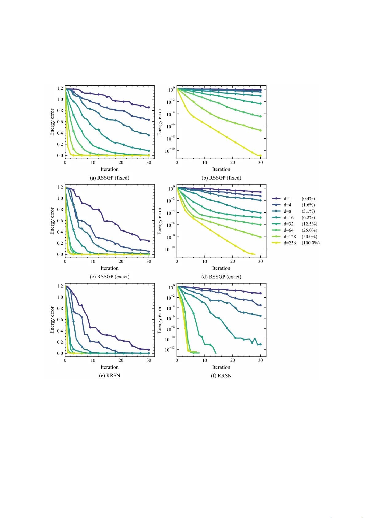
Quan tum circuit design from a retraction-based Riemannian optimization framew ork Zhijian Lai 1 , Han tao Nie 1 , Jia yuan W u 2 , Dong An 1 1 Beijing In ternational Center for Mathematical Researc h, Peking Univ ersity , Beijing 100871, China 2 Wharton Departmen t of Statistics and Data Science, Universit y of Pennsylv ania, Philadelphia, P A 19104, USA Emails: lai_zhijian@pku.edu.cn ; nht@pku.edu.cn ; jyuan w@wharton.up enn.edu ; dongan@pku.edu.cn Abstract Designing quan tum circuits for ground state preparation is a fundamental task in quan tum infor- mation science. How ev er, standard V ariational Quan tum Algorithms (VQAs) are often constrained b y limited ansatz expressivit y and diﬃcult optimization landscap es. T o address these issues, we adopt a geometric p erspective, formulating the problem as the minimization of an energy cost function di- rectly ov er the unitary group. W e establish a retraction-based Riemannian optimization framework for this setting, ensuring that all algorithmic pro cedures are implementable on quantum hardware. Within this framew ork, we unify existing randomized gradient approaches under a Riemannian Ran- dom Subspace Gradien t Pro jection (RRSGP) metho d. While recen t geometric approac hes ha ve predominan tly fo cused on such ﬁrst-order gradient descent techniques, eﬃcient second-order meth- o ds remain unexplored. T o bridge this gap, we derive explicit expressions for the Riemannian Hessian and sho w that it can b e estimated directly on quantum hardware via parameter-shift rules. Build- ing on this, we prop ose the Riemannian Random Subspace Newton (RRSN) metho d, a scalable second-order algorithm that constructs a Newton system from measurement data. Numerical sim- ulations indicate that RRSN achiev es quadratic conv ergence, yielding high-precision ground states in signiﬁcantly fewer iterations compared to b oth existing ﬁrst-order approaches and standard VQA baselines. Ultimately , this work provides a systematic foundation for applying a broader class of eﬃcien t Riemannian algorithms to quantum circuit design. Keyw ords: Quan tum circuit design; Ground state preparation; Riemannian optimization; Gradien t descent metho ds; Newton metho ds 1 In tro duction Designing quantum circuits to prepare sp eciﬁc quan tum states lies at the heart of quantum information science. This task, often framed as the ground state preparation for a given Hamiltonian, is fundamen tal to realizing the full p oten tial of quantum computing across a broad range of domains. Prominen t appli- cations include simulating electronic structures in quan tum chemistry [ 44 , 38 , 27 ], solving combinatorial optimization problems via the Quan tum Approximate Optimization Algorithm (QAO A) [ 18 , 65 ], and enabling Quantum Machine Learning (QML) tasks [ 11 , 52 ]. In the Noisy In termediate-Scale Quantum (NISQ) era [ 46 ], improving the eﬃciency and practical feasibility of such circuit designs is particularly imp ortan t. Curren tly , the dominant paradigm for addressing these problems is the V ariational Quantum Al- gorithm (V QA) framework [ 15 , 10 ], whic h relies on optimizing the Parameterized Quantum Circuits (PQCs) [ 8 ]. Throughout the pap er, we consider an N -qubit system with p := 2 N . Given an initial state ψ 0 = | ψ 0 ⟩⟨ ψ 0 | and a target Hamiltonian O , the standard VQA approach aims to solve min θ ∈ R m f ( θ ) = T r  O U ( θ ) ψ 0 U ( θ ) †  , (P1) where the structure of PQC (i.e., ansatz) U ( θ ) is ﬁxed a priori, t ypically based on heuristic designs, suc h as the hardware-eﬃcien t ansatz [ 27 ], unitary coupled-cluster ansatz [ 44 , 48 ], or Hamiltonian v ariational ansatz [ 60 , 63 ]. The parameters θ ∈ R m are optimized b y classical metho ds. This paradigm is hardware- friendly as it k eeps a constant circuit depth and uses well-established classical optimization routines. Ho wev er, the VQA framew ork faces some b ottlenec ks. First, the ﬁxed ansatz limits the expressivity of the model, b ecause the true ground state may lie outside the reachable state space generated by U ( θ ) 1 [ 53 , 22 ]. Second, the cost landscap e of ( P1 ) is often highly non-con vex and riddled with lo cal minima [ 12 ]. More critically , VQAs suﬀer from the barren plateau [ 39 , 32 ], where gradients v anish exp onen tially with the n umber of qubits, making training eﬀectively imp ossible. In ligh t of these challenges, there is gro wing interest in a geometric optimization p ersp ectiv e. The cen tral idea is to lift the restriction of a ﬁxed ansatz and instead optimize directly o ver the full space of quantum circuits. Speciﬁcally , one formulates the task as a Riemannian optimization (also called manifold optimization) problem [ 17 , 4 , 13 , 23 ]: min U ∈ U( p ) f ( U ) = T r  O U ψ 0 U †  , (P2) where the searc h space is the compact Lie group of p × p unitary matrices: U( p ) =  U ∈ C p × p   U † U = I  . (1) This set, kno wn as the unitary group 1 , is a Riemannian manifold of dimension p 2 = 4 N . By treating the circuit U itself as the v ariable on a manifold, one can use the rich geometric to ols and algorithms from Riemannian optimization. Recen tly , many w orks [ 62 , 45 , 36 , 35 , 40 ] hav e explored this geometric viewp oint. These approaches t ypically start from the Riemannian gradient ﬂow asso ciated with ( P2 ), namely , d dt U ( t ) = − grad f ( U ( t )) with U ( t ) ∈ U( p ) , and then discretize it in time, leading to the Riemannian Gradien t Descent (RGD) up date U k +1 = e − t k [ O,ψ k ] U k with U 0 = I , where the (Riemannian) gradien t term [ O , ψ k ] is the commu- tator b et ween O and ψ k , and ψ k = U k ψ 0 U † k is the current state. Ho wev er, a practical diﬃcult y of RGD is the eﬃcient implementation (or approximate simulation) of the additional gate e − t k [ O,ψ k ] . Since this gate dep ends adaptively on ψ k , realizing it typically requires rep eatedly extracting information about the current state, leading to an exp onen tial computational cost in terms of the num ber of iterations. T o address this issue, one often pro jects [ O, ψ k ] on to a c hosen subset of Pauli w ords (e.g., the set of one- and t wo-local P auli w ords) and implemen ts the resulting ev olution using a T rotter appro ximation [ 62 ]. It has also been emphasized that randomized selection of P auli words can substantially ensure the con vergence b eha vior of such schemes [ 45 ]. Indeed, it can be viewed as a randomized v ariant of RGD on the mani- fold, for which con vergence to the ground state from almost all initial states has been established [ 36 ]. A related v arian t that up dates along a single randomly chosen Pauli w ord p er iteration has also been studied [ 36 , 35 , 40 ]. The ab o ve approaches are collectively referred to as r andomize d RGD metho ds. On the other hand, the RGD up date can also b e interpreted through the lens of quantum imaginary-time ev olution [ 41 , 40 ] and double-brack et quantum algorithms [ 20 , 57 , 56 ]. Although these studies ha ve explicitly utilized Riemannian gradient descent, a comprehensive mo dern Riemannian optimization framework [ 4 , 13 , 23 ] tailored for problem ( P2 ) is still absent. As a result, the literature has predominan tly fo cused on ﬁrst-order metho ds such as RGD, while second-order Riemannian metho ds remain largely unexplored regarding their implementabilit y on quantum hardware. Moreov er, the con vergence analyses do not directly use the established Riemannian optimization theory , which mak es them problem-sp eciﬁc and hard for generalization to diﬀerent choices in the algorithm design. The mo dern Riemannian optimization framework [ 4 , 13 , 23 ] is r etr action-b ase d , where retractions [ 6 ] are the most general class of mappings that map tangen t v ectors bac k on to the manifold while still guaranteeing conv ergence. In this paper, w e dev elop a complete retraction-based framework for problem ( P2 ), in whic h ev ery algorithmic comp onent is imple men table on quantum hardw are. The main con tributions of this work can b e summarized as follows. 1. First-order metho ds. W e formalize the T rotter approximation [ 59 , 55 ] as a retraction on unitary group, thereby bridging the algorithmic design with standard optimization metho dology . W e then in terpret the randomized RGD metho ds in tro duced abov e [ 45 , 36 , 35 , 40 ] as a Riemannian R andom Subsp ac e Gr adient Pr oje ction (RRSGP) metho d: at eac h iteration, the full Riemannian gradient is randomly orthogonally pro jected onto a d = poly ( N ) -dimensional subspace of the current tangent space, and the up date is taken along the resulting pro jected gradient. F urthermore, we introduce an exact line-search technique to determine the optimal step size, whic h is equiv alen t to solving a single-parameter V QA subproblem. 2. Second-order metho ds. W e derive an explicit expression for the Riemannian Hessian (i.e., the manifold analogue of the Euclidean Hessian) of the cost function in ( P2 ). Crucially , we demon- strate that the Riemannian Hessian can b e estimated directly on quantum hardw are via quantum 1 T o simplify the description, we do not use the sp ecial unitary group SU( p ) in this pap er. In the implementation, it suﬃces to remo ve the all-identit y term from the P auli words. 2 measuremen ts using parameter-shift rules [ 37 , 51 ], just as existing studies [ 62 , 45 , 40 ] estimate the Riemannian gradient through quantum measurements. Building on this, we prop ose a fully quan tum-implementable Riemannian Newton algorithm. T o ensure scalabilit y , we adopt a ran- domized strategy analogous to RRSGP and introduce the Riemannian R andom Subsp ac e Newton (RRSN) metho d. RRSN constructs a d × d Newton system from measurement data, stabilized b y regularization techniques. Our numerical results demonstrate that RRSN ac hieves a quadratic con vergence rate, attaining the ground state in signiﬁcantly few er iterations compared to random- ized RGD and VQA baselines. W e sho w that a shallow VQA warm start eﬀectively combines the hardw are eﬃciency of PQCs with the high-accuracy reﬁnement of Riemannian optimization. Organization In Section 2 , w e review the ﬁrst-order geometry of the unitary group and in tro duce the quan tum-implementable retractions. W e then develop the ﬁrst-order algorithm framew ork, sp eciﬁcally the Riemannian Random Subspace Gradient Pro jection (RRSGP) method. Section 3 focuses on the second-order geometry and algorithms: w e derive the explicit form of the Riemannian Hessian, show ho w to estimate it via measurements, and prop ose the Riemannian Random Subspace Newton (RRSN) metho d. Section 4 presen ts numerical simulations on the Heisen b erg XXZ mo del to ev aluate the p erfor- mance of our algorithms. W e conclude in Section 5 . 2 First-order geometry and algorithms This section pro vides a minimal review of the ﬁrst-order geometry of the unitary group, follow ed by an introduction to several ﬁrst-order Riemannian algorithms for problem ( P2 ) that can b e implemented on quan tum hardware. F or a complete and rigorous deriv ation of geometry , w e refer the reader to the monographs [ 4 , 13 ]. Second-order geometry and algorithms will b e presented in the next section. Throughout the pap er, we set p = 2 N for an N -qubit system. 2.1 First-order geometry First, we review the fundamental geometric concepts and to ols required for optimization on the unitary group. 2.1.1 T angen t space and orthogonal pro jection The tangent space of a manifold at a given p oin t consists of all directions in whic h one can mov e from that p oin t. F or the unitary group U( p ) , this space admits an explicit description in terms of skew-Hermitian matrices. F or any U ∈ U( p ) , the tangent space at U is given by T U = { Ω U : Ω † = − Ω } = u ( p ) U, (2) where u ( p ) =  Ω ∈ C p × p : Ω † = − Ω  is the Lie algebra of U( p ) . This Lie algebra is a real vector space consisting of all skew-Hermitian p × p matrices and is closed under the Lie brack et [ X , Y ] = X Y − Y X . In particular, at the identit y I ∈ U( p ) , one has T I = u ( p ) ; since dim u ( p ) = p 2 , the manifold U( p ) has dimension p 2 . W e equip the ambien t space C p × p ⊇ U( p ) with the real F rob enius inner pro duct ⟨ A, B ⟩ = ℜ T r( A † B ) . With respect to this inner product, the normal space at U ∈ U( p ) is giv en by N U =  N ∈ C p × p : ⟨ N , X ⟩ = 0 , ∀ X ∈ T U  = { H U : H † = H } = H ( p ) U, where H ( p ) denotes the space of Hermitian p × p matrices. Using the orthogonal decomposition C p × p = T U ⊕ N U , one obtains the orthogonal pro jection of an y Z ∈ C p × p on to the tangent space T U : P U ( Z ) := Skew( Z U † ) U, with Sk ew ( A ) := 1 2 ( A − A † ) . (3) 2.1.2 Riemannian gradient W e regard U( p ) as a Riemannian submanifold of C p × p b y equipping each tangent space T U with the R iemannian metric (some inner pro duct) ⟨ X , Y ⟩ U ≡ ⟨ X, Y ⟩ = ⟨ e X , e Y ⟩ = T r( e X † e Y ) for all X , Y ∈ T U , where e X , e Y ∈ u ( p ) are the left skew-Hermitian representations, deﬁned through X = e X U , Y = e Y U . 3 (a) (b) Figure 1: The geometric illustration of Riemannian gradient and Riemannian algorithm iterations. (a) F or the sake of demonstration, we imagine the curved space U( p ) as a sphere. Giv en a p oin t U on U( p ) , the tangen t space T U is similar to the tangent plane at that p oin t. W e plot the con tours (dash lines) of the cost function f on U( p ) , where the Riemannian gradient grad f ( U ) is a sp ecial v ector in the tangen t plane. This vector is orthogonal to the contour and p oints in the direction of the fastest increase of f . (b) The iteration pro cess of a t ypical Riemannian optimization algorithm U k +1 = R U k ( t k η k ) , which is an extension of iteration x k +1 = x k + t k η k in Euclidean space. With this metric, the Riemannian gradient of an y smo oth function f : U( p ) ⊆ C p × p → R can b e computed b y (see [ 13 , Prop osition 3.61]) grad f ( U ) = P U  ∇ f ( U )  ∈ T U , (4) where ∇ f ( U ) ∈ C p × p is the usual gradient. At a p oin t U , the Riemannian gradient grad f ( U ) is the tangen t v ector of steep est ascent of f and th us forms a basic comp onen t of Riemannian optimization algorithms; see (a) in Figure 1 . F or our cost f ( U ) = T r  O U ψ 0 U †  in ( P2 ), the Euclidean gradient is ∇ f ( U ) = 2 O U ψ 0 . In general, when A and B are (sk ew-)Hermitian, then Sk ew (2 AB ) = [ A, B ] (5) holds. Applying the ab ov e with A := O and B := U ψ 0 U † , and in voking Eq. ( 4 ), we obtain grad f ( U ) = Sk ew (2 OU ψ 0 U † ) U = [ O, U ψ 0 U † ] U ∈ T U , (6) where the commutator g grad f ( U ) := [ O , U ψ 0 U † ] ∈ u ( p ) serves as the left skew-Hermitian representation of grad f ( U ) . 2.1.3 Quan tum-implementable retractions R etr actions [ 6 , 4 ] provide a principled w ay to mo ve along tangen t directions while ensuring that iterates remain on the manifold, and they constitute a central step of Riemannian optimization theory . Deﬁne the tangen t bundle T U( p ) := { ( U, η ) : U ∈ U( p ) , η ∈ T U } . A retraction on U( p ) is a smo oth map R : T U( p ) → U( p ) , ( U, η ) 7→ R U ( η ) , such that for any U ∈ U( p ) and η ∈ T U , the induced curve t 7→ γ ( t ) := R U ( tη ) satisﬁes γ (0) = U and ˙ γ (0) = η . (7) The ab o ve conditions are the key to ensuring conv ergence of the Riemannian algorithm, rather than the sp eciﬁc form of the retraction. W e denote by R U the restriction of R to T U . Once a retraction is ﬁxed, the next iterate U k +1 is obtained by selecting a tangent direction η k ∈ T U k at the current iterate U k and mo ving along the curve t 7→ R U k ( tη k ) with an appropriate step size t k ; see (b) in Figure 1 . This mec hanism forms the core up date rule of Riemannian optimization, whose details will b e presented in Section 2.2 . Below, we discuss tw o retractions on U( p ) that are implementable on quan tum hardware. Riemannian Exponential map F or an y U ∈ U( p ) , the (Riemannian) Exp onential map Exp U : T U → U( p ) is giv en by Exp U ( η ) = exp  e η  U, (8) 4 where we often use the sym b ol tilde to denote the left sk ew-Hermitian represen tation of the tangent v ector in T U , i.e., η = ˜ η U with ˜ η ∈ u ( p ) . Consider the curve γ ( t ) := Exp U ( tη ) = exp( t e η ) U. (9) It is straightforw ard to v erify that γ (0) = U , and ˙ γ (0) = e η exp( t e η ) U | t =0 = η . Therefore, the Exponential map serv es as a v alid retraction. The Exp onen tial map is a fundamen tal concept in diﬀerential geometry [ 33 ]; the curve it induces in Eq. ( 9 ) pro vides the intrinsic analogue of a straigh t line on a manifold, namely , a geo desic. On the other hand, w e use exp( · ) or e ( · ) for the ordinary matrix exp onen tial, whic h should b e distinguished from Exp. In general, the Exp onen tial map on a manifold do es not alwa ys inv olv e a matrix exp onential. F or instance, on the trivial manifold R n , the Exponential map takes the simple form Exp x ( η ) = x + η for x ∈ R n and η ∈ T x ≡ R n . In fact, the Exp onen tial map is seldom used in Riemannian optimization due to its high compu- tational cost on classical computers. F or our manifold U( p ) , more eﬃcient alternatives (such as the Ca yley transform retraction [ 61 ], QR-based retraction [ 50 , 4 ], or p olar decomp osition [ 5 , 4 ]) are typically preferred. Ho wev er, the curv e in Eq. ( 9 ) is particularly w ell suited for implementing iterative up dates in quantum circuits b ecause exp( t e η ) = exp( − it · i e η ) constitutes a standard quan tum gate, with the step size t serving as the rotation angle and i e η acting as the Hermitian generator. T rotter retraction The well-kno wn ﬁrst-order T rotter approximation [ 59 , 34 ] also induces a v alid retraction. Let P N = { P j } 4 N j =1 denote the N -qubit Pauli words, where P j = N N ℓ =1 σ j ℓ with σ j ℓ ∈ { I , X , Y , Z } . Then i P N = { iP j } is an orthogonal (non-normalized) basis of Lie algebra u ( p ) . F or an y U ∈ U( p ) and η ∈ T U , write η = ˜ η U with ˜ η ∈ u ( p ) , and expand ˜ η in the Pauli basis: ˜ η = 4 N X j =1 iω j P j , ω j = ⟨ ˜ η, iP j ⟩ ⟨ iP j , iP j ⟩ = − i 2 N T r( ˜ ηP j ) . (10) The T r otter r etr action T rt U : T U → U( p ) is deﬁned by T rt U ( η ) =   4 N Y j =1 exp  iω j P j    U. (11) Consider the curv e γ ( t ) := T rt U ( tη ) =   4 N Y j =1 exp  iω j P j t    U ≡ A ( t ) U. (12) It is immediate that γ (0) = U . Applying the pro duct rule yields ˙ A ( t ) = 4 N X k =1   Y j k exp( iω j P j t )   . (13) Ev aluating at t = 0 , w e obtain ˙ γ (0) = ˙ A (0) U =  P 4 N k =1 iω k P k  U = η . Hence, T rt U is a v alid retraction. Ob viously , this retraction stems from the ﬁrst-order T rotter approximation: exp ( t e η ) = exp   4 N X j =1 iω j P j t   = 4 N Y j =1 exp  iω j P j t  + O ( t 2 ) . (14) The same idea extends naturally to the second-order [ 54 ] and higher-order T rotter sc hemes [ 55 ], pro ducing T rotter-lik e retractions that more closely approximate the geo desic t 7→ exp( t ˜ η ) . How ever, this reﬁne- men t is unnecessary , since the ﬁrst-order construction in Eq. ( 11 ) already pro vides suﬃcient conv ergent prop erties, b oth in our theoretical analysis and in numerical exp eriments for Riemannian optimization. W e refer to the t wo retractions deﬁned ab ov e, Exp and T rt , as quantum-implementable r etr actions b ecause they b oth tak e the form of a standard quantum gate. In contrast, man y other retractions on the unitary group do not admit such ph ysical implementations. F or example, the Ca yley transform retraction [ 61 ] requires matrix inv ersion, while the QR-based retraction [ 50 , 4 ] and p olar decomp osition [ 5 , 4 ] retraction rely on matrix factorizations. These pro cedures cannot b e executed directly on quantum hardw are. One may say that the developmen t of quantum computing has brough t renewed attention to certain mathematical ob jects that were previously ov erlo ok ed by classical computation. 5 2.2 First-order algorithms In this subsection, we ﬁrst review the general framework of Riemannian optimization and then discuss the simplest ﬁrst-order metho d, the Riemannian Gradien t Descent (RGD). Ho wev er, implemen ting RGD on quan tum hardw are can suﬀer from the curse of dimensionality . T o address this, w e consider a v ariant that pro jects the Riemannian gradient onto a randomly low-dimensional subspace, namely the Riemannian Random Subspace Gradien t Pro jection (RRSGP). Finally , we also consider employing exact line-search to accelerate conv ergence. Our guiding principle is to ensure full consistency b et ween circuit implemen tation and optimization framew ork, while using optimization techniques to enhance circuit design. 2.2.1 General Riemannian algorithm framework In the Euclidean case, minimizing f : R n → R often amounts to generating a sequence { x k } via up dates of the form x k +1 = x k + t k η k , where η k ∈ R n is a searc h direction (e.g., negative gradient or Newton direction) and t k > 0 is a step size, chosen as a ﬁxed constant [ 42 ] or b y a line-search strategy such as Armijo bac ktracking [ 43 ], exact line-search [ 43 ], or Barzilai-Borwein rule [ 47 ]. On the U( p ) , this idea is adapted by replacing straight-line steps with mov es along tangen t directions follo wed by a retraction bac k onto the manifold. Giv en an initial p oin t U 0 ∈ U( p ) , a Riemannian algorithm generates { U k } ⊆ U( p ) by U k +1 = R U k ( t k η k ) , k = 0 , 1 , . . . , (15) where η k ∈ T U k is a tangent vector in the current tangen t space (e.g., the negative Riemannian gradient in Eq. ( 6 ), or the Riemannian Newton direction to b e in tro duced in Section 3 ), and R U k : T U k → U( p ) is a retraction at U k , such as the Exp onential map Exp or the T rotter retraction T rt in tro duced previously; see (b) in Figure 1 . By c ho osing η k and t k in analogy with their Euclidean coun terparts (e.g., Riemannian gradient descent [ 17 , 14 ], Riemannian conjugate gradien t [ 49 , 1 ], Riemannian Newton [ 4 , 19 ], or Riemannian Barzilai-Borw ein [ 26 ]), one obtains Riemannian algorithms that inherit the corresp onding con vergence guarantees from the Euclidean setting. Eq. ( 15 ) also serv es as a prerequisite for the second- order algorithms in Section 3 later. 2.2.2 Riemannian gradient descent (R GD) W e b egin by considering the simplest metho d, namely Riemannian Gradient Descent (R GD) metho d with the Exp onen tial map R = Exp for problem ( P2 ). Its up date rule is U k +1 = Exp U k ( − t k grad f ( U k )) = exp ( t k [ ψ k , O ]) U k , k = 0 , 1 , . . . , (16) where step size t k > 0 , ψ k := U k ψ 0 U † k denotes the intermediate quan tum state at iteration k , and − g grad f ( U k ) = [ ψ k , O ] ∈ u ( p ) . Setting the initial gate to U 0 = I (as we do throughout this pap er), the resulting quan tum state | ψ T ⟩ = U T | ψ 0 ⟩ after T up dates is giv en by | ψ T ⟩ = exp ( t T − 1 [ ψ T − 1 , O ]) · · · exp ( t 1 [ ψ 1 , O ]) exp ( t 0 [ ψ 0 , O ]) | ψ 0 ⟩ . (17) The o verall plan op erates as follows: information ob tained from the state generated by the current circuit is used to select additional gates that, when app ended, drive the circuit output closer to the ground state. This pro cedure is applied iterativ ely , yielding a progressively reﬁned circuit. In contrast to traditional V QAs, whose ansatz is ﬁxed in adv ance, the circuit architecture here ev olves dynamically during the optimization pro cess. Suc h dynamical arc hitectures are referred to as adaptive circuits, for example, A daptVQE [ 21 , 58 ]. The key challenge no w is to implemen t the up date gates exp  t k [ ψ k , O ]  on circuits. Although one can realize this via v arious Hamiltonian simulation techniques, here we instead employ the T rotter retraction R = T rt , whose quantum implemen tation is sim pler than that of R = Exp . F rom the standp oin t of con vergence, employing the T rotter retraction still provides the guarantees we require, since it satisﬁes conditions Eq. ( 7 ). Consequently , using the T rotter retraction, the RGD up date takes the form U k +1 = T rt U k  − t k grad f ( U k )  =   4 N Y j =1 exp  iω j k P j t k    U k , k = 0 , 1 , . . . , (18) 6 where − g grad f ( U k ) = [ ψ k , O ] ∈ u ( p ) admits the Pauli expansion (see Eq. ( 10 )): [ ψ k , O ] = 4 N X j =1 iω j k P j , ω j k := − i 2 N T r  [ ψ k , O ] P j  = − 1 2 N i T r  ψ k [ O , P j ]  ∈ R , (19) where the last equalit y follows from T r([ A, B ] C ) = T r( A [ B , C ]) . In fact, we can determine the v alue of ω j k b y measuremen ts on the current state ψ k . T o this end, w e require the following lemma; its pro of is provided in A . (F or the momen t, w e ignore the exp onen tial term 4 N and fo cus on the exact algorithmic formulation.) Lemma 1 (Gradient co eﬃcien t estimation) . Given any pur e density op er ator ψ , any Hamiltonian O , and any Hermitian gener ator P , c onsider the exp e ctation value on a variational cir cuit w.r.t. a single r e al p ar ameter x , i.e., g ( x ) = T r { OU ( x ) ψ U ( x ) † } , (20) wher e U ( x ) = e ixP / 2 . Then, g ′ (0) = i 2 T r { ψ [ O, P ] } . Mor e over, if P 2 = I , then by the p ar ameter-shift rule [ 37 , Eq. (9)], one has g ′ (0) = 1 2 h g  π 2  − g  − π 2 i . (21) T o estimate the co eﬃcien ts ω j k in Eq. ( 18 ), w e consider the following PQC cost function: g j k ( x ) := T r { O U ( x ) ψ k U ( x ) † } , U ( x ) = e ixP j / 2 . (22) Since P j is a P auli word, by Lemma 1 and Eq. ( 19 ), we obtain ω j k = 1 2 N h g j k  − π 2  − g j k  π 2 i . (23) Th us, ω j k can b e directly estimated on a quantum device. F or an y P auli word P j and any real ev olution time ω j k t k , the corresp onding unitary exp( iP j · ( ω j k t k )) can b e synthesized using standard Hamiltonian sim ulation techniques. In this work, we adopt s uc h Pauli-ev olution gates as fundamental building blo c ks. Consequen tly , ignoring the exp onential scaling 4 N , the standard RGD with the T rotter retraction can b e implemen ted entirely using quantum circuits, ac hieving a seamless uniﬁcation of quan tum imple- men tation and optimization framework. 2.2.3 Riemannian random subspace gradient pro jection (RRSGP) Since the T rotter up date in Eq. ( 18 ) demands exponentially many gates p er iteration, whic h is clearly impractical, a simple remedy is to choose a m uch smaller subset of d Pauli words at random from the full set of 4 N . The up date then b ecomes U k +1 =   Y j ∈ S k exp  iω j k P j t k    U k , k = 0 , 1 , . . . , (24) where S k ⊆ { 1 , 2 , . . . , 4 N } is a random subset of size d = p oly( N ) . Each co eﬃcien t ω j k is computed as Eq. ( 23 ), and this pro cedure adds only d gates p er up date. In fact, we are not introducing a new retraction here, but rather a Riemannian analogue of Random Subspace Gradien t Pro jection (RSGP) metho d. Let us review RSGP in the Euclidean setting. T o solv e min x ∈ R n f ( x ) with very large n , one pro jects the full gradient on to a random d -dimensional subspace U k ⊆ R n ( d ≪ n ) and then takes a descent step within that subspace. Concretely , the RSGP up date is x k +1 = x k + t k Π k  −∇ f ( x k )  , (25) where Π k ∈ R n × n is the orthogonal pro jector onto U k . Equiv alen tly , one often writes Π k = P k P ⊤ k , where P k ∈ R n × d is a random matrix satisfying P ⊤ k P k = I d and E  P k P ⊤ k  = d n I n . This RSGP approach preserv es conv ergence guarantees in exp ectation, comparable to those of full gradient descent [ 29 , 30 ]. In the Riemannian context, we will orthogonally pro ject the full Riemannian gradient grad f ( U k ) ∈ T U k on to a random d -dimensional subspace of the current tangent space T U k . Since eac h tangent space 7 T U k = u ( p ) U k is isomorphic to the Lie algebra u ( p ) , it suﬃces to pro ject the sk ew-Hermitian part g grad f ( U k ) = P 4 N j =1 iω j k P j ∈ u ( p ) onto a random d -dimensional subspace of u ( p ) . Concretely , we sample d Pauli words from the full basis { iP j } , and let the selected index set b e S k ⊆ { 1 , 2 , . . . , 4 N } . W e use S k ⊆ T U k to denote the subspace spanned b y these selected directions. The pro jected gradient is then ζ k := Pro j S k ( − grad f ( U k )) =   X j ∈ S k iω j k P j   U k ∈ S k . (26) Substituting ζ k in to the T rotter retraction U k +1 = T rt U k ( t k ζ k ) exactly recov ers the up date in Eq. ( 24 ). The complete RRSGP pro cedure is summarized in Algorithm 1 . Algorithm 1 Riemannian Random Subspace Gradient Pro jection (RRSGP) Metho d for ( P2 ) Input: N -qubits system, Hamiltonian O , initial state ψ 0 , subspace dimension d = p oly( N ) . P auli set P N = { P j } 4 N j =1 with P j = N N ℓ =1 σ j ℓ , σ j ℓ ∈ { I , X, Y , Z } . 1: for k = 0 , 1 , . . . do 2: Step 1: Subspace Sampling 3: Uniformly sample index set S k ⊆ { 1 , . . . , 4 N } of size d . 4: Step 2: Gradien t Estimation on Subspace ▷ − g grad f ( U k ) 5: for j ∈ S k do 6: Deﬁne g j k ( x ) = T r { O e ixP j / 2 ψ k e − ixP j / 2 } . 7: Set ω j k = 1 2 N [ g j k ( − π 2 ) − g j k ( π 2 )] . ▷ By parameter-shift. 8: end for 9: Step 3: Step Size Selection 10: Cho ose a step size t k . ▷ Fixed step (e.g., 0 . 1 ) or exact line-search. 11: App end up date gates | ψ k +1 ⟩ ← Q j ∈ S k exp( iω j k P j t k ) | ψ k ⟩ . 12: Set k ← k + 1 . 13: end for The uniform random selection of a new subspace at eac h iteration is critical to preserve con vergence of RRSGP . F or instance, the metho d in [ 62 ] employs a structure similar to Algorithm 1 but restricts optimization to a ﬁxed subspace (e.g., the one-lo cal or t wo-local Pauli set); consequently , the theoretical con vergence guarantees no longer hold. More recen tly , [ 45 ] improv ed upon this b y adopting a randomized subspace of p olynomial dimension, yielding an algorithm that is equiv alen t to Algorithm 1 . A dditionally , v arian ts corresp onding to the subspace dimension d = 1 ha ve b een inv estigated in [ 36 , 35 , 40 ]. How- ev er, we formalize this pro cedure within a retraction-based optimization framework. This p erspective clariﬁes that a broad range of optimization techniques can b e easily incorp orated into Algorithm 1 to enhance eﬃciency (e.g., the exact line-searc h rule detailed in the next subsection). Moreo ver, within this framework, the conv ergence prop erties of the algorithm can b e established b y using standard results from Riemannian optimization theory . 2.2.4 Exact line-search for RRSGP In a quan tum implemen tation of Algorithm 1 , running T iterations yields a circuit with T d Pauli- ev olution gates, so each additional iteration directly increases circuit depth. Therefore, to keep the circuit shallow, it is crucial to reduce total T by selecting step size t k carefully at every iteration, rather than using a constant is common in deep learning ﬁeld. W e now introduce an exact line-searc h pro cedure for choosing the step size t k in Step 3 of Algorithm 1 . Giv en the pro jected gradien t ζ k in Eq. ( 26 ), the exact line-searc h is deﬁned as t k := arg min t> 0 ϕ ( t ) = f (T rt U k ( tζ k )) = f   Y j ∈ S k exp  iω j k P j t  U k   = T r  O V ( t ) ψ k V ( t ) †  , (27) where V ( t ) := Q j ∈ S k exp( iω j k P j t ) . This choice guarantees the maximal decrease of the cost along the pro jected searc h direction ζ k at each iteration, thereby he lping reduce the total num b er of iterations. 8 The trade-oﬀ is that each iteration no w requires (approximately) solving an auxiliary one dimensional subproblem min t> 0 ϕ ( t ) , whic h is equiv alent to training a single parameter PQC. In our numerical ex- p erimen ts, we use the A dam optimizer [ 28 ] to solv e this subproblem, and the results s ho w that it can eﬀectiv ely reduce the iteration count T . 3 Second-order geometry and algorithms So far, we fo cused on ﬁrst-order Riemannian algorithms for solving problem ( P2 ). A natural question is whether the second-order algorithms can also b e implemented on quantum circuits. It is well known that the Newton metho d [ 16 ] ac hieves quadratic conv ergence when initialized suﬃciently close to the optim um. Hence, applying a Riemannian Newton metho d [ 19 , 4 ] has the p oten tial to reach the solution in far few er iterations, thereby producing shallo wer circuits. In th is section, we discuss how to realize the Riemannian Newton metho d for solving problem ( P2 ). The ﬁrst requiremen t is the ability to compute the k ey second-order geometric ob ject, namely , the Riemannian Hessian op erator. 3.1 Second-order geometry In the Euclidean setting, given a smo oth function f : R n → R , the Hessian ∇ 2 f ( x ) at x ∈ R n is an n × n real symmetric matrix. Equiv alen tly , it can b e viewed as a self-adjoint linear op erator on R n . As a natural extension, the Riemannian Hessian of f at a p oint on a manifold is a self-adjoint linear op erator acting on the tangent space at that p oin t. The Riemannian Hessian characterizes the second- order v ariation of the cost function f along tangent directions. It pro vides the curv ature information to construct second-order optimization algorithms [ 3 , 13 ], that can accelerate the conv ergence. In the next prop osition, w e presen t an explicit expression for the Riemannian Hessian of our cost function in problem ( P2 ), whose pro of is provided in B.1 . Prop osition 1 (Riemannian Hessian) . F or the c ost function f : U( p ) → R deﬁne d by f ( U ) = T r  O U ψ 0 U †  , the Riemannian Hessian of f at U ∈ U( p ) is the self-adjoint line ar op er ator Hess f ( U ) : T U → T U given by Hess f ( U )[Ω U ] = 1 2 ([ O , [Ω , ψ ]] + [[ O , Ω] , ψ ]) U, (28) wher e ψ := U ψ 0 U † and T U = { Ω U : Ω ∈ u ( p ) } . Identifying T U ≃ u ( p ) yields the asso ciate d op er ator g Hess f ( U ) : u ( p ) → u ( p ) , g Hess f ( U )[Ω] = 1 2 ([ O , [Ω , ψ ]] + [[ O , Ω] , ψ ]) , (29) which is self-adjoint on the Lie algebr a u ( p ) . Her e, “self-adjoint” is understo o d with r esp e ct to the F r ob e- nius inner pr o duct ⟨ A, B ⟩ = T r  A † B  . Indeed, for any U ∈ U( p ) and X ∈ C p × p , the Riemannian Hessian g Hess f ( U ) satisﬁes g Hess f ( U )  X †  = ( g Hess f ( U )[ X ]) † and g Hess f ( U )[ i X ] = i g Hess f ( U )[ X ] . Its linearity and self-adjointness are straigh tforward to v erify . Pro ofs of these prop erties can b e found in B.2 . 3.2 Second-order algorithms In this section, w e ﬁrst in tro duce a standard Riemannian Newton metho d and then prop ose a random subspace v arian t for the practical implementation. 3.2.1 Riemannian Newton The Riemannian Newton method also ﬁts within the general up date framew ork U k +1 = R U k ( t k η k ) in Eq. ( 15 ). The key distinction is that the searc h direction η k = e η k U k ∈ T U k is now c hosen as the Newton direction. Riemannian Newton equation At the iteration k , the Newton direction e η k = Ω N k ∈ u ( p ) is deﬁned as the solution to the follo wing (Riemannian) Newton equation: Hess f ( U k )[Ω N k U k ] = − grad f ( U k ) , (30) 9 whic h constitutes a linear system on the current tangent space T U k . Dropping the rightmost factor U k , the ab o ve equation can b e equiv alently written on the Lie algebra u ( p ) as g Hess f ( U k )[Ω N k ] = − g grad f ( U k ) , (31) F or con venience, let ψ k = U k ψ 0 U † k and deﬁne L k (Ω) ≜ g Hess f ( U k )[Ω] = 1 2 ([ O , [Ω , ψ k ]] + [[ O , Ω] , ψ k ]) . (32) Then the Newton direction e η k = Ω N k ∈ u ( p ) is obtained by solving L k (Ω N k ) = [ ψ k , O ] . (33) The Riemannian Newton up date is giv en by U k +1 = R U k (Ω N k U k ) with unit step size t k ≡ 1 . W e emphasize that the use of a constan t unit step size is imp ortant for achieving quadratic conv ergence. Solving Newton equation T o solv e the Newton equation Eq. ( 33 ), we consider the matrix represen- tation L k ∈ R 4 N × 4 N of the op erator L k with resp ect to the orthogonal basis { iP j } of u ( p ) . Speciﬁcally , for all r , s = 1 , . . . , 4 N , w e hav e ( L k ) rs = ⟨ iP r , L k ( iP s ) ⟩ = T r { ( iP r ) † L k ( iP s ) } = T r { P r L k ( P s ) } (34) = 1 2 T r { P r [ O , [ P s , ψ k ]] } + 1 2 T r { P r [[ O , P s ] , ψ k ] } (35) = 1 2 T r { ψ k [[ P r , O ] , P s ] } + 1 2 T r { ψ k [[ P s , O ] , P r ] } . (36) Under the same basis, let g k ∈ R 4 N denote the vector representation of the right-hand side of Eq. ( 33 ), i.e., negativ e Riemannian gradient. F or j = 1 , . . . , 4 N , its en tries are given by ( g k ) j = ⟨ iP j , − g grad f ( U k ) ⟩ (37) = ⟨ iP j , [ ψ k , O ] ⟩ = T r {  iP j  † [ ψ k , O ] } = − i T r { ψ k  O , P j  } . (38) W e then classically solv e the linear equation L k Ω N k = g k , (39) to obtain Ω N k ∈ R 4 N . The corresp onding Newton direction in u ( p ) is recov ered as Ω N k = 4 N X j =1 ( Ω N k ) j · iP j ∈ u ( p ) . (40) Finally , by applying the T rotter retraction R = T rt in Eq. ( 11 ), the Riemannian Newton update takes the form U k +1 = T rt U k (Ω N k U k ) =   4 N Y j =1 exp  i ( Ω N k ) j P j    U k . (41) Ev aluation of co eﬃcien ts The remaining task inv olv es the computation of g k and L k . The ev aluation of the entries ( g k ) j in Eq. ( 37 ) follows the same pro cedure as that used for computing the gradien t co eﬃcien ts in Algorithm 1 . W e consider the following univ ariate PQC cost function: g j k ( x ) := T r { O U ( x ) ψ k U ( x ) † } , U ( x ) = e ixP j / 2 . (42) By Lemma 1 , w e obtain ( g k ) j = h g j k  − π 2  − g j k  π 2 i . (43) Moreo ver, we establish the following key lemma, which shows that the matrix representation of the Hessian op erator can also b e obtained through quantum circuit measurements, in complete analogy with the gradien t. The pro ofs are deferred to A . 10 Lemma 2 (Hessian coeﬃcient estimation) . Given any pur e density op er ator ψ , any Hamiltonian O , and any Hermitian gener ators P and Q , c onsider the exp e ctation value on a variational cir cuit w.r.t. two r e al p ar ameters x, y , i.e., g ( x, y ) = T r  O W ( y ) U ( x ) ψ U ( x ) † W ( y ) †  , (44) wher e U ( x ) = e ixP / 2 and W ( y ) = e iy Q/ 2 . Then, we obtain the fol lowing r esults c onc erning the se c ond- or der p artial derivatives: g xx (0 , 0) = 1 4 T r  ψ [[ P, O ] , P ]  , g xy (0 , 0) = 1 4 T r  ψ [[ Q, O ] , P ]  . (45) Mor e over, if P 2 = Q 2 = I , then by the p ar ameter-shift rule [ 37 , Eq. (11) & Eq. (13)], one has g xx (0 , 0) = 1 2 h g  π 2 , 0  + g  − π 2 , 0  − 2 g (0 , 0) i , (46) g xy (0 , 0) = 1 4 h g  π 2 , π 2  − g  π 2 , − π 2  − g  − π 2 , π 2  + g  − π 2 , − π 2 i . (47) Note that if we aim to c ompute T r  ψ [[ P, O ] , Q ]  , it suﬃc es to swap the or der of the p ar ameterize d unitaries U ( x ) and W ( y ) in cir cuits. T o estimate the co eﬃcients ( L k ) rs in Eq. ( 36 ), w e consider the follo wing biv ariate PQC cost functions: g rs k ( x, y ) := T r  O W ( y ) U ( x ) ψ k U ( x ) † W ( y ) †  , (48) U ( x ) = e ixP s / 2 , W ( y ) = e iy P r / 2 , (49) and g sr k ( x, y ) , deﬁned analogously by exchanging the roles of P r and P s . Since b oth P r , P s are Pauli w ords, applying Eq. ( 47 ) of Lemma 2 yields ( L k ) rs = 1 2 T r { ψ k [[ P r , O ] , P s ] } + 1 2 T r { ψ k [[ P s , O ] , P r ] } (50) = 1 2 h g rs k  π 2 , π 2  − g rs k  π 2 , − π 2  − g rs k  − π 2 , π 2  + g rs k  − π 2 , − π 2 i + 1 2 h g sr k  π 2 , π 2  − g sr k  π 2 , − π 2  − g sr k  − π 2 , π 2  + g sr k  − π 2 , − π 2 i . (51) When P r and P s comm ute (which o ccurs for half of all Pauli-w ord pairs), w e hav e g rs k ( x, y ) ≡ g ( k ) sr ( x, y ) , and the expression ab o ve simpliﬁes to ( L k ) rs = h g rs k  π 2 , π 2  − g rs k  π 2 , − π 2  − g rs k  − π 2 , π 2  + g rs k  − π 2 , − π 2 i . (52) In particular, for the diagonal en tries ( L k ) j j = T r { ψ k [[ P j , O ] , P j ] } , w e consider the same PQC function g j k ( x ) deﬁned in Eq. ( 42 ). Applying Eq. ( 46 ) of Lemma 2 yields ( L k ) j j = 2 h g j k  π 2  + g j k  − π 2  − g j k (0) i . (53) Note that g j k (0) corresponds to the curren t cost v alue f ( U k ) and is indep enden t of P j ; moreo ver, the v alues g j k  ± π 2  ha ve already b een computed in Eq. ( 43 ). Therefore, the calculation of diagonal comp onen ts do es not require any additional costs. A t this p oint, we hav e completed all the comp onen ts required to implemen t the standard Riemannian Newton metho d on quantum circuits. 3.2.2 Riemannian Random Subspace Newton (RRSN) F rom the p ersp ectiv e of quan tum circuit implemen tation, Riemannian gradient descent and Riemannian Newton diﬀer only in ho w they compute the coeﬃcients (i.e., angles) of the gates. In terms of con vergence rate, the gradient descent method is at b est linearly con vergen t, whereas the Newton metho d enjo ys the w ell-known quadratic con vergence, meaning it can often reach highly accurate solutions in far fewer iterations. Ho wev er, the standard Newton metho d faces a ma jor computational b ottlenec k in terms of quan tum circuit ev aluation cost. F or an N -qubit system, forming the full Hessian matrix L k ∈ R 4 N × 4 N requires on the order of O (16 N ) ev aluations. T o ov ercome it, we prop ose the Riemannian Random Subspace Newton (RRSN) metho d. Its core idea is essentially the same as that of the previously introduced RRSGP 11 in Section 2.2.3 : at eac h iteration, we randomly select only d = p oly( N ) Pauli w ords out of the full set of 4 N , while keeping the rest of the pro cedure unchanged. The RRSN algorithm is summarized in Algorithm 2 . Under this random subspace restriction, the Newton equation L k Ω N k = g k ∈ R d (54) reduces to a d × d linear system. Uniformly sampling d Pauli basis considerably low ers the problem dimension, y et still preserves conv ergence in exp ectation, following the same rationale as RRSGP . In Algorithm 2 , w e additionally incorporate tw o standard engineering tec hniques for Newton methods: (Step 4) Hessian regularization via a p ositiv e deﬁnite mo diﬁcation and (Step 5) an Armijo bac ktracking line-searc h. Hessian regularization In the preceding discussion, we implicitly assumed that the Newton equation Eq. ( 54 ) admits a solution. How ever, this need not hold in general. Therefore, we introduce a regular- ization term δ k I d to ensure that the Hessian matrix L k ∈ R d × d b ecomes p ositiv e deﬁnite, and hence in vertible. Sp eciﬁcally , w e set δ k = max { 0 , ρ − λ min ( L k ) } , (55) for a small ρ > 0 , and λ min ( L k ) denotes the smallest eigen v alue of L k . The mo diﬁed Hessian is then e L k := L k + δ k I d ⪰ ρ I d ≻ 0 . (56) Consequen tly , the (regularized) Newton equation e L k Ω N k = g k admits a unique solution Ω N k = e L − 1 k g k ∈ R d . The corresp onding Newton direction in the chosen random subspace is then recov ered as Ω N k := X j ∈ S k ( Ω N k ) j · iP j ∈ span R  iP j : j ∈ S k  ⊆ u ( p ) . (57) Moreo ver, in this case, Newton direction Ω N k U k ∈ T U k is a descen t direction, i.e., it forms an obtuse angle with the Riemannian gradien t in the tangent space T U k . Indeed, by Eqs. ( 37 ) and ( 57 ),  grad f ( U k ) , Ω N k U k  U k = D g grad f ( U k ) , Ω N k E = X j ∈ S k ( Ω N k ) j D g grad f ( U k ) , iP j E (58) = − X j ∈ S k ( Ω N k ) j ( g k ) j = − g ⊤ k Ω N k = − g ⊤ k e L − 1 k g k < 0 , (59) where the last inequalit y holds whenever g k  = 0 . Remark 1. If g k ≈ 0 , i.e., ( g k ) j = ⟨ iP j , − g grad f ( U k ) ⟩ ≈ 0 , then the comp onents of the Riemannian gradien t along the sampled subspace are nearly zero. This situation can arise for tw o distinct reasons. First, the iterate may already b e suﬃcien tly close to an optim um, in which case the full Riemannian gradien t itself is close to zero and the algorithm should terminate. Second, the randomly chosen subspace ma y be uninformative, so that the pro jection nearly annihilates the gradien t ev en though the full gradien t remains non-negligible; in this case, the subspace should b e resampled. This phenomenon is esp ecially pronounced when d is very small (e.g., d = 1 ), since the subspace then captures only a limited amount of gradien t information. Armijo backtrac king line-search Finally , we p erform Armijo backtrac king along the Newton direc- tion. W e ﬁrst take the full step t k ← 1 and chec k whether the following Armijo c ondition holds: f  T rt U k  t k Ω N k U k  ≤ f ( U k ) + c t k  grad f ( U k ) , Ω N k U k  . (60) If not, we shrink t k ← β t k (t ypically β = 0 . 5 , c = 10 − 4 ) and rep eat the test until the ab ov e is satisﬁed. Since Ω N k U k is a descen t direction sho wn in Eq. ( 59 ), this pro cedure te rminates after ﬁnitely man y lo ops; see [ 43 , Lemma 3.1]. In general, the Newton method enjo ys quadratic con vergence only when the initial iterate U 0 is suﬃcien tly close to an optim um U ∗ ; with a p o or initialization, the standard Newton metho d ma y fail to con verge. T o impro ve robustness, we enforce the Armijo condition Eq. ( 60 ) (also called suﬃcient de cr e ase condition), which promotes the con vergence from an arbitrary initial U 0 . Numerical experiments indicate that the Armijo condition Eq. ( 60 ) is often already satisﬁed at t k = 1 , so this lo op do es not consume excessiv e quantum resources in practice. This technique is merely an optional safeguard. 12 Algorithm 2 Riemannian Random Subspace Newton (RRSN) Metho d for ( P2 ) Input: N -qubits system, Hamiltonian O , initial state ψ 0 , subspace dimension d = p oly( N ) . Pauli set P N = { P j } 4 N j =1 with P j = N N ℓ =1 σ j ℓ , σ j ℓ ∈ { I , X , Y , Z } . Let f 0 = T r { O ψ 0 } . Set ρ = 10 − 1 , c = 10 − 4 , β = 0 . 5 . 1: for k = 0 , 1 , . . . do 2: Step 1: Subspace Sampling 3: Uniformly sample index set S k = { j 1 , . . . , j d } ⊆ { 1 , . . . , 4 N } . 4: Step 2: Gradien t Estimation g k ∈ R d ▷ − g grad f ( U k ) 5: for α = 1 , . . . , d do 6: Let j ← j α and deﬁne g j k ( x ) = T r { O e ixP j / 2 ψ k e − ixP j / 2 } . 7: Set ( g k ) α = [ g j k ( − π 2 ) − g j k ( π 2 )] . ▷ By parameter-shift. 8: end for 9: Step 3: Hessian Estimation L k ∈ R d × d ▷ L k 10: for α = 1 , . . . , d do 11: for β = α , . . . , d do 12: Let r ← j α and s ← j β . 13: if α = β then ▷ Diagonal: reuse v alues from Line 7. 14: Set ( L k ) αα = 2  g r k ( π 2 ) + g r k ( − π 2 ) − 2 f k  . 15: else ▷ Oﬀ-diagonal via parameter-shift. 16: Deﬁne g rs k ( x, y ) = T r { O e iy P r / 2 e ixP s / 2 ψ k e − ixP s / 2 e − iy P r / 2 } . 17: Let ∆( g ) := g ( π 2 , π 2 ) − g ( π 2 , − π 2 ) − g ( − π 2 , π 2 ) + g ( − π 2 , − π 2 ) . 18: if [ P r , P s ] = 0 then ▷ 50% probabilit y . 19: Set ( L k ) αβ = ∆( g rs k ) . 20: else 21: Set ( L k ) αβ = 1 2 [∆( g rs k ) + ∆( g sr k )] . 22: end if 23: end if 24: Set ( L k ) β α ← ( L k ) αβ . 25: end for 26: end for 27: Step 4: Hessian Regularization & Solv e Newton equation 28: Set δ k ← max { 0 , ρ − λ min ( L k ) } . ▷ Positiv e deﬁnite mo diﬁcation. 29: Solv e ( L k + δ k I d ) Ω N k = g k for Newton direction Ω N k ∈ R d . 30: Step 5: Armijo Backtrac king Line-Search (Optional) 31: for t k ∈ { 1 , β , β 2 , . . . } do 32: F orm trial state | ψ trial ⟩ ← Q d α =1 exp( i ( Ω N k ) α P j α t k ) | ψ k ⟩ . 33: Set f new ← T r { O ψ trial } . 34: if f new ≤ f k − c t k g ⊤ k Ω N k then 35: break 36: end if 37: end for 38: Set ψ k +1 ← ψ trial , f k +1 ← f new , k ← k + 1 . 39: end for 3.2.3 RRSN when subspace dimension d = 1 The circuit measurement p er-iteration cost of RRSGP (Algorithm 1 ) scales as O ( d ) , whereas that of RRSN (Algorithm 2 ) scales as O ( d 2 ) . RRSGP is often used with subspace dimension d = 1 , a setting already adopted in prior w orks [ 36 , 35 , 40 ]. In this case, each RRSGP iteration uniformly samples a single index j k ∈ { 1 , . . . , 4 N } and deﬁnes g k ( x ) = T r n O e ixP j k / 2 ψ k e − ixP j k / 2 o . (61) The Riemannian gradient is then pro jected onto the one-dimensional direction iP j k using tw o function ev aluations g k  ± π 2  . How ev er, when RRSN is also conﬁgured with d = 1 (see Algorithm 3 for intuition), the required circuit resources reduce to the same tw o ev aluations g k  ± π 2  . 13 Algorithm 3 RRSN of Algorithm 2 with subspace dimension d = 1 for ( P2 ) Input: N -qubits system, Hamiltonian O , initial state ψ 0 . Pauli set P N = { P j } 4 N j =1 . Set f 0 = T r { O ψ 0 } , ρ = 10 − 1 , c = 10 − 4 , β = 0 . 5 . 1: for k = 0 , 1 , . . . do 2: (1) Sample one direction: uniformly sample j k ∈ { 1 , . . . , 4 N } . 3: Deﬁne g k ( x ) = T r { O e ixP j k / 2 ψ k e − ixP j k / 2 } . 4: (2) Gradient (scalar): g k ← g k ( − π 2 ) − g k ( π 2 ) . 5: (3) Hessian (scalar): L k ← 2[ g k ( π 2 ) + g k ( − π 2 ) − 2 f k ] . 6: (4) Regularize & Newton step: δ k ← max { 0 , ρ − L k } , ω k ← g k L k + δ k . Equiv alen tly , ω k ← g k max { L k ,ρ } . 7: (5) Armijo backtrac king (Optional): 8: for t ∈ { 1 , β , β 2 , . . . } do 9: | ψ trial ⟩ ← exp  i ω k P j k t  | ψ k ⟩ . 10: f new ← T r { O ψ trial } . 11: if f new ≤ f k − c t g k ω k then 12: break 13: end if 14: end for 15: Set ψ k +1 ← ψ trial , f k +1 ← f new , k ← k + 1 . 16: end for F or d = 1 , RSSGP p erforms a one-dimensional gradient step along a random direction, while RRSN p erforms a one-dimensional Newton step along the same random direction. The diﬀerence is a scalar curv ature correction, namely , whether one divides by the curv ature (see (3) in Algorithm 3 ) L k :=  iP j k , L k  iP j k  = 2 h g k  π 2  + g k  − π 2  − 2 f k i . (62) In summary , when d = 1 , the ﬁrst-order metho d RSSGP can b e upgraded to the second-order metho d RRSN at no additional cost. In the n umerical exp erimen t of Section 4.2.3 and Figure 7 , we observe that RRSN is more eﬃcien t than RSSGP when d = 1 . 4 Numerical exp erimen ts In this section, w e presen t n umerical exp erimen ts to ev aluate our proposed Riemannian algorithms, RRSGP (Algorithm 1 ) and RRSN (Algorithm 2 ), for mo del ( P2 ), and compare them with the VQA algorithm for mo del ( P1 ). Quan tum circuits are implemented using P ennyLane [ 9 ]. W e consider the Heisen b erg XXZ Hamiltonian for an N -qubit system, deﬁned as O = N X i =1 X i X i +1 + N X i =1 Y i Y i +1 + ∆ N X i =1 Z i Z i +1 , (63) where ∆ = 0 . 5 and p erio dic b oundary conditions are imp osed, e.g., X N +1 ≡ X 1 . Let f ground denote the true ground state energy of O . As p erformance metrics, we rep ort the Ener gy err or | f k − f ground | (where f k denotes the cost v alue at the k -th iteration) and the (Riemannian) Gr adient norm ∥ [ ψ k , O ] ∥ F . The algorithm terminates when either of the follo wing criteria is met: (i) the gradien t norm falls below 10 − 9 ; or (ii) the relative change in energy satisﬁes | f k +1 − f k | / | f k | < 10 − 10 . The VQA emplo ys a tw o-lay er Hardw are-Eﬃcient Ansatz (HEA), as sho wn in Figure 2 ; the Adam optimizer is used with a learning rate of 0.01, and all parameters are initialized to zero. 4.1 Setting I: Idealized setting (without random subspaces) W e ﬁrst consider an idealized setting in whic h no random subspace is used, so all 4 N P auli words are selected. In this case, RRSGP reduces to the standard Riemannian gradient descent, while RRSN corresp onds to the standard Riemannian Newton metho d. Under this setting, the algorithms hav e full access to complete information ab out b oth the Riemannian gradien ts and Hessians. 14 Figure 2: The circuit of the V QA algorithm used in our exp eriments. It consists of a tw o-lay er hardw are- eﬃcien t ansatz, where each R Y and R Z gate is parameterized b y a single free parameter. 4.1.1 Comparison of typical con vergence rates Figure 3 illustrates t ypical conv ergence b eha viors of four algorithms: RRSGP (ﬁxed), which uses a ﬁxed step size of 0.1; RRSGP (exact), which uses an exact line-search discussed in Section 2.2.4 (implemen ted via the P ennyLane built-in A dam optimizer with a maximum of 30 iterations, learning rate 0.1); RRSN; and V QA. All metho ds start from the uniform sup erposition state. As seen in (a) of Figure 3 , RRSGP with exact line-search exhibits faster conv ergence than the ﬁxed- step version. Although the curves of RRSGP (exact) and RRSN app ear to ov erlap in (a), their diﬀerences b ecome apparent on the logarithmic scale in (b): RRSN sho ws a t ypical quadratic conv ergence rate, whereas RRSGPs (regardless of the step-size strategy) exhibit only linear con vergence. This distinction is further conﬁrmed b y the gradient norm b ehavior in (c) and (d). Note that RRSN is implemen ted as a mo diﬁed Newton metho d: a regularization term is added to ensure that the Hessian is p ositiv e deﬁnite, and an Armijo backtrac king line-search is emplo yed. As a result, the energy error decreases monotonically . In contrast, the norm of the Riemannian gradient is not necessarily monotone, as shown in panel (c), which is consisten t with typical optimization b eha vior. F or the VQA baseline, even after 500 iterations, the ﬁnal energy error remains 1.14, indicating that it fails to conv erge to the true solution. This may b e due to the limited expressivit y of the parametrized quan tum state [ 53 , 22 ], or to optimization diﬃculties such as the barren plateau phenomenon [ 39 , 32 ]. 4.1.2 V QA w arm starts accelerate Riemannian algorithms As Riemannian algorithms, the circuit depth of b oth RRSGPs and RRSN increases monotonically with the num b er of iterations. T o mitigate this issue, we adopt a tw o-stage strategy: w e ﬁrst run a low-cost V QA on a ﬁxed shallo w circuit to quickly bring the quan tum state close to the optimum, and then switch to a Riemannian algorithm for further reﬁnemen t. In particular, if the V QA warm start places the state within the quadratic con vergence region, RRSN can conv erge in only a few iterations. Here, we consider the 5-qubit XXZ Hamiltonian and take the state obtained after 200 VQA iterations as the initial state. Figure 4 compares RRSGP and RRSN with and without this VQA warm start. RRSGP uses a ﬁxed step size of 0.1. As sho wn in panel (a), RRSGP without a VQA warm start (i.e., RRSGP (uniform-init)) is attracted to a saddle p oint during the iterations, corresp onding to an in termediate energy level of the Hamiltonian. Although it even tually escap es, this stagnation wastes computational resources. By con trast, the curves of RRSGP (VQA-init) show that the V QA warm start eﬀectiv ely steers RRSGP aw a y from this saddle p oin t. Meanwhile, RRSN is more robust: ev en from a cold start, it can b ypass the saddle p oint directly . P anels (b) and (d) of Figure 4 further show that warm started RRSN allo ws it to enter the quadratic con vergence region earlier, thereb y reducing the total circuit depth required to reac h the target accuracy . In summary , for our Riemannian algorithms, using VQA as a w arm start is alwa ys b eneﬁcial. 4.2 Setting I I: Practical setting (with random subspaces) In the previous subsection, the experiments were conducted under an idealized setting, where the random subspace dimension d = 4 N . W e now turn to the practical case with d < 4 N . W e contin ue to study the N = 4 qubits XXZ Hamiltonian. Our goal is to inv estigate how the choice of the subspace dimension d 15 aﬀects the p erformance of three algorithms: RSSGP (ﬁxed) with a ﬁxed step size of 0.1, RSSGP (exact) with exact line-search, and RRSN. Motiv ated b y the preceding exp erimen ts, w e emplo y a t wo-la y er VQA w arm start for all metho ds to improv e their eﬃciency . 4.2.1 RRSN is more robust to the dimension of random subspaces In Figure 5 , w e set the subspace dimension to d = 1 (0 . 4%) , d = 4 (1 . 6%) , d = 8 (3 . 1%) , d = 16 (6 . 2%) , d = 32 (12 . 5%) , d = 64 (25 . 0%) , d = 128 (50 . 0%) , and d = 256 (100 . 0%) . The num b ers in parentheses report d/ 4 N (with 4 N = 256 ), i.e., the fraction of full gradient/Hessian information accessed p er iteration. F or eac h choice of d , we conduct 20 indep enden t runs and plot the av eraged curves. In Figure 5 , we observe that for all algorithms the con vergence rate gradually deteriorates as d de- creases, indicating a strong dep endence on the subspace dimension. The beneﬁt, how ev er, is a signiﬁcant reduction in p er-iteration resource cost, since the circuit measuremen t complexity of RSSGP scales as O ( d ) , whereas that of RRSN scales as O ( d 2 ) . Moreov er, from the linear scale plots in panels (a), (c), and (e), using a small d (ev en d = 1 ) do es not app ear drastically worse in the early iterations. How ever, in the later stage it b ecomes diﬃcult to attain high-precision solution. P anel (f ) illustrates that, as d decreases from the full dimension 256 to 1, the conv ergence b ehavior of RRSN degrades from quadratic con v ergence to sup erlinear con vergence, and even tually to linear con vergence. Interestingly , when d ≥ 64 , RRSN achiev es p erformance that is nearly iden tical to the full case d = 256 , while the per-iteration circuit measurement cost at d = 64 is only 0 . 0625 = 64 2 / 256 2 of that at d = 256 . Moreov er, for d = 32 , where RRSN still exhibits sup erlinear conv ergence, the p er-iteration measuremen t cost is merely 0 . 015625 = 32 2 / 256 2 of the full case. By con trast, for RSSGPs, reducing d from 256 to 32 leads to a signiﬁcant degradation in c on v ergence p erformance. Hence, RRSN is more robust than RRSGP to the dimension of random subspaces. 4.2.2 Comparison of Riemannian algorithms under low dimensional subspaces In Figure 6 , w e compare RSSGP (ﬁxed), RSSGP (exact), and RRSN under four subspace dimensions: d = 4 (1 . 6%) , d = 16 (6 . 2%) , d = 64 (25 . 0%) , and d = 256 (100 . 0%) . The solid curves show the av erage o ver 20 indep enden t runs, while the shaded bands indicate the 10% − 90% quantile range, capturing the v ariabilit y across runs. In Figure 6 , w e observe that as d increases, the randomness diminishes and their tra jectories even tually stabilize to deterministic curves. F or all v alues of d , RSSGP (exact) consisten tly outp erforms RSSGP (ﬁxed). When d = 4 or d = 16 , RRSN degrades to linear conv ergence; nevertheless, it remains faster than b oth RSSGP v arian ts, alb eit with larger ﬂuctuations across runs. 4.2.3 Comparison of Riemannian algorithms under one dimensional subspaces W e next inv estigate the extreme case d = 1 . As discussed in Section 3.2.3 , in this regime b oth RSSGPs and RRSN up date along a single random direction; the only diﬀe rence is that RRSN additionally incor- p orates curv ature information into the co eﬃcien t, without an y extra cost. Although RRSN no longer enjo ys quadratic con vergence when d = 1 , w e still exp ect it to outp erform RSSGPs, whic h is indeed observ ed in practice. W e consider the XXZ Hamiltonian with the num ber of qubits N ∈ { 2 , 3 , 4 , 5 } . Fixing d = 1 , w e run RSSGP (ﬁxed), RSSGP (exact), and RRSN (Algorithm 3 ) for 10 indep endent runs and rep ort the a verage total num b er of iterations (for ease of illustration, the energy error tolerance is set to 10 − 5 ) in Figure 7 . Since d = 1 , the circuit depth is equal to the iteration coun t. Figure 7 sho ws how the iteration counts of the three algorithms scale with N . It can b e seen that RRSN is signiﬁcantly faster than RSSGPs. 16 Figure 3: Comparison of typical conv ergence rate without considering random subspaces. Exp erimen ts are conducted on a 4-qubit XXZ, starting from the uniform state. Panels (a) and (b) sho w the energy error v ersus iteration num b er on linear and logarithmic scales, resp ectively , while (c) and (d) display the ev olution of the gradient norm. Although exact line-searc h accelerates the initial conv ergence of RRSGP , only RRSN exhibits quadratic con vergence, whereas RRSGPs achiev e at b est linear conv ergence. 17 Figure 4: Impact of VQA warm start on p erformance for RRSGP and RRSN. Exp erimen ts are performed on a 5-qubit XXZ Hamiltonian. Solid curves corresp ond to cold starts from the uniform state, while dashed curves indicate V QA warm starts. Panels (a) and (c) sho w that cold start RRSGP is prone to b eing trapp ed near a saddle p oint, whereas the VQA warm start av oids this issue. RRSN, by contrast, b ypasses the saddle p oint even with a cold start. P anels (b) and (d) further demonstrate that VQA w arm start enables RRSN to enter the quadratic conv ergence region earlier. 18 Figure 5: Conv ergence b eha vior of RSSGP (ﬁxed), RSSGP (exact), and RRSN under practical random subspaces ( d < 4 N ). Each curve is av eraged ov er 20 indep endent runs. P anels (a) and (b) show the energy error of RSSGP (ﬁxed) on linear and logarithmic scales, resp ectiv ely; panels (c) and (d) show RSSGP (exact); and panels (e) and (f ) show RRSN. As d decreases, all metho ds slow down, while RRSN exhibits a gradual transition from quadratic to sup erlinear and then linear conv ergence; for d = 64 or 128 , it achiev es p erformance close to the full dimensional case. RRSN is more robust than RRSGP to the dimension of random subspaces. 19 Figure 6: Comparison of RSSGP (ﬁxed), RSSGP (exact), and RRSN under practical random subspaces ( d < 4 N ). Curves show the av erage ov er 20 runs, and the shaded bands indicate the 10% − 90% quantile ranges. As d increases, the v ariability across runs decreases. RSSGP (exact) alwa ys outp erforms RSSGP (ﬁxed); RRSN remains faster o verall even at small d . Figure 7: Comparison of RSSGP (ﬁxed), RSSGP (exact), and RRSN under one-dimensional random subspaces ( d = 1 ). F or the XXZ Hamiltonian, we consider qubit num b ers N = 2 , 3 , 4 , 5 . Each p oin t rep orts the av erage total iteration count o ver 10 runs required to reac h an energy error b elow 10 − 5 . The results show that although the p er-iteration cost of the three algorithms is identical when d = 1 , RRSN consisten tly requires fewer iterations than RRSGPs. 20 5 Conclusion In this work, we present a systematic geometric approach to quan tum circuit design b y optimizing the energy cost directly o ver the unitary group U( p ) . W e develop a comprehensiv e r etr action-b ase d Riemannian optimization framew ork, in which every algorithmic comp onent (from the retraction map to the ev aluation of geometric ob jects) is fully implemen table on quantum hardware. This framework bridges quan tum circuit optimization with the mature ﬁeld of Riemannian optimization [ 4 , 13 ], enabling us to use established conv ergence theory and adv anced algorithmic techniques in a rigorous manner for quan tum computing. By interpreting the T rotter approximation as a v alid retraction, we provided a uniﬁed theoretical foundation for existing randomized RGD techniques [ 45 , 36 , 35 , 40 ], formalized here as the Riemannian Random Subspace Gradient Pro jection (RRSGP) metho d. More imp ortantly , w e extended this frame- w ork to second-order algorithms. W e deriv ed the explicit Riemannian Hessian for the energy cost and demonstrated, for the ﬁrst time, that it can b e estimated via parameter-shift rules using only quantum measuremen ts. Based on this, we prop osed the Riemannian Random Subspace Newton (RRSN) method. Our numerical exp eriments highlight the signiﬁcant adv antages of incorp orating second-order infor- mation. RRSN achiev es a quadratic con vergence rate, reaching high-precision solutions in substantially few er iterations than ﬁrst-order metho ds and standard VQA baselines. On the other hand, RRSN exhibits strong robustness to the dimension of the random subspace. Ev en in the extreme case of a one-dimensional subspace ( d = 1 ), where RRSN and RRSGP share the same p er-iteration measurement cost, RRSN consistently outp erforms the ﬁrst-order approach by using curv ature information to rescale the step size. T o address the challenges of the NISQ era, sp eciﬁcally circuit depth and measurement costs, we v alidated a h ybrid strategy: using a shallo w VQA as a “warm start” eﬀectiv ely av oids p otential saddle p oin ts, or p ositions the system directly within the quadratic con vergence region of the RRSN. This approac h strik es a balance b et ween the hardw are eﬃciency of ﬁxed ansatzes and the high-accuracy reﬁnemen t capabilities of Riemannian optimizations. The adoption of a retraction-based Riemannian optimization framework for ( P2 ) establishes a sys- tematic foundation for applying a diverse suite of Riemannian algorithms to quan tum circuit design. While this w ork focuses on quantum-implemen table Riemannian gradient descen t and Riemannian New- ton metho ds, the framework facilitates the p oten tial extension to other adv anced techniques, including Riemannian conjugate gradien t [ 2 , 49 ], Riemannian trust-region [ 3 , 13 ], Riemannian quasi-Newton (e.g., BF GS) [ 25 , 24 ], and Riemannian accelerated or adaptive schemes (e.g., Adam) [ 64 , 7 ]. W e exp ect that suc h geometric p ersp ectiv es will play an increasingly imp ortant role in unlo c king the p otential of quan- tum algorithms. In fact, in another work [ 31 ] by the authors, we were the ﬁrst to obtain the quadratic sp eedup of Grov er’s quan tum search algorithm using standard con vergence analysis to ols of Riemannian gradien t descent. Data a v ailabilit y The data and co des used in this study are av ailable from public rep ositories 2 . A c kno wledgmen ts This work was supported b y the National Natural Science F oundation of China under the grant num bers 12501419, 12288101 and 12331010, and the National Key R&D Program of China under the gran t num b er 2024YF A1012901. D A ac kno wledges the supp ort b y the Quan tum Science and T ec hnology-National Science and T echnology Ma jor Pro ject via Pro ject 2024ZD0301900, and the F undamental Researc h F unds for the Cen tral Universities, Peking Universit y . 2 https://gith ub.com/GAL VINLAI/RiemannianQCD 21 A Pro ofs Pr o of of L emma 1 . Recall that g ( x ) = T r  ψ U ( x ) † O U ( x )  with U ( x ) = e ixP / 2 . Since ˙ U ( x ) = d dx U ( x ) = i 2 P U ( x ) and ˙ U ( x ) † = − i 2 U ( x ) † P , we obtain d dx  U ( x ) † O U ( x )  = ˙ U ( x ) † O U ( x ) + U ( x ) † O ˙ U ( x ) = i 2 U ( x ) † [ O , P ] U ( x ) . (64) Substituting bac k into the trace yields g ′ ( x ) = T r  ψ d dx  U ( x ) † O U ( x )   = i 2 T r  ψ U ( x ) † [ O , P ] U ( x )  . (65) In particular, ev aluating at x = 0 yields the desired result. W e complete the pro of. Pr o of of L emma 2 . Recall that g ( x, y ) = T r  ψ U ( x ) † W ( y ) † O W ( y ) U ( x )  (66) with U ( x ) = e ixP / 2 and W ( y ) = e iy Q/ 2 . F or con venience, write W = W ( y ) and ˙ W = d dy W ( y ) , and lik ewise U = U ( x ) and ˙ U = d dx U ( x ) . W e ﬁrst diﬀerentiate g ( x, y ) with resp ect to y , and then diﬀerentiate the resulting expression with resp ect to x . Since ˙ W = i 2 QW and ˙ W † = − i 2 W † Q , the same calculation as in Eq. ( 64 ) yields d dy  W ( y ) † O W ( y )  = i 2 W ( y ) † [ O , Q ] W ( y ) . (67) Hence, g y ( x, y ) = T r n ψ U † d dy  W ( y ) † O W ( y )  U o (68) = i 2 T r  ψ U ( x ) † W ( y ) † [ O , Q ] W ( y ) U ( x )  . (69) Next, since ˙ U = i 2 P U and ˙ U † = − i 2 U † P , the same computation as in Eq. ( 64 ) shows that d dx  U ( x ) † Z U ( x )  = i 2 U ( x ) † [ Z, P ] U ( x ) (70) for an y constant Z that do es not dep end on x . The refore, g xy ( x, y ) = d dx g y ( x, y ) = d dx  i 2 T r  ψ U ( x ) † W † [ O , Q ] W U ( x )   (71) = i 2 T r  ψ d dx  U †  W † [ O , Q ] W  U   (72) = i 2 T r  ψ  i 2 U †  W † [ O , Q ] W, P  U  (73) = − 1 4 T r  ψ U ( x ) †  W ( y ) † [ O , Q ] W ( y ) , P  U ( x )  , (74) where in the third line we treat W † [ O , Q ] W as the constant op erator Z with resp ect to x . Ev aluating at (0 , 0) , where U (0) = W (0) = I , yields g xy (0 , 0) = 1 4 T r  ψ [[ Q, O ] , P ]  . (75) The remaining results can b e obtained using analogous approaches. W e complete the pro of. B Details ab out Riemannian Hessian Extending the Hessian of a real-v alued function deﬁned on a Euclidean space to a real-v alued function deﬁned on a manifold gives rise to the Riemannian Hessian. F or detailed in tro ductions to the Riemannian Hessian, w e refer the reader to textb ooks [ 4 , 13 ]. Here, we directly adopt existing methodology and derive the Riemannian Hessian of our cost function f in ( P2 ) explicitly . W e then discuss its basic prop erties. 22 B.1 Deriv ation of Riemannian Hessian Recall that a linear op erator L : V → V on an inner pro duct space ( V , ⟨· , ·⟩ ) is self-adjoint if ⟨ Lx, y ⟩ = ⟨ x, Ly ⟩ for all x, y ∈ V . Prop osition 2 (Riemannian Hessian) . F or the c ost function f : U( p ) → R deﬁne d by f ( U ) = T r  O U ψ 0 U †  , the Riemannian Hessian of f at U ∈ U( p ) is the self-adjoint line ar op er ator Hess f ( U ) : T U → T U given by Hess f ( U )[Ω U ] = 1 2 ([ O , [Ω , ψ ]] + [[ O , Ω] , ψ ]) U, (76) wher e ψ := U ψ 0 U † and T U = { Ω U : Ω ∈ u ( p ) } . Identifying T U ≃ u ( p ) yields the asso ciate d op er ator g Hess f ( U ) : u ( p ) → u ( p ) , g Hess f ( U )[Ω] = 1 2 ([ O , [Ω , ψ ]] + [[ O , Ω] , ψ ]) , (77) which is self-adjoint on the Lie algebr a u ( p ) . Her e, “self-adjoint” is understo o d with r esp e ct to the F r ob e- nius inner pr o duct ⟨ A, B ⟩ = T r  A † B  . Pr o of of Pr op osition 1 . Here, w e pro vide a detailed deriv ation, following [ 13 , Corollary 5.16], by ﬁrst dif- feren tiating a smooth extension of the Riemannian gradient (see Eq. ( 6 )) U 7→ grad f ( U ) = [ O, U ψ 0 U † ] U in the ambien t space C p × p ⊇ U( p ) and then orthogonally pro jecting the result onto T U . Sp eciﬁcally , consider the extension function G : C p × p → C p × p of grad f deﬁned by G ( U ) := A ( U ) U, with A ( U ) := [ O , U ψ 0 U † ] . (78) Using the usual diﬀerential DA ( U )[ V ] = lim t → 0 A ( U + tV ) − A ( U ) t =  O , V ψ 0 U † + U ψ 0 V †  and applying the pro duct rule, the diﬀerential of G at U in any direction V ∈ C p × p is giv en by D G ( U )[ V ] =  D A ( U )[ V ]  U + A ( U ) V (79) =  O , V ψ 0 U † + U ψ 0 V †  U +  O , U ψ 0 U †  V . (80) Let ψ := U ψ 0 U † and restrict the direction V to the subspace T U = { Ω U : Ω ∈ u ( p ) } . Then, we obtain DG ( U )[Ω U ] = [ O , [Ω , ψ ]] U + [ O, ψ ]Ω U ≜ Z . Next, pro jecting Z onto T U via Eq. ( 3 ) yields the Riemannian Hessian: Hess f ( U )[Ω U ] := Skew( Z U † ) U = Sk ew { [ O, [Ω , ψ ]] | {z } (1) + [ O , ψ ]Ω | {z } (2) } U. (81) Note that term (1) is sk ew-Hermitian, while term (2) is a pro duct of tw o sk ew-Hermitian matrices; thus, b y Eq. ( 5 ), Eq. ( 81 ) reduces to Hess f ( U )[Ω U ] = ([ O , [Ω , ψ ]] + 1 2 [[ O , ψ ] , Ω]) U (82) = 1 2 ([ O , [Ω , ψ ]] + [[ O , Ω] , ψ ]) U, (83) where the last equality follows from the Jacobi identit y [ O , [Ω , ψ ]] + [Ω , [ ψ , O ]] + [ ψ , [ O , Ω]] = 0 . Finally , it is straightforw ard to verify that Hess f ( U ) is a self-adjoint linear map from T U to T U ; see B.2 for details. B.2 Prop erties of Riemannian Hessian In this subsection, we summarize basic prop erties of the Riemannian Hessian asso ciated with our cost function. F or con venience, w e denote b y L the tilde-form Hessian in Eq. ( 77 ) and, without loss of generalit y , drop the prefactor 1 2 . Accordingly , we consider the linear map L : V → V deﬁned by L ( X ) = [ O , [ X , ψ ]] + [[ O, X ] , ψ ] , (84) where O is a given Hermitian matrix and ψ = | ψ ⟩⟨ ψ | is a density op erator. The v ector space V may b e tak en as the full space C p × p , the Lie algebra u ( p ) =  Ω ∈ C p × p : Ω † = − Ω  , or the space of Hermitian matrices H ( p ) =  H ∈ C p × p : H † = H  . This is justiﬁed b ecause L preserves the adjoint structure of its argumen t; see the next prop osition. 23 Prop osition 3 (Adjoin t-preserv ation) . Consider line ar op er ator L in Eq. ( 84 ) . F or al l X ∈ C p × p , one has L ( X † ) = L ( X ) † . Conse quently, 1. L ( X ) ∈ H ( p ) whenever X ∈ H ( p ) ; 2. L ( X ) ∈ u ( p ) whenever X ∈ u ( p ) . Pr o of. W e use the identities [ A, B ] † = [ B † , A † ] , O † = O , and ψ † = ψ . Then, L ( X † ) = [ O , [ X † , ψ ]] + [[ O , X † ] , ψ ] = [[ ψ , X † ] , O ] + [ ψ , [ X † , O ]] = [[ X, ψ ] † , O ] + [ ψ , [ O , X ] † ] = L ( X ) † . Next, w e show the linearit y of L . While L is deﬁned ov er complex matrices, its b eha vior o ver real subspaces is of particular interest for our Riemannian optimization, where the tangent space T U of the unitary group is a real v ector space. The following result is easy to prov e. Prop osition 4 (Linearity) . Consider line ar op er ator L in Eq. ( 84 ) . 1. L is C -line ar over c omplex ve ctor sp ac e C p × p . In p articular, L ( iP ) = i L ( P ) hold for any input P . 2. L is R -line ar over r e al ve ctor sp ac e C p × p ≃ R 2 p × 2 p . In p articular, L is R -line ar over r e al ve ctor subsp ac e u ( p ) or H ( p ) . An imp ortan t characteristic of the Riemannian Hessian is self-adjoin tness (or symmetry). Recall that a linear op erator L : V → V on an inner pro duct space ( V , ⟨· , ·⟩ ) is self-adjoint if ⟨ Lx, y ⟩ = ⟨ x, Ly ⟩ for all x, y ∈ V . W e now show that L satisﬁes this condition under sev eral natural inner pro duct structures. The pro of is straightforw ard and is therefore omitted. Prop osition 5 (Self-adjointness) . Consider line ar op er ator L in Eq. ( 84 ) . L is self-adjoint under the fol lowing ve ctor sp ac es: 1. On the c omplex ve ctor sp ac e C p × p e quipp e d with the F r ob enius inner pr o duct ⟨ A, B ⟩ = T r( A † B ) . 2. On the r e al ve ctor sp ac e C p × p ≃ R 2 p × 2 p e quipp e d with the r e al inner pr o duct ⟨ A, B ⟩ = ℜ T r( A † B ) . 3. On the r e al ve ctor sp ac e H ( p ) e quipp e d with ⟨ A, B ⟩ = ℜ T r( A † B ) = T r( AB ) . 4. On the r e al ve ctor sp ac e u ( p ) e quipp e d with ⟨ A, B ⟩ = ℜ T r( A † B ) = − T r( AB ) . Bey ond self-adjointness, a stronger prop erty for analyzing con vergence is the p ositiv e semideﬁniteness of the Riemannian Hessian. The Hessian is said to b e p ositive semideﬁnite if ⟨ A, Hess f ( U )[ A ] ⟩ ≥ 0 for all A ∈ T U . While global p ositiv e deﬁniteness (for all U ) w ould imply that the function is ge o desic al ly c onvex (a generalization of Euclidean conv exit y to manifolds), this is imp ossible in our setting. It is a known top ological result that on a compact manifold, such as the unitary group, ev ery geo desically con vex function m ust be constant [ 13 , Corollary 11.10]. Hence, the cost function in problem ( P2 ) cannot b e geo desically conv ex, and its Hessian is not p ositiv e semideﬁnite for all U . Instead, p ositiv e semideﬁniteness holds only within a neigh b orho od of a lo cal minimizer [ 13 , Prop osition 6.3]. References [1] T raian Abrudan, Jan Eriksson, and Visa K oivunen. Eﬃcient Riemannian algorithms for optimization under unitary matrix constraint. In 2008 IEEE International Confer enc e on A c oustics, Sp e e ch and Signal Pr o c essing , pages 2353–2356. IEEE, 2008. doi:10.1109/ICASSP.2008.4518119 . [2] T raian Abrudan, Jan Eriksson, and Visa K oivunen. Conjugate gradient algorithm for optimiza- tion under unitary matrix constraint. Signal Pr o c essing , 89(9):1704–1714, 2009. doi:10.1016/j. sigpro.2009.03.015 . [3] P-A Absil, Christopher G Baker, and Kyle A Galliv an. T rust-region metho ds on Rieman- nian manifolds. F oundations of Computational Mathematics , 7(3):303–330, 2007. doi:10.1007/ s10208- 005- 0179- 9 . [4] P-A Absil, Rob ert Mahony , and Ro dolphe Sepulchre. Optimization algorithms on matrix manifolds . Princeton Univ ersity Press, 2009. doi:10.1515/9781400830244 . [5] P-A Absil and Jérôme Malic k. Pro jection-like retractions on matrix manifolds. SIAM Journal on Optimization , 22(1):135–158, 2012. doi:10.1137/100802529 . 24 [6] Ro y L Adler, Jean-Pierre Dedieu, Joseph Y Margulies, Marco Martens, and Mike Shub. Newton’s metho d on Riemannian manifolds and a geometric mo del for the human spine. IMA Journal of Numeric al Analysis , 22(3):359–390, 2002. doi:10.1093/imanum/22.3.359 . [7] Gary Bécigneul and Octavian-Eugen Ganea. Riemannian adaptiv e optimization metho ds. In Inter- national Confer enc e on L e arning R epr esentations (ICLR) , pages 1–16, 2019. doi:10.48550/arXiv. 1810.00760 . [8] Marcello Benedetti, Erik a Llo yd, Stefan Sack, and Mattia Fioren tini. P arameterized quan- tum circuits as mac hine learning mo dels. Quantum Scienc e and T e chnolo gy , 4(4):043001, 2019. doi:10.1088/2058- 9565/ab4eb5 . [9] Ville Bergholm, Josh Izaac, Maria Sch uld, Christian Gogolin, Shahnaw az Ahmed, Vishn u Ajith, M Sohaib Alam, Guillermo Alonso-Lina je, B Ak ashNaray anan, Ali Asadi, et al. P ennylane: Auto- matic diﬀerentiation of hybrid quantum-classical computations. arXiv pr eprint arXiv:1811.04968 , 2018. doi:10.48550/arXiv.1811.04968 . [10] Kishor Bharti, Alba Cervera-Lierta, Thi Ha Kya w, T obias Haug, Sumner Alp erin-Lea, Abhinav Anand, Matthias Degroote, Hermanni Heimonen, Jak ob S Kottmann, Tim Menke, et al. Noisy in termediate-scale quan tum algorithms. R eviews of Mo dern Physics , 94(1):015004, 2022. doi: 10.1103/RevModPhys.94.015004 . [11] Jacob Biamonte, Peter Wittek, Nicola Pancotti, Patric k Reb entrost, Nathan Wiebe, and Seth Lloyd. Quan tum machine learning. Natur e , 549(7671):195–202, 2017. doi:10.1038/nature23474 . [12] Lennart Bittel and Martin Kliesch. T raining v ariational quantum algorithms is NP-hard. Physic al r eview letters , 127(12):120502, 2021. doi:10.1103/PhysRevLett.127.120502 . [13] Nicolas Boumal. An intr o duction to optimization on smo oth manifolds . Cambridge Universit y Press, 2023. doi:10.1017/9781009166164 . [14] Nicolas Boumal, Pierre-An toine Absil, and Coralia Cartis. Global rates of conv ergence for noncon vex optimization on manifolds. IMA Journal of Numeric al Analysis , 39(1):1–33, 2019. doi:10.1093/ imanum/drx080 . [15] Marco Cerezo, Andrew Arrasmith, Ryan Babbush, Simon C Benjamin, Suguru Endo, Keisuke F u- jii, Jarrod R McClean, K osuke Mitarai, Xiao Y uan, Luk asz Cincio, et al. V ariational quantum algorithms. Natur e R eviews Physics , 3(9):625–644, 2021. doi:10.1038/s42254- 021- 00348- 9 . [16] John E Dennis Jr and Rob ert B Schnabel. Numeric al metho ds for unc onstr aine d optimization and nonline ar e quations . SIAM, 1996. doi:10.1137/1.9781611971200 . [17] Alan Edelman, T omás A Arias, and Steven T Smith. The geometry of algorithms with orthogonality constrain ts. SIAM journal on Matrix A nalysis and Applic ations , 20(2):303–353, 1998. doi:10.1137/ S0895479895290954 . [18] Edw ard F arhi, Jeﬀrey Goldstone, and Sam Gutmann. A quantum app ro ximate optimization algo- rithm. arXiv pr eprint arXiv:1411.4028 , 2014. doi:10.48550/arXiv.1411.4028 . [19] T eles A F ernandes, Orizon P F erreira, and Jin yun Y uan. On the sup erlinear con vergence of Newton’s metho d on Riemannian manifolds. Journal of Optimization The ory and Applic ations , 173(3):828– 843, 2017. doi:10.1007/s10957- 017- 1107- 2 . [20] Marek Gluza, Jeongrak Son, Bi Hong Tiang, René Zander, Raphael Seidel, Y udai Suzuki, Zoë Holmes, and Nelly H. Y. Ng. Double-brack et quan tum algorithms for quantum imaginary-time ev olution. Physic al r eview letters , 136:020601, Jan 2026. doi:10.1103/rw81- k8vk . [21] Harp er R Grimsley , Sophia E Economou, Edwin Barnes, and Nicholas J Mayhall. An adaptiv e v ari- ational algorithm for exact molecular simulations on a quantum computer. Natur e c ommunic ations , 10(1):3007, 2019. doi:10.1038/s41467- 019- 10988- 2 . [22] Zoë Holmes, Kunal Sharma, Marco Cerezo, and Patric k J Coles. Connecting ansatz expressibilit y to gradien t magnitudes and barren plateaus. PRX quantum , 3(1):010313, 2022. doi:10.1103/ PRXQuantum.3.010313 . 25 [23] Jiang Hu, Xin Liu, Zai-W en W en, and Y a-Xiang Y uan. A brief introduction to manifold opti- mization. Journal of the Op er ations R ese ar ch So ciety of China , 8:199–248, 2020. doi:10.1007/ s40305- 020- 00295- 9 . [24] W en Huang, P-A Absil, and Kyle A Galliv an. A Riemannian BFGS metho d without diﬀerentiated retraction for nonconv ex optimization problems. SIAM Journal on Optimization , 28(1):470–495, 2018. doi:10.1137/17M1127582 . [25] W en Huang, Kyle A Galliv an, and P-A Absil. A Bro yden class of quasi-Newton metho ds for Riemannian optimization. SIAM Journal on Optimization , 25(3):1660–1685, 2015. doi:10.1137/ 140955483 . [26] Bruno Iannazzo and Margherita P orcelli. The Riemannian Barzilai–Borwein metho d with nonmono- tone line search and the matrix geometric mean computation. IMA Journal of Numeric al Analysis , 38(1):495–517, 2018. doi:10.1093/imanum/drx015 . [27] Abhina v Kandala, An tonio Mezzacap o, Kristan T emme, Maik a T akita, Markus Brink, Jerry M Cho w, and Jay M Gambetta. Hardware-eﬃcien t v ariational quantum eigensolver for small molecules and quan tum magnets. natur e , 549(7671):242–246, 2017. doi:10.1038/nature23879 . [28] Diederik P Kingma. Adam: A metho d for sto c hastic optimization. arXiv pr eprint arXiv:1412.6980 , 2014. doi:10.48550/arXiv.1412.6980 . [29] Da vid K ozak, Stephen Beck er, Alireza Doostan, and Luis T enorio. Sto chastic subspace descen t. arXiv pr eprint arXiv:1904.01145 , 2019. doi:10.48550/arXiv.1904.01145 . [30] Da vid Kozak, Stephen Beck er, Alireza Do ostan, and Luis T enorio. A sto chastic subspace approac h to gradient-free optimization in high dimensions. Computational Optimization and Applic ations , 79(2):339–368, 2021. doi:10.1007/s10589- 021- 00271- w . [31] Zhijian Lai, Dong An, Jiang Hu, and Zaiwen W en. A gro ver-compatible manifold optimization algorithm for quan tum searc h. arXiv pr eprint arXiv:2512.08432 , 2025. doi:10.48550/arXiv. 2512.08432 . [32] Martin Laro cca, Supan ut Thanasilp, Samson W ang, Kunal Sharma, Jacob Biamonte, Patric k J Coles, Luk asz Cincio, Jarrod R McClean, Zoë Holmes, and Marco Cerezo. Barren plateaus in v ariational quantum computing. Natur e R eviews Physics , pages 1–16, 2025. doi:10.1038/ s42254- 025- 00813- 9 . [33] John M Lee. Smo oth manifolds . Springer, 2003. doi:10.1007/978- 0- 387- 21752- 9 . [34] Seth Lloyd. Universal quan tum sim ulators. Scienc e , 273(5278):1073–1078, 1996. doi:10.1126/ science.273.5278.1073 . [35] Alicia B Magann, Sophia E Economou, and Christian Arenz. Randomized adaptive quantum state preparation. Physic al R eview R ese ar ch , 5(3):033227, 2023. doi:10.1103/PhysRevResearch.5. 033227 . [36] Eman uel Malvetti, Christian Arenz, Gunther Dirr, and Thomas Sch ulte-Herbrüggen. Randomized gradien t descen ts on Riemannian manifolds: Almost sure con vergence to global minima in and b ey ond quan tum optimization. arXiv pr eprint arXiv:2405.12039 , 2024. doi:10.48550/arXiv. 2405.12039 . [37] Andrea Mari, Thomas R Bromley , and Nathan Killoran. Estimating the gradien t and higher- order deriv ativ es on quantum hardware. Physic al R eview A , 103(1):012405, 2021. doi:10.1103/ PhysRevA.103.012405 . [38] Sam McArdle, Suguru Endo, Alán Aspuru-Guzik, Simon C Benjamin, and Xiao Y uan. Quan- tum computational chemistry . R eviews of Mo dern Physics , 92(1):015003, 2020. doi:10.1103/ RevModPhys.92.015003 . [39] Jarro d R. McClean, Sergio Boixo, V adim N. Smelyanskiy , Ry an Babbush, and Hartmut Neven. Barren plateaus in quantum neural net work training landscap es. Natur e Communic ations , 9(1), No vem b er 2018. doi:10.1038/s41467- 018- 07090- 4 . 26 [40] Nathan A McMahon, Mah um P ervez, and Christian Arenz. Equating quantum imaginary time ev olu- tion, Riemannian gradient ﬂows, and stochastic implementations. arXiv pr eprint arXiv:2504.06123 , 2025. doi:10.48550/arXiv.2504.06123 . [41] Mario Motta, Chong Sun, A drian TK T an, Matthew J O’Rourke, Erik a Y e, Austin J Minnic h, F ernando GSL Brandao, and Garnet Kin-Lic Chan. Determining eigenstates and thermal states on a quantum computer using quantum imaginary time ev olution. Natur e Physics , 16(2):205–210, 2020. doi:10.1038/s41567- 019- 0704- 4 . [42] Y urii Nestero v. Intr o ductory L e ctur es on Convex Optimization: A Basic Course , v olume 87 of Applie d Optimization . Springer US, Boston, MA, 2004. doi:10.1007/978- 1- 4419- 8853- 9 . [43] Jorge No cedal and Stephen J W right. Numeric al optimization . Springer, 1999. doi:10.1007/ b98874 . [44] Alb erto Peruzzo, Jarro d McClean, Peter Shadb olt, Man-Hong Y ung, Xiao-Qi Zhou, P eter J Lov e, Alán Aspuru-Guzik, and Jeremy L O’brien. A v ariational eigenv alue solver on a photonic quantum pro cessor. Natur e c ommunic ations , 5(1):4213, 2014. doi:10.1038/ncomms5213 . [45] Mah um P ervez, Ariq Haqq, Nathan A McMahon, and Christian Arenz. Riemannian gradient descen t-based quantum algorithms for ground state preparation with guarantees. arXiv pr eprint arXiv:2512.13401 , 2025. doi:10.48550/arXiv.2512.13401 . [46] John Preskill. Quan tum computing in the NISQ era and beyond. Quantum , 2:79, 2018. doi: 10.22331/q- 2018- 08- 06- 79 . [47] Marcos Raydan. On the Barzilai and Borwein choice of steplength for the gradient metho d. IMA Journal of Numeric al Analysis , 13(3):321–326, 1993. doi:10.1093/imanum/13.3.321 . [48] Jonathan Romero, Ryan Babbush, Jarro d R McClean, Cornelius Hemp el, Peter J Lov e, and Alán Aspuru-Guzik. Strategies for quantum computing molecular energies using the unitary coupled cluster ansatz. Quantum Scienc e and T e chnolo gy , 4(1):014008, 2018. doi:10.1088/2058- 9565/ aad3e4 . [49] Hiro yuki Sato. Riemannian conjugate gradient metho ds: General framew ork and sp eciﬁc algorithms with conv ergence analyses. SIAM Journal on Optimization , 32(4):2690–2717, 2022. doi:10.1137/ 21M1464178 . [50] Hiro yuki Sato and Kensuke Aihara. Cholesky QR-based retraction on the generalized Stiefel manifold. Computational Optimization and Applic ations , 72(2):293–308, 2019. doi:10.1007/ s10589- 018- 0046- 7 . [51] Maria Sc huld, Ville Bergholm, Christian Gogolin, Josh Izaac, and Nathan Killoran. Ev aluating analytic gradients on quantum hardware. Physic al R eview A , 99(3):032331, 2019. doi:10.1103/ PhysRevA.99.032331 . [52] Maria Sch uld, Ily a Sinayskiy , and F rancesco P etruccione. An in tro duction to quantum machine learning. Contemp or ary Physics , 56(2):172–185, 2015. doi:10.1080/00107514.2014.964942 . [53] Sukin Sim, P eter D Johnson, and Alán Aspuru-Guzik. Expressibility and en tangling capabilit y of parameterized quantum circuits for hybrid quantum-classical algorithms. A dvanc e d Quantum T e chnolo gies , 2(12):1900070, 2019. doi:10.1002/qute.201900070 . [54] Gilb ert Strang. On the construction and comparison of diﬀerence sc hemes. SIAM journal on numeric al analysis , 5(3):506–517, 1968. doi:10.1137/0705041 . [55] Masuo Suzuki. General theory of fractal path in tegrals with applications to many-bo dy theories and statistical physics. Journal of mathematic al physics , 32(2):400–407, 1991. doi:10.1063/1.529425 . [56] Y udai Suzuki, Marek Gluza, Jeongrak Son, Bi Hong Tiang, Nelly HY Ng, and Zoë Holmes. Gro ver’s algorithm is an appro ximation of imaginary-time evolution. arXiv pr eprint arXiv:2507.15065 , 2025. doi:10.48550/arXiv.2507.15065 . 27 [57] Y udai Suzuki, Bi Hong Tiang, Jeongrak Son, Nelly HY Ng, Zoë Holmes, and Marek Gluza. Double- brac ket algorithm for quan tum signal pro cessing without p ost-selection. Quantum , 9(1):1954, 2025. doi:10.22331/q- 2025- 12- 23- 1954 . [58] Ho Lun T ang, V O Shk olniko v, George S Barron, Harp er R Grimsley , Nicholas J Ma yhall, Ed- win Barnes, and Sophia E Economou. qubit-adapt-V QE: An adaptiv e algorithm for construct- ing hardware-eﬃcien t ansätze on a quantum pro cessor. PRX Quantum , 2(2):020310, 2021. doi: 10.1103/PRXQuantum.2.020310 . [59] Hale F T rotter. On the pro duct of semi-groups of op erators. Pr o c e e dings of the Americ an Mathe- matic al So ciety , 10(4):545–551, 1959. doi:10.1090/S0002- 9939- 1959- 0108732- 6 . [60] Da ve W ec ker, Matthew B Hastings, and Matthias T roy er. Progress to wards practical quan tum v ariational algorithms. Physic al R eview A , 92(4):042303, 2015. doi:10.1103/PhysRevA.92.042303 . [61] Zaiw en W en and W otao Y in. A feasible metho d for optimization with orthogonality constrain ts. Mathematic al Pr o gr amming , 142(1):397–434, 2013. doi:10.1007/s10107- 012- 0584- 1 . [62] Ro eland Wiersema and Nathan Killoran. Optimizing quantum circuits with Riemannian gradient ﬂo w. Physic al R eview A , 107(6):062421, 2023. doi:10.1103/PhysRevA.107.062421 . [63] Ro eland Wiersema, Cunlu Zhou, Y vette de Sereville, Juan F elip e Carrasquilla, Y ong Baek Kim, and Henry Y uen. Exploring entanglemen t and optimization within the hamiltonian v ariational ansatz. PRX quantum , 1(2):020319, 2020. doi:10.1103/PRXQuantum.1.020319 . [64] Hongyi Zhang and Suvrit Sra. T ow ards Riemannian accelerated gradient metho ds. arXiv pr eprint arXiv:1806.02812 , 2018. doi:10.48550/arXiv.1806.02812 . [65] Leo Zhou, Sheng-T ao W ang, Soonw on Choi, Hannes Pic hler, and Mikhail D Lukin. Quantum appro ximate optimization algorithm: P erformance, mechanism, and implemen tation on near-term devices. Physic al R eview X , 10(2):021067, 2020. doi:10.1103/PhysRevX.10.021067 . 28

Quantum circuit design from a retraction-based Riemannian optimization framework

Original Paper

Comments & Academic Discussion

Leave a Comment

Original Paper

Related Papers

Comments & Academic Discussion

Leave a Comment