Effective Hamiltonians and Wilson--Polchinski renormalisation

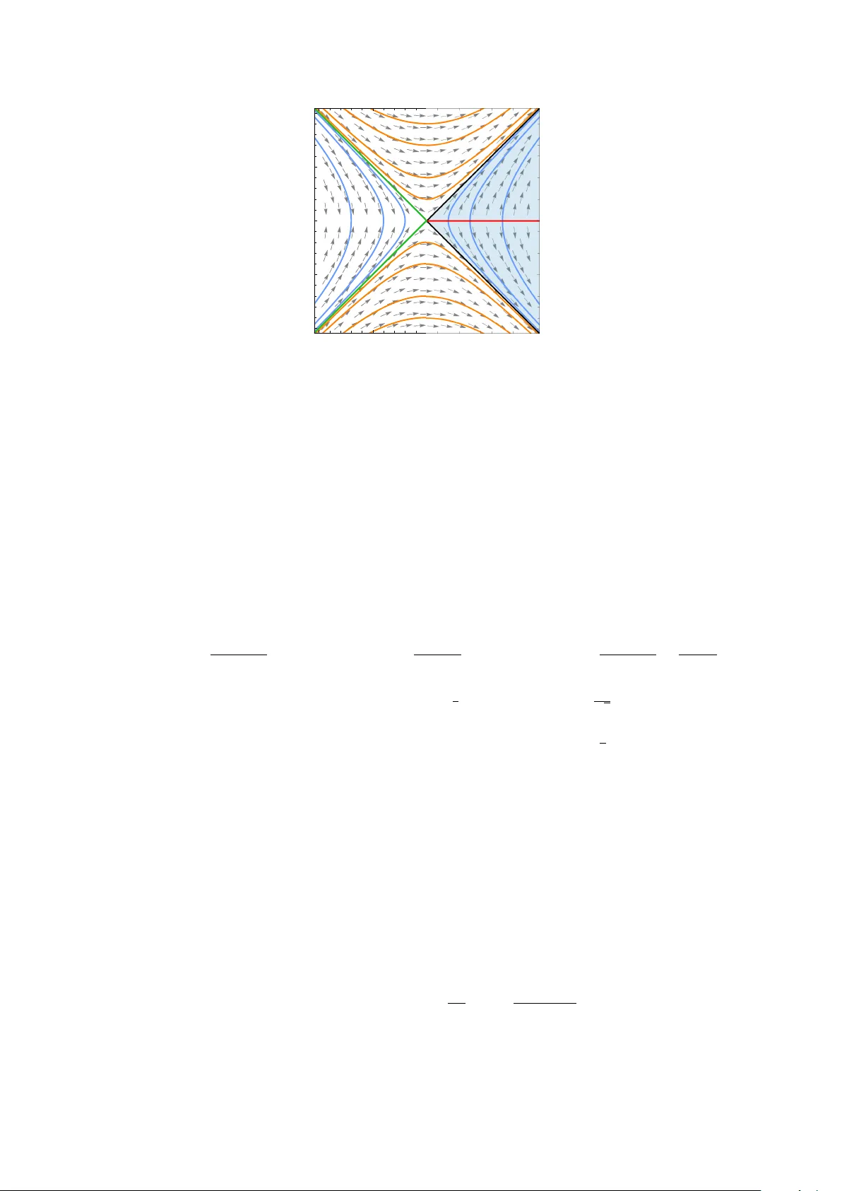
Eﬀectiv e Hamiltonians and Wilson–P olc hinski renormalisation Ric ky Li χ and Benoît Vicedo ¯ χ Departmen t of Mathematics, Universit y of Y ork, Heslington, Y ork YO10 5GH, United Kingdom. Email: χ ricky.li@york.ac.uk , ¯ χ benoit.vicedo@gmail.com F ebruary 2026 Abstract W e dev elop a nov el approac h to the Wilsonian renormalisation of Hamiltonians for 2 - dimensional quantum ﬁeld theories on the cylinder describ ed in the UV by marginally relev an t deformations of conformal ﬁeld theories. T o in tro duce a Wilsonian short-distance cutoﬀ we mak e essential use of free ﬁeld realisations of the full vertex operator algebra in the UV. Our metho d is in trinsically non-p erturbative; we derive a Hamiltonian analogue of Polc hinski’s equation describing the ﬂows of all couplings. As a primary example of our general metho d, we apply it to the marginal anisotropic deformation of the su 2 W ess–Zumino–Witten mo del at level 1 , which is equiv alent to the sine-Gordon mo del on the cylinder. In particular, we repro duce the standard renormali- sation group ﬂo w of the sine-Gordon mo del near the Kosterlitz–Thouless p oin t to second order in the couplings, a result usually deriv ed using Lagrangian/path-in tegral metho ds. Con ten ts 1 In tro duction and ov erview 2 1.1 Approac hes to renormalisation . . . . . . . . . . . . . . . . . . . . . . . . . . . 3 1.1.1 Rigorous p erturbativ e renormalisation . . . . . . . . . . . . . . . . . . . 3 1.1.2 Non-p erturbativ e renormalisation: path-in tegrals . . . . . . . . . . . . . 3 1.1.3 Non-p erturbativ e renormalisation: Hamiltonians . . . . . . . . . . . . . 3 1.2 The Hamiltonian Polc hinski equation . . . . . . . . . . . . . . . . . . . . . . . . 4 1.2.1 F ree ﬁeld realisations and smo oth regularisations . . . . . . . . . . . . . 4 1.2.2 Eﬀectiv e Hamiltonian and Polc hinski’s equation . . . . . . . . . . . . . . 5 1.3 Main example and future directions . . . . . . . . . . . . . . . . . . . . . . . . . 7 2 Bac kground and motiv ation 9 2.1 Curren t algebras . . . . . . . . . . . . . . . . . . . . . . . . . . . . . . . . . . . 9 2.1.1 Chiral and anti-c hiral currents . . . . . . . . . . . . . . . . . . . . . . . 10 2.1.2 F ourier mo de decomp ositions . . . . . . . . . . . . . . . . . . . . . . . . 12 2.1.3 Energy-momen tum tensor . . . . . . . . . . . . . . . . . . . . . . . . . . 13 2.2 F ree ﬁeld realisations . . . . . . . . . . . . . . . . . . . . . . . . . . . . . . . . . 14 1 2.2.1 Chiral and anti-c hiral free b osons . . . . . . . . . . . . . . . . . . . . . . 15 2.2.2 Compactiﬁed b oson and dual b oson . . . . . . . . . . . . . . . . . . . . 18 2.2.3 Changing the compactiﬁcation radius . . . . . . . . . . . . . . . . . . . . 25 3 Renormalisation of Hamiltonians 27 3.1 Regularisation . . . . . . . . . . . . . . . . . . . . . . . . . . . . . . . . . . . . . 27 3.1.1 T runcation vs regularisation . . . . . . . . . . . . . . . . . . . . . . . . . 29 3.1.2 Smo oth regularisations . . . . . . . . . . . . . . . . . . . . . . . . . . . . 32 3.1.3 Asymptotics of harmonic sums . . . . . . . . . . . . . . . . . . . . . . . 36 3.1.4 Regularised vertex op erators . . . . . . . . . . . . . . . . . . . . . . . . 40 3.2 Eﬀectiv e Hamiltonians . . . . . . . . . . . . . . . . . . . . . . . . . . . . . . . . 42 3.2.1 Short/long distance splitting . . . . . . . . . . . . . . . . . . . . . . . . 43 3.2.2 In tegrating out a thin shell . . . . . . . . . . . . . . . . . . . . . . . . . 46 3.2.3 Renormalisation group ﬂow . . . . . . . . . . . . . . . . . . . . . . . . . 54 4 The quan tum sine-Gordon mo del on S 1 59 4.1 The Sine-Gordon Hamiltonian . . . . . . . . . . . . . . . . . . . . . . . . . . . . 59 4.1.1 Anisotropic deformation of the WZW mo del . . . . . . . . . . . . . . . . 59 4.1.2 Rewriting as the sine-Gordon Hamiltonian . . . . . . . . . . . . . . . . . 61 4.2 In tegrating out a thin shell . . . . . . . . . . . . . . . . . . . . . . . . . . . . . 63 4.2.1 δ H ϵ ′ 22 v ariation . . . . . . . . . . . . . . . . . . . . . . . . . . . . . . . . . 65 4.2.2 δ H ϵ ′ 21 and δ H ϵ ′ 12 v ariations . . . . . . . . . . . . . . . . . . . . . . . . . . . 67 4.2.3 δ H ϵ ′ 11 v ariation . . . . . . . . . . . . . . . . . . . . . . . . . . . . . . . . . 70 4.3 Renormalisation group ﬂows . . . . . . . . . . . . . . . . . . . . . . . . . . . . . 75 4.3.1 Irrelev an t coupling contributions . . . . . . . . . . . . . . . . . . . . . . 76 4.3.2 Berezinskii–K osterlitz–Thouless transition . . . . . . . . . . . . . . . . . 77 A Asymptotic expansion of G ( u ; ϵ ) 78 B Asymptotics of a family of double in tegrals 80 B.1 Asymptotics of the double integrals I k . . . . . . . . . . . . . . . . . . . . . . . 80 B.2 Asymptotics of the double integrals J k . . . . . . . . . . . . . . . . . . . . . . . 81 1 In tro duction and o v erview Renormalisation is one of the cornerstones of quan tum ﬁeld theory . The sub ject has ev olved from the p erturbativ e “subtraction of inﬁnities” in F eynman diagram computations in early quan tum electro dynamics to the Wilsonian paradigm [ KW ], whic h formulates quantum ﬁeld theory in terms of scale-dependent eﬀective descriptions. F rom this mo dern p ersp ectiv e, the renormalisation group formalises the relationship betw een eﬀective quan tum ﬁeld theories deﬁned at diﬀerent energy scales (inv erse-length scales), with high-energy degrees of freedom systematically and contin uously integrated out to yield lo w-energy descriptions. 2 1.1 Approac hes to renormalisation 1.1.1 Rigorous p erturbativ e renormalisation The rigorous mathematical underpinning of the p erturbativ e “subtraction of inﬁnities” was the culmination of a substan tial bo dy of work spanning several decades. It b egan with the com binatorial study of nested divergences in F eynman graphs, formalised in the Bogolyub o v– P arasiuk–Hepp–Zimmermann (BPHZ) theorem [ BP , H , Zi ]. This established that lo cal coun- terterms can b e recursiv ely constructed so as to render n -p oin t Green’s functions ﬁnite to all orders in p erturbation theory (see, for instance, [ Coll ]). The BPHZ renormalisation scheme ﬁnds its rigorous justiﬁcation in the causal Epstein–Glaser axiomatic framework [ EG ], in which renormalisation arises from the non-unique extension of time-ordered op erator-v alued distri- butions to coinciden t points rather than from the subtraction of div ergent in tegrals. Finally , Connes and Kreimer sho wed [ CK1 , CK2 ] that the BPHZ recursion is equiv alent to the Birkhoﬀ factorisation of regularised F eynman rules view ed as characters of the Hopf algebra of F eynman graphs [ Kr1 ], thereby recasting p erturbativ e renormalisation as a Riemann–Hilb ert problem. 1.1.2 Non-p erturbativ e renormalisation: path-in tegrals The developmen t of the exact, functional, or non-p erturbativ e renormalisation group in the ph ysics literature ran parallel to these mathematical adv ances in p erturbativ e quan tum ﬁeld theory . Building on Kadanoﬀ ’s coarse-graining intuition [ K ], Wilson cast quantum ﬁeld theory as a ﬂow of eﬀective actions obtained b y successiv ely integrating out high-energy mo des [ KW ]. This physical picture was ﬁrst enco ded in to exact functional diﬀerential equations by W eg- ner and Houghton [ WH ] using a sharp momen tum cutoﬀ, whic h Polc hinski then signiﬁcantly impro ved upon b y w orking instead with a smo oth cutoﬀ regulator [ P ol ]. This ﬂo w equation w as subsequently reformulated b y W etteric h [ W e ] in terms of the so-called eﬀective av erage action. The resulting W etterich equation is mathematically equiv alen t to Polc hinski’s via a functional Legendre transform, but pro vides a formulation in terms of macroscopic observ- ables that is often more suitable for non-p erturbativ e appro ximation schemes and numerical analysis; see e.g. [ BTW , Del , Du+ ] for extensive reviews. It was only relativ ely recently that Costello established a rigorous mathematical foundation for this Wilsonian approac h in the con text of Euclidean quantum ﬁeld theory [ Cos ], see also [ CG2 ], by combining the concept of eﬀectiv e actions with the Batalin–Vilk ovisky formalism. Finally , the incorp oration of these functional ﬂow metho ds into the Lorentzian framew ork of p erturbativ e algebraic quantum ﬁeld theory was recently ac hieved in [ DDPR , DR ], thereby reconciling the Wilsonian in tuition with the rigorous axioms of lo cal cov ariance. 1.1.3 Non-p erturbativ e renormalisation: Hamiltonians Most formulations of Wilsonian renormalisation are ro oted in the path-integral formalism or in p erturbativ e Lagrangian framew orks, where the construction of the S-matrix typically relies on the time-ordering in tuition of the Dyson series. Somewhat surprisingly , comparativ ely less attention has b een dev oted to the Hamilto- nian coun terpart, despite the fact that Wilson’s original intuition [ KW , W ] was inherently based on the diagonalisation of the Hamiltonian matrix in a basis of truncated states. This op erator-theoretic approach w as explicitly formalised by Głazek and Wilson [ GWi1 , GWi2 ] and W egner [ W eg ] through the metho d of contin uous unitary similarity transformations to de- 3 couple high-energy mo des, a metho d known as the ‘Similarity Renormalisation Group’, while related schemes w ere developed in [ MN , GW e , W a , AM1 , AM2 ]. In the T runcated Conformal Space Approac h (TCSA) dev elop ed in [ YZ ], a marginally rel- ev an t p erturbation V of a conformal ﬁeld theory with Hamiltonian H 0 = L 0 + ¯ L 0 is studied n u- merically b y truncating the Hilb ert space of the conformal ﬁeld theory to the ﬁnite-dimensional subspace of states with energy b ounded by some ﬁxed E max . In this setting, Wilsonian renor- malisation tec hniques hav e b een n umerically used to reduce the dep endence of the results on the cutoﬀ E max coming from the truncation, see for instance [ FGPTW , GiW a , R V ]. More recen tly , an extensiv e Hamiltonian renormalisation programme has b een developed b y Thiemann and collab orators, see for instance [ LL T1 , LL T2 , TZ , R T ], which provides a rigorous implemen tation of Kadanoﬀ ’s coarse-graining idea in the Hamiltonian formalism. Sp eciﬁcally , in this approach, op erator v alued distributions are smeared using ﬁnite-dimensional spaces of test functions lab elled b y integer resolution scales M ∈ Z ≥ 1 and the coarse-graining map is deﬁned from a ﬁner graining M ′ to a coarser one M < M ′ . 1.2 The Hamiltonian Polc hinski equation The main goal of this paper is to derive a Hamiltonian analogue of P olchinski’s equation for eﬀectiv e Hamiltonians in the Wilsonian framework. W e formulate our approach for quantum ﬁeld theories on the cylinder S 1 × R , with spatial compactiﬁcation x ∼ x + L , describ ed in the UV b y relev an t or marginally relev an t deformations of 2 -dimensional conformal ﬁeld theories. W e summarise b elo w the con tent of § 3 where this framew ork is dev elop ed. 1.2.1 F ree ﬁeld realisations and smo oth regularisations Standard applications of the Wilsonian renormalisation group t ypically deal with scalar ﬁelds ϕ ( x ) on R d , where the separation of scales is implemented b y a sharp momentum cutoﬀ on the F ourier modes ˆ ϕ ( k ) . W e are in terested in p erturbations of 2 -dimensional conformal ﬁeld theories in the UV, whic h may not intrinsically b e describ ed in terms of free ﬁelds. T o adapt the standard Wilsonian philosophy , our starting p oin t is therefore to make a choice of a free ﬁeld realisation of the underlying full vertex op erator algebra. This is to b e contrasted with Costello’s approach [ Cos ] which employs the BV formalism and homological metho ds to treat general interacting theories without necessarily mapping them to free ﬁelds. Ho wev er, the compact spatial geometry of the cylinder S 1 × R introduces another tec hnical subtlet y: the F ourier mo des of Hamiltonian ﬁelds on S 1 are discrete. In this setting, a standard sharp cutoﬀ on the mo de num b ers n ∈ Z would necessarily b e an in teger, making it imp ossible to deriv e con tinuous renormalisation group ﬂow equations in the form of diﬀeren tial equations with resp ect to the scale. T o circumv ent this, we must esc hew sharp truncations in fa vour of smo oth regularisations . So instead of truncating the algebra of F ourier mo des, we in tro duce a contin uous regulator directly into the canonical comm utation relations of the free ﬁelds, as detailed in § 3.1 . F or concreteness, consider a chiral free b oson χ ( x ) with mo des b n for n ∈ Z satisfying the standard Heisen b erg Lie algebra relations [ b n , b m ] = nδ n + m, 0 . In the regularised theory with short-distance cutoﬀ ϵ > 0 w e replace it b y a smoothly regularised c hiral free b oson χ ϵ ( x ) whose mo des b ϵ n for n ∈ Z satisfy the mo diﬁed relations [ b ϵ n , b ϵ m ] = n η  2 π | n | ϵ L  δ n + m, 0 , (1.1) 4 where the regulator η : R ≥ 0 → R is a ﬁxed but arbitrary smo oth function such that η (0) = 1 and η ( x ) deca ys faster than any p o wer as x → ∞ . This smo oth regularisation cures the ultra violet divergences inherent in the short-distance singularities of pro ducts of c hiral b osons, which typically manifest as divergen t series P ∞ n =1 n s . Indeed, in the regularised theory these are replaced by ﬁnite, alb eit ϵ -dep endent, series of the form P ∞ n =1 n s η  2 π nϵ L  . More imp ortan tly , when the same regularisation is applied also to the an ti-chiral sector, op erators whic h induce deformations aw ay from the conformal ﬁeld theory , giv en by zero-mo des of pro ducts of chiral and anti-c hiral op erators, hav e a well-deﬁned action on the F o c k space of the free ﬁeld realisation. A protot ypical example is the radius-changing op erator R L 0 dx ∂ x χ ( x ) ∂ x ¯ χ ( x ) in the free compactiﬁed b oson conformal ﬁeld theory . 1.2.2 Eﬀectiv e Hamiltonian and Polc hinski’s equation Since the short-distance cutoﬀ ϵ > 0 used in ( 1.1 ) was arbitrary , ph ysical observ ables in the theory should not dep end on it. Indeed, the core philosophy of Wilsonian renormalisation (see, for instance, [ Hol ]) is that there is a notion of ‘separation of scale’ in the sense that the details of the physics at length scales below the one we are concerned ab out should not be relev an t. In particular, physics at length scales longer than the cutoﬀ ϵ > 0 should b e indep enden t of ϵ . T o describ e ho w we implemen t this idea in our setup, we fo cus here again for concreteness on a theory with ﬁeld conten t describ ed b y a chiral and anti-c hiral b oson χ ( x ) and ¯ χ ( x ) . Given an y tw o scales ϵ ′ > ϵ > 0 , w e introduce a ‘shell’ chiral b oson χ ϵ ′ ∖ ϵ ( x ) with mo des b ϵ ′ ∖ ϵ n for ev ery n ∈ Z sub ject to certain commutation relations such that the mo des of χ ϵ ′ ( x ) + χ ϵ ′ ∖ ϵ ( x ) satisfy the same comm utation relations as those of χ ϵ ( x ) giv en in ( 1.1 ); and lik ewise for the an ti-chiral sector. Then the Hamiltonian analogue of the pro cedure of ‘integrating out’ degrees of freedom b et w een the cutoﬀs ϵ and ϵ ′ amoun ts to the problem of constructing an eﬀective Hamiltonian H ϵ ′ eﬀ in the theory with larger cutoﬀ ϵ ′ , i.e. built from the chiral and an ti-chiral ﬁelds χ ϵ ′ ( x ) and ¯ χ ϵ ′ ( x ) , which describ es the same ph ysics as the original Hamiltonian H ϵ in the theory with smaller cutoﬀ ϵ , i.e. built from the chiral and anti-c hiral ﬁelds χ ϵ ( x ) and ¯ χ ϵ ( x ) . Our approac h to deﬁning the eﬀective Hamiltonian H ϵ ′ eﬀ , sp elled out in detail in § 3.2 , is to require that its imaginary-time ev olution o ver an arbitrary but ﬁxed time T matc hes the imaginary-time evolution of the original Hamiltonian H ϵ at the low er cutoﬀ ϵ pro jected do wn to the long-distance subspace, namely e − T H ϵ ′ eﬀ = P l e − T H ϵ P l . (1.2) Here P l denotes the pro jection onto the long-distance subspace, which consists of states where none of the ‘shell mo des’ b ϵ ′ ∖ ϵ n are excited, i.e. the subspace where the shell sector is in its v acuum state. In other w ords, the op erator on the right hand side of ( 1.2 ) describ es the full imaginary-time evolution of all states in the long-distance subspace whic h end up back in this subspace after an imaginary-time T , including all virtual excursions in to the short- distance sector. The eﬀectiv e Hamiltonian H ϵ ′ eﬀ on the left hand side of ( 1.2 ) enco des the same imaginary-time evolution ov er a time T but without ever lea ving the long-distance subspace, incorp orating the eﬀectiv e dynamics of the shell degrees of freedom in the ﬁelds χ ϵ ′ ∖ ϵ ( x ) and ¯ χ ϵ ′ ∖ ϵ ( x ) which hav e b een eliminated or ‘integrated out’. This matc hing of ev olution op erators is similar in spirit to the path-integral formulation of Wilsonian renormalisation in the presence of a high-energy cutoﬀ. There the eﬀectiv e action S Λ ′ eﬀ [ ϕ Λ ′ ] for the low-energy ﬁeld ϕ Λ ′ in the theory with cutoﬀ Λ ′ is deﬁned b y integrating out 5 shell degrees of freedom ϕ Λ ∖ Λ ′ b et w een the cutoﬀs Λ ′ < Λ in the path-integral, namely e − S Λ eﬀ [ ϕ Λ ′ ] = Z D ϕ Λ ∖ Λ ′ e − S Λ [ ϕ Λ ′ + ϕ Λ ∖ Λ ′ ] , (1.3) where S Λ [ ϕ Λ ] denotes the action for the high-energy ﬁeld ϕ Λ = ϕ Λ ′ + ϕ Λ ∖ Λ ′ in the theory with cutoﬀ Λ . Our deﬁnition ( 1.2 ) of the eﬀective Hamiltonian H ϵ ′ eﬀ can b e viewed as a Hamiltonian analogue of this standard deﬁnition ( 1.3 ) of the eﬀective action. Indeed, one of the main results of the pap er, see § 3.2.3 , is a Hamiltonian analogue of P olchinski’s equation [ Pol ] deriv ed using ( 1.2 ) in the case when the length scale cutoﬀ v aries inﬁnitesimally so that ϵ ′ = ϵ + δ ϵ for small δ ϵ . By working to leading order in δ ϵ we derive the b eta function for all the couplings. Our deﬁnition of the eﬀective Hamiltonian in ( 1.2 ) diﬀers conceptually from the one used in the Similarity Renormalisation Group [ GWi1 , GWi2 , W eg , MN , GW e , W a , AM1 , AM2 ]. The k ey idea b ehind this approach is to seek a unitary similarity transformation of the Hamiltonian H Λ in the theory with cutoﬀ Λ which decouples the shell degrees of freedom b et ween the cutoﬀs Λ ′ < Λ from the lo w-energy ones b elo w the cutoﬀ Λ ′ . In other words, one is after a unitary op erator U Λ , Λ ′ suc h that the transformed Hamiltonian U Λ , Λ ′ H Λ U † Λ , Λ ′ is blo c k-diagonal with resp ect to the lo w- and high-energy subspaces, so that it sends, in particular, the low-energy subspace to itself. The eﬀective Hamiltonian at the cutoﬀ Λ ′ is then giv en simply by restricting this transformed Hamiltonian to the low-energy subspace, i.e. H Λ ′ eﬀ = P l U Λ , Λ ′ H Λ U † Λ , Λ ′ P l (1.4) where P l is the pro jection onto the lo w-energy subspace. In practice, how ever, the Hamiltonian H Λ can only b e blo c k-diagonalised p erturbativ ely to the ﬁrst few orders in b oth the couplings and the ratio of energy scales Λ ′ / Λ , see for instance [ AM2 ] for a nice application of these ideas to the 4 -dimensional φ 4 theory . In this approach, the virtual excursions in to the shell sector are captured b y the unitary transformation which can eﬀectively b e seen as mapping the free v acuum state of the shell sector in the regularised theory to the interacting one. There are also similarities b et ween our deﬁnition ( 1.2 ) and the construction of the eﬀectiv e Hamiltonian in the recen tly prop osed Hamiltonian T runcation Eﬀective Theory [ CFHL , DFH ]. In the metho d of Hamiltonian T runcation ﬁrst in tro duced in [ BF ], or the T runcated Conformal Space Approac h of [ YZ ], the truncated Hamiltonian is P l ( H 0 + V )P l , where P l here denotes the pro jection on to the ﬁnite-dimensional subspace of states with total energy less than some cutoﬀ E max , whic h can b e diagonalised n umerically . Hamiltonian T runcation Eﬀectiv e Theory [ CFHL , DFH ], see also the v ery recen t pap er [ MRP ], oﬀers a systematic wa y of improving on the naive truncation P l ( H 0 + V )P l of the Hamiltonian b y using metho ds from eﬀective ﬁeld theory to construct an eﬀectiv e Hamiltonian whic h takes into account the eﬀects from states ab o v e the cutoﬀ E max . How ever, rather than use a similarit y transformation as in ( 1.4 ), the eﬀectiv e Hamiltonian is obtained by matching its transition amplitudes b et ween low-energy states to the transition amplitudes of the full Hamiltonian b et w een the same states. The approaches of the Similarit y Renormalisation Group and of Hamiltonian T runcation Eﬀectiv e Theory describ ed ab ov e are b oth inﬂuenced by well-kno wn methods to calculate eﬀectiv e Hamiltonians, suc h as Rayleigh–Sc hrö dinger p erturbation theory or Schrieﬀer–W olﬀ transformations [ SW , BDL ]. Y et it is imp ortan t to observ e that these metho ds rely on a sharp separation of energy scales in the sp ectrum of the unp erturb ed theory since they t ypically in volv e denominators ( E h − E l ) − 1 with diﬀerences b et ween energy eigenv alues E h and E l in 6 the high-energy and low-energy sectors. But in a smo oth regularisation scheme lik e the one w e are using ( 1.1 ), following Polc hinski’s original approac h to Wilsonian renormalisation using smo oth high-energy cutoﬀs [ Pol ], the ‘shell’ mo des to b e in tegrated out in the construction of the eﬀectiv e Hamiltonian inevitably include a tail with arbitrarily lo w energies, causing these energy denominators to diverge. Our deﬁnition ( 1.2 ) of the eﬀective Hamiltonian, which closely mimics the path-in tegral deﬁnition of the eﬀectiv e action used in [ Pol ], does not rely on the existence of an energy gap b et ween short- and long-distance degrees of freedom. Finally , let us note that the use of smo oth regularisation in p erturbativ e renormalisation has independently b een explored in the recen t w orks [ PS1 , PS2 ]. Their motiv ation for using smo oth regularisations was also inspired by [ T ao ], see § 3.1 , and so it w ould b e interesting to understand if the framew ork developed in these pap ers is related to ours. 1.3 Main example and future directions The main example to whic h we apply the metho ds developed in § 3 , brieﬂy outlined ab o ve in § 1.2 , is the sine-Gordon mo del. W e summarise b elo w the con tent of § 4 where this example is studied in detail. The quan tum sine-Gordon mo del is a tremendously w ell studied quan tum ﬁeld theory in 2 dimensions, with a v ast literature initiated by Coleman’s seminal work [ Col ] on its equiv a- lence to the massiv e Thirring mo del. This theory is sim ultaneously ric h in non-p erturbativ e phenomena, in particular through its strong/weak coupling duality with the massiv e Thirring mo del, see e.g. [ Ma ], yet suﬃciently simple to be tractable, owing in part to its in tegrability [ KN , ZZ , STF , Za , NT ] (see also [ T o ] for a recent review). As suc h, it pro vides an ideal test- ing ground for exploring new and existing frameworks in 2 -dimensional quantum ﬁeld theory , whic h explains wh y the literature on the sine-Gordon mo del contin ues to rapidly expand even to this day . In particular, recen t progress w as made on describing the sine-Gordon mo del from the p ersp ectiv e of p erturbativ e algebraic quan tum ﬁeld theory [ BR , Zan ]. A remark able feature of the quantum sine-Gordon mo del is that its renormalisation group ﬂo w exhibits the famous Berezinskii–Kosterlitz–Thouless (BKT) transition [ B1 , B2 , KT ]. This phase transition, c haracterised by a separatrix dividing the massless and massive phases, has b een derived in many diﬀerent formalisms. F or instance, it w as originally derived using p er- turbativ e Wilsonian renormalisation tec hniques on the XY-mo del [ Ko ], whic h lies in the same univ ersality class as the sine-Gordon mo del, and later using standard ﬁeld-theoretic countert- erm renormalization around the Kosterlitz–Thouless p oin t [ AGG , BH ], using string theoretic metho ds [ Lo ], using Polc hinski’s equation [ OaSa ] or using conformal p erturbation theory , see e.g. [ F ra , §4.6]. W e refer also to [ F rS , MKP ] for rigorous deriv ations and to [ DH1 , DH2 , DH3 ] where rigorous Euclidean path-integral methods are used, relating to the framew ork of con- struction quantum ﬁeld theory [ GJ ]. While the BKT transition is seen already at second order in the couplings around the K osterlitz–Thouless p oin t within these p erturbativ e frameworks, the renormalisation group ﬂo w of the sine-Gordon mo del has also b een extensively studied non- p erturbativ ely using the functional renormalisation group, namely via the W etterich equation, see for instance [ NNPS1 , NNPS2 , DD ] and also [ HJMSN ] for a recen t comparison b et ween the non-p erturbativ e and p erturbativ e analyses. Imp ortan tly for us, the sine-Gordon mo del on the cylinder can b e describ ed as a marginally relev an t p erturbation of a 2-dimensional conformal ﬁeld theory in the UV, namely the free b oson compactiﬁed at the self-dual radius. Explicitly , the sine-Gordon mo del is equiv alen t to 7 an anisotropic deformation of the su 2 WZW mo del at level 1 [ BL1 , §3g], with Hamiltonian H sG = 2 π L ( L 0 + ¯ L 0 ) + g 1 4 π Z L 0 d x  J + ( x ) ¯ J − ( x ) + J − ( x ) ¯ J + ( x )  + g 2 8 π Z L 0 d x J 3 ( x ) ¯ J 3 ( x ) . (1.5) The ﬁrst term on the right hand side is the Hamiltonian of the su 2 WZW mo del and the tw o J ¯ J -deformations are written in terms of the chiral and anti-c hiral su 2 -curren ts of the WZW mo del. The relationship with the sine-Gordon mo del, whic h is describ ed by a single b oson ﬁeld Φ( x ) and its conjugate momentum Π( x ) , is seen directly by recalling that the chiral and an ti- c hiral su 2 -curren ts at level 1 admit a free ﬁeld realisation in terms of chiral and an ti-c hiral free b osons χ ( x ) and ¯ χ ( x ) , resp ectiv ely; see § 2.2 and § 4.1 for details. Under this free ﬁeld realisation the kinetic term of the sine-Gordon Hamiltonian arises as the sum of the ﬁrst and last terms in ( 1.5 ), with the chiral decomp ositions Φ( x ) = ϕ ( x ) + ¯ ϕ ( x ) and Π( x ) = ∂ x ϕ ( x ) − ∂ x ¯ ϕ ( x ) related to the c hiral and an ti-chiral ﬁelds χ ( x ) and ¯ χ ( x ) by a Bogolyub o v transformation; see § 2.2.3 and § 4.1.2 for details. In particular, the last term in ( 1.5 ) is the marginal p erturbation inducing a radius c hange in the compactiﬁed free b oson from the self-dual radius to a generic radius R = 2 /β determined b y g 2 . The second term in ( 1.5 ) then b ecomes prop ortional to the standard cosine p oten tial R L 0 d x ⦂ cos( β Φ( x )) ⦂ β whic h is relev an t for β 2 < 8 π ; see § 4.1.2 . As a non-trivial chec k of our approach to Wilsonian renormalisation in the Hamiltonian formalism using a smo oth regularisation à la Polc hinski, outlined in § 1.2 , the main goal of § 4 is to rederive the renormalisation group ﬂow equations to second order of the marginal couplings g 1 and g 2 in ( 1.5 ), with resp ect to the contin uous short-distance cutoﬀ scale ϵ > 0 . With our normalisation conv entions we recov er the well-kno wn renormalisation group ﬂo w ϵ∂ ϵ g 1 = g 1 g 2 , ϵ∂ ϵ g 2 = g 2 1 (1.6) whic h exhibits the BKT transition; see Figure 1 in the main text. The renormalisation group ﬂo w ( 1.6 ) is universal, i.e. scheme indep enden t, and w as giv en in [ Za ]. In fact, the ﬂow derived in [ Za ] is an all-lo op exact expression in a particular renormalisation sc heme, obtained using the Poincaré–Dulac theorem to ﬁx the renormalisation sc heme ambiguit y of the subleading co eﬃcien ts. Note that a diﬀeren t all-lo op extension of the universal leading-order ﬂo w ( 1.6 ) w as also given in [ BL2 , §I I I]. The latter is based on a conjectured exact expression for the b eta function of curren t-current deformations of 2 -dimensional conformal ﬁeld theories with Kac–Mo ody current-algebra symmetry [ GLM ], obtained using W ard iden tity considerations. Ho wev er, a subsequen t 4 -lo op computation of this renormalisation group ﬂow using conformal p erturbation theory in [ L W ] w as found to b e incompatible with the ﬂo w of [ BL2 , §II I] in an arbitrary renormalisation sc heme. It w ould b e interesting to push the computations in the presen t Hamiltonian framew ork to higher order in p erturbation theory to c heck these all-lo op exact extensions of the universal renormalisation group ﬂow ( 1.6 ). Finally , it would b e in teresting to apply the Hamiltonian framework developed in this pap er to other 2 -dimensional quan tum ﬁeld theories on the cylinder S 1 × R , whic h can b e describ ed b y marginally relev ant deformations of conformal ﬁeld theories in the UV. F or concreteness we ha ve fo cused on the su 2 WZW mo del at level 1 b ecause the asso ciated (anti-)c hiral su 2 -curren t algebra admits a simple realisation in terms of a single free (anti-)c hiral b oson. How ever, the metho d is exp ected to b e applicable muc h more generally to any quan tum ﬁeld theory whose conformal ﬁeld theory in the UV can b e realised in terms of arbitrarily many free ﬁelds suc h as (anti-)c hiral b osons, fermions, β γ -systems or bc -systems. 8 An obvious ﬁrst step would b e to explore the Wilsonian renormalisation ﬂow of the massive Thirring mo del, recently derived using functional renormalisation group metho ds in [ NKOP ], b y realising the (anti-)c hiral su 2 -curren t algebra at level 1 in terms of free (anti-)c hiral fermions instead of b osons, see [ F re ]. Another natural next step is to apply our approach to aﬃne T o da ﬁeld theories asso ciated with higher rank Lie algebras g , for which the renormalisation group equations hav e been derived using standard p erturbativ e metho ds and whic h are kno wn to exhibit generalised BKT transitions [ GLPZ , GP , BL1 ]. Notably , the construction presented here for su 2 should admit a direct generalisation to higher rank in the case of simply-laced g where the asso ciated un twisted aﬃne Kac–Mo ody algebra also has a basic represen tation in terms of rk g b osons via the F renkel–Kac construction; see [ FK ] and [ Kac2 , §5.6]. A particularly in teresting direction for future research would b e the application of these metho ds to integrable σ -models suc h as the Klimčík mo del [ Kli ]. Indeed, the study of its UV limit in [ KL T ] serv ed as one of the primary motiv ations for the presen t work, whic h seeks to provide a systematic framew ork for constructing 2 -dimensional quantum ﬁeld theories that are describ ed in the UV as p erturbations of conformal ﬁeld theories with free ﬁeld realisations. A ckno wledgemen ts W e w ould like to thank Edoardo D’Angelo, Ben Hoare, Sylv ain Lacroix, Nat Levine, Enrique Moreno, Sandor Nagy , Istv an Nandori, Stefano Negro, Antonio Padilla, Rob ert Smith and Alessandro T orrielli for useful discussions and corresp ondences in relation to v arious asp ects of this work. The authors gratefully ackno wledge the supp ort of the Leverh ulme T rust through a Lev erhulme Research Pro ject Grant (RPG-2021-154). B.V. also gratefully ackno wledges the supp ort of the Engineering and Physical Sciences Research Council (UKRI1723). 2 Bac kground and motiv ation W e are interested in studying the renormalisation group ﬂows of 2 -dimensional quantum ﬁeld theories whose b eha viour in the ultraviolet is describ ed by marginally relev an t p erturbations of 2 -dimensional conformal ﬁeld theories. F or ease of presentation, to motiv ate our approach we fo cus on a particular class of 2 -dimensional conformal ﬁeld theories, the W ess–Zumino–Witten (WZW) mo dels, whic h exhibit left and right aﬃne Kac–Mo ody algebra symmetries generated b y chiral and an ti-chiral curren ts. In this setting, the marginally relev ant op erator inducing the renormalisation group ﬂow is a bilinear com bination of these chiral and anti-c hiral currents. Throughout the rest of the pap er w e shall, in fact, further sp ecialise to a particular instance of this general setting which corresp onds to the sine-Gordon mo del, to b e discussed in § 4 . In this section we will therefore present the bac kground relev ant for this particular case, but we exp ect the techniques outlined in the pap er to b e applicable muc h more generally . 2.1 Curren t algebras W e recall the deﬁnition of the un twisted aﬃne Kac–Mo ody algebra in terms of generators and relations in § 2.1.1 . T wo comm uting copies of this algebra, enco ded in the chiral and an ti-chiral curren ts, generate the full aﬃne vertex algebra which underpins the conformal structure of the W ess–Zumino–Witten mo del [ DMS , §15]. Since w e will b e primarily in terested in the example of the Lie algebra sl 2 , w e discuss the sp eciﬁcs of this case alongside the general story . In § 2.1.2 w e describe the usual change of v ariable from the plane to the cylinder [ DMS ], giving rise to 9 F ourier mo de decomp ositions of the chiral and anti-c hiral currents on S 1 . Imp ortan tly , there is a subtle diﬀerence in sign b et ween the currents which leads to a whole class of lo cal op erators, coupling the tw o chiralities together, whose careful treatmen t will require renormalisation. In § 2.1.3 we recall the deﬁnition of the chiral and an ti-c hiral Virasoro generators in terms of the curren ts and express the Hamiltonian of the WZW mo del in terms of the zero-mo des of the stress-energy tensor. 2.1.1 Chiral and anti-c hiral curren ts Aﬃne Kac–Mo o dy algebras can b e obtained as central extensions of lo op algebras asso ciated with any ﬁnite-dimensional semisimple complex Lie algebra g . Giv en an arbitrary basis J a for a = 1 , . . . , dim g of the Lie algebra g , w e let f ab c denote the asso ciated structure constants, so that [ J a , J b ] = P c f ab c J c . When the reality conditions imp osed are suc h that ( J a ) † = J a , it is customary to include an extra factor of i on the righ t hand side so that f ab c is real; see e.g. [ DMS , (13.2)]. W e will b e interested in diﬀerent realit y conditions so w e do not follow this conv ention. Let κ : g × g → C b e the normalised Killing form on g deﬁned for any x , y ∈ g by κ ( x , y ) : = 1 2 h ∨ tr  ad ( x ) ad ( y )  , where h ∨ is the dual Co xeter num b er of g , and denote its comp onen ts by κ ab = κ ( J a , J b ) . The comp onen ts deﬁne an inv ertible matrix, since κ is non-degenerate, and we denote the comp onents of its inv erse b y κ ab . In the case g = sl 2 of interest in this pap er, we ﬁx a standard basis of J 3 , J + and J − with relations [ J + , J − ] = J 3 , [ J 3 , J ± ] = ± 2 J ± . (2.1) The dual Coxeter num b er of sl 2 is h ∨ = 2 so that κ ( J 3 , J 3 ) = 2 and κ ( J + , J − ) = 1 . The unt wisted aﬃne Kac–Mo ody algebra asso ciated with g is an inﬁnite dimensional Lie algebra, with generators J a n for a = 1 , . . . , dim g and n ∈ Z , and Lie brac ket given by [ J a n , J b m ] = X c f ab c J c n + m + k κ ab nδ n + m, 0 , (2.2a) where k ∈ C is called the level. In the c hosen normalisation of the Killing form, the so-called critic al lev el is − h ∨ and we shall henceforth assume that k  = − h ∨ . Strictly sp eaking, the lev el k in the abov e algebra ( 2.2a ) should b e replaced by a central element 1 . Ho w ever, when one is only in terested in considering representations of the unt wisted aﬃne Kac–Mo ody algebra b g on which this central elemen t 1 acts as m ultiplication by the num b er k , it is standard to w ork directly with the Lie algebra relations ( 2.2a ) and refer to this as the unt wisted aﬃne Kac-Mo ody algebra b g at level k , often denoted in the literature simply by b g k . W e introduce a second copy of the unt wisted aﬃne Kac–Mo ody algebra whose generators w e denote by ¯ J a n for a = 1 , . . . , dim g and n ∈ Z , satisfying the same Lie algebra relations as in ( 2.2a ), namely [ ¯ J a n , ¯ J b m ] = X c f ab c ¯ J c n + m + k κ ab nδ n + m, 0 . (2.2b) In principle the level k here could b e diﬀerent from the one app earing in ( 2.2a ), but in the example we shall consider b oth levels coincide so we shall only consider this case. T o distinguish this second cop y of the un twisted aﬃne Kac–Mo o dy algebra from b g k deﬁned ab o ve, we shall denote it as b ¯ g k . W e further take these tw o aﬃne Kac–Mo o dy algebras to comm ute, i.e. w e require [ J a n , ¯ J b m ] = 0 , which amounts to working with the direct sum Lie algebra b g k ⊕ b ¯ g k . The inﬁnitely many generators of these tw o aﬃne Kac–Mo ody algebras can b e conv eniently 10 organised into the chiral and an ti-chiral currents as follo ws. T o each basis element J a (or more generally to any elemen t of g ) we can asso ciate a pair of holomorphic and an ti-holomorphic curren ts in a complex v ariable z deﬁned as J a [ z ] : = X n ∈ Z J a n z − n − 1 , ¯ J a [ ¯ z ] : = X n ∈ Z ¯ J a n ¯ z − n − 1 . (2.3) W e use square brac ket notation for the argumen ts z and ¯ z since we reserv e the more standard brac ket notation for the F ourier mo de decomp osition of the same curren ts, see § 2.1.2 b elo w. It is imp ortant to stress here that while ¯ z denotes the complex conjugate of z , the mo des ¯ J a n and J a n are indep enden t, and in particular they are not related b y hermitian conjugation. Instead, hermitian conjugation is deﬁned using a c hoice of anti-linear inv olution τ : g → g on the Lie algebra g , b y letting X † n : = − ( τ X ) − n and ¯ X † n : = − ( τ X ) − n for every X ∈ g and n ∈ Z . Note that the ov erall min us sign in these deﬁnitions is to ensure that ( · ) † deﬁnes an anti-linear anti -inv olution on the F ourier mo des. When g = sl 2 w e tak e τ : sl 2 → sl 2 to b e the anti-linear in volution deﬁning the compact real form su 2 of sl 2 , given by τ J 3 = − J 3 and τ J ± = − J ∓ . W e then hav e ( J 3 n ) † = J 3 − n , ( J ± n ) † = J ∓ − n , ( ¯ J 3 n ) † = ¯ J 3 − n , ( ¯ J ± n ) † = ¯ J ∓ − n . (2.4) In terms of the currents ( 2.3 ), the pair of un twisted aﬃne Kac–Mo ody algebra relations ( 2.2 ) are then equiv alen tly enco ded in the singular part of the op erator pro duct expansions J a [ z ] J b [ w ] ∼ k κ ab ( z − w ) 2 + X c f ab c J c [ w ] z − w , (2.5a) ¯ J a [ ¯ z ] ¯ J b [ ¯ w ] ∼ k κ ab ( ¯ z − ¯ w ) 2 + X c f ab c ¯ J c [ ¯ w ] ¯ z − ¯ w . (2.5b) W e also ha ve the regular op erator pro duct expansion J a [ z ] ¯ J b [ ¯ w ] ∼ 0 whic h enco des the fact that the tw o copies of the aﬃne Kac–Mo ody algebra m utually commute. More general comp osite op erators O [ z , ¯ z ] , whic h may depend on b oth z and ¯ z , can then b e constructed as ﬁnite linear com binations of normal ordered pro ducts of deriv ativ es of the c hiral and an ti-chiral currents ( 2.3 ), namely : 1 m 1 ! ∂ m 1 z J a 1 [ z ] . . . 1 m r ! ∂ m r z J a r [ z ]: : 1 n 1 ! ∂ n 1 ¯ z ¯ J b 1 [ ¯ z ] . . . 1 n s ! ∂ n s ¯ z ¯ J b s [ ¯ z ]: (2.6) with m 1 , . . . , m r , n 1 , . . . , n s ∈ Z ≥ 0 and a 1 , . . . , a r , b 1 , . . . , b s ∈ { 1 , . . . , dim g } for any r, s ∈ Z ≥ 0 . Under the state-ﬁeld corresp ondence, such comp osite op erators in the 2 -dimensional conformal ﬁeld theory corresp ond to particular states in the full aﬃne vertex algebra F k ( g ) . The latter is deﬁned as the mo dule ov er b g k ⊕ b ¯ g k induced from the trivial representation of the p ositiv e part of the Kac–Mo o dy algebra, namely the 1 -dimensional vector space C | 0 ⟩ spanned by the v acuum state | 0 ⟩ with deﬁning prop erties J a n | 0 ⟩ = 0 and ¯ J a n | 0 ⟩ = 0 for all n ≥ 0 and a = 1 , . . . , dim g . Sp eciﬁcally , the state-ﬁeld corresp ondence asso ciates the op erator ( 2.6 ) to the state J a 1 − m 1 − 1 . . . J a r − m r − 1 ¯ J b 1 − n 1 − 1 . . . ¯ J b s − n s − 1 | 0 ⟩ ∈ F k ( g ) . (2.7) W e refer for instance to [ V ] for a detailed description of the full aﬃne vertex algebra F k ( g ) . 11 2.1.2 F ourier mo de decomp ositions W e are in terested in 2 -dimensional ﬁeld theories on the cylinder S 1 × R , where S 1 represen ts the compact spatial direction and R is the time direction. In the Hamiltonian formalism, such a theory is describ ed b y a collection of ﬁelds on a constan t-time Cauch y surface, i.e. a copy of S 1 , which therefore admit F ourier mo de decomp ositions. In the context of a 2 -dimensional conformal ﬁeld theory , this set-up can b e obtained by means of the so-called radial quantisation using a co ordinate transformation from the plane to the cylinder [ DMS , §6.1]. Curren ts on the cylinder. Explicitly , let x ∈ [0 , L ] b e a co ordinate along the circle S 1 where the length scale L ∈ R > 0 represen ts the circumference of the cylinder, and let t ∈ R b e the time co ordinate along the vertical direction on the cylinder. By introducing the complex co ordinate u = x + it on the cylinder, with the p eriodic identiﬁcation u ∼ u + L , we can map the cylinder to the plane using the conformal transformation u 7→ z = e 2 π iu/L . Under the in verse transformation, the chiral and anti-c hiral curren ts ( 2.3 ) then get mapp ed to J a ( u ) = 2 π L z J a [ z ] = 2 π L X n ∈ Z J a n e − 2 π inu/L , (2.8a) ¯ J a ( ¯ u ) = 2 π L ¯ z ¯ J a [ ¯ z ] = 2 π L X n ∈ Z ¯ J a n e 2 π in ¯ u/L , (2.8b) see, e.g., [ V , §4.1]. In the latter, the co ordinate transformation z = e iu 7→ iu is considered but using instead the present co ordinate transformation z = e 2 π iu/L 7→ iu leads to the additional factors of 2 π L . Note, in particular, that ( 2.8 ) are really the expressions for the sl 2 -curren ts in the co ordinate iu , rather than u . On the left hand sides of ( 2.8 ) we introduced the brack et notation for the argumen ts u and ¯ u of the currents on the cylinder, b y contrast with the square brac ket notation used in ( 2.3 ) for the currents on the z -plane. These are sometimes denoted instead as J a cyl. ( u ) and J a pl. ( z ) , resp ectively , and similarly for the anti-c hiral curren ts, see e.g. [ DMS ], but since we will only b e in terested in the cylinder we omit the subscript ‘cyl.’ and instead reserve the brack et notation for the argumen ts of a current on the cylinder. Restricting ( 2.8 ) to the constant time slice u = x ∈ [0 , L ] leads to the desired F ourier mo de decomp ositions J a ( x ) = 2 π L X n ∈ Z J a n e − 2 π inx/L , ¯ J a ( x ) = 2 π L X n ∈ Z ¯ J a n e 2 π inx/L . (2.9) It follo ws using ( 2.4 ) that the currents ( 2.8 ) in the u co ordinate on the cylinder satisfy the simple reality conditions J 3 ( u ) † = J 3 ( ¯ u ) , J ± ( u ) † = J ∓ ( ¯ u ) , ¯ J 3 ( u ) † = ¯ J 3 ( ¯ u ) , ¯ J ± ( u ) † = ¯ J ∓ ( ¯ u ) . (2.10) Lo cal op erators. W e pause here to make a trivial but crucial observ ation ab out the F ourier mo de expansions ( 2.9 ). Notice that the chiral mo des J a n in the expansion of the current J a ( x ) come multiplied by the exp onential e − 2 π inx/L while the anti-c hiral mo des ¯ J a n in the expansion of the current ¯ J a ( x ) come instead multiplied by the inv erse exp onential e 2 π inx/L . This prop ert y stems from the fact that the c hiral and an ti-chiral currents deﬁned in ( 2.3 ) w ere respectively holomorphic and anti-holomorphic in the v ariable z = e 2 π iu/L . 12 And although trivial, this observ ation has imp ortan t implications on which kind of lo cal op erators, i.e. integrals o ver x ∈ S 1 of comp osite op erators of the form ( 2.6 ), are well deﬁned. Indeed, integrals of purely c hiral (or an ti-c hiral) comp osite op erators lead to inﬁnite sums of normal ordered monomials of the form : J a 1 n 1 . . . J a r n r : with n 1 + . . . + n r = 0 . F or instance, when g = sl 2 w e may consider the lo cal op erator 1 2 π Z L 0 d x : J 3 ( x ) J 3 ( x ): = 2 π L X n> 0 J 3 − n J 3 n . (2.11) F rom suc h a normal ordered inﬁnite sum, only ﬁnitely man y terms can act non-trivially on an y given state in a smo oth represen tation of the chiral aﬃne Kac–Mo o dy algebra ( 2.2a ). In stark contrast, the integrals of comp osite op erators ( 2.6 ) comprising b oth chiral and an ti-chiral pieces lead to inﬁnite sums of pro ducts of chiral creation op erators ( J a n with n < 0 ) with anti-c hiral creation op erators ( ¯ J a n with n < 0 ). F or instance, when g = sl 2 an example of a lo cal op erator we will b e in terested in is 1 2 π Z L 0 d x J 3 ( x ) ¯ J 3 ( x ) = 2 π L X n ∈ Z J 3 n ¯ J 3 n . (2.12) The construction of b g k ⊕ b ¯ g k -represen tations on whic h such lo cal op erators hav e a well-deﬁned action requires some care. W e will come bac k to this issue in § 3 b elo w after describing the kind of representation of interest for the sine-Gordon mo del in § 2.2 . 2.1.3 Energy-momen tum tensor T wo imp ortan t comp osite op erators are the holomorphic and anti-holomorphic comp onents of the energy-momentum tensor, whic h generate commuting chiral and anti-c hiral copies of the Virasoro algebra, given by the Suga wara construction T [ z ] : = 1 2( k + h ∨ ) X a,b κ ab : J a [ z ] J b [ z ]: , (2.13a) ¯ T [ ¯ z ] : = 1 2( k + h ∨ ) X a,b κ ab : ¯ J a [ ¯ z ] ¯ J b [ ¯ z ]: . (2.13b) These op erators corresp ond, under the state-ﬁeld corresp ondence of F k ( g ) , to the chiral state Ω : = 1 2 ( k + h ∨ ) − 1 P a,b κ ab J a − 1 J b − 1 | 0 ⟩ and anti-c hiral state ¯ Ω : = 1 2 ( k + h ∨ ) − 1 P a,b κ ab ¯ J a − 1 ¯ J b − 1 | 0 ⟩ , resp ectiv ely . They expand as T [ z ] = P n ∈ Z L n z − n − 2 and ¯ T [ ¯ z ] = P n ∈ Z ¯ L n ¯ z − n − 2 where the c hiral and an ti-chiral Virasoro mo des L n and ¯ L n are given explicitly by L n : = 1 2( k + h ∨ ) X m ∈ Z X a,b κ ab : J a m J b n − m : , (2.14a) ¯ L n : = 1 2( k + h ∨ ) X m ∈ Z X a,b κ ab : ¯ J a m ¯ J b n − m : . (2.14b) These generate tw o commuting copies of the Virasoro algebra with central c harge c = k dim g k + h ∨ . It is w ell know n, see for instance [ DMS , (5.138)] or also [ V , §4.1.2], that under the in verse of the conformal transformation u 7→ z = e 2 π iu/L , the holomorphic and an ti-holomorphic 13 comp onen ts of the energy-momen tum tensor ( 2.13 ) get mapp ed to T ( u ) =  2 π L  2  z 2 T [ z ] − c 24  , ¯ T ( ¯ u ) =  2 π L  2  ¯ z 2 ¯ T [ ¯ z ] − c 24  . (2.15) W e note here the usual shifts b y the constant − c 24 whic h originate from the Sc hw arzian deriv a- tiv e terms in the transformation prop erties of the (anti-)holomorphic comp onen ts of the energy momen tum tensor under conformal transformations [ DMS , §5.4.1]. The Hamiltonian of the WZW mo del on the circle is given in terms of ( 2.15 ) as H 0 : = 1 2 π Z L 0 d x T ( x ) + 1 2 π Z L 0 d x ¯ T ( x ) = 2 π L  L 0 + ¯ L 0 − c 12  . (2.16) 2.2 F ree ﬁeld realisations In view of studying the renormalisation group ﬂow of the WZW mo del p erturbed by marginally relev an t op erators using a Wilsonian-type approach, we ﬁrst need to introduce a Wilsonian cutoﬀ in the WZW mo del. Naturally , it is tempting to regularise the theory b y truncating the (an ti-)chiral Kac–Mo o dy currents at some energy cutoﬀ Λ ∈ Z > 0 , keeping only those F ourier mo des J a n and ¯ J a n whose mo de num b er n satisfy the b ound | n | ≤ Λ . Sp eciﬁcally , this truncation is obtained by quotien ting the direct sum of c hiral and anti-c hiral Kac–Mo ody algebras with deﬁning relations ( 2.2 ) by the ideal ⟨ J a n , ¯ J a n ⟩ | n | > Λ , generated by the basis elemen ts w e w ant to discard. How ev er, we see from the ﬁrst term on the right hand side of ( 2.2 ) that this ideal is in fact equal to the whole algebra. W e will later in tro duce smo oth regularisation in § 3.1.2 for whic h the same problem p ersists. If the underlying Lie algebra g were abelian, how ev er, then only the second term on the righ t hand side of the relation ( 2.2 ) would b e present, i.e. the central extension term, and there w ould be no suc h problem. In this ab elian setting, the unt wisted aﬃne Kac–Mo o dy algebras ( 2.2a ) and ( 2.2b ) corresp ond to c hiral and anti-c hiral Heisen b erg Lie algebras, resp ectiv ely , and describ e the algebras of F ourier mo des of deriv atives of chiral and anti-c hiral fr e e b osons; see § 2.2.1 b elo w. The adjectiv e ‘free’ here refers to the fact that the Lie brac ket of an y t wo mo des is central (we ha ve not yet sp eciﬁed any Hamiltonian). Another imp ortan t example of free b osonic ﬁelds is giv en by the β γ -system, i.e. an inﬁnite-dimensional W eyl algebra. As we will explain shortly in § 3.1 , the algebras of F ourier mo des of fr e e b osonic ﬁelds are easily regularised. In order to regularise the pair of aﬃne Kac–Moo dy algebras ( 2.2 ) w e shall exploit the fact that these alwa ys admit free ﬁeld realisations, suc h as free fermion represen tations or the W akimoto realisation which utilises a collection of b oth free chiral b osons and β γ -systems. F or simplicit y , in this pap er w e shall fo cus on the simplest type of free ﬁeld realisation of the un twisted aﬃne Kac–Mo o dy algebra. Namely , when g is simply laced and the level is k = 1 w e hav e access to the basic, or v ertex, represen tation of ( 2.2a ) in terms of rk g c hiral free b osons, see e.g. [ Kac1 , Theorem 14.8] or [ DMS , §15.6.3], and similarly for ( 2.2b ) in terms of rk g anti-c hiral free b osons. In fact, for the purp ose of describing the sine-Gordon mo del in § 4 later, we shall b e interested in the simplest such free ﬁeld realisation in the case when g = sl 2 , for which only a single (anti-)c hiral free b oson is needed [ DMS , §15.6.1]. Since it will play a crucial role in our description of the sine-Gordon mo del, and to set out our conv entions, w e b egin in § 2.2.1 by recalling the details of the basic representations of the c hiral and an ti-chiral aﬃne Kac–Mo ody algebras for sl 2 at lev el 1 . W e then relate these to the compactiﬁed free b oson in § 2.2.2 . 14 2.2.1 Chiral and anti-c hiral free b osons W e b egin by introducing the inﬁnite-dimensional Lie algebra H log of the mo des x 0 , ¯ x 0 , b n and ¯ b n for n ∈ Z of the chiral and anti-c hiral free b osons sub ject to the relations [ b n , b m ] = nδ n + m, 0 , [ ¯ b n , ¯ b m ] = nδ n + m, 0 , (2.17a) [ x 0 , b n ] = i √ 4 π δ n, 0 , [ ¯ x 0 , ¯ b n ] = i √ 4 π δ n, 0 , (2.17b) for all m, n ∈ Z , with all other Lie brack ets b et w een generators b eing zero. W e deﬁne hermitian conjugation ( · ) † : H log → H log on the generators as x † 0 = x 0 , ¯ x † 0 = ¯ x 0 , b † n = b − n , ¯ b † n = ¯ b − n . (2.18) W e let H ⊂ H log denote the Lie subalgebra spanned by b n and ¯ b n for all n ∈ Z sub ject to the relations ( 2.17a ). W e also let H + , resp ectiv ely H − , denote the subalgebra spanned by b n and ¯ b n for n ≥ 0 , resp ectiv ely n < 0 . Let B : = U ( H ) denote the universal env eloping algebra of H . The reason for excluding the zero-mo des x 0 and ¯ x 0 is that these will pla y a separate role later, entering the deﬁnition of in tertwining op erators b et ween B -mo dules. Basic representation on the plane. The chiral and anti-c hiral free b osons are deﬁned b y their mo de decomp ositions χ [ z ] = χ + [ z ] + χ − [ z ] , ¯ χ [ ¯ z ] = ¯ χ + [ ¯ z ] + ¯ χ − [ ¯ z ] , (2.19) whic h w e separate into creation and annihilation parts (including, resp ectiv ely , the zero mo des x 0 , ¯ x 0 and b 0 , ¯ b 0 ) as χ + [ z ] : = x 0 + i √ 4 π X n< 0 b n z − n n , χ − [ z ] : = − i √ 4 π b 0 log z + i √ 4 π X n> 0 b n z − n n , (2.20a) ¯ χ + [ ¯ z ] : = ¯ x 0 + i √ 4 π X n< 0 ¯ b n ¯ z − n n , ¯ χ − [ ¯ z ] : = − i √ 4 π ¯ b 0 log ¯ z + i √ 4 π X n> 0 ¯ b n ¯ z − n n . (2.20b) Here we implicitly make a choice of branch cut for the logarithm so that the annihilation parts χ − [ z ] and ¯ χ − [ ¯ z ] of the chiral and anti-c hiral free b osons ( 2.19 ) are only deﬁned on the complex z -plane with a cut from the origin to inﬁnity . W e will come bac k to this p oin t shortly . The commutation relations ( 2.17 ) of the mo des of the chiral and anti-c hiral free b osons ( 2.19 ) are equiv alen tly enco ded in the singular parts of the op erator pro duct expansions χ [ z ] χ [ w ] ∼ − 1 4 π log( z − w ) , ¯ χ [ ¯ z ] ¯ χ [ ¯ w ] ∼ − 1 4 π log( ¯ z − ¯ w ) . (2.21) The normalisation factor of 1 4 π app earing in front of − log ( z − w ) here is directly related to the factors of 1 √ 4 π whic h we chose to include in ( 2.17 ) and ( 2.20 ). Other factors are sometimes used in the literature, a common choice b eing 1 as in [ DMS , 15.6.1]. Our choice of normalisation in ( 2.21 ) will later ensure that the compactiﬁed free b oson X and its conjugate momentum P , deﬁned in § 2.2.2 , satisfy canonical commutation relation with the standard normalisations. 15 Note that the deriv ativ es of the free b osons ( 2.19 ) hav e mo de decomp ositions ∂ z χ [ z ] = − i √ 4 π X n ∈ Z b n z − n − 1 , ∂ ¯ z ¯ χ [ ¯ z ] = − i √ 4 π X n ∈ Z ¯ b n ¯ z − n − 1 . (2.22) Up to ov erall factors, these are of the same form as ( 2.3 ). Moreov er, the relations in ( 2.17a ) of the Lie algebra H , take the same form as ( 2.2 ) for b g ⊕ b ¯ g with g = ⟨ b ⟩ a 1 -dimensional ab elian Lie algebra, which can b e iden tiﬁed with a Cartan subalgebra h = ⟨ J 3 ⟩ of sl 2 . In this sense, the deriv ativ es ( 2.22 ) of the c hiral and anti-c hiral free b osons correspond to un twisted aﬃne Kac–Mo ody algebras asso ciated with the ab elian Lie algebra h . The basic representation of b sl 2 at lev el 1 extends this to a realisation of the unt wisted aﬃne Kac–Mo ody algebra for the whole of sl 2 b y realising the Kac–Mo ody curren ts J ± [ z ] in terms of normal ordered exp onen tials of the same chiral free b oson χ [ z ] , and similarly for the anti-c hiral currents ¯ J ± [ ¯ z ] . Explicitly , for an y α ∈ R we deﬁne the v ertex op erators : e iα χ [ z ] : = e iα χ + [ z ] e iα χ − [ z ] , : e iα ¯ χ [ ¯ z ] : = e iα ¯ χ + [ ¯ z ] e iα ¯ χ − [ ¯ z ] . (2.23) The basic representation of the c hiral and an ti-c hiral sl 2 -curren ts at lev el 1 is then given b y J 3 [ z ] : = i √ 8 π ∂ z χ [ z ] , J ± [ z ] : = : e ± i √ 8 π χ [ z ] : , (2.24a) ¯ J 3 [ ¯ z ] : = − i √ 8 π ∂ ¯ z ¯ χ [ ¯ z ] , ¯ J ± [ ¯ z ] : = : e ∓ i √ 8 π ¯ χ [ ¯ z ] : . (2.24b) The factors of √ 8 π app earing here relate back to the normalisation b y 1 4 π in the op erator pro duct expansions ( 2.21 ), cf. [ DMS , 15.6.1]. It is imp ortant to note here that the signs in the exp onen ts for chiral currents J ± [ z ] and their anti-c hiral counterparts ¯ J ± [ ¯ z ] are opposite, as is the o verall sign in the expression for J 3 [ z ] compared to ¯ J 3 [ ¯ z ] . Basic represen tation on the cylinder. Under the inv erse of the conformal transformation u 7→ z = e 2 π iu/L , the chiral and anti-c hiral free b osons ( 2.19 ) transform simply as scalars, i.e. χ ( u ) = χ [ z ] , ¯ χ ( ¯ u ) = ¯ χ [ ¯ z ] . (2.25) Ho wev er, for reasons that will b e explained shortly , we in tro duce a ﬁner decomp osition of these ﬁelds by separating out the zero-mo de part and deﬁning χ ( u ) = χ + ( u ) + χ 0 ( u ) + χ − ( u ) , ¯ χ ( ¯ u ) = ¯ χ + ( ¯ u ) + ¯ χ 0 ( ¯ u ) + ¯ χ − ( ¯ u ) (2.26) where each summand is given explicitly in the u co ordinate by χ ± ( u ) : = i √ 4 π X ∓ n> 0 1 n b n e − 2 π inu/L , χ 0 ( u ) : = x 0 + √ π b 0 u L , (2.27a) ¯ χ ± ( ¯ u ) : = i √ 4 π X ∓ n> 0 1 n ¯ b n e 2 π in ¯ u/L , ¯ χ 0 ( ¯ u ) : = ¯ x 0 − √ π ¯ b 0 ¯ u L . (2.27b) Recall that χ − [ z ] and ¯ χ − [ ¯ z ] in ( 2.20 ) w ere only deﬁned on the cut z -plane. Correspondingly , the ﬁelds χ ( u ) and ¯ χ ( ¯ u ) are a priori only deﬁned on a v ertical strip { u = x + it | x ∈ [0 , L ) } in the complex u -plane. How ev er, it is clear that the deﬁnitions ( 2.27 ) of these ﬁelds extend naturally to the whole complex u -plane. In particular, χ ± ( u ) and ¯ χ ± ( ¯ u ) b oth extend p eriodically with 16 p eriod L while, due to the zero-mo de parts, w e hav e the p erio dicit y prop erties χ ( u + L ) = χ ( u ) + √ π b 0 , ¯ χ ( ¯ u + L ) = ¯ χ ( ¯ u ) − √ π ¯ b 0 (2.28) for the chiral and anti-c hiral free b oson. In terms of the u coordinate, the reality conditions ( 2.18 ) on the mo des of the chiral and an ti-chiral free b osons translate to the simple reality condition χ ( u ) † = χ ( ¯ u ) , ¯ χ ( u ) † = ¯ χ ( ¯ u ) (2.29) on the ﬁelds themselv es. Using the ﬁner decomp osition ( 2.26 ) of the chiral and an ti-chiral free b osons χ ( u ) = χ [ z ] and ¯ χ ( ¯ u ) = ¯ χ [ ¯ z ] whic h separates out the zero-mo des, w e use a sligh tly diﬀeren t notion of normal ordered exp onen tial to deﬁne chiral and an ti-chiral vertex op erators : e iα χ ( u ) : = e iα χ + ( u ) e iα χ 0 ( u ) e iα χ − ( u ) , : e iα ¯ χ ( ¯ u ) : = e iα ¯ χ + ( ¯ u ) e iα ¯ χ 0 ( ¯ u ) e iα ¯ χ − ( ¯ u ) , (2.30) whic h is to b e compared with ( 2.23 ). It is imp ortan t to note, in particular, that the normal ordered exp onen tials ( 2.30 ) are still deﬁned relative to the co ordinate z since we are still using the notion of creation and annihilation op erators relativ e to this co ordinate in ( 2.27 ). W e can then rewrite the basic representation ( 2.24 ) in the u co ordinate as J 3 ( u ) = √ 8 π ∂ u χ ( u ) , J ± ( u ) = 2 π L : e ± i √ 8 π χ ( u ) : , (2.31a) ¯ J 3 ( ¯ u ) = √ 8 π ∂ ¯ u ¯ χ ( ¯ u ) , ¯ J ± ( ¯ u ) = 2 π L : e ∓ i √ 8 π ¯ χ ( ¯ u ) : . (2.31b) These relations can b e obtained by combining the c hange of co ordinate formulae in ( 2.8 ) and ( 2.25 ) with the free ﬁeld realisations ( 2.24 ) in the z -co ordinate. In particular, when deriving the expression for the curren ts J 3 ( u ) and ¯ J 3 ( ¯ u ) w e note that under the change of co ordinate z = e 2 π iu/L w e ha ve ∂ u = 2 π i L z ∂ z and ∂ ¯ u = − 2 π i L ¯ z ∂ ¯ z . T o see the expressions of the currents J ± ( u ) and ¯ J ± ( ¯ u ) , we note that the tw o notions of normal ordered exp onen tials in ( 2.23 ) and ( 2.30 ) are just related b y a factor of z since by the Baker-Campbell-Hausdorﬀ formula we hav e z e ± i √ 8 π x 0 e ± i √ 8 π  − i √ 4 π b 0 log z  = e ± i √ 8 π  x 0 − i √ 4 π b 0 log z  = e ± i √ 8 π χ 0 ( u ) . (2.32) It is no w also immediate that the realisations of the sl 2 -curren ts in ( 2.31 ) satisfy the realit y conditions ( 2.10 ) as a consequence of the reality condition ( 2.29 ) on the (anti-)c hiral free b osons. Sp eciﬁcally , to see that the normal ordered exp onen tials ( 2.30 ) satisfy the realit y conditions  : e iα χ ( u ) :  † = : e − iα χ ( ¯ u ) : ,  : e iα ¯ χ ( ¯ u ) :  † = : e − iα ¯ χ ( u ) : (2.33) one uses the fact that χ 0 ( u ) † = χ 0 ( ¯ u ) , ¯ χ 0 ( ¯ u ) † = ¯ χ 0 ( u ) and χ ± ( u ) † = χ ∓ ( ¯ u ) , ¯ χ ± ( ¯ u ) † = ¯ χ ∓ ( u ) . In particular, w e observe that the simple reality condition ( 2.33 ) is a consequence of the zero- mo de pieces having b een combined into a single exp onen tial. By con trast, the normal ordered exp onen tials ( 2.23 ) satisfy a slightly more in volv ed reality condition. F rom now on w e shall refer to ( 2.31 ) as su 2 -curren ts to emphasise that they satisfy the reality conditions ( 2.10 ). 17 Energy-momen tum tensor. Applying the basic represen tation ( 2.24 ) to the holomorphic and anti-holomorphic comp onen ts of the energy-momentum tensor ( 2.13 ) on the plane we ﬁnd, cf. [ DMS , (15.233)], T [ z ] = − 2 π : ∂ z χ [ z ] ∂ z χ [ z ]: , ¯ T [ ¯ z ] = − 2 π : ∂ ¯ z ¯ χ [ ¯ z ] ∂ ¯ z ¯ χ [ ¯ z ]: . (2.34) Mo ving to the cylinder using the transformation property ( 2.15 ), together with the fact that χ ( u ) = χ [ z ] , ¯ χ ( ¯ u ) = ¯ χ [ ¯ z ] and ∂ u = 2 π i L z ∂ z , ∂ ¯ u = − 2 π i L ¯ z ∂ ¯ z w e ﬁnd T ( u ) = 2 π : ∂ u χ ( u ) ∂ u χ ( u ): − π 2 6 L 2 , ¯ T ( ¯ u ) = 2 π : ∂ ¯ u ¯ χ ( ¯ u ) ∂ ¯ u ¯ χ ( ¯ u ): − π 2 6 L 2 . (2.35) Subsituting this into the Hamiltonian ( 2.16 ) of the WZW mo del on the cylinder we ﬁnd H 0 = Z L 0 d x  : ∂ x χ ( x ) ∂ x χ ( x ): + : ∂ x ¯ χ ( x ) ∂ x ¯ χ ( x ):  − π 6 L . (2.36a) In the ﬁrst term w e recognise the Hamiltonian of the free b oson on the circle of circumference L , with our normalisation conv entions for the chiral and anti-c hiral free b osons χ . Or in other w ords, in the expression on the right hand side of ( 2.16 ) the op erators L 0 and ¯ L 0 are those of the free b oson given in terms of the osscilators b n and ¯ b n for n ∈ Z by L 0 = 1 2 b 2 0 + X n> 0 b − n b n , ¯ L 0 = 1 2 ¯ b 2 0 + X n> 0 ¯ b − n ¯ b n . (2.36b) The constant term − π 6 L in ( 2.36 ), i.e. − 2 π L c 12 with c = 1 in ( 2.16 ), is exactly the Casimir energy , or v acuum energy , of the free b oson on the cylinder with p erio dic b oundary conditions, see for instance [ DMS , (6.88)–(6.89)]. 2.2.2 Compactiﬁed b oson and dual b oson There is an obvious problem with the realisation ( 2.31 ) of the su 2 -curren ts J 3 ( u ) , J ± ( u ) and ¯ J 3 ( ¯ u ) , ¯ J ± ( ¯ u ) . The curren ts w ere deﬁned in § 2.1 b y their F ourier mo de decomp ositions ( 2.8 ) and so are manifestly p erio dic under u 7→ u + L . By contrast, the deﬁnitions of the chiral and an ti-chiral free b osons χ ( u ) and ¯ χ ( ¯ u ) in ( 2.27 ) extended to the whole complex u -plane with the non-trivial p erio dicit y prop erty ( 2.28 ) under u 7→ u + L . W e therefore need to ensure that the expressions on the right hand sides of ( 2.31 ) are themselves p eriodic under u 7→ u + L . The deriv ativ es ∂ u χ ( u ) and ∂ ¯ u ¯ χ ( ¯ u ) are b oth p erio dic under u 7→ u + L , as can b e seen from diﬀeren tiating the relations ( 2.28 ). On the other hand, the p erio dicit y of the v ertex op erators : e ± i √ 8 π χ ( u ) : and : e ± i √ 8 π ¯ χ ( ¯ u ) : is not immediate. Since χ ± ( u ) and ¯ χ ± ( ¯ u ) are b oth p erio dic, one needs only to ensure that the zero-mo de exp onen tials e ± i √ 8 π χ 0 ( u ) and e ± i √ 8 π ¯ χ 0 ( ¯ u ) are p eriodic under u 7→ u + L . This, in turn, requires that the op erators √ 2 b 0 and √ 2 ¯ b 0 tak e in teger v alues since it will then follo w that √ 8 π χ 0 ( u ) and √ 8 π ¯ χ 0 ( ¯ u ) are deﬁned up to in teger m ultiples of 2 π . In this case, the family of vertex op erators ( 2.30 ) will b e well deﬁned on the cylinder only for α ∈ √ 8 π Z , i.e. we will ha ve a discrete family of full vertex op erators V r,s ( u, ¯ u ) : = : e ir √ 8 π χ ( u ) :: e is √ 8 π ¯ χ ( ¯ u ) : (2.37) lab eled by pairs of in tegers ( r , s ) ∈ Z 2 . By a slight abuse of notation we will just write these full 18 v ertex op erators with a single argument as V r,s ( u ) . Our immediate goal is thus to in tro duce a represen tation F of the chiral and anti-c hiral free b osons on whic h the zero-mo des √ 2 b 0 and √ 2 ¯ b 0 b oth act as in tegers. The expressions of the basic representatio n ( 2.31 ) will then pro duce the desired p eriodic su 2 -curren ts when acting on F . F o c k spaces. F or an y p, w ∈ Z w e let F p,w denote the F o c k space ov er the Lie algebra H , with deﬁning relations ( 2.17a ), whose highest weigh t state | p, w ⟩ is deﬁned b y the prop erties b n | p, w ⟩ = p + w √ 2 | p, w ⟩ δ n, 0 , ¯ b n | p, w ⟩ = p − w √ 2 | p, w ⟩ δ n, 0 (2.38) for all n ∈ Z ≥ 0 . Sp eciﬁcally , F p,w : = Ind H H + C | p, w ⟩ is the mo dule ov er H induced from the trivial 1 -dimensional mo dule C | p, w ⟩ ov er the Lie subalgebra H + deﬁned b y the relations ( 2.38 ). F or reasons to b e explained shortly , we sa y that states in the F ock space F p,w carry momen tum p ∈ Z and winding num b er w ∈ Z . It follows from the relations ( 2.17b ) that the formal exp onen tial op erators of the zero-mo des x 0 and ¯ x 0 giv en by p : = e i √ 2 π ( x 0 + ¯ x 0 ) : F p,w − → F p +1 ,w , w : = e i √ 2 π ( x 0 − ¯ x 0 ) : F p,w − → F p,w +1 (2.39) deﬁne intert wining op erators b et ween F o c k mo dules F p,w for diﬀerent v alues of ( p, w ) ∈ Z 2 . These op erators create one unit of momen tum and winding num b er, resp ectiv ely , while their in verses destroy the corresp onding units. It will b e conv enient to deﬁne the shift op erators as the following simpler exp onen tial op erators s : = e i √ 8 π x 0 : F p,w − → F p +1 ,w +1 , (2.40a) ¯ s : = e i √ 8 π ¯ x 0 : F p,w − → F p +1 ,w − 1 , (2.40b) since these op erators and their in v erses, s ± 1 and ¯ s ± 1 , app ear as a factor in the v ertex op erators : e ± i √ 8 π χ ( u ) : and : e ± i √ 8 π ¯ χ ( ¯ u ) : , resp ectiv ely . Their only non-trivial commutation relations with the generators of H are b 0 s ± 1 = s ± 1 ( b 0 ± √ 2) , ¯ b 0 ¯ s ± 1 = ¯ s ± 1 ( ¯ b 0 ± √ 2) . (2.41) Note also that s = p w and ¯ s = p w − 1 . W e introduce the direct sum of F o c k spaces with even total momentum and winding num b er F : = M p,w ∈ Z p + w ∈ 2 Z F p,w (2.42) whic h w e refer to as the F o c k space of the compact b oson . It can b e thought of as having a unique v acuum | 0 ⟩ : = | 0 , 0 ⟩ ∈ F 0 , 0 since all other highest weigh t states | p, w ⟩ ∈ F p,w with p + w ∈ 2 Z for the Lie algebra H in ( 2.17a ) can be created b y applying a com bination of the in tertwining operators in ( 2.40 ), which deﬁne endomorphisms s ± 1 , ¯ s ± 1 : F → F . Sp eciﬁcally , for any p, w ∈ Z with p + w ∈ 2 Z we hav e | p, w ⟩ = p p w w | 0 ⟩ = s p + w 2 ¯ s p − w 2 | 0 ⟩ = V p + w 2 , p − w 2 ( u, ¯ u ) | 0 ⟩    u → i ∞ . (2.43) In other words, any state | p, w ⟩ with p + w ∈ 2 Z is created from | 0 ⟩ b y the vertex op erator 19 ( 2.37 ) on the cylinder, with lab els ( r, s ) = ( p + w 2 , p − w 2 ) ∈ Z 2 , inserted at inﬁnit y . Completed F o c k spaces. By construction, the zero-mo de exp onen tials e ± i √ 8 π χ 0 ( u ) and e ± i √ 8 π ¯ χ 0 ( ¯ u ) act on the F o c k space F p,w as s ± 1 e 2 π i ( p + w ) u/L and ¯ s ± 1 e 2 π i ( w − p ) ¯ u/L , resp ectiv ely . These are manifestly p erio dic under u 7→ u + L so that, when viewed as endomorphisms of F , the op erators e ± i √ 8 π χ 0 ( u ) and e ± i √ 8 π ¯ χ 0 ( ¯ u ) are well deﬁned on the cylinder, as required. Strictly sp eaking, how ever, the formulae entering the basic represen tation ( 2.31 ) still do not hav e a w ell deﬁned action on the represen tation F . This p oin t will b e crucial in § 3.1 so it is useful to already expand on it here. The exp onen tials e ± i √ 8 π χ − ( u ) and e ± i √ 8 π ¯ χ − ( ¯ u ) , inv olving the annihilation parts of the chiral and an ti-chiral free b osons, act on F as ﬁnite sums, as do the expressions ∂ u χ − ( u ) and ∂ ¯ u ¯ χ − ( ¯ u ) . By contrast, the exp onen tials e ± i √ 8 π χ + ( u ) and e ± i √ 8 π ¯ χ + ( ¯ u ) are formal inﬁnite sums of creation op erators which do not truncate when acting on F . The same go es for the expressions ∂ u χ + ( u ) and ∂ ¯ u ¯ χ + ( ¯ u ) . This can b e remedied by in tro ducing a formal completion b F of F as follows. Eac h F o c k space F p,w , for any p, w ∈ Z , has a natural Z ≥ 0 -grading F p,w = M d ≥ 0 F ( d ) p,w (2.44) deﬁned by letting the highest weigh t state | p, w ⟩ ha ve grade 0 and by assigning grade n to the mo des b − n and ¯ b − n for any n ∈ Z . A general state in the direct sum ( 2.44 ) is a ﬁnite sum of states of deﬁnite grade. W e deﬁne the formal completion of ( 2.44 ) as the direct pr o duct b F p,w = Y d ≥ 0 F ( d ) p,w (2.45) whose elements are formal inﬁnite sums of states of all non-negative grades. One can equally deﬁne this as the completion of the v ector space F p,w with resp ect to the linear top ology whose neigh b ourho ods of 0 are L d ≥ N F ( d ) p,w for all N ≥ 0 . By analogy with ( 2.42 ) w e then also deﬁne the completion of F as the direct sum b F : = M p,w ∈ Z p + w ∈ 2 Z b F p,w . (2.46) The expressions in the basic representation ( 2.31 ) then giv e well-deﬁned op erators on b F . Canonically conjugate ﬁelds. Having constructed a suitable representation of the algebra B on whic h the formulae of the basic representation ( 2.31 ) pro duce su 2 -curren ts whic h are p eriodic under u 7→ u + L , w e ma y no w in tro duce the main ﬁeld of in terest, the compact b oson X . W e do this by combining the c hiral and an ti-chiral compact b osons as X ( u, ¯ u ) : = χ ( u ) + ¯ χ ( ¯ u ) . (2.47) By abuse of notation w e will often write this ﬁeld with a single argument as X ( u ) even though it dep ends on b oth c hiralities. In fact, since we are interested in Hamiltonian ﬁeld theory we 20 will mostly deal with the restriction of X to the real axis, with explicit mo de decomp osition X ( x ) = x 0 + ¯ x 0 + √ π L ( b 0 − ¯ b 0 ) x + i √ 4 π X n  =0 1 n ( b n − ¯ b − n ) e − 2 π inx/L (2.48) for x ∈ R , whic h satisﬁes the reality condition X ( x ) † = X ( x ) as a consequence of ( 2.29 ). The p eriodicity prop erties ( 2.28 ) of the c hiral and an ti-chiral free b osons imply that X ( u + L ) = X ( u ) + √ π ( b 0 − ¯ b 0 ) . (2.49) On the F o c k space F p,w this takes the form X ( u + L ) = X ( u ) + 2 π w R ◦ where R ◦ : = 1 / √ 2 π is called the self-dual radius; see § 2.2.3 . It is in this sense that the ﬁeld X is compact: we should view it as b eing v alued in the circle of radius R ◦ so that X ∼ X + 2 π R ◦ and hence X ( u ) is well deﬁned on the cylinder since X ( u + L ) ∼ X ( u ) . In the sector F p,w it winds w times around the circle of radius R ◦ as w e go once around the cylinder. This is also the reason wh y the lab el w ∈ Z in the F o c k space F p,w is referred to as the winding num b er. Next, we deﬁne the dual compact b oson ˜ X as ˜ X ( u, ¯ u ) : = χ ( u ) − ¯ χ ( ¯ u ) . (2.50) W e will also often denote this ﬁeld with a single argumen t as ˜ X ( u ) for simplicit y since w e will b e mostly concerned with its restriction to the real axis, with explicit mo de decomp osition ˜ X ( x ) = x 0 − ¯ x 0 + √ π L ( b 0 + ¯ b 0 ) x + i √ 4 π X n  =0 1 n ( b n + ¯ b − n ) e − 2 π inx/L (2.51) for x ∈ R . It to o satisﬁes the reality condition ˜ X ( x ) † = ˜ X ( x ) . The prop erties ( 2.28 ) now imply ˜ X ( u + L ) = ˜ X ( u ) + √ π ( b 0 + ¯ b 0 ) , (2.52) whic h on the F o c k space F p,w tak es the form ˜ X ( x + L ) = ˜ X ( x ) + 2 π pR ◦ . The ﬁeld ˜ X is thus also compact: w e should view it as taking v alues in a circle of the same radius R ◦ as X so that ˜ X ∼ ˜ X + 2 π R ◦ , and hence it is w ell deﬁned on the cylinder since we hav e ˜ X ( u + L ) ∼ ˜ X ( u ) . In the sector F p,w , the dual compact b oson ˜ X winds p times around the circle of radius R ◦ . T o explain why this ‘dual winding n umber’ p is referred to as the momentum of the F o ck space F p,w , w e recall how the dual compact b oson ˜ X is related to the conjugate momentum of the compact b oson X . Introduce the step-function of width L by ε ( x − y ) : = 1 L ( x − y ) − i 2 π X n  =0 1 n e 2 π in ( x − y ) /L , (2.53) whose deriv ative is the Dirac comb with p eriod L , namely δ ( x − y ) : = ∂ x ε ( x − y ) = 1 L X n ∈ Z e 2 π in ( x − y ) /L . (2.54) It then follows from the F ourier mo de decomp ositions ( 2.27 ) of the c hiral and anti-c hiral free b osons χ ( x ) and ¯ χ ( x ) for x ∈ R and the relations ( 2.17a ) that [ χ ( x ) , χ ( y )] = − i 2 ε ( x − y ) , [ ¯ χ ( x ) , ¯ χ ( y )] = i 2 ε ( x − y ) and of course [ χ ( x ) , ¯ χ ( y )] = 0 . By deﬁnitions ( 2.47 ) and ( 2.50 ) of the 21 compact and dual compact b osons, we then immediately deduce that [ X ( x ) , X ( y )] = 0 , [ X ( x ) , ˜ X ( y )] = − iε ( x − y ) , [ ˜ X ( x ) , ˜ X ( y )] = 0 (2.55) for any x, y ∈ R . Deﬁning the conjugate momen tum as P( x ) : = ∂ x ˜ X ( x ) we then obtain the canonical commutation relations [ X ( x ) , X ( y )] = 0 , [ X ( x ) , P( y )] = iδ ( x − y ) , [P( x ) , P( y )] = 0 . (2.56) In other words, while the conjugate momentum P can b e realized as a time-deriv ativ e of the compact b oson X , it is also obtained as a spatial deriv ative of the dual b oson ˜ X . No w the momen tum has the following mo de expansion P( x ) = √ π L X n ∈ Z ( b n + ¯ b − n ) e − 2 π inx/L . (2.57) Its integral is the zero-mo de momentum R L 0 d x P( x ) = √ π ( b 0 + ¯ b 0 ) which on the F o c k space F p,w is quantised as p/R ◦ , justifying the name ‘momentum’ for the lab el p . In particular, the fact that the zero-mo de momentum is quantised in integer multiples of 1 /R ◦ is consistent with the compactiﬁcation of the b oson X on a circle of circumference 2 π R ◦ . Causal propagator. The real-time evolution of the free compact b oson ( 2.48 ) on S 1 is given b y the quan tum op erator in the Heisenberg picture X ( x, t ) : = e it H 0 X ( x ) e − it H 0 = χ ( x + t ) + ¯ χ ( x − t ) (2.58) for t ∈ R . The t wo argumen t notation here should not b e confused with the one in ( 2.47 ), but since w e denote the latter simply by X ( u ) this should not lead to confusion. Note that b y using ( 2.49 ) w e ha v e the prop ert y X ( x + L, t ) = X ( x, t ) + √ π ( b 0 − ¯ b 0 ) , so that ( 2.58 ) is w ell deﬁned on the Loren tzian cylinder in the zero-winding sector F p, 0 for any p ∈ Z . More generally , it is only deﬁned on 2 -dimensional Minko wski space. The comm utator of the quan tum ﬁeld ( 2.58 ) at tw o diﬀeren t space-time p oin ts ( x, t ) and ( x ′ , t ′ ) is given by [ X ( x, t ) , X ( x ′ , t ′ )] = i ∆ cyl ( x, t ; x ′ , t ′ ) , (2.59) in terms of the causal propagator on the Lorentzian cylinder whic h reads ∆ cyl ( x, t ; x ′ , t ′ ) : = 1 2  ε ( x − x ′ − t + t ′ ) − ε ( x − x ′ + t − t ′ )  . (2.60) Finally , we note using P( x ) = ∂ t X ( x, t ) | t =0 that the canonical commutation relations ( 2.56 ) all follow as a consequence of ( 2.59 ). In particular, the ﬁrst relation follows from the fact that the causal propagator ( 2.60 ) v anishes at space-lik e separated p oin ts and the second and third relations follow using ∂ t ′ ∆ cyl ( x, t ; x ′ , t ′ ) | t = t ′ =0 = δ ( x − x ′ ) and ∂ t ∂ t ′ ∆ cyl ( x, t ; x ′ , t ′ ) | t = t ′ =0 = 0 . Note that ( 2.59 ) solves the 2 -dimensional wa ve equation ( − ∂ 2 t + ∂ 2 x )∆ cyl ( x, t ; x ′ , t ′ ) = 0 . It can b e written as a diﬀerence ∆ cyl ( x, t ; x ′ , t ′ ) = ∆ cyl R ( x, t ; x ′ , t ′ ) − ∆ cyl A ( x, t ; x ′ , t ′ ) 22 of the retarded and adv anced causal Green’s functions deﬁned by ∆ cyl R / A ( x, t ; x ′ , t ′ ) : = ∓ θ  ± ( t − t ′ )  ∆ cyl ( x, t ; x ′ , t ′ ) , (2.61) where θ ( x − y ) : = ε ( x − y ) + 1 2 . Using ∂ t θ ( t − t ′ ) = δ ( t − t ′ ) and the fact that we can rewrite the causal propagator ( 2.59 ) as ∆ cyl ( x, t ; x ′ , t ′ ) = 1 2  θ ( x − x ′ − t + t ′ ) − θ ( x − x ′ + t − t ′ )  , we ﬁnd that ( 2.61 ) are indeed b oth Green’s functions for the wa ve op erator, namely  − ∂ 2 t + ∂ 2 x  ∆ cyl R / A ( x, t ; x ′ , t ′ ) = δ ( t − t ′ ) δ ( x − x ′ ) . (2.62) F ree imaginary-time ev olution. Although we are really interested in Hamiltonian ﬁeld theory on the circle S 1 , it is useful to consider our ﬁelds as living on the extended Euclidean cylinder i R × S 1 as in ( 2.8 ) for the chiral and an ti-chiral curren ts J a ( u ) and ¯ J a ( ¯ u ) , or ( 2.26 ) and ( 2.27 ) for the chiral and anti-c hiral free b osons χ ( u ) and ¯ χ ( ¯ u ) . This extension of ﬁelds from S 1 to i R × S 1 resp ectiv ely turns chiral and anti-c hiral ﬁelds on S 1 to holomorphic and an ti-holomorphic ﬁelds on i R × S 1 equipp ed with the complex co ordinate u = x − iτ where x ∈ [0 , L ] is the co ordinate along S 1 and τ ∈ R the coordinate along the cylinder. Indeed, it follows from the deﬁnition of the WZW Hamiltonian in ( 2.16 ) that the imaginary-time evolution of the chiral and anti-c hiral currents J a ( x ) and ¯ J a ( x ) on S 1 are given by holomorphic and an ti-holomorphic currents J a ( x − iτ ) = e τ H 0 J a ( x ) e − τ H 0 , ¯ J a ( x + iτ ) = e τ H 0 ¯ J a ( x ) e − τ H 0 . (2.63a) Equiv alen tly , working in the free ﬁeld realisation where H 0 is the free b oson Hamiltonian giv en b y ( 2.36 ), the free imaginary-time evolution turns the chiral and anti-c hiral free b osons in to holomorphic and anti-holomorphic ﬁelds, resp ectiv ely , χ ( x − iτ ) = e τ H 0 χ ( x ) e − τ H 0 , ¯ χ ( x + iτ ) = e τ H 0 ¯ χ ( x ) e − τ H 0 . (2.63b) In particular, the compact free b oson ( 2.47 ) on the cylinder can b e recov ered from its F ourier mo de decomp osition ( 2.48 ) on the circle by imaginary-time evolution, and likewise for the dual compact b oson ( 2.50 ) from ( 2.51 ). Note that ﬁelds on the cylinder i R × S 1 can b e viewed as op erators in a Euclidean version of the Heisen b erg picture while ﬁelds of interest on the circle S 1 represen t the same op erators but in a Euclidean version of the Sc hrö dinger picture. It is imp ortan t to note, how ever, that w e are not working with Euclidean ﬁeld theories. The imaginary time τ introduced b y the extension from S 1 to i R × S 1 is a purely computational to ol, allo wing us to use metho ds from conformal ﬁeld theory suc h as op erator pro duct expansions in ( 2.5 ) and ( 2.21 ). W e saw another example of the use of imaginary-time evolution in ( 2.43 ) where the highest-w eigh t state | r + s, r − s ⟩ ∈ F for arbitrary ( r, s ) ∈ Z 2 could b e created from the v acuum state | 0 ⟩ ∈ F by inserting the vertex op erator V r,s ( u, ¯ u ) in ( 2.37 ) at inﬁnity on the 23 cylinder. This can b e depicted pictorially as: S 1 | r + s, r − s ⟩ = S 1 | 0 ⟩ V r,s ( u, ¯ u ) u → i ∞ The Hamiltonian ﬁelds and states live on the circle S 1 at τ = 0 and the physical time-deriv ativ e of ﬁelds in the Heisenberg picture is obtained b y taking commutators with i H 0 , cf. ( 2.58 ). Lo cal op erators. Coming back to the crucial p oin t raised at the end of § 2.1.2 , w e can use the basic represen tation ( 2.31 ) to express lo cal op erators of interest, giv en by in tegrals o v er the circle of comp osite op erators ( 2.6 ), directly in terms of mo des of the chiral and anti-c hiral free b osons in H . Recall that there are tw o classes of lo cal op erators to consider. In tegrals of purely chiral (or anti-c hiral) comp osite op erators can be expressed as inﬁnite sums of normal ordered monomials : b n 1 . . . b n r : , with n 1 + . . . + n r b ounded, m ultiplied b y a ﬁnite num b er of shift op erators ( 2.40 ). F or example, when g = sl 2 the chiral local op erator ( 2.11 ) can b e expressed as 1 2 π Z L 0 d x : J 3 ( x ) J 3 ( x ): = 4 Z L 0 d x : ∂ x χ ( x ) ∂ x χ ( x ): = 4 π L X n> 0 b − n b n . (2.64) Since F is a direct sum ( 2.42 ) of F ock spaces F p,w whic h are highest weigh t represen tations of H , such normal ordered inﬁnite sums are a w ell deﬁned endomorphism of F . On the other hand, integrals of a comp osite op erator ( 2.6 ) which contains b oth chiral and an ti-chiral pieces lead to inﬁnite sums of pro ducts of chiral creation op eators ( b n with n < 0 ) with an ti-chiral creation op erators ( ¯ b n with n < 0 ). F or instance, in the case g = sl 2 the lo cal op erator ( 2.12 ) can b e expressed in terms of c hiral and an ti-chiral free b oson mo des as 1 2 π Z L 0 d x J 3 ( x ) ¯ J 3 ( x ) = 4 Z L 0 d x : ∂ x χ ( x ) ∂ x ¯ χ ( x ): = 4 π L X n ∈ Z b n ¯ b n . (2.65) Although the inﬁnite sum ov er p ositiv e mo des n ≥ 0 has a w ell deﬁned action on the direct sum of F o c k spaces F , the inﬁnite sum ov er negative mo des n < 0 does not. On the other hand, the inﬁnite sum o ver negative mo des in ( 2.65 ) has a w ell deﬁned action on the direct sum b F of completed F o c k spaces, by deﬁnition of the latter, but the inﬁnite sum o v er p ositive mo des do es not. F or instance, P m> 0 b − m ¯ b − m | p, w ⟩ ∈ b F is a well deﬁned state in the completion but X n> 0 b n ¯ b n X m> 0 b − m ¯ b − m | p, w ⟩ = X n> 0 n 2 | p, w ⟩ (2.66) pro duces a divergen t inﬁnite sum times the highest weigh t state | p, w ⟩ , whic h is ill-deﬁned. 24 2.2.3 Changing the compactiﬁcation radius W e saw in § 2.2.2 that for the basic represen tation ( 2.31 ) to correctly pro duce su 2 -curren ts at lev el 1 living on the cylinder, we had to w ork in a particular representation F of the algebra B ensuring that the b oson X and dual b oson ˜ X could b e compactiﬁed on a circle of radius R ◦ = 1 / √ 2 π . Recall that the compactiﬁcations X ∼ X + 2 π R ◦ , ˜ X ∼ ˜ X + 1 R ◦ (2.67) (where in the second relation we wrote 2 π R ◦ = 1 /R ◦ for later conv enience) w ere enforced by the fact that these ﬁelds app ear as exp onen ts in the tw o parameter family ( 2.37 ) of full vertex op erators V r,s ( x ) = : e i √ 8 π ( rχ ( x )+ s ¯ χ ( x )) : = : e i R ◦ ( r + s ) X ( x )+2 π iR ◦ ( r − s ) ˜ X ( x ) : , (2.68) lab eled b y pairs of integers ( r, s ) ∈ Z 2 . Rescaled canonically conjugate ﬁelds. It is clear from the compactiﬁcation rules, written in the form ( 2.67 ), how to c hange the compactiﬁcation radius from the self-dual radius R ◦ to a generic radius R > 0 . One should simply rescale the b oson X by R/R ◦ and corresp ondingly rescale the dual b oson ˜ X by R ◦ /R . The latter also ensures that the canonical commutation relations ( 2.55 ) are preserved. Instead of dealing with the radius R directly , it will b e more con venien t to work with the parameter β = 2 /R so that the self-dual radius R ◦ corresp onds to the v alue β ◦ = √ 8 π . Thus, for generic β > 0 , the rescaled compact b oson and dual b oson are deﬁned as Φ( u, ¯ u ) : = √ 8 π β X ( u, ¯ u ) , ˜ Φ( u, ¯ u ) : = β √ 8 π ˜ X ( u, ¯ u ) (2.69) for any u ∈ C . These hav e the corresp onding compactiﬁcation rules Φ ∼ Φ + 4 π β , ˜ Φ ∼ ˜ Φ + β 2 . (2.70) The rescaled ﬁelds ( 2.69 ) should, more precisely , b e denoted b y Φ β and e Φ β to emphasise the dep endence on the compactiﬁcation radius R = 2 /β . How ev er, to ease notation w e will usually suppress the subscript β if the v alue of β is clear from the context. W e will alwa ys denote the compact b oson and dual b oson at the self-dual radius by X = Φ √ 8 π and ˜ X = ˜ Φ √ 8 π . The rescaling ( 2.69 ) would b e a benign transformation at the classical lev el. How ever, as w e will now explain, it is more subtle at the quantum lev el since it corresp onds to a Bogoliub o v transformation on the mo des of the chiral and anti-c hiral free b osons χ and ¯ χ which has the eﬀect of mixing the chiralities as well as the notion of creation/annihilation op erators. By design, the rescaled ﬁelds ( 2.69 ) satisfy the same canonical comm utation relations as the original b oson and dual b oson, cf. ( 2.55 ), [Φ( x ) , Φ( y )] = 0 , [Φ( x ) , ˜ Φ( y )] = − iε ( x − y ) , [ ˜ Φ( x ) , ˜ Φ( y )] = 0 (2.71) for any x, y ∈ R . It follo ws that the rescaled ﬁelds ( 2.69 ) admit a mo de decomp osition of the same form as the original b oson and dual b oson. That is, we can decomp ose them in to c hiral 25 and anti-c hiral free b osons ϕ and ¯ ϕ as, cf. ( 2.47 ) and ( 2.50 ), Φ( u, ¯ u ) = ϕ ( u ) + ¯ ϕ ( ¯ u ) , ˜ Φ( u, ¯ u ) = ϕ ( u ) − ¯ ϕ ( ¯ u ) . (2.72) In turn, we can decomp ose ϕ and ¯ ϕ themselves into creation, zero-mo de and annihilation parts, cf. ( 2.26 ) and ( 2.27 ), ϕ ( u ) = ϕ + ( u ) + ϕ 0 ( u ) + ϕ − ( u ) , ¯ ϕ ( u ) = ¯ ϕ + ( u ) + ¯ ϕ 0 ( u ) + ¯ ϕ − ( u ) (2.73) where each summand is given explicitly in the u co ordinate by ϕ ± ( u ) : = i √ 4 π X ∓ n> 0 1 n a n e − 2 π inu/L , ϕ 0 ( u ) : = q 0 + √ π a 0 u L , (2.74a) ¯ ϕ ± ( ¯ u ) : = i √ 4 π X ∓ n> 0 1 n ¯ a n e 2 π in ¯ u/L , ¯ ϕ 0 ( ¯ u ) : = ¯ q 0 − √ π ¯ a 0 ¯ u L . (2.74b) Here the mo des q 0 , ¯ q 0 , a n and ¯ a n for n ∈ Z generate an inﬁnite-dimensional Lie algebra with the same deﬁning relations as in ( 2.17 ), namely [ a n , a m ] = nδ n + m, 0 , [ ¯ a n , ¯ a m ] = nδ n + m, 0 , (2.75a) [ q 0 , a n ] = i √ 4 π δ n, 0 , [ ¯ q 0 , ¯ a n ] = i √ 4 π δ n, 0 . (2.75b) Bogolyub o v transformation. Restricting the relations ( 2.69 ) to the real axis and using the expressions ( 2.47 ), ( 2.50 ) and ( 2.72 ) w e ﬁnd that the chiral and an ti-chiral b osons ϕ ( x ) and ¯ ϕ ( x ) asso ciated with a general β > 0 are related to original ones χ ( x ) and ¯ χ ( x ) asso ciated with the self-dual v alue of √ 8 π as ϕ ( x ) = α + χ ( x ) − α − ¯ χ ( x ) , ¯ ϕ ( x ) = α + ¯ χ ( x ) − α − χ ( x ) (2.76) for all x ∈ R , where we ha v e introduced the parameters α ± : = 1 2  β √ 8 π ± √ 8 π β  . (2.77) Comparing the mo de expansions of b oth sides of ( 2.76 ), and noting that the chiral mo des b n in ( 2.27 ) come multiplied by the exp onen tial e − 2 π inx/L while the anti-c hiral mo des ¯ b n come with an opp ositely signed exp onen tial e 2 π inx/L , and likewise in the expansions ( 2.74 ), we obtain the Bogolyub o v type transformation q 0 = α + x 0 − α − ¯ x 0 , a n = α + b n + α − ¯ b − n , (2.78a) ¯ q 0 = α + ¯ x 0 − α − x 0 , ¯ a n = α + ¯ b n + α − b − n (2.78b) for all n ∈ Z . W e th us see that the mo des of the rescaled c hiral b oson Φ not only mix the c hiral and anti-c hiral mo des of X , but also its creation and annihilation mo des. An immediate consequence of this is that the notion of normal ordering dep ends on the compactiﬁcation radius R , or equiv alen tly on the parameter β = 2 /R . W e will come bac k to ho w this aﬀects the family of v ertex op erators introduced in ( 2.68 ), in § 3.1.4 b elo w. It follows from the realit y conditions ( 2.29 ) that the c hiral and anti-c hiral parts ( 2.76 ) of 26 the rescaled compact b oson and dual b oson ( 2.72 ) satisfy the same reality conditions ϕ ( x ) † = ϕ ( x ) , ¯ ϕ ( x ) † = ¯ ϕ ( x ) (2.79) for x ∈ R . Equiv alen tly , their mo des ( 2.78 ) satisfy the same reality conditions q † 0 = q 0 , ¯ q † 0 = ¯ q 0 , a † n = a − n and ¯ a † n = ¯ a − n as in ( 2.18 ). T o close this section, we c hec k that the Bogolyub o v transformation ( 2.78 ) repro duces the exp ected p erio dicit y prop ert y on the rescaled ﬁeld Φ . In terms of the zero-mo des q 0 and ¯ q 0 the state ( 2.43 ) reads | p, w ⟩ = e i  pβ 2 + 4 πw β  q 0 e i  pβ 2 − 4 πw β  ¯ q 0 | 0 ⟩ . Crucially , b y virtue of the second relations in ( 2.78 ) it is clear that the modes a n and ¯ a n for n > 0 do not annihilate the states | p, w ⟩ . Ho wev er, the zero mo des act as a 0 | p, w ⟩ =  pβ 4 √ π + 2 w √ π β  | p, w ⟩ , ¯ a 0 | p, w ⟩ =  pβ 4 √ π − 2 w √ π β  | p, w ⟩ . (2.80) It follo ws from the decomp osition ( 2.72 ) of Φ( u ) and the mo de expansions of ϕ ( u ) and ¯ ϕ ( ¯ u ) in ( 2.74 ) that Φ( u + L ) = Φ( u ) + √ π ( a 0 − ¯ a 0 ) and therefore, on the F o c k space F p,w , we indeed ha ve the exp ected p eriodicity relation Φ( u + L ) = Φ( u ) + 2 π nR with R : = 2 /β . 3 Renormalisation of Hamiltonians In this section w e will develop a Wilsonian approac h to the renormalisation of Hamiltonian ﬁeld theories on the circle S 1 . W e b egin in § 3.1 by introducing a short-distance cutoﬀ in the conformal ﬁeld theory of the compactiﬁed free b oson discussed in § 2.2.2 . This regularisation serv es to con trol ultraviolet divergences, suc h as the one exhibited in ( 2.66 ). In § 3.2 w e then implemen t the Wilsonian renormalisation programme, whose guiding principle is that long- distance physics should b e insensitiv e to the details of the short-distance cutoﬀ. When applied to p erturbations of the compactiﬁed free b oson, this framew ork yields renormalisation group equations gov erning the ﬂow of all coupling constan ts. 3.1 Regularisation The ﬁrst step in Wilsonian renormalisation is to in tro duce a high energy (or short distance) cutoﬀ Λ into the theory so as to keep ultraviolet divergences under control. And the standard approac h is to truncate the mo de expansions of all the ﬁelds ϕ of the theory by w orking instead with truncated ﬁelds ϕ ≤ Λ ( x ) whose mo de expansions only in volv e momenta of magnitude b elo w the Wilsonian cutoﬀ Λ . As emphasised in § 2.2 , we cannot apply such a truncation pro cedure directly to the (anti-)c hiral Kac–Mo o dy curren ts J a ( u ) and ¯ J a ( u ) of the WZW mo del since these are non-ab elian. So our approac h consists in using free ﬁeld realisations of these currents, whic h in our su 2 case at level 1 is giv en b y the basic represen tation ( 2.31 ) in terms of c hiral and anti-c hiral free b osons χ ( u ) and ¯ χ ( u ) , and regularise the free ﬁelds instead. Ho wev er, since w e are w orking with a (Hamiltonian) ﬁeld theory on a compact space, the circle S 1 , the mo de decomp osition of our free b osons χ ( u ) and ¯ χ ( u ) is a sum ov er the discr ete set of mo des b n and ¯ b n with n ∈ Z , given in ( 2.26 ) and ( 2.27 ). In this setting, a high energy Wilsonian cutoﬀ is an inte ger Λ ∈ Z > 0 at whic h we choose to truncate these sum of mo des, since momen tum is measured in integer multiples of 2 π L . Y et our main goal is to describ e the 27 renormalisation group equations for the couplings of p erturbations of the WZW mo del, whic h are conv entionally describ ed as diﬀerential equations with resp ect to a contin uum length or mass scale. The purp ose of the present section is therefore to replace the ab o ve naive sharp truncation of the chiral and anti-c hiral b osons χ and ¯ χ by a more general smo oth regularisation dep ending on a smo oth cutoﬀ function η : R ≥ 0 → R and a contin uous length scale ϵ > 0 . In order to motiv ate such smo oth regularisations, there is a mathematical analogy for wh y smo othing the cutoﬀ is a meaningful thing to do, coming from the regularisation of div ergent series [ T ao , §3.7]. W e note that this analogy has already b een explored recen tly in the context of renormalisation in 4 -dimensional quan tum ﬁeld theories [ PS1 , PS2 , SG ]. In our 2 -dimensional Hamiltonian setting on the circle S 1 , how ev er, the connection to regularisation of divergen t series is more than an analogy . Indeed, the divergen t series in question, of the t yp e P n ≥ 1 n k for some k ≥ − 1 , are precisely the kind we encounter when computing the action of certain non-c hiral lo cal op erators such as ( 2.65 ) on the completed F o c k space b F , as in ( 2.66 ). One wa y to obtain a ﬁnite result for a div ergent series such as P n ≥ 1 n would b e to use zeta function regularisation : the Riemann zeta function is deﬁned as ζ ( s ) = P ∞ n =1 1 n s for Re( s ) > 1 , and can b e analytically contin ued to C \ { 1 } . In particular, w e hav e ζ ( − 1) = − 1 12 whic h suggests the ﬁnite v alue of − 1 12 for the series. This result is obtained through complex analytic metho ds, but in fact there is a wa y to ﬁnd this result through real analytic metho ds and regularising in the right w a y . If we sharply cut oﬀ the sum, we hav e N X n =1 n = 1 2 N 2 + 1 2 N , (3.1) and each term is divergen t as N → ∞ . T o in tro duce the smo oth regularisation we start b y viewing the sum as P ∞ n =1 n η ( n N ) where η ( x ) = 1 x ≤ 1 denotes the indicator function for the in terv al [0 , 1] ⊂ R ≥ 0 . The function η suﬀers a discontin uity at 1, and so we smo othly regularise b y allowing η : R ≥ 0 → R to b e an y smo oth function equal to 1 at the origin and tending to zero suﬃciently fast at inﬁnity . F or an y such η , one ﬁnds the result ∞ X n =1 n η  n N  = N 2 Z ∞ 0 x η ( x )d x − 1 12 + O  1 N  . (3.2) While there is a large amount of choice for η , and a div ergence as N → ∞ generically remains, the constant term − 1 12 is the same for each. It is also interesting to observ e that for certain w ell chosen functions η , referred to as enhanced regulators in [ PS1 ], the regularised series ( 3.2 ) actually conv erges to the constant term in the limit N → ∞ ; see § 3.1.3 . The divergen t term will b e imp ortan t in our calculations, but analogously the results will not dep end on η , as exp ected for an arbitrarily c hosen regulator. W e will now discuss how to implement these ideas to regularising our theory . W e b egin in § 3.1.1 b y explaining how to view the usual truncation of ﬁelds as a sharp regularisation of the mo de algebra ( 2.17 ). This then naturally extends to the notion of smo oth regularisation of the chiral and anti-c hiral b osons in § 3.1.2 . In § 3.1.3 w e recall ho w the theory of the Mellin transform can b e used to eﬃciently compute the leading asymptotics of regularised divergen t series that we will encounter in the smo othly regularised theory . Finally , in § 3.1.4 w e close the discussion initiated in § 2.2.3 for changing the compactiﬁcation radius by discussing the eﬀect of a Bogolyub o v transformation ( 2.76 ) on smo othly regularised vertex op erators. 28 3.1.1 T runcation vs regularisation T runcated ﬁelds. A natural wa y to regularise our theory is to truncate all the free ﬁelds in the basic realisation ( 2.31 ) to hav e energy b elo w some ﬁxed cutoﬀ Λ ∈ Z > 0 . More precisely , w e in tro duce the Lie subalgebra H Λ trc ⊂ H spanned b y modes b n , ¯ b n of the c hiral and an ti-chiral b osons for which | n | ≤ Λ , and denote its univ ersal env eloping algebra by B Λ trc : = U ( H Λ trc ) ⊂ B . F ollowing the exact same steps as in § 2.2.1 , we can then introduce the truncated c hiral and an ti-chiral b osons χ Λ trc and ¯ χ Λ trc , directly in the cylinder co ordinate u , as χ Λ trc ( u ) = χ Λ trc , + ( u ) + χ 0 ( u ) + χ Λ trc , − ( u ) , ¯ χ Λ trc ( ¯ u ) = ¯ χ Λ trc , + ( ¯ u ) + ¯ χ 0 ( ¯ u ) + ¯ χ Λ trc , − ( ¯ u ) , (3.3a) where the zero-mo de parts are the same as in ( 2.26 ) but the creation and annihilation parts are replaced with ﬁnite mo de decomp ositions, namely χ Λ trc , ± ( u ) : = i √ 4 π X 0 < ∓ n ≤ Λ 1 n b n e − 2 π inu/L , ¯ χ Λ trc , ± ( ¯ u ) : = i √ 4 π X 0 < ∓ n ≤ Λ 1 n ¯ b n e 2 π in ¯ u/L . (3.3b) W e can then deﬁne the truncated su 2 -curren ts at level 1 by the exact same form ulae as in ( 2.31 ) but in terms of the truncated c hiral and anti-c hiral b osons, namely we set J 3 , Λ trc ( u ) : = √ 8 π ∂ u χ Λ trc ( u ) , J ± , Λ trc ( u ) : = 2 π L : e ± i √ 8 π χ Λ trc ( u ) : , (3.4a) ¯ J 3 , Λ trc ( ¯ u ) : = √ 8 π ∂ ¯ u ¯ χ Λ trc ( ¯ u ) , ¯ J ± , Λ trc ( ¯ u ) : = 2 π L : e ∓ i √ 8 π ¯ χ Λ trc ( ¯ u ) : . (3.4b) Note that the truncated chiral and an ti-chiral b osons hav e the same p erio dicit y prop ert y as in ( 2.28 ) so that the discussion from § 2.2.2 carries ov er to the truncated setting. In particular, w e can deﬁne the F o c k spaces F Λ p,w for p, w ∈ Z ov er the truncated Heisenberg Lie algebra H Λ trc using the same relations as in ( 2.38 ) but for | n | ≤ Λ , and then set F Λ : = M p,w ∈ Z p + w ∈ 2 Z F Λ p,w . (3.5) Since the algebra of mo des H Λ trc is truncated, there is no need for completion here. The truncated compact b oson is then deﬁned as X Λ trc ( u, ¯ u ) : = χ Λ trc ( u ) + ¯ χ Λ trc ( ¯ u ) for u ∈ C and the corresponding conjugate momentum is truncated to P Λ trc ( x ) : = ∂ x χ Λ trc ( x ) − ∂ x ¯ χ Λ trc ( x ) for x ∈ R . These now satisfy the regularised canonical commutation relations, cf. ( 2.56 ), [ X Λ trc ( x ) , X Λ trc ( y )] = 0 , [ X Λ trc ( x ) , P Λ trc ( y )] = iδ Λ ( x − y ) , [P Λ trc ( x ) , P Λ trc ( y )] = 0 (3.6) where we hav e introduced the regularised Dirac com b δ Λ ( x − y ) : = 1 L P Λ n = − Λ e 2 π in ( x − y ) /L , cf. ( 2.54 ), suc h that δ Λ ( x − y ) → δ ( x − y ) in the limit Λ → ∞ when the cutoﬀ is remo ved. Finally , we can in tro duce the truncated Hamiltonian of the WZW mo del ( 2.36 ) as H Λ 0 , trc : = Z L 0 d x  : ∂ x χ Λ trc ( x ) ∂ x χ Λ trc ( x ): + : ∂ x ¯ χ Λ trc ( x ) ∂ x ¯ χ Λ trc ( x ):  = 2 π L  L Λ 0 , trc + ¯ L Λ 0 , trc  . (3.7a) Note that w e ha v e not included the constan t shift by − π 6 L as this will not play a role in when w e come to discuss the renormalisation of the sine-Gordon mo del in § 4 . In the last expression 29 w e hav e deﬁned the truncated Virasoro zero-mo des as L Λ 0 , trc = 1 2 b 2 0 + Λ X n =1 b − n b n , ¯ L Λ 0 , trc = 1 2 ¯ b 2 0 + Λ X n =1 ¯ b − n ¯ b n . (3.7b) Notice that the truncated Hamiltonian ( 3.7 ) still generates the free imaginary-time evolution on the truncated c hiral and an ti-chiral b osons ( 3.3 ) exactly as in ( 2.63b ), namely w e hav e χ Λ trc ( x − iτ ) = e τ H Λ 0 , trc χ Λ trc ( x ) e − τ H Λ 0 , trc , ¯ χ Λ trc ( x + iτ ) = e τ H Λ 0 , trc ¯ χ Λ trc ( x ) e − τ H Λ 0 , trc . (3.8a) The same free imaginary-time evolution then also holds for the truncated su 2 -curren ts ( 3.4 ), exactly as in ( 2.63a ), i.e. J a, Λ trc ( x − iτ ) = e τ H Λ 0 , trc J a, Λ trc ( x ) e − τ H Λ 0 , trc , ¯ J a, Λ trc ( x + iτ ) = e τ H Λ 0 , trc ¯ J a, Λ trc ( x ) e − τ H Λ 0 , trc . (3.8b) With these deﬁnitions in place, w e can now justify the truncation by revisiting the crucial observ ation at the end of § 2.1.2 . A lo cal op erator suc h as ( 2.65 ), which in the original theory w as expressed as a problematic inﬁnite sum of mo des, is replaced in the truncated theory by 1 2 π Z L 0 d x J 3 , Λ trc ( x ) ¯ J 3 , Λ trc ( x ) = 4 Z L 0 d x ∂ x χ Λ trc ( x ) ∂ x ¯ χ Λ trc ( x ) = 4 π L Λ X n = − Λ b n ¯ b n . (3.9) More generally , any in tegral ov er S 1 of a comp osite op erator ( 2.6 ) built from chiral and an ti- c hiral pieces is replaced in the truncated theory by a ﬁnite sum of modes. As a consequence, suc h truncated lo cal op erators hav e w ell-deﬁned actions on the F ock represen tation ( 3.5 ). F or example, the analogue of the problematic computation ( 2.66 ) in the truncated setting w ould b e to act with the p ositiv e mo de part of ( 3.9 ) on the state P Λ m =1 b − m ¯ b − m | p, w ⟩ ∈ F Λ trc , i.e. Λ X n =1 b n ¯ b n Λ X m =1 b − m ¯ b − m | p, w ⟩ = Λ X n =1 n 2 | p, w ⟩ . (3.10) In other words, the ill-deﬁned divergen t inﬁnite sum in ( 2.66 ) is now replaced b y a ﬁnite sum. Ho wev er, as explained at the start of this section, we w ould like to replace such sharply cut oﬀ sums by smo othly regularised ones. As a ﬁrst step in this direction, we b egin by observing that the ab o v e regularisation metho d can b e implemented directly at the level of the algebra b y suitably mo difying the Heisenberg Lie algebra relations ( 2.17a ). Regularised ﬁelds. Let H Λ log b e the sharply regularised Lie algebra of mo des of the chiral and anti-c hiral free b osons, generated by b Λ n , ¯ b Λ n for n ∈ Z and x Λ 0 , ¯ x Λ 0 sub ject to the relations, cf. ( 2.17 ), [ b Λ n , b Λ m ] = n 1 | n |≤ Λ δ n + m, 0 , [ ¯ b Λ n , ¯ b Λ m ] = n 1 | n |≤ Λ δ n + m, 0 , (3.11a) [ x Λ 0 , b Λ n ] = i √ 4 π δ n, 0 , [ ¯ x Λ 0 , ¯ b Λ n ] = i √ 4 π δ n, 0 (3.11b) for all m, n ∈ Z , with all other Lie brac kets b et w een generators b eing zero as b efore. In other w ords, rather than discarding the high-energy mo des b n and ¯ b n with | n | > Λ altogether, we simply declare that they are central elements of the Lie algebra. W e also let H Λ ⊂ H Λ log denote 30 the Lie subalgebra spanned b y the mo des b Λ n and ¯ b Λ n for n ∈ Z and let B Λ : = U ( H Λ ) b e its univ ersal env eloping algebra. W e introduce the sharply regularised chiral and anti-c hiral b osons χ Λ and ¯ χ Λ on S 1 b y the exact same formulae as in ( 2.26 ) and ( 2.27 ) with u = x ∈ [0 , L ] , but where all the mo des b n , ¯ b n for n ∈ Z and x 0 , ¯ x 0 are replaced by their regularised counterparts b Λ n , ¯ b Λ n for n ∈ Z and x Λ 0 , ¯ x Λ 0 , resp ectiv ely . Using these we now deﬁne the sharply regularised su 2 -curren t algebra at level 1 b y the same formulae as in ( 2.31 ) but in terms of the sharply regularised chiral and an ti-chiral b osons, namely for x ∈ [0 , L ] we set J 3 , Λ ( x ) : = √ 8 π ∂ x χ Λ ( x ) , J ± , Λ ( x ) : = 2 π L : e ± i √ 8 π χ Λ ( x ) : , (3.12a) ¯ J 3 , Λ ( x ) : = √ 8 π ∂ x ¯ χ Λ ( x ) , ¯ J ± , Λ ( x ) : = 2 π L : e ∓ i √ 8 π ¯ χ Λ ( x ) : . (3.12b) The discussion from § 2.2.2 carries ov er v erbatim to this sharply regularised setting. How ever, b y contrast with the truncated case ab o ve, since we now hav e mo des b Λ n and ¯ b Λ n for all n ∈ Z we do need to consider the completed F ock spaces b F Λ p,w for p, w ∈ Z o ver the sharply regularised Heisen b erg Lie algebra H Λ , whic h are deﬁned using the same relations as in ( 2.38 ) but no w for the regularised mo des b Λ n and ¯ b Λ n for all n ∈ Z . W e then set b F Λ : = M p,w ∈ Z p + w ∈ 2 Z b F Λ p,w . (3.13) The sharply regularised compact b oson X Λ and the regularised conjugate momentum P Λ on S 1 are deﬁned exactly as in § 2.2.2 but now in terms of the regularised mo des b Λ n , ¯ b Λ n for n ∈ Z and x Λ 0 , ¯ x Λ 0 . The Lie algebra relations ( 3.11 ) then lead to a regularised v ersion of the canonical commutation relations [ X Λ ( x ) , X Λ ( y )] = 0 , [ X Λ ( x ) , P Λ ( y )] = iδ Λ ( x − y ) , [P Λ ( x ) , P Λ ( y )] = 0 , where δ Λ ( x − y ) is the regularised Dirac comb in tro duced after ( 3.6 ). F ollowing the deﬁnition of the free Hamiltonian ( 3.7 ) in the truncated case, we could now similarly introduce the sharply regularised Hamiltonian of the WZW mo del ( 2.36 ) as H Λ 0 : = Z L 0 d x  : ∂ x χ Λ ( x ) ∂ x χ Λ ( x ): + : ∂ x ¯ χ Λ ( x ) ∂ x ¯ χ Λ ( x ):  = 2 π L  L Λ 0 + ¯ L Λ 0  . (3.14a) As in the truncation case we ha ve not included the v acuum energy term as this will not b e needed in § 4 and we ha v e introduced the sharply regularised Virasoro zero-mo des as L Λ 0 = 1 2  b Λ 0  2 + X n> 0 b Λ − n b Λ n , ¯ L Λ 0 = 1 2  ¯ b Λ 0  2 + X n> 0 ¯ b Λ − n ¯ b Λ n . (3.14b) Ho wev er, the crucial diﬀerence with H Λ 0 in the truncated setting is that the Hamiltonian ( 3.14 ) do es not generate free imaginary-time evolution ( 3.8 ). Indeed, this is b ecause the commutation relations ( 3.11a ) for the mo des b Λ n and ¯ b Λ n with | n | > Λ are frozen and hence H Λ 0 induces trivial dynamics on these modes. But since the sharply regularised b osons χ Λ and ¯ χ Λ are given by the same formula as in ( 2.26 ) with F ourier expansions ( 2.27 ), the terms with mo de n umbers 31 | n | ≤ Λ evolv e freely while those with | n | > Λ do not evolv e. This leads to a complicated time ev olution for χ Λ and ¯ χ Λ , which is no longer free. T o circum ven t this problem, note that since the generators b Λ n for | n | > Λ span a c entr al ideal I Λ : = ⟨ b Λ n , ¯ b Λ n ⟩ | n | > Λ in the sharply regularised Heisenberg Lie algebra ( 3.11 ), w e should instead b e working in the quotien t H Λ / I Λ b y this ideal. Of course, this just recov ers the earlier truncated setting since w e hav e a canonical isomorphism of Lie algebras H Λ / I Λ ∼ = H Λ trc . (3.15) In particular, in the quotiented theory the Hamiltonian ( 3.14 ) do es generate free ev olution as in the truncated theory . The adv antage of rephrasing truncation in terms of sharp regularisation is that it will allows to v astly generalise the concept of truncation, see § 3.1.2 b elo w. In the sharply regularised theory , a lo cal op erator such as ( 2.65 ) would take the exact same form as in the original theory without cutoﬀ, namely 1 2 π Z L 0 d x J 3 , Λ ( x ) ¯ J 3 , Λ ( x ) = 4 Z L 0 d x : ∂ x χ Λ ( x ) ∂ x ¯ χ Λ ( x ): = 4 π L X n ∈ Z b Λ n ¯ b Λ n . (3.16) In particular, this is still an inﬁnite sum but of the corresp onding sharply regularised mo des. Ho wev er, the k ey p oin t is that the high energy mo des b Λ n and ¯ b Λ n for | n | > Λ span a c entr al ideal in H Λ and hence completely decouple from any computation. In other words, since H Λ trc is a quotien t of H Λ b y this central ideal, any computation in the sharply regularised theory agrees with the corresp onding computation in the truncated theory after quotienting b y this cen tral ideal. F or example, the analogue of the problematic computation ( 2.66 ) in the presen t sharply regularised setting would b e to act with the p ositiv e mo de part of ( 3.16 ) on the state P m> 0 b − m ¯ b − m | p, w ⟩ ∈ b F Λ , namely X n> 0 b Λ n ¯ b Λ n X m> 0 b Λ − m ¯ b Λ − m | p, w ⟩ = X n> 0 n 2 1 | n |≤ Λ | p, w ⟩ = Λ X n =1 n 2 | p, w ⟩ , (3.17) yielding exactly the same ﬁnite sum as in the truncated case ( 3.10 ). 3.1.2 Smo oth regularisations The adv antage of ha ving reformulated truncation in terms of sharp regularisation is that this allo ws us to generalise the truncation scheme of § 3.1.1 b y replacing the sharp cutoﬀ function 1 | n |≤ Λ app earing in the regularised Heisen b erg Lie algebra ( 3.11 ) by a smo oth one. Smo oth cutoﬀs. W e call η : R ≥ 0 → R a cutoﬀ function if it is smo oth, analytic at zero with η (0) = 1 and decays faster than any in verse p ow er of the argument x as x → ∞ , that is, η ( x ) = O ( x − r ) as x → ∞ for any r ∈ Z ≥ 0 . (3.18) 32 F or any ϵ > 0 , let H ϵ log ,η b e the smo othly regularised Heisen b erg Lie algebra with cutoﬀ function η generated b y b ϵ n , ¯ b ϵ n for n ∈ Z and x ϵ 0 , ¯ x ϵ 0 with commutation relations [ b ϵ n , b ϵ m ] = n η  2 π | n | ϵ L  δ n + m, 0 , [ ¯ b ϵ n , ¯ b ϵ m ] = n η  2 π | n | ϵ L  δ n + m, 0 , (3.19a) [ x ϵ 0 , b ϵ n ] = i √ 4 π δ n, 0 , [ ¯ x ϵ 0 , ¯ b ϵ n ] = i √ 4 π δ n, 0 (3.19b) for all m, n ∈ Z , with all other Lie brac kets b et ween generators b eing zero as b efore. Note that we hav e switc hed to using a short-distance cutoﬀ ϵ rather than the high-energy cutoﬀ Λ used un til now. In particular, ϵ has dimensions of length so that the argument of the cutoﬀ function η in ( 3.19a ) is dimensionless. Let H ϵ η ⊂ H ϵ log ,η b e the Lie subalgebra spanned b y the mo des b ϵ n and ¯ b ϵ n for n ∈ Z and let B ϵ η : = U ( H ϵ η ) b e its universal env eloping algebra. Recall from the discussion at the start of § 2.2 that sharp truncations cannot b e applied to the un t wisted aﬃne Kac–Mo o dy algebras ( 2.2 ). Let us brieﬂy comment here on why smo oth regularisations, in the abov e sense but applied directly to the algebra ( 2.2 ), are not p ossible either. In order to pro duce smo othly regularised series, see ( 3.26 ) b elo w, w e would need suc h a smo oth regularisation to mo dify the cen tral term, i.e. the second term on the righ t hand side of ( 2.2 ), multiplying it by η ( 2 π | n | ϵ L ) . The Jacobi iden tity for suc h a smo othly regularised algebra would then enforce ( n + m ) η ( 2 π ( | n + m | ) ϵ L ) = nη ( 2 π | n | ϵ L ) + mη ( 2 π | m | ϵ L ) for any n, m ∈ Z , whic h would b e incompatible with the conditions for η to b e a cutoﬀ function. W e can introduce smo othly regularised ﬁelds following the exact same steps as for sharply regularised ﬁelds in § 3.1.1 . Sp eciﬁcally , we in tro duce the smo othly regularised c hiral and an ti-chiral b osons χ ϵ and ¯ χ ϵ on S 1 exactly as in ( 2.26 ) and ( 2.27 ) with u = x ∈ [0 , L ] but using smo othly regularised mo des b ϵ n , ¯ b ϵ n for n ∈ Z and x ϵ 0 , ¯ x ϵ 0 . Using these we then deﬁne the smo othly regularised su 2 -curren t algebra at lev el 1 as, cf. ( 2.31 ), J 3 ,ϵ ( x ) : = √ 8 π ∂ x χ ϵ ( x ) , J ± ,ϵ ( x ) : = 2 π L : e ± i √ 8 π χ ϵ ( x ) : , (3.20a) ¯ J 3 ,ϵ ( x ) : = √ 8 π ∂ x ¯ χ ϵ ( x ) , ¯ J ± ,ϵ ( x ) : = 2 π L : e ∓ i √ 8 π ¯ χ ϵ ( x ) : . (3.20b) W e then introduce the completed F o ck spaces b F ϵ p,w for p, w ∈ Z o v er the smo othly regularised Heisen b erg Lie algebra H ϵ , which are deﬁned using the same relations as in ( 2.38 ) but now for the smo othly regularised mo des b ϵ n and ¯ b ϵ n for all n ∈ Z , and we also set b F ϵ : = M p,w ∈ Z p + w ∈ 2 Z b F ϵ p,w . (3.21) The smo othly regularised compact b oson X ϵ and conjugate momen tum P ϵ are deﬁned in terms of the smo othly regularised mo des b ϵ n , ¯ b ϵ n for n ∈ Z and x ϵ 0 , ¯ x ϵ 0 . They satisfy [ X ϵ ( x ) , X ϵ ( y )] = 0 , [ X ϵ ( x ) , P ϵ ( y )] = iδ ϵ ( x − y ) , [P ϵ ( x ) , P ϵ ( y )] = 0 , where we hav e introduced the smo othly regularised Dirac com b δ ϵ ( x − y ) : = 1 L X n ∈ Z η  2 π | n | ϵ L  e 2 π in ( x − y ) /L (3.22) whic h has the prop ert y that δ ϵ ( x − y ) → δ ( x − y ) as the cutoﬀ ϵ → 0 is remov ed. 33 Finally , we could pro ceed as in the sharply regularised case ( 3.14 ) and deﬁne the smo othly regularised Hamiltonian of the WZW mo del ( 2.36 ) as H ϵ 0 ? = Z L 0 d x  : ∂ x χ ϵ ( x ) ∂ x χ ϵ ( x ): + : ∂ x ¯ χ ϵ ( x ) ∂ x ¯ χ ϵ ( x ):  , where again w e hav e omitted the v acuum energy term as it will not b e needed in § 4 . Ho w ever, w e would face the same problem as noted in the sharply regularised case, namely that this deﬁnition of H ϵ 0 w ould not induce free imaginary-time evolution of the smo othly regularised ﬁelds χ ϵ and ¯ χ ϵ , or indeed of the asso ciated su 2 -curren ts ( 3.20 ). T o preserve the free imaginary- time dynamics w e will assume that the smooth cutoﬀ function η is p ositive , namely η ( x ) > 0 for all x ∈ R ≥ 0 , and deﬁne the free Hamiltonian instead as H ϵ 0 : = 2 π L  L ϵ 0 + ¯ L ϵ 0  , (3.23a) in terms of the smo othly regularised Virasoro zero-mo des whic h are no w deﬁned as, cf. ( 2.36b ), L ϵ 0 : = 1 2  b ϵ 0  2 + X n> 0 1 η  2 π nϵ L  b ϵ − n b ϵ n , ¯ L ϵ 0 : = 1 2  ¯ b ϵ 0  2 + X n> 0 1 η  2 π nϵ L  ¯ b ϵ − n ¯ b ϵ n . (3.23b) In particular, the non-trivial prefactors in the sum ov er n > 0 are in tro duced to comp ensate for the fact that the oscillators b ϵ n and ¯ b ϵ n are no longer canonically normalised in the smo othly regularised relations ( 3.19a ). As a result, w e ﬁnd that the free imaginary-time evolution of the smo othly regularised chiral and anti-c hiral b osons χ ϵ and ¯ χ ϵ is restored, namely χ ϵ ( x − iτ ) = e τ H ϵ 0 χ ϵ ( x ) e − τ H ϵ 0 , ¯ χ ϵ ( x + iτ ) = e τ H ϵ 0 ¯ χ ϵ ( x ) e − τ H ϵ 0 , (3.24a) and similarly for the asso ciated su 2 -curren ts ( 3.20 ), exactly as in ( 2.63a ), i.e. J a,ϵ ( x − iτ ) = e τ H ϵ 0 J a,ϵ ( x ) e − τ H ϵ 0 , ¯ J a,ϵ ( x + iτ ) = e τ H ϵ 0 ¯ J a,ϵ ( x ) e − τ H ϵ 0 . (3.24b) In the limit ϵ → 0 when the cutoﬀ is remo ved, we ﬁnd using the prop ert y η (0) = 1 that the action of H ϵ 0 on states in the regularised F o c k space ( 3.21 ) generated by creation op erators b ϵ − n and ¯ b ϵ − n with mo de num b ers n w ell b elo w the cutoﬀ, in the sense that n ≪ L 2 π ϵ , tends to the action of the original WZW Hamiltonian H 0 in the basic represen tation ( 2.36 ), so that ( 3.23 ) is indeed a regularisation of the latter. In other words, we hav e H ϵ 0 = Z L 0 d x  : ∂ x χ ϵ ( x ) ∂ x χ ϵ ( x ): + : ∂ x ¯ χ ϵ ( x ) ∂ x ¯ χ ϵ ( x ):  + O ( ϵ ) (3.25) when acting on states if b F ϵ w ell b elo w the cutoﬀ in the ab ov e sense. More generally , we could consider also cases where η ( x ) ≥ 0 for all x ∈ R ≥ 0 (rather than η ( x ) > 0 ), for example in the case when η is compactly supp orted. In such cases one should pro ceed as in the sharply regularised setting by ﬁrst quotienting by the ideal I ϵ η generated by all b ϵ n and ¯ b ϵ n for whic h η (2 π | n | ϵ/L ) = 0 . W orking in the quotient H ϵ η / I ϵ η , w e can then deﬁne the free Hamiltonian H ϵ 0 exactly as in ( 3.23 ) but where the sum ov er n > 0 in ( 3.23b ) is only o ver mo des b ϵ n and ¯ b ϵ n that hav e not b een quotiented out, i.e. for which η (2 π | n | ϵ/L )  = 0 . In the quotiented theory we then maintain the free time ev olution ( 3.24a ) of the chiral and an ti-chiral smo othly regularised b osons, and of the corresp onding curren ts in ( 3.24b ). 34 In the smo othly regularised theory , divergen t inﬁnite sums app earing in any computation will automatically b e smo othly regularised b y the cutoﬀ function η . F or example, considering once again the problematic computation ( 2.66 ), in the present smo othly regularised setting we w ould ﬁnd the regularised sum X n> 0 b ϵ n ¯ b ϵ n X m> 0 b ϵ − m ¯ b ϵ − m | p, w ⟩ = X n> 0 n 2 η  2 π nϵ L  | p, w ⟩ . (3.26) Examples of cutoﬀs. There is a huge freedom in the choice of cutoﬀ function η : R ≥ 0 → R . W e see from ( 3.22 ) that η determines the F ourier co eﬃcien ts of the smo othly regularised Dirac com b δ ϵ ( x − y ) . W e will generally keep the cutoﬀ function η arbitrary , but for completeness w e list here some examples related to v arious standard wa ys of regularising the Dirac com b. The heat kernel K L ( t, x ) on the circle of circumference L is the fundamental solution to the 1 -dimensional heat equation ∂ t K L = ∂ 2 x K L with p eriodicity K L ( t, x + L ) = K L ( t, x ) and initial condition the Dirac comb K L (0 , x ) = δ ( x ) . It is giv en explicitly in terms of the Jacobi theta function θ 3 ( z , q ) = P n ∈ Z q n 2 e 2 inz b y K L ( t, x ) = 1 L θ 3  π x L , e − 4 π 2 t/L 2  . (3.27) Since by deﬁnition K L ( t, x − y ) → δ ( x − y ) as t → 0 , the heat k ernel provides a regularisation of the Dirac com b with time t acting as the regularisation parameter. So if we deﬁne δ ϵ, hk ( x − y ) : = 1 L K L ( ϵ 2 , x − y ) = 1 L X n ∈ Z e − 4 π 2 n 2 ϵ 2 /L 2 e 2 π in ( x − y ) /L (3.28) then δ ϵ, hk ( x − y ) → δ ( x − y ) as ϵ → 0 . Comparing ( 3.28 ) with the general form of the smo othly regularised Dirac comb in ( 3.22 ), w e see that the heat k ernel regularisation corresp onds to the c hoice of smo oth cutoﬀ function η hk ( x ) = e − x 2 . (3.29) Another natural w ay to regularise the Dirac comb δ ( x − y ) is to use p oin t splitting, or the iϵ - prescription. T o do so, w e split the sum ov er n ∈ Z in ( 2.54 ) into tw o separate sums ov er n ≥ 0 and n < 0 , i.e. write δ ( x − y ) = δ + ( x − y ) + δ − ( x − y ) with δ + ( x − y ) = 1 L P n ≥ 0 e 2 π in ( x − y ) /L and δ − ( x − y ) = 1 L P n> 0 e − 2 π in ( x − y ) /L . Both sums can b e made to conv erge by shifting their argumen ts by ± iϵ , resp ectiv ely . W e then deﬁne δ ϵ, ps ( x − y ) : = δ + ( x − y + iϵ ) + δ − ( x − y − iϵ ) = 1 L X n ∈ Z e − 2 π | n | ϵ/L e 2 π in ( x − y ) /L . (3.30) Comparing ( 3.30 ) with the general form of the regularised Dirac comb in ( 3.22 ), we see that the p oin t splitting regularisation corresp onds to the c hoice of smo oth cutoﬀ function η ps ( x ) = e − x . (3.31) T o pro duce another example of a smo othly regularised Dirac com b, consider the sharply 35 regularised Dirac comb from § 3.1.1 , whic h we write here as δ ϵ, sh ( x − y ) = 1 L ⌊ L 2 πϵ ⌋ X n = −⌊ L 2 πϵ ⌋ e 2 π in ( x − y ) /L = 1 L X n ∈ Z η sh  2 π | n | ϵ L  e 2 π in ( x − y ) /L (3.32) where ⌊ L 2 π ϵ ⌋ denotes the integer part of L 2 π ϵ and η sh ( x ) = 1 x ≤ 1 is the sharp cutoﬀ function. W e then approximate this sharp cutoﬀ function by a smo oth bump function, e.g. η bf ( x ) = ( e − x 2 1 − x 2 if x ≤ 1 0 if x > 1 . (3.33) to obtain the follo wing smo oth regularisation of the Dirac com b δ ϵ, bf ( x − y ) = 1 L ⌊ L 2 πϵ ⌋ X n = −⌊ L 2 πϵ ⌋ exp  4 π 2 n 2 ϵ 2 4 π 2 n 2 ϵ 2 − L 2  e 2 π in ( x − y ) /L . (3.34) This is a ﬁnite sum as a result of the smo oth cutoﬀ function ( 3.33 ) b eing compactly supp orted. Note, in particular, that this is an example of a cutoﬀ function for which η bf ( x ) ≥ 0 . 3.1.3 Asymptotics of harmonic sums In § 3.1.2 we set up a formalism that replaces divergen t inﬁnite sums with smo othly regularised sums. W e now need a wa y to eﬃciently compute the singular part of the asymptotic b eha viour of such regularised sum in the limit ϵ → 0 when the cutoﬀ is remov ed. A p o w erful framework for this is giv en by Mellin transform theory which we now review, closely following [ FGD ]. Mellin transform. If f : (0 , ∞ ) → R is a real-v alued lo cally Lebesgue in tegrable function then its Mellin transform is M [ f ( x ); s ] = f ∗ ( s ) = Z ∞ 0 f ( x ) x s − 1 d x, (3.35) where s takes v alues on an op en v ertical strip ⟨ α , β ⟩ : = { s = σ + it | σ ∈ ( α , β ) } of the complex plane. The largest such strip where the integral conv erges for f is its fundamen tal strip . W e will only consider functions f which decay faster than any p o wer of x at inﬁnity , that is, f ( x ) = O ( x − r ) as x → ∞ for all r ∈ Z ≥ 0 . The fundamental strip is then giv en by a half-plane op en strip ⟨ α, ∞⟩ whose left b oundary α ∈ R is controlled by the leading order asymptotics f ( x ) ∼ c x − α as x → 0 + , for some c  = 0 . More generally , the knowledge of low er order terms in the asymptotics of f ( x ) as x → 0 + allo ws us to extend f ∗ to a meromorphic function on a larger strip. There is a remark able corresp ondence b et ween terms in the asymptotic expansion of f and terms in the singular expansion of f ∗ , where the singular expansion of a meromorphic function refers to the formal sum of the principal parts at eac h of its p oles following [ FGD ]. Supp ose that as x → 0 + w e hav e the asymptotics f ( x ) = X ( ξ ,k ) ∈ A c ξ ,k x ξ (log x ) k + O ( x γ ) where the sum is ov er a ﬁnite subset A ⊂  ( ξ , k ) ∈ R × Z ≥ 0 | − γ < − ξ ≤ α  . Then the Mellin 36 transform f ∗ ( s ) can b e analytically contin ued to a meromorphic function on the op en strip ⟨− γ , ∞⟩ with the singular expansion [ FGD , Theorem 3] f ∗ ( s ) ≍ X ( ξ ,k ) ∈ A ( − 1) k k ! c ξ ,k ( s + ξ ) k +1 . This result is known as the direct mapping theorem, giving the singular expansion of the Mellin transform in terms of the co eﬃcients of the asymptotic expansion of the original function f . There is also a conv erse that holds under mild conditions, known as the con verse mapping theorem, which is stated as follo ws. Let f : (0 , ∞ ) → R b e contin uous, with Mellin transform f ∗ ( s ) having a fundamental strip ⟨ α, ∞⟩ for some α ∈ R . Assume that f ∗ ( s ) further admits a meromorphic contin uation to the op en strip ⟨ γ , ∞⟩ for some γ < α with a ﬁnite num b er of p oles, and is analytic on Re ( s ) = γ . Assume also that there exists a real num b er η ∈ ( α, ∞ ) such that f ∗ ( s ) = O ( | s | − r ) with r > 1 , when | s | → ∞ in γ ≤ Re( s ) ≤ η . If f ∗ ( s ) admits the singular expansion f ∗ ( s ) ≍ X ( ξ ,k ) ∈ A d ξ ,k ( s − ξ ) k for s ∈ ⟨ γ , α ⟩ , where the sum is o ver a ﬁnite subset A ⊂  ( ξ , k ) ∈ R × Z ≥ 0 | γ < ξ ≤ α  , then an asymptotic expansion of f ( x ) at 0 is f ( x ) = X ( ξ ,k ) ∈ A d ξ ,k ( − 1) k − 1 ( k − 1)! x − ξ (log x ) k − 1 + O ( x − γ ) . Example 3.1 . The Mellin transform of the p oin t splitting cutoﬀ function ( 3.31 ) is given by the Gamma function η ∗ ps ( s ) = Z ∞ 0 e − x x s − 1 d x = Γ( s ) . This is analytic on the op en strip ⟨ 0 , ∞⟩ and extends to a meromorphic function η ∗ ps : C → C with singular expansion η ∗ ps ( s ) ≍ X n ≥ 0 ( − 1) n n ! 1 s + n , whose co eﬃcien ts coincide with those of the T a ylor expansion of ( 3.31 ) at x = 0 . ◁ Example 3.2 . The Mellin transform of the sharp high energy cutoﬀ function η sh ( x ) = 1 x ≤ 1 is η ∗ sh ( s ) = Z ∞ 0 1 x ≤ 1 x s − 1 d x = Z 1 0 x s − 1 d x = 1 s . This is clearly analytic on the op en strip ⟨ 0 , ∞⟩ and deﬁnes a meromorphic function on C with a simple p ole at the origin of residue 1 . The co eﬃcien ts of the singular expansion η ∗ sh ( s ) ≍ 1 s eviden tly match those of the T a ylor expansion η sh ( x ) = 1 at x = 0 . ◁ In both of the abov e examples the Mellin transform could be computed exactly in terms of standard functions whose singular expansion is well known. How ev er, the full p o wer of the 37 direct mapping theorem comes in to play in situations when the Mellin transform cannot b e computed exactly . Indeed, despite not alw a ys ha ving a closed formula for the Mellin transform, its singular expansion can alwa ys be obtained directly from the asymptotic expansion of the original function by virtue of the direct mapping theorem. Harmonic sums. Our inter est in Mellin transform theory is that it will allo w us to compute the singular b eha viour of the asymptotics of smo othly regularised divergen t series of the form X n> 0 n r η  2 π nϵ L  , (3.36) for any r ∈ Z ≥− 1 , in the limit ϵ → 0 when the cutoﬀ is remov ed. Consider more generally a series of the form G ( x ) = P n> 0 λ n g ( µ n x ) , called a harmonic sum , where g : R > 0 → R is the base function , ( µ n ) n> 0 is the sequence of frequencies and ( λ n ) n> 0 the sequence of amplitudes . A key prop ert y of the Mellin transform is that, under suitable conditions sp eciﬁed in [ FGD , Lemma 2], when applied to a harmonic sum it separates the frequency-amplitude pair from the base function, in the sense that it factorises as G ∗ ( s ) = Λ( s ) g ∗ ( s ) (3.37) where Λ( s ) : = P n> 0 λ n ( µ n ) − s is the asso ciated Dirichlet series which enco des the information ab out the frequencies and amplitudes. In the case ( 3.36 ) of interest for us, w e hav e λ n = n r and µ n = n so that the associated Diric hlet series is the shifted Riemann ζ -function Λ( s ) = ζ ( s − r ) . Moreov er, the base function is a c hoice of smo oth cutoﬀ function η : R ≥ 0 → R whic h satisﬁes all the assumptions of [ FGD , Lemma 2] so the Mellin transform of ( 3.36 ) factorises as M " ∞ X n =1 n r η ( nx ); s # = ζ ( s − r ) η ∗ ( s ) . (3.38) Our strategy no w is to recov er the asymptotics of the sum ( 3.36 ) by ﬁnding the principal parts of p oles on the righ t-hand side of ( 3.38 ), then applying the conv erse mapping theorem. W e hav e the ﬁrst t wo terms in the Lauren t expansion ζ ( s − r ) = 1 s − r − 1 + γ + O ( s ) , where γ here is the Euler–Masc heroni constant . As for η ∗ ( s ) , since w e are assuming that η is analytic at x = 0 with η (0) = 1 , see § 3.1.2 , we hav e the asymptotic expansion at x = 0 of the form η ( x ) = 1 + O ( x ) . The direct mapping theorem then tells us that η ∗ is meromorphic on the op en strip ⟨− 1 , ∞⟩ with singular expansion η ∗ ( s ) ≍ 1 /s . In the case r = − 1 w e shall also need the constant term in the Laurent expansion of η ∗ ( s ) at s = 0 , which reads η ∗ ( s ) = 1 s + log C η − γ + O ( s ) , where C η is deﬁned by log C η − γ : = − R ∞ 0 η ′ ( x ) log x d x . The shift b y the Euler–Masc heroni constan t is in tro duced for later con v enience. Indeed, the constant term in the expansion is d d s ( sη ∗ ( s )) | s =0 = − d d s  M [ xη ′ ( x ); s ]    s =0 = − M [ x (log x ) η ′ ( x ); 0] = log C η − γ , where in the ﬁrst tw o steps we used basic prop erties of the Mellin transform listed in [ FGD , 38 Fig. 1], explicitly M [ xη ′ ( x ); s ] = − sη ∗ ( s ) and d d s f ∗ ( s ) = M [(log x ) f ( x ); s ] for any f , and the last step is b y deﬁnition of C η . Putting together the ab o ve, when r = − 1 w e ﬁnd that the Mellin transform of the smo othly regularised harmonic series has the following singular expansion M " ∞ X n =1 1 n η ( nx ); s # ≍ 1 s 2 + log C η s . Using the conv erse mapping theorem then gives the asymptotic expansion X n> 0 1 n η  2 π nϵ L  = − log  2 π ϵ L  + log C η + O ( ϵ ) , (3.39) where we hav e rescaled the v ariable x = 2 π ϵ/L . On the other hand, when r ≥ 0 we ﬁnd that the right hand side of ( 3.38 ) has the following singular expansion M " ∞ X n =1 n r η ( nx ); s # ≍ ζ ( − r ) s + C η ,r s − r − 1 , where C η ,r : = η ∗ ( r + 1) = R ∞ 0 x r η ( x )d x . W e immediately deduce using the conv erse mapping theorem that we hav e the asymptotic expansion X n> 0 n r η  2 π nϵ L  =  L 2 π  r +1 C η ,r ϵ r +1 + ζ ( − r ) + O ( ϵ ) . (3.40) where again we ha ve rescaled the v ariable x = 2 π ϵ/L . Note that the asymptotic expansion ( 3.40 ) can also b e deriv ed using the Euler-Maclaurin form ula under slightly more stringen t conditions on the cutoﬀ function η . Enhanced cutoﬀ functions. As noticed in [ PS1 ], it is p ossible to ﬁnd enhanced cutoﬀ functions η such that the co eﬃcien t C η ,r of the singular term in the asymptotic expansion ( 3.40 ) v anishes for certain v alues of r ∈ Z ≥ 0 . In this case, the singular term is remo ved and the regularised sum c onver ges in the limit ϵ → 0 to the constan t v alue ζ ( − r ) . F or example, with the choice of smo oth cutoﬀ function η ( x ) = e − x cos( x ) we hav e C η , 1 = 0 so that X n> 0 n e − 2 π nϵ/L cos  2 π nϵ L  → − 1 12 as ϵ → 0 . Suc h enhanced cutoﬀ functions can b e constructed for any non-negative integer r , as well as for any subset of non-negative in tegers. W e refer the reader to [ PS1 , §I I.B] for more details. In order for the co eﬃcient C η ,r = R ∞ 0 x r η ( x )d x of the singular term in ( 3.40 ) to v anish for some r ∈ Z ≥ 0 , the cutoﬀ function η m ust necessarily take negativ e v alues. Y et this would lead to several issues in our approach. Firstly , recall from § 3.1.2 that in order to ensure that the smo othly regularised Hamiltonian H ϵ 0 in ( 3.23 ) generates free imaginary-time evolution on the smo othly regularised c hiral and anti-c hiral bosons χ ϵ and ¯ χ ϵ , we had to assume that the smo oth cutoﬀ function η was p ositiv e. Secondly , and relatedly , within our implementation of the regularisation at the level of the Heisen b erg algebra ( 3.19 ), enhanced cutoﬀ functions are in trinsically unph ysical: for an y suﬃcien tly small cutoﬀ ϵ , there exists an n ∈ Z ≥ 1 for which 39 the corresp onding op erator b ϵ − n ∈ B ϵ η creates a state of negative norm. This phenomenon is familiar in quantum ﬁeld theory where unphysical regulators are rou- tinely emplo yed. F or example, Pauli–Villars regularisation introduces hea vy auxiliary ﬁelds with propagators of opp osite sign to those of the physical ﬁelds, and hence with asso ciated negativ e-norm excitations. Dimensional regularisation (i.e. analytic con tinuation in the space- time dimension) is another widely used scheme whose lac k of direct physical interpretation is out weighed by the technical simpliﬁcation it provides, in particular the elimination of all but logarithmic div ergences. Nevertheless, to a void the complications mentioned in the previous paragraph, in our approac h we will not consider enhanced regulators. By con trast, it is clear that there is no notion of enhanced cutoﬀ function for the regularised series ( 3.39 ) since, regardless of η , the log ϵ divergence will alwa ys b e presen t. The signiﬁcance of the logarithmic divergence in ( 3.39 ) o ver the pow er-law divergences in ( 3.40 ) mirrors their signiﬁcance in renormalisation, where p o wer-la w divergences are regulator-dep enden t, while logarithmic divergences are not and hence can b e considered to b e universal. 3.1.4 Regularised vertex op erators Recall from § 2.2.3 that mo ving from the self-dual compactiﬁcation radius R ◦ = 1 / √ 2 π to a generic radius R = 2 /β with β > 0 is achiev ed simply b y rescaling the compact b oson and dual b oson as in ( 2.69 ). In particular, reintroducing the parameter β in the notation of the compact b oson Φ β and dual b oson ˜ Φ β to sp ecify the compactiﬁcation radius R = 2 /β , mo ving b et w een tw o diﬀeren t radii R = 2 /β and R ′ = 2 /β is ac hieved by the simple rescaling β ′ Φ β ′ = β Φ β , β ′− 1 ˜ Φ β ′ = β − 1 ˜ Φ β . (3.41) On the other hand, the b eha viour of the family of full vertex op erators ( 2.68 ) under a change of compactiﬁcation radius is more delicate. Indeed, the deﬁnition of these op erators dep ends on a notion of normal ordering taken with resp ect to the creation and annihilation mo des of the c hiral and anti-c hiral free b osons χ ( u ) and ¯ χ ( ¯ u ) . Ho w ever, these ﬁelds mix under the rescaling ( 2.69 ) via the relation ( 2.76 ). Consequen tly , the corresp onding mo de op erators are related by the Bogolyub o v transformation ( 2.78 ), which intert wines creation and annihilation op erators and therefore complicates the transformation prop erties of the normal-ordered pro ducts. In order to b oth deﬁne the analogue of the family of full vertex op erators ( 2.68 ) at a generic radius R = 2 /β and relate suc h vertex op erators at tw o diﬀerent radii R = 2 /β and R ′ = 2 /β ′ , it will b e necessary to work with smo othly regularised b osons as introduced in § 3.1.2 . W e shall therefore work with a smo othly regularised v ersion of § 2.2.3 , in particular with the rescaled v ersions of the smo othly regularised compact b oson and dual b oson, cf. ( 2.69 ), but restricted to S 1 so Φ ϵ ( x ) : = √ 8 π β X ϵ ( x ) , ˜ Φ ϵ ( x ) : = β √ 8 π ˜ X ϵ ( x ) . (3.42) In what follows we ﬁx a v alue of β so we will drop the subscript β from all ﬁelds for now. Let ⦂ − ⦂ β denote the normal ordering with resp ect to the smo othly regularised chiral and an ti-chiral free b osons ϕ ϵ ( x ) and ¯ ϕ ϵ ( x ) , i.e. using the analogue of the decomp osition ( 2.73 ) for 40 the smo othly regularised ﬁelds. Consider the family of full v ertex op erators V β ,ϵ r,s ( x ) : = ⦂ e iβ 2 ( r + s )Φ ϵ ( x )+ 4 πi β ( r − s ) ˜ Φ ϵ ( x ) ⦂ β (3.43) = ⦂ e i √ 8 π ( α + r + α − s ) ϕ ϵ ( x ) ⦂ β ⦂ e i √ 8 π ( α − r + α + s ) ¯ ϕ ϵ ( x ) ⦂ β , for ( r, s ) ∈ Z 2 . In other w ords, the exp onen t in the ﬁrst line is just the smo othly regularised v ersion of ( 2.68 ) rewritten using the rescaling ( 3.42 ), but the normal ordering used is ⦂ − ⦂ β rather than : − : = ⦂ − ⦂ √ 8 π . In the second line we ha ve split the vertex op erator into its chiral and anti-c hiral parts using the decomp osition ( 2.72 ) and the deﬁnitions ( 2.77 ). Explicitly , by analogy with the deﬁnition ( 2.30 ), or rather its smo othly regularised version, and the deﬁnition of the normal ordering ⦂ − ⦂ β w e hav e ⦂ e iαϕ ϵ ( x ) ⦂ β = e iαϕ ϵ + ( x ) e iαϕ ϵ 0 ( x ) e iαϕ ϵ − ( x ) , ⦂ e iα ¯ ϕ ϵ ( x ) ⦂ β = e iα ¯ ϕ ϵ + ( x ) e iα ¯ ϕ ϵ 0 ( x ) e iα ¯ ϕ ϵ − ( x ) (3.44) for α ∈ R . F ollo wing the discussion at the start of § 2.2.2 , we note that the zero-mo de parts of these op erators are not p erio dic under x 7→ x + L for general α ∈ R , but one c hecks that the zero-mo de part of the particular combination in the second line of ( 3.43 ) is p erio dic under x 7→ x + L when acting on the representation ( 3.20 ). Therefore ( 3.43 ) is a well-deﬁned op erator on the direct sum of completed smo othly regularised F o ck spaces ( 3.20 ). The easiest w ay to relate the smo othly regularised full vertex op erator ( 3.43 ) for generic β to the smo othly regularised version of ( 2.68 ), deﬁned at the self-dual radius, is to relate b oth to the exp onen tial of ﬁeld iβ 2 ( r + s )Φ ϵ ( x ) + 4 π i β ( r − s ) ˜ Φ ϵ ( x ) = i R ◦ ( r + s ) X ϵ ( x ) + 2 π iR ◦ ( r − s ) ˜ X ϵ ( x ) (3.45) without normal ordering. Of course, w orking with un-normal-ordered exp onen tials is only p ossible since we are using regularized ﬁelds. On the righ t hand sides of the expressions ( 3.44 ) w e can form the exp onen tial without normal ordering by com bining the diﬀeren t exp onen tials in to a single exp onen tial using the Baker-Campbell-Hausdorﬀ formula, whic h gives ⦂ e iαϕ ϵ ( x ) ⦂ β = e iαϕ ϵ ( x ) exp α 2 8 π X n> 0 1 n η  2 π nϵ L  ! , (3.46) ⦂ e iα ¯ ϕ ϵ ( x ) ⦂ β = e iα ¯ ϕ ϵ ( x ) exp α 2 8 π X n> 0 1 n η  2 π nϵ L  ! . (3.47) Com bining these results w e obtain the desired expression for the family of full v ertex op erators ( 3.43 ) in terms of a single exp onential without normal ordering, namely V β ,ϵ r,s ( x ) = e i R ◦ ( r + s ) X ϵ ( x )+2 π iR ◦ ( r − s ) ˜ X ϵ ( x ) exp  ( r + s ) 2 β 2 16 π + ( r − s ) 2 4 π β 2  X n> 0 1 n η  2 π nϵ L  ! , where in the ﬁrst exp onential w e hav e used the identit y ( 3.45 ). Since this ﬁrst exp onen tial is indep enden t of β , w e see that the full v ertex op erators ( 3.43 ) are related for diﬀeren t v alues of β b y the exp onen tial of a multiple of the smo othly regularised divergen t sum ( 3.39 ). Using the asymptotic expansion for the latter as ϵ → 0 , from the results of § 3.1.3 , for any β , β ′ > 0 41 w e obtain the asymptotics V β ′ ,ϵ r,s ( x ) ∼ ϵ → 0  2 π ϵ C η L  ( r + s ) 2  β 2 16 π − β ′ 2 16 π  +( r − s ) 2  4 π β 2 − 4 π β ′ 2  V β ,ϵ r,s ( x ) . Later w e will b e particularly in terested in the sp ecial case when r = s , for which the full v ertex op erator ( 3.43 ) simpliﬁes to V β ,ϵ r,r ( x ) = ⦂ e irβ Φ ϵ β ( x ) ⦂ β and only in volv es the smo othly regularised compact b oson Φ ϵ β , not the dual b oson. Here we ha v e reintroduced the subscript β for clarity . Under a change of compactiﬁcation radius from R = 2 /β to R ′ = 2 /β ′ w e then obtain the simpliﬁed asymptotics ⦂ e irβ ′ Φ ϵ β ′ ( x ) ⦂ β ′ ∼ ϵ → 0  2 π ϵ C η L  r 2 4 π ( β 2 − β ′ 2 ) ⦂ e irβ Φ ϵ β ( x ) ⦂ β . (3.48) In the particular case with r = ± 1 and β ′ = √ 8 π , whic h corresp onds to the self-dual radius R ◦ = 1 / √ 2 π , we ﬁnd : e ± i √ 8 π X ϵ ( x ) : = exp  2 − β 2 4 π  X n> 0 1 n η  2 π nϵ L  ! ⦂ e ± iβ Φ ϵ β ( x ) ⦂ β ∼ ϵ → 0  2 π ϵ C η L  β 2 4 π − 2 ⦂ e ± iβ Φ ϵ β ( x ) ⦂ β (3.49) where for later purp oses w e hav e also included the exact expression in ϵ . 3.2 Eﬀectiv e Hamiltonian s In § 3.1 w e introduced a general pro cedure for regularising the ultra violet divergences that arise in the Hamiltonian/op erator formulation of the su 2 WZW mo del at level 1 on the circle S 1 (see § 2 ). This w as achiev ed by imp osing a high-energy cutoﬀ Λ , equiv alently a short-distance cutoﬀ ϵ , on the chiral and anti-c hiral free b osons χ and ¯ χ on S 1 in terms of which the currents of the su 2 WZW mo del are realised (see § 2.2 ). The next step in the Wilsonian approach to renormalisation is to isolate a ‘shell’ of higher- energy mo des from the regularised free ﬁelds χ Λ and ¯ χ Λ , namely those with energies b et ween the original cutoﬀ Λ and a lo w er cutoﬀ Λ ′ < Λ . Or in terms of short-distance cutoﬀs, this corresp onds to isolating a ‘shell’ of shorter-distance degrees of freedom from the regularised ﬁelds χ ϵ and ¯ χ ϵ , lying b et ween the original cutoﬀ ϵ and a longer cutoﬀ ϵ ′ > ϵ . Giv en tw o short distance cutoﬀs ϵ ′ > ϵ > 0 , in § 3.2.1 we describ e ho w to split the smo othly regularised Heisen b erg Lie algebra H ϵ η asso ciated with the shorter cutoﬀ ϵ into the same Lie algebra H ϵ ′ η asso ciated with the longer cutoﬀ ϵ ′ and a new ‘shell’ Lie algebra H ϵ ′ ∖ ϵ η represen ting short distance mo des b et ween the t w o cutoﬀs ϵ and ϵ ′ . Sp eciﬁcally , this split is enco ded as an em b edding of Lie algebras H ϵ η → H ϵ ′ η ⊕ H ϵ ′ ∖ ϵ η ; more precisely , see ( 3.55 ). This embedding is then used to introduce a represen tation H ϵ ′ ,ϵ of the smo othly regularised Heisenberg Lie algebra H ϵ η whic h canonically splits into a direct sum ( 3.65 ) of ‘long’ and ‘short’ distance subspaces denoted resp ectiv ely as H ϵ ′ ,ϵ l and H ϵ ′ ,ϵ s . The ﬁnal and key step in Wilsonian renormalisation is to ‘integrate out’ the short distance degrees of freedom. The phrase ‘integrate out’ here comes from the action formalism where the 42 short distance degrees of freedom b et ween t wo energy scales Λ ′ < Λ are explicitly integrated out in the path-in tegral to produce an eﬀectiv e action for the low energy degrees of freedom b elo w the cutoﬀ Λ ′ . The key feature of this low energy eﬀectiv e action at the low er cutoﬀ Λ ′ is that it captures the same physics as the original action at the higher energy cutoﬀ Λ in the sense that their corresp onding partition functions agree. The purp ose of § 3.2.2 is to implement this ‘integrating out’ pro cedure at the Hamiltonian lev el. Our starting p oin t is to consider a Hamiltonian H ϵ in the regularised theory at some length scale cutoﬀ ϵ > 0 whic h is describ ed as a p erturbation H ϵ = H ϵ 0 + V ( χ ϵ , ¯ χ ϵ ) of the free Hamiltonian H ϵ 0 of the smo othly regularised theory b y a p oten tial term which couples together the chiral and anti-c hiral b osons χ ϵ and ¯ χ ϵ . This Hamiltonian acts on the space of states H ϵ ′ ,ϵ constructed in § 3.2.1 whic h splits in to a direct sum H ϵ ′ ,ϵ = H ϵ ′ ,ϵ l ⊕ H ϵ ′ ,ϵ s of ‘long’ and ‘short’ distance subspaces. W e then seek to construct an eﬀective Hamiltonian ˜ H ϵ ′ ,ϵ eﬀ built in terms of the degrees of freedom of the regularised theory at a larger cutoﬀ ϵ ′ > ϵ , and th us acting on the long distance subspace H ϵ ′ ,ϵ l , whic h captures the same dynamics as the original Hamiltonian H ϵ restricted to this subspace. More precisely , our prop osal is to deﬁne the eﬀective Hamiltonian ˜ H ϵ ′ ,ϵ eﬀ b y requiring that its imaginary-time evolution op erator agrees with that of the original Hamiltonian H ϵ when restricted to states in the long distance subspace H ϵ ′ ,ϵ l . By letting the length scale cutoﬀ ϵ v ary inﬁnitesimally , in § 3.2.3 w e derive a Hamiltonian v ersion of Polc hinski’s equation [ Pol ] for the eﬀective p oten tial V ( χ ϵ , ¯ χ ϵ ) at the cutoﬀ ϵ > 0 , see ( 3.108 ), which describ es the v ariation of the Hamiltonian H ϵ = H ϵ 0 + V ( χ ϵ , ¯ χ ϵ ) with resp ect to the cutoﬀ ϵ as we ‘in tegrate out’ a thin shell of short distance mo des. W e then use this to relate the v ariation of the Hamiltonian under this ‘in tegrating out’ pro cedure to the beta functions for the couplings of the interaction terms app earing in the eﬀective p oten tial V ( χ ϵ , ¯ χ ϵ ) . 3.2.1 Short/long distance splitting T runcation and sharp regularisation. When dealing with truncated chiral and an ti-c hiral b osons χ Λ trc and ¯ χ Λ trc , separating out the higher-energy mo des is straightforw ard. Indeed, recall that these were deﬁned in ( 3.3 ) as F ourier polynomials on S 1 . W e can single out the mo des with energies b et ween Λ and a lo wer energy cutoﬀ Λ ′ < Λ b y introducing the ‘shell’ ﬁelds χ Λ ∖ Λ ′ trc ( u ) = χ Λ ∖ Λ ′ trc , + ( u ) + χ Λ ∖ Λ ′ trc , − ( u ) , ¯ χ Λ ∖ Λ ′ trc ( ¯ u ) = ¯ χ Λ ∖ Λ ′ trc , + ( ¯ u ) + ¯ χ Λ ∖ Λ ′ trc , − ( ¯ u ) , with the creation and annihilation parts deﬁned by χ Λ ∖ Λ ′ trc , ± ( u ) : = i √ 4 π X Λ ′ < ∓ n ≤ Λ 1 n b n e − 2 π inu/L , ¯ χ Λ ∖ Λ ′ trc , ± ( ¯ u ) : = i √ 4 π X Λ ′ < ∓ n ≤ Λ 1 n ¯ b n e 2 π in ¯ u/L . This allows us to decomp ose the truncated ﬁelds as χ Λ trc ( u ) = χ Λ ′ trc ( u ) + χ Λ ∖ Λ ′ trc ( u ) , ¯ χ Λ trc ( ¯ u ) = ¯ χ Λ ′ trc ( ¯ u ) + ¯ χ Λ ∖ Λ ′ trc ( ¯ u ) , (3.50) whic h is the usual decomp osition of truncated ﬁelds into high and lo w energy parts. In order to obtain an analogue of ( 3.50 ) for smo othly regularised ﬁelds, following § 3.1.1 we ﬁrst need to reformulate this decomp osition for truncated ﬁelds in terms of sharply regularised ﬁelds. F or an y Λ > Λ ′ > 0 , let us therefore in tro duce the Lie algebra H Λ ∖ Λ ′ with generators 43 b Λ ∖ Λ ′ n and ¯ b Λ ∖ Λ ′ n for n ∈ Z \ { 0 } sub ject to the relations  b Λ ∖ Λ ′ n , b Λ ∖ Λ ′ m  = n  1 | n |≤ Λ − 1 | n |≤ Λ ′  δ n + m, 0 , (3.51a)  ¯ b Λ ∖ Λ ′ n , ¯ b Λ ∖ Λ ′ m  = n  1 | n |≤ Λ − 1 | n |≤ Λ ′  δ n + m, 0 , (3.51b) for m, n ∈ Z \ { 0 } . As in the deﬁnition of the Lie algebra H Λ log in § 3.1.1 , the mo des b Λ ∖ Λ ′ n and ¯ b Λ ∖ Λ ′ n exist for every n ∈ Z \ { 0 } but w e enforce that they are cen tral if n ∈ Z \ { 0 } lies outside of the range Λ ′ < n ≤ Λ . Let B Λ ∖ Λ ′ : = U ( H Λ ∖ Λ ′ ) denote the univ ersal env eloping algebra. The analogue of the high/low energy splitting ( 3.50 ) is then implemented in the sharply regularised setting by noting that w e hav e a natural em b edding of Lie algebras ς Λ ∖ Λ ′ : H Λ log − → H Λ ′ log ⊕ H Λ ∖ Λ ′ (3.52a) deﬁned on generators as mapping x Λ 0 7− → x Λ ′ 0 , b Λ 0 7− → b Λ ′ 0 , b Λ n 7− → b Λ ′ n + b Λ ∖ Λ ′ n , (3.52b) ¯ x Λ 0 7− → ¯ x Λ ′ 0 , ¯ b Λ 0 7− → ¯ b Λ ′ 0 , ¯ b Λ n 7− → ¯ b Λ ′ n + ¯ b Λ ∖ Λ ′ n (3.52c) for n ∈ Z \ { 0 } . If we introduce the ‘shell’ c hiral b oson χ Λ ∖ Λ ′ ( x ) : = χ Λ ∖ Λ ′ + ( x ) + χ Λ ∖ Λ ′ − ( x ) and an ti-chiral b oson ¯ χ Λ ∖ Λ ′ ( x ) : = ¯ χ Λ ∖ Λ ′ + ( x ) + ¯ χ Λ ∖ Λ ′ − ( x ) where the creation and annihilation parts are deﬁned by the same formulae as in ( 2.27 ) but using the mo des b Λ ∖ Λ ′ n and ¯ b Λ ∖ Λ ′ n , then the decomp ositions in ( 3.50 ) get replaced by the statements ς Λ ∖ Λ ′  χ Λ ( x )  = χ Λ ′ ( x ) + χ Λ ∖ Λ ′ ( x ) , ς Λ ∖ Λ ′  ¯ χ Λ ( x )  = ¯ χ Λ ′ ( x ) + ¯ χ Λ ∖ Λ ′ ( x ) . (3.53) Note that ( 3.52 ) induces a morphism of algebras ς Λ ∖ Λ ′ : B Λ → B Λ ′ ⊗ B Λ ∖ Λ ′ . Smo oth regularisation. Recall the smo othly regularised Heisen b erg Lie algebra H ϵ η with cutoﬀ function η : R > 0 → R as introduced in § 3.1.2 . Ha ving just reform ulated the separation of high and low energy mo des as a morphism of sharply regularised Lie algebras ( 3.52 ), we can now similarly separate the short and long distance degrees of freedom in the smo othly regularised setting as follo ws. F or an y ϵ ′ > ϵ > 0 we can introduce, b y direct analogy with ( 3.51 ), the Lie algebra H ϵ ′ ∖ ϵ η with generators b ϵ ′ ∖ ϵ n and ¯ b ϵ ′ ∖ ϵ n for n ∈ Z \ { 0 } satisfying the relations  b ϵ ′ ∖ ϵ n , b ϵ ′ ∖ ϵ m  = n  η  2 π | n | ϵ L  − η  2 π | n | ϵ ′ L  δ n + m, 0 , (3.54a)  ¯ b ϵ ′ ∖ ϵ n , ¯ b ϵ ′ ∖ ϵ m  = n  η  2 π | n | ϵ L  − η  2 π | n | ϵ ′ L  δ n + m, 0 , (3.54b) for all m, n ∈ Z \ { 0 } . As in the sharply regularised case ( 3.52 ), the short/long distance splitting is then implemented in the smo othly regularised setting as an embedding of Lie algebras ς ϵ ′ ∖ ϵ : H ϵ log ,η − → H ϵ ′ log ,η ⊕ H ϵ ′ ∖ ϵ η (3.55a) whic h is deﬁned on generators as x ϵ 0 7− → x ϵ ′ 0 , b ϵ 0 7− → b ϵ ′ 0 , b ϵ n 7− → b ϵ ′ n + b ϵ ′ ∖ ϵ n , (3.55b) ¯ x ϵ 0 7− → ¯ x ϵ ′ 0 , ¯ b ϵ 0 7− → ¯ b ϵ ′ 0 , ¯ b ϵ n 7− → ¯ b ϵ ′ n + ¯ b ϵ ′ ∖ ϵ n . (3.55c) 44 for ev ery n ∈ Z \ { 0 } . In tro ducing the ‘shell’ c hiral b oson χ ϵ ′ ∖ ϵ ( x ) : = χ ϵ ′ ∖ ϵ + ( x ) + χ ϵ ′ ∖ ϵ − ( x ) and the ‘shell’ anti-c hiral b oson ¯ χ ϵ ′ ∖ ϵ ( x ) : = ¯ χ ϵ ′ ∖ ϵ + ( x ) + ¯ χ ϵ ′ ∖ ϵ − ( x ) where the creation and annihilation parts are deﬁned b y the same formulae as in ( 2.27 ) but using the modes b ϵ ′ ∖ ϵ n and ¯ b ϵ ′ ∖ ϵ n , we ha ve the decomp ositions ς ϵ ′ ∖ ϵ  χ ϵ ( x )  = χ ϵ ′ ( x ) + χ ϵ ′ ∖ ϵ ( x ) , ς ϵ ′ ∖ ϵ  ¯ χ ϵ ( x )  = ¯ χ ϵ ′ ( x ) + ¯ χ ϵ ′ ∖ ϵ ( x ) . (3.56) In tro ducing the ‘shell’ compact b oson X ϵ ′ ∖ ϵ ( x ) = χ ϵ ′ ∖ ϵ ( x ) + ¯ χ ϵ ′ ∖ ϵ ( x ) we hav e the corresp onding decomp osition ς ϵ ′ ∖ ϵ  X ϵ ( x )  = X ϵ ′ ( x ) + X ϵ ′ ∖ ϵ ( x ) . Letting B ϵ ′ ∖ ϵ η : = U ( H ϵ ′ ∖ ϵ η ) denote the universal en veloping algebra of H ϵ ′ ∖ ϵ η , as usual, w e note that ( 3.55 ) induces a morphism of algebras ς ϵ ′ ∖ ϵ : B ϵ η − → B ϵ ′ η ⊗ B ϵ ′ ∖ ϵ η . (3.57) F o c k space of shell. Recall from § 2.2.2 the family of F o c k spaces F p,w o ver the Heisenberg Lie algebra H with highest weigh t state | p, w ⟩ , for any p, w ∈ Z . The exp onen tials of the zero- mo des x 0 and ¯ x 0 of the Lie algebra H log in tro duced in ( 2.39 ) pro vided intert wining op erators b et w een these diﬀeren t F o ck spaces. The completed F o c k spaces b F p,w w ere deﬁned in ( 2.45 ) using the natural Z ≥ 0 -grading on F p,w b y total mo de n um b er. In § 3.1.2 w e also introduced the analogues F ϵ p,w and b F ϵ p,w o ver the smo othly regularised Heisenberg Lie algebra H ϵ η . W e now consider the construction of F o ck spaces ov er the Lie algebra H ϵ ′ ∖ ϵ η with deﬁning relations ( 3.54 ). The key diﬀerence is that since this Lie algebra do es not inv olv e zero-mo des, w e can only deﬁne a single F ock space ov er it, whic h we will denote by F ϵ ′ ∖ ϵ , whose highest w eight state | 0 ⟩ ϵ ′ ∖ ϵ is deﬁned by the prop erties b ϵ ′ ∖ ϵ n | 0 ⟩ ϵ ′ ∖ ϵ = 0 , ¯ b ϵ ′ ∖ ϵ n | 0 ⟩ ϵ ′ ∖ ϵ = 0 (3.58) for all n ∈ Z > 0 . There is a natural Z ≥ 0 -grading, cf. ( 2.44 ), F ϵ ′ ∖ ϵ = M d ≥ 0 F ϵ ′ ∖ ϵ d (3.59) deﬁned by letting the highest weigh t state | 0 ⟩ ϵ ′ ∖ ϵ ha ve grade 0 and by assigning grade n to the mo des b ϵ ′ ∖ ϵ − n and ¯ b ϵ ′ ∖ ϵ − n for any n ∈ Z \ { 0 } . It will b e conv enien t to also in tro duce the subspace of strictly p ositiv e grade states F ϵ ′ ∖ ϵ > 0 = M d> 0 F ϵ ′ ∖ ϵ d . (3.60) Noting that the grade 0 subspace is spanned by the highest weigh t state, i.e. F ϵ ′ ∖ ϵ 0 = C | 0 ⟩ ϵ ′ ∖ ϵ , w e then ha ve the follo wing imp ortan t direct sum decomp osition F ϵ ′ ∖ ϵ = C | 0 ⟩ ϵ ′ ∖ ϵ ⊕ F ϵ ′ ∖ ϵ > 0 . (3.61) W e will b e interested in the tensor pro duct F ϵ ′ ,ϵ : = F ϵ ′ ⊗ F ϵ ′ ∖ ϵ (3.62) whic h is canonically a mo dule ov er the direct sum Lie algebra H ϵ ′ η ⊕ H ϵ ′ ∖ ϵ η . Crucially , using the em b edding of Lie algebras ( 3.55 ), or more precisely its restriction ς ϵ ′ ∖ ϵ : H ϵ η → H ϵ ′ η ⊕ H ϵ ′ ∖ ϵ η , the 45 tensor pro duct ( 3.62 ) deﬁnes a representation o v er H ϵ η . Consider the subspaces F ϵ ′ ,ϵ l : = F ϵ ′ ⊗ C | 0 ⟩ ϵ ′ ∖ ϵ , (3.63a) F ϵ ′ ,ϵ s : = F ϵ ′ ⊗ F ϵ ′ ∖ ϵ > 0 (3.63b) of F ϵ ′ ,ϵ , which we refer to as its long and short distance subspaces , resp ectiv ely . Indeed, the subspace F ϵ ′ ,ϵ l only contains excitations by mo des b ϵ ′ n and ¯ b ϵ ′ n of the Heisenberg Lie algebra H ϵ ′ η with the longer length scale cutoﬀ ϵ ′ > ϵ . By con trast, the subspace F ϵ ′ ,ϵ s con tains at least one excitation b y the mo des b ϵ ′ ∖ ϵ n and ¯ b ϵ ′ ∖ ϵ n from the short distance ‘shell’ Lie algebra H ϵ ′ ∖ ϵ η . Imp ortan tly , using ( 3.61 ) w e obtain a direct sum decomp osition of vector spaces F ϵ ′ ,ϵ = F ϵ ′ ,ϵ l ⊕ F ϵ ′ ,ϵ s . (3.64) F ollowing ( 2.45 ), we consider the completions of the tensor pro duct ( 3.62 ) and its long and short distance subspaces ( 3.63 ) with resp ect to the total Z ≥ 0 -grading on the tensor pro duct. W e will denote these completions b y H ϵ ′ ,ϵ , H ϵ ′ ,ϵ l and H ϵ ′ ,ϵ s , resp ectiv ely . The decomp osition ( 3.64 ) extends to these completions, namely H ϵ ′ ,ϵ = H ϵ ′ ,ϵ l ⊕ H ϵ ′ ,ϵ s . (3.65) Note that we hav e the imp ortant canonical isomorphism H ϵ ′ ,ϵ l ∼ = b F ϵ ′ (3.66) so that H ϵ ′ ,ϵ includes as a direct summand the completed space of states ( 3.21 ) in the smo othly regularised theory at the larger length scale cutoﬀ ϵ ′ > ϵ . It will b e useful to introduce the following piece of notation and terminology . Let P l : H ϵ ′ ,ϵ → H ϵ ′ ,ϵ l , P s : H ϵ ′ ,ϵ → H ϵ ′ ,ϵ s (3.67) on to the long and short distance subspaces of H ϵ ′ ,ϵ relativ e to the decomp osition ( 3.65 ). W e sa y that an op erator O ∈ End H ϵ ′ ,ϵ is block diagonal if it do es not mix the short and long distance subspaces, i.e. w e hav e P l O P s = P s O P l = 0 so that O = P l O P l + P s O P s . On the other hand, we say that O is pure mixing , or blo c k oﬀ-diagonal , if P l O P l = P s O P s = 0 so that O = P l O P s + P s O P l . W e can alw ays decomp ose any op erator O ∈ End H ϵ ′ ,ϵ in to its blo c k diagonal and pure mixing parts as O = O bd + O pm where O bd : = P l O P l + P s O P s , O pm : = P l O P s + P s O P l . (3.68) 3.2.2 In tegrating out a thin shell Inﬁnitesimally thin shell. No w that w e are working with an arbitrary smo oth cutoﬀ func- tion η , it makes sense to v ary the cutoﬀ ϵ inﬁnitesimally . Indeed, recall that in the truncation setting of § 3.1.1 the cutoﬀ Λ necessarily had to b e an integer, since ± Λ represen ted the b ounds in the truncated sums, suc h as in ( 3.3b ). Likewise, in the sharply regularised setting, although Λ could now b e a real n umber, the sharply regularised algebra ( 3.11 ) only dep ends on the in teger part ⌊ Λ ⌋ of Λ since for all n ∈ Z the condition that | n | ≤ Λ is equiv alent to | n | ≤ ⌊ Λ ⌋ . So in the sharply regularised setting the cutoﬀ Λ is eﬀectively still an integer. 46 By con trast, the smo othly regularised algebra ( 3.19 ) dep ends smo othly on the length scale cutoﬀ ϵ , which can b e an arbitrary p ositiv e real n umber. Since we will b e interested in v arying the cutoﬀ smo othly in § 3.2.3 , to deriv e renormalisation group ﬂo ws, from this section onw ard w e will fo cus on the case when the thickness of the ‘shell’ δ ϵ = ϵ ′ − ϵ is inﬁnitesimally small, and will only work to ﬁrst order in δ ϵ . W e will make extensive use of the fact that in this ‘thin shell’ limit the ‘shell’ Heisenberg Lie algebra ( 3.54 ) expands to ﬁrst order in δ ϵ as  b ϵ ′ ∖ ϵ n , b ϵ ′ ∖ ϵ m  = − n | n | 2 π L η ′  2 π | n | ϵ L  δ n + m, 0 δ ϵ + O ( δ ϵ 2 ) , (3.69a)  ¯ b ϵ ′ ∖ ϵ n , ¯ b ϵ ′ ∖ ϵ m  = − n | n | 2 π L η ′  2 π | n | ϵ L  δ n + m, 0 δ ϵ + O ( δ ϵ 2 ) . (3.69b) for all n, m ∈ Z \ { 0 } . Recall from § 3.2.1 that the smo othly regularised short distance chiral and an ti-chiral b osons on the circle S 1 ha ve no zero-mo de contribution, only creation/annihilation parts, i.e. χ ϵ ′ ∖ ϵ ( u ) = χ ϵ ′ ∖ ϵ + ( u ) + χ ϵ ′ ∖ ϵ − ( u ) and ¯ χ ϵ ′ ∖ ϵ ( ¯ u ) = ¯ χ ϵ ′ ∖ ϵ + ( ¯ u ) + ¯ χ ϵ ′ ∖ ϵ − ( ¯ u ) as in ( 2.26 ) but with the zero-mo des remov ed. W e can write their mo de expansions explicitly as χ ϵ ′ ∖ ϵ ( u ) = i √ 4 π X n  =0 1 n b ϵ ′ ∖ ϵ n e − 2 π inu/L , ¯ χ ϵ ′ ∖ ϵ ( u ) = i √ 4 π X n  =0 1 n ¯ b ϵ ′ ∖ ϵ n e 2 π in ¯ u/L . (3.70) The 2 -p oin t functions of these chiral and anti-c hiral b osons coincide up to conjugation and can b e computed in the thin shell limit using ( 3.69 ) to b e, for u 1 , u 2 ∈ C , ϵ ′ ∖ ϵ ⟨ 0 | χ ϵ ′ ∖ ϵ ( u 1 ) χ ϵ ′ ∖ ϵ ( u 2 ) | 0 ⟩ ϵ ′ ∖ ϵ = δ ϵ ∆ ϵ s ( u 1 , u 2 ) + O ( δ ϵ 2 ) , (3.71a) ϵ ′ ∖ ϵ ⟨ 0 | ¯ χ ϵ ′ ∖ ϵ ( ¯ u 1 ) ¯ χ ϵ ′ ∖ ϵ ( ¯ u 2 ) | 0 ⟩ ϵ ′ ∖ ϵ = δ ϵ ¯ ∆ ϵ s ( ¯ u 1 , ¯ u 2 ) + O ( δ ϵ 2 ) (3.71b) where we hav e deﬁned ∆ ϵ s ( u 1 , u 2 ) : = − 1 2 L X n> 0 η ′  2 π nϵ L  exp  2 π in L ( u 2 − u 1 )  , (3.72a) ¯ ∆ ϵ s ( ¯ u 1 , ¯ u 2 ) : = − 1 2 L X n> 0 η ′  2 π nϵ L  exp  2 π in L ( ¯ u 1 − ¯ u 2 )  . (3.72b) In tro ducing in teractions. Recall the free Hamiltonian H ϵ 0 in the regularised theory with cutoﬀ ϵ deﬁned in ( 3.23 ). W e are interested in adding to it an in teraction term V ( χ ϵ , ¯ χ ϵ ) whic h couples together the t w o c hiralities of the compact b oson X ϵ . The interaction ma y also dep end on spatial deriv atives of χ ϵ and ¯ χ ϵ but we will alw a ys omit those from the notation for simplicity . Consider the Hamiltonian H ϵ : = H ϵ 0 + V ( χ ϵ , ¯ χ ϵ ) . (3.73) This op erator deﬁnes an endomorphism H ϵ ∈ End b F ϵ of the completed space of states ( 3.21 ) in the smo othly regularised theory at cutoﬀ ϵ . Ho wev er, in order to b e able to ‘integrate out’ the short distance mo des we ﬁrst need to let this Hamiltonian act on the space of states H ϵ ′ ,ϵ . T o b egin with, the free part H ϵ 0 of the Hamiltonian ( 3.73 ) generates free time ev olution on the ﬁelds χ ϵ , ¯ χ ϵ regularised at the cutoﬀ ϵ > 0 , so in the eﬀectiv e Hamiltonian acting on the short distance subspace H ϵ ′ ,ϵ l w e can simply replace this term by the sum of the free Hamiltonian H ϵ ′ 0 , which generates the same free time ev olution on χ ϵ ′ , ¯ χ ϵ ′ regularised at the larger cutoﬀ ϵ ′ > ϵ , and a free Hamiltonian H ϵ ′ ∖ ϵ 0 , which generates the free time ev olution on 47 the shell ﬁelds χ ϵ ′ ∖ ϵ , ¯ χ ϵ ′ ∖ ϵ . The latter has an explicit expression similar to ( 3.23 ) assuming that η is monotonically decreasing so that the diﬀerence η ( 2 π | n | ϵ L ) − η ( 2 π | n | ϵ ′ L ) app earing on the righ t hand side of ( 3.54 ) is non-v anishing. Dealing with the in teraction term in ( 3.73 ) is more complicated. T o let it act on H ϵ ′ ,ϵ w e apply the splitting morphism ( 3.55 ) which using ( 3.56 ) has the eﬀect of replacing the ﬁelds χ ϵ and ¯ χ ϵ b y χ ϵ ′ + χ ϵ ′ ∖ ϵ and ¯ χ ϵ ′ + ¯ χ ϵ ′ ∖ ϵ , resp ectiv ely . This leads to the Hamiltonian ˜ H ϵ = H ϵ ′ 0 + H ϵ ′ ∖ ϵ 0 + V  χ ϵ ′ + χ ϵ ′ ∖ ϵ , ¯ χ ϵ ′ + ¯ χ ϵ ′ ∖ ϵ  . (3.74) The issue, of course, is that this potential term need not preserve the long distance subspace H ϵ ′ ,ϵ l since it can contain pure mixing terms, in the terminology introduced at the end of § 3.2.1 , that would take us out of the long distance space H ϵ ′ ,ϵ l and into the short distance one H ϵ ′ ,ϵ s . T o isolate these problematic terms it is useful to start b y expanding the p oten tial in ( 3.74 ) in terms of the short distance b osons χ ϵ ′ ∖ ϵ ( x ) and ¯ χ ϵ ′ ∖ ϵ ( x ) as V  χ ϵ ′ + χ ϵ ′ ∖ ϵ , ¯ χ ϵ ′ + ¯ χ ϵ ′ ∖ ϵ  = V ( χ ϵ ′ , ¯ χ ϵ ′ ) (3.75) + Z L 0 d x V ϵ ′ , (1 , 0) ( x ) χ ϵ ′ ∖ ϵ ( x ) + Z L 0 d x V ϵ ′ , (0 , 1) ( x ) ¯ χ ϵ ′ ∖ ϵ ( x ) + Z L 0 d x 1 Z L 0 d x 2 V ϵ ′ , (2 , 0) ( x 1 , x 2 ) χ ϵ ′ ∖ ϵ ( x 1 ) χ ϵ ′ ∖ ϵ ( x 2 ) + Z L 0 d x 1 Z L 0 d x 2 V ϵ ′ , (0 , 2) ( x 1 , x 2 ) ¯ χ ϵ ′ ∖ ϵ ( x 1 ) ¯ χ ϵ ′ ∖ ϵ ( x 2 ) + Z L 0 d x 1 Z L 0 d x 2 V ϵ ′ , (1 , 1) ( x 1 , x 2 ) χ ϵ ′ ∖ ϵ ( x 1 ) ¯ χ ϵ ′ ∖ ϵ ( x 2 ) + . . . where the co eﬃcien t op erators V ϵ ′ , ( i,j ) ( x ) depend only on the long distance (anti-)c hiral b osons χ ϵ ′ ( x ) , ¯ χ ϵ ′ ( x ) and their ∂ x -deriv ativ es. By using ( 3.70 ) we can rewrite ( 3.75 ) explicitly as an expansion in terms of chiral and anti-c hiral short distance mo des as V  χ ϵ ′ + χ ϵ ′ ∖ ϵ , ¯ χ ϵ ′ + ¯ χ ϵ ′ ∖ ϵ  = V ( χ ϵ ′ , ¯ χ ϵ ′ ) + i √ 4 π X n  =0 1 n V ϵ ′ , (1 , 0) n b ϵ ′ ∖ ϵ n + i √ 4 π X n  =0 1 n V ϵ ′ , (0 , 1) n ¯ b ϵ ′ ∖ ϵ n − 1 4 π X n,m  =0 1 nm V ϵ ′ , (2 , 0) n,m b ϵ ′ ∖ ϵ n b ϵ ′ ∖ ϵ m − 1 4 π X n,m  =0 1 nm V ϵ ′ , (0 , 2) n,m ¯ b ϵ ′ ∖ ϵ n ¯ b ϵ ′ ∖ ϵ m − 1 4 π X n,m  =0 1 nm V ϵ ′ , (1 , 1) n,m b ϵ ′ ∖ ϵ n ¯ b ϵ ′ ∖ ϵ m + . . . (3.76) where for example the co eﬃcien ts of the purely chiral terms shown are given by V ϵ ′ , (1 , 0) n : = Z L 0 d x V ϵ ′ , (1 , 0) ( x ) e − 2 π inx/L , (3.77) V ϵ ′ , (2 , 0) n,m : = Z L 0 d x 1 Z L 0 d x 2 V ϵ ′ , (2 , 0) ( x 1 , x 2 ) e − 2 π inx 1 /L e − 2 π imx 2 /L . (3.78) Eac h sum on the righ t hand side of ( 3.76 ) is a mixture of blo c k diagonal and pure mixing parts. F or instance, in the ﬁrst sum ov er n  = 0 , the chiral mo des with n < 0 send H ϵ ′ ∖ ϵ l to H ϵ ′ ∖ ϵ s and hence contribute to the pure mixing part, but they also send H ϵ ′ ∖ ϵ s to itself, therefore also con tributing to the blo c k diagonal part. The c hiral terms with n > 0 also contribute to b oth 48 the blo c k diagonal and pure mixing parts. Explicitly , for n > 0 we hav e  b ϵ ′ ∖ ϵ − n  bd = b ϵ ′ ∖ ϵ − n P s ,  b ϵ ′ ∖ ϵ − n  pm = b ϵ ′ ∖ ϵ − n P l ,  b ϵ ′ ∖ ϵ n  bd = P s b ϵ ′ ∖ ϵ n ,  b ϵ ′ ∖ ϵ n  pm = P l b ϵ ′ ∖ ϵ n  ¯ b ϵ ′ ∖ ϵ − n  bd = ¯ b ϵ ′ ∖ ϵ − n P s ,  ¯ b ϵ ′ ∖ ϵ − n  pm = ¯ b ϵ ′ ∖ ϵ − n P l ,  ¯ b ϵ ′ ∖ ϵ n  bd = P s ¯ b ϵ ′ ∖ ϵ n ,  ¯ b ϵ ′ ∖ ϵ n  pm = P l ¯ b ϵ ′ ∖ ϵ n . (3.79) Ho wev er, notice that the purely (anti-)c hiral double sums on the second line of ( 3.76 ) with n > 0 and m = − n only con tribute to the blo c k diagonal part since they create and then annihilate the same short distance (anti-)c hiral excitation. Eﬀectiv e Hamiltonian. Consider the decomp osition of ( 3.74 ) in to its blo c k diagonal and pure mixing parts ˜ H ϵ = ˜ H ϵ bd + ˜ H ϵ pm . (3.80) Our goal is to describ e an eﬀectiv e Hamiltonian ˜ H ϵ ′ ,ϵ eﬀ on the long distance subspace H ϵ ′ ,ϵ l whic h captures the same dynamics as the original Hamiltonian ( 3.80 ) restricted to this subspace. Naiv ely , one could try to deﬁne the eﬀective Hamiltonian on the long distance subspace H ϵ ′ ,ϵ l b y simply pro jecting ˜ H ϵ on to this subspace, namely ˜ H ϵ ′ ,ϵ eﬀ ? = P l ˜ H ϵ P l ∈ End H ϵ ′ ,ϵ l . (3.81) The problem is that the latter dep ends only on the blo c k diagonal piece ˜ H ϵ bd and is completely indep enden t of the pure mixing term ˜ H ϵ pm . In other words, the approximation in ( 3.81 ) would b e exact only if the original Hamiltonian had no pure mixing term, i.e. if ˜ H ϵ pm = 0 . It is imp ortan t at this p oin t to emphasise that we are not , at least in this section, treating the p oten tial term in ( 3.74 ) as a small p erturbation. Instead, as previously mentioned, we are w orking p erturbativ ely in the shell thic kness δ ϵ , sp eciﬁcally to ﬁrst order. In fact, as w e shall see, since the right hand side of the ‘shell’ Heisen b erg Lie algebra ( 3.69 ) is of order δ ϵ , virtual excursion into the shell subspace H ϵ ′ ,ϵ s and back will cost a factor of δ ϵ . But ˜ H ϵ pm is pure mixing so its eﬀect is precisely to mov e b et ween the short and long distance subspaces. This means that we will eﬀectively be w orking p erturbativ ely in ˜ H ϵ pm , and more sp eciﬁcally to second order. W e are therefore treating ˜ H ϵ pm in the decomp osition ( 3.80 ) as a p erturbation and seeking corrections to the naive eﬀective Hamiltonian ( 3.81 ) of second order in ˜ H ϵ pm . In order to construct a long distance eﬀective Hamiltonian that repro duces the dynamics of the full Hamiltonian ˜ H ϵ on the long distance subspace, instead of fo cusing on the Hamiltonians themselv es, as in ( 3.81 ), we will consider directly their asso ciated evolution op erators. Just as in the free theory , see § 2.2.2 , it will b e conv enien t to consider imaginary-time evolution to construct the eﬀective Hamiltonian. So consider the exp onential op erator e − T ˜ H ϵ = e − T ( ˜ H ϵ bd + ˜ H ϵ pm ) = e − T ˜ H ϵ bd T ← − exp  − Z T 0 d τ ˜ H ϵ pm ( τ )  (3.82) for any T ∈ R > 0 . In the last expression here w e hav e introduced the imaginary-time ordering sym b ol T and the notation O ( τ ) : = e τ ˜ H ϵ bd O e − τ ˜ H ϵ bd . (3.83) for the imaginary-time evolution of an op erator O ∈ End H ϵ ′ ,ϵ b y the blo c k diagonal part ˜ H ϵ bd of 49 the full in teracting Hamiltonian ˜ H ϵ . In order to deriv e the last expression in ( 3.82 ), it is useful to consider the operator U ( T ) : = e T ˜ H ϵ bd e − T ˜ H ϵ . This satisﬁes the ﬁrst order linear diﬀeren tial equation d d T U ( T ) = − e T ˜ H ϵ bd ˜ H ϵ pm e − T ˜ H ϵ = − ˜ H ϵ pm ( T ) U ( T ) and initial condition U (0) = 1 , which sp eciﬁes it uniquely . But another solution of this diﬀerential equation and initial condition is giv en by the imaginary-time ordered exp onential on the righ t hand side of ( 3.82 ). W e can now introduce the eﬀective Hamiltonian ˜ H ϵ ′ ,ϵ eﬀ ∈ End H ϵ ′ ,ϵ l b y the condition that the asso ciated imaginary-time evolution op erator under a time T > 0 coincides with the restriction to the long distance subspace H ϵ ′ ,ϵ l of the imaginary-time evolution op erator ( 3.82 ) in the full theory , i.e. e − T ˜ H ϵ ′ ,ϵ eﬀ : = P l e − T ˜ H ϵ P l . (3.84) It is imp ortan t to note that such a relation cannot hold for every T ∈ R > 0 . Indeed, although the left hand side of ( 3.84 ) is a representation of the semi-group ( R > 0 , +) under comp osition, i.e. e − T ˜ H ϵ ′ ,ϵ eﬀ e − T ′ ˜ H ϵ ′ ,ϵ eﬀ = e − ( T + T ′ ) ˜ H ϵ ′ ,ϵ eﬀ for any T , T ′ ∈ R > 0 , this is not the case of the righ t hand side since b et ween t wo successiv e imaginary-time evolutions by times T ′ and T under the full Hamiltonian ˜ H ϵ w e are artiﬁcially pro jecting back to the long distance subspace. Th us T > 0 in ( 3.84 ) will b e a ﬁxe d imaginary time on which the eﬀective Hamiltonian explicitly dep ends. Since form ula ( 3.84 ) is deﬁning an eﬀective Hamiltonian in the regularised theory at the length scale cutoﬀ ϵ ′ , a natural c hoice for the imaginary time T would b e the cutoﬀ ϵ ′ itself, i.e. T = ϵ ′ the smallest av ailable distance in the regularised theory . How ever, as w e shall see in the main example of § 4 , the choice of T will not ha ve an y impact on the renormalisation group ﬂow of the theory , at least not to the p erturbativ e order w e will b e working at. So from no w on w e will k eep the imaginary time T in ( 3.84 ) ﬁxed but arbitrary . Recall that we only wish to work up to second order in the pure mixing part ˜ H ϵ pm of ( 3.80 ) since this will b e suﬃcien t to determine the eﬀective Hamiltonian ˜ H ϵ ′ ,ϵ eﬀ up to the ﬁrst order in the shell thic kness δ ϵ . In what follows we b egin to unpac k the deﬁnition ( 3.84 ) to obtain the desired expression for the eﬀective Hamiltonian ˜ H ϵ ′ ,ϵ eﬀ at order δ ϵ . Restricting b oth sides of ( 3.82 ) to the long distance subspace H ϵ ′ ,ϵ l and using the deﬁnition ( 3.84 ) of the eﬀectiv e Hamiltonian on the left hand side, w e obtain e − T ˜ H ϵ ′ ,ϵ eﬀ = e − T P l ˜ H ϵ P l P l  T ← − exp  − Z T 0 d τ ˜ H ϵ pm ( τ )  P l . (3.85) On the right hand side w e hav e used the fact that P l e − T ˜ H ϵ bd = P l e − T P l ˜ H ϵ P l − T P s ˜ H ϵ P s = P l e − T P l ˜ H ϵ P l e − T P s ˜ H ϵ P s = e − T P l ˜ H ϵ P l P l , whic h follows from rep eatedly using the identities P l P s = P s P l = 0 , in particular in the second equalit y to show that P l ˜ H ϵ P l and P s ˜ H ϵ P s comm ute since their pro duct in either order v anishes. It is conv enien t to introduce the long distance eﬀective p oten tial V ϵ ′ ,ϵ eﬀ ( T ) , for an in teraction of imaginary-time T > 0 , as the op erator logarithm of the second factor on the righ t hand side of ( 3.85 ). Sp eciﬁcally , w e set e − T V ϵ ′ ,ϵ eﬀ ( T ) : = P l  T ← − exp  − Z T 0 d τ ˜ H ϵ pm ( τ )  P l . (3.86) 50 This allows us to rewrite the deﬁnition of the eﬀective Hamiltonian ( 3.85 ) as e − T ˜ H ϵ ′ ,ϵ eﬀ = e − T P l ˜ H ϵ P l e − T V ϵ ′ ,ϵ eﬀ ( T ) . (3.87) W e will see shortly that the eﬀective p oten tial is second order in ˜ H ϵ pm , so in order to w ork to the desired ﬁrst order in δ ϵ we will only need an expression for the eﬀective Hamiltonian up to ﬁrst order in V ϵ ′ ,ϵ eﬀ ( T ) . Using the expansion of the Bak er-Campb ell-Hausdorﬀ formula in the form log( e X e Y ) = X + ad X 1 − e − ad X Y + O ( Y 2 ) , whic h follows from a well-kno wn integral expression for the Bak er-Campb ell-Hausdorﬀ formula, see for instance [ Ha ], and applying it to the right hand side of ( 3.87 ) we obtain ˜ H ϵ ′ ,ϵ eﬀ = P l ˜ H ϵ P l − T ad ˜ H ϵ bd 1 − e T ad ˜ H ϵ bd V ϵ ′ ,ϵ eﬀ ( T ) + O  V ϵ ′ ,ϵ eﬀ ( T ) 2  . (3.88) In the second term on the righ t hand side we ha ve implicitly used the fact that the adjoin t action of ˜ H ϵ bd on an op erator in End H ϵ ′ ,ϵ l coincides with the adjoin t action of P l ˜ H ϵ P l . Blo c k diagonal contribution. Since we are working to ﬁrst order in δ ϵ , w e can obtain an explicit expression for the blo c k diagonal contribution P l ˜ H ϵ P l to the eﬀective Hamiltonian ( 3.88 ). The free Hamiltonian H ϵ ′ 0 + H ϵ ′ ∖ ϵ 0 in ( 3.74 ) satisﬁes P l ( H ϵ ′ 0 + H ϵ ′ ∖ ϵ 0 )P l = H ϵ ′ 0 , so we fo cus on the p oten tial. In the expansion ( 3.76 ) of the p oten tial, an y term containing an o dd n umber of chiral or an ti-chiral shell oscillators will necessarily ha ve a diﬀerent num b er of creation and annihilation op erators, and thus such terms cannot con tribute to P l ˜ H ϵ P l . In the same vein, the terms in the expansion ( 3.76 ) whic h contain an ev en num b er of c hiral and anti-c hiral shell oscillators will only contribute to P l ˜ H ϵ P l if they consist of normal ordered creation/annihilation pairs of the same chiralit y , i.e. if they are of the form N Y i =1 b ϵ ′ ∖ ϵ n i b ϵ ′ ∖ ϵ − n i M Y j =1 ¯ b ϵ ′ ∖ ϵ m j ¯ b ϵ ′ ∖ ϵ − m j (3.89) for some n i > 0 for i = 1 , . . . , N and m j > 0 for j = 1 , . . . , M with N , M ∈ Z ≥ 1 . Using the ‘thin shell’ Heisen b erg Lie algebra relations ( 3.69 ) w e see that such an op erator contributes a term to P l ˜ H ϵ P l whic h is of order δ ϵ N + M . Since w e are w orking to ﬁrst order in δ ϵ , the only terms con tributing to this order are the ones with ( N , M ) = (0 , 0) , (1 , 0) and (0 , 1) , i.e. the leading term V ( χ ϵ ′ , ¯ χ ϵ ′ ) and the purely c hiral/anti-c hiral terms in the second line on the right hand side of ( 3.76 ). In other words, we ha ve P l ˜ H ϵ P l = H ϵ ′ 0 + V ( χ ϵ ′ , ¯ χ ϵ ′ ) + δ ϵ Z L 0 d x 1 Z L 0 d x 2  V ϵ ′ , (2 , 0) ( x 1 , x 2 )∆ ϵ s ( x 1 , x 2 ) + V ϵ ′ , (0 , 2) ( x 1 , x 2 ) ¯ ∆ ϵ s ( x 1 , x 2 )  + O ( δ ϵ 2 ) = H ϵ ′ 0 + V ( χ ϵ ′ , ¯ χ ϵ ′ ) − δ ϵ 2 L X n> 0 η ′  2 π nϵ L   V ϵ ′ , (2 , 0) n, − n + V ϵ ′ , (0 , 2) n, − n  + O ( δ ϵ 2 ) . (3.90) Notice that if the p otential in ( 3.74 ) was originally normal ordered then we would in fact hav e 51 V ϵ ′ , (2 , 0) n, − n = V ϵ ′ , (0 , 2) n, − n = 0 and so P l ˜ H ϵ P l = H ϵ ′ 0 + V ( χ ϵ ′ , ¯ χ ϵ ′ ) + O ( δ ϵ 2 ) . In this case, to ﬁrst order in δ ϵ the blo c k diagonal piece P l ˜ H ϵ P l of the eﬀective Hamiltonian ( 3.88 ) at the larger cutoﬀ ϵ ′ > ϵ tak es the exact same form as the original Hamiltonian ( 3.73 ) at the smaller cutoﬀ ϵ . One can think of each individual chiral and anti-c hiral creation/annihilation pair in ( 3.89 ), namely the individual pro ducts b ϵ ′ ∖ ϵ n i b ϵ ′ ∖ ϵ − n i and ¯ b ϵ ′ ∖ ϵ m j ¯ b ϵ ′ ∖ ϵ − m j , as virtual excursions in to the short distance sector H ϵ ′ ∖ ϵ s of the space of states H ϵ ′ ∖ ϵ . In other w ords, even though P l ˜ H ϵ P l is an op erator in End H ϵ ′ ∖ ϵ l , it receiv es contributions at order δ ϵ from processes which inv olve the temp orary excitation of a mo de of the short distance (anti-)c hiral b osons χ ϵ ′ ∖ ϵ and ¯ χ ϵ ′ ∖ ϵ . Eﬀectiv e p otential con tribution. W e no w turn to the ev aluation of the O ( δ ϵ ) contribution of the eﬀective p oten tial V ϵ ′ ,ϵ eﬀ ( T ) to the eﬀective Hamiltonian ˜ H ϵ ′ ,ϵ eﬀ , i.e. the second term on the right hand side of ( 3.88 ). Expanding the right hand side of ( 3.86 ) to second order in ˜ H ϵ pm giv es e − T V ϵ ′ ,ϵ eﬀ ( T ) = P l + 1 2 Z T 0 d τ 1 Z T 0 d τ 2 P l  T  ˜ H ϵ pm ( τ 1 ) ˜ H ϵ pm ( τ 2 )   P l + O  ( ˜ H ϵ pm ) 4  . (3.91) The absence of the linear term on the righ t hand side follo ws using the fact that P l ˜ H ϵ pm ( τ )P l = P l e τ ˜ H ϵ bd (P l ˜ H ϵ pm P s + P s ˜ H ϵ pm P l ) e − τ ˜ H ϵ bd P l = P l e τ ˜ H ϵ bd P l ˜ H ϵ pm P s e − τ ˜ H ϵ bd P l + P l e τ ˜ H ϵ bd P s ˜ H ϵ pm P l e − τ ˜ H ϵ bd P l = 0 (3.92) where in the ﬁrst step we used the deﬁnitions ( 3.83 ) and ( 3.68 ). Then the last equalit y follows from the fact that ˜ H ϵ bd is block diagonal so that P l e τ ˜ H ϵ bd P s = 0 using P l P s = P s P l = 0 , and similarly w e hav e that P s e − τ ˜ H ϵ bd P l = 0 . A similar argument sho ws that all the terms in the expansion with an o dd p o w er of ˜ H ϵ pm v anish, hence wh y ( 3.91 ) holds to O  ( ˜ H ϵ pm ) 4  . Com bining this with the expansion of the op erator logarithm log ( 1 + A ) = A + O ( A 2 ) for some op erator A ∈ End H ϵ ′ ,ϵ l , and noting that P l acts as the identit y on H ϵ ′ ,ϵ l , we can expand the eﬀective p oten tial ( 3.86 ) as V ϵ ′ ,ϵ eﬀ ( T ) = − 1 T log P l  T ← − exp  − Z T 0 d τ ˜ H ϵ pm ( τ )  P l ! = − 1 2 T Z T 0 d τ 1 Z T 0 d τ 2 P l  T  ˜ H ϵ pm ( τ 1 ) ˜ H ϵ pm ( τ 2 )   P l + O  ( ˜ H ϵ pm ) 4  . (3.93) Note that the N th term in this expansion, i.e. the term of order ( ˜ H ϵ pm ) 2 N , represents N virtual excursions from the long distance subspace into the shell subspace and bac k; schematically H ϵ ′ ,ϵ s · · · H ϵ ′ ,ϵ s H ϵ ′ ,ϵ l H ϵ ′ ,ϵ l H ϵ ′ ,ϵ l H ϵ ′ ,ϵ l . P l ˜ H ϵ P s P l ˜ H ϵ P s P s ˜ H ϵ P l P s ˜ H ϵ P l In particular, when the op erator ˜ H ϵ pm ( τ ) for τ ∈ [0 , T ] is acting on the long distance subspace it can b e replaced by P s ˜ H ϵ ( τ )P l and when it is acting on the shell subspace it can b e replaced instead by P l ˜ H ϵ ( τ )P s . It will b e conv enient to split the double in tegral ov er the square ( τ 1 , τ 2 ) ∈ [0 , T ] 2 in ( 3.93 ) in to the tw o sub-regions where the diﬀerence τ : = τ 1 − τ 2 is such that τ ∈ [0 , T ] and τ ∈ [ − T , 0] . 52 Explicitly , we can rewrite the eﬀective p oten tial ( 3.93 ) as V ϵ ′ ,ϵ eﬀ ( T ) = − 1 2 T Z T 0 d τ Z T − τ 0 d τ 2 e τ 2 ad ˜ H ϵ bd P l ˜ H ϵ pm ( τ ) ˜ H ϵ pm P l − 1 2 T Z 0 − T d τ Z T − τ d τ 2 e τ 2 ad ˜ H ϵ bd P l ˜ H ϵ pm ˜ H ϵ pm ( τ )P l + O  ( ˜ H ϵ pm ) 4  . (3.94) Applying the op erator acting on the eﬀective p oten tial in ( 3.88 ) then allo ws us to p erform the in tegrals ov er τ 2 explicitly to ﬁnd − T ad ˜ H ϵ bd 1 − e T ad ˜ H ϵ bd V ϵ ′ ,ϵ eﬀ ( T ) = − 1 2 Z T − T d τ W ϵ ( τ ) P l T  ˜ H ϵ pm ( τ ) ˜ H ϵ pm  P l + O  ( ˜ H ϵ pm ) 4  (3.95) where W ϵ ( τ ) is a w eighting op erator deﬁned b y W ϵ ( τ ) = 1 1 − e T ad ˜ H ϵ bd     1 − e ( T − τ ) ad ˜ H ϵ bd  , if 0 ≤ τ ≤ T ,  e − τ ad ˜ H ϵ bd − e T ad ˜ H ϵ bd  , if − T ≤ τ < 0 . (3.96) Note, in particular, that W ϵ ( τ ) is contin uous at τ = 0 where it is just the iden tity op erator W ϵ (0) = id and it v anishes at the b oundaries of the integration domain, namely W ϵ ( ± T ) = 0 . Finally , by the same argument that led to ( 3.90 ), the only contribution to the eﬀective p oten tial ( 3.93 ) at order δ ϵ is − T ad ˜ H ϵ bd 1 − e T ad ˜ H ϵ bd V ϵ ′ ,ϵ eﬀ ( T ) = − δ ϵ 2 Z T 0 d τ Z L 0 d x 1 Z L 0 d x 2 W ϵ ( τ ) (3.97) ×  V ϵ ′ , (1 , 0) ( x 1 ; τ ) V ϵ ′ , (1 , 0) ( x 2 )∆ ϵ s ( x 1 − iτ , x 2 ) + V ϵ ′ , (0 , 1) ( x 1 ; τ ) V ϵ ′ , (0 , 1) ( x 2 ) ¯ ∆ ϵ s ( x 1 + iτ , x 2 )  − δ ϵ 2 Z 0 − T d τ Z L 0 d x 1 Z L 0 d x 2 W ϵ ( τ ) ×  V ϵ ′ , (1 , 0) ( x 2 ) V ϵ ′ , (1 , 0) ( x 1 ; τ )∆ ϵ s ( x 2 , x 1 − iτ ) + V ϵ ′ , (0 , 1) ( x 2 ) V ϵ ′ , (0 , 1) ( x 1 ; τ ) ¯ ∆ ϵ s ( x 2 , x 1 + iτ )  + O ( δ ϵ 2 ) , where the semicolon notation for the imaginary-time dep endence, such as V ϵ ′ , (1 , 0) ( x 1 ; τ ) , is deﬁned by conjugating by e τ ˜ H ϵ bd as in ( 3.83 ), e.g. V ϵ ′ , (1 , 0) ( x 1 ; τ ) : = e τ ˜ H ϵ bd V ϵ ′ , (1 , 0) ( x 1 ) e − τ ˜ H ϵ bd . It will b e conv enient to abuse the notation of the imaginary-time ordering symbol T here and write the ab o v e expression more simply as − T ad ˜ H ϵ bd 1 − e T ad ˜ H ϵ bd V ϵ ′ ,ϵ eﬀ ( T ) = − δ ϵ 2 Z T − T d τ Z L 0 d x 1 Z L 0 d x 2 W ϵ ( τ ) (3.98) × T  V ϵ ′ , (1 , 0) ( x 1 ; τ ) V ϵ ′ , (1 , 0) ( x 2 )∆ ϵ s ( x 1 − iτ , x 2 ) + V ϵ ′ , (0 , 1) ( x 1 ; τ ) V ϵ ′ , (0 , 1) ( x 2 ) ¯ ∆ ϵ s ( x 1 + iτ , x 2 )  + O ( δ ϵ 2 ) . In other words, when the 2 -p oin t functions ∆ ϵ s ( x 1 − iτ , x 2 ) and ¯ ∆ ϵ s ( x 1 + iτ , x 2 ) of the chiral and an ti-chiral shell b osons, deﬁned in ( 3.72 ), app ear inside an imaginary-time ordered pro duct T 53 of tw o operators, the order of their arguments dep ends on which of the tw o op erators comes ﬁrst, as can b e seen in the full expression ( 3.97 ). In order to see why ( 3.97 ) holds, w e ﬁrst observe that since the free part H ϵ ′ 0 + H ϵ ′ ∖ ϵ 0 in ( 3.74 ) is blo c k diagonal it do es not contribute to ˜ H ϵ pm ( τ ) . The contribution from the p oten tial part is found using the expansion ( 3.75 ) to b e ˜ H ϵ pm ( τ ) = Z L 0 d x V ϵ ′ , (1 , 0) ( x ; τ ) χ ϵ ′ ∖ ϵ ( x − iτ ) pm + Z L 0 d x V ϵ ′ , (0 , 1) ( x ; τ ) ¯ χ ϵ ′ ∖ ϵ ( x + iτ ) pm (3.99) + Z L 0 d x 1 Z L 0 d x 2 V ϵ ′ , (2 , 0) ( x 1 , x 2 ; τ )  χ ϵ ′ ∖ ϵ ( x 1 − iτ ) χ ϵ ′ ∖ ϵ ( x 2 − iτ )  pm + Z L 0 d x 1 Z L 0 d x 2 V ϵ ′ , (0 , 2) ( x 1 , x 2 ; τ )  ¯ χ ϵ ′ ∖ ϵ ( x 1 + iτ ) ¯ χ ϵ ′ ∖ ϵ ( x 2 + iτ )  pm + Z L 0 d x 1 Z L 0 d x 2 V ϵ ′ , (1 , 1) ( x 1 , x 2 ; τ )  χ ϵ ′ ∖ ϵ ( x 1 − iτ ) ¯ χ ϵ ′ ∖ ϵ ( x 2 + iτ )  pm + . . . where the dep endence on the imaginary time τ is deﬁned by conjugating by e τ ˜ H ϵ bd as in ( 3.83 ). In particular, it follows using the Baker–Campbell–Hausdorﬀ form ula that the imaginary time ev olution of χ ϵ ′ ∖ ϵ ( x ) pm and ¯ χ ϵ ′ ∖ ϵ ( x ) pm b y e τ ˜ H ϵ bd coincide with their free evolution by e τ H ϵ ′ ∖ ϵ 0 , up to terms that are either at least quadratic in the short distance mo des b ϵ ′ ∖ ϵ n or of order at least δ ϵ . Similarly , ev ery other term in the expansion ( 3.99 ), from the second line onw ards on the right hand side, is at least of quadratic order in the short distance mo des b ϵ ′ ∖ ϵ n and of order at least δ ϵ . Hence, since we are working to ﬁrst order in δ ϵ , the only contribution to the right hand side of ( 3.95 ) comes from the term written, of order ( ˜ H ϵ pm ) 2 , with ˜ H ϵ pm ( τ ) replaced simply b y R L 0 d x V ϵ ′ , (1 , 0) ( x ; τ ) χ ϵ ′ ∖ ϵ ( x − iτ ) pm + R L 0 d x V ϵ ′ , (0 , 1) ( x ; τ ) ¯ χ ϵ ′ ∖ ϵ ( x + iτ ) pm . The desired result ( 3.97 ) now follo ws since P l χ ϵ ′ ∖ ϵ ( u 1 ) χ ϵ ′ ∖ ϵ ( u 2 )P l and P l ¯ χ ϵ ′ ∖ ϵ ( ¯ u 1 ) ¯ χ ϵ ′ ∖ ϵ ( ¯ u 2 )P l are just giv en by m ultiplication by the shell propagators δ ϵ ∆ ϵ s ( u 1 , u 2 ) and δ ϵ ¯ ∆ ϵ s ( ¯ u 1 , ¯ u 2 ) deﬁned in ( 3.72 ). 3.2.3 Renormalisation group ﬂow It is useful at this p oint to summarise the result of § 3.2.2 . W e considered in ( 3.73 ) a family of in teracting Hamiltonians H ϵ , lab elled by the cutoﬀ scale ϵ > 0 , deﬁned b y adding to the free Hamiltonian H ϵ 0 of the smo othly regularised theory at cutoﬀ ϵ , see ( 3.23 ), a p oten tial term V ( χ ϵ , ¯ χ ϵ ) of the smo othly regularised chiral and anti-c hiral b osons χ ϵ and ¯ χ ϵ . Starting from a giv en cutoﬀ ϵ > 0 , we introduced an eﬀective Hamiltonian ˜ H ϵ ′ ,ϵ eﬀ at a larger cutoﬀ ϵ ′ > ϵ b y the requiremen t in ( 3.84 ) that its imaginary-time evolution for a ﬁxed time T > 0 coincides with that of the original Hamiltonian H ϵ when restricted to states in the long distance subspace ( 3.66 ). When the cutoﬀ is v aried inﬁnitesimally , we w orked out this eﬀective Hamiltonian to ﬁrst order in δ ϵ . Com bining ( 3.88 ) with ( 3.90 ) and ( 3.98 ), the ﬁnal expression tak es the form ˜ H ϵ ′ ,ϵ eﬀ = H ϵ ′ + δ ϵ Z L 0 d x 1 Z L 0 d x 2  V ϵ ′ , (2 , 0) ( x 1 , x 2 )∆ ϵ s ( x 1 , x 2 ) + V ϵ ′ , (0 , 2) ( x 1 , x 2 ) ¯ ∆ ϵ s ( x 1 , x 2 )  − δ ϵ 2 Z T − T d τ Z L 0 d x 1 Z L 0 d x 2 W ϵ ( τ ) T  V ϵ ′ , (1 , 0) ( x 1 , τ ) V ϵ ′ , (1 , 0) ( x 2 )∆ ϵ s ( x 1 − iτ , x 2 ) + V ϵ ′ , (0 , 1) ( x 1 , τ ) V ϵ ′ , (0 , 1) ( x 2 ) ¯ ∆ ϵ s ( x 1 + iτ , x 2 )  + O ( δ ϵ 2 ) , (3.100) where we recall deﬁnition of the propagators δ ϵ ∆ ϵ s ( u 1 , u 2 ) and δ ϵ ¯ ∆ ϵ s ( ¯ u 1 , ¯ u 2 ) for b oth the shell c hiral and an ti-chiral b osons χ ϵ ′ ∖ ϵ ( u ) and ¯ χ ϵ ′ ∖ ϵ ( u ) in ( 3.72 ). 54 Cutoﬀ indep endence. Given t wo distinct cutoﬀs ϵ ′ > ϵ , we cannot directly compare the t wo Hamiltonians H ϵ and H ϵ ′ since they are deﬁned in the smo othly regularised theories using the same cutoﬀ function η but at the diﬀerent cutoﬀ scales ϵ and ϵ ′ , resp ectiv ely . The eﬀective Hamiltonian ˜ H ϵ ′ ,ϵ eﬀ is what enables suc h a comparison. Indeed, by deﬁnition, it enco des the same (imaginary-time T ) evolution at the longer cutoﬀ scale ϵ ′ > ϵ as the Hamiltonian H ϵ do es at the smaller cutoﬀ scale ϵ . W e can thus compare H ϵ and H ϵ ′ b y considering the diﬀerence δ H ϵ ′ : = H ϵ ′ − ˜ H ϵ ′ ,ϵ eﬀ (3.101) in the smo othly regularised theory at the cutoﬀ ϵ ′ . If this diﬀerence w ere zero, i.e. δ H ϵ ′ = 0 , then the Hamiltonian H ϵ w ould b e indep enden t of the cutoﬀ ϵ in the sense that the (imaginary- time T ) evolution of the Hamiltonians H ϵ and H ϵ ′ for tw o diﬀerent cutoﬀs ϵ ′ > ϵ would coincide when pro jected onto the long distance subspace H ϵ ′ ,ϵ l . How ever, it follo ws from ( 3.100 ) that in the limit δ ϵ = ϵ ′ − ϵ → 0 the diﬀerence ( 3.101 ) can b e expressed to leading order in δ ϵ as δ H ϵ ′ = δ ϵ 2 Z T − T d τ Z L 0 d x 1 Z L 0 d x 2 W ϵ ( τ ) T  V ϵ, (1 , 0) ( x 1 ; τ ) V ϵ, (1 , 0) ( x 2 )∆ ϵ s ( x 1 − iτ , x 2 ) (3.102) + V ϵ, (0 , 1) ( x 1 ; τ ) V ϵ, (0 , 1) ( x 2 ) ¯ ∆ ϵ s ( x 1 + iτ , x 2 )  − δ ϵ Z L 0 d x 1 Z L 0 d x 2  V ϵ, (2 , 0) ( x 1 , x 2 )∆ ϵ s ( x 1 , x 2 ) + V ϵ, (0 , 2) ( x 1 , x 2 ) ¯ ∆ ϵ s ( x 1 , x 2 )  + O ( δ ϵ 2 ) . Although the second term on the right hand side will v anish if the p oten tial V ( χ ϵ , ¯ χ ϵ ) is normal ordered, as explained in § 3.2.2 , there is no reason for the ﬁrst term to v anish. Indeed, as we will see in the main example in § 4 , this term typically pro duces an inﬁnite series in ϵ . The key idea b ehind Wilsonian renormalisation, in the presen t Hamiltonian setting, is to allo w v arious parameters in the Hamiltonian H ϵ of the smo othly regularised theory at cutoﬀ ϵ to dep end themselves on the cutoﬀ in such a wa y as to comp ensate for the v ariation ( 3.101 ) of the Hamiltonian as we in tegrate out short distance degrees of freedom. In other words, if the family of smo othly regularised interacting Hamiltonians H ϵ dep ends on a (p ossibly inﬁnite) collection of parameters ( g j ) , namely H ϵ = H ϵ [( g j )] , then we let these parameters dep end on ϵ and require that X i ϵ∂ ϵ g i ( ϵ ) ∂ H ϵ ∂ g i  ( g j ( ϵ ))  + lim ϵ ′ → ϵ ϵ δ H ϵ ′ δ ϵ  ( g j ( ϵ ))  = 0 . (3.103) Here, the second term enco des the v ariation ( 3.101 ) of H ϵ [( g j ( ϵ ))] arising from the pro cess of in tegrating out the short distance degrees of freedom χ ϵ ′ ∖ ϵ ( u ) and ¯ χ ϵ ′ ∖ ϵ ( u ) in a thin shell of thic kness δ ϵ . The ﬁrst sum on the left hand side describ es the comp ensatory v ariation of H ϵ [( g j ( ϵ ))] coming from the explicit dep endence of the parameters g j ( ϵ ) on the cutoﬀ. The condition ( 3.103 ) is known as the renormalisation group equation . It ensures that the full Hamiltonian H ϵ [( g j ( ϵ ))] , with its parameters ﬂowing with the cutoﬀ ϵ , is actually indep enden t of the cutoﬀ ϵ , as it should b e since the cutoﬀ is purely artiﬁcial and therefore unphysical. 55 Beta functions. T o b e more explicit, we consider the usual situation where the p oten tial V ( χ ϵ , ¯ χ ϵ ) in ( 3.73 ) is given b y a linear com bination of lo cal op erators V ( χ ϵ , ¯ χ ϵ ) = X j ϵ ∆ j − 2 g j ( ϵ ) Z L 0 d x O ϵ j ( x ) , (3.104) where the densities O ϵ j ( x ) are op erators on S 1 built out of the smo othly regularised (anti-)c hiral b osons χ ϵ ( x ) , ¯ χ ϵ ( x ) and their deriv atives, with conformal dimensions ∆ j . The parameters g j ( ϵ ) are the coupling constan ts for each of the lo cal op erators and in view of the ab o ve discussion they are given an explicit cutoﬀ dep endence. W e assume that the coupling constan ts are all dimensionless and so we include an explicit factor of ϵ ∆ j − 2 to ensure that the p oten tial itself has inv erse length dimension, matching the dimension of the Hamiltonian. As usual, the lo cal op erators app earing in the p oten tial V ( χ ϵ , ¯ χ ϵ ) as in ( 3.104 ) fall into three categories. The op erator R L 0 d x O ϵ j ( x ) is said to b e relev an t if ∆ j < 2 , marginal if ∆ j = 2 and irrelev an t if ∆ j > 2 . Crucially , relev an t/irrelev ant op erators are multiplied by negativ e/p ositive p o wers of the cutoﬀ ϵ , while marginal ones come without any additional cutoﬀ dep enden t factors. One should include in the p oten tial ( 3.104 ) of the eﬀectiv e theory at the cutoﬀ ϵ , al l of the p ossible lo cal op erators compatible with the symmetries of the theory under consideration. Indeed, when p erforming the in tegration ov er the thin shell of thic kness δ ϵ , the complicated O ( δ ϵ ) expression on the righ t hand side of ( 3.102 ) will typically pro duce an inﬁnite sum ov er all p ossible lo cal op erators compatible with the symmetries of the theory . In other words, if we assume that the collection of lo cal op erators in ( 3.104 ) is a complete set of all lo cal op erators compatible with the symmetries of our theory then w e can write lim ϵ ′ → ϵ ϵ δ H ϵ ′ δ ϵ  ( g j ( ϵ ))  = − X j ϵ ∆ j − 2 β qu j  ( g k ( ϵ ))  Z L 0 d x O ϵ j ( x ) (3.105) for some co eﬃcien ts β qu j  ( g k ( ϵ ))  dep ending on the original couplings in ( 3.104 ). Substituting ( 3.104 ) and ( 3.105 ) into the left hand side of the renormalisation group equation ( 3.103 ), and setting to zero the co eﬃcien ts of each lo cal op erator R L 0 d x O ϵ j ( x ) , we obtain the b eta equation for the corresp onding coupling g j ( ϵ ) , namely ϵ∂ ϵ g j = (2 − ∆ j ) g j + β qu j [( g k )] = : β j [( g k )] . (3.106) The ﬁrst term on the right hand side is the ‘classical’ scaling dimension whic h stems from the dimensionful prefactor ϵ ∆ j − 2 in fron t of the coupling in ( 3.104 ), while the second term is the ‘quan tum’ correction coming from integrating out the thin shell degrees of freedom. The sum of b oth terms deﬁnes the b eta function β j [( g k )] of the coupling g j . Comparison to Wilson-P olc hinski. Our renormalisation group equation ( 3.103 ) for the running of the couplings g j ( ϵ ) in the Hamiltonian H ϵ [( g j ( ϵ ))] b ears a v ery close resemblance to Polc hinski’s equation [ P ol ] for the running of the couplings in the eﬀective in teraction S int Λ with a smo oth high energy cutoﬀ Λ . T o see this, w e can use the explicit form ( 3.102 ) of the v ariation δ H ϵ ′ to ﬁrst order in δ ϵ to compute the limit ϵ ′ → ϵ on the left hand side of ( 3.103 ). Sp eciﬁcally , dividing ( 3.102 ) by δ ϵ 56 and taking the limit δ ϵ → 0 , all higher order terms whic h are not explicitly written in ( 3.102 ) disapp ear. On the other hand, since the couplings are all con tained in the p oten tial part of the interacting Hamiltonian ( 3.73 ), w e can write the ﬁrst term on the left hand side of ( 3.103 ) in terms of the p oten tial as X i ϵ∂ ϵ g i ( ϵ ) ∂ H ϵ ∂ g i  ( g j ( ϵ ))  = X i ϵ∂ ϵ g i ( ϵ ) ∂ V ( χ ϵ , ¯ χ ϵ ) ∂ g i  ( g j ( ϵ ))  = : ϵ∂ ϵ V ( χ ϵ , ¯ χ ϵ ) . (3.107) Here the righ t hand side is just a shorthand for the middle expression, namely the deriv ative ϵ∂ ϵ is to b e understo od as acting only on the couplings in V ( χ ϵ , ¯ χ ϵ ) . Putting all this together w e can then rewrite the renormalisation group equation ( 3.103 ) as ϵ∂ ϵ V ( χ ϵ , ¯ χ ϵ ) = ϵ Z L 0 d x 1 Z L 0 d x 2  V ϵ, (2 , 0) ( x 1 , x 2 )∆ ϵ s ( x 1 , x 2 ) + V ϵ, (0 , 2) ( x 1 , x 2 ) ¯ ∆ ϵ s ( x 1 , x 2 )  − ϵ 2 Z T − T d τ Z L 0 d x 1 Z L 0 d x 2 W ϵ ( τ ) T  V ϵ, (1 , 0) ( x 1 ; τ ) V ϵ, (1 , 0) ( x 2 )∆ ϵ s ( x 1 − iτ , x 2 ) + V ϵ, (0 , 1) ( x 1 ; τ ) V ϵ, (0 , 1) ( x 2 ) ¯ ∆ ϵ s ( x 1 + iτ , x 2 )  . (3.108) This equation is structurally of the same form as P olchinski’s equation [ P ol ]. W e can depict it schematically as follows: ϵ∂ ϵ S 1 = S 1 + X S 1 The left hand side represents the ﬂo w of the coupling in fron t of one of the lo cal op erators in the p oten tial ( 3.104 ). Sp eciﬁcally , the red v ertices in the diagrams represent densities O ϵ j ( x ) , with eac h solid red line representing a constituen t long distance (anti-)c hiral b oson χ ϵ ( x ) , ¯ χ ϵ ( x ) or their ∂ x -deriv ativ es. (W e are simplifying the story here for illustration purp oses. In the main example of § 4 b elo w we will b e in terested in densities O ϵ j ( x ) given by pro ducts of chiral and anti-c hiral vertex op erators as in ( 3.20 ), which diagrammatically w ould b e represented b y v ertices with arbitrarily man y legs.) The blue vertex in the last diagram represents a density O ϵ j ( x − iτ ) that is shifted in the imaginary time direction, with each solid blue line representing a constituen t long distance (anti-)c hiral b oson χ ϵ ( x − iτ ) , ¯ χ ϵ ( x + iτ ) or their ∂ x -deriv ativ es. The dotted lines represent short distance propagators ∆ ϵ s for the (an ti-)chiral shell bosons χ ϵ ′ ∖ ϵ , ¯ χ ϵ ′ ∖ ϵ as deﬁned in ( 3.72 ). Each red vertex is in tegrated ov er S 1 while the blue vertex in the last diagram is integrated o v er the shaded blue region [ − T , T ] × S 1 on the cylinder R × S 1 . The sum in the last diagram is o ver all w ays of building the given densit y O ϵ j ( x ) on the left hand side from t wo other densities in the p otential ( 3.104 ). Renormalised tra jectories. Eac h solution of the renormalisation group equations ( 3.106 ) represen ts a particular quantum ﬁeld theory built from the smo othly regularised (anti-)c hiral b osons χ ϵ and ¯ χ ϵ . In particular, the Hamiltonian H ϵ [( g j ( ϵ ))] = H ϵ 0 + V ( χ ϵ , ¯ χ ϵ ) in ( 3.73 ), with p oten tial given by ( 3.104 ), describ es the same theory at diﬀerent v alues of the cutoﬀ ϵ > 0 in the sense describ ed in § 3.2.2 . 57 A fundamentally imp ortan t class of solutions to the renormalisation group equation ( 3.106 ) are the constant ones, which o ccur at the zeros of the b eta function. These ﬁxed p oin ts typically represen t conformal ﬁeld theories which are intrinsically scale-inv ariant, allowing the cutoﬀ to b e remov ed. Indeed, b ecause the couplings do not run, the Hamiltonian H ϵ is in v arian t under the ﬂow and thus indep enden t of the short distance cutoﬀ ϵ . An y Hamiltonian that is normal-ordered, has only marginal couplings and is blo c k diagonal in the sense in tro duced at the end of § 3.2.1 , deﬁnes such a constant solution. Indeed, as w e saw in § 3.2.2 , given an y blo ck diagonal Hamiltonian ˜ H ϵ at the cutoﬀ ϵ , the eﬀectiv e Hamiltonian at the longer cutoﬀ ϵ ′ > ϵ is given simply by the naiv e pro jection ( 3.81 ) of ˜ H ϵ on to the long distance subspace H ϵ ′ ,ϵ l , i.e. ˜ H ϵ ′ ,ϵ eﬀ = P l ˜ H ϵ P l . In particular, there is no correction coming from the eﬀectiv e p oten tial as in ( 3.88 ). Moreov er, if ˜ H ϵ is normal-ordered then b y the discussion after ( 3.90 ) we ha ve ˜ H ϵ ′ ,ϵ eﬀ = H ϵ ′ + O ( δ ϵ 2 ) . In other words, the v ariation of the Hamiltonian ( 3.101 ) resulting from in tegrating out a thin shell of short distance mo des v anishes to ﬁrst order in δ ϵ . The quantum correction to the b eta function, introduced in ( 3.105 ), then v anishes when ev aluated on the set of couplings g ∗ j of our Hamiltonian H ϵ . And if all these couplings are marginal, i.e. dimensionless, then the full b eta function v anishes β j [( g ∗ k )] = 0 , implying b y ( 3.106 ) that the couplings g ∗ j are in fact constan t. The free Hamiltonian H ϵ 0 itself, in tro duced in ( 3.23 ), corresp onds to a constan t solution of the renormalisation group equation ( 3.106 ), namely the trivial ﬁxed p oint g ∗ j = 0 . This is a smo othly regularised v ersion of the WZW mo del asso ciated with su 2 at lev el 1 , or rather of its free ﬁeld realisation ( 2.36 ) in terms of the free boson X and dual b oson ˜ X compactiﬁed at the self-dual radius R ◦ = 1 / √ 2 π from § 2.2.2 . The 1 -parameter family of free b osons Φ β and dual b osons ˜ Φ β compactiﬁed at a generic radius R = 2 /β , introduced in § 2.2.3 , also describ e conformal ﬁeld theories. As we will see in § 4 b elow, these corresp ond to a line of ﬁxed p oin ts in the renormalisation group ﬂo w parametrised b y β and connected b y a marginal deformation. W e are mainly interested in non-trivial, i.e. non-constant, solutions to the renormalisation group equation ( 3.106 ) which represent massive quantum ﬁeld theories. The general solution is sp eciﬁed by an initial condition at a ﬁxed scale ϵ 0 , namely it can b e written as g j ( ϵ ) = g j  g k ( ϵ 0 ) , ϵ/ϵ 0  (3.109) for some function g j of all the initial couplings g k ( ϵ 0 ) and the parameter ϵ/ϵ 0 < 1 . Since we are in terested in quantum ﬁeld theories whose b eha viour in the UV is describ ed b y marginally relev an t deformations of a 2 -dimensional conformal ﬁeld theory , w e are particularly in terested in solutions ( 3.109 ) for which the initial couplings g k ( ϵ 0 ) in the UV limit ϵ 0 → 0 approac h those of a 2 -dimensional conformal ﬁeld theory . In other words, w e are interested in solutions g j ( ϵ ) to the renormalisation group equation ( 3.106 ) which are deﬁned all the wa y to the UV limit ϵ → 0 and suc h that: a) all the irrelev an t couplings are switched oﬀ in the UV, i.e. lim ϵ → 0 g j ( ϵ ) = 0 if ∆ j > 2 , (3.110a) b) the marginal couplings approach the sp eciﬁc dimensionless constants g j ∗ parameterising the 2 -dimensional conformal ﬁeld theory in the UV, i.e. lim ϵ → 0 g j ( ϵ ) = g j ∗ if ∆ j = 2 , (3.110b) 58 c) the relev ant couplings tend to zero suﬃciently fast in the UV, namely g j ( ϵ ) ∼ ϵ → 0 ( m j ϵ ) 2 − ∆ j if ∆ j < 2 (3.110c) for some mass scales m j . Suc h a solution describ es the renormalised tra jectory emanating from the conformal ﬁeld theory in the UV describ ed by the dimensionless parameters g ∗ j for ∆ j = 2 . 4 The quantum sine-Gordon mo del on S 1 W e now apply the general metho d of Wilsonian renormalisation in the Hamiltonian framework as developed in § 3 to our main example, the quantum sine-Gordon mo del. In § 4.1 we b egin b y relating this mo del to the anisotropic deformation of the su 2 WZW at level 1 . In § 4.2 w e then compute the quantum b eta functions of the marginal couplings of the anisotropic deformation to derive the renormalisation group ﬂow of the quantum sine-Gordon model. W e summarise the result obtained for this ﬂow in § 4.3 and make some further comments. 4.1 The Sine-Gordon Hamiltonian In § 4.1.1 w e in tro duce the anisotropic deformation of the su 2 WZW mo del at level 1 , where to ensure that the p erturbation is w ell deﬁned we work with the smo othly regularised version, at some cutoﬀ ϵ > 0 , of the compactiﬁed b oson X = χ + ¯ χ at the self-dual radius R ◦ = 1 / √ 2 π . In § 4.1.2 w e relate this theory to the conv en tional description of the sine-Gordon Hamiltonian, written in terms of the compactiﬁed b oson Φ ϵ with cutoﬀ dep enden t radius R ( ϵ ) = 2 /β ( ϵ ) and its conjugate momentum Π ϵ , where β ( ϵ ) is related to one of the couplings of the anisotropic deformation of the su 2 WZW mo del at level 1 . 4.1.1 Anisotropic deformation of the WZW mo del Recall the Hamiltonian H 0 of the WZW mo del ( 2.16 ). As already emphasised in § 2 , our goal is to describe quantum ﬁeld theories on the compact space S 1 , in the Hamiltonian/op erator formalism, whose b eha viour in the ultraviolet is giv en by a marginally relev ant deformation of H 0 . And for simplicity we hav e b een fo cusing throughout this pap er on the Lie algebra su 2 . In what follo ws we will consider the so called anisotropic deformation of the su 2 WZW mo del, whic h breaks the su 2 symmetry of the mo del do wn to its Cartan subalgebra u 1 , and whose Hamiltonian is giv en formally b y H = H 0 + g 1 4 π Z L 0 d x  J + ( x ) ¯ J − ( x ) + J − ( x ) ¯ J + ( x )  + g 2 8 π Z L 0 d x J 3 ( x ) ¯ J 3 ( x ) (4.1) for some coupling constants g 1 and g 2 , where the factors of 4 π and 8 π are introduced for later con venience. Recall that J a ( x ) and ¯ J a ( x ) denote the c hiral and anti-c hiral currents in tro duced in § 2.1.1 but expressed in the p eriodic complex co ordinate u ∼ u + L on the cylinder i R × S 1 , as in ( 2.8 ). Here we are restricting these curren ts to the real slice S 1 , whose p eriodic co ordinate w e denote b y x ∼ x + L , following the conv entions of § 2 . The Hamiltonian ( 4.1 ) is only ‘formal’ in the sense that, as explained at the end of § 2.2.2 , the t wo op erators deﬁning the p erturbation are integrals of lo cal op erators coupling the tw o 59 c hiralities together and are therefore not well deﬁned. Indeed, formal expressions as in ( 2.65 ) pro duce div ergent series when acting on the F o ck space b F , see ( 2.66 ). In order to make sense of the deformed Hamiltonian ( 4.1 ) w e therefore need to pass ov er to the smo othly regularised theory at some cutoﬀ ϵ > 0 . As explained in § 3.1.2 , the smo othly regularised su 2 -curren ts at level 1 are then deﬁned by the same expressions ( 3.20 ) as the basic represen tation ( 2.31 ) but written in terms of the smo othly regularised chiral and an ti-c hiral b osons χ ϵ and ¯ χ ϵ . W e can now make sense of the formal expressions for the tw o p erturbing lo cal op erators in ( 4.1 ) by in tro ducing the regularised coun terparts of their densities as O ϵ 1 ( x ) : = 1 4 π  J + ,ϵ ( x ) ¯ J − ,ϵ ( x ) + J − ,ϵ ( x ) ¯ J + ,ϵ ( x )  = π L 2  : e i √ 8 π χ ϵ ( x ) e i √ 8 π ¯ χ ϵ ( x ) : + : e − i √ 8 π χ ϵ ( x ) e − i √ 8 π ¯ χ ϵ ( x ) :  , (4.2a) O ϵ 2 ( x ) : = 1 8 π J 3 ,ϵ ( x ) ¯ J 3 ,ϵ ( x ) = ∂ x χ ϵ ( x ) ∂ x ¯ χ ϵ ( x ) . (4.2b) With these deﬁnitions in place, the desired Hamiltonian of the anisotropic deformation of the su 2 WZW mo del at level 1 is giv en in the smo othly regularised theory at scale ϵ > 0 b y H ϵ = H ϵ 0 + g 1 ( ϵ ) Z L 0 d x O ϵ 1 ( x ) + g 2 ( ϵ ) Z L 0 d x O ϵ 2 ( x ) , (4.3) using the same notation conv ention as in ( 3.104 ) for the p oten tial. Since the expressions ( 4.2 ) are b oth smo othly regularised versions of op erators of conformal dimension 2 in the free compactiﬁed boson theory at the self-dual radius R ◦ = 1 / √ 2 π , they come multiplied by a factor of ϵ 0 = 1 , in accordance with ( 3.104 ). T echnically , b y the general discussion in § 3.2.3 , we should also include in the in teraction term of the Hamiltonian ( 4.3 ) all possible lo cal op erators that are compatible with the symmetry of the t wo terms already written. In particular, this will include an inﬁnite n um b er of irrelev an t op erators R L 0 d x O ϵ j ( x ) , sa y lab eled b y j > 3 , with their own indep enden t couplings g j ( ϵ ) . Indeed, we shall see b elo w in § 4.2 that an inﬁnite n umber of irrelev ant terms is generated in the v ariation of the Hamiltonian ( 4.3 ) after integrating out a thin shell. Since we will only b e concerned with deriving the ﬂows of the couplings g 1 and g 2 in ( 4.3 ), from now on w e will alwa ys suppress all the irrelev an t op erators. Ho wev er, for illustration purp oses we will compute in § 4.2.1 a contribution to the ﬂo w of the constant term in the Hamiltonian, so we explicitly include this coupling in our Hamiltonian and write H ϵ : = H ϵ 0 + π g 1 ( ϵ ) L 2 Z L 0 d x  : e i √ 8 π χ ϵ ( x ) e i √ 8 π ¯ χ ϵ ( x ) : + : e − i √ 8 π χ ϵ ( x ) e − i √ 8 π ¯ χ ϵ ( x ) :  + g 2 ( ϵ ) Z L 0 d x ∂ x χ ϵ ( x ) ∂ x ¯ χ ϵ ( x ) + L ϵ 2 g 3 ( ϵ ) . (4.4) The factor of L ϵ 2 comes from the fact that we should view the constant term as arising from in tegrating the identit y op erator O ϵ 3 ( x ) = 1 around the spatial direction, giving the factor of L = R L 0 d x O ϵ 3 ( x ) . And since the identit y has conformal dimension 0 , in order to hav e g 3 ( ϵ ) non-dimensional we include an explicit factor of ϵ − 2 , in line with the general structure ( 3.104 ). It will also b e conv enien t later to split ( 4.2a ) into its p ositiv ely and negatively ‘c harged’ 60 parts as O ϵ 1 ( x ) = O ϵ 1+ ( x ) + O ϵ 1 − ( x ) with O ϵ 1 ± ( x ) : = 1 4 π J ± ,ϵ ( x ) ¯ J ∓ ,ϵ ( x ) = π L 2 : e ± i √ 8 π χ ϵ ( x ) e ± i √ 8 π ¯ χ ϵ ( x ) : . (4.5) 4.1.2 Rewriting as the sine-Gordon Hamiltonian Recall from ( 3.25 ) that H ϵ 0 , deﬁned in ( 3.23 ), is the usual expression for the free Hamiltonian in terms of the smo othly regularised c hiral and an ti-chiral b osons χ ϵ and ¯ χ ϵ , up to O ( ϵ ) . By adding to this the p erturbation by the marginal op erator R L 0 d x O ϵ 2 ( x ) given by the ﬁrst term on the second line of ( 4.4 ), we obtain the quadratic Hamiltonian H ϵ 0 + g 2 ( ϵ ) Z L 0 d x O ϵ 2 ( x ) = Z L 0 d x  1 + 1 2 g 2 ( ϵ ) 2 :( ∂ x X ϵ ( x )) 2 : + 1 − 1 2 g 2 ( ϵ ) 2 :(P ϵ ( x )) 2 :  + O ( ϵ ) , written in terms of the smo othly regularised version X ϵ ( x ) of the compactiﬁed b oson ( 2.48 ) at the self-dual radius R ◦ = 1 / √ 2 π and the regularised v ersion P ϵ ( x ) of its conjugate momen tum ( 2.57 ). Recall that P( x ) = ∂ x ˜ X ( x ) where ˜ X ( x ) is the dual compactiﬁed b oson ( 2.51 ). No w observ e that by suitably rescaling the compactiﬁed b oson and dual b oson as in ( 2.69 ), for some β = β ( ϵ ) dep ending on g 2 ( ϵ ) , w e can bring the ab o v e expression back into a canonically normalised kinetic term for the rescaled compactiﬁed b oson Φ ϵ ( x ) , with radius R ( ϵ ) = 2 /β ( ϵ ) , and its conjugate momen tum Π ϵ ( x ) = ∂ x ˜ Φ ϵ ( x ) . Sp eciﬁcally , we can write H ϵ 0 + g 2 ( ϵ ) Z L 0 d x O ϵ 2 ( x ) = ν ( ϵ ) 2 Z L 0 d x  ⦂ ( ∂ x Φ ϵ ( x )) 2 ⦂ β ( ϵ ) + ⦂ (Π ϵ ( x )) 2 ⦂ β ( ϵ )  (4.6) − ν ( ϵ ) 2  β ( ϵ ) √ 8 π − √ 8 π β ( ϵ )  2 2 π L X n> 0 nη  2 π nϵ L  + O ( ϵ ) , where the parameter β ( ϵ ) determining the new radius of compactiﬁcation R ( ϵ ) = 2 /β ( ϵ ) and the ov erall normalisation factor ν ( ϵ ) are given by β ( ϵ ) 2 8 π = s 1 − 1 2 g 2 ( ϵ ) 1 + 1 2 g 2 ( ϵ ) , ν ( ϵ ) : = q 1 − 1 4 g 2 ( ϵ ) 2 = 16 π β ( ϵ ) 2 64 π 2 + β ( ϵ ) 4 . (4.7) The term in the second line of ( 4.6 ) is a normal ordering constant whic h comes from the fact that we hav e changed the notion of normal ordering from : − : to ⦂ − ⦂ β ( ϵ ) . The former denotes normal ordering with resp ect to the raising and low ering op erators of the chiral and anti-c hiral b osons χ ϵ and ¯ χ ϵ while the latter denotes normal ordering with resp ect to the raising and lo wering op erators of the chiral and anti-c hiral b osons ϕ ϵ and ¯ ϕ ϵ . Sp eciﬁcally , we ﬁnd 8 π β ( ϵ ) 2 :( ∂ x X ϵ ( x )) 2 : = ⦂ ( ∂ x Φ ϵ ( x )) 2 ⦂ β ( ϵ ) +  1 − 8 π β ( ϵ ) 2  2 π L 2 X n> 0 nη  2 π nϵ L  , β ( ϵ ) 2 8 π :(P ϵ ( x )) 2 : = ⦂ (Π ϵ ( x )) 2 ⦂ β ( ϵ ) +  1 − β ( ϵ ) 2 8 π  2 π L 2 X n> 0 nη  2 π nϵ L  and adding these together leads to ( 4.6 ). It remains to rewrite the second term on the right hand side of ( 4.4 ), namely the op erator R L 0 d x O ϵ 1 ( x ) = 4 π L 2 R L 0 d x :cos  √ 8 π X ϵ ( x )  : , in terms of the rescaled compactiﬁed b oson Φ ϵ ( x ) 61 and re-normal-order it at the new radius R ( ϵ ) = 2 /β ( ϵ ) . Doing so, we ﬁnd g 1 ( ϵ ) Z L 0 d x O ϵ 1 ( x ) = ϵ β ( ϵ ) 2 4 π − 2 ν ( ϵ ) 2 π λ ( ϵ ) L β ( ϵ ) 2 4 π Z L 0 d x ⦂ cos  β ( ϵ )Φ ϵ ( x )  ⦂ β ( ϵ ) (4.8) where w e ha v e included an ov erall factor of ν ( ϵ ) matching the one of the kinetic term in ( 4.6 ) and the coupling λ ( ϵ ) is given using the exact expression on the right hand side of ( 3.49 ) b y λ ( ϵ ) =  ϵ L  2 − β ( ϵ ) 2 4 π exp  2 − β ( ϵ ) 2 4 π  X n> 0 1 n η  2 π nϵ L  ! g 1 ( ϵ ) q 1 − 1 4 g 2 ( ϵ ) 2 . (4.9) This is a dimensionless coupling since g 1 ( ϵ ) and g 2 ( ϵ ) are marginal and hence dimensionless, and the prefactor in ( 4.9 ) is a function of the dimensionless ratio ϵ L . Moreo ver, let us denote the limiting v alue of the marginal coupling g 2 ( ϵ ) in the UV limit by g 2 ∗ and supp ose that the marginal coupling g 1 ( ϵ ) in this limit tends to 0 . More explicitly , let us supp ose that g 1 ( ϵ ) ∼ ϵ → 0 ( µ ∗ ϵ ) 2 − β 2 ∗ 4 π , g 2 ∗ : = lim ϵ → 0 g 2 ( ϵ ) , for some mass scale µ ∗ . Let β ∗ : = lim ϵ → 0 β ( ϵ ) denote the corresp onding limiting v alue of the marginal coupling β ( ϵ ) deﬁned in ( 4.7 ). W e then hav e λ ( ϵ ) ∼ ϵ → 0 ( M ∗ ϵ ) 2 − β 2 ∗ 4 π , M ∗ : = µ ∗ C η 2 π  4 β 2 ∗ + β 2 ∗ 16 π 2  4 π 8 π − β 2 ∗ , (4.10) where M ∗ is a scheme-dependent mass scale (i.e. dep ending on the c hoice of η through C η ). By comparing the right hand side of ( 4.8 ) with the general form ( 3.104 ) of an in teraction term in the Hamiltonian, and using the fact that λ ( ϵ ) is dimensionless, we read oﬀ from the p o w er of ϵ the well-kno wn conformal dimension ∆ ∗ = β 2 ∗ / 4 π of the full vertex op erators ⦂ e ± iβ ∗ Φ( x ) ⦂ β ∗ = ⦂ e ± iβ ∗ ϕ ( x ) ⦂ β ∗ ⦂ e ± iβ ∗ ¯ ϕ ( x ) ⦂ β ∗ , (4.11) in the conformal ﬁeld theory of the compactiﬁed b oson Φ( x ) = ϕ ( x ) + ¯ ϕ ( x ) , deﬁned in § 2.2.3 , with compactiﬁcation radius R ∗ = 2 /β ∗ . Sp eciﬁcally , ( 4.11 ) is the pro duct of a c hiral and an an ti-chiral vertex op erator, b oth of which ha v e conformal dimension β 2 ∗ / 8 π [ DMS , (6.60)]. Note also that the origin of the factor of L − β 2 ∗ / 4 π app earing in ( 4.8 ), in the limit ϵ → 0 , is the same as that of the factor of L − 1 in the free ﬁeld realisations of the curren ts J ± ( u ) and ¯ J ± ( u ) in ( 2.31 ), whic h led to the factor of L − 2 in the cosine p oten tial in the Hamiltonian ( 4.4 ). Indeed, since ⦂ e ± iβ ∗ ϕ [ z ] ⦂ β ∗ is a conformal primary of conformal dimension β 2 ∗ / 8 π it picks up a factor of (2 π z /L ) β 2 ∗ / 8 π under a co ordinate transformation from the z -co ordinate on the plane to the u -co ordinate on the cylinder. The p ow er of z β 2 ∗ / 8 π is then absorb ed into the deﬁnition of the v ertex op erator ⦂ e ± iβ ∗ ϕ ( u ) ⦂ β ∗ where the zero-mo de are com bined in to a single exp onen tial as in ( 2.30 ). Sp eciﬁcally , the analogue of the computation ( 2.32 ) reads z β 2 ∗ 8 π e ± iβ ∗ q 0 e ± iβ ∗  − i √ 4 π a 0 log z  = e ± iβ ∗  q 0 − i √ 4 π a 0 log z  = e ± iβ ∗ ϕ 0 ( u ) (4.12) where in the ﬁrst step we hav e used the commutation relations ( 2.75 ) and in the last step we used the explicit c hange of co ordinate z = e 2 π iu/L and the deﬁnition ( 2.74 ) of the zero-mo de 62 ϕ 0 ( u ) in the cylinder co ordinate u . The same holds for the an ti-chiral vertex op erator. In summary , the anisotropic deformation of the su 2 WZW mo del at level 1 in the smo othly regularised theory at cutoﬀ ϵ > 0 , deﬁned in ( 4.4 ), tak es the form H ϵ = ν ( ϵ ) Z L 0 d x  1 2 ⦂ ( ∂ x Φ ϵ ( x )) 2 ⦂ β ( ϵ ) + 1 2 ⦂ (Π ϵ ( x )) 2 ⦂ β ( ϵ ) + ϵ β ( ϵ ) 2 4 π − 2 2 π λ ( ϵ ) L β ( ϵ ) 2 4 π ⦂ cos  β ( ϵ )Φ ϵ ( x )  ⦂ β ( ϵ )  + L ϵ 2 g 3 ( ϵ ) − ν ( ϵ ) 4 π  β ( ϵ ) √ 8 π − √ 8 π β ( ϵ )  2 C η , 1 ! − π δ c ∗ 6 L + O ( ϵ ) . (4.13) In the ﬁrst tw o lines on the right hand side w e recognise the usual sine-Gordon Hamiltonian, up to an ov erall normalisation factor ν ( ϵ ) , written in terms of the smo othly regularised b oson Φ ϵ ( x ) with compactiﬁcation radius R ( ϵ ) = 2 /β ( ϵ ) and its conjugate momen tum Π ϵ ( x ) . The ﬁrst term in the last line on the right hand side of ( 4.13 ) is a sc heme-dep enden t correction (i.e. dep ending on the c hoice of smo oth cutoﬀ function η ) to the divergen t O ( ϵ − 2 ) term in tro duced b y hand in ( 4.4 ). The last term on the right hand side of ( 4.13 ) is a scheme-independent shift to the ﬁnite Casimir energy , namely the constant term − π c 6 L with c = 1 in ( 2.36a ) whic h we ha ve b een omitting, where δ c ∗ : = − ν ∗ 2  β ∗ √ 8 π − √ 8 π β ∗  2 (4.14) and we hav e introduced the UV limit ν ∗ = lim ϵ → 0 ν ( ϵ ) . Applying the renormalisation pro cedure from § 3 to the Hamiltonian H ϵ in § 4.2 b elo w will lead to the renormalisation group ﬂo ws of all the parameters g 1 , g 2 and g 3 of the anisotropic deformation of the su 2 WZW at level 1 introduced in ( 4.4 ). W e will then b e able to map this to the renormalisation group ﬂow of the couplings λ , β and ν of the sine-Gordon Hamiltonian ( 4.13 ) using the explicit transformations ( 4.7 ) and ( 4.9 ). 4.2 In tegrating out a thin shell W e are now in a p osition to apply the general renormalisation pro cedure describ ed in § 3 to the regularised Hamiltonian ( 4.4 ) at hand. The ma jority of this subsection will b e dedicated to calculating the v ariation δ H ϵ ′ of the Hamiltonian ( 4.4 ) from integrating out a thin shell as in § 3.2.2 . W e will use the explicit form of this v ariation given by ( 3.102 ). In fact, since ( 4.4 ) is normal-ordered, the second term on the right hand side of that expression v anishes; see the discussion after ( 3.90 ). The expression w e shall use for the v ariation is then δ H ϵ ′ = δ ϵ 2 Z T − T d τ Z L 0 d x 1 Z L 0 d x 2 W ϵ ( τ ) T  V ϵ ′ , (1 , 0) ( x 1 ; τ ) V ϵ ′ , (1 , 0) ( x 2 )∆ ϵ s ( x 1 − iτ , x 2 ) (4.15) + V ϵ ′ , (0 , 1) ( x 1 ; τ ) V ϵ ′ , (0 , 1) ( x 2 ) ¯ ∆ ϵ s ( x 1 + iτ , x 2 )  + O ( δ ϵ 2 ) . F rom now on we will b e working p erturbativ ely in the couplings g 1 and g 2 , see ( 4.4 ), in order to simplify the time evolution of op erators by ˜ H ϵ bd = H ϵ ′ 0 + V ( χ ϵ ′ + χ ϵ ′ ∖ ϵ , ¯ χ ϵ ′ + ¯ χ ϵ ′ ∖ ϵ ) bd . The expression ( 4.15 ) for the v ariation δ H ϵ ′ of a normal-ordered p oten tial is quadratic in the p oten tial and therefore already quadratic in these couplings g 1 and g 2 . The imaginary-time ev olutions V ϵ ′ , (1 , 0) ( x 1 ; τ ) and V ϵ ′ , (0 , 1) ( x 1 ; τ ) of these p oten tials deﬁned by conjugation by the 63 exp onen tial of τ ˜ H ϵ bd rather than the exp onen tial of τ H ϵ ′ 0 , will only in tro duce further p o wers of g 1 and g 2 . Thus the imaginary-time ev olution by ˜ H ϵ bd can simply b e replaced b y the free imaginary-time evolution by H ϵ ′ 0 to leading order in the couplings g 1 and g 2 . In other w ords, w e shall w ork with the v ariation δ H ϵ ′ = δ ϵ 2 Z T − T d τ Z L 0 d x 1 Z L 0 d x 2 W ϵ ( τ ) T  V ϵ ′ , (1 , 0) ( x 1 , τ ) V ϵ ′ , (1 , 0) ( x 2 )∆ ϵ s ( x 1 − iτ , x 2 ) + V ϵ ′ , (0 , 1) ( x 1 , τ ) V ϵ ′ , (0 , 1) ( x 2 ) ¯ ∆ ϵ s ( x 1 + iτ , x 2 )  + O ( δ ϵ 2 ) , (4.16) where we use the simple comma notation for the dep endence on the imaginary-time τ , b y con trast with the semicolon notation in ( 4.15 ) denoting imaginary-time evolution by the full Hamiltonian ˜ H ϵ bd . It will b e imp ortan t to recall from ( 3.24a ) that the free imaginary-time τ ev olution of the smo othly regularised chiral and anti-c hiral b osons χ ϵ ( x ) and ¯ χ ϵ ( x ) is given simply by a shift of their arguments by ∓ iτ , resp ectiv ely . The regularised p oten tial is V ( χ ϵ , ¯ χ ϵ ) = π g 1 ( ϵ ) L 2 Z L 0 d x  : e i √ 8 π χ ϵ ( x ) e i √ 8 π ¯ χ ϵ ( x ) : + : e − i √ 8 π χ ϵ ( x ) e − i √ 8 π ¯ χ ϵ ( x ) :  + g 2 ( ϵ ) Z L 0 d x ∂ x χ ϵ ( x ) ∂ x ¯ χ ϵ ( x ) + L ϵ 2 g 3 ( ϵ ) . (4.17) T o compute V ϵ ′ , (1 , 0) and V ϵ ′ , (0 , 1) , as deﬁned in ( 3.75 ), w e apply the splitting morphism ( 3.55 ) to the expression ( 4.17 ), whic h amoun ts to replacing χ ϵ b y χ ϵ ′ + χ ϵ ′ ∖ ϵ and ¯ χ ϵ b y ¯ χ ϵ ′ + ¯ χ ϵ ′ ∖ ϵ , and then expand to ﬁrst order in the short distance ﬁelds χ ϵ ′ ∖ ϵ and ¯ χ ϵ ′ ∖ ϵ . Bringing the g 2 term in this ﬁrst order expansion to the same form as in ( 3.75 ) requires performing an integration b y parts. Since χ ϵ ′ ∖ ϵ ( x ) has no zero-mo de it is p erio dic and therefore there is no b oundary term from the in tegration by parts. The resulting expression for V ϵ ′ , (1 , 0) can b e written as V ϵ ′ , (1 , 0) ( x ) = V ϵ ′ , (1 , 0) 1 ( x ) + V ϵ ′ , (1 , 0) 2 ( x ) , (4.18) where to break up the calculation of δ H ϵ ′ later we hav e split this into tw o contributions V ϵ ′ , (1 , 0) 1 ( x ) = π L 2 i √ 8 π  : e i √ 8 π χ ϵ ′ ( x ) e i √ 8 π ¯ χ ϵ ′ ( x ) : − : e − i √ 8 π χ ϵ ′ ( x ) e − i √ 8 π ¯ χ ϵ ′ ( x ) :  , (4.19a) V ϵ ′ , (1 , 0) 2 ( x ) = − ∂ 2 x ¯ χ ϵ ′ ( x ) . (4.19b) The expression for V ϵ ′ , (0 , 1) ( x ) = V ϵ ′ , (0 , 1) 1 ( x ) + V ϵ ′ , (0 , 1) 2 ( x ) is identical, but with the roles of the ﬁelds χ ϵ ′ and ¯ χ ϵ ′ in terchanged. In particular, we note that V ϵ ′ , (0 , 1) 1 ( x ) = V ϵ ′ , (1 , 0) 1 ( x ) . (4.20) Splitting the p oten tial in to tw o pieces allows us to break up the calculation of δ H ϵ ′ in to four parts, namely δ H ϵ ′ = P 2 i,j =1 δ H ϵ ′ ij with δ H ϵ ′ ij = δ ϵ 2 g i ( ϵ ) g j ( ϵ ) Z T − T d τ Z L 0 d x 1 Z L 0 d x 2 W ϵ ( τ ) T  V ϵ ′ , (1 , 0) i ( x 1 , τ ) V ϵ ′ , (1 , 0) j ( x 2 )∆ ϵ s ( x 1 − iτ , x 2 ) + V ϵ ′ , (0 , 1) i ( x 1 , τ ) V ϵ ′ , (0 , 1) j ( x 2 ) ¯ ∆ ϵ s ( x 1 + iτ , x 2 )  + O ( δ ϵ 2 ) . (4.21) 64 T o remov e the time-ordering symbol it will b e conv enien t to further split eac h piece into tw o, b y breaking up the integral ov er τ ∈ [ − T , T ] in to the forw ard-time part τ ∈ [0 , T ] , namely δ H ϵ ′ ij ↑ = δ ϵ 2 g i ( ϵ ) g j ( ϵ ) Z T 0 d τ Z L 0 d x 1 Z L 0 d x 2 W ϵ ( τ )  V ϵ ′ , (1 , 0) i ( x 1 , τ ) V ϵ ′ , (1 , 0) j ( x 2 )∆ ϵ s ( x 1 − iτ , x 2 ) + V ϵ ′ , (0 , 1) i ( x 1 , τ ) V ϵ ′ , (0 , 1) j ( x 2 ) ¯ ∆ ϵ s ( x 1 + iτ , x 2 )  + O ( δ ϵ 2 ) , (4.22) and the bac kward-time part τ ∈ [ − T , 0] whic h we denote b y δ H ϵ ′ ij ↓ . W e will also split these in to their c hiral parts, with a sup erscript ‘ (1 , 0) ’ for the V ϵ, (1 , 0) ( x ) -dep enden t term, i.e. δ H ϵ ′ (1 , 0) ij ↑ = δ ϵ 2 g i ( ϵ ) g j ( ϵ ) Z T 0 d τ Z L 0 d x 1 Z L 0 d x 2 W ϵ ( τ ) (4.23) × V ϵ ′ , (1 , 0) i ( x 1 , τ ) V ϵ ′ , (1 , 0) j ( x 2 )∆ ϵ s ( x 1 − iτ , x 2 ) + O ( δ ϵ 2 ) , and a sup erscript ‘ (0 , 1) ’ for the corresp onding V ϵ, (0 , 1) ( x ) -dep enden t term. Finally , it will also b e con venien t to split V ϵ ′ , (1 , 0) 1 ( x ) in ( 4.19a ) in to its t wo diﬀerent charges, introducing V ϵ ′ , (1 , 0) 1 ± ( x ) = ± π L 2 i √ 8 π : e ± i √ 8 π χ ϵ ′ ( x ) e ± i √ 8 π ¯ χ ϵ ′ ( x ) : (4.24) so that V ϵ ′ , (1 , 0) 1 ( x ) = V ϵ ′ , (1 , 0) 1+ ( x ) + V ϵ ′ , (1 , 0) 1 − ( x ) and similarly V ϵ ′ , (0 , 1) 1 ( x ) = V ϵ ′ , (0 , 1) 1+ ( x ) + V ϵ ′ , (0 , 1) 1 − ( x ) . 4.2.1 δ H ϵ ′ 22 v ariation W e will calculate the contribution δ H ϵ ′ (1 , 0) 22 ↑ to δ H ϵ ′ 22 = δ H ϵ ′ (1 , 0) 22 ↑ + δ H ϵ ′ (1 , 0) 22 ↓ + δ H ϵ ′ (0 , 1) 22 ↑ + δ H ϵ ′ (0 , 1) 22 ↓ , the calculations for the other three terms b eing almost iden tical. W ritten out in full, δ H ϵ ′ (1 , 0) 22 ↑ is δ H ϵ ′ (1 , 0) 22 ↑ = 1 2 δ ϵg 2 ( ϵ ) 2 Z T 0 d τ Z L 0 d x 1 Z L 0 d x 2 W ϵ ( τ ) (4.25) × ∆ ϵ s ( x 1 − iτ , x 2 ) ∂ 2 x 1 ¯ χ ϵ ′ ( x 1 + iτ ) ∂ 2 x 2 ¯ χ ϵ ′ ( x 2 ) + O ( δ ϵ 2 ) , where recall that w e are working to leading order in the couplings so ¯ χ ϵ ′ ( x 1 + iτ ) represen ts the fr e e imaginary-time evolution of the anti-c hiral boson ¯ χ ϵ ′ ( x 1 ) , as deﬁned in ( 3.24a ). W riting out the mo de expansions for the 2 -p oint function ∆ ϵ s ( x 1 − iτ , x 2 ) in ( 3.72a ) and for the an ti- c hiral b oson ¯ χ ϵ ′ , c.f. ( 2.26 ) and ( 2.27 ), and ev aluating the integrals ov er x 1 and x 2 giv es δ H ϵ ′ (1 , 0) 22 ↑ = π 3 L 3 δ ϵg 2 ( ϵ ) 2 Z T 0 d τ W ϵ ( τ ) X n> 0 n 2 η ′  2 π nϵ ′ L  ¯ b ϵ ′ n ¯ b ϵ ′ − n e − 4 π nτ /L + O ( δ ϵ 2 ) . (4.26) Recall from discussion in § 3.2.3 that the Wilsonian renormalisation pro cedure computes the ﬂo ws of the couplings for a complete basis of lo cal op erators that can app ear in the p oten tial, as in ( 3.104 ). Since any regularised op erator can alwa ys b e rewritten as a linear combination of normal-ordered op erators, it is natural to work with a basis of normal-ordered lo cal op erators in the expansion ( 3.104 ). W e therefore comm ute the mo des on the right hand side of ( 4.26 ) 65 to get the normal-ordered expression δ H ϵ ′ (1 , 0) 22 ↑ = π 3 L 3 δ ϵg 2 ( ϵ ) 2 Z T 0 d τ W ϵ ( τ ) X n> 0 n 2 η ′  2 π nϵ ′ L  ¯ b ϵ ′ − n ¯ b ϵ ′ n e − 4 π nτ /L (4.27) + π 3 L 3 δ ϵg 2 ( ϵ ) 2 Z T 0 d τ W ϵ ( τ ) X n> 0 n 3 η ′  2 π nϵ ′ L  η  2 π nϵ ′ L  e − 4 π nτ /L + O ( δ ϵ 2 ) . T o determine the b eta function of the couplings in fron t of eac h lo cal op erator, as deﬁned in ( 3.105 ), we compute the following limit lim ϵ ′ → ϵ ϵ δ H ϵ ′ (1 , 0) 22 ↑ δ ϵ = π 3 ϵ L 3 g 2 ( ϵ ) 2 Z T 0 d τ W ϵ ( τ ) X n> 0 n 2 η ′  2 π nϵ L  ¯ b ϵ − n ¯ b ϵ n e − 4 π nτ /L (4.28) + π 3 ϵ L 3 g 2 ( ϵ ) 2 Z T 0 d τ W ϵ ( τ ) X n> 0 n 3 η ′  2 π nϵ L  η  2 π nϵ L  e − 4 π nτ /L . The ﬁrst term on the righ t hand side represents an inﬁnite sum of irrelev an t operators. This can b e seen by expanding the op erator W ϵ ( τ ) in non-negative p o wers of τ , as we will explain in detail b elo w, and expanding the smo oth function η ′  2 π nϵ L  in non-negativ e p ow ers of ϵ . Note that the latter expansion is justiﬁed since eac h term in the sum o ver n > 0 corresp onds to a diﬀeren t operator ¯ b ϵ − n ¯ b ϵ n . So, for instance, at leading order in this ϵ -expansion w e obtain the formal inﬁnite sum ϵ L 3 P n> 0 n 2 ¯ b ϵ − n ¯ b ϵ n e − 4 π nτ /L whic h is a well-deﬁned op erator in the smo othly regularised theory . Expanding also the op erator W ϵ ( τ ) in τ , to zeroth order it can b e replaced b y the identit y op erator (see b elo w). Therefore after p erforming the integral ov er τ ∈ [0 , T ] w e obtain the op erator 1 L 2 P n> 0 n ¯ b ϵ − n ¯ b ϵ n whic h is indeed prop ortional to the irrelev an t op erator R L 0 : ∂ x ¯ χ ϵ ( x ) ∂ 2 x ¯ χ ϵ ( x ): of conformal dimension ∆ = 3 and comes m ultiplied b y ϵ = ϵ ∆ − 2 , in agreemen t with the general structure of lo cal op erators in ( 3.104 ). The second term on the right hand side of ( 4.28 ) is a regularised div ergent sum whic h will con tribute to the running of the constant term g 0 ( ϵ ) of the Hamiltonian ( 4.4 ). Its asymptotics can b e obtained using Mellin transform theory as outlined in § 3.1.3 . Before calculating these asymptotics, let us ﬁrst discuss the eﬀect of W ϵ ( τ ) which we can expand as W ϵ ( τ ) = id + P k> 0 τ k W ϵ ( k ) , recalling from its deﬁnition ( 3.96 ) that W ϵ (0) = id . The τ integral in the second line of ( 4.28 ) can then b e ev aluated term b y term, and due to the exp onen tial factor e − 4 π nτ /L , at order τ k for k > 0 the τ in tegral will contribute an additional negativ e p o wer n − k to the sum o ver n > 0 . Imp ortan tly , the more negativ e the p o wer of n in the sum is, the less singular the resulting asymptotics in ϵ will be. Therefore, if we fo cus on the leading singular b eha viour for the sum, w e can replace W ϵ ( τ ) with the identit y op erator. Making this simpliﬁcation and ev aluating the τ in tegral we get lim ϵ ′ → ϵ ϵ δ H ϵ ′ (1 , 0) 22 ↑ δ ϵ = π 2 ϵ 4 L 2 g 2 ( ϵ ) 2 X n> 0 n 2 η ′  2 π nϵ L  η  2 π nϵ L  + subleading in ϵ, (4.29) and using the asymptotic expansion ( 3.40 ) for the sum ov er n > 0 , with r = 2 and the choice of cutoﬀ function η giv en here by η ′ η , we ﬁnd lim ϵ ′ → ϵ ϵ δ H ϵ ′ (1 , 0) 22 ↑ δ ϵ = C η ′ η , 2 32 π L ϵ 2 g 2 ( ϵ ) 2 + subleading in ϵ. (4.30) 66 In fact, for this particular calculation we can say something stronger ab out the subleading terms, although the ab o ve argument still holds and will b e used again later. In the case at hand, W ϵ ( τ ) is being applied to the iden tity op erator. F rom the deﬁnition of W ϵ ( τ ) given in ( 3.96 ), and since we are considering here the case 0 ≤ τ ≤ T , we can write its expansion in p o w ers of τ explicitly as W ϵ ( τ ) = 1 + X n> 0 e nT ad ˜ H ϵ bd (1 − e − τ ad ˜ H ϵ bd ) = 1 + X k> 0 τ k ( − 1) k +1 k ! X n> 0 e nT ad ˜ H ϵ bd ad k ˜ H ϵ bd , (4.31) whic h pro vides the explicit form of the op erators W ϵ ( k ) for k > 0 introduced earlier. In fact, recall from the paragraph following ( 4.15 ) that since we are working only p erturbativ ely to second order in the couplings, to this order w e can replace all instances of the blo c k-diagonal part of the in teracting Hamiltonian ˜ H ϵ bd b y the free Hamiltonian H ϵ ′ 0 . In other words, we can rewrite ( 4.31 ) simply as W ϵ ( τ ) = 1 + X k> 0 τ k ( − 1) k +1 k ! X n> 0 e nT ad ˜ H ϵ ′ 0 ad k ˜ H ϵ ′ 0 . (4.32) No w observe that since ad ˜ H ϵ ′ 0 (or indeed also ad ˜ H ϵ bd ) annihilates the identit y op erator, so do all the op erators W ϵ ( k ) for k > 0 . And so, in the presen t case, it turns out that the approximation w e made ab ov e of replacing W ϵ ( τ ) with the identit y op erator is in fact exact. There are therefore no subleading terms in ϵ in ( 4.29 ) so that ( 4.30 ) b ecomes, more precisely , lim ϵ ′ → ϵ ϵ δ H ϵ ′ (1 , 0) 22 ↑ δ ϵ = C η ′ η , 2 32 π L ϵ 2 g 2 ( ϵ ) 2 + O ( ϵ ) . (4.33) Using ( 4.33 ) and the analogous results from the other pieces δ H ϵ ′ (1 , 0) 22 ↓ , δ H ϵ ′ (0 , 1) 22 ↑ and δ H ϵ ′ (0 , 1) 22 ↓ , and recalling the deﬁnition of the coupling g 3 ( ϵ ) in ( 4.4 ), we obtain the con tribution from the v ariation δ H ϵ 22 to the quan tum beta function for g 3 ( ϵ ) as deﬁned b y ( 3.105 ). Sp eciﬁcally , recalling the minus sign on the right hand side of ( 3.105 ) we hav e β qu 3  ( g k ( ϵ ))  = − C η ′ η , 2 8 π g 2 ( ϵ ) 2 + . . . , (4.34) with ‘ . . . ’ denoting p ossible corrections coming from the other v ariations. 4.2.2 δ H ϵ ′ 21 and δ H ϵ ′ 12 v ariations W e b egin b y ev aluating the δ H ϵ ′ (1 , 0) 21 ↑ comp onen t, deﬁned in ( 4.23 ), of the v ariation δ H ϵ ′ 21 . In fact, recalling the notation ( 4.24 ) of the t wo summands in ( 4.19a ), it will b e con venien t to further split δ H ϵ ′ (1 , 0) 21 ↑ in to tw o pieces δ H ϵ ′ (1 , 0) 21 ↑ , ± = δ ϵ 2 g 1 ( ϵ ) g 2 ( ϵ ) Z T 0 d τ Z L 0 d x 1 Z L 0 d x 2 W ϵ ( τ ) × V ϵ ′ , (1 , 0) 2 ( x 1 , τ ) V ϵ ′ , (1 , 0) 1 ± ( x 2 )∆ ϵ s ( x 1 − iτ , x 2 ) + O ( δ ϵ 2 ) 67 where the p ositively/neg ativ ely charged comp onen t ( 4.24 ) of V ϵ ′ , (1 , 0) 1 ( x ) is taken. W ritten out in full using ( 4.19b ) and ( 4.24 ), the ab o ve explicitly reads δ H ϵ ′ (1 , 0) 21 ↑ , ± = ∓ π δ ϵ 2 L 2 g 1 ( ϵ ) g 2 ( ϵ ) Z T 0 d τ Z L 0 d x 1 Z L 0 d x 2 W ϵ ( τ )∆ ϵ s ( x 1 − iτ , x 2 ) (4.35) × ∂ 2 x 1 ¯ χ ϵ ′ ( x 1 + iτ ) i √ 8 π : e ± i √ 8 π χ ϵ ′ ( x 2 ) e ± i √ 8 π ¯ χ ϵ ′ ( x 2 ) : + O ( δ ϵ 2 ) . Using the explicit expression ( 3.72a ) for the 2 -p oin t function ∆ ϵ s ( x 1 − iτ , x 2 ) and expanding the op erator ∂ 2 x 1 ¯ χ ϵ ′ ( x 1 + iτ ) in terms of mo des, w e can ev aluate the x 1 in tegral to obtain δ H ϵ ′ (1 , 0) 21 ↑ , ± = ± π δ ϵ 2 L 2 g 1 ( ϵ ) g 2 ( ϵ ) Z T 0 d τ Z L 0 d x 2 W ϵ ( τ ) X n> 0 ¯ b ϵ ′ n : e ± i √ 8 π χ ϵ ′ ( x 2 ) e ± i √ 8 π ¯ χ ϵ ′ ( x 2 ) : (4.36) × 1 √ 2  2 π L  2 nη ′  2 π nϵ ′ L  e − 4 π nτ /L e 2 π inx 2 /L + O ( δ ϵ 2 ) . Next, as in § 4.2.1 , we bring this expression to normal-order form b y commuting the mo de ¯ b ϵ ′ n past the vertex op erator, using its comm utator with the an ti-chiral vertex op erator  ¯ b ϵ ′ n , : e ± i √ 8 π ¯ χ ϵ ′ ( x ) :  = ± √ 2 e − 2 π inx/L η  2 π nϵ ′ L  : e ± i √ 8 π ¯ χ ϵ ′ ( x ) : . (4.37) The resulting normal-ordered v ersion of ( 4.36 ) then takes the form δ H ϵ ′ (1 , 0) 21 ↑ , ± = ± π δ ϵ 2 L 2 g 1 ( ϵ ) g 2 ( ϵ ) Z T 0 d τ Z L 0 d x 2 W ϵ ( τ ) X n> 0 : e ± i √ 8 π χ ϵ ′ ( x 2 ) e ± i √ 8 π ¯ χ ϵ ′ ( x 2 ) : ¯ b ϵ ′ n (4.38) × 1 √ 2  2 π L  2 nη ′  2 π nϵ ′ L  e − 4 π nτ /L e 2 π inx 2 /L + π δ ϵ 2 L 2 g 1 ( ϵ ) g 2 ( ϵ ) Z T 0 d τ Z L 0 d x 2 W ϵ ( τ ): e ± i √ 8 π χ ϵ ′ ( x 2 ) e ± i √ 8 π ¯ χ ϵ ′ ( x 2 ) : ×  2 π L  2 X n> 0 nη ′  2 π nϵ ′ L  η  2 π nϵ ′ L  e − 4 π nτ /L + O ( δ ϵ 2 ) . F or similar reasons to the discussion after ( 4.28 ) in § 4.2.1 , the ﬁrst of these terms, whic h tak es up the ﬁrst tw o lines, represents an inﬁnite sum of irrelev ant op erators. Indeed, it consists of op erators of conformal dimension at least 3 and after dividing b y δ ϵ and m ultiplying through b y ϵ to compute the limit ( 3.105 ), these op erators will all come multiplied by strictly p ositiv e p o w ers of ϵ , in accordance with the general pattern ( 3.104 ). Consider now the second term on the right hand side of ( 4.38 ), whic h takes up the last t wo lines. Using the argumen t from § 4.2.1 w e can replace W ϵ ( τ ) by the identit y op erator up to subleading terms in ϵ , and in fact such terms will b e non-singular. W e can then ev aluate the τ in tegral in the second term on the right hand side of ( 4.38 ) to obtain δ H ϵ ′ (1 , 0) 21 ↑ , ± = 1 4 δ ϵg 1 ( ϵ ) g 2 ( ϵ ) π L 2 Z L 0 d x 2 : e ± i √ 8 π χ ϵ ′ ( x 2 ) e ± i √ 8 π ¯ χ ϵ ′ ( x 2 ) : (4.39) × 2 π L X n> 0 (1 − e − 4 π nT /L ) η ′  2 π nϵ ′ L  η  2 π nϵ ′ L  + O (log ϵ ′ , δ ϵ 2 ) , 68 where the O (log ϵ ′ ) terms account for the inﬁnite sum of irrelev ant op erators coming from the O ( τ ) terms in the expansion of W ϵ ( τ ) . Indeed, as explained in § 4.2.1 , due to the presence of the exp onen tial e − 4 π nτ /L , a p o wer τ k with k > 0 will introduce an additional factor of n − k up on in tegrating o ver τ , rendering the sum o ver n > 0 in the second term on the righ t hand side of ( 4.38 ) more conv ergen t. The term whic h is linear in τ pro duces a regularised harmonic sum whose leading asymptotics is a term O (log ϵ ′ ) by ( 3.39 ). The factor of 1 − e − 4 π nT /L in ( 4.39 ) can b e replaced with 1 as the sum inv olving the exp onen tial e − 4 π nT /L pro duces a non- singular expression in ϵ ′ . Dividing the expression ( 4.39 ) b y δ ϵ and multiplying through by ϵ to compute the limit as in ( 3.105 ) we ﬁnd lim ϵ ′ → ϵ ϵ ′ δ H ϵ ′ (1 , 0) 21 ↑ , ± δ ϵ = 1 4 ϵg 1 ( ϵ ) g 2 ( ϵ ) 2 π L X n> 0 η ′  2 π nϵ L  η  2 π nϵ L  Z L 0 d x O ϵ 1 ± ( x ) + O ( ϵ log ϵ ) (4.40) where we ha ve used the deﬁntion ( 4.5 ). The asymptotics of the sum is computed using Mellin transform theory from § 3.1.3 , sp eciﬁcally the regularised series ( 3.40 ) with r = 0 , yielding lim ϵ ′ → ϵ ϵ δ H ϵ ′ (1 , 0) 21 ↑ , ± δ ϵ = 1 4 g 1 ( ϵ ) g 2 ( ϵ ) C η ′ η , 0 Z L 0 d x O ϵ 1 ± ( x ) + O ( ϵ ) . (4.41) It is imp ortan t to note here that the constant C η ′ η , 0 = R ∞ 0 η ′ ( x ) η ( x )d x = 1 2 [ η ( x ) 2 ] ∞ 0 = − 1 2 is, in fact, indep enden t of the choice of cutoﬀ function η : R ≥ 0 → R > 0 . This is to b e exp ected since we are computing here the running of the coupling of a marginal op erator R L 0 d x O ϵ ′ 1 ± ( x ) whic h is tied to logarithmic divergences and, unlike p olynomial divergences, these are generally sc heme indep enden t. Indeed, the result ( 4.41 ) is to b e compared with the result ( 4.33 ) that con trolled the running of the relev ant coupling g 3 ( ϵ ) of the identit y op erator, i.e. the constan t term in the Hamiltonian ( 4.4 ), and whic h is tied to a p olynomial divergence whose scheme- dep endence is manifest in the fact that the co eﬃcien t C η ′ η , 2 app earing in ( 4.33 ) is η -dep enden t. Finally , adding together the t wo contributions obtained in ( 4.41 ) and using the fact that O ϵ 1 ( x ) = O ϵ 1+ ( x ) + O ϵ 1 − ( x ) from § 4.1.1 giv es lim ϵ ′ → ϵ ϵ δ H ϵ ′ (1 , 0) 21 ↑ δ ϵ = − 1 8 g 1 ( ϵ ) g 2 ( ϵ ) Z L 0 d x O ϵ 1 ( x ) + O ( ϵ ) . (4.42) Similar calculations for the v ariations δ H ϵ ′ (0 , 1) 21 ↑ , δ H ϵ ′ (1 , 0) 21 ↓ and δ H ϵ ′ (0 , 1) 21 ↓ lead to the same result as the right hand side of ( 4.42 ), so that altogether we obtain lim ϵ ′ → ϵ ϵ δ H ϵ ′ 21 δ ϵ = − 1 2 g 1 ( ϵ ) g 2 ( ϵ ) Z L 0 d x O ϵ 1 ( x ) + O ( ϵ ) . (4.43) Consider now the v ariation δ H ϵ ′ 12 in which the vertex op erators V ϵ ′ , (1 , 0) 1 ( x 1 ) and V ϵ ′ , (0 , 1) 1 ( x 1 ) are imaginary-time evolv ed. The result in this case turns out to b e exactly the same as ( 4.43 ) but the in termediate steps are sligh tly diﬀeren t. F or illustration purp oses we will fo cus here on the backw ard-time ev olved part δ H ϵ ′ 12 ↓ of the v ariation, recall the deﬁnition ( 4.22 ), since in our previous computation w e lo ok ed at the forward-time evolv ed one. W e will brieﬂy sketc h the computation of the v ariation δ H ϵ ′ (1 , 0) 12 ↓ , ± , the other cases forming δ H ϵ ′ 12 b eing very similar. So 69 our starting p oin t is δ H ϵ ′ (1 , 0) 12 ↓ , ± = ∓ π δ ϵ 2 L 2 g 1 ( ϵ ) g 2 ( ϵ ) Z 0 − T d τ Z L 0 d x 1 Z L 0 d x 2 W ϵ ( τ )∆ ϵ s ( x 2 , x 1 − iτ ) (4.44) × ∂ 2 x 2 ¯ χ ϵ ′ ( x 2 ) i √ 8 π : e ± i √ 8 π χ ϵ ′ ( x 1 − iτ ) e ± i √ 8 π ¯ χ ϵ ′ ( x 1 + iτ ) : + O ( δ ϵ 2 ) , whic h is to b e compared with the starting p oin t ( 4.35 ) of our previous computation. Note, in particular, that it is now the v ertex op erator whic h is b eing imaginary-time evolv ed and, since we are considering the range of in tegration τ ∈ [ − T , 0] , it is sitting to the righ t of ∂ 2 x 2 ¯ χ ϵ ′ ( x 2 ) . Recall, moreov er, the abuse of notation used in ( 3.98 ) which explains the order of the arguments in the 2 -p oin t function ∆ ϵ s ( x 2 , x 1 − iτ ) . Carrying out the x 2 in tegral and commuting the mode ¯ b ϵ ′ n past the vertex op erator using the identit y in ( 4.37 ) gives δ H ϵ ′ (1 , 0) 12 ↓ , ± = irrelev an t op erators (4.45) + π δ ϵ 2 L 2 g 1 ( ϵ ) g 2 ( ϵ ) Z 0 − T d τ Z L 0 d x 1 W ϵ ( τ ): e ± i √ 8 π χ ϵ ′ ( x 1 − iτ ) e ± i √ 8 π ¯ χ ϵ ′ ( x 1 + iτ ) : ×  2 π L  2 X n> 0 nη ′  2 π nϵ ′ L  η  2 π nϵ ′ L  e 4 π nτ /L + O ( δ ϵ 2 ) , whic h is to b e compared with ( 4.38 ) from the ab o ve computation. The ‘irrelev an t op erators’ here refers to the analogue of the ﬁrst t wo lines of ( 4.38 ) whic h consists of irrelev an t op erators, again by the same argumen ts as in the discussion after ( 4.28 ) in § 4.2.1 . The term written in ( 4.45 ) and the second term on the right hand side of ( 4.38 ) are almost iden tical. Aside from the fact that ( 4.45 ) in volv es an in tegral ov er τ ∈ [ − T , 0] and a p ositiv e exp onen tial e 4 π nτ /L , as w e are considering the bac kward-time evolv ed case, the main diﬀerence is that the v ertex op erators app earing in ( 4.45 ) are imaginary-time evolv ed, while the ones in ( 4.38 ) w ere not. T o deal with the additional time-ev olution of the vertex op erators, we can expand them in τ and use the same argumen t as given b efore ( 4.29 ) to show that the τ -dep enden t terms in this expansion will corresp ond to irrelev ant op erators. W e can thus eﬀectively remov e the imaginary-time dep endence of the vertex op erators in ( 4.45 ), and the rest of the computation then follows through exactly as ab o ve and leads to the same result as in ( 4.43 ), namely lim ϵ ′ → ϵ ϵ δ H ϵ ′ 12 δ ϵ = − 1 2 g 1 ( ϵ ) g 2 ( ϵ ) Z L 0 d x O ϵ 1 ( x ) + O ( ϵ ) . (4.46) Com bining the results ( 4.43 ) and ( 4.46 ) we can ﬁnally read oﬀ the quantum b eta function, deﬁned in ( 3.105 ), for the coupling g 1 ( ϵ ) of the op erator R L 0 d x O ϵ 1 ( x ) to b e β qu 1 [( g k ( ϵ ))] = g 1 ( ϵ ) g 2 ( ϵ ) + . . . , (4.47) where as in ( 4.34 ), ‘ . . . ’ denotes p ossible corrections coming from the other v ariations. 4.2.3 δ H ϵ ′ 11 v ariation As with the previous calculations, to compute δ H ϵ ′ 11 w e will start with the δ H ϵ ′ (1 , 0) 11 ↑ piece. In fact, it follo ws from the deﬁnition ( 4.23 ) and using the relation ( 4.20 ) that δ H ϵ ′ (0 , 1) 11 ↑ is given 70 b y the exact same expression as δ H ϵ ′ (1 , 0) 11 ↑ but with ∆ ϵ s ( x 1 − iτ , x 2 ) replaced by ¯ ∆ ϵ s ( x 1 + iτ , x 2 ) . Recalling from the deﬁnition of the shell 2 -p oin t functions ( 3.72 ) that ¯ ∆ ϵ s ( x 1 + iτ , x 2 ) is the complex conjugate of ∆ ϵ s ( x 1 − iτ , x 2 ) , we introduce their sum b ∆ ϵ ( x 1 − x 2 , τ ) : = ∆ ϵ s ( x 1 − iτ , x 2 ) + ¯ ∆ ϵ s ( x 1 + iτ , x 2 ) = 2 Re  ∆ ϵ s ( x 1 − iτ , x 2 )  (4.48) = − 1 L X n> 0 η ′  2 π nϵ L  cos  2 π n L ( x 2 − x 1 )  e − 2 π nτ /L , where we hav e dropp ed the ‘ s ’-subscript, standing for ‘shell’, for simplicity . The forward-time con tribution ( 4.22 ) to the v ariation δ H ϵ ′ 11 is then given simply by δ H ϵ ′ 11 ↑ = δ ϵ 2 g 1 ( ϵ ) 2 Z T 0 d τ Z L 0 d x 1 Z L 0 d x 2 W ϵ ( τ ) b ∆ ϵ ( x 1 − x 2 , τ ) (4.49) × V ϵ ′ , (1 , 0) 1 ( x 1 , τ ) V ϵ ′ , (1 , 0) 1 ( x 2 ) + O ( δ ϵ 2 ) , and the corresp onding backw ard-time contribution tak es the same form with the integral o ver τ ∈ [ − T , 0] , the tw o vertex op erators sw app ed and b ∆ ϵ ( x 1 − x 2 , τ ) replaced b y b ∆ ϵ ( x 1 − x 2 , − τ ) . W e further split the computation of ( 4.49 ) into four parts b y deﬁning δ H ϵ ′ 11 ↑ ,rs : = δ ϵ 2 g 1 ( ϵ ) 2 Z T 0 d τ Z L 0 d x 1 Z L 0 d x 2 W ϵ ( τ ) b ∆ ϵ ( x 1 − x 2 , τ ) (4.50) × V ϵ ′ , (1 , 0) 1 r ( x 1 , τ ) V ϵ ′ , (1 , 0) 1 s ( x 2 ) + O ( δ ϵ 2 ) = δ ϵ 2  π L 2  2 ( − 8 π rs ) g 1 ( ϵ ) 2 Z T 0 d τ Z L 0 d x 1 Z L 0 d x 2 W ϵ ( τ ) b ∆ ϵ ( x 1 − x 2 , τ ) × : e ir √ 8 π χ ϵ ′ ( x 1 − iτ ) e ir √ 8 π ¯ χ ϵ ′ ( x 1 + iτ ) :: e is √ 8 π χ ϵ ′ ( x 2 ) e is √ 8 π ¯ χ ϵ ′ ( x 2 ) : + O ( δ ϵ 2 ) , where r, s ∈ {± 1 } and it is understo o d that when these app ear as subscripts we just write the corresp onding sign ± rather than ± 1 , e.g. δ H ϵ ′ 11 ↑ ,rs = δ H ϵ ′ 11 ↑ , ++ when r = s = 1 . T o ev aluate the right hand side of ( 4.50 ) it will b e useful to ﬁrst compute the op erator pro duct of tw o regularised v ertex op erators, of charge r and s , with one lo cated at x 1 − iτ and the other lo cated at x 2 . Recalling that normal ordering of v ertex op erators in the co ordinate on the cylinder is deﬁned as in ( 2.30 ), and likewise for the regularised versions, we ﬁnd for the c hiral part : e ir √ 8 π χ ϵ ′ ( x 1 − iτ ) :: e is √ 8 π χ ϵ ′ ( x 2 ) : = : e i √ 8 π ( rχ ϵ ′ ( x 1 − iτ )+ sχ ϵ ′ ( x 2 )) : (4.51) × e − 8 π rs [ χ ϵ ′ − ( x 1 − iτ ) ,χ ϵ ′ + ( x 2 )] e 2 rsπ i ( x 1 − x 2 − iτ ) /L using the Baker–Campbell–Hausdorﬀ formula. In particular, the ﬁnal exp onen tial factor comes from com bining the tw o zero mo de exp onen tials into a single exp onen tial. The comm utator can b e ev aluated to give [ χ ϵ ′ − ( x 1 − iτ ) , χ ϵ ′ + ( x 2 )] = 1 4 π X n> 0 1 n η  2 π nϵ ′ L  e − 2 π in ( x 1 − x 2 − iτ ) /L . (4.52) 71 Com bining with the anti-c hiral regularised vertex op erators, we hav e : e ir √ 8 π χ ϵ ′ ( x 1 − iτ ) e ir √ 8 π ¯ χ ϵ ′ ( x 1 + iτ ) :: e is √ 8 π χ ϵ ′ ( x 2 ) e is √ 8 π ¯ χ ϵ ′ ( x 2 ) : (4.53) = : e i √ 8 π ( rχ ϵ ′ ( x 1 − iτ )+ sχ ϵ ′ ( x 2 )) :: e i √ 8 π ( r ¯ χ ϵ ′ ( x 1 + iτ )+ s ¯ χ ϵ ′ ( x 2 )) : e − 4 rs Re ( G ( x 1 − x 2 − iτ ; ϵ ′ )) e 4 rsπ τ /L , where we hav e introduced the smo othly regularised series dep ending on a complex parameter u ∈ C , G ( u ; ϵ ) : = X n> 0 e − 2 π inu/L n η  2 π nϵ L  . (4.54) Substituting ( 4.53 ) into the righ t hand side of ( 4.50 ) we obtain δ H ϵ ′ 11 ↑ ,rs = δ ϵ 2  π L 2  2 ( − 8 π rs ) g 1 ( ϵ ) 2 Z T 0 d τ Z L 0 d x 1 Z L 0 d x 2 W ϵ ( τ ) (4.55) × : e i √ 8 π ( rχ ϵ ( x 1 − iτ )+ sχ ϵ ( x 2 )) :: e i √ 8 π ( r ¯ χ ϵ ( x 1 + iτ )+ s ¯ χ ϵ ( x 2 )) : × e − 4 rs Re ( G ( x 1 − x 2 − iτ ; ϵ )) e 4 rsπ τ /L b ∆ ϵ ( x 1 − x 2 , τ ) + O ( δ ϵ 2 ) . Since we are working only up to O ( δ ϵ 2 ) and the leading term is already linear in δ ϵ = ϵ ′ − ϵ , w e hav e replaced all ϵ ′ on the right hand side b y ϵ . As in § 4.2.1 and § 4.2.2 , w e will use the v ariation ( 4.55 ) to determine the renormalisation group ﬂo ws of the couplings written explicitly in ( 4.4 ), according to ( 3.105 ). It then remains to w ork out the singular b eha viour of ( 4.55 ) as ϵ → 0 . Sp eciﬁcally , we will fo cus on the marginal couplings g 1 and g 2 so we are primarily interested in O ( ϵ − 1 ) terms since when multiplied by ϵ and divided by δ ϵ , as in ( 3.105 ), such singularities will con tribute to the ﬂow of g 1 and g 2 . Note that the series ( 4.54 ) app ears in ( 4.55 ) ev aluated at u = x 1 − x 2 − iτ ∈ C , for which Im ( u ) ≤ 0 since τ ≥ 0 . In this region, the series ( 4.54 ) is con vergen t ev en when the regularising factor η (2 π nϵ/L ) is not present, except at the p oint u = 0 . In fact, we need the b eha viour of the exp onen tial e − 4 rs Re ( G ( u ; ϵ )) whic h is w ork ed out in App endix A . When τ > 0 we can apply the identit y ( A.6 ) to u = x 1 − x 2 − iτ , whic h satisﬁes Im ( u ) < 0 , to obtain the relation e − 4 rs Re ( G ( x 1 − x 2 − iτ ; ϵ )) =   1 − e − 2 π i ( x 1 − x 2 ) /L e − 2 π ( τ − a 1 ϵ ) /L   4 rs + O ( ϵ 2 ) , (4.56) where a 1 : = η ′ (0) denotes the ﬁrst co eﬃcien t in the T aylor expansion of η at the origin. W e will assume a 1 < 0 so that τ − a 1 ϵ > 0 for τ > 0 . Note also from the deﬁnitions ( 4.48 ) and ( 4.54 ) that we hav e the simple relation b ∆ ϵ ( x, τ ) = − 1 2 π ∂ ϵ Re  G ( x − iτ ; ϵ )  , (4.57) for x ∈ R and τ ≥ 0 . Given the expression ( 4.56 ), there are now tw o distinct cases to consider, dep ending on the sign of the pro duct r s in the exp onen t; see in particular ( A.7 ). When r s > 0 , the expression on the righ t hand side of ( 4.56 ) is regular in ϵ and of order at least O ( ϵ 2 ) for all x 1 , x 2 ∈ [0 , L ] and τ ≥ 0 , cov ering the en tire in tegration region of ( 4.55 ). Moreo ver, the series b ∆ ϵ ( x 1 − x 2 , τ ) in ( 4.48 ) will pro duce a div ergence of order at most O ( ϵ − 1 ) b y the theory of Mellin transforms from § 3.1.3 . So o v erall, the v ariation ( 4.55 ) will pro duce only regular terms in ϵ . Indeed, expanding the normal-ordered op erator in ( 4.55 ) for 72 u = x 1 − x 2 − iτ near the origin we obtain op erators of the form : ∂ m x 2 χ ϵ ( x 2 ) ∂ n x 2 χ ϵ ( x 2 ) e 2 ir √ 8 π χ ϵ ( x 2 ) e 2 ir √ 8 π ¯ χ ϵ ( x 2 ) : (4.58) for m, n ∈ Z ≥ 0 , which hav e conformal dimension m + n + 8 > 2 and are therefore irrelev an t. The other case is when r s < 0 , i.e. r = ± 1 = − s , and without loss of generality we will fo cus on the case r = 1 . In this case, ( 4.56 ) has a singularity of order O ( ϵ − 4 ) at the coinciding p oin t limit | x 1 − x 2 − iτ | → 0 , see ( A.7 ). This is the familiar | z − w | − 4 singularit y coming from the pro duct of the leading order singularities in the op erator pro duct expansions ( 2.5 ) of the chiral and an ti-chiral Kac–Mo ody currents, namely J + [ z ] with J − [ w ] and ¯ J + [ ¯ z ] with ¯ J − [ ¯ w ] . T o obtain also the subleading orders in the singularit y we expand the normal-ordered op erators app earing in ( 4.55 ) in the limit | x 1 − iτ − x 2 | → 0 . W e ﬁnd : e i √ 8 π ( χ ϵ ( x 1 − iτ ) − χ ϵ ( x 2 )) :: e i √ 8 π ( ¯ χ ϵ ( x 1 + iτ ) − ¯ χ ϵ ( x 2 )) : (4.59) = 1 + i √ 8 π L 2 π  ( e 2 π i ( x 1 − iτ − x 2 ) /L − 1) ∂ x 2 χ ϵ ( x 2 ) + ( e 2 π i ( x 1 + iτ − x 2 ) /L − 1) ∂ x 2 ¯ χ ϵ ( x 2 )  − 8 π  L 2 π  2    e 2 π i ( x 1 − x 2 ) /L e − 2 π τ /L − 1   2 ∂ x 2 χ ϵ ( x 2 ) ∂ x 2 ¯ χ ϵ ( x 2 ) + 1 2  e 2 π i ( x 1 − x 2 ) /L e − 2 π τ /L − 1  2 :( ∂ x 2 χ ϵ ( x 2 )) 2 : + 1 2  e − 2 π i ( x 1 − x 2 ) /L e − 2 π τ /L − 1  2 :( ∂ x 2 ¯ χ ϵ ( x 2 )) 2 :  + . . . where for later con v enience we p erformed the expansion in the co ordinate z = e iu on the plane, but still wrote co eﬃcien t ﬁelds in this expansion using the cylinder co ordinate u . The leading 1 on the right hand side of ( 4.59 ) will pro duce a correction of order O ( g 2 1 ) to the quantum b eta function ( 4.34 ) of the coupling g 3 of the identit y op erator, i.e. the constant term in the Hamiltonian ( 4.4 ). Ho wev er, the detailed computation of δ H ϵ ′ 22 in § 4.2.1 w as for illustration purp oses since we are fo cusing on deriving the ﬂo ws of the marginal couplings g 1 and g 2 , and from no w on w e will therefore ignore the con tribution from 1 in ( 4.59 ). Next, let us consider the second term on the right hand side of ( 4.59 ), inv olving the linear com bination of the op erators ∂ x 2 χ ϵ ( x 2 ) and ∂ x 2 ¯ χ ϵ ( x 2 ) . Up on substituting it into ( 4.55 ) with r = − s = 1 and p erforming the integral ov er x 2 (after changing v ariables in the double integral o ver x 1 and x 2 to the v ariables x = x 1 − x 2 and x 2 ), we are left simply with a linear combination of the zero-mo des b ϵ 0 and ¯ b ϵ 0 . These are acted on by W ϵ ( τ ) but using the explicit form ( 4.32 ) of this op erator and of the regularised free Hamiltonian in ( 3.23 ), w e see that W ϵ ( τ ) b ϵ 0 = b ϵ 0 and W ϵ ( τ ) ¯ b ϵ 0 = ¯ b ϵ 0 . This particular piece of the v ariation δ H ϵ ′ 11+ , + − w ould therefore pro duce a ﬂo w in the coupling of the zero mo de of the chiral and an ti-chiral bosons R L 0 d x∂ x χ ϵ ( x ) and R L 0 d x∂ x ¯ χ ϵ ( x ) , which we hav e not explicitly included in our original Hamiltonian ( 4.4 ). W e will also ignore these since w e are fo cusing on the marginal couplings g 1 and g 2 . In fact, just lik e the iden tity op erator, these zero-mo de op erators ha ve minimal impact on renormalisation as they are blo c k diagonal in the sense of § 3.2.1 and hence do not con tribute to the quantum b eta function of an y coupling. Note also that terms prop ortional to higher order deriv atives of the ﬁelds, starting with ∂ 2 x 2 χ ϵ ( x 2 ) and ∂ 2 x 2 ¯ χ ϵ ( x 2 ) , which w e hav e omitted in ( 4.59 ), are total deriv ativ es of p erio dic op erators in x 2 and hence v anish up on integration ov er x 2 ∈ [0 , L ] . Let us then fo cus on the last term written on the righ t hand side of ( 4.59 ), which takes up the last three lines. W e will fo cus on the ﬁrst of these three lines, namely the term prop ortional 73 to ∂ x 2 χ ϵ ( x 2 ) ∂ x 2 ¯ χ ϵ ( x 2 ) , since the other tw o lines will turn out not to b e singular in ϵ . W e will commen t on this p oin t at the end of this section. Since we are fo cusing on a particular term from the expansion ( 4.59 ), let us denote its con tribution to the v ariation δ H ϵ ′ 11 ↑ , + − as δ H ϵ ′ 11 ↑ , + −   O ϵ 2 = − 8 π 2 L 2 δ ϵg 1 ( ϵ ) 2 Z T 0 d τ Z L/ 2 − L/ 2 d x Z L 0 d x 2 W ϵ ( τ ) O ϵ 2 ( x 2 ) (4.60) × | 1 − e 2 π ix/L e − 2 π τ /L | 2 b ∆ ϵ ( x, τ ) e 4 Re ( G ( x − iτ ; ϵ )) e − 4 π τ /L + O ( ϵ 0 , δ ϵ 2 ) . Here we hav e used the fact that the integrand in ( 4.55 ) is p erio dic in x 1 to shift the integration range from x 1 , x 2 ∈ [0 , L ] to x 1 ∈ [ − L/ 2 + x 2 , L/ 2 + x 2 ] and x 2 ∈ [0 , L ] . Then after inserting the expansion ( 4.59 ) w e hav e changed v ariable from x 1 to x : = x 1 − x 2 ∈ [ − L/ 2 , L/ 2] . In ( 4.60 ) we are also an ticipating that the ﬁrst term on the right hand side will generate inﬁnitely many non-singular terms as ϵ → 0 , for instance the subleading terms in the expansion of W ϵ ( τ ) in p o wers of τ , and we are including a term O ( ϵ 0 ) to cancel these oﬀ. In other words, as the notation suggests, ( 4.60 ) corresp onds exactly to the term inducing the quantum b eta function of the coupling g 2 ( ϵ ) , i.e. of the op erator R L 0 d x O ϵ 2 ( x ) . Recall the deﬁnition ( 4.2b ) of the op erator O ϵ 2 ( x ) . Our goal is therefore to extract the singular in ϵ con tribution to the ﬁrst term on the righ t hand side of ( 4.60 ). W e can use ( 4.57 ) to rewrite ( 4.60 ) as δ H ϵ ′ 11 ↑ , + −   O ϵ 2 = ∂ ϵ π L 2 Z T 0 d τ Z L/ 2 − L/ 2 d x | 1 − e 2 π ix/L e − 2 π τ /L | 2 e 4 Re ( G ( x − iτ ; ϵ )) e − 4 π τ /L ! × δ ϵg 1 ( ϵ ) 2 Z L 0 d x 2 W ϵ ( τ ) O ϵ 2 ( x 2 ) + O ( ϵ 0 , δ ϵ 2 ) . (4.61) It therefore remains to determine the singular b eha viour of the double integral in brack ets on the right hand side of ( 4.61 ) as ϵ → 0 . Since this comes from the singularity of e 4 Re ( G ( x − iτ ; ϵ )) as x, τ , ϵ → 0 , in order to extract the most singular term we can approximate the integrand in the region where x , τ and ϵ are small. Explicitly , using ( 4.56 ) we ﬁnd e 4 Re ( G ( x − iτ ; ϵ )) ≈  L 2 π  4 1 ( x 2 + ( τ − a 1 ϵ ) 2 ) 2 . (4.62) Using also the approximations | 1 − e 2 π ix/L e − 2 π τ /L | 2 ≈  2 π L  2 ( x 2 + τ 2 ) and e − 4 π τ /L ≈ 1 , and expanding the op erator W ϵ ( τ ) = P k ≥ 0 τ k W ϵ ( k ) in p o w ers of τ as in § 4.2.1 , where we set W ϵ (0) : = id , we may rewrite ( 4.61 ) as δ H ϵ ′ 11 ↑ , + −   O ϵ 2 = X k ≥ 0  1 4 π Z T 0 d τ Z ∞ −∞ d x τ k ( x 2 + τ 2 ) ( x 2 + ( τ − a 1 ϵ ) 2 ) 2  (4.63) × δ ϵg 1 ( ϵ ) 2 Z L 0 d x 2 W ϵ ( k ) O ϵ 2 ( x 2 ) + O ( ϵ 0 , δ ϵ 2 ) . Since the singular b eha viour in ϵ comes from the region of integration near x = 0 we ha ve also extended the integration region from x ∈ [ − L/ 2 , L/ 2] to x ∈ R . The double integral in the brac kets in ( 4.63 ) can now b e ev aluated explicitly and we ﬁnd that for k > 0 this con tributes regular terms in ϵ , see § B.1 for details. It follo ws that none of the terms k > 0 in the ab o ve sum will contribute to the ﬂow of marginal or relev an t op erators. The double in tegral for 74 k = 0 ev aluates to, again see § B.1 for details, 1 4 π Z T 0 d τ Z ∞ −∞ d x x 2 + τ 2 ( x 2 + ( τ − a 1 ϵ ) 2 ) 2 = − 1 4 log ϵ + O ( ϵ 0 ) . (4.64) Ignoring the regular piece as usual and substituting the singular part bac k into ( 4.63 ) gives δ H ϵ ′ 11 ↑ , + −   O ϵ 2 = − δ ϵ 4 ϵ g 1 ( ϵ ) 2 Z L 0 d x O ϵ 2 ( x ) + O ( ϵ 0 , δ ϵ 2 ) . (4.65) The other con tributions coming from the v ariations δ H ϵ ′ 11 ↓ , + − , δ H ϵ ′ 11 ↑ , − + and δ H ϵ ′ 11 ↓ , − + lead to the same exact expression. By adding together these diﬀeren t v ariations, we ﬁnally read oﬀ the quantum b eta function ( 3.105 ) of the coupling g 2 to b e β qu 2 [( g k ( ϵ ))] = g 1 ( ϵ ) 2 + . . . (4.66) where as usual ‘ . . . ’ denotes p ossible corrections coming from the other v ariations. Finally , let us return to the comment made b efore ( 4.60 ) ab out the analogous computation for last tw o lines on the right hand side of ( 4.59 ). In fact, we will fo cus on the chiral op erator :( ∂ x 2 χ ϵ ′ ( x 2 )) 2 : , the second last term on the right hand side of ( 4.59 ), and since the computation is very similar to the one for O ϵ 2 ( x ) describ ed in detail ab ov e, we will only highlight the main diﬀerences with that computation. And the analogous computation for the an ti-chiral op erator :( ∂ x 2 ¯ χ ϵ ′ ( x 2 )) 2 : in the last line on the righ t hand side of ( 4.59 ) will b e almost iden tical. The con tribution to δ H ϵ ′ 11 ↑ , + − coming from the second last line of ( 4.59 ) reads, cf. ( 4.61 ), δ H ϵ ′ 11 ↑ , + −   :( ∂ χ ϵ ) 2 : = ∂ ϵ π 2 L 2 Z T 0 d τ Z L/ 2 − L/ 2 d x  e 2 π ix/L e − 2 π τ /L − 1  2 e 4 Re ( G ( x − iτ ; ϵ )) e − 4 π τ /L ! × δ ϵg 1 ( ϵ ) 2 Z L 0 d x 2 W ϵ ( τ ):  ∂ x 2 χ ϵ ( x 2 )  2 : + O ( ϵ 0 , δ ϵ 2 ) . (4.67) Using the same approximation ( 4.62 ) that led to ( 4.63 ) we now hav e the following analoguous expansion δ H ϵ ′ 11 ↑ , + −   :( ∂ χ ϵ ) 2 : = X k ≥ 0  1 8 π Z T 0 d τ Z ∞ −∞ d x τ k ( x − iτ ) 2 ( x 2 + ( τ − a 1 ϵ ) 2 ) 2  (4.68) × δ ϵg 1 ( ϵ ) 2 Z L 0 d x 2 W ϵ ( k ) :( ∂ x 2 χ ϵ ( x 2 )) 2 : + O ( ϵ 0 , δ ϵ 2 ) . Ho wev er, unlik e the double integral with k = 0 app earing in ( 4.63 ), one can show that the double integrals in ( 4.68 ) are regular as ϵ → 0 for all k ≥ 0 , see § B.2 . The same is true of the v ariations δ H ϵ ′ 11 ↓ , + − , δ H ϵ ′ 11 ↑ , − + and δ H ϵ ′ 11 ↓ , − + , so it follows that there is no contribution to the ﬂo w of the co eﬃcien t of the free Hamiltonian H ϵ 0 , which justiﬁes a p osteriori why w e did not include an explicit ϵ -dep enden t co eﬃcien t in front of H ϵ 0 in ( 4.4 ). 4.3 Renormalisation group ﬂows In this section w e will brieﬂy analyse the renormalisation group ﬂows of the couplings in the Hamiltonian ( 4.4 ) using their quantum b eta functions deriv ed in § 4.2 . Before doing so, it will 75 b e helpful to summarise the computation in § 4.2 and the results obtained. Our starting p oin t in § 4.2 w as the formula ( 4.16 ) for the v ariation of the full in teracting Hamiltonian H ϵ ′ after integrating out an inﬁnitesimally thin shell of short distance degrees of freedom b et ween the cutoﬀs ϵ ′ = ϵ + δ ϵ and ϵ . This form ula inv olv es the ﬁrst order v ariations V ϵ ′ , (1 , 0) ( x ) and V ϵ ′ , (0 , 1) ( x ) of the p oten tial V ( χ ϵ , ¯ χ ϵ ) with resp ect to short distance chiral and an ti-chiral b osons χ ϵ ′ ∖ ϵ ( x ) and ¯ χ ϵ ′ ∖ ϵ ( x ) ; see ( 3.75 ) for the precise deﬁnition. The expression we to ok for the p oten tial in § 4.2 w as ( 4.17 ), which is a linear combination of the tw o regularised marginal op erators O ϵ 1 ( x ) and O ϵ 2 ( x ) in ( 4.2 ) and the relev ant identit y op erator O ϵ 3 ( x ) = 1 . Since the v ariation δ H ϵ ′ in ( 4.16 ) is bilinear in the v ariations of the p oten tial V ( χ ϵ , ¯ χ ϵ ) and the iden tity op erator clearly has v anishing v ariations, the computation of δ H ϵ ′ brok e up in to four parts δ H ϵ ′ = δ H ϵ ′ 11 + δ H ϵ ′ 12 + δ H ϵ ′ 21 + δ H ϵ ′ 22 . And by computing these four v ariations separately , w e iden tiﬁed the pieces which con tributed to the quan tum b eta functions ( 3.105 ) of the three coupling parameters g 1 ( ϵ ) , g 2 ( ϵ ) and g 3 ( ϵ ) app earing in the Hamiltonian ( 4.4 ). F ocusing only on the marginal couplings g 1 ( ϵ ) , g 2 ( ϵ ) , we found the quantum b eta functions β qu 1 [( g k ( ϵ ))] = g 1 ( ϵ ) g 2 ( ϵ ) + . . . , β qu 2 [( g k ( ϵ ))] = g 1 ( ϵ ) 2 + . . . (4.69) 4.3.1 Irrelev an t coupling contributions Recall from § 4.1.1 , or the general discussion in § 3.2.3 , that we should really include in to the p oten tial V ( χ ϵ , ¯ χ ϵ ) all p ossible lo cal op erators compatible with the symmetries of our theory , as in ( 3.104 ), which will in particular include an inﬁnite sum of irrelev an t op erators. Indeed, all these op erators will inevitably b e generated from the pro cedure of in tegrating out a thin shell of short distance mo des and so should b e included in the p oten tial from the outset in order to ensure self-consistency of the renormalisation group equation ( 3.103 ). The ellipses ‘ . . . ’ in ( 4.69 ) enco de precisely the con tributions to the quan tum b eta func- tions of the couplings g 1 ( ϵ ) and g 2 ( ϵ ) from the irrelev an t op erators we ha v e omitted from the p oten tial ( 3.75 ). T o give an example, recall the full v ertex op erators ( 2.37 ) labelled by pairs of integers ( r , s ) ∈ Z 2 , of conformal dimension r 2 + s 2 , and consider the family of op erators Z L 0 d x O ϵ ( r ) ( x ) = (2 π ) 2 r 2 − 1 L 2 r 2 Z L 0 d x  : e ir √ 8 π χ ϵ ( x ) e ir √ 8 π ¯ χ ϵ ( x ) : + : e − ir √ 8 π χ ϵ ( x ) e − ir √ 8 π ¯ χ ϵ ( x ) :  (4.70) for any r ∈ Z > 1 . Note that the origin of the prefactor of (2 π /L ) 2 r 2 is the same as explained in the paragraph around ( 4.12 ) since the integrand is a sum of full v ertex op erators of conformal dimension 2 r 2 . In particular, the lo cal op erators in ( 4.70 ) are all irrelev an t since 2 r 2 > 2 and w ould app ear in the general p oten tial ( 3.104 ) with a prefactor of ϵ 2 r 2 − 2 . W e saw an example of such an op erator b eing generated from the pro cedure of integrating the thin shell in § 4.2.3 , sp eciﬁcally the irrelev an t op erator ( 4.58 ) with m = n = 0 which corresp onds to the p ositive c harge part of ( 4.70 ) with r = 2 . Letting g ( r ) ( ϵ ) denote the couplings of the op erator ( 4.70 ), its quantum b eta function β qu ( r ) [( g k ( ϵ ))] would therefore receive a con tribution of the form β qu ( r )  ( g k ( ϵ ))  = c ( r ) , 1 g 1 ( ϵ ) 2 + . . . (4.71) for some constant c ( r ) , 1 whic h could b e computed following the analysis of § 4.2.3 . On the other hand, the contribution of the couplings g ( r ) ( ϵ ) to the quantum b eta function β qu 2 [( g k ( ϵ ))] , sa y , of the coupling g 2 ( ϵ ) could b e computed using a v ery similar calculation to 76 that of δ H ϵ ′ 11 in § 4.2.3 , replacing the role of the full vertex op erators : e ± i √ 8 π χ ϵ ( x ) e ± i √ 8 π ¯ χ ϵ ( x ) : there by : e ± ir √ 8 π χ ϵ ( x ) e ± ir √ 8 π ¯ χ ϵ ( x ) : . A similar expansion as the one in ( 4.59 ) of these full vertex op erators w ould also in volv e the quadratic op erators ∂ x 2 χ ϵ ( x 2 ) ∂ x 2 ¯ χ ϵ ( x 2 ) , :( ∂ x 2 χ ϵ ( x 2 )) 2 : and :( ∂ x 2 ¯ χ ϵ ( x 2 )) 2 : , leading to inﬁnitely many corrections β qu 2 [( g k ( ϵ ))] = g 1 ( ϵ ) 2 + X r> 1 c 2 , ( r ) g ( r ) ( ϵ ) 2 + . . . (4.72) for some co eﬃcien ts c 2 , ( r ) that could b e computed along the same lines as in § 4.2.3 . How ever, the corrections from the irrelev an t couplings in ( 4.72 ) represen t higher order corrections in the marginal couplings g 1 ( ϵ ) and g 2 ( ϵ ) . Indeed, the general solution to the b eta equation for the coupling g ( r ) ( ϵ ) takes the form g ( r ) ( ϵ ) = g ( r ) ( ϵ 0 )  ϵ 0 ϵ  2 r 2 − 2 + Z ϵ ϵ 0 d t t  t ϵ  2 r 2 − 2 β qu ( r )  ( g k ( t ))  . (4.73) As explained in § 3.2.3 , we are int erested in the renormalised tra jectory whic h is a particular solution to the renormalisation group equation for which the irrelev ant couplings, such as g ( r ) , are all switched oﬀ in the UV limit ϵ → 0 , see ( 3.110a ). In other words, for the renormalised tra jectory we set the initial condition in ( 4.73 ) to g ( r ) ( ϵ 0 ) = 0 in the contin uum limit ϵ 0 → 0 . Since the quantum b eta function ( 4.71 ) for the coupling g ( r ) ( ϵ ) is quadratic in the marginal coupling g 1 ( ϵ ) , its con tribution to the quantum b eta function of g 2 ( ϵ ) in ( 4.72 ) will b e sublead- ing (of order g 1 ( ϵ ) 4 ). In fact, even if we are not on the renormalised tra jectory , the ﬁrst term on the righ t hand side of ( 4.73 ) is exp onen tially suppressed in the RG time t = log ( ϵ/ϵ 0 ) , so that the second term b ecomes dominan t. This is the concept of univ ersality : if we include an y amount of the irrelev an t couplings g ( r ) ( ϵ 0 ) at some small UV scale ϵ 0 , the tra jectory will asymptotically approach the renormalised one as we increase the length scale ϵ . 4.3.2 Berezinskii–K osterlitz–Thouless transition The upshot of § 4.3.1 is that since we are working p erturbativ ely to second order in the marginal couplings g 1 ( ϵ ) and g 2 ( ϵ ) , w e can ignore the ellipses ‘ . . . ’ in the quantum b eta functions ( 4.69 ). The renormalisation group equations for the tw o marginal couplings g 1 ( ϵ ) and g 2 ( ϵ ) , up to second order, therefore tak e the simple form ϵ∂ ϵ g 1 = g 1 g 2 , ϵ∂ ϵ g 2 = g 2 1 . (4.74) The integral curv es of the ﬂo w are depicted in Figure 1 . The ﬂow in ( 4.74 ) coincides with the 2 -lo op renormalisation group ﬂow of the anisotropic deformation of the su 2 WZW mo del at level 1 deriv ed using conformal p erturbation theory , see for instance [ Za , (5.5)] or also [ BL2 , (2.3) & (2.4)] expanded to second order in the cou- plings. T o make the comparison with the literature more explicit, recall from § 4.1.1 that the Hamiltonian w e are considering is ( 4.4 ), which using the deﬁnitions ( 3.20 ) of the regularised c hiral and an ti-chiral currents J a,ϵ ( x ) and ¯ J a,ϵ ( x ) can b e rewritten as H ϵ = H ϵ 0 + g 1 ( ϵ ) 4 π Z L 0 d x  J + ,ϵ ( x ) ¯ J − ,ϵ ( x ) + J − ,ϵ ( x ) ¯ J + ,ϵ ( x )  + g 2 ( ϵ ) 8 π Z L 0 d x J 3 ,ϵ ( x ) ¯ J 3 ,ϵ ( x ) . Recall also from § 2.1.1 that the op erator pro duct expansion of the su 2 -curren ts J a [ z ] in ( 2.5 ), 77 - 1.0 - 0.5 0.0 0.5 1.0 - 1.0 - 0.5 0.0 0.5 1.0 Figure 1: A plot of the 2 -lo op renormalisation group ﬂo w of the anisotropic deformation of the su 2 WZW mo del at level 1 , in the marginal ( g 2 , g 1 ) -plane near the Kosterlitz–Thouless p oin t ( g 2 , g 1 ) = (0 , 0) . The gra y arro ws indicate the direction of the ﬂow. The blue/orange curves corresp ond to diﬀerent negative/positive v alues of the 2 -lo op renormalisation group inv ariant C = g 2 1 − g 2 2 . The green lines are the separatrices g 2 = −| g 1 | corresp onding to the Berezinskii– K osterlitz–Thouless transition whic h separates the massless phase, where the theory ﬂows to a massless free b oson in the IR, from the massiv e phase where the mass grows in the IR. The shaded region where C < 0 and g 2 > 0 contains the renormalised tra jectories emanating from the one parameter family of conformal ﬁeld theories given by the free compactiﬁed b oson with radius R = 2 /β , depicted b y the red line along the p ositive real axis g 1 = 0 and g 2 ≥ 0 . with our conv ention for the normalisations of the sl 2 generators in ( 2.1 ) and the bilinear form κ : sl 2 × sl 2 → C deﬁned after ( 2.1 ), tak es the explicit form J 3 [ z ] J 3 [ w ] ∼ 2 ( z − w ) 2 , J 3 [ z ] J ± [ w ] ∼ ± 2 J ± [ w ] z − w , J + [ z ] J − [ w ] ∼ 1 ( z − w ) 2 + J 3 [ w ] z − w . Comparing with [ BL2 , (2.1)] we see that J 3 BL [ z ] = 1 2 J 3 [ z ] and J ± BL [ z ] = 1 √ 2 J ± [ z ] , so that our deﬁnition of the marginal couplings g 1 and g 2 agrees with the one used in the p erturbation [ BL2 , (2.2)]. Likewise, comparing with [ Za , (5.2)] we see that J 3 Z [ z ] = 1 2 J 3 [ z ] and J ± Z [ z ] = J ± [ z ] , so that our marginals are related to those of [ Za , (5.1)] by g 1 = g ⊥ and g 2 = g || . A Asymptotic expansion of G ( u ; ϵ ) W e will use Mellin transform theory from § 3.1.3 to ev aluate the asymptotics with resp ect to ϵ of the regularised series G ( u ; ϵ ) deﬁned in ( 4.54 ). The function G ( u ; ϵ ) is a harmonic series dep ending on a complex parameter u ∈ C , with base function giv en by the smo oth cutoﬀ function η : R ≥ 0 → R , the sequence of frequencies µ n = 2 π n/L and the sequence of amplitudes λ n = e − 2 π inu/L /n . So the asso ciated Diric hlet series, which dep ends on the parameter u , is given b y Λ( u ; s ) : = X n> 0 λ n ( µ n ) − s =  L 2 π  s X n> 0 e − 2 π inu/L n s +1 , (A.1) whic h con verges absolutely for all s ∈ C when Im ( u ) < 0 . Given the Diric hlet series ( A.1 ), the Mellin transform of G ( u ; ϵ ) is then the function G ∗ ( u ; s ) dep ending on the parameter u and 78 giv en by G ∗ ( u ; s ) = Λ( u ; s ) η ∗ ( s ) . (A.2) No w supp ose that the smo oth cutoﬀ function η expands as η ( x ) = 1 + P r − 1 n =1 a n x n + O ( x r ) . Its Mellin transform is a holomorphic function η ∗ : ⟨ 0 , ∞⟩ → C whic h by the direct mapping theorem can b e analytically contin ued to a meromorphic function η ∗ : ⟨− r, ∞⟩ → C with the singular expansion η ∗ ( s ) ≍ 1 s + r − 1 X n =1 a n s + n . And since Λ( u ; s ) is en tire in s if Im ( u ) < 0 , it follows that ( A.2 ) is a meromorphic function G ∗ ( u ; − ) : ⟨− r , ∞⟩ → C with singular expansion, for Im ( u ) < 0 , giv en by G ∗ ( u ; s ) ≍ Λ( u ; 0) s + r − 1 X n =1 Λ( u ; − n ) a n s + n . T o compute the co eﬃcien ts Λ( u ; − n ) , ﬁrst note that w e ha ve Λ( u ; 0) = − log(1 − e − 2 π iu/L ) . Also, diﬀerentiating with resp ect to the parameter u we obtain i∂ u Λ( u ; s ) =  L 2 π  s − 1 X n> 0 e − 2 π inu/L n s = Λ( u ; s − 1) , from which it follows that Λ( u ; − n ) = ( i∂ u ) n Λ( u ; 0) for every n ≥ 0 . W e therefore conclude b y the con verse mapping theorem that for Im ( u ) < 0 we hav e the asymptotic expansion G ( u ; ϵ ) = Λ( u ; 0) + r − 1 X n =1 a n ( iϵ∂ u ) n Λ( u ; 0) + O ( ϵ r ) (A.3) as ϵ → 0 . Restricting to the case r = 2 we may rewrite this expansion as G ( u ; ϵ ) = Λ( u ; 0) + ia 1 ϵ∂ u Λ( u ; 0) + O ( ϵ 2 ) = Λ  u + ia 1 ϵ ; 0  + O ( ϵ 2 ) = − log  1 − e − 2 π iu/L e 2 π a 1 ϵ/L  + O ( ϵ 2 ) , (A.4) where the second equality follows from recognising the ﬁrst t w o terms in the second expression as those of the T aylor expansion of Λ  u + ia 1 ϵ ; 0  for small ϵ . Notice that if we take the limit u → 0 on b oth sides of ( A.4 ), we obtain lim u → 0 G ( u ; ϵ ) = − log ϵ − log  2 π a 1 L  + O ( ϵ ) , (A.5) whic h is consisten t, at least at leading order, with the asymptotics of the regularised harmonic series ( 3.39 ). The disagreement b et ween the subleading O (1) terms in ( A.5 ) and ( 3.39 ) suggests that taking the limit u → 0 in G ( u ; ϵ ) do es not comm ute with taking the ϵ → 0 asymptotics. In any case, w e note that this subleading O (1) term is sc heme-dep enden t (i.e. depends on the c hoice of smo oth cutoﬀ function η ). Multiplying b oth sides of the relation ( A.4 ) b y − 4 r s with r, s ∈ {± 1 } and then exponen- tiating we obtain e − 4 rsG ( u ; ϵ ) =  1 − e − 2 π iu/L e 2 π a 1 ϵ/L  4 rs + O ( ϵ 2 ) . 79 And ﬁnally , taking the mo dulus of b oth sides leads to the relation e − 4 rs Re ( G ( u ; ϵ )) =   1 − e − 2 π iu/L e 2 π a 1 ϵ/L   4 rs + O ( ϵ 2 ) , (A.6) v alid for Im ( u ) < 0 . In particular, the right hand side of ( A.6 ) represents a regular expansion in ϵ for all Im ( u ) < 0 , but in the limit u → 0 it follows from ( A.5 ) that lim u → 0 e − 4 rs Re ( G ( u ; ϵ )) = ϵ 4 rs + O (1) , (A.7) whic h contains a singular term if r s < 0 . B Asymptotics of a family of double in tegrals In this app endix we compute the singular part of the asymptotic b eha viour as ϵ → 0 of the family of double in tegrals app earing in ( 4.63 ) and ( 4.68 ), namely I k : = 1 4 π Z T 0 d τ Z ∞ −∞ d x τ k ( x 2 + τ 2 ) ( x 2 + ( τ − a 1 ϵ ) 2 ) 2 , (B.1a) J k : = 1 8 π Z T 0 d τ Z ∞ −∞ d x τ k ( x − iτ ) 2 ( x 2 + ( τ − a 1 ϵ ) 2 ) 2 (B.1b) lab elled by k ∈ Z ≥ 0 . It will b e useful to recall in what follows that a 1 < 0 , so that τ − a 1 ϵ > 0 since τ ≥ 0 and ϵ > 0 . B.1 Asymptotics of the double integrals I k The inner x -integral in ( B.1a ) can b e ev aluated using a contour integral. Sp eciﬁcally , closing the contour oﬀ using a semicircle in the upp er half plane and using the residue theorem we ﬁnd 1 4 π Z ∞ −∞ d x x 2 + τ 2 ( x 2 + ( τ − a 1 ϵ ) 2 ) 2 = ( τ − a 1 ϵ ) 2 + τ 2 8( τ − a 1 ϵ ) 3 . (B.2) Since − a 1 ϵ > 0 it follo ws that the singularity of ( B.2 ) lies outside the range of integration of the τ -in tegral in ( B.1a ). T o ev aluate this τ -integral w e break it up in to tw o pieces I k = I ′ k + I ′′ k where we hav e deﬁned I ′ k : = 1 8 Z T 0 d τ τ k τ − a 1 ϵ , I ′′ k : = 1 8 Z T 0 d τ τ k +2 ( τ − a 1 ϵ ) 3 . (B.3) The ﬁrst integral for k = 0 ev aluates immediately to I ′ 0 = 1 8 log( T − a 1 ϵ ) − 1 8 log( − a 1 ϵ ) = − 1 8 log ϵ + O ( ϵ 0 ) . (B.4) The remaining integrals I ′ k for k > 0 can b e determined using the recurrence relation I ′ k = 1 8 Z T 0 d τ ( τ − a 1 ϵ ) k τ − a 1 ϵ − 1 8 k X n =1  k n  I ′ k − n ( − a 1 ϵ ) n = ( T − a 1 ϵ ) k − ( − a 1 ϵ ) k 8 k − 1 8 k X n =1  k n  I ′ k − n ( − a 1 ϵ ) n (B.5) 80 from which it follo ws that I ′ k = O ( ϵ 0 ) for all k > 0 . The second integral in ( B.3 ) for k = 0 ev aluates to I ′′ 0 = 1 8 log( T − a 1 ϵ ) − 1 8 log( − a 1 ϵ ) − T 4( T − a 1 ϵ ) + T 2 − 2 a 1 ϵT 16( T − a 1 ϵ ) 2 = − 1 8 log ϵ + O ( ϵ 0 ) (B.6) and using a similar recurrence relation as in ( B.5 ) w e ﬁnd that I ′ k = O ( ϵ 0 ) for all k > 0 . Putting together all the ab o ve we deduce that, for k ≥ 0 , 1 4 π Z T 0 d τ Z ∞ −∞ d x τ k ( x 2 + τ 2 ) ( x 2 + ( τ − a 1 ϵ ) 2 ) 2 = ( − 1 4 log ϵ + O ( ϵ 0 ) , k = 0 O ( ϵ 0 ) , k > 0 . (B.7) B.2 Asymptotics of the double integrals J k The inner x -integral in ( B.1b ) can similarly be ev aluated using a con tour integral, by closing the contour oﬀ using a semicircle in the upp er half plane and using the residue theorem. This time we ﬁnd 1 8 π Z ∞ −∞ d x ( x − iτ ) 2 ( x 2 + ( τ − a 1 ϵ ) 2 ) 2 = ( τ − a 1 ϵ ) 2 − τ 2 16( τ − a 1 ϵ ) 3 , (B.8) so that we hav e J k = 1 2 ( I ′ k − I ′′ k ) written in terms of the pair of in tegrals deﬁned in ( B.3 ). It no w follo ws from the ab o ve asymptotic expansions of these integrals as ϵ → 0 , computed in § B.1 , that J k = O ( ϵ 0 ) for all k ≥ 0 , i.e. 1 8 π Z T 0 d τ Z ∞ −∞ d x τ k ( x − iτ ) 2 ( x 2 + ( τ − a 1 ϵ ) 2 ) 2 = O ( ϵ 0 ) . (B.9) References [AM1] G. Alexanian and E. F. Moreno, R enormalization of the Hamiltonian and a ge ometric interpr etation of asymptotic fr e e dom , Phys. Rev. D 60 (1999), 105028. [AM2] G. Alexanian and E. F. Moreno, On the r enormalization of Hamiltonians , Phys. Lett. B 450 (1999), 149–157. [A GG] D. J. Amit, Y. Y. Goldsc hmidt and G. Grinstein, R enormalisation gr oup analysis of the phase tr ansition in the 2D Coulomb gas, Sine-Gor don the ory and XY-mo del , J. Ph ys. A: Math. Gen. 13 (1980), 585–620. [BR] D. Bahns and K. Rejzner, The Quantum Sine-Gor don Mo del in Perturb ative AQFT , Comm un. Math. Ph ys. 357 (2018), 421–446. [BH] J. Balog and A. Hegedus, Two lo op b eta functions of the Sine-Gor don mo del , J. Ph ys. A 33 (2000), 6543–6548. [B1] V. Berezinskii, Destruction of L ong-r ange Or der in One-dimensional and 2-dimensional Systems having a Continuous Symmetry Gr oup I. Classic al Systems , Soviet Journal of Exp erimen tal and Theoretical Ph ysics 32 (1971), 493. [B2] V. Berezinskii, Destruction of L ong-r ange Or der in One-dimensional and 2-dimensional Systems having a Continuous Symmetry Gr oup II. Quantum Systems , So viet Journal of Exp erimen tal and Theoretical Ph ysics 34 (1972), 610. 81 [BTW] J. Berges, N. T etradis and C. W etterich, Nonp erturb ative r enormalization ﬂow in quan- tum ﬁeld the ory and statistic al physics , Phys. Rept. 363 (2002), 223. [BL1] D. Bernard and A. LeClair, Quantum gr oup symmetries and nonlo c al curr ents in 2-D QFT , Commun. Math. Phys. 142 (1991), 99–138. [BL2] D. Bernard and A. LeClair, Str ong-we ak c oupling duality in anisotr opic curr ent inter- actions , Phys. Lett. B 512 (2001), 78. [BP] N. N. Bogolyubov and O. S. Parasiuk, On the multiplic ation of c ausal functions in the quantum the ory of ﬁelds , Acta Math. 97 (1957), 227–266. [BDL] S. Brayvi, D. DiVincenzo, D. Loss, Schrieﬀer–W olﬀ tr ansformation for quantum many- b o dy systems , Ann. Phys. 326 (2011), 2793–2826. [BF] E. D. Bro oks and S. C. F rautschi, Sc alars c ouple d to fermions in 1+1 dimensions , Z. Ph ys. C - Particles and Fields 23 (1984), 263–273. [CFHL] T. Cohen, K. F arnsworth, R. Houtz and M. A. Luty , Hamiltonian T runc ation Eﬀe ctive The ory , SciPost Ph ys. 13 , no.2 (2022), 011 [Col] S. Coleman, Quantum sine-Gor don e quation as the massive Thirring mo del , Ph ys. Rev. D 11 (1975), 2088. [Coll] J. C. Collins, R enormalization: A n Intr o duction to R enormalization, the R enormaliza- tion Gr oup and the Op er ator-Pr o duct Exp ansion , Cambridge Universit y Press (1984). [CK1] A. Connes and D. Kreimer, R enormalization in quantum ﬁeld the ory and the Riemann- Hilb ert pr oblem. 1. The Hopf algebr a structur e of gr aphs and the main the or em , Commun. Math. Phys. 210 (2000), 249–273. [CK2] A. Connes and D. Kreimer, R enormalization in quantum ﬁeld the ory and the Riemann- Hilb ert pr oblem. 2. The b eta function, diﬀe omorphisms and the r enormalization gr oup , Comm un. Math. Ph ys. 216 (2001), 215–241. [Cos] K. Costello, R enormalization and Eﬀe ctive Field The ory , Mathematical Surv eys and Monographs, V olume 170 (2011). [CG2] K. Costello and O. Gwilliam, F actorization algebr as in quantum ﬁeld the ory, V ol. 2 , New Mathematical Monographs 41, Cambridge Univ ersity Press, Cam bridge (2021). [DDPR] E. D’Angelo, N. Drago, N. Pinamonti and K. Rejzner, An Algebr aic QFT Appr o ach to the W etterich Equation on L or entzian Manifolds , Annales Henri Poincaré 25 , no.4 (2024), 2295-2352. [DR] E. D’Angelo and K. Rejzner, A L or entzian R enormalization Gr oup Equation for Gauge The ories , Annales Henri Poincaré 26 , no.12 (2025), 4411-4459. [DD] R. Daviet and N. Dupuis, Nonp erturb ative F unctional R enormalization-Gr oup Appr o ach to the Sine-Gor don Mo del and the Lukyanov-Zamolo dchikov Conje ctur e , Ph ys. Rev. Lett. 122 (2019), 155301. 82 [Del] B. Delamotte, An Intr o duction to the Nonp erturb ative R enormalization Gr oup . In: Sc hw enk, A., Polon yi, J. (eds) Renormalization Group and Eﬀective Field Theory Ap- proac hes to Man y-Bo dy Systems. Lecture Notes in Physics, vol 852. Springer, Berlin, Heidelb erg (2012). [DFH] E. Demiray , K. F arnsw orth and R. Houtz, Systematic Impr ovement of Hamiltonian T runc ation Eﬀe ctive The ory , [arXiv:2507.15941 [hep-th]]. [DMS] P . di F rancesco, P . Mathieu and D. Senechal, Conformal Field The ory , Springer (1997). [DH1] J. Dimo c k and T. R. Hurd, A R enormalization gr oup analysis of the Kosterlitz-Thouless phase , Commun. Math. Phys. 137 (1991), 263–287. [DH2] J. Dimo c k and T. R. Hurd, Construction of the two-dimensional sine-Gor don mo del for β < 8 π , Commun. Math. Phys. 156 (1993), 547–580. [DH3] J. Dimo ck and T. R. Hurd, Sine-Gor don r evisite d , Annales Henri Poincare 1 (2000), 499–541. [Du+] N. Dupuis, L. Canet, A. Eic hhorn, W. Metzner, J. M. P awlo wski, M. Tissier and N. W sc heb or, The nonp erturb ative functional r enormalization gr oup and its applic ations , Ph ys. Rept. 910 (2021), 1–114. [EG] H. Epstein and V. Glaser The r ole of lo c ality in p erturb ation the ory , Ann. Inst. H. P oincaré, Section A, Physique Théorique, vol 19, no. 3 (1973), 211–295. [F GPTW] G. F everati, K. Graham, P . A. P earce, G. Z. T oth and G. W atts, A R enormalisation gr oup for the trunc ate d c onformal sp ac e appr o ach , J. Stat. Mech. 0803 (2008), P03011. [F GD] P . Fla jolet, X. Gourdon and P . Dumas, Mel lin tr ansforms and asymptotics: Harmonic sums , Theor. Comput. Sci. 144 1-2 (1995), 3–58. [F ra] E. F radkin, Field The ories of Condense d Matter Physics , 2nd ed. Cambridge Universit y Press (2013). [F re] I. B. F renkel, Two c onstructions of aﬃne Lie algebr a r epr esentations and b oson-fermion c orr esp ondenc e in quantum ﬁeld the ory , Journal of functional analysis 44 (1981), 259–327. [FK] I. B. F renkel, V. G. Kac, Basic r epr esentations of aﬃne Lie algebr as and dual r esonanc e mo dels , Inv ent Math 62 (1980), 23–66. [F rS] J. F rohlic h and T. Sp encer, The Kosterlitz-thouless T r ansition in Two-dimensional A b elian Spin Systems and the Coulomb Gas , Commun. Math. P h ys. 81 (1981), 527–602. [GLM] B. Gergano v, A. Leclair and M. Moriconi, On the Beta F unction for Anisotr opic Cur- r ent Inter actions in 2D , Phys. Rev. Lett. 86 , (2001), 4753–4756. [GiW a] P . Giok as and G. W atts, The r enormalisation gr oup for the trunc ate d c onformal sp ac e appr o ach on the cylinder , [arXiv:1106.2448 [hep-th]]. [GWi1] S. D. Głazek and K. G. Wilson, R enormalization of Hamiltonians , Phys. Rev. D 48 (1993), 5863–5872. 83 [GWi2] S. D. Głazek and K. G. Wilson, Perturb ative r enormalization gr oup for Hamiltonians , Ph ys. Rev. D 49 (1994), 4214–4218. [GJ] J. Glimm and A. Jaﬀe, Quantum Physics: A F unctional Inte gr al Point of View , Springer New Y ork, NY (1987). [GLPZ] M. T. Grisaru, A. Lerda, S. P enati and D. Zanon, R enormalization Gr oup Flows in Gener alize d T o da Field The ories , Nucl. Phys. B 346 (1990), 264–292. [GP] M. T. Grisaru and S. P enati, R enormalization gr oup ﬂows in gener alize d T o da ﬁeld the ories. 2. Nonsimply lac e d algebr as , Nucl. Phys. B 348 (1991), 148–177. [GW e] E. L. Gubanko v a and F. W egner, Flow e quations for QED in light fr ont dynamics , Ph ys. Rev. D 58 (1998), 025012. [Ha] B. C. Hall Lie Gr oups, Lie Algebr as, and R epr esentations , Graduate T exts in Mathemat- ics, Springer (2015). [HJMSN] S. Hariharakrishnan, U. D. Jen tsch ura, I. G. Marian, K. Szab o and I. Nándori, Perturb ative versus non-p erturb ative r enormalization , J. Phys. G 51 , no.8 (2024), 085005. [H] K. Hepp, Pr o of of the Bo golyub ov–Par asiuk the or em on r enormalization , Comm. Math. Ph ys. 2 (1966), 301–326. [Hol] T. J. Hollow o o d, R enormalization Gr oup and Fixe d Points in Quantum Field The ory , SpringerBriefs in Physics, Springer Berlin, Heidelb erg (2013). [Kac1] V. Kac, Inﬁnite Dimensional Lie Algebr as: An Intr o duction , Third Edition, Cambridge Univ ersity Press (1990). [Kac2] V. Kac, V ertex Algebr as for Be ginners , V ol. 10 of Univ ersity Lecture Series, 2nd Edi- tion, American Mathematical So ciet y , Pro vidence (1998). [K] L. P . Kadanoﬀ, Sc aling laws for Ising mo dels ne ar T c , Ph ysics Physique Fizik a 2 (1966), 263–272. [Kli] C. Klimcik, On inte gr ability of the Y ang-Baxter sigma-mo del , J. Math. Phys. 50 (2009), 043508. [KW] J. Kogut and K. G. Wilson, The r enormalization gr oup and the ϵ exp ansion , Physics Rep orts 12 (1974), 75–199. [K o] J. M. Kosterlitz, The Critic al pr op erties of the two-dimensional x y mo del , J. Phys. C 7 (1974), 1046–1060. [KT] J. M. K osterlitz and D. J. Thouless, Or dering, metastability and phase tr ansitions in two-dimensional sy stems , Journal of Ph ysics C: Solid State Physics, 6 (1973), 1181-1203. [KL T] G. A. K otousov, S. Lacroix and J. T esc hner, Inte gr able Sigma Mo dels at RG Fixe d Points: Quantisation as Aﬃne Gaudin Mo dels , Annales Henri Poincaré 25 , no.1 (2024), 843–1006. [Kr1] D. Kreimer, On the Hopf algebr a structur e of p erturb ative quantum ﬁeld the ories , A dv. Theor. Math. Phys. 2 (1998), 303–334. 84 [KN] P . P . Kulish and E. R. Nissimo v, Conservation L aws in the Quantum The ory: c os phi in Two-Dimensions and in the Massive Thirring Mo del , JETP Lett. 24 (1976), 220–223. [LL T1] T. Lang, K. Liegener and T. Thiemann, Hamiltonian r enormalisation I: derivation fr om Osterwalder–Schr ader r e c onstruction , Class. Quant. Grav. 35 , no.24 (2018), 245011. [LL T2] T. Lang, K. Liegener and T. Thiemann, Hamiltonian R enormalisation II. R enormal- isation Flow of 1+1 dimensional fr e e sc alar ﬁelds: Derivation , Class. Quant. Grav. 35 (2018) no.24, 245012. [Lo] C. Lov elace, Stability of String V acua. 1. A New Pictur e of the R enormalization Gr oup , Nucl. Phys. B 273 (1986), 413–467. [L W] A. W. W. Ludwig and K. J. Wiese, The F our lo op b eta function in the 2-D nonA b elian Thirring mo del, and c omp arison with its c onje ctur e d ’exact’ form , Nucl. Ph ys. B 661 (2003), 577–607. [MRP] A. Maestri, S. Ro dini and B. Pasquini, Higher-Or der Structur e of Hamiltonian T run- c ation Eﬀe ctive The ory , [arXiv:2602.13019 [hep-ph]]. [Ma] S. Mandelstam, Soliton Op er ators for the Quantize d Sine-Gor don Equation , Phys. Rev. D 11 (1975), 3026. [MKP] D. H. U. Marc hetti, A. Klein and J. F. P erez, Power-law fal loﬀ in the kosterlitz- Thouless phase of a two-dimensional lattic e Coulomb gas , J Stat Phys 60 (1990), 137–166. [MN] D. Minic and V. P . Nair, W ave functionals, Hamiltonians and the r enormalization gr oup , In t. J. Mo d. Ph ys. A 11 (1996), 2749–2764. [NNPS1] S. Nagy , I. Nándori, J. P olonyi, and K. Sailer, F unctional R enormalization Gr oup Appr o ach to the Sine-Gor don Mo del , Ph ys. Rev. Lett. 102 (2009), 241603. [NNPS2] S. Nagy , I. Nandori, J. P olonyi and K. Sailer, R enormalizable p ar ameters of the sine-Gor don mo del , Ph ys. Lett. B 647 (2007), 152–158. [NT] G. Niccoli and J. T esc hner, The Sine-Gor don mo del r evisite d I , J. Stat. Mec h. 1009 (2010), P09014. [NKOP] P . A. Nosov, Jun-ic hiro Kishine, A. S. Ovc hinnik ov and I. Proskurin, F unctional r enormalization-gr oup appr o ach to the Pokr ovsky-T alap ov mo del via the mo diﬁe d massive Thirring fermions , Phys. Rev. B 96 (2017), 235126. [OaSa] P . Oak and B. Sathiapalan, Exact R enormalization Gr oup and Sine Gor don The ory , JHEP 07 (2017), 103 [erratum: JHEP 09 (2017), 077]. [P ol] J. Polc hinski R enormalization and eﬀe ctive lagr angians , Nucl. Phys. B 231 (1984), 269. [PS1] A. Padilla and R. G. C. Smith, Smo othe d asymptotics: F r om numb er the ory to QFT , Ph ys. Rev. D 110 (2024), 025010. [PS2] A. Padilla and R. G. C. Smith, Gauge invarianc e and gener alize d η r e gularization , Phys. Rev. D 111 , no.12 (2025), 125013. 85 [R T] M. Rodriguez Zarate and T. Thiemann, Hamiltonian r enormalisation VIII. P(Phi,2) quantum ﬁeld the ory , [arXiv:2505.13030 [hep-th]]. [R V] S. Ryc hko v and L. G. Vitale, Hamiltonian trunc ation study of the ϕ 4 the ory in two dimensions , Phys. Rev. D 91 (2015), 085011. [SW] J. R. Schrieﬀer and P . A. W olﬀ, R elation b etwe en the Anderson and Kondo Hamiltonians , Ph ys. Rev. 149 (1966), 491–492. [STF] E. K. Sklyanin, L. A. T akhtadzh yan and L. D. F addeev, Quantum inverse pr oblem metho d. I , Theor. Math. Phys. 40 , no.2 (1979), 688–706. [SG] R. G. C. Smith and M. Grew ar, η r e gularisation and the functional me asur e , [arXiv:2505.01290 [hep-th]]. [T ao] T. T ao, Comp actness and c ontr adiction , American Mathematical So c. (2013). [TZ] T. Thiemann and E. A. Zwicknagel, Hamiltonian r enormalization. VI. Par ametrize d ﬁeld the ory on the cylinder , Phys. Rev. D 108 , no.12 (2023), 125006. [T o] A. T orrielli, Inte gr ability using the Sine-Gor don and Thirring Duality , IOP , 2024. [V] B. Vicedo, F ul l universal enveloping vertex algebr as fr om factorisation , Ann. Henri P oincaré (2026). [W a] T. S. W alhout, Similarity R enormalization, Hamiltonian Flow Equations, and Dyson ’s Interme diate R epr esentation , Phys. Rev. D 59 (1999), 065009. [W eg] F. W egner, Flow-e quations for Hamiltonians , Ann. Physik 3 (1994), 77–91. [WH] F. J. W egner and A. Houghton, R enormalization gr oup e quation for critic al phenomena , Ph ys. Rev. A 8 (1973), 401–412. [W e] C. W etterich, Exact evolution e quation for the eﬀe ctive p otential , Phys. Lett. B 301 (1993), 90–94. [W] K. G. Wilson, The r enormalization gr oup: Critic al phenomena and the Kondo pr oblem , Rev. Mo d. Phys. 47 (1975), 773. [YZ] V. P . Y urov and A. B. Zamolo dc hiko v, T runc ate d c onformal sp ac e appr o ach to sc aling L e e-Y ang mo del , Int. J. Mo d. Phys. A 5 (1990), 3221–3246. [ZZ] A. B. Zamolo dc hiko v and A. B. Zamolo dc hik ov, F actorize d s Matric es in Two-Dimensions as the Exact Solutions of Certain R elativistic Quantum Field Mo dels , Annals Phys. 120 (1979), 253–291. [Za] A. B. Zamolo dc hiko v, Mass sc ale in the sine-Gor don mo del and its r e ductions , Int. J. Mo d. Ph ys. A 10 (1995), 1125–1150. [Zan] F. Zanello, R enormalization of Higher Curr ents of the Sine-Gor don Mo del in pAQFT , Ann. Henri Poincaré 26 (2025), 1407–1442. [Zi] W. Zimmermann, Conver genc e of Bo golyub ov’s metho d of r enormalization in momentum sp ac e , Commun. Math. Phys. 15 (1969), 208–234. 86

Effective Hamiltonians and Wilson--Polchinski renormalisation

Original Paper

Comments & Academic Discussion

Leave a Comment

Original Paper

Related Papers

Comments & Academic Discussion

Leave a Comment