Impact of Training Dataset Size for ML Load Flow Surrogates

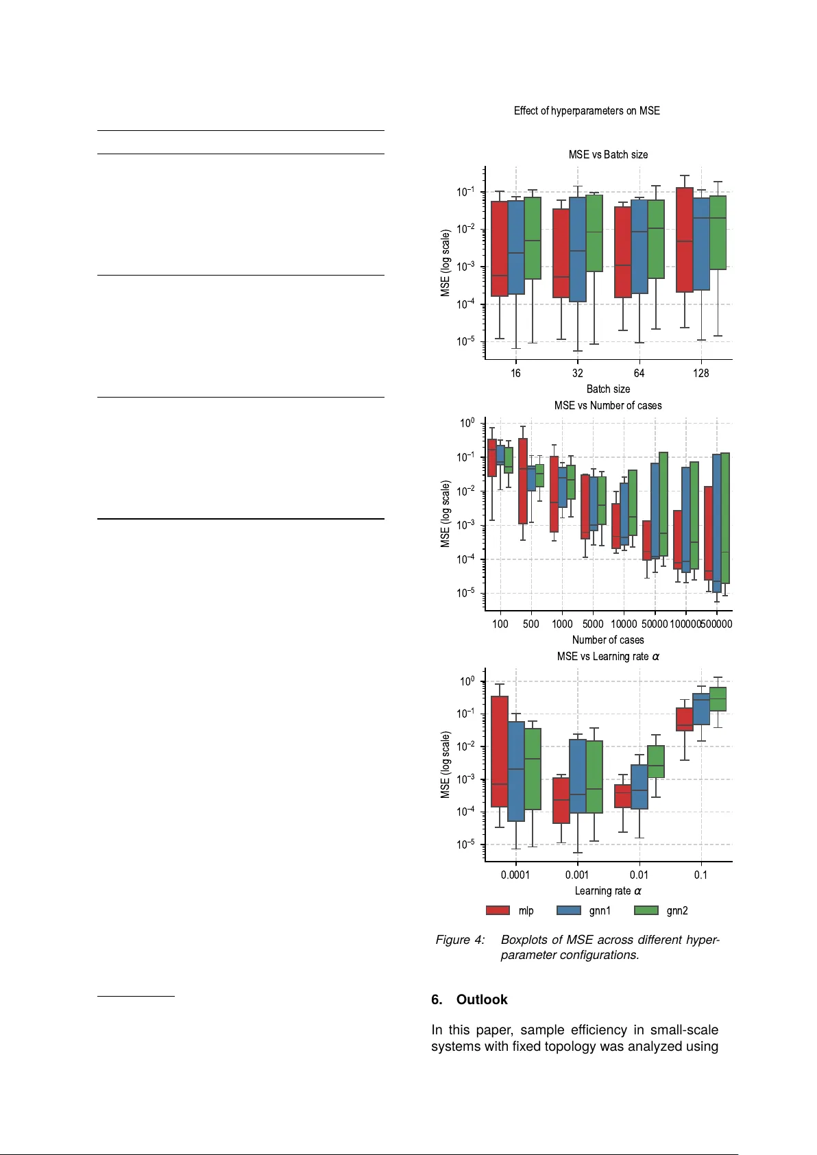
Oberlausitzer Energiesymposium 2025 & Zittauer Energieseminar , Zittau, Deutschland, 25./26. Nov ember 2025 Impact of T raining Dataset Size for ML Load Flow Surrogates Timon Conrad 1 ∗ , Johann Jäger 3 Institut e of Electrical Energy Syst ems, Friedric h-Ale x ander -Univ ersität Erlangen-Nürnber g, Erlangen Changhun Kim 2 , Andreas Maier 4 , Siming Bay er 5 P atter n Recognition Lab, F riedrich-Ale xander -Univ ersität Erlangen-Nürnber g, Erlangen Efficient and accurate load flow calculations are a bedrock of modern power syst em operation. Clas- sical numerical methods such as the NewtonR aphson algorithm provide highly precise results but are computationally demanding, which limits their applicability in large-scale scenario studies and optimiza- tion with time-critical cont exts. Research has shown that machine learning approaches can appro ximate load flow results with high accuracy while substantially reducing computation time. Sample efficiency , i.e. their ability to achiev e high accuracy with limited training dataset size, is still insufficiently researched, especially in grids with a fix ed topology . This paper considers a sy stematic investigation of the sample efficiency of a Multilay er P erceptron and two Graph Neural Networks variants on a dataset based on a modified IEEE 5-bus system. The results for this grid size show that Graph Neural Networks achieve the lowes t losses. Howe ver , the av ailability of large training datasets remains the dominant factor for performance over architectur e. Code: https://github.com/timonOconrad/loadflow- ai 1. Introduction The A C load flow calculation is widely used as a fundamental component of modern power sys- tem operation, par ticularly in the context of con- gestion identification and resolution under frame- works such as Redispatch 2.0. The Newton- Raphson (N-R) algorithm, a classical numerical method, has been extensiv ely employ ed in the solution of non-linear equations of AC load flow . This method is known for its high accuracy , good conv ergence rate and robustness. Howe ver , its computational cost can become prohibitive in large-scale scenario studies or optimization in conte xts requiring rapid responses in large-scale grids. [1] Surrogate models based on Multilay er P ercep- trons (MLPs) hav e been explor ed for sev eral decades. An early contribution was made by [2], who proposed a neural network architecture that emulates the Newton–R aphson method to estimate voltage magnitudes and phase angles. This was followed by a number of fur ther devel- opments that applied MLPs to various load flow applications, e.g. [3, 4]. More recently , Graph Neural Networks (GNNs) hav e been proposed as a more structure-a ware alternativ e to MLPs. GNNs exploit the grid topol- ogy explicitly , modelling buses as nodes and electrical connections as edges. By embedding the power system as a graph, GNNs are capable of lev eraging local and global structural informa- tion through message passing schemes. This architectural property enables improv ed general- ization across varying power injections, par ticu- larly in scenarios where the grid topology is fix ed. Sev eral studies have repor ted that GNN-based surrogates outper form classical MLPs (men- tioned as fully connected networks) in accuracy and training time for small [5] and big [6, 7] grids. In [7], a GNN-based architecture generalized to grids of different sizes (10110 buses) despite be- ing trained only on 30-bus systems. This trans- ferability was not achiev able with MLPs, which failed under varying grid structures due to their fix ed in put vect ors. F ur thermore, the proposed GNN converged faster in terms of iterations and achiev ed a twofold reduction in inference time compared to a commercial load flow solver . Despite promising results in the application of GNNs and MLPs as surrogate models for load flow appro ximation, little attention has been paid to their sample efficiency , especially in fixed- topology settings. While previous work has fo- cused on architectural innov ations and general- ization across topologies or grid sizes [5–7], the relationship between training dataset size and model per formance remains insufficiently under - stood. This paper addresses this gap by presenting a com parison of three neural network architec- tures on a fixed topology . All experiments are conducted on a modified IEEE 5-bus syst em using the same in puts to ensure com parability across models. Oberlausitzer Energiesymposium 2025 & Zittauer Energieseminar , Zittau, Deutschland, 25./26. Nov ember 2025 The results provide a basis for q uantifying sample efficiency in constrained scenarios and using these results to suppor t the development of GNN-based surrogate models when scaling up to larger power grids. 2. Dataset The dataset a used in this work consists of syn- thetically generated load flow cases based on a modified IEEE 5-bus syst em. Each entr y con- tains the full set of load flow results, including voltages in real and imaginar y par t, active and reactiv e powers at each bus. The dataset com- prises a total of 789,000 individual cases, stored in P arquet format for efficient processing. The following section provides a brief ov er view of the data generation process, including the grid model and paramet er variation. Details can be found in the associated thesis [8]. 2.1. Grid Model The grid used in this paper is based on the IEEE 5-bus system, with all line paramet ers and bus configurations identical to those described in the original specification [9]. The only modification is that no load is connected to the PV bus (Bus 2), which distinguishes this model from the standard configuration. The grid topology is illustrated in Figure 1. S Bus 1 PV Bus 2 PQ Bus 3 PQ Bus 4 PQ Bus 5 1–2 1–3 2–3 2–4 2–5 3–4 4–5 Figure 1: Modified IEEE 5-bus syst em used in data generation. S = Slack bus, PV = Gener - ator bus, PQ = Load bus. 2.2. Data Generation The data was generated using AC load flow sim- ulations per formed in DIgSILENT Po werF actor y . For each case, selected in put paramet ers were randomly varied within physically meaningful lim- its. Specifically: a https://github.com/timonOconrad/ static- voltage- stability- AI • Active power at the PV bus (Bus 2) was varied between 0 and 199 MW . • Active power demand at the PQ buses (Bus 35) was varied between 0 and 99 MW . • Reactive power demand at the PQ buses (Bus 35) was varied between 0 and 99 MV Ar . All power values were generated using random sampling and rounded to integer values to sim- plify post-processing. The slac k bus served as a fixed voltage reference and was not modified during the simulations. 3. Architectures 3.1. Graph Neur al N etw ork (GNN) For the proposed GNN, the electrical grid G = ( V , E ) is represented as an undirected graph with |V | = N buses (nodes) and transmission lines (edges). The architecture can be divided into 3 steps: 1. Bus-specific Embedding 2. Propagation (Message P assing) 3. Decoding The architecture is illustrated in Figure 2 and described in more detail below . 1. Bus-type-specific Embedding: Each bus (node) is assigned to a type (slack, PV , PQ) based on the applied grid (subsection 2.1) and the feature vector f i ∈ R 2 b for each bus is con- structed by the type (1). Slack (T ype 1): f i =  V real , V imag  PV (T ype 2): f i =  P , | V |  PQ (T ype 3): f i =  P , Q  (1) Each bus i ∈ V is first mapped into a d - dimensional embedding vector using a bus- specific function (2). h (0) i = ϕ type ( i ) ( f i ) , ϕ : R 2 → R d . (2) All bus embeddings results were collected in the node feature matrix (3) where each column cor - responds to the latent representation of one bus. H (0) =  h (0) 1 , h (0) 2 , . . . , h (0) N  ⊤ ∈ R N × d . (3) b Note: In contrast to the calculation method used by Newton-R aphson, this implementation uses the real ℜ{ V } and imaginar y ℑ{ V } par t of the voltage, to avoid the usage of the voltage angle θ for reasons of normalization. In order to achieve the same vector size R 2 for the slack bus type as for buses with PV or PQ type, the magnitude of the voltage V = | V | was omitted in the feature. As the bus-specific de- coder for GNN1, also requires same vector size R 3 for all bus types, the magnitude of the voltage V = | V | was inserted for the slack. For reasons of comparability , the output vector for GNN2 and the MLP also uses with these vectors. Oberlausitzer Energiesymposium 2025 & Zittauer Energieseminar , Zittau, Deutschland, 25./26. Nov ember 2025 S V real V imag PV P | V | PQ P Q PQ P Q PQ P Q Bus-specific Embedding R 2 → R 100 h (0) 1 h (0) 2 h (0) 3 h (0) 4 h (0) 5 ϕ PQ ϕ PQ H (0) ϕ slack ϕ PV ϕ PQ h (1) 1 h (1) 2 h (1) 3 · · · · · · H (1) h ( k ) 1 h ( k ) 2 h ( k ) 3 · · · · · · H ( k ) w 1 − 2 w 2 − 1 w 1 − 3 w 3 − 1 w 2 − 3 w 3 − 2 w 1 − 2 w 2 − 1 w 1 − 3 w 3 − 1 w 2 − 3 w 3 − 2 Propagation H ( k ) = H ( k − 1) + tanh ( W ( AH ( k − 1) ) W ) P Q | V | Q V real V imag | V | V real V imag | V | V real V imag | V | V real V imag ψ slack ψ PV ψ PQ · · · · · · · · · · · · · · · · · · Bus-specific Decoder R 100 → R 3 Figure 2: Illustration of the architectur e of the GNN Model with Bus-specific Decoder 2. Propagation (Message Passing) The con- nectivity used for message passing is encoded in the adjacency matrix (4). A ij =  1 if ( Y r ) ij  = 0 ∨ ( Y i ) ij  = 0 , 0 otherwise . (4) A ∈ { 0 , 1 } N × N , derived from the bus admittance matrix Y bus = Y r + j Y i . Self-loops are remov ed by setting A ii = 0 . Degree normalization is ap- plied using the diagonal degree matrix ( Equa- tion 5). D with D ii =  j A ij : A ← D − 1 A. (5) Propagation is per formed iterativel y for K steps. At each step, the node feature matrix is updated as in (6). H ( k ) = H ( k − 1) + tanh  ( A H ( k − 1) ) W  (6) The weight matrix W with W ∈ R d × d is a train- able parameter that linearly transforms the ag- gregat ed neighbourhood information before the non-linearity is applied. It ensures that mes- sages received from neighbouring nodes are projected into the same latent space as the resid- ual connection H ( k − 1) . The residual connection stabilizes training and improves gradient flow . 3. Decoding: After k propagation steps, the fi- nal node states { h ( k ) i } N i =1 are decoded into phys- ical predictions. T wo decoder strategies are used, which represent the difference in the two GNN architectur es under consideration: A. Global Decoder (GNN1): Aggregate all bus states by mean pooling ( 7) followed by a feed-forward mapping (8). ¯ h = 1 N N  i =1 h ( K ) i , (7) y = ψ ( ¯ h ) , ψ : R d → R m . (8) This produces the same prediction vector y as for the MLP . B. Bus-specific Decoder (GNN2): Decode each bus separately using type-dependent decoding similar to the embedding step (9). y i = ψ type ( i ) ( h ( K ) i ) , ψ type ( i ) : R d → R m i . (9) The full output is the concatenation of all buses (10). y =  y 1 ∥ y 2 ∥ . . . ∥ y N  . (10) 3.2. Multilay er Perceptron (MLP) As a baseline, a MLP is employ ed. T o ensure comparability with the GNN, the same bus- specific features are concatenat ed into a single input vect or (11) which corresponds to the flattened feature (1) representation of all buses. x ∈ R 10 , (11) The MLP predicts the same set of target vari- ables (12) as the GNN, representing the concate- nated outputs across all buses. y ∈ R 15 , (12) Oberlausitzer Energiesymposium 2025 & Zittauer Energieseminar , Zittau, Deutschland, 25./26. Nov ember 2025 Each hidden lay er of the MLP applies a fully con- nected linear transformation follow ed by a non- linear activation (13) where W and b denote the trainable weights and biases. h ′ = tanh( W h + b ) , (13) The input vector x is thus successively trans- formed into higher-le vel representations, until the final output y is obtained. Unlike in the GNN, where message passing in- corporates the grid topology via the adjacency matrix A , the MLP treats all input featur es as independent and fully connected. The weight matrices W represent connections between all units of adjacent layers, without structural con- straints from the pow er grid. This mak es the MLP a topology-agnostic baseline against which the GNN can be compared. 4. Experiments The experimental study was conducted using the three machine learning architectur es introduced in section 3. The MLP had one hidden lay er with 64 neurons. The two GNNs had for d = 100 and for k = 5 . These parameters were deter - mined initially and showed good results. The objective was to inv estigat e how key hyperpa- ramet ers influence model accuracy in the task of load flow appro ximation for all architectur es. While the training dataset size constituted the primary focus, additional experiments were con- ducted to assess the effects of batch size and learning rate. The paramet ers relating to the ar - chitecture were not adjusted fur ther to enable a comparison. The explor ed hyperparameter con- figurations are summarized in T able 1. T able 1: Hyperparame ter variations e xplored in the e xperiments. Hyperparameter V alues varied T raining size 500, 1.000, 5.000, 10.000, 50.000, 100.000, 500.000 Batch size 16, 32, 64, 128 Learning rate 1 · 10 − 4 , 1 · 10 − 3 , 1 · 10 − 2 , 1 · 10 − 1 All models were trained on the dataset described in section 2. The considered cases were par - titioned into 70% training, 15% validation, and 15% testing splits. Features and targets were standardized using paramet ers derived from the training set. T raining was per formed for a max- imum of 50 epochs using the Adam optimizer . The MLP was trained on flattened input vectors, whereas the GNNs operated directly on per-bus features and the fixed grid topology via the ad- mittance matrix Y . Mean squared error (MSE) 0 10 20 30 40 50 Epoch 1 0 6 1 0 5 1 0 4 1 0 3 1 0 2 1 0 1 MSE loss (log scale) T raining and validation loss (best runs highlighted) MLP T rain (best) MLP V al (best) GNN1 T rain (best) GNN1 V al (best) GNN2 T rain (best) GNN2 V al (best) Figure 3: T raining and V alidation Loss Cur v es. The best configuration for each model is highlighted; all others are displa yed with low er opacity . ser v ed as the primar y loss function. As illustrat ed in Figure 3 and T able 2, GNN1 (global decoder) achieved the lowest validation loss among all models, conver ging to 5 . 66 · 10 − 6 . Howe ver , its training dynamics were less stable, with noticeable fluctuations during early epochs. In contrast, the MLP exhibit ed a smoother and more stable conver gence behavior , ultimat ely reaching a slightly higher but still competitiv e val- idation loss at 1 . 14 · 10 − 5 . It was surprising that the MLP still performed well compared to the GNNs, unlike [5], but this may be due to the fix ed topology and probably no longer works as well with larger grids. GNN2 (bus-specific decoder) positioned itself between these two e xtremes, with validation losses of 7 . 36 · 10 − 6 but a less consistent progression. Ov erall, these results highlight that while GNN1 provides the best final validation accuracy , the MLP demonstrat es the most robust and stable learning behavior across runs. The obser ved variance across runs indi- cates that additional hyperparamet er optimiza- tion (e.g., learning rate schedules, depth, and regularization) will be required to fully exploit the potential of the GNN architectur es. 5. Results The final test using the test dataset T able 2 shows comparable results to those of the vali- dation dataset, with the GNN1 model proving to be the most effective architecture. The results shown in Figure 4 indicate that the training dataset size had the largest and most consistent effect on prediction accuracy across all models. As the number of training samples increased, Oberlausitzer Energiesymposium 2025 & Zittauer Energieseminar , Zittau, Deutschland, 25./26. Nov ember 2025 T able 2: T op-3 runs per model ranked by low est final v alidation loss. MLP GNN1 GNN2 Run 1 Learning rate 0.001 0.001 0.0001 Batch size 32 32 32 Cases 500k 500k 500k T rain (MSE) 1 . 25 · 10 − 5 1 . 05 · 10 − 5 1 . 31 · 10 − 5 V al (MSE) 1 . 14 · 10 − 5 5 . 66 · 10 − 6 8 . 55 · 10 − 6 T est (MSE) 1 . 14 · 10 − 5 5 . 65 · 10 − 6 8 . 51 · 10 − 6 Run 2 Learning rate 0.001 0.001 0.0001 Batch size 16 16 16 Cases 500k 500k 500k T rain (MSE) 1 . 47 · 10 − 5 1 . 06 · 10 − 5 8 . 92 · 10 − 6 V al (MSE) 1 . 18 · 10 − 5 6 . 49 · 10 − 6 9 . 17 · 10 − 6 T est (MSE) 1 . 18 · 10 − 5 6 . 51 · 10 − 6 9 . 15 · 10 − 6 Run 3 Learning rate 0.001 0.0001 0.001 Batch size 64 32 16 Cases 500k 500k 500k T rain (MSE) 1 . 87 · 10 − 5 9 . 31 · 10 − 6 2 . 04 · 10 − 5 V al (MSE) 2 . 00 · 10 − 5 7 . 36 · 10 − 6 1 . 28 · 10 − 5 T est (MSE) 2 . 01 · 10 − 5 7 . 36 · 10 − 6 1 . 28 · 10 − 5 the test loss decreased notably and the variance across runs was reduced. Batch size had negligible influence on model performance. While no consist ent trend for learning rate was obser ved for GNN1 and the MLP , GNN2 e xhibited a strong correlation between learning rate and test loss, suggesting that smaller learning rates improv ed its stability and final accuracy . Figure 5 shows the inference time c of the considered models in comparison to an N-R solver d . The lowest com putation times are obtained by the MLP , which remains below 0.35 s for 10,000 samples due to its simple architecture. The GNN variants require about 34.6 s (GNN1) and 38.3 s (GNN2) for the same number of samples, while the N-R solv er requires about 142.5 s. This corresponds to a speedup of about four for the GNNs and more than four hundred for the MLP compared to N-R. For small sam ple sizes the advantage of the neural models is less pronounced, as the fix ed ov erhead of the GNNs dominates, whereas for larger case studies the advantage becomes much more significant. c Windows 11 machine with an Intel Xeon Gold 6226 CPU (16 cores), 10.4 GB RAM, Python 3.9 & without GPU suppor t d parallelised implementation, one case was solved re- peatedly 16 32 64 128 Batch size 1 0 5 1 0 4 1 0 3 1 0 2 1 0 1 MSE (log scale) MSE vs Batch size 100 500 1000 5000 10000 50000 100000 500000 Number of cases 1 0 5 1 0 4 1 0 3 1 0 2 1 0 1 1 0 0 MSE (log scale) MSE vs Number of cases 0.0001 0.001 0.01 0.1 L e a r n i n g r a t e 1 0 5 1 0 4 1 0 3 1 0 2 1 0 1 1 0 0 MSE (log scale) M S E v s L e a r n i n g r a t e Ef fect of hyperparameters on MSE mlp gnn1 gnn2 Figure 4: Boxplo ts of MSE across different h yper - parame ter configurations. 6. Outlook In this paper , sample efficiency in small-scale syst ems with fixed topology was analyzed using Oberlausitzer Energiesymposium 2025 & Zittauer Energieseminar , Zittau, Deutschland, 25./26. Nov ember 2025 1 0 0 1 0 1 1 0 2 1 0 3 1 0 4 Number of Samples 1 0 2 1 0 3 1 0 4 1 0 5 Computation T ime (ms) Inference T ime MLP GNN1 GNN2 Newton-Raphson Figure 5: Infer ence time depending the number of samples on the best models (Run 1) or N-R algorithm three neural network architectures. It was shown that larger training datasets result ed in lower MSE, an effect expect ed to become even more critical in larger power grids, as dataset genera- tion becomes increasingly time-consuming. Fu- ture work will therefore focus on the integration of phy sics-informed loss functions, as in [11], which explicitly incor porat e domain knowledge through known physical relationships, as well as on the application of Known Operator Learning. These approaches are expected to mitigate the dependence on large training datasets. According to [7], GNNs are par ticularly promis- ing in this regard, as they enable deployment in larger power grids without extensiv e retraining and reduce the need for large training datasets. The analysis of this capability and its applicability to larger grids will be par t of future work. Acknowledgment This work was conducted within the scope of the research project GridAssist and was suppor t ed through the OptiNetD funding initiative by the German Federal Ministr y for Economic Affair s and Energy (BMWE) as par t of the 8 th Energy Research Programme. References [1] P . Kundur , P ow er Syst em Stability and Con- trol , McGraw-Hill, pp. 255–267, 1994. [2] T . T . Nguyen, “Neural network load-flow , ” IEE Proceedings - Generation, T ransmission and Distribution , vol. 142, no. 1, 1995. IET . [3] V . L. Paucar and M. J. Rider , “ Ar tificial neural networks for solving the load flow problem in electric power systems, ” Electric Pow er Sys- tems Research , vol. 62, pp. 139–144, 2002. Elsevier . [4] T . Pham and X. Li, “Neural Network - based load flow model, ” 2022 IEEE Green T echnologies Confer ence (Green T ech) , 2022. IEEE. DOI: 10.1109/GREEN- TECH52845.2022.9772026. [5] Y . Lin, E. Orfanoudakis, M. Welzl, and L. Roald, “PowerFlo wNet : Graph neural net- works for load flow prediction, ” arXiv preprint arXiv :2311.03415 , 2023. [6] M. Lopez-Garcia and J. Domínguez-Nav arro, “load flow analysis via typed graph neural net- works, ” Engineering Applications of Ar tificial Intellig ence , vol. 117, ar t. no. 105567, 2023. Elsevier . [7] B. Donon, B. Donnot, I. Guyon and A. Marot, "Graph Neural Solver for P ower Syst ems," 2019 International Joint Conference on Neu- ral Networks (IJCNN), Budapest, Hungar y , 2019, doi: 10.1109/IJCNN.2019.8851855. [8] T . Conrad, AI-Based Static V oltage Stabil- ity Analy sis of Po wer Grids , Master’ s thesis, Hochschule Zittau/Görlitz University of Ap- plied Sciences, Zittau, Germany , Sept. 2023. [9] A. A. Bhandakkar and L. Mathew , “Real- Time-Simulation of IEEE-5-Bus Network on OP AL -RT -OP4510 Simulator , ” IOP Confer - ence Series: Materials Science and Engi- neering , vol. 331, no. 1, p. 012028, 2018, doi:10.1088/1757-899X/331/1/012028. [10] C. Croux and C. Dehon, “Influence func- tions of the Spearman and Kendall cor - relation measures, ” Statis tical Methods & Applications , v ol. 19, pp. 497–515, 2010. Springer . [11] L. Böttcher , H. Wolf, B. Jung, P . Lu- tat, M. T rageser , O. Pohl, X. T ao, A. Ul- big und M. Grohe, "Solving AC load flow with Graph Neural Networks under Realis- tic Constraints," 2023 IEEE Belgrade Po w- erT ech, Belgrad, Serbien, Juni 2023, doi: 10.1109/powertech55446.2023.1020224.