The impact of class imbalance in logistic regression models for low-default portfolios in credit risk

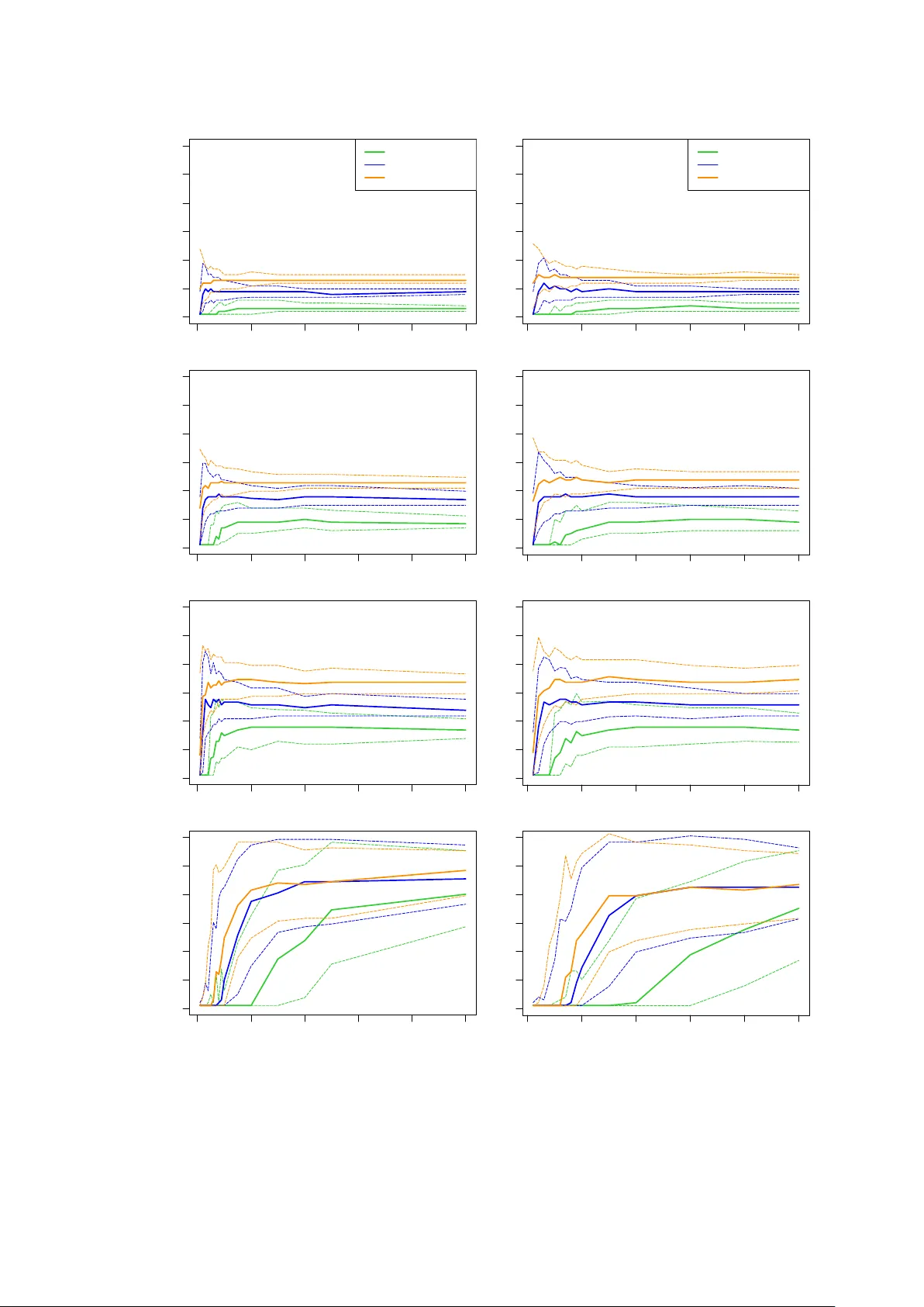
1 The impact of clas s imbal ance in logistic regression mode ls for low - default portfolios in credit ri sk Willem D Schu tte 1,2 , Charl Pretor ius 1,2 , Neill Smit 1,2 , Leand ra van der Merwe 1 , Robert Maxwell 1 1 Centre for B usine ss Mat hematic s an d Info rmatic s & Unit f or Dat a Sci ence and Comp uting, Nor th - West U nive rsit y, South Afric a 2 National Ins titute fo r Theoreti cal and C omputatio nal Ph ysics (NITh eCS), Pot chefstroo m, South Afr ica 23 February 2026 Abstract In this paper , we stu dy ho w class imbal anc e , typic al of low - de fault cre dit portf olios , affects th e perfor mance o f logi stic regres sion models . Usin g a simul ation s tud y with c ontro lled data - gener ating me chanis ms, we va ry (i) the le vel of class i mbalanc e and (ii ) the stren gth of associa tion between the pr edictor s and th e respon se. The resu lts show that, for a give n stre ngth of associa tio n , achievab le classific ation accurac y deteriorat es markedly as the event rate decrea ses, a nd the opti mal c lassific ati on cut -o ff shift s wit h th e level o f im balanc e. In contra st, the Gi ni co effici ent is co mpara tivel y sta ble w ith r espec t to class imbal anc e onc e sa mple s ize s are suff icie ntl y larg e, ev en whe n classific ati on a ccura cy is stron gly a ffec ted. As a practical gui de lin e , we summ arise attaina ble cl assific atio n perfor mance a s a func tio n of the e vent ra te and st reng th o f asso cia tion bet ween t he pred icto rs an d the resp onse . Key wor ds: Cl ass imba lance ; Clas sifica tion; Conco rdance; Credit ri sk ; Cr edi t scorec ards ; Gin i coeffic ient; Logi sti c regre ss ion ; Weight o f evi denc e 1 Introduction The estimati on of the ris k para meter s fo r por tfoli os th at e xhibit a low - defaul t na ture po ses a commo n chall eng e for financial ins tituti ons wo rld wide. For t hes e type s of portfo lio s, typically referre d to a s low - defa ult p ortfoli os (LDPs), defa ult events are ve ry l imited and extr emel y unde rrep re sent ed in the da ta, causing the ev ent and none vent clas ses to be im balanced . Such data sets a re s aid to exh ibi t class im balance . When bank s de ve lop m odel s fo r r isk p arame te rs base d o n LDP s , it is not kn own pre ci sely wha t impa ct the c lass im bal ance pro blem wi ll hav e on aspect s of the m odel perfor manc e , such as the acc uracy of predicti ons , the discrimi nation 2 ability of t he mod el, an d c lassific atio n cut - o ffs . It is al so kn own th at re gu lators prefe r model s to be deve loped on real client dat a rathe r than simulate d d ata . When usi ng lo gistic re gressio n in c lassifi catio n pro ble ms , it is well d ocume nted th at c lass imbalance ca n have det rim ental eff ects , inclu ding a low cla ssific ation accu racy for t he mi nority cla ss, we ak sep arat ion ab ili ty of the class if ier , and unde rest ima tion of th e pr obab ili ty of a ra re even t. S tanda rd cla ssifi ers are often biase d toward s the maj ority class and c onse quentl y ha ve a higher misc lassi ficati on r ate f or th e mi nority cla ss ( López e t al., 2013 ). F urthe rm ore , the choi ce of perfor mance metric guidi ng t he lear ning pro ces s might induc e fu rther bia s if the p er form ance metric do es no t adequate ly penalise miscla ssific atio n of th e minorit y cla ss ( Haixiang et al., 2017 ). Zhang et al. (2018 ) sh ow that , when tra ined on he avi ly imb ala nce d da ta se ts, l ogi stic reg ress ion can yield a very smal l false ne gative rate while having a very h igh fa lse pos itiv e ra te . A numerica l study b y Zhang et al. (2018) i ndi cates tha t t he separation ability , as meas ured by the Kolmog orov - S mirno v stati stic, of the log isti c re gress io n clas sifier c an be sensi tive to a low e vent rate . Th is cou ld be c a use d by min ori ty clas s obse rva tio ns ov erl app ing wi th major ity class obse rv ation s ( Haixiang et al., 2017 ). A ccord ing to King and Zen g (200 1) , appl yin g log ist ic reg ress ion to small samp les ca n le ad to undere stim ati on of the p rob abil ity o f t he r are eve nt . In the case of a more s eve re class i mbal ance in the d ata se t , a gre ate r bi as i n the pred icte d probabilities can be e xpect ed ( Puhr et al., 2017 ). It shoul d be noted that studi es t hat inv es tigat e the eff ects of c lass imba lance ar e typic ally based on real data s ets. Th ere is a cl ear lack o f controll ed simu latio n stu dies to prop erly evaluate the impac t of im balanced data, es pecially i n the cre dit ri sk e nviro nmen t. There exist se veral r emedi al measur es to add res s ad verse effec ts i ntro duc ed by the c lass imbal ance pr oblem. It is appa rent from the surv eyed l itera ture that it is stil l unc lea r whic h combin ation of classi fic ation mo del an d remedial meas ure is most approp riate in a giv en situat ion (see , e.g ., Jiang et al., 2023 , van den Goo rbe rgh et al. , 202 2 , X iao et al., 2021 , López et al., 2013 ). W e br ie fly desc ri be four catego ries of remed ial mea sures: resam pli ng a ppro ache s, synthes ising techni que s, em bedde d fram ework approac h es , and p ost - hoc adjust ment method s. T his t axo nomy is propos ed by Jiang et al. (2023) , wh i ch is a ref ineme n t of wha t is usua lly refe rred to as da ta - le ve l tech niq ues and algor ith m - level techniq ues ( see, e.g ., Rout et al., 2018 ). Res amp ling a ppro ac hes inv olve res amp ling the dat a to re duce c la ss imb alan ce at a data le ve l. Pop ular tec hniq ues i nclud e ra ndom o ver - samp ling, rand om unde r - sampli ng , and ad apte d version s of these two tec hnique s ( see Jia ng et a l., 202 3 ) . Resa mpling ap pro aches a ppear to be the mo st po pular i n cr ed it scori ng a pplic ations, mo st li kely due to the simp licit y and ease of implem entati on. Howe ver, t here a re con tradict ing re sults on th e effic acy of re sam pling app roa ches i n the lite rat ure , and mos t stud ies ar e based on real d ata se ts ins tea d of cont rol led sim ulat ion s sett ing s . Kim and Hwang (2022) sh ow tha t resam pling t echniqu es ca n be inef fectiv e in impr oving a classif ier’ s perf orma nce an d can in so me ca ses als o be detri mental. van d en Goorbergh et al. (20 22) show that, after c orrecti ng for c lass i mbala nce, the prob abili ty of 3 belongin g to th e minori ty class is s ignifi cantl y o veresti mate d. Mar qués et al. ( 2013) demo nstra te that usi ng r esa mplin g me thods l eads to a co nsist ent i mprov ement in mod el per forma nce, w ith over - samp ling per form ing b ette r th an a ny und er - sampling ap proach. A r elabelli ng approach wa s recent ly prop osed by Li ( 2020) , where the au thor show s that resam pling t he mi nority class i s insuffi cient for handli ng th e class imbal anc e pro blem and d emonst rates that the prop osed relabell ing a pproac h i s m ore eff ectiv e in captu ring the u nde rlying struc ture of th e mino rity c las s. Synt hes isi ng techni ques are used to g enerat e additio nal minority c lass observ ati ons us ing mecha nisms tha t avoid the repeti tion or dup li c at ion of entrie s from the m inori ty c lass. Popular synthes ising t echni que s include synthe tic minority ove r - sampli ng techn ique ( S MO T E; se e Chawla et al., 2002 ) and its v ari ous ex te nsion s , g ene rat ive a dver sar ial ne two rks ( GA Ns; see Goodfellow et al., 2014 ) , and the adapt ive synth eti c sampli ng meth od ( ADASYN; see He e t al., 2008 ). Embedd ed fra mew ork a pproac hes ref er to tech niqu es that involve i nte gratin g resa mpling method s or synth esisi ng t echniqu es i nto existi ng model - build ing appr oac hes not i nhere ntly suita ble for c lass - imbalanc ed dat a . Two exa mple s are th e sam pling - embe dded ap proa ch , which involv es combi ning, fo r exam ple, unde r - sam pling w ith ba ggin g or S MOTE w ith boos ting , and t he cost - embedded app roach , wh ich combi nes resam pli ng app roa che s wit h cost - sens it ive le arni ng where misclassi fica tions are pe nalise d accor ding to the sev erity of the con seque nce of suc h misclas sifica tions. Jiang et al. (2023) mention tw o pos t - hoc adju stin g m ethods: thresh old adju stin g and M etaCost . Thre sho ld ad jus ting involves mod ify ing the clas sifi cation c ut - off to minimise the tot al cost o f mis class ify ing obse rvat ion s. This a ppro ach is a ppropri ate w hen the cost of miscl assifi catio n is asymm etrical , e.g. , when the cost of ap provi ng a l oan to a cust omer w ho i s lik ely to def ault i s greater than t he cost of not a pprovi ng a loa n to a custo mer who i s likel y to no t defaul t. For a descri ption of Meta Cos t , which is rela ted to cost - sensiti ve cl assi ficati on, see Domingos (1999) . Beside s the ev ent rat e, whi ch López et al. (2013) indic ate as the m ain f acto r affecti ng cla ssi fier perfor mance, most studies find that ot her pr ominen t fact ors suc h as sample siz e, numb er of predic tors, a nd numbe r o f even ts p er pre dictor vari able also i nflu ence mod el per form ance. The reader i s ref erred to López et al. (20 13) for furth er d iscussi ons on c las sific ation p robl ems in th e presenc e of a low ev ent rate. It is expec ted tha t the n umber of observ ations avai labl e for trai ning a mod el wi ll af fect i ts perfor mance. In c ontra st to th e rela tiv ely sma ll sa mple sizes typic ally reco mmend ed for cr edit scoring app licati ons ( see, e.g., Siddiqi, 2017 ) , Crone and F in lay (2 012) ad voca te the use of samples con tainin g at l east 1 500 to 2 000 ob serv at ions. T rad ition al maximum lik elihoo d estimati on is know n to have pot entiall y pr oblema tic small - sam ple b eha vio ur ( van S meden et al., 2019, lists fi ve spec ific issues ) . As a reme dy, van Smede n et al . (2019) s hows that reg ress ion shrink age can alle viate th ese adve rse effec ts. The y also sug gest that t he requi red sa mple si ze for a given situ ation shou ld be deter mined acco rding to out - of - s ampl e pr edic tiv e perfo r manc e. 4 Based on a simula tion st udy in volvin g resam pling from clinical trial dat a, Peduzzi et al. (1996) showe d that for si tuati ons wh ere the nu mber of minori ty - class e vent s pe r pre di ctor vari able , o r simpl y refer red to a s ev ents pe r varia ble (EPV) , was le ss th an 10 , the regre ss ion c oef fici ent s were biased i n both direc tio ns and th e sample varianc e s of the e stima ted c oeffici ents w ere overes timat ed. In fact, several othe r aut hors su ggest a n EP V of at leas t 10 (s ee, e .g., Harrell Jr et al., 1985 , Wynants et al., 2015 ) , a nd Freed man and Pee (1989) showe d tha t an EP V o f less than 4 leads to incre ased ov erfitti ng. In contrast to th ese fi ndings, van Smeden et al. (2019) fo und t hat EPV doe s not h ave a str ong r elation w ith metric s of predic tive perform ance. The y claim t hat E PV is not a su itabl e criteri on for binary predicti on mo del dev elop ment. Instea d, the y recomm end consid ering the nu mber of p redict ors, the to tal sa mple size , and th e eve nt ra te. It is expec ted that c ertai n pr edicto rs w ill c ontai n mo re pre dicti ve valu e about the even t th an ot her pre di ctors . In add ition , eve n if sev er al pre dict ors a re comb ined i n a mode l, ther e wil l sti ll be an unobse rved error com ponent cau sing unex plain ed var iabi l ity in t he true outco me . If the er ror variabil ity is so l arge that it ob fusca tes the info rm ation c ont ained i n the pr edictor s, the noi se (err or ) is more p romi nent th an the sign al (p redi ctor s) , and we say that the re i s a low si gnal - to - noise rati o . If the err or is ne gligibl e an d the p redict ors c ontain clea r inf ormati on rega rdin g the outc ome, w e h ave a hi gh signal - to - noise r atio. T o ou r know ledg e, the re exist s no lit era ture on the ef fect of th e signal - to - no ise r atio in t he ca se of c lass imba lance. Mo st li teratu re focus es o n pr oxies su ch a s EP V me ntio ned abov e. In this p aper, w e con sider the im pact of c lass i mbal ance i n logis tic reg ressi on mod els fo r credi t risk in a c ontr olled simul ation stu dy setup. S ever al simu lation c onf igurati ons are con side red under differe nt le vels of class i mbal anc e. I n line with the find ings o f van Smeden et al. (2019) , we consid er as crit eria for pr edictiv e perfor manc e the sa mple size and event rate . However, we use an agg reg ate i nfo rmat ion val ue (A IV), which t akes i nto a ccou nt the n umber of pred ict ors an d predic tive va lue of each pr edicto r, to captur e the si gnal - to - noi se ratio . No r emed ial meas ure s are appli ed, since the goal of t his s tudy is to eval uate th e im pact o f cla ss im balanc e in t his con text . We will al so show , when usin g imbal ance d traini ng dat a set s, trai ning sa mples shoul d be l arge enough , a s advoca ted by Crone and Finlay (2012) . The rema inde r of th e pap er is st ructu red as f ollow s. In S ecti on 2 , we d iscuss seve ral method ologic al co nsid erati ons, incl uding prel imin aries for the s imu lation stu dy and perfor mance m etrics. Secti on 3 descri bes th e si mulatio n se tup ta ilor ed to be r eprese ntati ve of typical imbala nced data found in c redi t risk modell ing , w ith t he resu lts of the si mulatio n stu dy provide d an d di scuss ed i n Secti on 4. In Sec tion 5, we prese nt p ractic al gu ideli nes, c losi ng rema rk s, and rec ommen dation s for futur e res earch. 5 2 Method ological fra mework 2.1 Model ling prel imin aries In credit scor ing , i t is comm on pra cti ce to dis cret ise co nti nuo us pred icto r vari able s into d iscre te bins . Suppos e tha t we have  d is crete (o r “b inne d”) pre di cto rs, d enot ed b y   ,  = 1, … ,  , which may b e related to th e outc ome of an event. T he ev ent i ndicato r vari able  has mass func tion  (  =  ) =    ( 1    )  ,   { 0, 1 } , whe re    ( 0, 1 ) denote s the ev ent rate . That is,   denot es the proba bility tha t the event  = 1 occurs. Also defi ne t he noneve nt rate   = 1    . A comm on ap proach i n c redit risk mod elli ng i nvolv es usin g w eights o f e videnc e ( see, e.g ., Siddiqi, 2017 ) . The we ight of evi den ce of a predic tor me asure s the st reng th of a pre dic tor in dist ing uish ing bet wee n eve nts and nonev ents . The weig ht of evide nce as soci ated wi th th e eve nt   =  is define d by   (  ) = ln     =    = 0      =    = 1  . (2.1 ) The quantity in (2.1) i s unk nown and is ty picall y estimated using the adjus ted estima tor    (  ) = ln  #    =  ,  = 0  +   # (  = 0 )   #    =  ,  = 1  +   # (  = 1 )  , whe re # (  ) denote s the nu mber of times the event  occ urred in t he sa mple , and  i s a n arbitra ry adjust ment factor inco rpor ated to avo id the est ima tor be ing undef ined whe n #    =  ,  = 1  = 0 . Thro ugh out, w e cho ose  = 0.5 because thi s is t he d efault c hoic e in SAS and there fore used by many pr actiti oner s ( see SAS Institute Inc., 2018, p. 1097 ). The id ea unde rlyi ng t he u se of weight of evide nce is gr ound ed in the re latio nship betwe en conditio nal probabi litie s and odds , whi ch will now be p res ented brie fly . For a more detai led discus sion on th e use o f weight s of evi dence in th e c ontext of cr edit scorec ards, t he reade r can consul t Thomas (2009) . Typ ical ly , one woul d mode l the re lati onsh ip bet wee n  an d  using a l ogistic re gressi on model where the respon se vari able is the condition al log od ds of the eve nt  = 1 gi ven  =  , that is, logit  (  = 1 |  =  ) = ln  (  = 1 |  =  )  (  = 0 |  =  ) . Invoki ng Bayes’ ru le , and a ssuming that th e  comp onents of  = (   , … ,   ) are conditi onal ly inde pende nt (co nditi onal on  ) , th e condi tio nal log odds can be wr itte n in te rm s of the we ight s of evidenc e as 6 logit  (  = 1 |  =  ) = log  (  = 1 )  (  = 0 ) + log  (   =   |  = 1 )   (   =   |  = 1 )  (   =   |  = 0 )   (   =   |  = 0 ) = logit  (  = 1 )            . (2.2 ) This show s that, giv en at tri bute s  =  , the conditi onal l og odds of obs ervin g  = 1 i s pe rfe ctly negativ ely co rrelat ed wi th th e w eight of e videnc e corr espo nding t o th e eve nt  =  . Th is me ans that , giv en  =  , greater v alue s of th e wei ght of evide nce are associate d wi th low er cha nces of obse rv ing the even t  = 1 . In pr actice , it is possi ble that the pre dictor s are not i ndepe ndent . As a n alt ernati ve app roac h , logit  (  = 1 |  =  ) coul d be modell ed usin g th e more gen eral logi stic r egressi on model  (  ;  ) =   +          ,    (2.3 ) whe re  = (   , … ,   ) is an unk no wn p aram ete r ve ctor to be estim ated fro m data. 2.2 I nformat ion value For each  = 1, … ,  , a ssume tha t the r egresso r   can ta ke on one of   possible values (“bins” )   , … ,    . The inf or mati on va lue (IV) associ ated w ith   is defined as       =       =     = 0       =     = 1           ,  = 1, … ,  . (2.4 ) Hig her va lues of   (   ) means that the attri bute   carries i nform ation on the distr ibuti on of the even t  . Note that i f   and  are inde penden t, the n   (   ) = 0 . The inf orma ti on v alue origin ates from in form ation the ory and is re late d to rel ati ve S han non e ntr opy ( Sha nnon, 19 48 ) , al so k nown as the Kullback – Leib le r d ive rge n ce ( Kullback and Leibler, 1951 ). For this stu dy , it will a lso be of i nteres t to d etermi ne the distri buti onal i nformat ion on  that can be d eter min ed fro m kn ow ledg e of a vector of predictors  = (   , … ,   ) , and v ice v ersa. T o this end , we def ine the aggr egate infor mation val ue (AIV) associ ated wi th  by   (  ) =  󰇩 󰇡  |  (  | 0 )    |  (  | 1 ) 󰇢 ln   |  (  | 0 )   |  (  | 1 ) 󰇪  , (2.5 ) whe re  d enote s the set of possi ble v alues o f  . Throughou t th e pape r , the A IV rep rese nts the deg ree/ str engt h of a sso ciat ion betwe en th e resp onse var iab le  and a se t of predic tors  = (   , … ,   ) . U nder con dit ion al inde pen denc e of the co mpo nents of  give n  , it foll ow s that   (  ) =           , wit h   (   ) as defi ned in (2.4 ) . Tha t is, if the pr edicto rs a re c ondi tionall y indepe ndent of o ne anoth er, the AIV is sim ply the sum of th e in div id ual IVs . Rem a rk. T he i nfo rmat ion va lue s defi ned in (2.4) and (2.5) are re lat ed to the p opu lat ion stab ili ty inde x freque ntly u sed in cre dit scori ng in the se nse tha t the y are also sy mmetri sed version s o f 7 the Kullbac k - Le ible r d i stan ce ; see, e.g., L ewis (1994) , Potgie ter e t al. (20 25) , Siddiqi ( 2017) . Howev er, w hile the po pula tion s tab ility index is typ ical ly use d to com pare the deve lopment pop ula tion with the testing popula tion, our focus he re is on c ompa ring, for e ach pr edict or, i ts conditio nal d ist ribu tion w ith in the e ven t clas s to its conditio nal dis tri buti on wi th in the n oneve nt class. 2.3 Performance metric s 2.3.1 Classifica tion m etrics Classific ati on m etrics, also refe rred to a s thre sho ld - de pende nt met rics , are a class o f perfor mance metrics deri ved from the con fusio n matrix ; T able 1 shows a confus ion ma trix for binary cla ssifica tio n proble ms . After re viewing exis ting lit eratur e on c lassi fic ation metrics and their u se in credi t risk mo dellin g, w e consi der onl y two cla ssific ation metr ics in thi s pape r. Table 1 . Bin ary conf usion m atri x. Predicted Positive Negative Actual Positive True positive (TP) False negative (FN) Negative False positive (FP) True negative (TN) The   score is one of the most wi dely used c las sifica tion m etrics and is giv en by th e har monic mea n of re cal l and preci sion, which c an be sim plifi ed to   score = 2 TP 2 TP + FP + FN . The   score ha s b een exte nsivel y us ed i n stu dies wi th cla ss i mbalanc es, but rece nt r esearc h has in dicate d tha t th e metric mi ght no t alw ays be ap propri ate i n cer tain c ase s of c lass imbala nce. T his is o f cou rse eviden t fro m the de finitio n of th e metr ic, w here equ al weig ht s ar e assign ed to recal l a nd pr eci sion. R ecal l re prese nts t he pro portio n of corr ectl y predic ted posi tives out of th e actua l posi tives, wher e prec ision r epr esents t he prop ortio n of c orrectl y pre dicted positi ves out of all p redic ted po sitiv es. Th e   score th us foc uses only o n correc tly cla ssifyi ng th e positi ve clas s, wh ich i s t ypical ly the mino rity cl as s repr esen ting d efault s in the credi t sc oring environ ment. Si nce t he c ost o f an i ncor rec tly cl assif ied de fau lt is ty pi call y much h ighe r than the cost o f an incorr ectly c lassif ied non - d efault, the   score should st ill be a sui ta ble metri c for measur ing cla ssifie r perfor mance on imbalanc ed c redit da ta. The   score , r ecentl y pro posed by Sitarz (2023) , is a more compr ehensi ve m etric for handli ng imbalanced data. The   score i s a sym metrical ext ensio n of th e   score a nd is giv en by th e harmoni c mea n of the rec all, pr ecisi on, spec ifi city, an d nega tive pre dicti ve valu e, whi c h simpli fies to   score = 4 TP × TN 4 TP × TN + ( TP + TN )( FP + FN ) . 8 Consi dering t he d efini tion of thi s metric , e qual w eight i s giv en to the c ost o f miscl assif ying both the posi tive and negativ e cla sses. The   score al lows for label switc hing and its lev el of interpr etabili ty i s si mila r t o tha t of the   score. Sitarz (2023) sta te s t hat th e   score pe nalis es more stron gly than ot her com prehen sive classifi cati on metrics suc h as the M atth ews corr elati on coeffic ient ( MCC ) . Furth erm ore, a w eight ed v ersio n of the   score c ould also be co nsi der ed (similar t o a we igh ted ve rsi on of the   score) to give mo re wei ght to the clas s of i nteres t. T his is rela ted to c ost - based appr oache s, wh ich can m ore he avi ly pena lise m isc lass ifi cat ion of th e class of inte rest. In credi t risk mo del ling , the positi ve cla ss (the event cla ss corresp ondin g to d efaul ts ) i s alway s the min ority cla ss an d cla ss of inte rest, thu s both th e   score a nd   score c ould be appropria te as classi fica tion metric s . 2.3.2 Discrimin ation ability The Gini c oe ffici ent is a popu lar m easur e used in cr edit sc orin g to a ssess the degree of concor dance betw een p redictio ns of the pr obab ili ty of def ault ob tai ned fr om a c las sif ie r and the actual occu rre nce of the defau lt event. That is, g iven tw o custome rs , a classi fier wi th a hi g h Gini score will in mo st cases b e able to cor rectly iden tify whic h of t he two c usto mers are more like ly to default. The Gini co efficien t is t herefo re useful whe n rankin g custo mers is mo re imp ortant than predic tin g wheth er the cu stom er will actuall y defau lt or not. The Gini coe ffici en t , al so know n as Some rs’  ( see, for exa mpl e, New son, 20 02 ), can be used to measur e the degre e of conc orda nce b etwe en  predicti ons    , … ,    obtained fro m a fi tted logistic reg ressi on mod el and t he co rres ponding tru e respon se s   , … ,   . The Gin i coef fici ent o f   with resp ect to  is defin ed b y    |  = (      )    , wher e   is the nu mber of c onco rdant pai rs,   is the nu mbe r of discor dant pairs, an d   is the numbe r of pairs with dif fer ent respons es (i. e., not tied in th e resp onse). If al l pair s in the sample are conc orda nt, th en t he Gi ni coeffic ient i s equ al to 1. I f all pairs are discor dant, then t he Gi ni i s equa l to ‒ 1. We finall y menti on that t he Gi ni co effici ent i s close ly rela ted to the rank - base d cor rel atio n mea sure kn own as Kendall’s tau ( Kendall, 1938 ) . Fo r more detail s on this relat ion, t he interested reader i s re ferred to N ewson (2002) . 3 Simulati on setup 3.1 Simulation pro cedure We con duct a Mont e C arlo si mulat ion con sisti ng of 5 00 M onte Carlo ite ration s for each configuration. The sample sizes considered are 50, 100, …, 450, 500, 750, 1 000, 1 500, 2 000 and 2 500. Fi xed event rates of 1 %, 5%, an d 10% are consi der ed to i nves tigat e the effec t of class imbala nce o n cla ssific ation accu racy. 9 We now outli ne the procedu re to g enerat e a sam ple of siz e  with a spec ifie d numbe r o f even t cases , say   =      , so that the e vent ra te is   . To d o this , set the fir st   respon ses   , … ,    equal to 1 (eve nt ca ses) an d t he rema ini ng     respo nses     , … ,   equal t o 0 (non event cases). Fo r e ach resp onse   ,  = 1, … ,  , genera te a  - dimensio nal vec tor of pr edictor s   = (   ,  , … ,   ,  )  fro m the c las s - conditi onal pro babili ty dist ribu tion  (  =  |  =   ) . The sample , which we d enot e by (  ,  ) , then co nsist s of the design matr ix  = (   , … ,   )  and the re spon se ve ct or  = (   , … ,   )  . Seein g that the cla ssifi er is a logis tic re gressio n model which pr edicts an eve nt proba bili ty, and we are intere sted in cla ssi fying o bser vation s a s an event or a n oneve nt, a classi ficati on c ut - off point   ( 0,1 ) needs to be cho sen. Thi s cu t - off point is chos en by maxi misin g the clas sificatio n accuracy according to some cla ssific atio n metri c , which we choo se to be e ither t he   scor e or the   score as defined in Secti on 2.3.1 . Giv en a c ut - off point of  , we denote b y   (   |  ) the val ue of t he chose n cl assif ica tio n metr ic ca lcul ated using the p red icte d pr oba bil itie s   and the actual binar y obse rv ations  . T he steps follow ed in each Mo nte Ca rlo ite ration are list ed below . T he st eps a re also outl ined visually in Figure 1. 1. Genera te a t ra ining sam ple (  train ,  train ) , a valida tion sam ple (  val ,  val ) , and a tes t sam ple (  test ,  test ) accordi ng to the sampli ng proc edur e abov e. Note t hat the th ree sampl es each c onta in  observa tions of whic h   are even ts. 2. Calculat e the we ight s of evidenc e from the training sa mple (  train ,  train ) . 3. Usi ng the traini ng d ata, f it a logis tic regr essio n model by d ete rmini ng the parame te r ve ctor t hat max im ise s the conditi onal log - lik e lih ood of  gi ven  , i.e.,   = argmax       train ln  (   train ;  ) +  1    train  ln (  (   train ;  ))     , whe re  (  ;  ) =   +      (   )    is as defined in (2.3) . 4. Calc ulate the pr edi ctio ns    val =  (   val ;   ) ,  = 1, … ,  , by applying the e stim ated l ogistic reg ress ion mode l to the val id ation da ta . 5. Usi ng the valid ation data and the predic tion s obtaine d in Step 4, d etermi ne the opt imal cut - off    (0, 1) th at ma xim is es the classi ficat ion metri c   (   val |  val ) . 6. Calculat e the te st se t pre di ction s    test =  (   test ;   ) ,  = 1, … ,  , by appl ying th e est imate d log isti c re gre ssion model to the tes t set . 7. Det er mine    (   test ,  test ) , the clas sific ation ac curac y on the t est s et acc ording t o the chosen metric   and optim al cut - o ff   deter mined i n Step 5. 10 Figure 1 . Outl ine of t he st eps fol l owed in e ach M onte Ca rlo it erat ion . 3.2 Comparat ive configurations We fi rst conside r only four basic co nfigura tio ns wit h incre as ing degrees o f a ssociati on betw een the likel iho od of an eve nt oc curri ng and th e set of pr edictor s. These co nfigurati ons have been constru cted to investigate the effec ts of the stre ngth of associa tio n and small event rate s on bo th the c lassific atio n accu racy in t erm s of the c hosen classificat ion metrics (   and   scor es) and the optimal cu t - off for cl assific ation. Th e conc ordanc e, as measur ed b y the G ini co effici ent, i s also assess ed . We prese nt in Tab le 2 the I Vs of each pred ic tor and the AIV s for the se confi gurati ons . Notic e tha t the overall ma gnitu de of the IVs and th e A IVs incr ease as th e degree of associa tion inc rease s. For the se configura tio ns, we c onsid er fou r p redict ors, w he re th e fir st predic tor consis ts o f th ree bins and the re mainin g predic tors co nsist of fo ur bins e a ch . This i s ke pt fixed for these configu ratio ns to ensur e a fai r co mpariso n. Table 2 : I nforma tion va lues (le ft) of ea ch pre dictor a nd the aggregat e inf ormat ion value (right ) of al l predic tors for the basic con figur ation s. Informati on valu e Aggre gat e inform atio n value Configur ation         A 0.0770 0.1288 0.1595 0.0112 0.3765 B 0.6039 0.2200 0.1992 1.2638 2.2869 C 2.2956 1.8659 0.7290 0.4726 5.3631 D 3.9895 3.9542 3.6617 4.9046 16.510 0 We now pro vide more deta iled d escri ptio ns o f eac h of th ese configu ration s. Several a dditio nal configu ratio ns are considere d lat er to furthe r inves tig ate t he effe ct of th e strengt h of assoc iati on Gener ate tr aining data Estim a te W oE Fit LR mo d e l Gener ate validation data Generate test data Developmen t sample Calcu l a te f itted va l ue s ( va l id a t io n ) Sele ct optima l cut - off Calcul ate fitted val ues (t est) Evaluate classif ication accuracy Hold - out sample 11 in te rm s of th e AIV on classi ficati on accu racy . The cla ss - condition al dist ribu tions of all four configu ratio ns are giv en in Table 3 and graphicall y illu st rate d in Fi gure 2. C onfigu ration A represents a situati on wh ere t here i s a weak associa tion be twee n the resp onse and the pred ictors . C on figurat ion B close ly represe nt s a typ ica l rea l - world si tu ation i n credit ris k mode ll ing . In terms of the si mulation stud y, this c onfigu ratio n repre sent s a weak to mod erate degre e of associa tio n betw een the resp onse and the predict ors. C onfig urati on C represe nts a modera te to stron g associati on betw een the re sponse and the predic tors , which may be applicab le fo r certai n cr edit ri sk m odels . Lastly, C onfigu rati on D cor resp onds t o a situatio n where ther e is a very stro ng a ssociati on betwe en the r esp onse a nd the predi ctors. Not e t hat t his high deg ree of associ atio n is typic ally not e ncount ered in practica l setti ngs, but it is inclu ded in the simul atio ns to ga in a bette r und ers tand ing of the rel atio nshi p betw een cl ass if icat ion accura cy and degr ee of a ssocia tion. Table 3 : Class - c onditiona l dist ribut ions f or the four c onsid ered configur atio ns.  (  =   |  = 1)  (  =   |  = 0) Configur atio n Predict or  = 1  = 2  = 3  = 4  = 1  = 2  = 3  = 4 A   0.40 0.35 0.25 0.30 0.33 0.37   0.20 0.35 0.32 0.13 0.10 0.33 0.34 0.23   0.10 0.50 0.25 0.15 0.15 0.60 0.20 0.05   0.50 0.30 0.15 0.05 0.55 0.28 0.13 0.04 B   0.38 0.51 0.11 0.08 0.70 0.22   0.18 0.34 0.29 0.19 0.05 0.33 0.32 0.30   0.08 0.47 0.28 0.17 0.12 0.62 0.20 0.06   0.32 0.60 0.06 0.02 0.10 0.40 0.20 0.30 C   0.75 0.15 0.10 0.15 0.10 0.75   0.05 0.10 0.15 0.70 0.55 0.15 0.10 0.20   0.05 0.25 0.60 0.10 0.20 0.50 0.27 0.03   0.09 0.10 0.15 0.66 0.30 0.20 0.10 0.40 D   0.80 0.15 0.05 0.05 0.20 0.75   0.80 0.10 0.07 0.03 0.07 0.08 0.15 0.70   0.10 0.05 0.15 0.70 0.80 0.10 0.07 0.03   0.03 0.05 0.07 0.85 0.75 0.15 0.06 0.04 12 Configur ation A Configur ation B Configur ation C Configur ation D Figure 2 : Vis ual isation of the cl ass -c ondit iona l dist ributi ons of the c onfigura ti ons cons idere d. 3.3 Additiona l configurati ons We con sider s ever al addi tional con figur ations with varyi ng degre es o f asso ciati on b etw een th e respons e va riabl e and pre dicto rs. Th e go al is to ga in b etter i nsigh t into the rela tions hip b etwe en the str eng th of assoc iati on an d c lassi ficati on ac cu racy . Table 4 sh ow s the AIV s of t he 16 consid ered c ases, four of whic h co rrespo nd to the basi c c onfigur ation s co nside red ea rlier. T he configu ratio ns are ord ered fro m small est to larg est AIV . Note th at  , the nu mber o f pr edictor s, var ies a cross the conf igura ti ons . Table 4 . Aggr egat e inform ation val ue (AI V) for each of the 16 case s consid ered in t his sec tion.  1 4 1 3 1 6 4 3 1 1 4 2 2 2 3 4 AIV 0.04 0. 38 0.60 0. 89 1.35 2.05 2. 29 3. 07 3.99 4.90 5. 36 5. 51 7.94 8. 86 11. 61 16. 51 X1 X2 X3 X4 0.6 0.3 0 0.3 0.6 Conditional probability Predictor Bin 1 2 3 4 Y = 0 Y = 1 X1 X2 X3 X4 0.4 0 0.4 Conditional probability Predictor Bin 1 2 3 4 Y = 0 Y = 1 X1 X2 X3 X4 0.8 0.4 0 0.4 0.8 Conditional probability Predictor Bin 1 2 3 4 Y = 0 Y = 1 X1 X2 X3 X4 0.5 0 0.5 Conditional probability Predictor Bin 1 2 3 4 Y = 0 Y = 1 13 T hese ad dition al con figu rations wil l be u sed to c ons truct gene ral a nd practic al gu idel ines i n terms o f logi stic regres sion p erform anc e unde r real istic cla ss i mbalanc e l evels in the c redit ris k env ironm en t. 4 Simulati on result s 4.1 Classificati on accur acy The medi an (s ol id l ine ) and quartile s (dashed line s) of the   scor e achie ved ov er the 500 MC repetiti ons ar e displa yed in Fig ure 3 . The resul ts ar e di splay ed se parat ely for th e vali dati on a nd test sets fo r eac h of the fo ur basi c c onfigu ration s. S ome ge nera l obs erva tio ns f rom the se gra phs inc lude the fo ll owing : • For a g iven de gree of associ ation betw een th e respon se a nd th e pre dictors , a maximu m med ian   score ca n be ac hiev ed for a spec ified even t rate. Th e degree of assoc iati on plays a clear role, whe re a hi gher   score can be achie ved i n the c ase o f a st rong er associa tion . The leve l of cl ass imb al ance heav ily in fluen ces the achievable   score, where a very small event rat e can greatl y re duce t he cl assific atio n accu rac y. Th at i s, in the ca se o f str ong associ ation o ne can achieve a high   scor e ev en u nder sev ere c la ss imbalance, w hereas in th e case of v ery w ea k ass ociatio n , one c an ex pect a lo w   score even wit h l ess sev ere c la ss i mb ala nce. • Overall, a signifi cant ly lar ger t est set i s ne eded fo r the median   score to stabi lise to a similar lev el achi eved o n th e vali datio n data. Obs erve th at st abil ity is reac hed on the validation set wit h few er th an 50 0 obse rvat ions i n most c ase s, whe reas the medi an   score starts to s tabili se at around 1 000 to 1 500 test ob serv ati ons in mos t cases . • The variability in th e   score r educ es as t he sa mple siz e incr eas es. How ever, the va ria bi lit y in th e   sco re inc re ases a s the degr ee of ass ociati on between the r espon se and the pre dict ors increa ses. Th e la tte r is like ly d ue t o th e hi gher var iab ili ty o bse rve d in the opti mal c lassi ficati on cut - off dete rmi ned usi ng th e val ida tion set ( see Sec tion 4.3 ). Consi dering th e realis tic configu ration s (Confi gur ation s B and C ), great caution shoul d be exe rcis ed whe n the eve nt r ate is ve ry lo w and the samp le size is sm all. For a samp le si ze of les s than 500 , t he cla ssi ficati on acc uracy for thi s confi gur ati on s eem s to be inad eq uate fo r eve nt rates lo wer than 5 %. Figur e 4 pr ovid es anal ogous resul ts when usi ng the   score as the classi ficati on metr ic. Wh ile the   sco re i s a mo re compre hens ive classi ficati on metric tha n the   score, th e conc lusi ons remain t he s ame ( with o nly t he magnitu de o f the c lassif icati on metri cs bein g differe nt). 14 Validat ion Test Config uration A Config uration B Config uration C Config uration D Figure 3 :   score f or the v alid atio n and te st set s, ove r the d iffe rent configur ation s and for the d iffe rent f ixed e vent rates. The solid l ines r eprese nt t he m edian   score ove r the MC re pet iti ons and t he a ssoc iate d dashe d line s the 25t h and 75th pe rcen tile s. 0 500 1000 1500 2000 2500 0.0 0.2 0.4 0.6 0.8 1.0 Sam ple size F1 score Event rate: 1% Event rate: 5% Event rate: 10% 0 500 1000 1500 2000 2500 0.0 0.2 0.4 0.6 0.8 1.0 Sam ple size F1 score Event rate: 1% Event rate: 5% Event rate: 10% 0 500 1000 1500 2000 2500 0.0 0.2 0.4 0.6 0.8 1.0 Sam ple size F1 score 0 500 1000 1500 2000 2500 0.0 0.2 0.4 0.6 0.8 1.0 Sam ple size F1 score 0 500 1000 1500 2000 2500 0.0 0.2 0.4 0.6 0.8 1.0 Sam ple size F1 score 0 500 1000 1500 2000 2500 0.0 0.2 0.4 0.6 0.8 1.0 Sam ple size F1 score 0 500 1000 1500 2000 2500 0.0 0.2 0.4 0.6 0.8 1.0 Sam ple size F1 score 0 500 1000 1500 2000 2500 0.0 0.2 0.4 0.6 0.8 1.0 Sam ple size F1 score 15 Validat ion Test Config uration A Config uration B Config uration C Config uration D Figure 4 : Perfor mance of the   score on t he val idat ion and te sting da ta se ts, ove r the diffe rent configurat ions a nd for the dif fer ent fixe d eve nt ra tes. The sol id line s re present the median   score ove r the MC repe tit ions and t he as sociat ed dashed l ines t he 25t h and 7 5th perc entil es. 0 500 1000 1500 2000 2500 0.0 0.2 0.4 0.6 0.8 1.0 Sam ple size P4 score Event rate: 1% Event rate: 5% Event rate: 10% 0 500 1000 1500 2000 2500 0.0 0.2 0.4 0.6 0.8 1.0 Sam ple size P4 score Event rate: 1% Event rate: 5% Event rate: 10% 0 500 1000 1500 2000 2500 0.0 0.2 0.4 0.6 0.8 1.0 Sam ple size P4 score 0 500 1000 1500 2000 2500 0.0 0.2 0.4 0.6 0.8 1.0 Sam ple size P4 score 0 500 1000 1500 2000 2500 0.0 0.2 0.4 0.6 0.8 1.0 Sam ple size P4 score 0 500 1000 1500 2000 2500 0.0 0.2 0.4 0.6 0.8 1.0 Sam ple size P4 score 0 500 1000 1500 2000 2500 0.0 0.2 0.4 0.6 0.8 1.0 Sam ple size P4 score 0 500 1000 1500 2000 2500 0.0 0.2 0.4 0.6 0.8 1.0 Sam ple size P4 score 16 4.2 Concordance We have also stu d ie d the effect of a low event ra te on conco rdanc e as measu red by the Gi ni coeffic ient. Fig ure 5 shows t he median Gi ni c oeffic ient ( solid line) for eac h co nfigu ratio n an d ea ch eve nt rate , a long with th e fir st an d third qua rtile s (da shed l ine s), ob tai ned f rom 5 00 Mont e Carlo i terati ons. W e foc us on t he ri ght - ha nd pa nel show ing the G ini c oeffici ents ob taine d o n the test sets. The foll owin g obs ervati ons can be made: • Similar t o the   score, f or a giv en deg ree of a ssoc iati on, t here s eems to be a maximu m Gini co effici ent tha t ca n be a chiev ed. No t sur prisi ngly, a highe r Gini coeff icient c an b e achiev ed fo r high er d egrees of as sociati on. • A striking featu re visi ble in Figure 5 is tha t the G ini coe ff icien t for all co nside red eve nt rates s eems to c onver ge to the sam e valu e as the sa mpl e siz e is i ncr ease d. Thi s is i n con tra st wit h the beha viour of the   sco re (see Fig ure 3 ) whi ch seem s t o con verg e to a differe nt valu e for each event rat e. This su ggests t hat the ranking of obs ervatio ns from “go od” (m ost li kely t o not def aul t) to “b ad” (m ost li ke ly to def ault ) can be do ne j ust as effecti vely u nder a l ow e vent ra te as u nder a high event r ate, provid ed t hat th e sampl e is large e nou gh. How ever, as is cl ear i n Figure 3 , classi ficati on accu racy is heav ily depe nden t on th e even t ra te (e xcep t if the AIV is u nre alistic ally high a s in Configu ration D ). • A low er ev ent ra te i s as socia ted with a low er Gini c oe fficien t, e speci ally for small er samples. How ever, r elat ed to t he pre vious point, the va riabilit y of th e Gin i coef fici ent decrea ses as the sampl e size i s inc rease d, so t hat th e ef fect o f the e ven t rate on concor dance dimi nish es. 4.3 Optimal cut - off for classificat ion results The m edian (so lid line) and quarti les (dash ed li nes) of the op tim al cu t - off for classi ficati on, det ermi ned on th e inde pen dent vali dat ion set ove r ea ch of the 5 00 MC rep etit ions , are sh own in Figur e 6 . The media n o pti mal cu t - off, w hich was de te rmi ned by opt imis ing the   score a nd   score over a grid of va lu es, are com pare d for t he fou r basi c c onfigu rations. Some g enera l obse rv ation s fro m F ig ur e 6 include th e followin g: • Althou gh the   score i s a more c ompre hensi ve cl assif icati on metric than th e   score, essenti ally th e sam e opti mal cut - o ffs for classi fica tion are chose n by thes e classifi cati on met ri cs. The be hav iour in te rms o f stab ilis ing a nd the var iabi li ty in the op tim al cut - off s is also si milar for t hes e classificatio n metric s. • For a gi ven degre e of ass oc iation b etwe en the resp onse an d the predic tor s, the re see ms to be (w ith some d egr ee of c ertai nty) a n opti mal cu t - off for a specifie d event r ate, whic h is re lat ivel y independ ent of th e sampl e size , giv en l arge e nough sam ples . The str engt h of associa tion has a n influe nce on t he opt imal c ut - off, where a l arger c ut - off is s ele cte d in the cas e of stro nger asso ciatio n. The level of clas s imbala nce has a signi fica nt effect on the opt imal c ut - off, whe re a smal ler cu t - off is s electe d for a lowe r event rat e. 17 • The va riabili ty i n th e op timal cut - off incre ases a s the st re ngth of asso ciat ion incre ases . Howeve r, this i s exp ecte d sinc e a cla ssific ation mod el woul d be a ble to b etter disti nguis h between ev ents an d non event s, t hereby allow ing fo r a wi der rang e of cut - of fs resultin g in similar perfor manc e on the perfo rmanc e metri cs. • The be haviou r a nd lar ge v aria bility of t he opti mal c ut - off fo r Con fig urat ion D indi cate t hat the choic e of the cut - off mi ght n ot b e very i mporta nt in t he cas e of such a s tron g associa tion. Thi s may be due to the p redic ted valu es fro m the logi stic re gressi on model being c los e to 1 for ev ents and c los e t o 0 for nonev ents, resul tin g in man y suitable choice s for t he c ut - off. In the m ajori ty of t he co nfi guration s, t he opti mal c ut - off st abil ises b etwee n sam ple siz es of 5 00 and 100 0. Thi s agai n indic ate s tha t cauti on sh ould be ex ercise d whe n worki ng w ith sa mples with fewer than 5 00 o bserva tions u nder the se l evels o f cl ass i mbalan ce. Consi deri ng that v ery simi lar optimal cut - offs are cho sen whe n us ing the   score a nd   scor e, t oget her w ith s imi lar conclu sions regard ing th e actua l per formanc e me asur ed by th ese m etrics ( save f or th e actua l mag nitu de of the me tr ic), one can con side r opt ing fo r the sim ple r and mor e wide ly used   score in the cre dit risk mod ell ing env iro nmen t . 18 Validat ion Test Config uration A Config uration B Config uration C Config uration D Figure 5 : Gini c oeff icient for the va lidat ion and t est set s, over the dif ferent conf igurat ions and f or the differ ent fixe d event rates. The sol id line s repr esent the me dian G ini coe ffic ient over the MC r epet itions and the a ssociat ed dashe d lines t he 25t h and 75t h per cent ile s. 0 500 1000 1500 2000 2500 0.0 0.2 0.4 0.6 0.8 1.0 Sam ple size Gini coefficient Event rate: 1% Event rate: 5% Event rate: 10% 0 500 1000 1500 2000 2500 0.0 0.2 0.4 0.6 0.8 1.0 Sam ple size Gini coefficient Event rate: 1% Event rate: 5% Event rate: 10% 0 1000 2000 3000 4000 5000 0.0 0.2 0.4 0.6 0.8 1.0 Sam ple size Gini coefficient 0 1000 2000 3000 4000 5000 0.0 0.2 0.4 0.6 0.8 1.0 Sam ple size Gini coefficient 0 1000 2000 3000 4000 5000 0.0 0.2 0.4 0.6 0.8 1.0 Sam ple size Gini coefficient 0 1000 2000 3000 4000 5000 0.0 0.2 0.4 0.6 0.8 1.0 Sam ple size Gini coefficient 0 1000 2000 3000 4000 5000 0.0 0.2 0.4 0.6 0.8 1.0 Sam ple size Gini coefficient 0 1000 2000 3000 4000 5000 0.0 0.2 0.4 0.6 0.8 1.0 Sam ple size Gini coefficient 19   scor e   scor e Config uration A Config uration B Config uration C Config uration D Figure 6 : Opt imal cut - off f or classif icat ion us ing t he F1 a nd P 4 score s, ov er the diff erent conf igurati ons and for t he diffe rent fixed event rat es. T he solid l ines repr esent the me dia n opt imal c ut - of fs ove r the MC re petit ions a nd t he associat ed da shed li nes t he 25t h and 75t h perc enti les. 0 1000 2000 3000 4000 5000 0.0 0.1 0.2 0.3 0.4 0.5 0.6 Sam ple size Optimal threshold Event rate: 1% Event rate: 5% Event rate: 10% 0 500 1000 1500 2000 2500 0.0 0.1 0.2 0.3 0.4 0.5 0.6 Sam ple size Optimal threshold Event rate: 1% Event rate: 5% Event rate: 10% 0 1000 2000 3000 4000 5000 0.0 0.1 0.2 0.3 0.4 0.5 0.6 Sam ple size Optimal threshold 0 500 1000 1500 2000 2500 0.0 0.1 0.2 0.3 0.4 0.5 0.6 Sam ple size Optimal threshold 0 1000 2000 3000 4000 5000 0.0 0.1 0.2 0.3 0.4 0.5 0.6 Sam ple size Optimal threshold 0 500 1000 1500 2000 2500 0.0 0.1 0.2 0.3 0.4 0.5 0.6 Sam ple size Optimal threshold 0 1000 2000 3000 4000 5000 0.0 0.1 0.2 0.3 0.4 0.5 0.6 Sam ple size Optimal threshold 0 500 1000 1500 2000 2500 0.0 0.1 0.2 0.3 0.4 0 .5 0.6 Sam ple size Optimal threshold 20 4.4 Add itional configuratio ns Figur e 7 shows the media n   score ob taine d ove r 500 Mont e Ca rlo ite rat ion s for sampl e siz e  = 250 for eac h of th e confi gura tions. The dots in t he figu re correspon d to the me dian   score as a functio n of the AIV . In agre ement wi th th e pre vio us f ind ing s , the med ian   score incr ease s as the stre ngth of ass oci ation bet ween th e pr edi ctors and th e resp onse inc rease s. Each soli d line shows t he l east squ ar es fit of a l ogist ic c urve . The ver tical bars corre spond to 90% in terval s fro m th e 5th Mont e Carlo percen til e to the 95th percenti le. T he variab il ity of the   score fo r lowe r eve nt rat es tends to be higher tha n the va ria bi lit y observe d in th e case of h ighe r eve nt r ates . In addit ion , as the strength of assoc iati on ( in terms of the AIV ) incr eases, th e vari ability of t he resu ltin g   score se ems to in cr ea se. Figure 7 . Medi an   score f or each c onfig uration wit h a fixed ev ent ra te a nd sampl e size  = 250 . The vert ical line s represent the M onte Carlo var iat ion of each scor e fr om the 5 th to t he 95 th per cent ile. Similar c oncl usion s ca n be m ade for t he cas es w here th e sa mple si zes are  = 1 000 and  = 2 500 – see Fi gure 8 an d F i g ure 9 . Notice that the vari abilit y of the   score de creas es a s t he sample size i s inc reas ed. 0 5 10 15 0.0 0.2 0.4 0.6 0.8 1.0 Aggregate information value F1 score Event rate: 1% Event rate: 5% Event rate: 10% 21 Figure 8 . Media n   score f or all config uratio ns co nsidere d wit h a fixed e vent rat e and sam ple si ze  = 1 000 . The vert ical lines rep resent the M C va riation of the score of ea ch conf igurat ion fr om the 5th t o the 95t h perce ntil e. Figure 9 . Media n   score f or all config uratio ns co nsidere d wit h a fixed e vent rat e and sam ple si ze  = 2 500 . The vert ical lines rep resent the M C va riation of the score of ea ch conf igurat ion fr om the 5th t o the 95t h perce ntil e. 5 Conclusions and p ractical guidelines In this s tudy, we hav e demo nstra ted by means of a nu merica l stu dy tha t a very low e vent rat e can be detr imental to th e cla ssific atio n accu racy o f a lo gistic regre ssion c las sifier . G iven the leve l of class imbal ance and AIV , one ca nnot reason ably expec t the cl assific atio n accuracy to be much higher than a certain maxi mum valu e for a spec ific clas sific ation m etric . Our si mulatio ns ind icate tha t a “sa fe” s ampl e si ze, th at i s where th e median cl assific atio n metri c sco re achieves this maximu m , is i n the ra nge of 500 to 1 000 obse rvat ions . The “safe” sam ple size lean s towa rds the high er e nd of th is ran ge fo r the lo wes t even t rate of 1%. For the   scor e, the se appr oxima te maxima a re s hown i n Table 5. 0 5 10 15 0.0 0.2 0.4 0.6 0.8 1.0 Aggregate information value F1 score Event rate: 1% Event rate: 5% Event rate: 10% 0 5 10 15 0.0 0.2 0.4 0.6 0.8 1.0 Aggregate information value F1 score Event rate: 1% Event rate: 5% Event rate: 10% 22 Table 5 . Approximate median   score that can be expected for v arying le vel s of the AIV a nd eve nt rate . These values were a pproxima ted using a l ogi stic c urve f itt ed t o the da ta de picted in Figure 9. Event rate Aggre gate inf ormat ion valu e 0.5 0 1 .00 1.5 0 2 .00 2.5 0 3 .00 3.5 0 4 .00 4.5 0 5 .00 5.5 0 6 .00 6.5 0 7 .00 1% 0.06 0.07 0.09 0.11 0.13 0.16 0.19 0.23 0.27 0.32 0.37 0.42 0.47 0.52 5% 0.19 0.23 0.27 0.32 0.36 0.41 0.47 0.52 0.57 0.61 0.65 0.69 0.73 0.76 10% 0.28 0.32 0.38 0.43 0.48 0.54 0.59 0.64 0.68 0.72 0.76 0.79 0.81 0.84 Tab le 5 pr ovid es th e prac tition er wi th a u sefu l guid eline , gi ven tha t the eve nt ra te a nd the AIV can easi ly be es ti mat ed fro m sa mple d ata . For examp le, i n the s itua tio n where the e ven t rat e is 1% and the AIV is 2.5, a cla ssifi cation a ccurac y of 13% (as m easure d by the   score) i s rea sona ble and one ca nno t expe ct th e log ist ic reg res sio n clas si fier to do much be tter, even if t he tot al numbe r of ob serv ations (ev ents an d no neven ts) in the s ampl e is l arge. It is al so sh own th at th ere seems to be a ma ximum Gini co effic ient that can b e achie ved gi ven a cer tai n AIV . How ever, unli ke th e cla ssific atio n acc uracy, the Gi ni coef ficie nt is relati vely unaffec ted by th e level of class im balanc e. This m eans th at , un der a low ev en t rate, observ ations can be rank ed almos t as accu rately as th ey can be ran ked un der a high er ev ent ra te. Gi ven t hat the Gini is th e domin ant mo del perfo rmanc e metri c used by banks, our resu lts dem onstr ate tha t relying o nly on this metr ic can b e m isleadi ng. Consideri ng the t ypica l AIVs a nd ev ent rat es obse rve d in the banki ng indu stry , p ractiti oners are reco mmend ed to al so con sider cla ssific ation accuracy to avoid t he ri sk of u nd eresti mating pot ential c redit loss es. Furth er simu latio n stu di es w ere p erfo rmed to i nvesti gate the p erfor manc e un der a fi xed an d low numbe r of e vent c ase s, althou gh these resul ts ar e o mitte d from this pap er. A n impor tant fin ding is that the classi ficati on acc uracy of a logi stic reg ress ion mode l can not be impro ved by ad din g only noneve nt cas es ( nond efaults) to a data set. A dding only non event ca ses and ke eping t he numbe r of even t cases fixed low ers th e effec tive eve nt rate an d only le ads t o a deteri orati on in classifica tion accuracy . Fur the rm ore , addin g addi tional non event s might bia s the da ta ev en more gi ven th at th ere c ould have b een a shif t in how th e dri vers r elate to the ou tcome. 6 References CHAWLA, N. V ., BOW YER, K . W., HAL L, L. O. & KE GELM EYER, W. P. 2002. S MOTE: Syn thetic min ority over - sampling te chnique. Journal of Artificial Intelligence Research, 16 , 321 - 357. CRONE, S. F. & FINLAY, S. 2 012. Instance sampling in c redit scoring: An empirical study of sample size and balanci ng. Internat ional Journal of Forecas ting, 28 , 2 24 - 238. DOMINGOS, P. Metacost: A general m ethod for making classifiers c ost - sensitive. Fifth ACM SI GKDD International Conference on Knowledge Discovery and Data Mining, 19 99 1999 San Dieg o, CA. 155 - 164. FREEDMA N, L. S. & PEE, D. 1989 . Return to a note on scre ening re gression equat ions. The American Statistici an, 43 , 279 - 282. GOODFELLOW, I., POUG ET - ABADIE, J., MIRZA, M., X U, B., W ARDE - FARLEY, D., OZ AIR, S., COURV ILLE, A. & BENGIO, Y. 2014. Gen erative adversarial nets. Ad vances in Neur al Information Processin g Syste ms, 27. 23 HAIXIANG, G., YIJING, L., SHANG, J., MINGYUN, G., YUANYUE, H. & BING, G. 2017 . Learning from class - imbalanced data: Review of methods and applications. Exp ert Syste ms with Applications, 73 , 220 - 239. HARRELL JR, F . E., LE E, K. L., MATCHAR, D. B. & REICHER T, T. A. 1 985. Regr ession models for progno stic predic tion: advanta ges, proble ms, and suggest ed solut ions. Cancer Treatment Reports, 69 , 1071 - 10 77. HE, H., BAI, Y., GARCIA, E. A. & LI, S. ADASYN: Adaptive synthetic sampling approach for imbalanced learning. IEEE International Joint Conference on Neural Networks (IEE E World Congress on Computat ional Int elligen ce), 2008 2008 Hong Kon g. IEEE, 1322 - 1328. JIANG, C., LU, W., WANG, Z. & DING, Y. 2023. Benchm arking state - of - the - art imbalanced data learning approaches for credit scoring. E xpert Syste ms with Appli cations, 213 , 1188 78. KENDALL, M. G. 1938. A ne w measure of rank c orrelation. Biome trika, 30 , 81 - 93. KIM, M. & HWANG, K. - B. 2022. An empirical evaluation of sampling methods for the classification of imbalanced data. PLoS One, 17 , e02712 60. KING, G. & ZENG, L. 2001. Logistic regression in rar e events data. Political Analysis, 9 , 137 - 163. KULLBACK, S. & LEIBLER, R. A. 1951. On information an d sufficiency. Annals of Mathematical Statistic s, 22 , 79 - 86. LEWIS, E. M. 1994. Introduction to Credi t Scroing , Athena Pr ess. LÓPEZ, V., FE RNÁNDEZ, A., GARCÍA, S., PALADE, V. & H ERRERA, F. 2013. An insight into classifi cation with imbalanced data: Empirical results and current trend s on using data intrinsic characteristics. Information Scie nces, 250 , 11 3 - 141. NEWSON, R. 2002. P arameters behind “nonparametric” statistics: Kendall’s tau, Somers’D and median differences. The Stata Jour nal, 2 , 45 - 64 . PEDUZZI, P., CONCA TO, J., KEM PER, E., HO LFORD, T. R. & FEI NSTEIN, A. R. 199 6. A simula tion stud y of the number of events p er variable in logistic regr ession analysis. Journal of Clinical Epidemiology , 49 , 1373 - 1379 . POTGIETER, C . J., VAN ZYL, C. , SCHUTTE, W. D. & L OMBARD, F. 2025. Th e popula tion res emblance statistic: A chi - square measure of fit for banking. arXiv preprint [Online ]. PUHR, R., H EINZE, G ., NOLD, M., LUSA, L. & GEROL DINGER, A . 2017. Fi rth's logi stic regre ssion with rare even ts: a ccurate effec t estima tes and p redi ctions ? Statistics in Medicine, 36 , 2302 - 2317. ROUT, N., MISHRA, D. & MALLICK, M. K. Handling imb alanced data: a survey. Int ernational Procee dings on Adv ances in Soft Com puting, Int elligent Sy stems and Appl ications 2016, 2018. S prin ger, 431 - 443. SAS INSTITUTE INC. 2018. SAS® Visual Statistics 8.3: Procedures. Cary, NC: SAS Institute Inc. SHANNON, C. E. 1948. A mathematical theory of inf ormation. The Bell Sys tem Technical Jour nal, 27 , 379 - 423. SIDDIQI, N. 2017. Intellige nt Credit Scoring, Ho boken, NJ, Wiley . SITARZ, M. 2023. Extending F1 metric, probabilistic approach. Advances in Artificial Intellige nce and Machine Learning, 3 , 1025 - 10 38. 24 THOMAS , L. C. 2009. Consumer Credit M odels: Pricing, Prof it, and P ortfol ios , Oxford, Oxford University Press. VAN DEN GO ORBERGH, R., VAN SMEDEN , M., TI MMER MAN, D. & VAN CALSTE R, B. 2022. The har m of class imbalance corrections f or risk prediction models: illustration and simula tion using logistic regression. Journal of the American Medical Inf ormati cs Association, 29 , 1525 - 15 34. VAN SMEDEN, M., MOONS, K. G., DE GROOT, J. A., COL LINS, G. S., ALTMAN, D. G., EIJKEMANS, M. J. & REITSMA, J. B. 2019. Sam ple size for binary logistic p rediction models: beyond e vents per variable criteria. Statistical Methods in Medical Research, 28 , 2455 - 247 4. WYNANTS, L., BOUWM EESTER, W., MOON S, K. G. M., MOER BEEK, M., TIMME RMAN, D., VA N HUFFEL, S., VA N CA LSTER, B . & VERGOU WE, Y. 2 015. A s imulation stud y of sa mple siz e demonstrat ed the importa nce of the nu mber of event s per variable t o dev elop pr ediction mo de ls in c lustered data. Journal of Clinical Epide miology, 68 , 1406 - 1414. XIAO, J., WANG, Y., CHEN, J., XIE , L. & HUANG, J. 2021 . Impact of res ampling method s and classification models on the imbalanc ed credit scoring p roblems. Information S ciences, 569 , 508 - 526. ZHANG, L., PRIESTLEY, J. & NI, X. 2018. Influence of th e event rate on discriminat ion abilities of bankruptc y pr edictio n models. International Jour nal of Database Managem ent Systems, 10 , 1- 14.