Topological Signal Processing for 3D Point Cloud Data

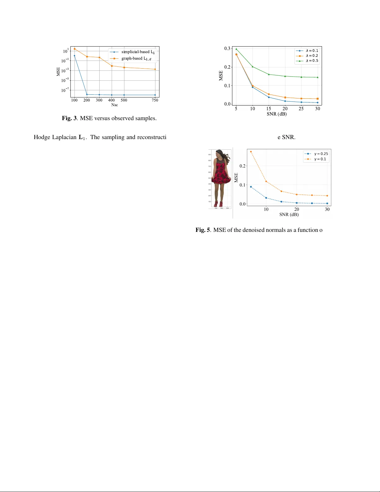
TOPOLOGICAL SIGNAL PR OCESSING FOR 3D POINT CLOUD DA T A T iziana Cattai 1 , Stefania Sar dellitti 2 , Stefania Colonnese 1 , Sergio Barbar ossa 1 1 Dept. of Information Engineering, Electronics and T elecommunications, Sapienza Uni versity of Rome, Italy , 2 Dept. of Engineering and Sciences, Uni versitas Mercatorum, Rome, Italy ABSTRA CT Our goal in this paper is to apply the topological signal pro- cessing (TSP) framework to the analysis of 3D Point Clouds (PCs) represented on simplicial complexes. Building on Dis- crete Exterior Calculus (DEC) theory for v ector fields, we in- troduce higher-order Laplacian operators that enable the pro- cessing of signals over triangular meshes. Unlike traditional approaches, the proposed approach allo ws us to characterize both color attributes, modeled as 3D v ectors on nodes, and ge- ometry , modeled as 3D vectors on the barycenter of each tri- angle. Then, we sho w as TSP tools may ef ficiently be used to sample, reco ver and filter PCs attrib utes treating them as edge signals. Numerical results on synthetic PCs demonstrate ac- curate color reconstruction with robustness to sparse data and geometry refinement in the case of noisy PC coordinates. The proposed approach provides a topology-based representation to characterize the geometry and attributes of PCs. Index T erms — Point Cloud, Discrete Exterior Calculus, T opological Signal Processing. 1. INTR ODUCTION Point Clouds (PCs) are a set of points on a 3D surface and they are ef ficiently used to represent objects and environments in eXtended Reality (XR) applications. Each point of the PC is associated with its 3D coordinates, keeping its shape, to- gether with their attribute, such as color or luminance [1], [2]. A PC typically consists of a very lar ge number of points so that processing operations are often costly and inefficient. T o mitigate these issues, careful sampling strategies need to be designed to select an optimal subset, elaborate a compressed model, and subsequently rebuild the original structure [3]. In this context, the PC geometry plays a fundamental role in the characterization of objects and backgrounds as in, e.g., XR applications. Inaccurate PC coordinates generate uncertain 3D models, and consequently , geometry refinement is a nec- essary task to improv e PC quality and XR usability [4, 5]. This work was supported by the European Union - Next Generation EU under the Italian National Recovery and Resilience Plan (NRRP), Mission 4, Component 2, In vestment 1.3, CUP B53C22004050001, partnership on “T elecommunications of the Future” (PE00000001 - program “REST AR T”). Graph Signal Processing (GSP) tools [6, 7, 8], specifically de- veloped to process signals defined over the nodes of a graph, hav e been applied to model and analyze PC data [9]. Graph- based representations fit well with PC, where each point has a set of features associated [10]. Recently , the T opological Sig- nal Processing (TSP) framework [11] has been dev eloped for processing signals defined on higher order topological spaces than graphs, such as simplicial and cell comple xes [12, 13], to capture higher-order interactions, beyond pairwise relation- ships. In [12], TSP has also been applied to the analysis of planar vector fields, such as, for example, filtering RN A ve- locity vector fields. Contributions. In this paper , we propose a TSP frame- work for PCs, where simplicial complexes are used to model higher-order structures. Based on DEC and Whitney interpo- lation functions, our frame work enables a consistent mapping from vector signals defined on the vertices (color attributes) to scalar signals defined on the edges of a graph. Then, we associate a second order simplicial complex to the graph to exploit triple-wise interactions. The same framework is then extended to represent the PC geometry as vector fields defined on 2 -simplices (triangles). An example is gi ven by the vectors associated to the normal of each triangle. This enables the analysis and refinement of noisy surface models. The main advantage of this approach is its ability to handle both miss- ing attrib utes, such as color information, which may be absent due to compression or acquisition gaps, and uncertainties in the PC geometry , where noisy coordinates af fect the surface normals. The contributions of this paper can be summarized as follo ws: 1) we introduce an algorithmic generalization of the TSP framew ork to 3D PC data processing, modeling the PC as a simplicial complex able to capture higher -order topo- logical relationships among data; 2) we define higher-order Laplacian operators, through DEC and Whitney interpolation functions, that enable the mapping from vector signals on the vertices to scalar signals on the edges, as well as the represen- tation of vector fields on simplicial comple xes; 3) we apply the proposed framework to two key problems in PC process- ing: (i) color recov ery from sparse samples and (ii) geometry refinement under noisy point coordinates. W e validate our approach on synthetic and real PCs. 2. FR OM POINT CLOUD T O SIMPLICIAL COMPLEX By definition, a 3D point cloud P is a set of N points V = { v i , i = 1 , . . . , N } , embedded in a 3D space and carry- ing both geometry and feature information [2]. The positions of the points are determined by the vectors p i = [ x i , y i , z i ] T , i = 1 , . . . , N . Feature vectors are typically attached to each point to encode various attributes of the observed data. A typ- ical example is the color vector ( R , G, B ) . V arious methods hav e been de veloped for generating triangular meshes out of the point cloud [14]. W e build a triangular surface mesh M , applying a well-centered Delaunay triangulation [15], [16]. Each triangle may have associated a feature vector , like, e.g., its normal vector ( n x , n y , n z ) . W e denote with N , E and T the sets of nodes, edges and triangles, respectiv ely , induced by the triangular mesh. The cardinalities of these sets are de- noted as |V | = N , |E | = E and |T | = T . Next, we introduce the concept of geometric simplicial complex (GSC), of which a triangular surface mesh is a typical example. Geometric Simplicial Complexes. Let us define a set of points v i in R d as af finely independent if it is not contained in a hyperplane. An affinely independent set in R d contains at most d + 1 points. A k -simplex σ k is the conv ex hull of k + 1 af finely independent points σ k = ( v 0 , . . . , v k ) . Thus, a point is a 0 -simple x σ 0 , a line segment is a 1 -simplex σ 1 , a triangle is a 2 -simplex σ 2 , and so on. A face of the k -simplex { v i 0 , . . . , v i k } is a ( k − 1) -simple x of the form { v i 0 , . . . , v i j − 1 , v i j − 1 , . . . , v i k } , for some 0 ≤ j ≤ k . A geometric simplicial complex X in R d is a collection of sim- plices in R d such that i) ev ery face of a simplex of X is in X and ii) the intersection of any two simplices of X is either a face of each of them, or it is empty [17]. W e denote by σ k i the simplex i of order k . A ( k − 1) -face σ k − 1 j of a k -simplex σ k i is called a boundary element of σ k i . W e use the notation σ k − 1 j ≺ b σ k i to indicate that σ k − 1 j is a simplex bounding σ k i . A ( k − 1) -simple x σ k − 1 i is incident to a k -simplex σ k j if σ k − 1 i ≺ b σ k j . T wo simplices of order k are lo wer inci- dent if they share a common simplex of order ( k − 1) , or upper incident if the y are faces of a common simplex of or - der k + 1 . The structure of the comple x X is described by the incidences matrices B k with k = 1 , . . . , K , describing which k -simplices are incident to which ( k − 1) -cells, and accounting for simplex orientation. These boundary matrices are defined as [11]: B k ( i, j ) =    1 , if σ k − 1 i ≺ b σ k j and σ k − 1 i ∼ σ k j − 1 , if σ k − 1 i ≺ b σ k j and σ k − 1 i ≁ σ k j 0 , if σ k − 1 i ≺ b σ k j (1) where we use the notation σ k − 1 i ∼ σ k j ( σ k − 1 i ≁ σ k j ) to indi- cate that the orientation of σ k − 1 i is coherent with that of σ k j . Giv en a simplicial complex we can define the signals s 0 : V → R N , s 1 : E → R E and s 2 : T → R T on the sim- 0.5 0.0 0.5 X 0.5 0.0 0.5 Y 0.5 0.0 0.5 Z Fig. 1 . Example of geometric simplicial complex. plicial complex as the signals observed ov er the nodes, edges and triangles, respecti vely . A geometric simplicial complex is a triangular mesh, as it encodes geometry through vertices, edges, and triangular faces. An e xample of a GSC is illus- trated in Fig. 1 where we show a color map on a spheroidal PC, with normal vectors associated to each triangle and colors associated to each simplex. 3. TOPOLOGICAL SIGNALS O VER POINT CLOUDS Giv en a PC, the discrete vector field { v ( p i ) } N − 1 i =0 is a map from the point position p i of X to R 3 . The vectors v ( p i ) ∈ R 3 , i = 0 , · · · N − 1 can be processed applying topological signal processing [11] and discrete e xterior calculus [18]. W e first project each node v ector v ( p i ) on all the edges ha ving node i as an endpoint. More specifically , denoting by m 1 , m 2 the endpoints of edge m , we build the scalar signal on edge m , for m = 1 , . . . , E , as s 1 m = 1 2  ( p m 2 − p m 1 ) ⊤ v ( p m 1 ) + ( p m 2 − p m 1 ) ⊤ v ( p m 2 )  . (2) Thus, we obtain a scalar field defined over the edges of the simplicial complex. Ne xt, we use Whitney interpolation [19] to compute the vector associated to the barycenter of each triangle, as follo ws. Let us define by v ( p ; σ 2 ) = T σ v ( p ) the vector at position p tangential to the triangle σ 2 , where T σ = I − n σ n T σ with n σ the normal to the triangular face. According to Whitney interpolation, we reconstruct from the edge signal in (2) the field v ( p ; σ 2 ) as v ( p ; σ 2 ) = E X m =1 s 1 m ·  φ (2) m 1 ( p ) ∇ φ (2) m 2 ( p ) − φ (2) m 2 ( p ) ∇ φ (2) m 1 ( p )  , p ⊂ σ 2 (3) where φ (2) i ( p ) is an affine piece wise function, belonging to the class of Whitney interpolation functions and σ 2 ∈ T i , with T i the subset of triangles to which the i-verte x belongs to. The Whitney interpolation functions of order k are sup- ported o ver k -simplices [18]. The function φ (2) i ( p ) is sup- ported on the 2 -simplices having one verte x in p i , i.e. for each p in T i . On each of the 2 -simplices, φ (2) i ( p ) takes v alue 1 at p i and decreases linearly to zero at the other vertices. The final step consists in e valuating the vector field o ver the vertices of the original point cloud. T o do that, we first deriv e all the vectors on the barycenters p σ of each trian- gle, setting p = p σ in (3). In this manner, the tangential vector field computed o ver all the barycenters is v i ( σ 2 ) = v ( p ; σ 2 ) | p = p σ 2 . Giv en the collection of tangential compo- nents v i ( σ 2 ) , σ 2 ∈ T i , the discrete vector field v i at the i -th graph verte x is reconstructed in closed-form as [20] [21]: v i =   X σ 2 ∈T i T ⊤ σ T σ   − 1 X σ 2 ∈T i T ⊤ σ v i ( σ 2 ) (4) provided that the signal v i is not perpendicular to all the inci- dent faces, i.e. ∃ σ 2 ∈ T i | v i ⊥ σ 2 . Finally , the adoption of the Whitney interpolation func- tion to reconstruct the vector field ov er the 2-simplices allo ws to endo w the abov e defined notion of incidence between sim- plices with a geometric metric. This leads to the definition of the first-order discrete Laplacian L 1 , weighted with the metric matrices M p as [22] L 1 = M 1 B T 1 M − 1 0 B 1 M 1 + B 2 M 2 B T 2 (5) where the weighting matrices M 0 , M 1 and M 2 , depend on the forms used for vector field interpolation [23]. Using the Whit- ney interpolation functions on k -simplices, the metric matri- ces M k define Whitney inner products between signals, with entries giv en by | M k | ij = ⟨ φ ( k ) i , φ ( k ) j ⟩ , k = 0 , 1 , 2 . (6) The weighted first-order Laplacian in (5) is composed of two terms: the first term L 1 ,d = M 1 B T 1 M − 1 0 B 1 M 1 describes the lo wer adjacencies between edges, while the second term L 1 ,u = B 2 M 2 B T 2 described the upper adjacencies of edges as boundaries of triangles. Then, L 1 provides an algebraic representation of the triangular mesh enabling the use of the topological signal processing frame work [11] for processing signals observ ed o ver the edges of a GSC. Specifically , de- noting with U = { u m } E m =1 the eigen vectors of the first order Laplacian matrix L 1 , the Simplicial Fourier T ransform (SFT) ˆ s 1 of the edge signal s 1 is defined as ˆ s 1 = U T s 1 . This trans- form provides the spectral representation of the edge signals as s 1 = U T ˆ s 1 . 4. POINT CLOUD COLOR RECO VERY Let us now consider the vector field of the colors observ ed ov er a PC, i.e. a map from the point position p i of X to [0 , 1] 3 . In the previous section, we showed how using (3) we can re- cov er the point cloud color , represented as a discrete vector field, from scalar signals on the edges s 1 m , m = 1 , . . . , E . Fig. 2 . (a) T oroidal PC and (b) associated discrete color vector field. Howe ver , in man y practical applications, color attrib utes may be missing for some points due to sensor errors, or intention- ally subsampled during compression to reduce the bit rate. In such cases, the scalar signal s 1 m is unav ailable on some edges. W e address the problem of recov ering s 1 m , ∀ m , from its val- ues on a subset S of observed edges, assuming |S | < E . T o identify the optimal sampling set we use the greedy MaxDet strategy in [24]. Let us e xpress the sampled edge signal in vector form as: y 1 = D S s 1 (7) where s 1 =  s 1 1 , · · · s 1 E  T and D S is an edge-selection diag- onal matrix whose m -th diagonal entry is 1 if m ∈ S , and 0 otherwise. The conditions for reco vering the edge signal s 1 from its edge samples in S are giv en in [11], [24] in terms of its SFT [11]. Let us assume that the edge signal s 1 is K -bandlimited, i.e. it can be represented over K eigenv ectors U K = { u i } i ∈K of frequency inde xes i ∈ K , i.e. s 1 = U K ˆ s 1 K . W ith these positions, the edge signal s 1 is recovered from N sc = |S | samples with N sc > K [24] as follo ws: s 1 =  I −  I − D S  U K U T K  − 1 y 1 . (8) W e assess the reconstruction performance of the proposed approach on a toroidal PC, with N = 600 points of coordi- nates bounded in [0 , x max ] × [0 , y max ] × [0 , z max ] . The as- sociated triangular mesh was built via a standard parametric tessellation, leading to E = 1800 edges and T = 1200 trian- gles. The point cloud color [ R i , G i , B i ] at node i is assigned as R i = x i x max , G i = y i y max , B i = z i z max . This setup en- sured a smooth color distribution over the point cloud that we used as the ground truth signal. Specifically , the point cloud color attrib ute is represented by the discrete vector field v i = [ R i , G i , B i ] T , i = 0 , · · · N − 1 . Figure 2 represents the colored point cloud and the qui ver plot of the discrete vec- tor field v i , i = 0 , · · · N − 1 . Then, using (8) we reco ver the edge signal s 1 from its values collected o ver a subset S of edges with N sc < E . W e compared two reconstruction strate- gies: (i) the graph-based reconstruction relying only on the edge Laplacian L 1 ,d (without considering triangles), and (ii) the proposed simplicial-comple x reconstruction using the full 100 200 300 400 500 750 Nsc 1 0 7 1 0 5 1 0 3 1 0 1 1 0 1 MSE s i m p l i c i a l - b a s e d L 1 g r a p h - b a s e d L 1 , d Fig. 3 . MSE versus observ ed samples. Hodge Laplacian L 1 . The sampling and reconstruction pro- cess was carried out by v arying the number of sampled nodes N sc from 100 to 750 and recovering the edge signal ˆ s 1 . In Fig. 3, we report the mean square error MSE = ∥ ˆ s 1 − s 1 ∥ be- tween the reconstructed and original signals. The results sho w how the use of simplicial complexes significantly improves the accurac y of the reconstruction with respect to graph-based representation. This confirms that incorporating higher-order topological information provides a richer basis for signal rep- resentation, enabling a more accurate recovery of the under- lying edge signals from sparse samples. 5. POINT CLOUD GEOMETR Y REFINEMENT When capturing the PC from sensors like LiD AR or lasers, the coordinates of the points may be af fected by errors. This geo- metric perturbation translates into noise on the normals of the planes defined by the mesh triangles. T o deal with this kind of perturbation, we treat the vector associated with the normals as a signal defined over the triangles of the simplicial com- plex. The problem can then be cast as a geometry noise fil- tering, in volving the weighted the second-order Hodge Lapla- cian matrix [25] L 2 = M 2 B T 2 M − 1 1 B 2 M 2 . (9) Specifically , we formulate the geometry refinement as the fol- lowing optimization problem: min s 2 ∈ R T ∥ s 2 − x 2 ∥ 2 + λ s 2 ⊤ L 2 s 2 + γ ∥ s 2 ∥ 1 (10) where x 2 are the noisy signals giv en by the normals to the triangular f aces, while s 2 is the filtered estimate signal. Our goal is to minimize a weighted sum of data fitting error, sig- nal smoothness, and sparsity . Specifically , the first term of the objecti ve function is the data fitting error , the second term represents the smoothness of the signal o ver the second-order Hodge Laplacian L 2 , while the third term is introduced to control the signal sparsity . The coef ficients γ and λ are tuned to control the trade-off between the objective function terms. W e tested the proposed algorithm on the same PC described in the previous section to denoise triangular signals on simpli- cial complexes, i.e. the normals to the triangles. Specifically , 5 10 15 20 25 30 SNR (dB) 0.0 0.1 0.2 0.3 MSE = 0 . 1 = 0 . 2 = 0 . 5 Fig. 4 . MSE of the denoised normals with respect to the noiseless case, as a function of the SNR. Fig. 5 . MSE of the denoised normals as a function of the SNR for Red and Black PC varying γ with a fixed λ = 0 . 1 . we add Gaussian noise to the normals, which corresponds to perturbing the geometry of the PC. In Fig. 4, we show the MSE of the denoised normals with respect to the noiseless case, as a function of the signal-to-noise ratio (SNR). The re- sults are obtained by fixing γ = 0 . 1 and v arying λ in the set { 0 . 1 , 0 . 2 , 0 . 5 } , leading to three dif ferent curves. As ex- pected, the curves sho w an improv ement in performance with increasing SNR. Furthermore, a smaller λ leads to a lower MSE, as the data fitting term pre v ails in the optimization. W e also test our method on a real PC (Red and Black) [26] and we show the ability of the proposed approach to refine geometry in presence of additiv e noise in Fig. 5. 6. CONCLUSIONS In this paper we employed the topological signal processing framew ork for processing a PC, modeled as a vector field de- fined on a set of points whose coordinates may be af fected by errors. W e showed that le veraging the higher order structure improv es color reco very over graph-based methods, and that geometry refinement can be effecti vely performed. Of course, there is a lot to be done to extend our approach to cases where the filtering operator and the geometry refinement can be im- plemented jointly . A v ery interesting aspect to be inv estigated is the use of space-varying filtering operator that adapts the support of its kernel to the curv ature of the point cloud. 7. REFERENCES [1] D. Graziosi, O. Nakagami, S. Kuma, A. Zaghetto, T . Suzuki, and A. T abatabai, “ An ov erview of ongo- ing point cloud compression standardization activities: V ideo-based (V-PCC) and geometry-based (G-PCC), ” APSIP A T rans. on Signal and Inform. Pr ocess. , vol. 9, pp. e13, 2020. [2] C. Cao, M. Preda, and T . Zaharia, “3D point cloud com- pression: A survey , ” in Pr oc. of the 24th Inter . Conf. on 3D W eb T ec hnology , 2019, pp. 1–9. [3] S. N. Sridhara, E. Pav ez, A. Jaya want, A. Ortega, R. W atanabe, and K. Nonaka, “Graph-based scalable sampling of 3D point cloud attrib utes, ” arXiv pr eprint arXiv:2410.01027 , 2024. [4] E. Mattei and A. Castrodad, “Point cloud denoising via moving RPCA, ” in Computer Graphics F orum . Wile y Online Library , 2017, vol. 36, pp. 123–137. [5] M. A. Irfan and E. Magli, “Joint geometry and color point cloud denoising based on graph wa velets, ” IEEE Access , vol. 9, pp. 21149–21166, 2021. [6] D. I. Shuman, S. K. Narang, P . Frossard, A. Ortega, and P . V andergheynst, “The emerging field of signal processing on graphs: Extending high-dimensional data analysis to networks and other irregular domains, ” IEEE Signal Pr ocess. Mag. , v ol. 30, no. 3, pp. 83–98, 2013. [7] A. Anis, A. Gadde, and A. Ortega, “T ow ards a sam- pling theorem for signals on arbitrary graphs, ” in 2014 ICASSP . IEEE, 2014, pp. 3864–3868. [8] S. Chen, R. V arma, A Sandryhaila, and J. K ov a ˇ cevi ´ c, “Discrete signal processing on graphs: Sampling the- ory , ” IEEE T ransactions on Signal Pr ocessing , vol. 63, no. 24, pp. 6510–6523, 2015. [9] W . Hu, J. Pang, X. Liu, D. T ian, C.-W . Lin, and A. V etro, “Graph signal processing for geometric data and be- yond: Theory and applications, ” IEEE T rans. on Multi- media , vol. 24, pp. 3961–3977, 2021. [10] M. Zhao, L. Ma, X. Jia, D.-M. Y an, and T . Huang, “GraphReg: Dynamical point cloud registration with geometry-aware graph signal processing, ” IEEE T rans. on Image Pr ocess. , vol. 31, pp. 7449–7464, 2022. [11] S. Barbarossa and S. Sardellitti, “T opological signal processing over simplicial complex es, ” IEEE T rans. on Signal Pr ocess. , vol. 68, pp. 2992–3007, 2020. [12] S. Sardellitti and S. Barbarossa, “T opological signal processing ov er generalized cell comple xes, ” IEEE T rans. Signal Process. , 2024. [13] M. T . Schaub, Y . Zhu, J.-B. Seby , T . M. Roddenberry , and S. Segarra, “Signal processing on higher-order net- works: Li vin’on the edge... and beyond, ” Signal Pr o- cess. , vol. 187, pp. 108149, 2021. [14] L. Linsen, P oint cloud r epresentation , Uni v ., Fak. f ¨ ur Informatik, Bibliothek T echnical Report, 2001. [15] D.-T . Lee and B. J. Schachter , “T w o algorithms for con- structing a Delaunay triangulation, ” Inter . Jour . of Com- puter & Information Sciences , vol. 9, no. 3, pp. 219– 242, 1980. [16] L. Chen and J.-C. Xu, “Optimal Delaunay triangu- lations, ” Journal of Computational Mathematics , pp. 299–308, 2004. [17] A.N. Hirani, Discr ete exterior calculus , California In- stitute of T echnology , 2003. [18] M. Desbrun, A. N. Hirani, M. Leok, and J. E. Mars- den, “Discrete exterior calculus, ” arXiv preprint math/0508341 , 2005. [19] J. Dodziuk, “Finite-difference approach to the hodge theory of harmonic forms, ” American Journal of Math- ematics , vol. 98, no. 1, pp. 79–104, 1976. [20] C. R. Rao and S. K. Mitra, “Generalized in verse of a ma- trix and its applications, ” in Proc. of the Sixth Berkele y Symp. on Mathem. Statis. and Pr ob ., . Uni v . of California Press, 1972, vol. 6, pp. 601–621. [21] S. K. Mitra and C. R. Rao, “Projections under semi- norms and generalized Moore Penrose in verses, ” Linear Algebra and its Applications , v ol. 9, pp. 155–167, 1974. [22] M. Fisher, P . Schr ¨ oder , M. Desbrun, and H. Hoppe, “De- sign of tangent vector fields, ” ACM T rans. on Graphics (TOG) , v ol. 26, no. 3, pp. 56–es, 2007. [23] N. Bell and A. N. Hirani, “Pydec: software and al- gorithms for discretization of exterior calculus, ” A CM T rans. on Mathematical Softwar e (TOMS) , vol. 39, no. 1, pp. 1–41, 2012. [24] M. Tsitsvero, S. Barbarossa, and P . Di Lorenzo, “Signals on graphs: Uncertainty principle and sampling, ” IEEE T rans. on Signal Pr ocessing , vol. 64, no. 18, pp. 4845– 4860, 2016. [25] A. N. Hirani, K. Kalyanaraman, H. W ang, and S. W atts, “Cohomologous harmonic cochains, ” arXiv preprint arXiv:1012.2835v2 , 2010. [26] E. d’Eon, B. Harrison, T . Myers, and P . A. Chou, “8i vox elized full bodies-a vox elized point cloud dataset, ” ISO/IEC JTC1/SC29 J oint WG11/WG1 (MPEG/JPEG) input document WG11M40059/WG1M74006 , v ol. 7, no. 8, pp. 11, 2017.