A mixed Hinfty-Passivity approach for Leveraging District Heating Systems as Frequency Ancillary Service in Electric Power Systems

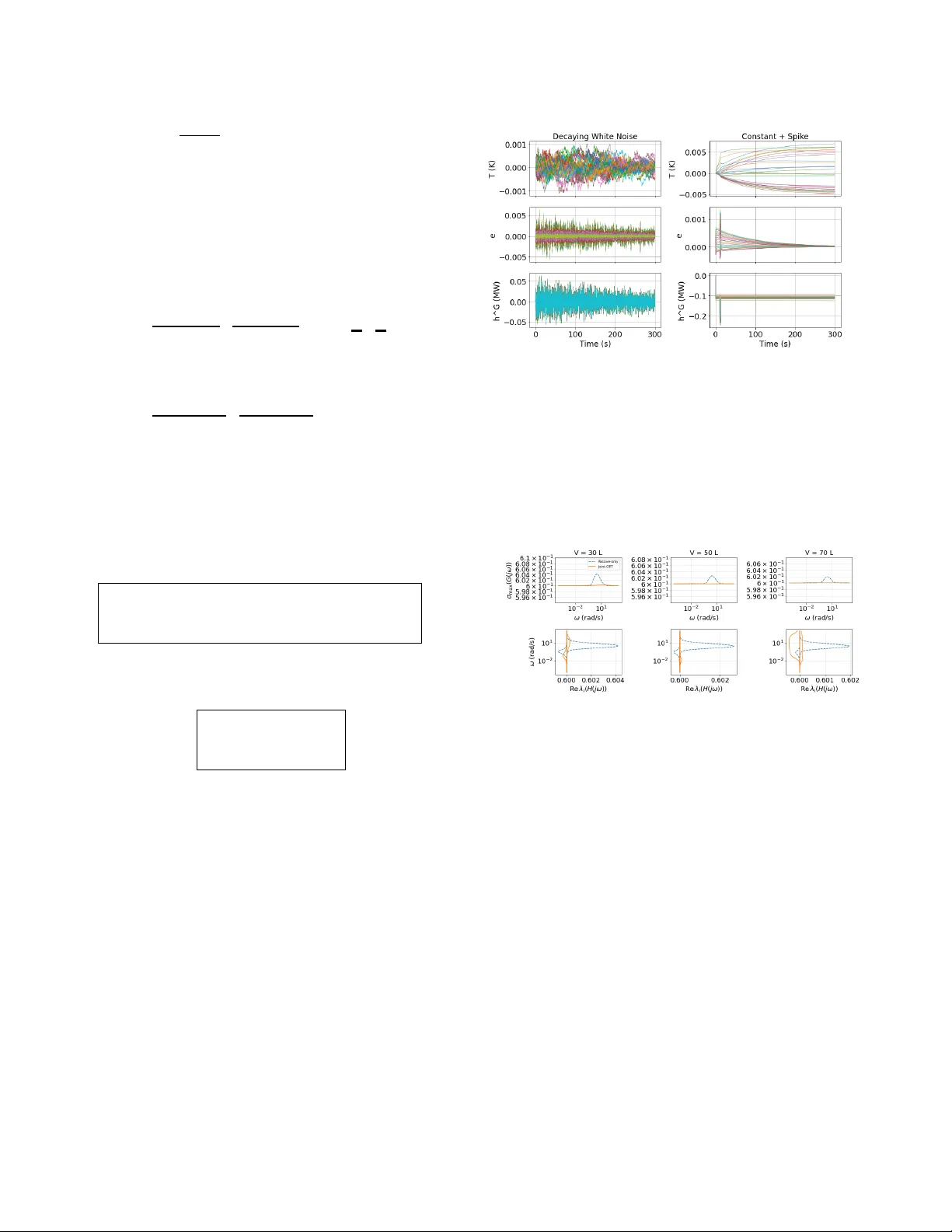
A mix ed H ∞ –P assi vity approach for Le v eraging District Heating Systems as Frequenc y Ancillary Service in Electric Po wer Systems Xinyi Y i and Ioannis Lestas Abstract —This paper introduces a mixed H ∞ –passivity frame- work that enables district heating systems (DHSs) with heat pumps to support electric-grid frequency regulation. The analysis in the paper illustrates how the DHS regulator influences coupled electro–thermal frequency dynamics and pro vides LMI condi- tions for efficient controller design. A disturbance-independent temperature regulator is also presented that ensures stability and rob ustness against heat-demand uncertainty . Simulations demon- strate improved frequency control dynamics in the electrical power grid, while maintaining good thermal performance in the DHS. I . I N T R O D U C T I O N As decarbonization accelerates, electrified heating is becom- ing central to low-carbon energy systems. Heat pumps (HPs) enable ef ficient electricity-to-heat con version and significantly tighten the coupling between electric power systems (EPSs) and district heating systems (DHSs). Large-scale initiativ es including the EU Heat Pump Accelerator [1] and China’ s National Action Plan [2] highlight the rapid growth of HP deployment. At the same time, the expansion of lar ge data cen- ters increases the need for fast and reliable ancillary services, intensifying the demand for flexible resources. Leveraging their inherent thermal storage capacity , DHSs present strong potential to contribute to EPS frequency support. Frequency regulation in EPSs is hierarchical: primary con- trol acts within seconds, secondary restores nominal fre- quency within minutes, and tertiary optimizes long-term oper- ation. The thermal inertia of DHSs fits the secondary-control time scale. DHSs typically use optimal setpoint scheduling and tracking, where energy-sharing optimization yields cost- efficient setpoints and controllers follow them. Y et uncertain thermal demand causes setpoint deviations. Our prior work [3] proposed an LQR temperature regulator achieving optimal power sharing within a heating system without having a prior knowledge of the disturbances. The integration of such in- volv ed control schemes within a po wer system, while ensuring good performance in the combined electrothermal network is though a non-tri vial problem. Recent studies have examined coordinated frequency– tem- perature control in combined heat and power (CHP) systems. [4] introduced a Port-Hamiltonian framework, b ut it depends on disturbance-based temperature setpoints that are hard to X. Yi and I. Lestas are with the Department of Engineering, University of Cambridge, Trumpington Street, Cambridge, CB2 1PZ, United Kingdom. Emails: @cam.ac.uk . Accepted by 2026 IEEE Po wer & Energy Society General Meeting specify under renewable variability and complex demand pat- terns. [5] proposed a distributed primary-frequency controller with a disturbance-independent av erage-temperature based regulator , while [6] used rob ust MPC with data-dri ven distur- bance forecasts to provide frequency support under building- scale thermal constraints. Howe ver , prior work does not assess how the the DHS temperature-regulator design affects closed- loop electro–thermal dynamic interactions and performance when HPs contrib ute to frequenc y regulation. This study addresses this gap using a mix ed H ∞ –passivity framework that links DHS re gulator structure to CHP frequency control performance. In particular , a mix ed H ∞ –passivity method is proposed that ensures stability and enhances performance, while achieving optimal energy sharing in the DHS. Furthermore, it yields tractable LMI conditions for the DHS temperature controller design. The key contributions of this paper are: 1) A DHS regulator is proposed that con ver ges to the optimal electro– thermal operating point under uncertain demand; 2) A mixed H ∞ –passivity frame work is formulated linking DHS regulator structure to CHP frequency-control dynamic behaviour , en- abling more efficient frequenc y support; 3) Analytical conv er- gence guarantees are pro vided for the CHP system considered. The paper is structured as follows. Section II formulates the DHS–EPS model, Section III dev elops and analyzes the con- trol scheme, and Section IV presents simulation case studies. I I . S Y S T E M M O D E L F O R M U L A T I O N In the paper , bold symbols denote stacked v ectors, and when clear from context, matrices. Non-bold symbols represent scalar quantities. All proofs are provided in the Appendix to preserve technical clarity and comply with page limits. A. Heat pump Let H e denote the set of b uses in the EPS where HPs are connected, H h the set of DHS edges associated with HPs, and H H P the set of HP units. For frequency regulation, each HP operates near an equilibrium point with approximately constant coefficient of performance (CoP), so that its elec- tric power consumption p H k , heat output h P k , bus frequency deviation ω i and DHS signal S ig H satisfy [4], [5], [7] : h P j k = C oP k · p H i k , j k ∈ H h , i k ∈ H e , (1a) p H k = γ E k ω k + γ H k S ig H , k ∈ H H P , (1b) where γ E k and γ H k denote the electrical and thermal operation coefficients of HP k , respectively . B. Electric power system 1) F requency dynamic model of electric buses: T wo types of buses are considered: i ∈ E DG , which connect only to distributed generators (DGs), and i ∈ E H P , which host both DGs and heat pumps (HPs), and E = E DG ∪ E H P . Let P i denote the net acti ve po wer flo wing out of b us i . The frequency deviation, damping coef ficient, controllable generation, control input, electrical disturbance, and inertia at bus i are denoted by ω i , D i , P G i , u i , P L i , and M i , respecti vely . Here, ω i , u i , P L i , P i , and P G i represent deviations from their nominal steady- state values. T o capture the lag in the response of generation, each controllable unit is modeled with a first-order system: T g ,i ˙ P G i = − P G i + u i , i ∈ E , (2) where T g ,i > 0 is the effecti ve turbine–go vernor time constant. The bus frequency dynamics are then gi ven by M i ˙ ω i = − D i ω i − P i + P G i , i ∈ E DG , (3a) M i ˙ ω i = − D i ω i − P i + P G i − p H i , i ∈ E H P , (3b) where p H i is the acti ve po wer consumed by the HP at bus i , computed according to (1b). The network po wer flo w and angle dynamics are: P i = X j | B ij | V i V j sin( θ i − θ j ) − P L i , i ∈ E , ˙ x θ = R I ω , (4) where x θ is the phase-angle deviation vector e xcluding the reference bus r , ω denotes frequenc y vector , and R I = [ I n E − 1 , − 1 n E − 1 ] . n E denotes the number of electric buses, while I x and 1 x represent the identity matrix and the all-ones vector of dimension x , respectiv ely . Assumption 1. F or any ¯ P L and ¯ p H , the EPS (2-4) ad- mits an equilibrium ( x ∗ θ , θ ∗ , ω ∗ , P G ∗ , P ∗ , u ∗ ) , wher e ω ∗ = ω com 1 n E and ω com is the synchr onized EPS frequency . 2) Secondary fr equency contr ol: The objectiv e of sec- ondary frequency control is to restore the frequency to its nominal value, achiev ed via A GC integral control at bus r : ˙ g = − ω r , u i = − K P i ω i + δ ir K I g , i ∈ E , (5) where K P i > 0 are droop gains, and K I > 0 is the A GC gain. If i = r , δ ir = 1 , otherwise, δ ir = 0 . Lemma 1. Under Assumption 1 , for any constant disturbances ¯ P L and ¯ p H , the EPS model with the A GC contr oller (2) - (5) admits a unique equilibrium ( x ∗ θ , θ ∗ , u ∗ , ω ∗ , P G ∗ , P ∗ , g ∗ ) . At this equilibrium, ω ∗ = 0 . Assumption 2. F or all i ∈ E the damping coefficients satisfy D i ≥ D min > 0 . The closed–loop generation dynamics (2,5) at each b us are of first order with time constant T g ,i > 0 . The transfer function from − ω i to the gener ated power P G i is G i ( s ) := D i + K P i T g ,i s + 1 + δ ir K I s ( T g ,i s + 1) , (6) wher e the last term is pr esent only at the refer ence bus r . Each G i ( s ) is strictly positive r eal, i.e., there exists ρ i > 0 such that ℜ G i ( j ω ) ≥ ρ i for all ω ∈ R . 1 Lemma 2. Under Assumptions 1-2 , consider the EPS model with the AGC contr oller (2) - (5) . W ith the input u 1 := − p H , and the output y 1 := ω H P , the EPS is strictly passive from u 1 to y 1 : ther e e xist a stora ge function V e and a constant ρ e > 0 such that along all trajectories with the squared Euclidean norm ∥ y 1 ∥ 2 := y ⊤ 1 y 1 : ˙ V e ≤ y ⊤ 1 u 1 − ρ e ∥ y 1 ∥ 2 . (7) C. District heating system 1) T emperatur e dynamics: W e model the DHS temperature dynamics following [5]. Let H E denote the set of edges (heat exchangers and pipelines) and H N the set of nodes (storage tanks). The edge and node dynamics are given as follows: ρC p V E j ˙ T E j = ρC p q E j ( T N k − T E j ) + h G j + h P j − h L j , j ∈ H E , k ∈ H N , (8a) ρC p V N k ˙ T N k = X j ∈T k ρC p q E j ( T E j − T N k ) , k ∈ H N , (8b) where T E j and T N k denote the outlet temperatures of edge j and node k , respecti vely . h P j , h G j , and h L j represent the heat contributions from the HP , the con ventional heat source, and the thermal load at edge j . The parameters V E j and V N k are the volumes of edges and nodes, q E j is the mass flo w along edge j , and C p and ρ denote the specific heat capacity and density of water . The HP heat injection h P j corresponds to h P j k in (1a). If edge j hosts an HP , then h G j = h L j = 0 ; for a conv entional heat source, h P j = h L j = 0 ; and for a load, h G j = h P j = 0 with fixed h L j . Equations (8a)–(8b) can be compactly expressed in matrix form using the Kirchhof f matrix A h [5]. V      ˙ T G ˙ T H P ˙ T L ˙ T N      = − A h     T G T H P T L T N     +    h G 0 0 0    +    0 h P 0 0    +    0 0 − h L 0    , (9a) ˙ T = − AT + B 1 h G + B 2 h P + w h , (9b) where h G , h P , and h L denote the non-pump heat source gen- eration, HP generation, and load vectors, respectively . W e define A = A h V , B 1 = I V    I 0 0 0    , B 2 = I V    0 I 0 0    , w h = I V    0 0 − h L 0    . 2) Ener gy-sharing steady-state objectives: The steady-state economic dispatch for DHSs under given ¯ h P and ¯ w h is modeled as two optimization problems. E1: min h G ∈ R , T ∈ R Φ 1 = 1 2 h G ⊤ F G h G , (10a) s.t. AT = B 1 h G + B 2 ¯ h P + ¯ w h , (10b) 1 Note that higher order generation dynamics that satisfy this property can also be considered. where Φ 1 denotes the non-pump sources’ heat generation cost, with F G = diag { f G i } , where f G i > 0 is the cost coefficient of source i . The temperature deviation cost is minimized in E2 , formulated as: E2: min z ∈ R , T ∈ R Φ 2 = 1 2 T ⊤ F D T , (11a) s.t. T = A † ( B 1 h G ∗ + B 2 ¯ h P + ¯ w h ) + α 1 , (11b) where A † denotes the Moore–Penrose pseudoin verse of A , and F D = diag { F D i } , with F D i > 0 , is the temperature deviation penalty coefficient associated with node or edge i . Lemma 3. (Optimality condition for E1 and E2 [3]) If the DHS (9b) achie ves equilibrium at T ∗ and h G ∗ , and satisfies F M h G ∗ = 0 and 1 ⊤ F D T ∗ = 0 , then it uniquely 2 solves the optimization pr oblems E1 and E2 , wher e F M is defined by the following matrix:    F G (1 , 1) − F G (2 , 2) 0 · · · 0 0 F G (2 , 2) − F G (3 , 3) · · · 0 . . . . . . . . . . . . . . .    . (12) The error is defined as: e = C T + D h G =  e G S ig H  , S ig H = s T e , . (13) where C =  0 1 ⊤ F D  , D =  F M 0  , and s T =  0 ⊤ 1  3) Augmented DHS: Substituting (1) into (9b): ˙ T = ( − A + B s C ) T + ( B 1 + B s D ) h G + B 2 C oP γ E w H P + w h (14a) = A e T + B e h G + B ω ω H P + w h , (14b) where C oP = diag ( C oP i ) , B ω = B 2 C oP γ E , and B s = B 2 C oP γ H 1 n H P s T . Integrating ˙ ξ = e obtains:  ˙ T ˙ ξ  =  A e 0 C 0  | {z } ≜ A Aug  T ξ  +  B e D  | {z } ≜ B Aug h G +  B ω 0  | {z } ≜ B ( ω ) cl ω H P +  I 0  |{z} ≜ B ( h ) cl w h . (15) W ith x =  T ⊤ ξ ⊤  ⊤ , (15) can be rewritten as: ˙ x = A aug x + B aug h G + B ( ω ) cl ω H P + B ( h ) cl w h . (16) The input is u 2 = ω H P and the output is defined as y 2 = p H : p H = γ E ω H P + γ H S ig H 1 n H P = γ E ω H P + γ H  1 n H P s T C 0  | {z } ≜ S C x − γ H 1 n H P s T D | {z } ≜ S D K x = γ E ω H P + C y ( K ) x . (17) Lemma 4. Consider the augmented DHS dynamics in (15) with the temperatur e re gulator h G = − K T T − K I ξ . The resulting closed- loop temperatur e dynamics are ˙ x = A cl x + B ( ω ) cl ω H P + B ( h ) cl w h , (18) wher e A cl =  A e − B e K T − B e K I C − D K T − D K I  . If A cl is Hurwitz, the closed-loop DHS admits a unique equilibrium. Mor eover , for constant disturbances ¯ ω H P and ¯ w h , lim t →∞ e ( t ) = 0 . 2 Because Φ 1 and Φ 2 are strictly conv ex ( F D ≻ 0 , F G ≻ 0 ) under linear constraints, the optimizer ( T ∗ , h G ∗ ) of E1 – E2 is unique. I I I . PA S S I V I T Y - BA S E D F R E Q U E N C Y A N D T E M P E R A T U R E C O N T R O L The EPS, with input u 1 and output y 1 , and the DHS, with input u 2 and output y 2 , are interconnected in the CHP system through the relations u 1 = − y 2 and u 2 = y 1 . A. Stability and optimality of the CHP system Lemma 5. Under Assumption 1 , the unique CHP equilibrium ( x ∗ θ , θ ∗ , u ∗ , ω ∗ , P G ∗ , P ∗ , g ∗ , h G ∗ , ξ ∗ , T ∗ , e ∗ , h P ∗ , p H ∗ ) satis- fies ω ∗ = 0 and e ∗ = 0 . Furthermore , the equilibrium meets the contr ol objectives of both subsystems: lim t →∞ ω i = 0 for all i ∈ E ( Lemma 1 ); and lim t →∞ T = T ∗ , lim t →∞ h G = h G ∗ ( Lemma 3 ). Theorem 1. Under Assumptions 1-2 , if the closed-loop augmented DHS in (17) – (18) is strictly passive with r espect to the input–output pair ( u 2 = ω H P , y 2 = p H ) , and if A cl is Hurwitz, then the CHP equilibrium defined in Lemma 5 is asymptotically stable. B. Mixed H ∞ /P assivity Controller Design 1) P assivity-based contr oller design: From Theor em 1 , the temperature regulator h G = − K x must satisfy: (i) A cl is Hurwitz; (ii) the closed-loop augmented DHS (17–18) is strictly passive with input ω H P and output p H = C y ( K ) x + γ E ω H P . The system is strictly passiv e and A cl is Hurwitz if there exist P ≻ 0 and ρ > 0 , " A cl ⊤ P + P A cl P B ( ω ) cl − C y ( K ) ⊤ ∗ − ( γ E + γ E ⊤ ) − ρ I # ≺ 0 . (19) T o transform original KYP-based passivity BMI (19) into LMI for optimization, we introduce the variables X := P − 1 ≻ 0 and Y := K X . The KYP-based passivity BMI (19) is equiv alent to " LM I 1 LM I 2 LM I 2 ⊤ −  γ E + γ E ⊤  − ρ I # ≺ 0 , X ≻ 0 , ρ > 0 . (20) where LM I 1 :=  A aug X − B aug Y  +  A aug X − B aug Y  ⊤ and LM I 2 := B ( ω ) cl − X S ⊤ C + Y ⊤ S ⊤ D . Lemma 6. The original DHS (14) is intrinsically low-pass. Let G ( s ) be the closed-loop transfer matrix fr om ω H P to p H for the augmented DHS (17) – (18) . It satisfies lim ω → 0 G ( j ω ) = γ E . In the low-frequency regime, the DHS behav es as a slo wly varying thermal-storage system, so G ( j ω ) provides a useful “vir - tual damping” effect to the EPS. As disturbances reach the DHS time scale (about 50 – 300 s or 0 . 003 – 0 . 02 Hz), pipeline inertia and transport delay introduce significant phase lag, exciting internal diffusi ve modes rather than attenuating them. Consequently , G ( j ω ) loses its damping role and becomes a mid-frequency cross-coupling amplifier , returning stored thermal energy toward the EPS interface and reducing robustness. At high frequencies, the DHS is strongly diffusi ve, and G ( j ω ) acts mainly as a parasitic cross-coupling path; any non-negligible gain in this range increases the transmission of high-frequency disturbances across the EPS–DHS boundary . This motiv ates a loop-shaping design that suppresses the mid- and high-frequency magnitude of G ( j ω ) while preserving its lo w- frequency behavior . Such shaping pre vents excitation of DHS thermal modes and limits unwanted cross-coupling without sacrificing the beneficial low-frequenc y virtual damping. The goal is therefore to attenuate the mid- and high-frequency components of the chan- nel ω H P 7→ p H while keeping its low-frequency characteristics essentially unchanged. Reducing ∥ G ( j ω ) ∥ in this non-damping band mitigates cross-coupling, improves disturbance rejection, and enhances robustness of the DHS–EPS interaction. 2) H ∞ fr equency–shaping filter: W e introduce a high-pass weighting filter for loop–shaping and impose an H ∞ performance constraint on the weighted output. The high-pass weight is chosen as W HP ( s ) = α + s/ω h 1+ s/ω h , 0 < α ≪ 1 , where ω h > 0 is the cutof f frequency of the first-order low-pass factor 1 / (1 + s/ω h ) . A state- space realization of the filter is ˙ x ω = − ω h x ω + ω h p H , z = (1 + α ) p H − x ω , where x ω ∈ R n H P stores the lo w-frequency component of p H , while z represents the weighted high-frequency component to be minimized under the H ∞ criterion. The small constant α slightly elev ates the lo w-frequency gain for numerical rob ustness and does not affect the cutoff frequency ω h . Define the augmented weighted state x lp =  x ⊤ x ω ⊤  ⊤ , ( ω H P → z ) admits the state-space form: ˙ x lp =  A cl ( K ) 0 ω h C y ( K ) − ω h I n H P  | {z } A lp ( K ) x lp + " B ( ω ) cl 0 # | {z } B lp ω H P +  B ( h ) cl 0  w h , (21a) z =  (1 + α ) C y ( K ) − I n H P  | {z } C lp ( K ) x lp , D lp = 0 . (21b) The Bounded Real Lemma (BRL) provides the suf ficient condition for ∥G ω H P → z ∥ ∞ < γ ∞ as the existence of P lp ≻ 0 such that    A lp ( K ) ⊤ P lp + P lp A lp ( K ) P lp B lp C lp ( K ) ⊤ B ⊤ lp P lp − γ 2 ∞ I 0 C lp ( K ) 0 − I n H P    ≺ 0 . (22) The BRL-based low-pass performance BMI (22) is equi valent to   Ψ 11 B lp Ψ 13 B ⊤ lp − γ 2 ∞ I 0 Ψ 31 0 − I n H P   ≺ 0 , X ≻ 0 , q ω > 0 , (23) where Ψ 11 , Ψ 13 , and Ψ 31 := Ψ ⊤ 13 are defined in Appendix. Combining the KYP-based passi vity LMI (20) and the BRL-based LMI (23), the controller design can be formulated as: min X , Y ,q ω ,ρ,γ ∞ γ 2 ∞ s.t. (20) , (23) . (24) Upon feasibility the single semidefinite program (SDP), the controller is recovered as K = Y X − 1 . I V . N U M E R I C A L E X P E R I M E N T S T o validate the proposed electro–thermal control strategy , we conduct simulations on the modified Barry Island test system [8]. The testbed consists of a reduced 33-bus EPS and a 33-node DHS, with three HPs installed at buses/nodes { 1, 32, 33 } . A. DHS pr operties of the proposed temperatur e re gulator 1) Disturbance-independent DHS Re gulator: W e implement the augmented DHS (15) with the integral state ξ enforcing the optimality condition, so no disturbance forecasting is required. The closed-loop matrix A cl is Hurwitz, ensuring a unique equilibrium and e ( t ) → 0 for any bounded disturbance. The DHS is tested with V = 50 L 3 under three heat-load profiles: a constant 0.1 MW , a 0.2 MW spike at t = 10 s, and decaying white noise. In all cases, temperatures and tracking errors conv erge, and the optimal 3 A uniform water volume of 50 L per node sets the DHS thermal time scale, yielding closed-loop temperature constants of a few hundred seconds (Fig. 1). equilibrium ( T ∗ , h G ∗ ) is recovered (Fig. 1 4 ). These results confirm that the disturbance-independent regulator achiev es real-time optimal temperature control, validating Lemma 3 and Lemma 4 . Fig. 1. DHS with differenent types of disturbances. 2) MIMO F r equency Response of the DHS P ort: Fig. 2 shows the frequency response of the map ω H P → p H for lumped volumes V = { 30 , 50 , 70 } L . The eigenloci (bottom) confirm that both regulators remain positiv e real across all frequencies. For the passivity-only design (blue dashed), smaller water volumes accel- erate DHS dynamics and create a distinct mid-frequency peak in σ max ( G ( j ω ) ) , reflecting phase lag as disturbances enter the DHS time scale; this peak weakens and ev entually disappears as V in- creases. In contrast, the joint-OPT controller (orange) suppresses this effect for all volumes, producing a flatter gain profile and an almost vertical eigenlocus—e vidence of consistently well-damped behavior . Fig. 2. Frequency response ω H P → p H . B. Closed-loop CHP behavior 1) Stability and optimality of the CHP system: W e test the robustness of the proposed joint H ∞ –passivity controller under four coupling settings ( γ E , γ H ) ∈ { (0 , 0) , (0 , 0 . 6) , (0 . 6 , 0) , (0 . 6 , 0 . 6) } (Fig. 3), separating the roles of electrical support ( γ E ) and ther- mal responsi veness ( γ H ). Each case uses the same synthesis procedure. All simulations con ver ge to the desired equilibrium, w → 0 , e → 0 , h G → h G ∗ , T → T ∗ , confirming that the con- troller meets the steady-state objectives of both systems. 2) The functional r oles of the coupling gains: Pro- gram:chpcompare Fig. 3 highlights the roles of the coupling gains. A nonzero γ H sharply reduces DHS tracking error by allo wing the HP–DHS subsystem to counteract temperature deviations rather than passi vely absorbing EPS disturbances (see (a)–(b) and (c)–(d)). Similarly , γ E > 0 improves EPS transients by enabling HPs to provide direct frequency support, reducing overshoot and speeding recovery; when γ E = 0 , the EPS must respond alone, yielding larger deviations. 3) The influence of loop shaping: T able I reports the joint/ns ratios at three representati ve frequencies. For small ω , both controllers exhibit nearly identical virtual damping. Near the DHS thermal eigenfrequency ( 0 . 016 Hz), the DHS ceases to provide damping 4 T emperatures are shown as deviations from nominal; thermal inertia keeps them in the millikelvin range. and becomes a disturbance-transmission path. The joint controller suppresses σ max ( G ( j ω ) ) via H ∞ low-pass loop shaping, reducing cross-domain coupling and improving EPS performance. At large ω , DHS dynamics roll off naturally , and the joint design steepens this roll-off, further limiting high-frequency transmission. Fig. 3. CHP system operation with different γ E and γ H . T ABLE I J O IN T / P A S SI V I T Y - O N L Y PE R F O RM A N C E R ATI O A T R E P RE S E N T A T IV E D I ST U R BA N CE F R EQ U E NC I E S ( V AL U E S < 1 IN D I CAT E I M PR OV EM E N T OV E R PA SS I V E - O N L Y ) . Frequency J freq ,L 1 J u,L 2 peak | h G k | J h G ,L 2 0 . 0016 Hz 0 . 24 0 . 11 0 . 96 1 . 00 0 . 016 Hz 0 . 006 0 . 021 0 . 93 0 . 99 50 Hz 0 . 008 0 . 019 0 . 96 1 . 00 V . C O N C L U S I O N This work presents a mixed H ∞ –passivity framew ork that coor- dinates DHS temperature regulation with EPS secondary frequency control. A forecast-free DHS regulator achiev es the optimal energy- sharing equilibrium without heat-load prediction and provides tunable EPS–DHS performance trade-of fs via LMI conditions. The resulting controller guarantees closed-loop stability and conv ergence to the optimal CHP operating point, and simulations across low-, mid-, and high-frequency disturbances confirm the expected performance gains. R E F E R E N C E S [1] E. Commission, “The Heat Pump Accelerator Platform, ” 2025. [2] I. for gov ernance and sustainable dev elopement, “China Issues Action Plan to Promote Development of the Heat Pump Industry, ” 2025. [3] Xinyi Y i, Ioannis Lestas, “Energy-sharing temperature regulation in district heating systems, ” accepted by NecSys 2025. [4] A. Krishna and J. Schiffer , “ A port-hamiltonian approach to modeling and control of an electro-thermal microgrid, ” IF AC-P apersOnLine , vol. 54, no. 19, pp. 287–293, 2021. [5] X. Qin and I. Lestas, “Frequency control and po wer sharing in combined heat and power networks, ” in 2024 IEEE 63rd Confer ence on Decision and Control (CDC) . IEEE, 2024, pp. 5771–5776. [6] F . B ¨ unning, J. W arrington, P . Heer, R. S. Smith, and J. L ygeros, “Robust mpc with data-driven demand forecasting for frequency regulation with heat pumps, ” Control Engineering Practice , vol. 122, p. 105101, 2022. [7] H. Y an and S. W alker , “Demand-side frequency response based on district heating system integrated with heat pump, ” in Nordic Energy Informatics Academy Conference . Springer, 2025, pp. 119–130. [8] X. Y i, Y . Guo, H. Sun, X. Qin, and Q. W u, “Energy-grade double pricing for combined heat and power systems, ” IEEE Tr ansactions on P ower Systems , 2023. A P P E N D I X Proof of Lemma 1: At equilibrium, ˙ g = 0 in (5) implies ω r = 0 , and therefore ω ∗ i = 0 for all i under Assumption 1 . Proof of Lemma 2: Under Assumption 2 , classical passivity results for swing equations with strictly positive real generation dynamics imply that the ov erall EPS is input strictly passiv e from − p H i to ω i . Restricting the input to the HP bus frequencies as y 1 = ω H P yields the dissipation inequality (7) for some storage function V e and some ρ e > 0 depending on D min and the margins of G i ( s ) , proving strict passi vity from u 1 = − p H to y 1 = ω H P . Proof of Lemma 4: Since A cl is Hurwitz, the closed-loop system has a unique equilibrium x ∗ , and the state conv erges as x ( t ) → x ∗ for t → ∞ . At equilibrium, ˙ ξ = e = 0 , which implies lim t →∞ e ( t ) = 0 . Proof of Lemma 5: Lemma 4 guarantees lim t →∞ e ( t ) = 0 , which enforces the DHS optimality condition ( Lemma 3 ), while Lemma 1 ensures lim t →∞ ω ( t ) = 0 in the EPS. Proof of Theor em 1: Since the augmented DHS with temperature regulator (17)–(18) is strictly passi ve with respect to u 2 = ω H P and y 2 = p H , there exist a storage function V h and a constant ρ h > 0 such that ˙ V h ≤ ( p H ) ⊤ ω H P − ρ h ∥ p H ∥ 2 . Summing the two storage inequalities yields ˙ V = ˙ V e + ˙ V h ≤ − ρ h ∥ p H ∥ 2 − ρ e ∥ ω H P ∥ 2 ≤ 0 , so V := V e + V h is nonincreasing (with V e defined in (7)). The largest in variant set where ˙ V = 0 requires p H = 0 and ω H P = 0 . By LaSalle’ s in v ariance principle, this equilibrium is asymptotically stable. Proof of Lemma 6: The original DHS (14) is dominated by thermal storage and dif fusiv e heat transport, which attenuate high- frequency disturbances; thus, it inherently acts as a low-pass system. For the augmented DHS (17)–(18), the integral state ˙ ξ = e and feedback h G = − K T T − K I ξ ensure steady-state e ∗ = 0 under bounded disturbances whenever A cl is Hurwitz (see Lemma 4 ). Therefore, p H ∗ = γ E ω H P ∗ , and lim ω → 0 G ( j ω ) = γ E . KYP BMI (19) : Let X := P − 1 ≻ 0 , applying the con- gruence transformation with T R = diag( X , I ) to (19) yields T R ⊤ " A ⊤ cl P + P A cl P B ( w ) cl − C y ( K ) ⊤ ∗ −  γ + γ ⊤  − ρ I # T R ≺ 0 . The left– upper block becomes X  A ⊤ cl P + P A cl  X = X A ⊤ cl + A cl X = sym( A cl X ) ≺ 0 . W ith A cl = A aug − B aug K , sym  ( A aug − B aug K ) X  = sym  A aug X − B aug ( K X )  ≺ 0 . Introduce the standard change of variables Y := K X to obtain LM I 1 = sym  A aug X − B aug Y  ≺ 0 , X ≻ 0 . For the of f–diagonal block, the congruence transformation yields X ( P B ( w ) cl − C y ( K ) ⊤ ) = B ( w ) cl − X S ⊤ C + X K ⊤ S ⊤ D . W ith LM I 2 := B ( w ) cl − X S ⊤ C + Y ⊤ S ⊤ D , (19) is equivalently written as the LMI (20). BRL BMI (22) : P lp = diag ( P , p w I n H P ) ≻ 0 and define X := P − 1 ≻ 0 , q w := p − 1 w > 0 , and X lp := P − 1 lp = diag( X , q w I n H P ) . W ith T R lp = diag( X lp , I , I ) , (22) becomes         A lp ( K ) X lp + X lp A lp ( K ) ⊤ | {z } ≜ Ψ 11 B lp X lp C lp ( K ) ⊤ | {z } ≜ Ψ 13 B ⊤ lp − γ 2 ∞ I 0 C lp ( K ) X lp | {z } ≜ Ψ 31 0 − I n H P         ≺ 0 . Define A ∼ := A aug X − B aug Y , C ∼ := S C X − S D Y . Then with Ψ 11  A ∼ + A ⊤ ∼ ω h C ⊤ ∼ ω h C ∼ − 2 ω h q w I n H P  , Ψ 13 =  (1 + α )  X S ⊤ C − Y ⊤ S ⊤ D  − q w I n H P  , Ψ 31 = Ψ ⊤ 13 , the BRL BMI is equi va- lently written as the LMI (23). Upon feasibility , recover the controller by K = Y X − 1 .