Zero Variance Portfolio

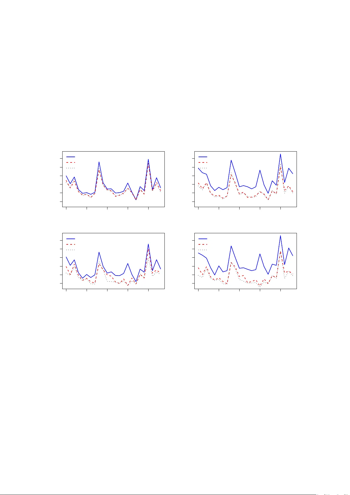
Zero V ariance P ortfolio Jin yuan Chang ∗ Yi Ding † Zhen tao Shi ‡ Bo Zhang § Abstract When the n umber of assets is larger than the sample size, the minimum v ari- ance p ortfolio in terp olates the training data, delivering pathological zero in-sample v ariance. W e show that if the weigh ts of the zero v ariance portfolio are learned b y a nov el “Ridgelet” estimator, in a new test data this portfolio enjo ys out-of-sample generalizabilit y . It exhibits the double descent phenomenon and can ac hieve optimal risk in the o verparametrized regime when the num b er of assets dominates the sam- ple size. In con trast, a “Ridgeless” estimator whic h in vok es the pseudoinv erse fails in-sample interpolation and div erges aw ay from out-of-sample optimalit y . Extensiv e sim ulations and empirical studies demonstrate that the Ridgelet metho d p erforms comp etitiv ely in high-dimensional p ortfolio optimization. Keyw ords: F actor Mo del, Mac hine Learning, Minim um V ariance Portfolio, Risk Managemen t, Random Matrix Theory ∗ South western Univ ersity of Finance and Economics and Chinese Academ y of Sciences, E-mail: c hang jinyuan@swufe.edu.cn . † Univ ersity of Macau, E-mail: yiding@um.edu.mo . ‡ Corresp onding Author. The Chinese Universit y of Hong Kong, E-mail: zhen tao.shi@cuhk.edu.hk . § Univ ersity of Science and T echnology of China, E-mail: wb chpmp@ustc.edu.cn . 1 1 In tro duction Artiﬁcial intelligence (AI) and mo dern mac hine learning are increasingly used as deci- sion engines in ﬁnance, from automated in vestmen t management to institution-scale risk con trol. A deﬁning feature of these systems is that they are often trained in a data regime that is sim ultaneously information-rich and sample-p o or: decision mak ers can ac- cess thousands of correlated signals or assets, yet only a limited time series is a v ailable to learn stable actions. This raises a central issue in AI for ﬁnance and business decisions— ho w to design optimization and estimation pro cedures that can exploit high-dimensional information while deliv ering reliable out-of-sample (OOS) p erformance. Recen t adv ancemen ts in AI and machine learning in ﬁnance ha ve reshap ed ho w re- searc hers approach return prediction and asset pricing. Emerging ﬁnancial applications highligh t the beneﬁts of complex mo dels and o v erparameterization in capturing sophisti- cated mark et dynamics (e.g., Gu et al. 2020 , F an et al. 2022 , A vramo v et al. 2023 , Chen et al. 2024 ). Empirical evidence sho ws that highly parameterized mo dels can outp erform traditional dimension-reduction techniques, ev en when they in terp olate in-sample data. Kelly et al. ( 2024 ) sho w that mo del complexit y b eneﬁts the market return prediction, and Kelly et al. ( 2022 ) demonstrate that the “virtue of complexity” exists for a v ariet y of asset classes. Didisheim et al. ( 2023 ) pro vide theoretical analysis of this phenomenon in o verly parameterized asset pricing mo dels. F urthermore, in economic predictions, Liao et al. ( 2023 ) ﬁnd that Ridgeless regression that in terp olates in-sample data surpasses man y commonly used mo dels based on dimension reduction. This coun terintuitiv e success is closely tied to implicit regularization, where ov erpa- rameterized mo dels generalize well despite p erfect in-sample ﬁt. Machine learning theory oﬀers insights into this b ehavior: Hastie et al. ( 2022 ) sho w the double descen t b ehav- ior for Ridgeless regressions under a non-asymptotic setting. Bartlett et al. ( 2020 ) and T sigler and Bartlett ( 2023 ) establish the b enign of ov erﬁtting under the high-dimensional regime where the sample size is of the same order as the num b er of parameters. Cheng and Mon tanari ( 2024 ) further pro vide sharp guarantees for b enign o verﬁtting under high dimensional settings where the parameter space far exceeds the sample size. In this pap er, w e explore how mo dern insights from AI and machine learning can b eneﬁt complex p ortfolio optimization. Since Mark owitz ( 1952 ) introduced the mean- v ariance framework, this classic problem has faced persistent c hallenges that mirror those in mo dern machine learning. Practitioners op erate in a regime that they hav e limited time-series data to construct p ortfolios that span thousands of assets. W e fo cus on the 2 minim um v ariance portfolio (MVP) problem, whic h sits at the foundation of mo dern p ortfolio theory . It serv es as b oth a theoretical cornerstone and a practical default when return estimates are noisy . MVP is a simple constrained quadratic optimization. It provides the cleanest en viron- men t for in-depth analysis. Denote N as the num b er of assets o ver the cross section, and T as the sample size o ver the time dimension. Let r t = ( r 1 t , . . . r N t ) ⊤ b e an N -dimensional v ector of observ ed returns (with zero mean) at time t = 1 , . . . , T . W e assume that r t is stationary ov er time, and the p opulation cov ariance matrix Σ = E ( r t r ⊤ t ) is strictly p ositiv e deﬁnite. The w eigh t ω = ( ω 1 , . . . , ω N ) ⊤ assigned to the N assets m ust b e in the aﬃne h yp erplane ∆ N = { ω ∈ R N : 1 ⊤ ω = 1 } , where 1 is a column of N ones. W e allo w for short sells with ω i < 0 . W ere there an “oracle” that rev eals Σ , we would solv e the p opulation v ersion of MVP min ω ∈ ∆ N ω ⊤ Σ ω . The oracle weigh t admits a closed-form solution ω ∗ = ( 1 ⊤ Σ − 1 1 ) − 1 Σ − 1 1 , which leads to the oracle minim um v ariance ( 1 ⊤ Σ − 1 1 ) − 1 > 0 . In reality Σ is unobserv able. What the research has is an N × T data matrix R = ( r 1 , . . . , r T ) . A natural and common practice is to replace the p opulation Σ with the plain sample co v ariance matrix S 0 = T − 1 RR ⊤ to solv e min ω ∈ ∆ N ω ⊤ S 0 ω . (1.1) When S 0 is in vertible, which holds in general when N < T , the solution is b ω = 1 1 ⊤ S − 1 0 1 S − 1 0 1 . (1.2) In the classical asymptotic framework where N is ﬁxed and T → ∞ , under standard assumptions, the law of large num b ers ensures that S 0 con verges in probabilit y to Σ . When this happens, b ω con verges to the oracle weigh t ω ∗ asymptotically . Ho wev er, the ab o ve classical asymptotic framework do es not ﬁt the realit y of the ﬁnancial market w ell. As emphasized ab ov e, in vestors t ypically need to learn a high- dimensional p ortfolio based on training data with a relativ ely small sample size. F or instance, if we construct a p ortfolio that includes ab out 500 sto cks, say the S&P 500, and use the widely accessible daily data, then each month has only ab out 22 trading da ys—a short estimating window mak es trading strategies adaptiv e to the ev er-evolving mark et en vironment. In this case, w e are faced with the n umber of assets N at least t wen ty 3 times greater than the sample size T . This estimation problem should b e studied under a high-dimensional setting where the cross section can be m uch larger than the sample size. In the ﬁnancial w orld, “ N > T ” or more precisely “ N ≫ T ”, is the norm, rather than the exception. The MVP literature has long recognized the c hallenges posed b y high dimensionalit y . It is well-kno wn that the plug-in estimator using sample cov ariance matrix do es not work satisfactorily when the dimension N is high; see, e.g., Mic haud ( 1989 ), Kan and Smith ( 2008 ) and Ao et al. ( 2019 ). T o address this, v arious studies hav e prop osed alternative co v ariance matrix estimators. F or example, Caner et al. ( 2025 ) prop ose the no dewise regressions for the precision matrix, Caner et al. ( 2024 ) carry constraints in to p ortfolio analysis, and Ding et al. ( 2021 ) adopt a threshold-t yp e estimator under factor mo dels. Shrink age estimators are widely used in practice ( Ledoit and W olf 2003 , 2004 , 2017 ), and their theoretical properties are justiﬁed when N and T are of the same order. The prev ailing wisdom in the MVP literature is clear: a void the naive sample co- v ariance matrix S 0 in high dimensions; instead, use sophisticated estimators suc h as shrink age, factor-based metho ds, or regularization tec hniques. Decades of research ha ve reinforced this principle. Y et, in this pap er, w e challenge this ortho do xy . Inspired by recen t adv ances in AI and mac hine learning, w e ask: In the N ≫ T r e gime, c ould a simple appr o ach b ase d on the sample c ovarianc e matrix lever age the rich cr oss-se ctional information, despite the sc ar city of temp or al observations, to c onstruct a p ortfolio that gener alizes wel l to out-of- sample data? Our answer is a surprisingly simple yet no vel idea for estimating the weigh ts. Pic k a small p ositiv e real num b er, for example 10 − 8 , and call it τ . Our prop osed weigh t estimator is b ω τ = 1 1 ⊤ S − 1 τ 1 S − 1 τ 1 with S τ = S 0 + τ I N , (1.3) where I N is the iden tity matrix. The solution in ( 1.3 ) diﬀers from ( 1.2 ) only in that w e add a tin y “ridge” to the sample cov ariance matrix S 0 . W e name this estimator R idgelet . There is gro wing in terest in p ortfolio optimization with ridge-t yp e penalties (e.g., Bo dnar et al. ( 2018 , 2022 , 2024 ) and Meng et al. ( 2025 )), but Ridgelet should not b e tak en as ridge-t yp e regularization. The standard ridge uses τ > 0 as a tuning parameter to balance the bias and v ariance. In practice, the tuning parameter is chosen either b y cross v alidation from a grid of user-sp eciﬁed v alues, or by Ledoit and W olf ( 2004 )’s b ona 4 ﬁde linear shrink age. In con trast, our τ is a tiny pre-sp eciﬁed constan t that remains in v arian t with N and T . Throughout this pap er’s Monte Carlo sim ulations and empirical applications, we ﬁx it at 10 − 8 , and the results are robust if w e change it to other small v alues, say 10 − 10 . W e view the Ridgelet estimation as a tuning-free device to guide the w eights ω , which will b e made clear in Prop osition 1 ; it is not a tuning parameter to impro ve the estimation quality of S 0 . Ridgelet is motiv ated by in-sample in terp olation. When N > T , in general there exists some ω ∈ ∆ N that pro duces an in-sample zer o varianc e p ortfolio (ZVP) ω ⊤ S 0 ω = 0 . It transpires that Ridgelet constructs a particular case of ZVP b y minimizing the Euclidean norm of ω . Con ven tionally , ZVP is viewed as a pathological case b ecause the in-sample v ariance drops b elow the oracle p opulation v ariance ( 1 ⊤ Σ − 1 1 ) − 1 . In other w ords, ZVP m ust hav e overﬁtte d the training data. In the standard framew ork of the bias-v ariance tradeoﬀ, ov erﬁtting fails to generalize to a test dataset, leading to p o or OOS p erformance. In recen t years, how ev er, this pi ece of con ven tional wisdom has b een challenged when AI researchers witnessed that deep neural net works with h undreds or thousands of times more parameters than training examples w ere achieving state-of-the-art generalization, and larger models contin ued to deliv er b etter test p erformance. T o describ e the interactions b et ween generalizability and mo del complexit y , Belkin et al. ( 2020 ) use double desc ent to refer to the phenomenon where the test error of a mo del displays tw o distinct regimes of descent as mo del complexit y increases. Our Ridgelet p ortfolio features the double descent in its risks. W e illustrate such a pattern in the left panel of Figure 1 . W e draw the p ortfolio risk (black solid curve) against the num b er of assets N while keeping the sample size ﬁxed at T = 22 . The p ortfolio OOS risk ﬁrst decays as N gro ws from a small v alue 2 to 10, that is, the ﬁrst descen t. Then it rapidly gro ws as N approaches T . As N go es beyond T , the risk dips again in a second descen t. On the other hand, when N > T the in-sample risk (red dotted curve) lies ﬂat at essen tially zero. 5 0 5 10 15 20 25 30 Number of Assets N (log scale) P or tfolio Risk 2 5 10 20 50 100 500 Ridgelet in−sample risk oracle MVP sample size T 0 5 10 15 20 25 30 Number of Assets N (log scale) P or tfolio Risk 2 5 10 20 50 100 500 Ridgeless in−sample risk oracle MVP sample size T Figure 1: Risk curv e of the MVP estimated with Ridgelet (left) and Ridgeless (righ t). The oracle minim um risk is a b enc hmark. The returns are generated from a factor mo del describ ed in Section 3.1 . In linear regressions, Hastie et al. ( 2022 ) pro vide a comprehensive analysis of double descen t for the Ridgeless estimator, whic h replaces the inv erse ( · ) − 1 of the Gram matrix in the usual OLS estimator with the Mo ore-Penrose pseudoin verse ( · ) + . In p ortfolio analysis, the sample cov ariance S 0 m ust be rank-deﬁcien t when N > T , and S 0 = lim τ → 0 S τ . In mean-v ariance p ortfolios, Lu et al. ( 2024 ) use this pseudoin verse to demonstrate double descen t in the Sharpe ratio. In our con text of MVP , one ma y b e tempted to mimic the Ridgeless regression estimator b y w orking with b ω + = 1 1 ⊤ S + 0 1 S + 0 1 , (1.4) whic h we call the Ridgeless weigh t in this pap er. Unlik e the regression problem, the Ridgelet b ω τ in ( 1.3 ) and the Ridgeless b ω + in ( 1.4 ) are fundamen tally diﬀerent estimators in MVP , and w e are against the use of Ridgeless in the regime N > T (see Proposition 1 and Remark 2 in Section 2.2 ), for S − 1 τ suﬀers discon tinuit y at the τ = 0 . T o intuitiv ely witness that Ridgeless is an undesirable estimator, in the right panel of Figure 1 we draw its risk with the same data as in the left panel. The OOS risk proﬁle of Ridgeless (blac k solid curv e) is the same as Ridgelet when N < T . How ev er, after a quick second descen t when N exceeds T , the risk of Ridgeless div erges from the oracle coun terpart when N b ecomes larger than 50. Moreo ver, when N > T the in-sample risk (red dotted curv e) rises again—it does not interpolate the training data, thereb y not a ZVP . In real-world ﬁnancial mark ets, sto ck returns are driven b y common factors at the o verall mark et level, as well as correlations at a lo calized level from industries and supply 6 c hains. A lo w-rank factor structure with a sparse idiosyncratic co v ariance matrix is commonly used to charac terize the comov ements (e.g., Ding et al. 2021 , Du et al. 2023 ). T o b etter absorb information from the lo cal lev el, we prop ose a reﬁned version of the Ridgelet estimator. The reﬁned Ridgelet estimator replaces the identit y matrix moun ted to the tiny ridge with a consisten t estimator of the idiosyncratic cov ariance matrix. T o b e sp eciﬁc, w e will attac h the tin y ridge to the threshold idiosyncratic cov ariance estimator b y F an et al. ( 2013 ). T o diﬀeren tiate the t w o versions of Ridgelet estimators, we refer to the v anilla Ridgelet in ( 1.3 ) as R idgelet1 , and the reﬁn ed copy as R idgelet2 (see ( 2.9 ) in Section 2.5 ). 1 W e sho w that when N ≫ T , Ridgelet2 improv es Ridgelet1 by securing optimality if the sto ck returns follo w an approximate factor mo del ( Cham b erlain and Rothschild 1983 ). Here “optimalit y” is deﬁned in the sense that the OOS risk of the p ortfolio constructed b y the w eights from Ridgelet2 asymptotically approaches the risk of the p opulation oracle (see Theorem 2 in Section 2.5 ). It b eneﬁts from the blessing of dimensionality ( Li et al. 2018 ). T o summarize, our theoretical con tributions are tw ofold. First, w e show that the ZVP estimated b y Ridgelet1 enjoys generalizability in new test data after passing the p eak of the complexit y regime, whereas the w ell-known Ridgeless estimator fails in-sample in terp olation and OOS extrap olation. Second, in the approximate factor mo del, we make it clear that optimalit y hinges on kno wledge of the idiosyncratic co v ariance matrix, and b y lev eraging a consistent estimator of it, Ridgelet2 can deliv er optimalit y in the high- dimensional case when N ≫ T . It is this pap er’s recommended estimator. Our asymptotic analysis relies on Random Matrix Theory (RMT). RMT is a principled to olkit for studying eigenv alue b eha vior and other high-dimensional phenomena in AI and mac hine learning, and has seen increasing adoption in econometrics; see, e.g., Onatski and W ang ( 2018 ), Kelly et al. ( 2022 ), Bykho vsk a ya and Gorin ( 2023 ) and He ( 2024 ). W e p erform extensive numerical studies to ev aluate the p erformance of the prop osed Ridgelet approac h. W e compare it with several b enchmark metho ds, including the linear shrink age (LS) estimator ( Ledoit and W olf 2004 ) and the factor-based nonlinear shrink age (FNLS) estimator ( Ledoit and W olf 2017 ). Using the S&P 500 Index constituents and Nikk ei 225 sto c ks, the Ridgelet metho d p erforms comp etitively . Ridgelet allows us to assign w eights to more than 700 sto cks with merely one mon th’s daily returns. 1 These names are inspired by “System 1” and “System 2” in the p opular science b o ok Thinking, F ast and Slow by Daniel Kahneman, a psychologist and Nob el laureate in economics. 7 Outline The rest of the pap er is organized as follows. Section 2 constructs the Ridgelet estimators and presents the main theoretical results. Sections 3 and 4 provide simulation studies and empirical applications, resp ectively . Concluding remarks are giv en in Section 5 . App endix A includes the pro ofs of Lemma 1 , and Prop ositions 1 and 2 . Pro ofs of the remaining theoretical statemen ts are collected in the online supplemen tary materials. Notations W e use the following notations throughout the pap er. A vector is a column b y default. F or a generic vector x = ( x i ) , we deﬁne its transp ose as x ⊤ , and its ℓ 2 norm as ∥ x ∥ = p P i x 2 i . F or a generic matrix A = ( A ij ) , we denote its sp ectral norm as ∥ A ∥ = max ∥ x ∥≤ 1 ∥ Ax ∥ , its minim um singular v alue as ∥ A ∥ min , and its trace as tr( A ) when A is a square matrix. The indicator function is denoted as I ( · ) . W e use “ p → ” to represen t conv ergence in probability . F or tw o sequences of p ositive real num b ers a n and b n , we write a n ≍ b n if b n /c ≤ a n ≤ cb n for some constan t c ≥ 1 , and write a n = o ( b n ) or a n ≪ b n if a n /b n → 0 . 2 Theory 2.1 Exact Solution to ZVP Zero V ariance Portfolio (ZVP) refers to the existence of a p ortfolio weigh t v ector ω ∈ ∆ N suc h that the in-sample v ariance ω ⊤ S 0 ω = 0 . Since S 0 is p ositiv e semi-deﬁnite b y construction, ZVP is equiv alent to existence of a solution to the linear ( T + 1) -equation system R ⊤ 1 ⊤ ! ω = 0 1 ! , (2.1) whic h is obviously an in-sample interpolation. Throughout the pap er, we assume 1 / ∈ span( R ) , that is, 1 is not a linear combination of the columns in R . It holds in general with probabilit y one when the entries in R are random. W e ﬁrst state a simple fact from linear algebra. Lemma 1 Supp ose 1 / ∈ span( R ) . If N = T + 1 , then a solution to ZVP ( 2.1 ) exists. If N ≥ T + 2 , ther e ar e inﬁnitely many solutions to ( 2.1 ) . 8 When ( 2.1 ) has multiple solutions, one may consider using a criterion to select one of them. Shi et al. ( 2025 ) prop ose minimizing the ℓ 2 -norm of the weigh t v ector. Indeed, if we set the tuning parameter in Shi et al. ( 2025 )’s ℓ 2 -r elaxation as zero, w e obtain the minim um ℓ 2 -norm ZVP problem min ω ∈ R N ∥ ω ∥ 2 sub ject to ( 2.1 ) . (2.2) Since all constrain ts are linear and the ob jective function is strictly conv ex, this program- ming problem has a unique solution. T o ﬁnd it, w e orthogonalize S 0 = U T Λ T U ⊤ T , (2.3) where Λ T is a diagonal matrix that stores the T eigen v alues of S 0 , and U T is an N × T matrix whose columns are the corresponding eigen vectors. Denote the pro jector to the n ull space of S 0 as P ⊥ S = I N − U T U ⊤ T . Then the exact solution to ( 2.2 ) is b ω exa = P ⊥ S 1 1 ⊤ P ⊥ S 1 . (2.4) Remark 1 The minimum ℓ 2 -norm ZVP estimator b ω exa in ( 2.4 ) and the Ridgeless esti- mator b ω + in ( 1.4 ) ar e fundamental ly diﬀer ent estimators. Using the notations in ( 2.3 ) , we c an r ewrite b ω + as b ω + = U T Λ − 1 T U ⊤ T 1 1 ⊤ U T Λ − 1 T U ⊤ T 1 . It is cle ar that the R idgeless estimator is determine d by the c olumn sp ac e of R , yet b ω exa is determine d by the nul l sp ac e of R , as shown in ( 2.4 ) . Inde e d, these two ve ctors ar e ortho gonal in the sense that their inner pr o duct b ω ⊤ exa b ω + = 0 b e c ause P ⊥ S U T = 0 . 2.2 The Ridgelet Estimator The minim um ℓ 2 -norm ZVP estimator b ω exa is diﬃcult to analyze b ecause the orthogo- nalization of S 0 cannot b e expressed as a simple closed-form function of the data. T o facilitate n umerical and asymptotic analysis, w e instead use Ridgelet1 in ( 1.3 ). The next prop osition sho ws that Ridgelet1 is an appro ximate solution to b ω exa . 9 Prop osition 1 F or a given data matrix R , assume that 1 / ∈ span( R ) . Then the Ridgelet1 estimator b ω τ in ( 1.3 ) solves the minimum ℓ 2 -norm ZVP ( 2.2 ) up to numeric al err ors. The Ridgeless estimator b ω + in ( 1.4 ) is not the solution to ( 2.2 ) . Prop osition 1 connects ZVP with Ridgelet1. The pro of sho ws that the Ridgelet esti- mator is the limiting solution to the Lagrangian dual of the primal problem ( 2.2 ). F or an y arbitrarily small ϵ > 0 , given the data matrix R , there exists a τ = τ ( ϵ ) = O ( √ ϵ ) suc h that b ω ⊤ τ S 0 b ω τ ≤ ϵ . The relationship b etw een τ and ϵ can b e strengthened to τ ≍ √ ϵ . A tin y τ in Ridgelet1 corresp onds to a tin y ϵ that mimics the limit ϵ → 0 . In tuitively , to elicit a unique solution from the inﬁnitely many solutions to ( 1.1 ), we use a strictly con v ex programming problem with a tiny ridge-t yp e p enalty: min ω ∈ ∆ N { ω ⊤ S 0 ω + τ ∥ ω ∥ 2 } . (2.5) The Ridgelet estimator ( 1.3 ) solves ( 2.5 ). Since the numerical computation of ω ⊤ S 0 ω con tains n umerical errors due to the ﬁnite precision in digital computers, in practice w e use τ = 10 − 8 , corresp onding to ϵ ≍ 10 − 16 . Remark 2 In a line ar r e gr ession, denote X as the T × N matrix of the r e gr essors and y as the T × 1 ve ctor of the dep endent variable. Hastie et al. ( 2022 ) study the interp olation pr oblem of a non-homo gene ous system of line ar e quations X β = y when N > T , whose minimum ℓ 2 -norm solution is the Ridgeless estimator b β = ( X ⊤ X ) + X ⊤ y = X ⊤ ( XX ⊤ ) − 1 y = lim τ → 0 X ⊤ ( XX ⊤ + τ I T ) − 1 y . Ther efor e, in line ar r e gr essions the Ridgelet would b e e quivalent to Ridgeless up to numer- ic al err ors, sinc e X ⊤ ( XX ⊤ + τ I T ) − 1 is c ontinuous at τ = 0 . The key diﬀer enc e of ZVP fr om the line ar Ridgeless r e gr ession is that, in our c ontext S + 0 1  = lim τ → 0 + ( S 0 + τ I N ) − 1 1 . Henc e b ω τ is disc ontinuous at τ = 0 . 2.3 Out-of-Sample V ariance No w that w e ha ve explored the in-sample prop erties of Ridgelet, what are its behaviors in a test dataset? W e will in vestigate this question in an asymptotic framework where 10 b oth N and T grow to inﬁnit y . Deﬁne V : ∆ N 7→ R + as the OOS varianc e of a generic w eight ω , giv en by V ( ω ) = ω ⊤ Σ ω . The oracle OOS v ariance is V ( ω ∗ ) = ( 1 ⊤ Σ − 1 1 ) − 1 . Since V ( ω ∗ ) ∈  ( N ∥ Σ ∥ ) − 1 , ( N ∥ Σ ∥ min ) − 1  , if all eigenv alues of Σ are b ounded a wa y from 0 and inﬁnit y , then V ( ω ∗ ) ≍ 1 / N . T o mea- sure ho w far V ( ω ) deviates from its oracle coun terpart, w e deﬁne the r elative (OOS) varianc e RV ( ω ) = V ( ω ) V ( ω ∗ ) = ω ⊤ Σ ω · 1 ⊤ Σ − 1 1 . Since no estimated metho d can ha v e lo wer OOS v ariance than the oracle, RV ( ω ) ≥ 1 in probabilit y . F rom Figure 1 w e ha v e observ ed that the OOS risk , formally deﬁned as p V ( ω ) , sho ws double descen t in Ridgelet as w ell as Ridgeless. How ev er, their risks b ehav e v ery diﬀeren tly when N ≫ T . The following prop osition pro vides a theoretical justiﬁcation for this phenomenon. Prop osition 2 Supp ose the data matrix is gener ate d by R = Σ 1 / 2 W , wher e ∥ Σ ∥ ≍ ∥ Σ ∥ min ≍ 1 , and W ( N × T matrix) c onsists of indep endently and identic al ly distribute d (i.i.d.) r andom variables with zer o me an, unit varianc e, and ﬁnite 4th moment. As N , T → ∞ and N /T → ∞ , ther e exists a ﬁnite c onstant C ≥ 1 such that Pr { RV ( b ω τ ) < C } → 1 for the Ridgelet estimator, wher e as RV ( b ω + ) p → ∞ for the Ridgeless estimator. Prop osition 2 ’s assumptions on R are the same as those in Hastie et al. ( 2022 , p.959). They allow us to in vok e RMT to obtain the sto chastic orders of the minim um and the maxim um eigen v alues of S 0 . This prop osition shows that V ( b ω τ ) is comparable to that of the oracle in its order, but Ridgeless’s relative v ariance div erges to inﬁnity , whic h is un- fa vorable. In comparison, notice that the equal-w eight (EW) p ortfolio with ω EW = 1 / N is alw ays av ailable without referring to an y data, and its OOS v ariance is V ( ω EW ) = 1 ⊤ Σ1 N 2 ≤ ∥ Σ ∥ N ≍ 1 N , so RV ( ω EW ) ≍ 1 . Hence, Ridgeless p erforms ev en worse than the EW p ortfolio. This negativ e result ab out Ridgeless formalizes the ca veat from Bo dnar et al. ( 2018 , 2022 ), whic h advises not using the pseudoin verse solution when N /T > 2 . 11 Remark 3 The MVP with ridge p enalty has b e en extensively studie d by Bo dnar et al. ( 2018 , 2022 , 2024 ). Inde e d, when N > T , Bo dnar et al. ( 2022 ) discuss the smal l ridge tuning p ar ameter τ → 0 ar ound the p e ak when N /T → 1 as a devic e to smo oth out the disc ontinuity b etwe en S − 1 0 and S + 0 . Bo dnar et al. ( 2024 ) pr op ose the double shrinkage appr o ach. Our p ap er distinguishes itself fr om them in the fol lowing asp e cts. First, these p ap ers take the ridge’s p enalty level τ as a tuning p ar ameter to b e optimize d; we inste ad stick to a ﬁxe d tiny τ , which is not a tuning p ar ameter. Se c ond, while these p ap ers c onsider N /T → (0 , ∞ ) , we enc our age a very lar ge N with N ≫ T to obtain the optimality of the Ridgelet appr o ach (se e Se ction 2.5 ). Both Prop ositions 1 and 2 are cautionary tales against the use of Ridgeless in p ortfolio optimization when N > T . The former sho ws that if w e are in terested in ZVP in the training data, it can b e appro ximated by Ridgelet1, but the Ridgeless is orthogonal to the exact solution. The latter sho ws that the relative v ariance of the Ridgeless is even w orse than EW. 2.4 F actor Structure in Co v ariance F actor mo dels are fundamentally imp ortant for ﬁnancial returns, as supp orted by nu- merous empirical studies. Figure 2 plots the top 10 eigenv alues of the sample co v ariance matrix of the S&P 500 constituent sto c ks. The ﬁrst sample eigen v alue clearly dominates all others in its magnitude. Supp ose that the sto ck return data matrix R follows a latent factor mo del of r factors R = BF + E , where an N × T matrix E represents the idiosyncratic returns, and it is indep endent of an r × T matrix of factors F = ( f 1 , . . . , f T ) . The factor f t is stationary o ver time, and as a normalization, E ( f t f ⊤ t ) = I r ; the associated factor loadings are enco ded in an N × r non-random matrix B . Decomp ose BB ⊤ = VΛ B V ⊤ = V diag ( λ B , 1 , . . . , λ B ,r ) V ⊤ , where λ B , 1 ≥ · · · ≥ λ B ,r are the r eigen v alues and the N × r matrix V consists of the corresp onding eigenv ectors. W e imp ose the following assumptions to facilitate asymptotic analysis. 12 2 4 6 8 10 0.0 0.1 0.2 0.3 0.4 0.5 0.6 Scree plot based on daily returns of S&P 500 Index stoc ks Component eigenv alue propor tion Figure 2: Scree plot of daily returns of S&P 500 Index Constituen t sto c ks. W e compute the sample co v ariance matrix of daily returns of S&P 500 Index sto c ks betw een 2020 and 2023. The Y-axis shows the ratios of its principal eigen v alues ov er the sum of all eigen v alues. Assumption 1 (i). L et Z b e an N × T matrix c onsisting of i.i.d. standar d Gaussian entries, and the idiosyncr atic r eturns E = Ω 1 / 2 Z , wher e ∥ Ω ∥ ≍ ∥ Ω ∥ min ≍ 1 . (ii). λ B , 1 ≍ λ B ,r ≍ N δ for some δ ∈ (0 , 1] and N δ ≫ 1 + N /T . Assumption 1 (i) requires that the idiosyncratic returns E is a linear transformation of i.i.d. en tries of Z . Admittedly , the Gaussianit y on Z is a strong assumption. It is a tec hnical condition to keep the theory simple when RMT is inv ok ed. It is p ossible to relax Gaussianit y b y imp osing some ﬁnite moment conditions instead, at the cost of subs tan tial complication of the notations and the proofs but adding little insigh t of the theoretical mec hanisms. There exist metho ds–—alb eit with cumbersome pro cedures—–in RMT to extend the normality assumption to general distributions. F or example, Knowles and Yin ( 2017 ) relax the conditions to any ﬁnite moment being b ounded. Ding and Y ang ( 2018 ) relax the conditions to the fourth momen t tail condition and d iagonal Ω , while Y ang ( 2019 ) remov es the diagonal restriction under the same tail condition. 2 Assumption 1 (ii) 2 In our Monte Carlo simulations, we c heck the p erformance of the portfolio risks under b oth the normal errors and hea vy-tailed errors, and the results are robust. 13 assumes that the r eigenv alues ha ve the same order of strength for simplicit y , and the div ergence of the factor strength separates the signal from the idiosyncratic returns in the approximate factor model. The divergence sp eed of the factor strength, which surely holds if N ≍ T , allo ws relatively weak factors. Under Assumption 1 , the population cov ariance matrix of r t is Σ = BB ⊤ + Ω , with r spiked eigen v alues of order N δ , and ( N − r ) non-spiked eigen v alues of order 1. By the S herman-Morrison-W oo dbury form ula ( Horn and Johnson 2012 , Eq.(0.7.4.1)), the oracle OOS v ariance is V ( ω ∗ ) = 1 1 ⊤ Ω − 1 / 2 [ I N − Ω − 1 / 2 VΛ 1 / 2 B ( I r + Λ 1 / 2 B V ⊤ ΩVΛ 1 / 2 B ) − 1 Λ 1 / 2 B V ⊤ Ω − 1 / 2 ] Ω − 1 / 2 1 . Clearly , it inv olv es V and Λ B from the factor comp onent and Ω from the idiosyncratic comp onen t. Deﬁne P ⊥ V = I N − VV ⊤ as the pro jector to the n ull space of B . The next assumption rules out the unlikely cases that the one-v ector 1 is in the r -dimensional linear space spanned b y V . Assumption 2 (i). ∥ P ⊥ V 1 ∥ / √ N ≫ p N (1 − δ ) /T . (ii). τ = o ( ∥ P ⊥ V 1 ∥ / √ N ) . Since √ N is the ℓ 2 norm of 1 , geometrically N − 1 / 2 ∥ P ⊥ V 1 ∥ is the sin( · ) of the an- gle b etw een the one-vector and the linear space spanned by the columns of V . Since Assumption 1 (ii) pushes N (1 − δ ) /T → 0 , Assumption 2 (i) trivially holds if the angle is non-degenerate, under whic h Assumption 2 (ii) also holds when we set τ as a tiny p ositive real n um b er. Assumption 2 (ii) is sp elled out for the completeness of the theory , while in practice w e do not tune τ . W e impose Assumption 2 not b ecause the estimator fails to w ork when it is violated. Instead, it makes the analysis interesting. If 1 ∈ span( V ) , then the systematic risk from the factors cannot b e diversiﬁed, and V ( ω ∗ ) is b ounded a wa y from 0. The eﬀect of Ω b ecomes negligible in the ﬁrst order asymptotics, and thus is an unin teresting case. Giv en the ab o ve assumptions, in the underparametrized regime, w e state the OOS v ariance V ( b ω ) (recall b ω is deﬁned in ( 1.2 )) and that of the Ridgelet. In the o verparame- 14 terized regime, b ω is not well-deﬁned and we present results of V ( b ω τ ) only . The expressions in Theorem 1 below in v olve the Stieltjes tr ansform , a fundamen tal ob ject in RMT. Let µ ( x ) b e the limiting spectral distribution of T − 1 Z ⊤ ΩZ . F or z ∈ C \ supp ( µ ) , the Stieltjes transform of µ ( x ) is deﬁned as m ( z ) = Z R 1 x − z d µ ( x ) . It is a smo oth enco ding of the eigen v alue distribution of the matrix, whic h conv erges to a deterministic limit and satisﬁes tractable equations. Notice that T − 1 Z ⊤ ΩZ is a p ositiv e semi-deﬁnite matrix. Th us, for an y z < 0 , w e ha ve z ∈ C \ supp ( µ ) . More- o ver, when N /T → γ ∈ (1 , ∞ ) , in probability T − 1 Z ⊤ ΩZ is of full rank, and supp ( µ ) is b ounded aw ay from zero and inﬁnity . Then m ( − τ ) is a p ositiv e b ounded num b er. When N /T → ∞ , b oth the upp er and low er b ounds of supp ( µ ) grow at rate N /T , whic h implies m ( − τ ) ≍ T / N . Theorem 1 Supp ose Assumptions 1 and 2 hold, and N , T → ∞ . (i). If N /T → γ ∈ (0 , 1) , then RV ( b ω ) p → 1 1 − γ and RV ( b ω τ ) p → 1 1 − γ . (ii). If N /T → γ ∈ (1 , ∞ ) , then V ( b ω τ ) = c ( τ ) · tr( Ω ) N · 1 + O p { d ( Ω ) } + o p (1) 1 ⊤ P ⊥ V 1 , (2.6) wher e d ( Ω ) = ∥ [ Ω − N − 1 tr( Ω ) I N ] P ⊥ V ∥ and c ( τ ) = 1 1 − T − 1 m 2 ( − τ )tr { [ I N + m ( − τ ) Ω ] − 2 Ω 2 } . Mor e over, if Ω = σ 2 I N with σ 2 ∈ (0 , ∞ ) , then RV ( b ω τ ) p → γ γ − 1 . (2.7) (iii). If N /T → ∞ , then V ( b ω τ ) V ( ω V ) p → 1 , (2.8) 15 wher e ω V = P ⊥ V 1 / ( 1 ⊤ P ⊥ V 1 ) . F urthermor e, if Ω = σ 2 I N , then RV ( b ω τ ) p → 1 . Theorem 1 (i) states the asymptotic prop erties of RV ( b ω ) and RV ( b ω τ ) in the regime N < T , where S 0 is of full rank. In this regime, the relative v ariance RV ( b ω ) monotonically in- creases in γ . In particular, when γ is close to 1, the relativ e v ariance explo des. The result also implies that V ( b ω ) tak es a familiar U-shap ed curve. Recall that V ( ω ∗ ) = ( 1 ⊤ Σ − 1 1 ) − 1 decreases in N . When N is muc h smaller than T , V ( b ω ) decreases as N increases; this is where the ﬁrst descen t app ears. In the regime N/T → γ ∈ (1 , ∞ ) , the expression ( 2.6 ) features multiple components, in particular the term c ( τ ) coming from limiting sp ectral analysis of RMT. The Stieltjes transform m ( z ) allows us to write the constants c ( τ ) in a closed, dimension-free form, turning random sp ectral ob jects in to deterministic limits. Here c ( τ ) ∈ [1 , ∞ ) . W e re- fer in terested readers to Theorem S.1 in the supplement, where a more accurate (and more complicated) asymptotic expression for V ( b ω τ ) is presented with additional nota- tion. Eq.( 2.6 ) implies that the diﬀerence b etw een Ω and I N pla ys an imp ortan t role. T o highligh t the rapid second descent after surpassing the interpolation threshold γ = 1 , w e presen t a simple expression ( 2.7 ) under the special case Ω = σ 2 I N . Theorem 1 (iii) is the limiting case when N ≫ T , under whic h the OOS v ariance V ( b ω τ ) con verges to V ( ω V ) . Here ω V can b e viewed as a factor-eliminating weigh t, b ecause V ⊤ ω V = 0 and thus V ( ω V ) = ω ⊤ V Σ ω V = ω ⊤ V Ω ω V . T o see the implications, consider the case ∥ P ⊥ V 1 ∥ / √ N ≥ c for some constant c ∈ (0 , ∞ ) , under whic h V ( ω V ) ≍ N − 1 . Given the asymptotic equiv alence, V ( b ω τ ) lev erages the ad- v antages brough t by high dimensionality when N is large. Since V ( ω ∗ ) ≥ ( 1 ⊤ Ω1 ) − 1 ≍ N − 1 , the optimal rate is ac hiev ed by V ( b ω τ ) . Under the factor mo del, this order of V ( b ω τ ) is in general m uch b etter than that of the EW p ortfolio. In fact, if ∥ V ⊤ 1 ∥ / √ N = cN − β for some β ∈ [0 , δ / 2) so that there is a non-trivial angle b etw een the one-vector and the column space of V , then the OOS v ariance under the EW sc heme is V ( ω EW ) = 1 ⊤ Σ1 N 2 ≥ c 2 N δ − 2 β − 1 ≫ 1 N ≍ V ( ω V ) . This inferior OOS v ariance from the EW sc heme is due to its complete disregard for the 16 presence of the factors. Ho wev er, when Ω  = σ 2 I N there is a gap b et ween V ( ω V ) and V ( ω ∗ ) , b ecause Ω shows up in ω ∗ but not in ω V , and ( 2.8 ) implies that the gap p ersists b etw een V ( b ω τ ) and V ( ω ∗ ) . In other w ords, V ( b ω τ ) is not optimal. This is understandable b ecause the tiny ridge p enalt y τ I N do es not align with a general Ω . Only in the sp ecial case Ω = σ 2 I N , the oracle p erformance can b e ac hiev ed b y V ( b ω τ ) , as stated in the second half of Theorem 1 (iii). This observ ation hints that, to ac hieve the oracle OOS v ariance in the general case, we m ust harness the information in Ω . This is what w e will do in the next section—upgrade Ridgelet1 to Ridgelet2. 2.5 Ridgelet2 T o ov ercome the drawbac k that Ridgelet1 ignores the cov ariance of the idiosyncratic returns, let us ﬁrst consider an infeasible scenario when Ω is known, so w e can work with a mo diﬁed v ersion of ( 2.2 ): min ω ∈ R N ∥ ω ∥ 2 sub ject to R ⊤ 1 ⊤ ! Ω − 1 / 2 ω = 0 1 ! . Again, this programming problem makes an in-sample ZVP , with the only diﬀerence b e- ing the presence of Ω − 1 / 2 in the constraints. It adjusts the add-to-one constrain t 1 ⊤ ω = 1 with equal w eight on eac h co ordinate into a w eighted version according to Ω − 1 / 2 1 . In the sp ecial case where Ω = diag( σ 2 1 , . . . , σ 2 N ) is diagonal and heterosk edastic, this trans- formation will put less w eigh t on a co ordinate with a larger σ 2 i . In the meantime, the original data v ector r t is transformed to Ω − 1 / 2 r t , which has a co v ariance matrix E ( Ω − 1 / 2 r t r ⊤ t Ω − 1 / 2 ) = Ω − 1 / 2 ΣΩ − 1 / 2 = Ω − 1 / 2 BB ⊤ Ω − 1 / 2 + I N . After the transformation, the co v ariance matrix of the idiosyncratic returns b ecomes an iden tity matrix I N . Applying the idea of Ridgelet to the transformed data would pro duce the oracle OOS v ariance, as hin ted by the second half of Theorem 1 (iii). If w e replace S τ = S 0 + τ I N with S τ , Ω = S 0 + τ Ω , w e pro duce e ω ifs τ = 1 1 ⊤ S − 1 τ , Ω 1 S − 1 τ , Ω 1 , 17 where the sup erscript “ifs” signiﬁes its infe asibility . T o make it useful in practice, w e m ust estimate the high-dimensional N × N matrix Ω . Given some sparse conditions, it is p ossible to obtain a consistent estimator b Ω for it. W e replace the infeasible S τ , Ω = S 0 + τ Ω with a feasible S τ , b Ω = S 0 + τ b Ω , and denote this feasible Ridgelet2 weigh t estimator as e ω τ = 1 1 ⊤ S − 1 τ , b Ω 1 S − 1 τ , b Ω 1 . (2.9) Theorem 2 Supp ose the assumptions in The or em 1 hold. As N , T → ∞ and N /T → ∞ : (i). The r elative varianc e of the infe asible estimator is RV ( e ω ifs τ ) p → 1 . (ii). The r elative varianc e of the fe asible estimator is RV ( e ω τ ) = 1 + O  ∥ Ω − b b Ω ∥  + o p (1) , wher e b = N − 1 tr( b Ω − 1 Ω ) . (iii). In addition, if ∥ b Ω − Ω ∥ = o p (1) , then RV ( e ω τ ) p → 1 . Theorem 2 (i) shows that V ( e ω ifs τ ) achiev es the oracle OOS v ariance, which is b etter than Ridgelet1. Result (ii) implies that whether the feasible e ω τ reac hes the oracle OOS v ariance hinges on the estimation quality of b Ω , measured by ∥ Ω − N − 1 tr( b Ω − 1 Ω ) b Ω ∥ . Since Ω is a high-dimensional cov ariance matrix, to consistently estimate it with limited sample size T , some structural conditions m ust b e imp osed for dimension reduction. A reasonable approach is to assume that, after removing the common factor comp onent, the dep endence among the remaining idiosyncratic comp onen ts are weak. Sparsity in the idiosyncratic co v ariance matrix is a widely adopted condition in practice (e.g., Ding et al. 2021 , Du et al. 2023 ). Theorem 2 (iii) provides a v eriﬁable condition ab out the estimation qualit y of b Ω for the optimalit y of the feasible estimator. Sp eciﬁcally , if b Ω is a consisten t estimator of Ω under the sp ectral norm, then e ω τ attains the oracle OOS v ariance. In the statistical literature, one widely used estimator that leverages idiosyncratic sparsit y in high-dimensional co v ariance matrices is F an et al. ( 2013 )’s principal orthog- 18 onal complemen t thresholding (POET). It applies adaptiv e thresholding on principal comp onen t analysis (PCA)-based residual cov ariance matrix estimator. T o mak e this pap er self-con tained, we brieﬂy describ e the POET pro cedure b elow. Algorithm: POET Input: Data matrix R . Output: b Ω Step 1. Compute S 0 = T − 1 RR ⊤ and p erform PCA on S 0 to decom- p ose it in to S 0 = P N i =1 λ i ξ i ξ ⊤ i , where λ 1 ≥ · · · ≥ λ N are the eigen v alues and { ξ i } N i =1 are the corresponding eigenv ectors. Step 2. Estimate r via the eigen v alue-ratio-based metho d ( Ahn and Horenstein 2013 ). Set b B = P r i =1 √ λ i ξ i and S u = ( ˆ σ ij ) = P N i = r +1 λ i ξ i ξ ⊤ i . Step 3. Threshold on S u to get b Ω = ( ˆ σ T ij ) with ˆ σ T ij = ˆ σ ij · I ( | ˆ σ ij | ≥ T ij ) . Here T ij = C 1 q ˆ θ ij η T with ˆ θ ij = T − 1 P T t =1 ( ˆ u it ˆ u j t − ˆ σ ij ) 2 , η T = ( r √ log N + r 2 ) / √ T + r 3 / √ N + p (log N ) /T , ˆ u it = (( I N − P r i =1 ξ i ξ ⊤ i ) R ) it , and C 1 > 0 a tuning parameter determined by 5-fold cross-v alidation to minimize the OOS v ariance for e ω τ . F or an idiosyncratic cov ariance matrix Ω = ( σ ij ) , deﬁne m N = max i ≤ N P N j =1 I ( σ ij  = 0) as the row-wise maxim um non-zero entries. F an et al. ( 2013 ) show that the ab ov e id- iosyncratic co v ariance matrix estimator satisﬁes ∥ b Ω − Ω ∥ = O p ( m N η T ) . (2.10) In our setting, η T = O ( p (log N ) /T ) . As long as the n umber of row-wise non-zero entries is not to o large in that m N = o ( p T / (log N )) , the POET estimator b Ω is consisten t under the sp ectral norm, and the optimalit y as stated in Theorem 2 (iii) is secured. W e will emplo y the POET estimator as describ ed ab o ve in the numerical w orks. 3 Sim ulation Studies In this section, we conduct n umerical sim ulations to c hec k the quality of asymptotic appro ximation. 3.1 Sim ulation Setting Our return data are generated from r t ∼ N (0 , Σ ) with t wo conﬁgurations of Σ : Setting 1: Σ = BB ⊤ + σ 2 I N (homosk edastic idiosyncratic returns). 19 Setting 2: Σ = BB ⊤ + Ω , where Ω is a sparse co v ariance matrix. The parameters are calibrated based on empirical data of the S&P 500 Index constituents— the last four y ears of test data in our empirical studies. Sp eciﬁcally , w e get the daily re- turns of the S&P 500 Index sto c ks b etw een 2020 and 2023, which include N 1 = 516 stocks in total, and compute its sample co v ariance matrix ˜ S = P N 1 i =1 λ i ξ i ξ ⊤ i , where λ 1 ≥ · · · ≥ λ N 1 and { ξ i } N 1 i =1 are the eigen v alues and the corresponding eigenv ectors of ˜ S . Based on Fig- ure 2 , we set the num b er of factors to r = 1 , and th us decomp ose ˜ S = λ 1 ξ 1 ξ ⊤ 1 + ˜ S u . W e then sp ecify B 1: N 1 = √ λ 1 ξ 1 for the ﬁrst N 1 assets. When N > N 1 , e.g., N = 1000 , we generate the loadings for the remaining assets B N 1 +1: N from Uniform [ b l , b h ] with b l and b h b eing the range of B 1: N 1 . T o construct the idiosyncratic cov ariance matrix, in Setting 1 w e make σ 2 = N − 1 1 P N 1 i =1 ( ˜ S u ) ii . F or Setting 2, we apply soft-thresholding to the oﬀ-diagonal elements of ˜ S u and get a sparse idiosyncratic cov ariance matrix block Ω 1: N 1 , 1: N 1 . If N > N 1 , new diagonal en tries diag( Ω N 1 +1: N ,N 1 +1: N ) are generated from Uniform [ σ l , σ h ] with σ l , and σ h b eing the range of the original N 1 assets. W e then select p ositions randomly from the remaining oﬀ-diagonal en tries of Ω based on the original sparsit y level in Ω 1: N 1 , 1: N 1 and ﬁll them with random co v ariance terms. The newly assigned non-zero idiosyncratic correlations are generated from a uniform distribution with ranges matched with that of the ﬁrst N 1 assets. Finally , w e apply soft-thresholding to the oﬀ-diagonal entries of Ω again to main tain the p ositiv e deﬁniteness of the full idiosyncratic cov ariance matrix Ω . W e simulate indep endent dra ws ov er t = 1 , . . . , T from the ab ov e mo dels and ev alu- ate ho w the p ortfolio p erforms when N increases. W e consider nested mo dels with an increasing cross-sectional dimension N = 400 , 600 , 800 , and 1000 . Regarding the time di- mension, we fo cus on the p erformance with a small T b ecause it represents a c hallenging, y et empirically relev ant scenario. Since the en vironment and sentimen t of the mark et ev olve ov er time, it is adv antageous to main tain a short inv estmen t horizon and learn in vestmen t strategies based on the most recent data, as highlighted in Didisheim et al. ( 2023 ). In b oth the sim ulation and the pro ceeding empirical applications, w e learn the p ortfolio w eights with T = 22 (44 , 63) , corresp onding to one mon th (tw o mon ths, three mon ths) of training data with daily returns. W e sim ulate the data for 1000 indep endent replications. In each replication, w e es- timate the weigh ts and ev aluate the p ortfolio p erformance in the relative (OOS) risk (RR): RR ( ω ) = p RV ( ω ) − 1 . 20 0 1 2 3 4 5 6 Number of Assets N (log scale) Relative Risk 5 10 20 50 200 500 Ridgelet sample size T 20 50 100 200 500 1000 0 1 2 3 4 5 6 Sample Size T (log scale) Relative Risk Ridgelet number of assets N Figure 3: Relative Risk curv es of Ridgelet. In the left panel, w e draw the mean relativ e risks for v arious N s and ﬁxed sample size T = 22 . In the righ t panel, we draw the mean relative risks for v arious T s and ﬁxed dimension N = 500 . The mean relative risk is computed as the a v erage from 10 replications. W e use Setting 2, where the idiosyncratic co v ariance matrix is a sparse matrix. The low er b ound of RR is 0. The closer to 0 is this num b er, the b etter is the p erformance. 3.2 Illustration of Double Descen t of Ridgelet In Section 1 , w e ha ve sho wcased in Figure 1 the in-sample and OOS risks of Ridgelet1 against the num b er of assets N while keeping the sample size T = 22 ﬁxed. W e used Setting 2, where the idiosyncratic co v ariance matrix is a sparse matrix. The double descen t patterns for diﬀerent settings are similar. In Figure 3 , we draw the RRs of Ridgelet1 against t wo dimensions, gro wing N while k eeping the sample size ﬁxed at T = 22 (left panel), and gro wing T while keeping the dimension ﬁxed at N = 500 (righ t panel). In the left panel, as the num b er of assets N increases, RR initially rises, p eaking at N = T , and then declines. T o wards the large cross section N = 1000 , RR go es up again. This do es not con tradict our theory which w orks under the asymptotics with N , T → ∞ , but in this ﬁgure, T is ﬁxed whereas N k eeps increasing. In the right panel, w e observ e the curve with respect to T . Holding N ﬁxed, RR p eaks at T = N , and clim bs down in either direction as T b ecomes smaller or greater than N . Based on the messages con v eyed in Figures 1 and 3 , the double descen t phenomenon can be explained in the following stages. First, in the regime N < T , as N gro ws from a small v alue, the oracle risk drops faster, dominating the growing RR of the estimator. This 21 leads to the ﬁrst descen t of the p ortfolio risk of Ridgelet. Second, when N approaches T , RR of the estimator increases drastically , dominating the eﬀect of the diminishing oracle risk. This results in a p eak at N = T . Finally , when N surpasses T , both RR and the oracle risk decline, leading to the second descent. 3.3 Ov erall P erformance W e ev aluate the p erformance of Ridgelet1 and Ridgelet2, in comparison with Ledoit and W olf ( 2004 )’s LS, Ledoit and W olf ( 2017 )’s FNLS, and the EW p ortfolio ( DeMiguel et al. 2009 ) as b enchmarks. T o b etter understand the n umerical prop erties of Ridgelet2, w e hold out a separate sample of size T 0 to estimate Ω . As expected, the larger is the held-out sample size, the b etter is the estimation quality of b Ω . In the tables b elow, w e will rep ort those under T 0 = 63 . W e do not resort to the held-out sample in empirical applications in Section 4 . W e display the RRs in T ables 1 and 2 . Given the presence of the factors, in all settings EW do es not w ork w ell, as it fails to div ersify the risk stemming from the factors. F or a ﬁxed training window T , e.g., T = 22 , as N increases from 400 to 1000 , because risks are b etter diversiﬁed with large N , all metho ds except EW enjo y lo wer RRs. As N increases, the RR of Ridgelet1 drops muc h faster and outp erforms LS for large N , e.g., N ≥ 400 . In Setting 1, the idiosyncratic cov ariance matrix is exactly a multiple of the iden- tit y matrix. The o verall b est p erformer is Ridgelet1. This is not surprising from our theoretical prediction of optimality . Indeed, in this setting Ω is indeed a multiple of the iden tit y matrix. With a data-driv en tuning parameter, LS is not as eﬀective as Ridgelet1. Similarly , although Ridgelet2 is asymptotically as eﬃcien t as Ridgelet1, the es- timated b Ω inﬂicts sampling errors, which slightly aﬀect its ﬁnite sample p erformance when T = 22 . Under T = 44 or 63 , its p erformance is impro ved substantially . When T = 63 and N ≤ 800 , FNLS is the winner. The relative p erformance of tuning-free Ridgelet1 declines when T gets closer to N . In T able 2 , Setting 2 has a nonzero sparse idiosyncratic co v ariance matrix. Here Ridgelet1 still outp erforms LS. The o verall b est p erformer is Ridgelet2, which tak es Ω in to consideration. Its adv antage is particularly salien t under a large N , e.g., N ≥ 800 , surpassing FNLS. These observ ations corrob orate our theoretical results of asymptotic optimalit y of the Ridgelet2 estimator. 22 T able 1: Risk p erformance under Setting 1. The mean and standard deviation (in the parenthesis) of RR of v arious portfolios from 1000 replications are reported. The smallest mean risk in eac h setting is sho wn in b old. Setting 1: Σ = BB ⊤ + σ 2 I N T N Ridgelet1 Ridgelet2 LS FNLS EW 22 400 0.945 (0.396) 0.973 (0.397) 1.068 (0.559) 1.002 (0.402) 7.548 600 1.051 (0.467) 1.072 (0.465) 1.120 (0.588) 1.103 (0.473) 11.382 800 1.041 (0.491) 1.111 (0.517) 1.084 (0.508) 1.086 (0.495) 15.899 1000 1.099 (0.524) 1.975 (0.955) 1.135 (0.538) 1.140 (0.527) 19.401 44 400 0.360 (0.131) 0.399 (0.140) 0.396 (0.145) 0.381 (0.144) 7.548 600 0.374 (0.147) 0.410 (0.154) 0.395 (0.154) 0.397 (0.154) 11.382 800 0.354 (0.147) 0.384 (0.153) 0.369 (0.152) 0.373 (0.155) 15.899 1000 0.366 (0.152) 0.397 (0.166) 0.378 (0.155) 0.385 (0.159) 19.401 63 400 0.237 (0.075) 0.267 (0.082) 0.248 (0.083) 0.215 (0.087) 7.547 600 0.225 (0.085) 0.245 (0.086) 0.234 (0.089) 0.217 (0.092) 11.382 800 0.204 (0.084) 0.230 (0.088) 0.210 (0.086) 0.201 (0.089) 15.899 1000 0.206 (0.088) 0.224 (0.088) 0.212 (0.090) 0.207 (0.091) 19.400 T able 2: Risk p erformance of MVPs under Setting 2. Setting 2: Σ = BB ⊤ + Ω T N Ridgelet1 Ridgelet2 LS FNLS EW 22 400 0.932 (0.315) 0.839 (0.318) 0.963 (0.319) 0.803 (0.283) 6.363 600 1.336 (0.456) 1.096 (0.413) 1.359 (0.459) 1.085 (0.386) 9.326 800 1.943 (0.637) 1.230 (0.480) 1.968 (0.640) 1.236 (0.459) 12.961 1000 2.439 (0.786) 1.305 (0.524) 2.465 (0.788) 1.327 (0.508) 16.026 44 400 0.514 (0.106) 0.414 (0.116) 0.522 (0.110) 0.415 (0.100) 6.363 600 0.684 (0.147) 0.511 (0.151) 0.693 (0.150) 0.536 (0.132) 9.326 800 0.951 (0.216) 0.540 (0.166) 0.962 (0.218) 0.582 (0.151) 12.961 1000 1.172 (0.266) 0.559 (0.180) 1.184 (0.268) 0.600 (0.161) 16.026 63 400 0.431 (0.069) 0.329 (0.068) 0.428 (0.071) 0.317 (0.065) 6.363 600 0.539 (0.091) 0.373 (0.085) 0.542 (0.093) 0.397 (0.084) 9.326 800 0.707 (0.128) 0.381 (0.098) 0.712 (0.129) 0.421 (0.095) 12.961 1000 0.847 (0.159) 0.386 (0.100) 0.854 (0.161) 0.428 (0.099) 16.026 23 3.4 Robustness to Hea vy-tailed Distribution The simulation results in T ables 1 and 2 are based on data that follo w the normal dis- tribution. Financial data, how ev er, often exhibits hea vy-tailedness. Though heavy-tailed distributions are not co vered by our Theorems 1 and 2 for the conv enience of the theo- retical dev elopment, w e use simulations here to chec k how the p erformance is aﬀected by hea vy-tailed distributions. T o in vestigate this, we generate R = Σ 1 / 2 W , where eac h en try of W is i.i.d. t - distributed with the degree-of-freedom b eing 5 , denoted b y t 5 . W e adopt the same co- v ariance matrix settings as b efore and rep ort the RRs in T ables 3 and 4 . Ridgelet1 and Ridgelet2 still p erform w ell and generate low er risks than the b enchmarks in v arious sce- narios. The results demonstrate robustness of our prop osal to heavy-tailed distributions. W e observe that when T = 63 (the maximum T in the simulations), Ridgelet2 exhibits an opp osite trend in Setting 1 (T ables 1 and 3) and Setting 2 (T ables 2 and 4). Sp eciﬁcally , its performance impro ves as N increases under Setting 1, while it deteriorates as N increases under Setting 2. A k ey reason stems from ( 2.10 ): under Setting 1, m N is alw a ys equal to 1, whereas under Setting 2, m N increases with N , thereb y leading to an inﬂated error. 4 Empirical Applications A ccording to p opulation form ulation, div ersiﬁcation is a “free lunch” that reduces the risk in the ﬁnancial market. Given a large num b er of inv estable assets, we m ust devise a sc heme to enjoy the free lunc h. In our real data applications, w e ﬁrst apply Ridgelet to the S&P 500 Index constituents. Next, w e extend the scop e to multinational inv estmen t opp ortunities b y incorp orating the Japanese Nikk ei 225 data. 4.1 S&P 500 Index Sto cks W e collect the daily returns of the S&P 500 sto c ks b et w een January 1999 and Decem- b er 2023. At the b eginning of each mon th, w e use the historical returns of the constituent sto c ks for the past T days to estimate the MVP weigh ts. W e use the sto c ks that p os- sess complete observ ations in the training windo w and construct p ortfolios with sample sizes T ∈ { 22 , 44 , 63 } days, as in the sim ulations. W e track the OOS daily returns of the p ortfolio for one mon th. W e re-estimate the weigh ts ev ery month. 24 T able 3: Risk p erformance of MVPs under Setting 1 and heavy-tailed distri- bution. Data are generated from t 5 . The mean and standard deviation (in paren theses) of RR of v arious portfolios from 1000 replications are rep orted. The smallest mean risk in eac h setting is sho wn in b old. Setting 1: Σ = BB ⊤ + σ 2 I N T N Ridgelet1 Ridgelet2 LS FNLS EW 22 400 0.965 (0.410) 0.962 (0.377) 1.117 (0.489) 0.932 (0.381) 7.548 600 1.072 (0.479) 1.057 (0.435) 1.151 (0.516) 1.016 (0.442) 11.382 800 1.069 (0.506) 1.046 (0.465) 1.121 (0.527) 1.002 (0.462) 15.899 1000 1.124 (0.535) 1.098 (0.492) 1.167 (0.551) 1.044 (0.485) 19.401 44 400 0.362 (0.137) 0.406 (0.137) 0.415 (0.163) 0.366 (0.138) 7.548 600 0.375 (0.155) 0.419 (0.151) 0.403 (0.166) 0.379 (0.149) 11.382 800 0.356 (0.159) 0.394 (0.151) 0.374 (0.165) 0.360 (0.148) 15.899 1000 0.368 (0.164) 0.403 (0.156) 0.383 (0.169) 0.371 (0.152) 19.401 63 400 0.240 (0.076) 0.287 (0.077) 0.257 (0.090) 0.219 (0.083) 7.548 600 0.226 (0.086) 0.273 (0.084) 0.238 (0.092) 0.221 (0.087) 11.382 800 0.206 (0.087) 0.252 (0.085) 0.214 (0.090) 0.207 (0.085) 15.899 1000 0.207 (0.090) 0.250 (0.088) 0.214 (0.093) 0.212 (0.087) 19.401 T able 4: Risk p erformance of MVPs under Setting 2 and heavy-tailed distri- bution. Setting 2: Σ = BB ⊤ + Ω T N Ridgelet1 Ridgelet2 LS FNLS EW 22 400 0.951 (0.324) 0.825 (0.301) 0.997 (0.333) 0.769 (0.272) 6.363 600 1.344 (0.463) 1.084 (0.386) 1.382 (0.472) 1.026 (0.370) 9.326 800 1.961 (0.652) 1.212 (0.455) 2.002 (0.659) 1.163 (0.440) 12.961 1000 2.462 (0.803) 1.289 (0.494) 2.507 (0.811) 1.241 (0.484) 16.026 44 400 0.516 (0.110) 0.414 (0.110) 0.529 (0.117) 0.405 (0.098) 6.363 600 0.682 (0.157) 0.511 (0.144) 0.697 (0.162) 0.518 (0.131) 9.326 800 0.952 (0.227) 0.541 (0.161) 0.971 (0.232) 0.560 (0.151) 12.961 1000 1.177 (0.284) 0.559 (0.169) 1.199 (0.289) 0.577 (0.161) 16.026 63 400 0.429 (0.066) 0.329 (0.065) 0.428 (0.079) 0.315 (0.058) 6.363 600 0.540 (0.090) 0.370 (0.083) 0.544 (0.095) 0.394 (0.078) 9.326 800 0.711 (0.130) 0.379 (0.093) 0.720 (0.134) 0.416 (0.089) 12.961 1000 0.850 (0.161) 0.382 (0.097) 0.863 (0.165) 0.423 (0.095) 16.026 25 2000 2005 2010 2015 2020 0.05 0.15 0.25 Ridgelet1: T=22 Y ear P or tfolio Risk N=100 N=300 N=500 2000 2005 2010 2015 2020 0.05 0.15 0.25 Ridgelet1: T=63 Y ear P or tfolio Risk N=100 N=300 N=500 2000 2005 2010 2015 2020 0.05 0.15 0.25 Ridgelet2: T=22 Y ear P or tfolio Risk N=100 N=300 N=500 2000 2005 2010 2015 2020 0.05 0.15 0.25 Ridgelet2: T=63 Y ear P or tfolio Risk N=100 N=300 N=500 Figure 4: Time-series of risks of MVPs b et ween 2000 and 2023, learned with diﬀeren t n umbers of sto cks. W e draw the ann ualized risks of MVP for N = 100 , 300 and 500 using the largest sto cks b y their capitalization. W e include the Ridgelet1 (top) and Ridgelet2 (bottom) p ortfolios for training window T = 22 and T = 63 . 26 W e ﬁrst ﬁx a training windo w T and examine how the risk b y Ridgelet1 or Ridgelet2 v aries with the n um b er of sto c ks N . T o do so, w e select the largest N = 100 , 300 , and 500 sto cks in the S&P 500 Index, sorted b y their capitalization, and construct MVP with these nested subsets of sto cks. Figure 4 presen ts the annualized risk proﬁles of the Ridgelet1 and Ridgelet2 p ortfolios. W e observ e a notable deduction in risks of b oth Ridgelet1 and Ridgelet2 when N gro ws from 100 to 300 . When N increases from 300 to 500 , the impro vemen t is small for Ridgelet1, while that for Ridgelet2 is still visible, in particular follo wing the tw o p eaks in the aftermath of 2008 ﬁnancial crisis and 2020 Co vid depression. The ov erall risk is rep orted in P anel A of T able 5 . Ridgeless do es not work w ell and even underp erforms EW with small T . All other data-driven metho ds—Ridgelet1, Ridgelet2, LS and FNLS—clearly b eat EW. It implies that when w e are able to track the constituent sto cks, EW is not a comp etitive alternative. While Ridgelet1 and LS explore the factor structure, Ridgelet2 and FNLS further utilize the information in the idiosyncratic comp onent to attain risk reduction. Ridgelet2 p erforms b etter than FNLS with a small margin. It app ears that Ridgelet1 aligns with LS. In the real data, the b one ﬁde estimator of LS pro duces a tuning parameter so small that it appro ximates our tuning-free Ridgelet1 estimator. On the other hand, Ridgelet2 p erforms closely to FNLS. Theoretically optimal among the r otation-e quivariant -t yp e estimators, FNLS is kno wn to b e one of the strongest estimators in S&P 500 ( Ledoit and W olf 2017 , Ding et al. 2021 , Jiang et al. 2024 ). The equally strong p erformance of Ridgelet2 reveals the gain of utilizing the sparsity of the co v ariance of the idiosyncratic comp onen t. When N > T , Ledoit and W olf ( 2017 , Eq.(15)) use a formula to pro vide a uniform adjustment for the zero sample eigenv alues. Ridgelet2 reveals that what is imp ortant is the presence of a small ridge that aligns with the true Ω , but optimal tuning is not necessary . Our Ridgelet2 is a ﬂexible framework that allows users to plug in their preferred consisten t estimator to explore the structure of the problems under in v estigation. 4.2 Multinational P ortfolio: S&P 500 plus Nikk ei 225 T o harvest the blessing of dimensionality , w e augment the U.S. data with Japanese data. Sp eciﬁcally , w e build m ultinational p ortfolios by enlarging the p o ol of the S&P 500 Index sto c ks with the Nikk ei 225 Index constituen t stocks. The num b er of sto cks is hence brough t up to ab out N = 725 . In this exercise, w e follow the same estimation time 27 T able 5: Risk p erformance of MVPs o ver Jan uary 2000 to Decem b er 2023. The rep orted quan tities are the ann ualized risk. In P anel A, we construct the MVP p ortfolio using daily returns of S&P 500 Index constituen t sto cks. In Panel B, w e construct m ultinational p ortfolios using b oth S&P 500 Index sto cks and Nikkei 225 Index sto cks. The lo west risk in each setting is highlighted in b old. T raining window Ridgelet1 Ridgelet2 LS FNLS EW Ridgeless P anel A: S&P 500 Sto c ks T = 22 0.122 0.097 0.135 0.099 0.213 0.226 T = 44 0.125 0.094 0.126 0.096 0.213 0.274 T = 63 0.122 0.098 0.122 0.099 0.213 0.155 P anel B: S&P 500 plus Nikk ei 225 Sto cks T = 22 0.115 0.086 0.114 0.087 0.176 0.318 T = 44 0.108 0.082 0.108 0.083 0.174 0.179 T = 63 0.103 0.082 0.104 0.083 0.175 0.251 framew ork as that in the S&P 500 data. A t eac h estimation p oin t, w e include the same S&P 500 sto c ks as in Panel A of T able 5 ; in addition, w e incorp orate the Nikkei 225 Index sto c ks that ha ve at least 75% complete observ ations within the training windo w. As a result, the total n umber of inv olv ed sto c ks v aries sligh tly o ver diﬀeren t sample sizes T , thereb y the small v ariation in EW. W e summarize the total risks of the m ultinational inv estmen t in P anel B of T able 5 . Except for Ridgeless, the most salient observ ation is that, in ev ery case with an enlarge p o ol of assets, the correspon ding risks of all p ortfolios are reduced. Compared with the case that in vesting solely in the S&P 500 sto c ks, the risk of Ridgelet2 for the m ultinational p o ol drops from 0.097 to 0.086 with a training windo w T = 22 . Moreov er, Ridgelet2 consisten tly outp erforms b oth Ridgelet1 and LS, and it maintains the small edge o ver FNLS. It exhibits robustness across v arying sample sizes and dimensionalities, making it a strong candidate for high-dimensional p ortfolio optimization with limited data. 28 5 Conclusion This pap er studies the generalizability of ZVP in test data. W e clarify when N > T the Ridgeless estimator inv olving the pseudoin verse S + 0 is not a prop er estimator for the MVP problem. W e deriv e the exact solution of the minim um ℓ 2 -norm ZVP and propose a nov el Ridgelet estimator as an easy-to-implemen t surrogate for it, where a tin y ridge a voids the discontin uit y of the pseudoin v erse corresp onding to Ridgeless with a zero ridge p enalt y . W e use RMT to analyze the limiting b ehavior of Ridgelet in a high-dimensional regime where the num b er of sto cks N can b e muc h larger than the size of the training sample T . W e obtain the limiting OOS v ariance of Ridgelet relativ e to the oracle OOS v ariance when the sto c k returns follow an approximate factor mo del. The theoretical analysis motiv ates a reﬁnemen t by incorp orating the idiosyncratic cov ariance matrix estimator Ω . W e show that when Ω can is estimated consistently , the reﬁned Ridgelet2 metho d attains the oracle OOS v ariance. Extensiv e sim ulations and empirical applications to S&P 500 Index constituen ts and Nikk ei 225 sto cks demonstrate the comp etitiv e p erformance of the Ridgelet idea. App endix A Pro ofs A.1 Pro of of Lemma 1 When N = T + 1 and rank( R ) = T , the N × N matrix  R 1  is inv ertible since 1 / ∈ span( R ) . The unique solution to ( 2.1 ) is ω = R ⊤ 1 ⊤ ! − 1 0 1 ! . If rank( R ) < T , then there are inﬁnitely man y solutions. When N ≥ T + 2 , we hav e rank( R ) ≤ T < N − 1 , and th us the ( T + 1) × N rectangular matrix  R 1  ⊤ implies inﬁnitely man y solutions to ( 2.1 ), as the num b er of free parameters is more than the num b er of linear restrictions. 29 A.2 Pro of of Prop osition 1 A natural relaxation to ( 2.2 ) is to replace the hard constrain t R ⊤ ω = 0 , whic h is equiv- alen t to ω ⊤ S 0 ω = 0 , b y a small upp er boun d on the v ariance: min ω ∈ ∆ N ∥ ω ∥ 2 sub ject to ω ⊤ S 0 ω ≤ ε, (A.1) for some prescrib ed ε > 0 . Eq.( 2.2 ) is the limit case of ( A.1 ) when ε → 0 + . This relaxation b y ε is to connect it with the familiar ridge-type metho d. W e in tro duce a Lagrange multiplier λ ≥ 0 for the inequalit y ω ⊤ S 0 ω ≤ ε and a m ultiplier µ ∈ R for the equalit y 1 ⊤ ω = 1 . The Lagrangian is L ( ω , λ, µ ) = ∥ ω ∥ 2 + λ  ω ⊤ S 0 ω − ε  + µ ( 1 ⊤ ω − 1) . F or ﬁxed ( λ, µ ) with λ ≥ 0 , the inﬁm um of L o ver ω i s g ( λ, µ ) = inf ω ∈ R N  ∥ ω ∥ 2 + λ ω ⊤ S 0 ω + µ 1 ⊤ ω  − λε − µ. The Lagrangian dual problem is max λ ≥ 0 , µ ∈ R g ( λ, µ ) . The inner inﬁm um o ver ω can b e equiv alently expressed by ﬁrst restricting to the aﬃne constrain t ∆ N : min ω ∈ ∆ N  ∥ ω ∥ 2 + λ ω ⊤ S 0 ω  . The dual problem is max λ ≥ 0  inf ω ∈ ∆ N  ∥ ω ∥ 2 + λ ω ⊤ S 0 ω  − λε  . Dropping the constan ts, the dual problem can b e equiv alently written as min ω ∈ ∆ N  ω ⊤ S 0 ω + 1 λ ∥ ω ∥ 2  , whic h is the Lagrangian dual of the constrained problem ( A.1 ). Solving the ab ov e ridge- t yp e problem yields the explicit solution b ω 1 /λ = S − 1 1 /λ 1 1 ⊤ S − 1 1 /λ 1 , where S 1 /λ = S 0 + λ − 1 I N . 30 Without loss of generality , let rank( S 0 ) = T , which admits a sp ectral decomp osition S 0 = U T Λ T U ⊤ T in ( 2.3 ). Let the N × ( N − T ) matrix U − T store the orthonormal columns spanning ker( S 0 ) . Let η T = U ⊤ T 1 b e the pro jection co eﬃcient of 1 onto the column space of S 0 , and η − T = U ⊤ − T 1 b e the pro jection co eﬃcient to the null space. Under the w eight ω 1 /λ , the in-sample v ariance is b ω ⊤ 1 /λ S 0 b ω 1 /λ = ∥ S 1 / 2 0 S − 1 1 /λ 1 ∥ 2 ( 1 ⊤ S − 1 1 /λ 1 ) 2 . When λ → ∞ , notice the numerator ∥ S 1 / 2 0 S − 1 1 /λ 1 ∥ 2 = ∥ Λ 1 / 2 T ( Λ T + I T /λ ) − 1 η T ∥ 2 → ∥ Λ − 1 / 2 T η T ∥ 2 . The denominator term 1 ⊤ S − 1 1 /λ 1 = ∥ ( Λ T + I T /λ ) − 1 / 2 η T ∥ 2 + λ ∥ η − T ∥ 2 with η ⊤ T ( Λ T + I T /λ ) − 1 η T → η ⊤ T Λ − 1 T η T dominated b y λ ∥ η − T ∥ 2 , w e hav e b ω ⊤ 1 /λ S 0 b ω 1 /λ = O (1 /λ 2 ) → 0 . A big λ corresp onds to a small τ in the Ridgelet estimator ( 1.3 ) by setting τ = 1 /λ . In principle, τ should b e set as closer to 0 as p ossible to reﬂect an arbitrarily large λ . In practice, w e sp ecify τ as a small n umber up to the computer’s numerical precision, and therefore the Ridgelet estimator solv es ( 2.2 ) up to n umerical errors. Finally , we w ork with the Ridgeless estimator. Given the deﬁnition of η T , the expres- sion of b ω + is straigh tforward: b ω + = S + 0 1 1 ⊤ S + 0 1 = U T Λ − 1 T U ⊤ T 1 1 ⊤ U T Λ − 1 T U ⊤ T 1 = U T Λ − 1 T η T η ⊤ T Λ − 1 T η T . Th us b ω + lies en tirely in span( S 0 ) and is orthogonal to ker( S 0 ) . The resulting v ariance is b ω ⊤ + S 0 b ω + = 1 1 ⊤ S + 0 1 = 1 η ⊤ T Λ − 1 T η T > 0 , since Λ T is p ositiv e deﬁnite. As the in-sample v ariance is strictly ab ov e 0, ZVP is not solv ed by b ω + . A.3 Pro of of Prop osition 2 W e ﬁrst work with Ridgeless. F or an y unit vector a , we hav e a ⊤ S 0 a = T − 1 a ⊤ Σ 1 / 2 WW ⊤ Σ 1 / 2 a . 31 Let b = Σ 1 / 2 a , then ∥ b ∥ ≍ 1 , and it follo ws that a ⊤ S 0 a = T − 1 b ⊤ WW ⊤ b = 1 T T X t =1 ( b ⊤ w t ) 2 = O p (1) . Moreo ver, w e ha ve a ⊤ S 0 a = a ⊤ U T Λ T U ⊤ T a ≥ ∥ U ⊤ T a ∥ 2 ∥ Λ T ∥ min . Giv en the data generating pro cess of W , when N ≫ T , Chen and Pan ( 2012 , Theorem 1) giv es ∥ Λ T ∥ ≍ ∥ Λ T ∥ min ≍ N /T in probabilit y . Thus, ∥ U ⊤ T a ∥ 2 = O p ( T / N ) , and it follows that ∥ η T ∥ 2 = ∥ U ⊤ T 1 ∥ 2 = O p ( T ) . There exists a constan t c > 0 such that with probability approac hing one: V ( b ω + ) = η ⊤ T Λ − 1 T U ⊤ T ΣU T Λ − 1 T η T ( η ⊤ T Λ − 1 T η T ) 2 ≥ ∥ η T ∥ 2 ∥ Λ − 1 T ∥ 2 min ∥ U ′ T ΣU T ∥ min ∥ η T ∥ 4 ∥ Λ − 1 T ∥ 2 ≥ c ∥ η T ∥ − 2 . Th us RV ( b ω + ) ≥ c · N /T → ∞ in probability . Next, we discuss the b ehavior of Ridgelet. W e ha ve shown in Prop osition 1 that its in-sample v ariance is 0 as τ ↓ 0 . W e fo cus on the OOS v ariance. Giv en b ω τ = U T ( Λ T + τ I ) − 1 η T + 1 τ U − T η − T η ⊤ T ( Λ T + τ I ) − 1 η T + 1 τ ∥ η − T ∥ 2 , w e can write the OOS v ariance as V ( b ω τ ) = ∥ Σ 1 / 2 [ U T ( Λ T + τ I ) − 1 η T + 1 τ U − T η − T ] ∥ 2 [ η ⊤ T ( Λ T + τ I ) − 1 η T + 1 τ ∥ η − T ∥ 2 ] 2 . (A.2) When N ≫ T , b ecause ∥ η T ∥ 2 = O p ( T ) , we hav e ∥ η − T ∥ 2 ≍ N in probability . Similarly , with probability approac hing one, ∥ Λ T + I T ∥ ≍ ∥ Λ T + τ I T ∥ min ≍ N /T . Hence we get, as τ = o (1) , the leading term in the numerator of ( A.2 ) equals τ − 2 η ⊤ − T U ⊤ − T ΣU − T η − T [1 + o p (1)] ≍ N /τ 2 , and the leading term in the denominator of ( A.2 ) is ∥ η − T ∥ 4 /τ 2 ≍ N 2 /τ 2 in probabilit y . Th us, we conclude that, with probability tending to one, V ( b ω τ ) ≍ 1 N ≍ 1 1 ⊤ Σ − 1 1 = V ( b ω ∗ ) . 32 References Ahn, S. C. and Horenstein, A. R. (2013). Eigen v alue ratio test for the n umber of factors. Ec onometric a , 81(3):1203–1227. A o, M., Li, Y., and Zheng, X. (2019). Approaching mean-v ariance eﬃciency for large p ortfolios. The R eview of Financial Studies , 32(7):2890–2919. A vramov, D., Cheng, S., and Metzker, L. (2023). Machine learning vs. economic restrictions: Evidence from sto ck return predictability . Management Scienc e , 69(5):2587–2619. Bartlett, P . L., Long, P . M., Lugosi, G., and T sigler, A. (2020). Benign ov erﬁtting in linear regression. Pr o c e e dings of the National A c ademy of Scienc es , 117(48):30063–30070. Belkin, M., Hsu, D., and Xu, J. (2020). T w o mo dels of double descent for w eak features. SIAM Journal on Mathematics of Data Scienc e , 2(4):1167–1180. Bo dnar, T., Okhrin, Y., and P arolya, N. (2022). Optimal shrink age-based p ortfolio selection in high dimensions. Journal of Business & Ec onomic Statistics , 41(1):140–156. Bo dnar, T., Paroly a, N., and Sc hmid, W. (2018). Estimation of the global minimum v ariance p ortfolio in high dimensions. Eur op e an Journal of Op er ational R ese ar ch , 266(1):371–390. Bo dnar, T., P arolya, N., and Thorsén, E. (2024). T w o is b etter than one: Regularized shrink age of large minimum v ariance p ortfolios. Journal of Machine L e arning R ese ar ch , 25(173):1–32. Bykho vsk ay a, A. and Gorin, V. (2023). High-dimensional canonical correlation analysis. arXiv pr eprint arXiv:2306.16393 . Caner, M., Capp oni, A., and Sto jnic, M. (2025). Mo del-estimation-free, dense, and high dimen- sional consistent precision matrix estimators. Caner, M., F an, Q., and Li, Y. (2024). Na vigating complexity: Constrained p ortfolio anal- ysis in high dimensions with trac king error and weigh t constrain ts. arXiv pr eprint arXiv:2402.17523 . Cham b erlain, G. and Rothschild, M. (1983). Arbitrage, factor structure, and mean-v ariance analysis on large asset mark ets. Ec onometric a , pages 1281–1304. Chen, B. and P an, G. (2012). Conv ergence of the largest eigenv alue of normalized sample co v ariance matrices when p and n b oth tend to inﬁnity with their ratio conv erging to zero. Bernoul li , 18(4):1405–1420. Chen, L., P elger, M., and Zhu, J. (2024). Deep learning in asset pricing. Management Scienc e , 70(2):714–750. Cheng, C. and Mon tanari, A. (2024). Dimension free ridge regression. The Annals of Statistics , 52(6):2879–2912. DeMiguel, V., Garlappi, L., and Uppal, R. (2009). Optimal v ersus naive div ersiﬁcation: How ineﬃcien t is the 1/n p ortfolio strategy? The R eview of Financial Studies , 22(5):1915–1953. 33 Didisheim, A., Ke, S. B., Kelly , B. T., and Malamud, S. (2023). Complexity in factor pricing mo dels. T ec hnical rep ort, National Bureau of Economic Research. Ding, X. and Y ang, F. (2018). A necessary and suﬃcien t condition for edge univ ersality at the largest singular v alues of cov ariance matrices. Annals of Applie d Pr ob ability , 28:1679–1738. Ding, Y., Li, Y., and Zheng, X. (2021). High dimensional minim um v ariance p ortfolio estimation under statistical factor models. Journal of Ec onometrics , 222(1):502–515. Du, J.-H., Guo, Y., and W ang, X. (2023). High-dimensional p ortfolio selection with cardinalit y constrain ts. Journal of the A meric an Statistic al Asso ciation , 118(542):779–791. F an, J., Ke, Z. T., Liao, Y., and Neuhierl, A. (2022). Structural deep learning in conditional asset pricing. Available at SSRN 4117882 . F an, J., Liao, Y., and Minchev a, M. (2013). Large co v ariance estimation b y thresholding principal orthogonal complements. Journal of the R oyal Statistic al So ciety: Series B (Statistic al Metho dolo gy) , 75(4):603–680. Gu, S., Kelly , B., and Xiu, D. (2020). Empirical asset pricing via machine learning. The R eview of Financial Studies , 33(5):2223–2273. Hastie, T., Montanari, A., Rosset, S., and Tibshirani, R. J. (2022). Surprises in high-dimensional ridgeless least squares in terp olation. The Annals of Statistics , 50(2):949–986. He, Y. (2024). Ridge regression under dense factor augmented mo dels. Journal of the Americ an Statistic al Asso ciation , 119(546):1566–1578. Horn, R. A. and Johnson, C. R. (2012). Matrix analysis . Cam bridge univ ersity press. Jiang, B., Liu, C., and T ang, C. Y. (2024). Dynamic cov ariance matrix estimation and p ortfolio analysis with high-frequency data. Journal of Financial Ec onometrics , 22(2):461–491. Kan, R. and Smith, D. R. (2008). The distribution of the sample minimum-v ariance fron tier. Management Scienc e , 54(7):1364–1380. Kelly , B., Malamud, S., and Zhou, K. (2024). The virtue of complexity in return prediction. The Journal of Financ e , 79(1):459–503. Kelly , B. T., Malamud, S., and Zhou, K. (2022). The virtue of complexity ev erywhere. Available at SSRN . Kno wles, A. and Yin, J. (2017). Anisotropic lo cal laws for random matrices. Pr ob ability The ory and R elate d Fields , 169:257–352. Ledoit, O. and W olf, M. (2003). Improv ed estimation of the cov ariance matrix of sto ck returns with an application to p ortfolio selection. Journal of Empiric al Financ e , 10(5):603–621. Ledoit, O. and W olf, M. (2004). A w ell-conditioned estimator for large-dimensional cov ariance matrices. Journal of Multivariate A nalysis , 88(2):365–411. 34 Ledoit, O. and W olf, M. (2017). Nonlinear shrink age of the cov ariance matrix for p ortfolio selection: Marko witz meets goldilo cks. The R eview of Financial Studies , 30(12):4349–4388. Li, Q., Cheng, G., F an, J., and W ang, Y. (2018). Embracing the blessing of dimensionalit y in factor mo dels. Journal of the A meric an Statistic al Asso ciation , 113(521):380–389. Liao, Y., Ma, X., Neuhierl, A., and Shi, Z. (2023). Do es noise hurt economic forecasts? A vailable at SSRN 4659309 . Lu, Y., Y ang, Y., and Zhang, T. (2024). Double descent in p ortfolio optimization: Dance b et w een theoretical sharp e ratio and estimation accuracy . arXiv pr eprint arXiv:2411.18830 . Mark owitz, H. (1952). Portfolio selection. The Journal of Financ e , 7(1):77–91. Meng, X., Cao, Y., and W ang, W. (2025). Estimation of out-of-sample sharp e ratio for high dimensional p ortfolio optimization. Journal of the Americ an Statistic al Asso ciation , pages 1–13. Mic haud, R. O. (1989). The mark owitz optimization enigma: Is ‘optimized’optimal? Financial A nalysts Journal , 45(1):31–42. Onatski, A. and W ang, C. (2018). Alternative asymptotics for cointegration tests in large v ars. Ec onometric a , 86(4):1465–1478. Shi, Z., Su, L., and Xie, T. (2025). ℓ 2 -relaxation: With applications to forecast combination and p ortfolio analysis. R eview of Ec onomics and Statistics , 107(2):523–538. T sigler, A. and Bartlett, P . L. (2023). Benign ov erﬁtting in ridge regression. Journal of Machine L e arning R ese ar ch , 24(123):1–76. Y ang, F. (2019). Edge univ ersalit y of separable cov ariance matrices. Ele ctr onic Journal of Pr ob ability , 24:57. 35 Supplemen tary ﬁle for “Zero V ariance P ortfolio” W e pro vide the strengthened versions of the theorems in the main text along with their pro ofs in the supplementary materials, from whic h the theorems in the main text naturally follo w. In Section S.1, w e present these strengthened theorems and illustrate how the main-text theorems can b e deriv ed therefrom. Section S.2 outlines the basic expansions of the n umerator and denominator of V ( b ω τ ) , based on which the key ob jectives of the pro ofs are clariﬁed. In Sections S.3–S.4, we demonstrate th e theoretical pro ofs in the regime N /T → γ ∈ (1 , ∞ ) and N/T → ∞ , while Section S.5 is dedicated to the theoretical pro ofs in the regime N /T → γ ∈ (0 , 1) . Section S.6 discusses the impacts of the diﬀerence b et ween Ω and I N . In Section S.7, w e establish the theoretical prop erties of the infeasible estimator ˜ ω ifs τ , and Section S.8 v eriﬁes those of the feasible estimator ˜ ω τ . Finally , Sections S.9–S.10 pro vide s ev eral useful computational results. S.1 Strengthened v ersions for theoretical results This section presen ts the strengthened v ersions of the theorems in the main text. These versions cov er more general cases (including the scenario where N /T → γ ∈ (1 , ∞ ) ) and pro vide more reﬁned expressions, from whic h the theorems in the main text will naturally follo w. Recall the model of r factors R = BF + E = BF + Ω 1 / 2 Z , (S.1.1) where B is the N × r matrix, F is the r × T matrix satisfying E ( T − 1 F ⊤ F ) = I r . BB ⊤ = V diag ( λ B , 1 , . . . , λ B ,r ) V ⊤ . 1 Assumptions 1-2 sho w that (i). The idiosyncratic sho c k E = Ω 1 / 2 Z , where the minimum eigenv alue and max- im um eigen v alue of Ω is b ounded aw ay from zero and inﬁnity . Let Z b e an N × T matrix consisting of i.i.d. standard Gaussian en tries. (ii). λ B , 1 ≍ λ B ,r ≍ N δ for some δ ∈ (0 , 1] and N δ ≫ 1 + N /T . (iii). ∥ P ⊥ V 1 ∥ / √ N ≫ p N (1 − δ ) /T . (iv). τ = o ( ∥ P ⊥ V 1 ∥ / √ N ) . The p opulation co v ariance of R is Σ = BB ⊤ + Ω . Deﬁnition S.1 (Stieltjes tr ansform) L et µ ( x ) b e the limiting sp e ctr al distribution of T − 1 Z ⊤ ΩZ . m ( z ) = Z R 1 x − z d µ ( x ) (S.1.2) is the Stieltjes tr ansform of µ ( x ) . W e deﬁne ˜ 1 τ = ( I N − P [ I N + m ( − τ ) Ω ] − 1 2 V )[ I N + m ( − τ ) Ω ] − 1 2 1 (S.1.3) ˇ 1 τ = [ m ( − τ ) Ω + I N ] − 1 2 Ω 1 2 ˜ 1 τ (S.1.4) c ( τ ) = 1 1 − T − 1 m 2 ( − τ )tr { Ω [ I N + m ( − τ ) Ω ] − 2 Ω } , (S.1.5) d ( Ω ) = ∥ [ Ω − N − 1 tr( Ω ) I N ] P ⊥ V ∥ , (S.1.6) 2 The ﬁrst result is the limiting b ehavior of the ridgelet estimator in our N > T asymptotic regime. Theorem S.1 Supp ose Assumptions 1 and 2 hold, and N , T → ∞ . If N /T → γ ∈ (1 , ∞ ) , V ( b ω τ ) = c ( τ ) ˇ 1 ⊤ τ ˇ 1 τ [ ˜ 1 ⊤ τ ˜ 1 τ ] 2 [1 + o p (1)] (S.1.7) and V ( b ω τ ) = N − 1 tr( Ω ) c ( τ ) 1 + O p ( d ( Ω )) + o p (1) [ 1 ⊤ P ⊥ V 1 ] . (S.1.8) If N /T → γ ∈ (1 , ∞ ) and Ω = σ 2 I N for 0 < σ 2 < ∞ , V ( b ω τ ) = γ γ − 1 [ 1 ⊤ Σ − 1 1 ] − 1 [1 + o p (1)] . (S.1.9) If N /T → ∞ , V ( b ω τ ) = 1 ⊤ P ⊥ V ΩP ⊥ V 1 [ 1 ⊤ P ⊥ V 1 ] 2 [1 + O p ( T N − 1 ) + o p (1)] . (S.1.10) ( S.1.10 ) implies the results of (iii) in Theorem 1. When Ω = I N , ( S.1.10 ) also sho ws that RV ( b ω τ ) p → 1 due to 1 ⊤ Σ − 1 1 = 1 ⊤ P ⊥ V 1 [1 + o (1)] (see ( S.2.5 )). Thus, w e pro ve (iii) in Theorem 1. ( S.1.7 )-( S.1.9 ) sho w the results of (ii) in Theorem 1. ( S.1.7 ) is a more accurate asymptotic expression for V ( b ω τ ) with additional deﬁnitions. ( S.1.8 ) implies that the diﬀerence b et ween Ω and I N pla y an imp ortant role. ( S.1.9 ) highlights the rapid second descen t to the righ t of γ = 1 under the special case Ω = σ 2 I N . Theorem S.2 Supp ose Assumptions 1 and 2 hold, and N , T → ∞ . If N /T → γ ∈ (0 , 1) , V ( b ω ) = 1 ⊤ S − 1 0 ΣS − 1 0 1 [ 1 ⊤ S − 1 0 1 ] 2 = 1 1 − γ ( 1 ⊤ Σ − 1 1 ) − 1 [1 + o p (1)] . (S.1.11) 3 V ( b ω τ ) = 1 ⊤ S − 1 τ ΣS − 1 τ 1 [ 1 ⊤ S − 1 τ 1 ] 2 = 1 1 − γ ( 1 ⊤ Σ − 1 1 ) − 1 [1 + o p (1)] . (S.1.12) ( S.1.11 ) and ( S.1.12 ) sho w the results of (i) in Theorem 1 in the main text. If w e replace S τ b y S τ , Ω = τ Ω + RR ⊤ /T , w e hav e the follo wing result. Theorem S.3 Supp ose Assumptions 1 and 2 hold, and N , T → ∞ . If N /T → γ ∈ (1 , ∞ ) , V ( e ω ifs τ ) = 1 ⊤ S − 1 τ , Ω ΣS − 1 τ , Ω 1 [ 1 ⊤ S − 1 τ , Ω 1 ] 2 = γ [1 + o p (1)] ( γ − 1) 1 ⊤ Σ − 1 1 . (S.1.13) If N /T → ∞ , V ( e ω ifs τ ) = 1 ⊤ S − 1 τ , Ω ΣS − 1 τ , Ω 1 [ 1 ⊤ S − 1 τ , Ω 1 ] 2 = [1 + O ( T N − 1 )][1 + o p (1)] 1 ⊤ Σ − 1 1 . (S.1.14) ( S.1.14 ) implies the results of (i) of Theorem 2 in the main text. Let Ω 1 = b Ω − 1 / 2 Ω 1 / 2 , ˜ Ω 1 = Ω 1 − [ N − 1 tr( Ω 1 Ω ⊤ 1 )] − 1 / 2 I N . Deﬁnition S.2 (Stieltjes tr ansform) L et µ 1 ( x ) and µ Ω ⊤ 1 Ω 1 ( x ) b e the limiting sp e ctr al distributions of T − 1 Z ⊤ Z and T − 1 Z ⊤ Ω ⊤ 1 Ω 1 Z . F or z ∈ C \ supp ( µ Ω ⊤ 1 Ω 1 ) , m Ω 1 ( z ) = Z R 1 x − z dµ Ω ⊤ 1 Ω 1 ( x ) (S.1.15) is the Stieltjes tr ansform of µ Ω ⊤ 1 Ω 1 ( x ) . F or z ∈ C \ supp ( µ 1 ) , m 1 ( z ) = Z R 1 x − z dµ 1 ( x ) (S.1.16) is the Stieltjes tr ansform of µ 1 ( x ) . 4 c Ω 1 ( τ ) = 1 1 − T − 1 m 2 Ω 1 ( − τ )tr { [ I N + m Ω 1 ( − τ ) Ω 2 ] − 2 Ω 2 2 } with Ω 2 = Ω 1 Ω ⊤ 1 . Theorem S.4 Supp ose Assumptions 1 and 2 hold, and N , T → ∞ . If N /T → γ ∈ (1 , ∞ ) , b = N − 1 tr( Ω 2 ) , V ( e ω τ ) = c Ω 1 ( τ )[ 1 ⊤ Σ − 1 1 ] − 1 [1 + O ( ∥ ( Ω − b b Ω ) P ⊥ V ∥ ) + o p (1)] . (S.1.17) If N /T → ∞ , V ( e ω τ ) = [ 1 ⊤ Σ − 1 1 ] − 1 [1 + O ( ∥ ( Ω − b b Ω ) P ⊥ V ∥ ) + o p (1)] . (S.1.18) ( S.1.18 ) implies the results of (ii) in Theorem 2 in the main text. Moreo ver, when ∥ Ω − b Ω ∥ = o p (1) , ∥ Ω − N − 1 tr( b Ω − 1 Ω ) b Ω ∥ ≤ ∥ Ω − b Ω ∥ + ∥ b Ω − N − 1 tr( b Ω − 1 Ω ) b Ω ∥ ≤ ∥ Ω − b Ω ∥ + ∥ b Ω ∥ [1 − N − 1 tr( b Ω − 1 Ω )] = ∥ Ω − b Ω ∥ + ∥ b Ω ∥ N − 1 tr[ b Ω − 1 ( b Ω − Ω )] = O ( ∥ Ω − b Ω ∥ ) = o p (1) . W e prov e the result of (iii) in Theorem 2. W e note that the ab ov e theorems can b e extended to the non-Gaussian en tries in Z b y random matrix theory . But it needs more complicated details. One can see Kno wles and Yin ( 2017 ), Ding and Y ang ( 2018 ) and Y ang ( 2019 ). 5 S.2 The outline of Pro ofs for Theorem S.1 W e note that V ( b ω τ ) = 1 ⊤ S − 1 τ ΣS − 1 τ 1 [ 1 ⊤ S − 1 τ 1 ] 2 . (S.2.1) V ( ˜ ω ifs τ ) = 1 ⊤ S − 1 τ , Ω ΣS − 1 τ , Ω 1 [ 1 ⊤ S − 1 τ , Ω 1 ] 2 . (S.2.2) V ( e ω τ ) = 1 ⊤ S − 1 τ , ˆ Ω ΣS − 1 τ , ˆ Ω 1 [ 1 ⊤ S − 1 τ , ˆ Ω 1 ] 2 . (S.2.3) When T > N , V ( b ω ) = 1 ⊤ S − 1 0 ΣS − 1 0 1 [ 1 ⊤ S − 1 0 1 ] 2 . (S.2.4) W e recall ( S.2.1 ). Thus, we study the limit of 1 ⊤ S − 1 τ ΣS − 1 τ 1 and 1 ⊤ S − 1 τ 1 . Lemma S.1 (The exp ansion of a ⊤ Σ − 1 a ) F or any N − dimensional unit ve ctor a , a ⊤ Σ − 1 a = a ⊤ Ω − 1 / 2 ( I N − P Ω − 1 / 2 V ) Ω − 1 / 2 a + O ( N − δ ∥ V ⊤ Ω − 1 a ∥ 2 ) . (S.2.5) Lemma S.2 (Schur Complements) When D and A − BD − 1 C is invertible, A B C D ! − 1 = ( A − BD − 1 C ) − 1 − ( A − BD − 1 C ) − 1 BD − 1 − D − 1 C ( A − BD − 1 C ) − 1 D − 1 + D − 1 C ( A − BD − 1 C ) − 1 BD − 1 ! . (S.2.6) 6 Th us, we hav e τ I N T − 1 / 2 R T − 1 / 2 R ⊤ − I T ! − 1 (S.2.7) = ( τ I N + T − 1 RR ⊤ ) − 1 T − 1 / 2 ( τ I N + T − 1 RR ⊤ ) − 1 R T − 1 / 2 R ⊤ ( τ I N + T − 1 RR ⊤ ) − 1 − I T + T − 1 R ⊤ ( τ I N + T − 1 RR ⊤ ) − 1 R ! . Then for an y unit v ector a , we can study a ⊤ S − 1 τ a by ( a ⊤ , 0 1 × T ) τ I N T − 1 / 2 R T − 1 / 2 R ⊤ − I T ! − 1 a 0 T × 1 ! . (S.2.8) Recalling ( S.1.1 ), w e rewrite B and F as B = VB 1 , F = F 1 V ⊤ 1 , where V is a N × r matrix and V 1 is a T × r matrix satisfying V ⊤ V = V ⊤ 1 V 1 = I r No w we deﬁne G 1 ( τ ) = τ I N T − 1 / 2 E T − 1 / 2 E ⊤ − I T ! − 1 , (S.2.9) U 1 = V 0 0 V 1 ! , P ⊥ U 1 = I N + T − U 1 U ⊤ 1 (S.2.10) D 1 = 0 T − 1 / 2 B 1 F 1 T − 1 / 2 F ⊤ 1 B ⊤ 1 0 ! . (S.2.11) and G 2 ( τ ) = τ I N T − 1 / 2 R T − 1 / 2 R ⊤ − I T ! − 1 (S.2.12) Lemma S.3 (The W o o dbury matrix identity) When A and C ar e invertible, ( A + BCD ) − 1 = A − 1 − A − 1 B ( C − 1 + DA − 1 B ) − 1 D A − 1 (S.2.13) W e hav e 7 Lemma S.4 (The exp ansion of a ⊤ S − 1 τ a ) G 2 ( τ ) = G 1 ( τ ) − G 1 ( τ ) U 1 [ D − 1 1 + U ⊤ 1 G 1 ( τ ) U 1 ] − 1 U ⊤ 1 G 1 ( τ ) . (S.2.14) a ⊤ S − 1 τ a = ( a ⊤ , 0 1 × T ) G 2 ( τ )( a ⊤ , 0 1 × T ) ⊤ (S.2.15) = ( a ⊤ , 0 1 × T ) P ⊥ U 1 G 1 ( τ ) P ⊥ U 1 ( a ⊤ , 0 1 × T ) ⊤ − ( a ⊤ , 0 1 × T ) P ⊥ U 1 G 1 ( τ ) U 1 h D − 1 1 + U ⊤ 1 G 1 ( τ ) U 1 i − 1 U ⊤ 1 G 1 ( τ ) P ⊥ U 1 ( a ⊤ , 0 1 × T ) ⊤ +2( a ⊤ , 0 1 × T ) U 1 D − 1 1 [ D − 1 1 + U ⊤ 1 G 1 ( τ ) U 1 ] − 1 U ⊤ 1 G 1 ( τ ) P ⊥ U 1 ( a ⊤ , 0 1 × T ) ⊤ − ( a ⊤ , 0 1 × n ) U 1 D − 1 1 [ D − 1 1 + U ⊤ 1 G 1 ( τ ) U 1 ] − 1 D − 1 1 U ⊤ 1 ( a ⊤ , 0 1 × t ) ⊤ . Note that the dimensions of ( a ⊤ , 0 1 × T ) P ⊥ U 1 G 1 ( τ ) U 1 , D − 1 1 + U ⊤ 1 G 1 ( τ ) U 1 and U ⊤ 1 G 1 ( τ ) P ⊥ U 1 ( a ⊤ , 0 1 × T ) ⊤ are 2 r which is ﬁnite. If w e obtain the limit of b ⊤ G 1 ( τ ) c for any unit vector b and c , we can obtain the limit of ( S.2.15 ). F or a ⊤ S − 1 τ ΣS − 1 τ a , w e hav e Lemma S.5 (The exp ansion of a ⊤ S − 1 τ ΣS − 1 τ a ) a ⊤ S − 1 τ ΣS − 1 τ a (S.2.16) = ( a ⊤ , 0 1 × T ) P ⊥ U 1 G 2 ( τ ) ˜ ΩG 2 ( τ ) P ⊥ U 1 ( a ⊤ , 0 1 × T ) ⊤ +2( a ⊤ , 0 1 × T ) U 1 D − 1 1 [ D − 1 1 + U ⊤ 1 G 1 ( τ ) U 1 ] − 1 U ⊤ 1 G 1 ( τ ) ˜ ΩG 2 ( τ ) P ⊥ U 1 ( a ⊤ , 0 1 × T ) ⊤ +( a ⊤ , 0 1 × T ) U 1 D − 1 1 [ D − 1 1 + U ⊤ 1 G 1 ( τ ) U 1 ] − 1 U ⊤ 1 G 1 ( τ ) ˜ ΩG 1 ( τ ) U 1 [ D − 1 1 + U ⊤ 1 G 1 ( τ ) U 1 ] − 1 D − 1 1 U ⊤ 1 ( a ⊤ , 0 1 × T ) ⊤ + ( a ⊤ , 0 1 × T ) G 2 ( τ ) BB ⊤ 0 0 ⊤ 0 ! G 2 ( τ )( a ⊤ , 0 1 × T ) ⊤ , wher e ˜ Ω = Ω 0 0 0 ! . Note that the dimensions of ( a ⊤ , 0 1 × T ) P ⊥ U 1 G 1 ( τ ) ˜ Ω G 1 ( τ ) U 1 , U ⊤ 1 G 1 ( τ ) P ⊥ U 1 ( a ⊤ , 0 1 × T ) ⊤ , D − 1 1 + U ⊤ 1 G 1 ( τ ) U 1 and U ⊤ 1 G 1 ( τ ) ˜ ΩG 1 ( τ ) U 1 are 2 r whic h is ﬁnite. W e need to ob- 8 tain the limits of b ⊤ G 1 ( τ ) ˜ ΩG 1 ( τ ) c where b and c are any ( T + N ) -dimensional unit v ectors with the ﬁrst N entries or the last T entries b eing 0. Th us, w e fo cus on the limit of b ⊤ G 1 ( τ ) c and b ⊤ G 1 ( τ ) ˜ ΩG 1 ( τ ) c for an y unit v ectors b and c . Lemma S.6 F or any unit unit ve ctor a and c > 0 , ∥ ( I N − P Ω − 1 / 2 V ) Ω − 1 / 2 a ∥ ≍ ∥ P ⊥ V a ∥ (S.2.17) and ∥ ( I N − P [ I N + c Ω ] − 1 / 2 V )[ I N + c Ω ] − 1 / 2 a ∥ ≍ ∥ P ⊥ V a ∥ . (S.2.18) Th us we deﬁne ˜ a = ( I N − P Ω − 1 / 2 V ) Ω − 1 / 2 a (S.2.19) ˜ a τ = ( I N − P [ I N + m ( − τ ) Ω ] − 1 / 2 V )[ I N + m ( − τ ) Ω ] − 1 / 2 a (S.2.20) for any unit vector a . When we assume that ∥ P ⊥ V a ∥ ≫ N (1 − δ ) / 2 T − 1 / 2 , ∥ ˜ a ∥ ≫ N (1 − δ ) / 2 T − 1 / 2 and ∥ ˜ a τ ∥ ≫ N (1 − δ ) / 2 T − 1 / 2 . When a = 1 / √ N , N − 1 / 2 ∥ P ⊥ V 1 ∥ ≫ N (1 − δ ) / 2 T − 1 / 2 in Assumption 2 implies that min {∥ P ⊥ V a ∥ , ∥ ˜ a ∥ , ∥ ˜ a τ ∥} ≫ N (1 − δ ) / 2 T − 1 / 2 . (S.2.21) Th us, we assume that ( S.2.21 ) holds in Section S.3-S.8. S.2.1 Pro of of Lemma S.6 P ⊥ Ω − 1 / 2 V Ω − 1 / 2 V = 0 . (S.2.22) 9 The rank of ( I N − P Ω − 1 / 2 V ) Ω − 1 / 2 is N − r . Thus, we can rewirte it as ( I N − P Ω − 1 / 2 V ) Ω − 1 / 2 = W 1 ΛW ⊤ 2 , where W 1 and W 2 are N × ( N − r ) orthogonal matrices and Λ is a ( N − r ) × ( N − r ) diagonal matrix with ∥ Λ ∥ ≍ ∥ Λ ∥ ≍ 1 . On the other hand, W 1 ΛW ⊤ 2 V = ( I N − P Ω − 1 / 2 V ) Ω − 1 / 2 V = 0 . Th us, W ⊤ 2 V = 0 ( N − r ) × r and W ⊤ 2 P ⊥ V W ⊤ 2 = I N − r . Thus, ∥ ( I N − P Ω − 1 / 2 V ) Ω − 1 / 2 a ∥ = ∥ ( I N − P Ω − 1 / 2 V ) Ω − 1 / 2 P ⊥ V a ∥ = ∥ W 1 ΛW ⊤ 2 P ⊥ V a ∥ ≍ ∥ W ⊤ 2 P ⊥ V a ∥ = ∥ P ⊥ V a ∥ . W e prov e ( S.2.17 ). Moreo ver, ( I N − P [ I N + c Ω ] − 1 / 2 V )[ I N + c Ω ] − 1 / 2 V = 0 . W e can prov e ( S.2.18 ) b y the same discussion. S.2.2 Pro of of Lemma S.1 F rom ( S.1.1 ) and ( S.2.13 ), a ⊤ Σ − 1 a = a ⊤ [ VB 1 B ⊤ 1 V ⊤ + Ω ] − 1 a = a ⊤ Ω − 1 a − a ⊤ Ω − 1 V [( B 1 B ⊤ 1 ) − 1 + V ⊤ Ω − 1 V ] − 1 V ⊤ Ω − 1 a = a ⊤ Ω − 1 a − a ⊤ Ω − 1 V [ V ⊤ Ω − 1 V ] − 1 V ⊤ Ω − 1 a + O ( N − δ ∥ V ⊤ Ω − 1 a ∥ 2 ) = a ⊤ Ω − 1 / 2 ( I N − P Ω − 1 / 2 V ) Ω − 1 / 2 a + O ( N − δ ∥ V ⊤ Ω − 1 a ∥ 2 ) . 10 S.2.3 Pro of of Lemma S.4 F rom ( S.1.1 ) and ( S.2.9 )-( S.2.12 ) G 2 ( τ ) = τ I N T − 1 / 2 R T − 1 / 2 R ⊤ − I T ! − 1 = " τ I N T − 1 / 2 E T − 1 / 2 E ⊤ − I T ! + V 0 0 V 1 ! 0 T − 1 / 2 B 1 F 1 T − 1 / 2 F ⊤ 1 B ⊤ 1 0 ! V ⊤ 0 0 V ⊤ 1 !# − 1 . Since τ I N T − 1 / 2 E T − 1 / 2 E ⊤ − I T ! and 0 T − 1 / 2 B 1 F 1 T − 1 / 2 F ⊤ 1 B ⊤ 1 0 ! are in vertible, ( S.2.13 ) implies that G 2 ( τ ) = τ I N T − 1 / 2 R T − 1 / 2 R ⊤ − I T ! − 1 = " τ I N T − 1 / 2 E T − 1 / 2 E ⊤ − I T ! + V 0 0 V 1 ! 0 T − 1 / 2 B 1 F 1 T − 1 / 2 F ⊤ 1 B ⊤ 1 0 ! V ⊤ 0 0 V ⊤ 1 !# − 1 = τ I N T − 1 / 2 E T − 1 / 2 E ⊤ − I T ! − 1 − τ I N T − 1 / 2 E T − 1 / 2 E ⊤ − I T ! − 1 V 0 0 V 1 !   0 T − 1 / 2 B 1 F 1 T − 1 / 2 F ⊤ 1 B ⊤ 1 0 ! − 1 + U ⊤ 1 τ I N T − 1 / 2 E T − 1 / 2 E ⊤ − I T ! − 1 U ⊤   − 1 V ⊤ 0 0 V ⊤ 1 ! τ I N T − 1 / 2 E T − 1 / 2 E ⊤ − I T ! − 1 = G 1 ( τ ) − G 1 ( τ ) U 1 [ D − 1 1 + U ⊤ 1 G 1 ( τ ) U 1 ] − 1 U ⊤ 1 G 1 ( τ ) . Th us, we prov e ( S.2.14 ). Then, for an y N -dimensional unit v ector a , ( S.2.7 ) and ( S.2.14 ) imply that 11 a ⊤ S − 1 τ a = ( a ⊤ , 0 1 × T ) G 2 ( τ )( a ⊤ , 0 1 × T ) ⊤ = a ⊤ ( τ I N + T − 1 EE ⊤ ) − 1 a − ( a ⊤ , 0 1 × T ) G 1 ( τ ) U 1 [ D − 1 1 + U ⊤ 1 G 1 ( τ ) U 1 ] − 1 U ⊤ 1 G 1 ( τ )( a ⊤ , 0 1 × T ) ⊤ . Recall deﬁnitions in ( S.2.9 )-( S.2.14 ), U 1 U ⊤ 1 G 2 ( τ ) = U 1 U ⊤ 1 G 1 ( τ ) − U 1 U ⊤ 1 G 1 ( τ ) U 1 [ D − 1 1 + U ⊤ 1 G 1 ( τ ) U 1 ] − 1 U ⊤ 1 G 1 ( τ ) = U 1 D − 1 1 [ D − 1 1 + U ⊤ 1 G 1 ( τ ) U 1 ] − 1 U ⊤ 1 G 1 ( τ ) . ( a ⊤ , 0 1 × n ) U 1 D − 1 1 U ⊤ 1 ( a ⊤ , 0 1 × t ) ⊤ = 0 . ( a ⊤ , 0 1 × n ) U 1 D − 1 1 [ D − 1 1 + U ⊤ 1 G 1 ( τ ) U 1 ] − 1 U ⊤ 1 G 1 ( τ ) U 1 U ⊤ 1 ( a ⊤ , 0 1 × t ) ⊤ = ( a ⊤ , 0 1 × n ) U 1 D − 1 1 U ⊤ 1 ( a ⊤ , 0 1 × t ) ⊤ − ( a ⊤ , 0 1 × n ) U 1 D − 1 1 [ D − 1 1 + U ⊤ 1 G 1 ( τ ) U 1 ] − 1 D − 1 1 U ⊤ 1 ( a ⊤ , 0 1 × t ) ⊤ = − ( a ⊤ , 0 1 × n ) U 1 D − 1 1 [ D − 1 1 + U ⊤ 1 G 1 ( τ ) U 1 ] − 1 D − 1 1 U ⊤ 1 ( a ⊤ , 0 1 × T ) ⊤ . 12 a ⊤ S − 1 τ a = ( a ⊤ , 0 1 × T ) G 2 ( τ )( a ⊤ , 0 1 × T ) ⊤ = ( a ⊤ , 0 1 × T ) P ⊥ U 1 G 2 ( τ ) P ⊥ U 1 ( a ⊤ , 0 1 × T ) ⊤ +2( a ⊤ , 0 1 × T ) U 1 U ⊤ 1 G 2 ( τ ) P ⊥ U 1 ( a ⊤ , 0 1 × T ) ⊤ +( a ⊤ , 0 1 × T ) U 1 U ⊤ 1 G 2 ( τ ) U 1 U ⊤ 1 ( a ⊤ , 0 1 × T ) ⊤ = ( a ⊤ , 0 1 × T ) P ⊥ U 1 G 2 ( τ ) P ⊥ U 1 ( a ⊤ , 0 1 × T ) ⊤ +2( a ⊤ , 0 1 × T ) U 1 D − 1 1 [ D − 1 1 + U ⊤ 1 G 1 ( τ ) U 1 ] − 1 U ⊤ 1 G 1 ( τ ) P ⊥ U 1 ( a ⊤ , 0 1 × T ) ⊤ +( a ⊤ , 0 1 × T ) U 1 D − 1 1 [ D − 1 1 + U ⊤ 1 G 1 ( τ ) U 1 ] − 1 U ⊤ 1 G 1 ( τ ) U 1 U ⊤ 1 ( a ⊤ , 0 1 × T ) ⊤ = ( a ⊤ , 0 1 × T ) P ⊥ U 1 G 1 ( τ ) P ⊥ U 1 ( a ⊤ , 0 1 × T ) ⊤ − ( a ⊤ , 0 1 × T ) P ⊥ U 1 G 1 ( τ ) U 1 h D − 1 1 + U ⊤ 1 G 1 ( τ ) U 1 i − 1 U ⊤ 1 G 1 ( τ ) P ⊥ U 1 ( a ⊤ , 0 1 × T ) ⊤ +2( a ⊤ , 0 1 × T ) U 1 D − 1 1 [ D − 1 1 + U ⊤ 1 G 1 ( τ ) U 1 ] − 1 U ⊤ 1 G 1 ( τ ) P ⊥ U 1 ( a ⊤ , 0 1 × T ) ⊤ − ( a ⊤ , 0 1 × n ) U 1 D − 1 1 [ D − 1 1 + U ⊤ 1 G 1 ( τ ) U 1 ] − 1 D − 1 1 U ⊤ 1 ( a ⊤ , 0 1 × T ) ⊤ . S.2.4 Pro of of Lemma S.5 a ⊤ S − 1 τ ΣS − 1 τ a = ( a ⊤ , 0 1 × T ) τ I N T − 1 / 2 R T − 1 / 2 R ⊤ − I T ! − 1 Σ 0 0 0 ! τ I N T − 1 / 2 R T − 1 / 2 R ⊤ − I T ! − 1 ( a ⊤ , 0 1 × T ) ⊤ = ( a ⊤ , 0 1 × T ) G 2 ( τ ) ˜ Ω 0 G 2 ( τ )( a ⊤ , 0 1 × T ) ⊤ . Rewrite ˜ Ω 0 as ˜ Ω 0 = BB ⊤ 0 0 ⊤ 0 ! + Ω 0 0 0 ! = BB ⊤ 0 0 ⊤ 0 ! + ˜ Ω . n G 1 ( τ ) − G 1 ( τ ) U 1 [ D − 1 1 + U ⊤ 1 G 1 ( τ ) U 1 ] − 1 U ⊤ 1 G 1 ( τ ) o U 1 = G 1 ( τ ) U 1 [ D − 1 1 + U ⊤ 1 G 1 ( τ ) U 1 ] − 1 [ D − 1 1 + U ⊤ 1 G 1 ( τ ) U 1 ] − G 1 ( τ ) U 1 [ D − 1 1 + U ⊤ 1 G 1 ( τ ) U 1 ] − 1 U ⊤ 1 G 1 ( τ ) U 1 = G 1 ( τ ) U 1 [ D − 1 1 + U ⊤ 1 G 1 ( τ ) U 1 ] − 1 D − 1 1 . 13 a ⊤ S − 1 τ ΣS − 1 τ a = ( a ⊤ , 0 1 × T ) G 2 ( τ ) ˜ Ω 0 G 2 ( τ )( a ⊤ , 0 1 × T ) ⊤ (S.2.23) = ( a ⊤ , 0 1 × T ) G 2 ( τ ) BB ⊤ 0 0 ⊤ 0 ! G 2 ( τ )( a ⊤ , 0 1 × T ) ⊤ +( a ⊤ , 0 1 × T ) G 2 ( τ ) ˜ ΩG 2 ( τ )( a ⊤ , 0 1 × T ) ⊤ . (S.2.24) ( S.2.14 ) implies that U ⊤ 1 G 2 ( τ ) = U ⊤ 1 G 1 ( τ ) − U ⊤ 1 G 1 ( τ ) U 1 [ D − 1 1 + U ⊤ 1 G 1 ( τ ) U 1 ] − 1 U ⊤ 1 G 1 ( τ ) = D − 1 1 [ D − 1 1 + U ⊤ 1 G 1 ( τ ) U 1 ] − 1 U ⊤ 1 G 1 ( τ ) (S.2.25) ( a ⊤ , 0 1 × T ) G 2 ( τ ) ˜ ΩG 2 ( τ )( a ⊤ , 0 1 × T ) ⊤ = ( a ⊤ , 0 1 × T ) P ⊥ U 1 G 2 ( τ ) ˜ ΩG 2 ( τ ) P ⊥ U 1 ( a ⊤ , 0 1 × T ) ⊤ +2( a ⊤ , 0 1 × T ) U 1 U ⊤ 1 G 2 ( τ ) ˜ ΩG 2 ( τ ) P ⊥ U 1 ( a ⊤ , 0 1 × T ) ⊤ +( a ⊤ , 0 1 × T ) U 1 U ⊤ 1 G 2 ( τ ) ˜ ΩG 2 ( τ ) U 1 U ⊤ 1 ( a ⊤ , 0 1 × T ) ⊤ = ( a ⊤ , 0 1 × T ) P ⊥ U 1 G 2 ( τ ) ˜ ΩG 2 ( τ ) P ⊥ U 1 ( a ⊤ , 0 1 × T ) ⊤ +2( a ⊤ , 0 1 × T ) U 1 D − 1 1 [ D − 1 1 + U ⊤ 1 G 1 ( τ ) U 1 ] − 1 U ⊤ 1 G 1 ( τ ) ˜ ΩG 2 ( τ ) P ⊥ U 1 ( a ⊤ , 0 1 × T ) ⊤ +( a ⊤ , 0 1 × T ) U 1 D − 1 1 [ D − 1 1 + U ⊤ 1 G 1 ( τ ) U 1 ] − 1 U ⊤ 1 G 1 ( τ ) ˜ ΩG 1 ( τ ) U 1 [ D − 1 1 + U ⊤ 1 G 1 ( τ ) U 1 ] − 1 D − 1 1 U ⊤ 1 ( a ⊤ , 0 1 × T ) ⊤ This, together with ( S.2.23 ), completes the pro of. S.3 The limit of a ⊤ S − 1 τ a Since E = Ω 1 / 2 Z , for a set S ⊂ { 1 , 2 , · · · , n + p } = S 0 , w e deﬁne G ( S ) as    " τ Ω − 1 T − 1 / 2 Z T − 1 / 2 Z ⊤ − I T !# s,t ∈ S 0 \ S    − 1 . (S.3.1) 14 Then w e deﬁne H − 1 = G ( ∅ ) = Ω 1 / 2 0 0 I T ! G 1 ( τ ) Ω 1 / 2 0 0 I T ! . Let G st b e the ( s, t ) th en try of G ( ∅ ) . G ( ∅ ) (S.3.2) = ( τ Ω − 1 + T − 1 ZZ ⊤ ) − 1 T − 1 / 2 ( τ Ω − 1 + T − 1 ZZ ⊤ ) − 1 Z T − 1 / 2 Z ⊤ ( τ Ω − 1 + T − 1 ZZ ⊤ ) − 1 − I T + T − 1 Z ⊤ ( τ Ω − 1 + T − 1 ZZ ⊤ ) − 1 Z ! . The Sc hur complement also implies that G ( ∅ ) (S.3.3) = ( τ Ω − 1 + T − 1 ZZ ⊤ ) − 1 T − 1 / 2 ( τ Ω − 1 + T − 1 ZZ ⊤ ) − 1 Z T − 1 / 2 τ − 1 ( I T + T − 1 τ − 1 Z ⊤ ΩZ ) − 1 Z ⊤ Ω − ( I T + T − 1 τ − 1 Z ⊤ ΩZ ) − 1 ! . S.3.1 The asymptotic results for elemen ts of G ( ∅ ) when N ≍ T Deﬁnition S.3 W e c an deﬁne the fol lowing matrix Q ( τ ) (S.3.4) = τ 1 / 2 I N 0 0 τ − 1 / 2 I T ! G ( ∅ ) τ 1 / 2 I N 0 0 τ − 1 / 2 I T ! − [ I N + m ( − τ ) Ω ] − 1 Ω 0 0 − m ( − τ ) I T ! . Lemma S.7 Assume that z ij fol lows the standar d normal distribution, for any ( N + T ) × ( N + T ) ortho gonal matrix U 2 , [ U 2 Q ( τ ) U ⊤ 2 ] st = O p ( T − 1 / 2 ) . (S.3.5) S.3.2 Pro ofs of Lemma S.7 Lemma S.8 (A we ak r esult) When τ > 0 , [ Q ( τ )] st = O p ( T − 1 / 2 ) for any 1 ≤ s, t ≤ T + N . 15 Pro of. Since z ij follo ws the standard normal distribution, Without loss of generality , we can assume that Ω = diag( θ 1 , · · · , θ N ) is a diagonal matrix. No w we give an imp ortan t lemma in random matrix theory . Lemma S.9 (R esolvent identities) L et h ij b e the ( i, j ) th entry of H . If i, j, k ∈ S 0 \ S and i, j  = k , then G ( S ) ij = G ( S k ) ij + G ( S ) ik G ( S ) kj G ( S ) kk and 1 G ( S ) ii = 1 G ( S k ) ii − G ( S ) ik G ( S ) ki G ( S ) ii G ( S k ) ii G ( S ) kk . Mor e over, if i  = j , G ( S ) ij = − G ( S ) ii X k ∈ S 0 \ S ∪{ i } h ik G ( S i ) kj = − G ( S ) j j X k ∈ S 0 \ S ∪{ j } G ( S i ) ik h kj , for Let z i b e the i th row of Z and ˜ z ⊤ i = ( 0 1 × ( N − 1) , z ⊤ i ) . F rom the Sc hur Complemen ts, w e hav e that for 1 ≤ s ≤ N , 1 G ss = τ θ − 1 s − T − 1 ˜ z ⊤ s G ( s ) ˜ z s . (S.3.6) Let ˇ z ⊤ i b e the i th column of Z and ˘ z ⊤ i = ( ˇ z ⊤ i , 0 1 × ( T − 1) ) . F or N + 1 ≤ s ≤ N + T , 1 G ss = − 1 − T − 1 ˘ z ⊤ s G ( s ) ˘ z s . (S.3.7) Lemma S.9 implies that, for 1 ≤ s  = t ≤ N , G st = − G ss X k  = s h sk G ( s ) kt = − T − 1 / 2 G ss ( ˜ z ⊤ s G ( s ) ) t , (S.3.8) 16 for N + 1 ≤ s  = t ≤ T + N , G st = − G ss X k  = s h sk G ( s ) kt = − T − 1 / 2 G ss ( ˘ z ⊤ s − p G ( s ) ) t , (S.3.9) for 1 ≤ s ≤ N < t < T + N , G st = − G ss X k  = s h sk G ( s ) kt = − T − 1 / 2 G ss ( ˜ z ⊤ s G ( s ) ) t = − T − 1 / 2 G ss T + N X k = N +1 z k − N ,s G ( s ) kt = G ss G ( s ) tt [ − T − 1 / 2 z t − N ,s + T − 1 ( ˜ z ( t ) s ) ⊤ G ( st ) ˘ z ( s ) t − N ] (S.3.10) Here w e delete the t th elemen t of ˜ z ⊤ s to get ( ˜ z ( t ) s ) ⊤ . Note that ˜ z s is indep enden t of G ( s ) , ( S.3.6 ) implies that for 1 ≤ s ≤ N , 1 G ss = τ θ − 1 s − T − 1 T + N − 1 X i = N G ( s ) ii + O p ( T − 1 { T + N − 1 X i,j = N [ G ( s ) ij ] 2 } 1 / 2 ) . (S.3.11) ( S.3.3 ) implies that P T + N − 1 i,j = N [ G ( s ) ij ] 2 = O p ( τ 2 T ) . Moreov er, ( S.3.3 ) implies that T + N − 1 X i = N G ( s ) ii = − tr[( I T + T − 1 τ − 1 ZΩZ ⊤ ) − 1 ] + O p (1) = − τ tr[( τ I T + T − 1 ZΩZ ⊤ ) − 1 ] + O p (1) = − τ T m ( − τ ) + O p (1) . Then for 1 ≤ s ≤ N , 1 G ss = τ [ θ − 1 s + m ( − τ )] + O p ( τ T − 1 / 2 ) = τ 1 + θ s m ( − τ ) θ s [1 + O p ( T − 1 / 2 )] . (S.3.12) 17 Similarly , for N + 1 ≤ s ≤ T + N , 1 G ss = − 1 − T − 1 ˘ z ⊤ s G ( s ) ˘ z s = − 1 − T − 1 N X i =1 G ( s ) ii + O p ( τ − 1 T − 1 / 2 ) = − 1 − T − 1 N X i =1 G ii + O p ( τ − 1 T − 1 / 2 ) = − 1 − T − 1 τ − 1 N X i =1 [ θ − 1 s + m ( − τ )] − 1 + O p ( τ − 1 T − 1 / 2 ) = − 1 − T − 1 τ − 1 N X i =1 θ s 1 + θ s m ( − τ ) + O p ( τ − 1 T − 1 / 2 ) = − 1 − τ − 1 [ 1 m ( − τ ) − τ ] + O p ( τ − 1 T − 1 / 2 ) = − τ − 1 1 m ( − τ ) [1 + O p ( T − 1 / 2 )] (S.3.13) Th us, for 1 ≤ s ≤ T + N , G ss = O p (1) . ( S.3.10 ) implies that G st = O p ( T − 1 / 2 ) for 1 ≤ s ≤ N < t < T + N . Other oﬀ-diagonal elements can b e con trolled b y the same metho d as ( S.3.10 ). Based on Lemma S.8 , w e can follo w section 6 in Knowles and Yin ( 2017 ) to prov e for an y ( T + N ) × ( T + N ) orthogonal matrix U 2 , ( S.3.5 ) holds. S.3.3 The limit of a ⊤ S − 1 τ a when N /T → γ ∈ (1 , ∞ ) Recalling ( S.2.15 ), a ⊤ S − 1 τ a = ( a ⊤ , 0 1 × T ) G 2 ( τ )( a ⊤ , 0 1 × T ) ⊤ = ( a ⊤ , 0 1 × T ) P ⊥ U 1 G 1 ( τ ) P ⊥ U 1 ( a ⊤ , 0 1 × T ) ⊤ − ( a ⊤ , 0 1 × T ) P ⊥ U 1 G 1 ( τ ) U 1 h D − 1 1 + U ⊤ 1 G 1 ( τ ) U 1 i − 1 U ⊤ 1 G 1 ( τ ) P ⊥ U 1 ( a ⊤ , 0 1 × T ) ⊤ +2( a ⊤ , 0 1 × T ) U 1 D − 1 1 [ D − 1 1 + U ⊤ 1 G 1 ( τ ) U 1 ] − 1 U ⊤ 1 G 1 ( τ ) P ⊥ U 1 ( a ⊤ , 0 1 × T ) ⊤ − ( a ⊤ , 0 1 × T ) U 1 D − 1 1 [ D − 1 1 + U ⊤ 1 G 1 ( τ ) U 1 ] − 1 D − 1 1 U ⊤ 1 ( a ⊤ , 0 1 × T ) ⊤ . 18 F rom ( S.3.5 ), ( a ⊤ , 0 1 × T ) P ⊥ U 1 G 1 ( τ ) P ⊥ U 1 ( a ⊤ , 0 1 × T ) ⊤ = τ − 1 a ⊤ P ⊥ V [ I N + m ( − τ ) Ω ] − 1 P ⊥ V a [1 + o p (1)] . Note that U ⊤ 1 G 1 ( τ ) U 1 = V ⊤ 0 0 V ⊤ 1 ! Ω − 1 / 2 0 0 I T ! G ( ∅ ) Ω − 1 / 2 0 0 I T ! V ⊤ 0 0 V ⊤ 1 ! = τ − 1 / 2 V ⊤ Ω − 1 / 2 0 0 τ 1 / 2 V ⊤ 1 ! τ 1 / 2 I N 0 0 τ − 1 / 2 I T ! G ( ∅ ) τ 1 / 2 I N 0 0 τ − 1 / 2 I T ! τ − 1 / 2 Ω − 1 / 2 V ⊤ 0 0 τ 1 / 2 V ⊤ 1 ! = τ − 1 / 2 V ⊤ Ω − 1 / 2 0 0 τ 1 / 2 V ⊤ 1 ! ( [ I N + m ( − τ ) Ω ] − 1 Ω 0 0 − m ( − τ ) I T ! + Q ( τ ) ) τ − 1 / 2 Ω − 1 / 2 V ⊤ 0 0 τ 1 / 2 V ⊤ 1 ! = τ − 1 / 2 I r 0 0 τ 1 / 2 I r ! V ⊤ [ I N + m ( − τ ) Ω ] − 1 V 0 0 − m ( − τ ) I r ! τ − 1 / 2 I r 0 0 τ 1 / 2 I r ! + τ − 1 / 2 V ⊤ Ω − 1 / 2 0 0 τ 1 / 2 V ⊤ 1 ! Q ( τ ) τ − 1 / 2 Ω − 1 / 2 V ⊤ 0 0 τ 1 / 2 V ⊤ 1 ! . Moreo ver, recall ( S.2.11 ), non-zero elemen ts of D 1 and D − 1 1 are in the oﬀ-diagonal blo c ks. D − 1 1 + τ − 1 / 2 I r 0 0 τ 1 / 2 I r ! V ⊤ [ I N + m ( − τ ) Ω ] − 1 V 0 0 − m ( − τ ) I r ! τ − 1 / 2 I r 0 0 τ 1 / 2 I r ! = τ − 1 / 2 I r 0 0 τ 1 / 2 I r ! ( D − 1 1 + V ⊤ [ I N + m ( − τ ) Ω ] − 1 V 0 0 − m ( − τ ) I r !) τ − 1 / 2 I r 0 0 τ 1 / 2 I r ! . Then D − 1 1 can b e a negligible term. 19 The leading term of D − 1 1 [ D − 1 1 + U ⊤ 1 G 1 ( τ ) U 1 ] − 1 U ⊤ 1 G 1 ( τ ) is D − 1 1 τ 1 / 2 I r 0 0 τ − 1 / 2 I r ! { V ⊤ [ I N + m ( − τ ) Ω ] − 1 V } − 1 0 0 − [ m ( − τ )] − 1 I r ! τ 1 / 2 I r 0 0 τ − 1 / 2 I r ! U ⊤ 1 G 1 ( τ ) = τ − 1 / 2 I r 0 0 τ 1 / 2 I r ! D − 1 1 { V ⊤ [ I N + m ( − τ ) Ω ] − 1 V } − 1 0 0 − [ m ( − τ )] − 1 I r ! V ⊤ [ I N + m ( − τ ) Ω ] − 1 0 0 − m ( − τ ) V ⊤ 1 ! τ − 1 / 2 I N 0 0 τ 1 / 2 I T ! . Since non-zero elemen ts of D − 1 1 { V ⊤ [ I N + m ( − τ ) Ω ] − 1 V } − 1 0 0 − [ m ( − τ )] − 1 I r ! V ⊤ [ I N + m ( − τ ) Ω ] − 1 0 0 − m ( − τ ) V ⊤ 1 ! are in the oﬀ-diagonal blocks. Thus, D − 1 1 τ 1 / 2 I r 0 0 τ − 1 / 2 I r ! { V ⊤ [ I N + m ( − τ ) Ω ] − 1 V } − 1 0 0 − [ m ( − τ )] − 1 I r ! τ 1 / 2 I r 0 0 τ − 1 / 2 I r ! U ⊤ 1 G 1 ( τ ) = τ − 1 / 2 I r 0 0 τ 1 / 2 I r ! D − 1 1 { V ⊤ [ I N + m ( − τ ) Ω ] − 1 V } − 1 0 0 − [ m ( − τ )] − 1 I r ! V ⊤ [ I N + m ( − τ ) Ω ] − 1 0 0 − m ( − τ ) V ⊤ 1 ! τ − 1 / 2 I N 0 0 τ 1 / 2 I T ! = D − 1 1 { V ⊤ [ I N + m ( − τ ) Ω ] − 1 V } − 1 0 0 − [ m ( − τ )] − 1 I r ! V ⊤ [ I N + m ( − τ ) Ω ] − 1 0 0 − m ( − τ ) V ⊤ 1 ! . Th us, ∥ D − 1 1 [ D − 1 1 + U ⊤ 1 G 1 ( τ ) U 1 ] − 1 U ⊤ 1 G 1 ( τ ) ∥ = O p ( ∥ D − 1 1 ∥ ) . (S.3.14) 20 The leading term of D − 1 1 [ D − 1 1 + U ⊤ 1 G 1 ( τ ) U 1 ] − 1 D − 1 1 is D − 1 1 τ 1 / 2 I r 0 0 τ − 1 / 2 I r ! { V ⊤ [ I N + m ( − τ ) Ω ] − 1 V } − 1 0 0 − [ m ( − τ )] − 1 I r ! τ 1 / 2 I r 0 0 τ − 1 / 2 I r ! D − 1 1 = τ − 1 / 2 I r 0 0 τ 1 / 2 I r ! D − 1 1 { V ⊤ [ I N + m ( − τ ) Ω ] − 1 V } − 1 0 0 − [ m ( − τ )] − 1 I r ! D − 1 1 τ − 1 / 2 I r 0 0 τ 1 / 2 I r ! . Th us, ∥ D − 1 1 [ D − 1 1 + U ⊤ 1 G 1 ( τ ) U 1 ] − 1 D − 1 1 ∥ = O p ( τ − 1 ∥ D − 1 1 ∥ 2 ) . (S.3.15) ( a ⊤ , 0 1 × T ) P ⊥ U 1 G 1 ( τ ) U 1 h D − 1 1 + U ⊤ 1 G 1 ( τ ) U 1 i − 1 U ⊤ 1 G 1 ( τ ) P ⊥ U 1 ( a ⊤ , 0 1 × T ) ⊤ = τ − 2 ( a ⊤ P ⊥ V [ I N + m ( − τ ) Ω ] − 1 V , 0 ) V ⊤ τ − 1 [ I N + m ( − τ ) Ω ] − 1 V 0 0 − τ m ( − τ ) I r ! − 1 ( a ⊤ P ⊥ V [ I N + m ( − τ ) Ω ] − 1 V , 0 ) ⊤ [1 + o p (1)] = τ − 1 a ⊤ P ⊥ V [ I N + m ( − τ ) Ω ] − 1 V [ V ⊤ [ I N + m ( − τ ) Ω ] − 1 V ] − 1 V ⊤ [ I N + m ( − τ ) Ω ] − 1 P ⊥ V a [1 + o p (1)] , Recall ( S.2.21 ) and ∥ D − 1 1 ∥ = O p ( N − δ / 2 ) = o p ( ∥ P ⊥ V a ∥ ) , ( a ⊤ , 0 1 × T ) U 1 D − 1 1 [ D − 1 1 + U ⊤ 1 G 1 ( τ ) U 1 ] − 1 U ⊤ 1 G 1 ( τ ) P ⊥ U 1 ( a ⊤ , 0 1 × T ) ⊤ = O p ( τ − 1 ∥ D − 1 1 ∥∥ P ⊥ V a ∥ ) = o p ( τ − 1 ∥ P ⊥ V a ∥ 2 ) . ( a ⊤ , 0 1 × T ) U 1 D − 1 1 [ D − 1 1 + U ⊤ 1 G 1 ( τ ) U 1 ] − 1 D − 1 1 U ⊤ 1 ( a ⊤ , 0 1 × T ) ⊤ = O p ( τ − 1 ∥ D − 1 1 ∥ 2 ∥ V ⊤ a ∥ 2 ) = o p ( τ − 1 ∥ P ⊥ V a ∥ 2 ) . 21 Th us, a ⊤ S − 1 τ a = ( a ⊤ , 0 1 × T ) G 2 ( τ )( a ⊤ , 0 1 × T ) ⊤ = τ − 1 a ⊤ P ⊥ V [ I N + m ( − τ ) Ω ] − 1 / 2 ( I N − P [ I N + m ( − τ ) Ω ] − 1 / 2 V )[ I N + m ( − τ ) Ω ] − 1 / 2 P ⊥ V a [1 + o p (1)] . Note that [ I N − P [ I N + m ( − τ ) Ω ] − 1 / 2 V ][ I N + m ( − τ ) Ω ] − 1 / 2 VV ⊤ = 0 . a ⊤ S − 1 τ a = ( a ⊤ , 0 1 × T ) G 2 ( τ )( a ⊤ , 0 1 × T ) ⊤ = τ − 1 a ⊤ [ I N + m ( − τ ) Ω ] − 1 / 2 ( I N − P [ I N + m ( − τ ) Ω ] − 1 / 2 V )[ I N + m ( − τ ) Ω ] − 1 / 2 a [1 + o p (1)] . Recall ( S.2.20 ), a ⊤ S − 1 τ a = τ − 1 ˜ a ⊤ τ ˜ a τ [1 + o p (1)] . (S.3.16) S.3.4 When N ≫ T When N ≫ T , ∥ N − 1 Z ⊤ Z − I T ∥ = O p ( N − 1 / 2 T 1 / 2 ) , ∥ N − 1 Z ⊤ ΩZ − N − 1 tr( Ω ) I T ∥ = O p ( N − 1 / 2 T 1 / 2 ) . Then the non-zero eigen v alues of T − 1 ZZ ⊤ are T − 1 N [1 + O p ( N − 1 / 2 T 1 / 2 )] . F or any N − dimensional unit vectors b and c , b ⊤ ( τ Ω − 1 + T − 1 ZZ ⊤ ) − 1 c = τ − 1 b ⊤ Ωc − τ − 1 b ⊤ Ω T − 1 ZZ ⊤ ( τ Ω − 1 + T − 1 ZZ ⊤ ) − 1 c . 22 Let z i b e the i -th column of Z . z ⊤ i ( τ Ω − 1 + T − 1 ZZ ⊤ ) − 1 − z ⊤ i ( τ Ω − 1 + T − 1 X j  = i z j z ⊤ j ) − 1 = − T − 1 z ⊤ i ( τ Ω − 1 + T − 1 X j  = i z j z ⊤ j ) − 1 z i z ⊤ i ( τ Ω − 1 + T − 1 ZZ ⊤ ) − 1 . T − 1 z ⊤ i ( τ Ω − 1 + T − 1 X j  = i z j z ⊤ j ) − 1 z i ≥ 0 , E [ T − 1 z ⊤ i ( τ Ω − 1 + T − 1 X j  = i z j z ⊤ j ) − 1 z i ] = T − 1 E tr[( τ Ω − 1 + T − 1 X j  = i z j z ⊤ j ) − 1 ] ≍ τ − 1 T − 1 N and V ar [ T − 1 z ⊤ i ( τ Ω − 1 + T − 1 X j  = i z j z ⊤ j ) − 1 z i ] = O { T − 2 E tr[( τ Ω − 1 + T − 1 X j  = i z j z ⊤ j ) − 2 ] } = O ( τ − 2 T − 2 N ) . Th us, z ⊤ i ( τ Ω − 1 + T − 1 ZZ ⊤ ) − 1 = z ⊤ i ( τ Ω − 1 + T − 1 P j  = i z j z ⊤ j ) − 1 1 + T − 1 z ⊤ i ( τ Ω − 1 + T − 1 P j  = i z j z ⊤ j ) − 1 z i (S.3.17) and 1 1 + T − 1 z ⊤ i ( τ Ω − 1 + T − 1 P j  = i z j z ⊤ j ) − 1 z i = O p ( 1 1 + τ − 1 T − 1 N ) . 23 b ⊤ Ω T − 1 ZZ ⊤ ( τ Ω − 1 + T − 1 ZZ ⊤ ) − 1 c = T − 1 T X i =1 b ⊤ Ωz i z ⊤ i ( τ Ω − 1 + T − 1 ZZ ⊤ ) − 1 c = T − 1 T X i =1 b ⊤ Ωz i z ⊤ i ( τ Ω − 1 + T − 1 P j  = i z j z ⊤ j ) − 1 c 1 + T − 1 z ⊤ i ( τ Ω − 1 + T − 1 P j  = i z j z ⊤ j ) − 1 z i . Note that b ⊤ Ωz i z ⊤ i ( τ Ω − 1 + T − 1 X j  = i z j z ⊤ j ) − 1 c = O p ( τ − 1 ) . Th us, b ⊤ Ω T − 1 ZZ ⊤ ( τ Ω − 1 + T − 1 ZZ ⊤ ) − 1 c = O p ( τ − 1 1 + τ − 1 T − 1 N ) = O p ( N − 1 T ) . b ⊤ ( τ Ω − 1 + T − 1 ZZ ⊤ ) − 1 c = τ − 1 b ⊤ Ωc + O p ( τ − 1 N − 1 T ) . Similarly , for any N − dimensional unit vector b and T − dimensional unit vecto r T − 1 / 2 b ⊤ ( τ Ω − 1 + T − 1 ZZ ⊤ ) − 1 Zc = T X i =1 c i T − 1 / 2 b ⊤ ( τ Ω − 1 + T − 1 ZZ ⊤ ) − 1 z i = T X i =1 c i T − 1 / 2 z ⊤ i ( τ Ω − 1 + T − 1 P j  = i z j z ⊤ j ) − 1 b 1 + T − 1 z ⊤ i ( τ Ω − 1 + T − 1 P j  = i z j z ⊤ j ) − 1 z i = O p ( N − 1 T 1 / 2 ) . (S.3.18) F or any T − dimensional unit vector b and c , w e use ( S.3.17 ) to get 24 b ⊤ T − 1 Z ⊤ ( τ Ω − 1 + T − 1 ZZ ⊤ ) − 1 Zc = T X i =1 c i T − 1 b ⊤ Z ⊤ ( τ Ω − 1 + T − 1 ZZ ⊤ ) − 1 z i = T X i =1 c i T − 1 T X k =1 z ⊤ i ( τ Ω − 1 + T − 1 P j  = i z j z ⊤ j ) − 1 z k b k 1 + T − 1 z ⊤ i ( τ Ω − 1 + T − 1 P j  = i z j z ⊤ j ) − 1 z i = T X i =1 b i c i T − 1 z ⊤ i ( τ Ω − 1 + T − 1 P j  = i z j z ⊤ j ) − 1 z i 1 + T − 1 z ⊤ i ( τ Ω − 1 + T − 1 P j  = i z j z ⊤ j ) − 1 z i + T X i =1 X k  = i b k c i T − 1 z ⊤ i ( τ Ω − 1 + T − 1 P j  = i z j z ⊤ j ) − 1 z k 1 + T − 1 z ⊤ i ( τ Ω − 1 + T − 1 P j  = i z j z ⊤ j ) − 1 z i = T X i =1 b i c i T − 1 z ⊤ i ( τ Ω − 1 + T − 1 P j  = i z j z ⊤ j ) − 1 z i 1 + T − 1 z ⊤ i ( τ Ω − 1 + T − 1 P j  = i z j z ⊤ j ) − 1 z i + T X i =1 X k  = i b k c i T − 1 z ⊤ i ( τ Ω − 1 + T − 1 P j  = i,k z j z ⊤ j ) − 1 z k 1 + T − 1 z ⊤ i ( τ Ω − 1 + T − 1 P j  = i z j z ⊤ j ) − 1 z i 1 1 + T − 1 z ⊤ k ( τ Ω − 1 + T − 1 P j  = i,k z j z ⊤ j ) − 1 z k = b ⊤ c [1 + O p ( τ N − 1 T )] + o p ( N − 1 T ) . These, together with ( S.3.2 ) and ( S.3.3 ), imply that for an y N + T -dimensional unit v ector b and c , b ⊤ G ( ∅ ) c = b ⊤ τ − 1 Ω 0 0 0 ! c + O p ( τ − 1 N − 1 T ) Recalling that H − 1 = G ( ∅ ) = Ω 1 / 2 0 0 I T ! G 1 ( τ ) Ω 1 / 2 0 0 I T ! . W e ﬁnd that b ⊤ G 1 ( τ ) c = τ − 1 b ⊤ I N 0 0 0 ! c + O p ( τ − 1 N − 1 T ) . 25 Recalling ( S.2.15 ), a ⊤ S − 1 τ a = ( a ⊤ , 0 1 × T ) G 2 ( τ )( a ⊤ , 0 1 × T ) ⊤ = ( a ⊤ , 0 1 × T ) P ⊥ U 1 G 1 ( τ ) P ⊥ U 1 ( a ⊤ , 0 1 × T ) ⊤ − ( a ⊤ , 0 1 × T ) P ⊥ U 1 G 1 ( τ ) U 1 h D − 1 1 + U ⊤ 1 G 1 ( τ ) U 1 i − 1 U ⊤ 1 G 1 ( τ ) P ⊥ U 1 ( a ⊤ , 0 1 × T ) ⊤ +2( a ⊤ , 0 1 × T ) U 1 D − 1 1 [ D − 1 1 + U ⊤ 1 G 1 ( τ ) U 1 ] − 1 U ⊤ 1 G 1 ( τ ) P ⊥ U 1 ( a ⊤ , 0 1 × T ) ⊤ − ( a ⊤ , 0 1 × T ) U 1 D − 1 1 [ D − 1 1 + U ⊤ 1 G 1 ( τ ) U 1 ] − 1 D − 1 1 U ⊤ 1 ( a ⊤ , 0 1 × T ) ⊤ ( a ⊤ , 0 1 × T ) P ⊥ U 1 G 1 ( τ ) P ⊥ U 1 ( a ⊤ , 0 1 × T ) ⊤ = τ − 1 ∥ P ⊥ V a ∥ 2 [1 + O p ( N − 1 T )] . The other terms can b e controlled b y the same metho d as the case N ≍ T . The only diﬀerence is in [ D − 1 1 + U ⊤ 1 G 1 ( τ ) U 1 ] − 1 . W e can rewrite D − 1 1 + U ⊤ 1 G 1 ( τ ) U 1 as D − 1 1 + U ⊤ 1 G 1 ( τ ) U 1 = τ − 1 ( I r + M 1 ) T 1 / 2 ( B ⊤ 1 ) − 1 ( F ⊤ 1 ) − 1 + M 2 T 1 / 2 F − 1 1 B − 1 1 + M ⊤ 2 M 3 ! . ∥ M 1 ∥ = O p ( N − 1 T ) = o p (1) . ( S.3.18 ) implies that ∥ M 2 ∥ = O p ( N − 1 T 1 / 2 ) . The order of M 3 is τ N − 1 T , when N ≫ T , its order is o (1) . Recall ( S.2.11 ), non-zero elemen ts of D 1 and D − 1 1 are in the oﬀ-diagonal block. D − 1 1 = τ − 1 / 2 N 1 / 4 T − 1 / 4 I r 0 0 τ 1 / 2 N − 1 / 4 T 1 / 4 I r ! D − 1 1 τ − 1 / 2 N 1 / 4 T − 1 / 4 I r 0 0 τ 1 / 2 N − 1 / 4 T 1 / 4 I r ! . U ⊤ 1 G 1 ( τ ) U 1 = τ − 1 / 2 N 1 / 4 T − 1 / 4 I r 0 0 τ 1 / 2 N − 1 / 4 T 1 / 4 I r ! N − 1 / 2 T 1 / 2 ( I r + M 1 ) M 2 M ⊤ 2 τ − 1 N 1 / 2 T 1 / 2 M 3 ! τ − 1 / 2 N 1 / 4 T − 1 / 4 I r 0 0 τ 1 / 2 N − 1 / 4 T 1 / 4 I r ! . 26 ∥ τ − 1 N 1 / 2 T − 1 / 2 M 3 ∥ ≍ ∥ N − 1 / 2 T 1 / 2 ( I r + M 1 ) ∥ ≍ N − 1 / 2 T 1 / 2 in probabilit y . Since ∥ D − 1 1 ∥ ≍ N − δ / 2 = o ( N − 1 / 2 T 1 / 2 ) . Thus, the impact of D − 1 1 can still be controlled. Then a ⊤ S − 1 τ a = ( a ⊤ , 0 1 × T ) G 2 ( τ )( a ⊤ , 0 1 × T ) ⊤ = ( a ⊤ , 0 1 × T ) P ⊥ U 1 G 1 ( τ ) P ⊥ U 1 ( a ⊤ , 0 1 × T ) ⊤ − ( a ⊤ , 0 1 × T ) P ⊥ U 1 G 1 ( τ ) U 1 h D − 1 1 + U ⊤ 1 G 1 ( τ ) U 1 i − 1 U ⊤ 1 G 1 ( τ ) P ⊥ U 1 ( a ⊤ , 0 1 × T ) ⊤ +2( a ⊤ , 0 1 × T ) U 1 D − 1 1 [ D − 1 1 + U ⊤ 1 G 1 ( τ ) U 1 ] − 1 U ⊤ 1 G 1 ( τ ) P ⊥ U 1 ( a ⊤ , 0 1 × T ) ⊤ − ( a ⊤ , 0 1 × n ) U 1 D − 1 1 [ D − 1 1 + U ⊤ 1 G 1 ( τ ) U 1 ] − 1 D − 1 1 U ⊤ 1 ( a ⊤ , 0 1 × T ) ⊤ = τ − 1 ∥ P ⊥ V a ∥ 2 [1 + O p ( N − 1 T )] + O p ( τ − 1 N 1 − δ T − 1 ∥ V ⊤ a ∥ 2 ) . Recall ( S.2.21 ), ∥ P ⊥ V a ∥ 2 ≫ N 1 − δ T − 1 ≥ N 1 − δ T − 1 ∥ V ⊤ a ∥ 2 , a ⊤ S − 1 τ a = τ − 1 a ⊤ P ⊥ V a [1 + O p ( T N − 1 ) + o p (1)] . (S.3.19) S.4 The limit of a ⊤ S − 1 τ ΣS − 1 τ a In this section we study the limit of a ⊤ S − 1 τ ΣS − 1 τ a . Then w e can pro ve ( S.1.7 ) and ( S.1.10 ). Recall ( S.2.16 ), a ⊤ S − 1 τ ΣS − 1 τ a = ( a ⊤ , 0 1 × T ) P ⊥ U 1 G 2 ( τ ) ˜ ΩG 2 ( τ ) P ⊥ U 1 ( a ⊤ , 0 1 × T ) ⊤ +2( a ⊤ , 0 1 × T ) U 1 D − 1 1 [ D − 1 1 + U ⊤ 1 G 1 ( τ ) U 1 ] − 1 U ⊤ 1 G 1 ( τ ) ˜ ΩG 2 ( τ ) P ⊥ U 1 ( a ⊤ , 0 1 × T ) ⊤ +( a ⊤ , 0 1 × T ) U 1 D − 1 1 [ D − 1 1 + U ⊤ 1 G 1 ( τ ) U 1 ] − 1 U ⊤ 1 G 1 ( τ ) ˜ ΩG 1 ( τ ) U 1 [ D − 1 1 + U ⊤ 1 G 1 ( τ ) U 1 ] − 1 D − 1 1 U ⊤ 1 ( a ⊤ , 0 1 × T ) ⊤ + ( a ⊤ , 0 1 × T ) G 2 ( τ ) BB ⊤ 0 0 ⊤ 0 ! G 2 ( τ )( a ⊤ , 0 1 × T ) ⊤ , where ˜ Ω = Ω 0 0 0 ! . 27 S.4.1 The leading term of a ⊤ S − 1 τ ΣS − 1 τ a In this section, w e deﬁne M = Ω 1 / 2 0 0 I T ! G 1 ( τ ) ˜ ΩG 1 ( τ ) Ω 1 / 2 0 0 I T ! = G ( ∅ ) I N 0 0 0 ! G ( ∅ ) (S.4.1) Rewrite M = M 11 M 12 M 21 M 22 ! (S.4.2) where M 11 is a N × N matrix. No w we fo cus on M 11 . Let M st b e the ( s, t ) en try of M 11 . Then for 1 ≤ s  = t ≤ N , recall ( S.3.8 ), ( S.3.6 ) and ( S.3.2 ), M ss = N X k =1 G 2 sk (S.4.3) = X k  = s T − 1 G 2 ss ( ˜ z ⊤ s G ( s ) ) 2 k + G 2 ss = G 2 ss [ X k  = s T − 1 ( ˜ z ⊤ s G ( s ) ) 2 k + 1] = 1 ( τ θ − 1 s − T − 1 ˜ z ⊤ s G ( s ) ˜ z s ) 2 [ N X k  = s T − 1 ( ˜ z ⊤ s G ( s ) ) 2 k + 1] = 1 ( τ θ − 1 s − T − 1 P T + N i = N +1 G ( s ) ii ) 2 [ T − 1 T + N X i = N +1 N X j  = s [ G ( s ) ij ] 2 + 1][1 + O p ( T − 1 / 2 )] = 1 τ 2 [ θ − 1 s + m ( − τ )] 2 [ T − 2 tr { Z ⊤ ( τ Ω − 1 + T − 1 ZZ ⊤ ) − 2 Z } + 1][1 + O p ( T − 1 / 2 )] . M st = N X k =1 G sk G kt = ( G ss + G tt ) G st + G ss G tt X k  = s,t ;1 ≤ k ≤ N T − 1 ( ˜ z ⊤ s G ( s ) ) k ( ˜ z ⊤ t G ( t ) ) k = O p ( τ − 2 T − 1 / 2 ) . (S.4.4) 28 Let z i b e the i th column of Z , ZZ ⊤ = P T i =1 z i z ⊤ i . ( τ Ω − 1 + T − 1 ZZ ⊤ ) − 1 z i = ( τ Ω − 1 + T − 1 X j  = i z j z ⊤ j ) − 1 z i − ( τ Ω − 1 + T − 1 ZZ ⊤ ) − 1 T − 1 z i z ⊤ i ( τ Ω − 1 + T − 1 X j  = i z j z ⊤ j ) − 1 z i . Th us, ( τ Ω − 1 + T − 1 ZZ ⊤ ) − 1 z i = ( τ Ω − 1 + T − 1 P j  = i z j z ⊤ j ) − 1 z i 1 + T − 1 z ⊤ i ( τ Ω − 1 + T − 1 P j  = i z j z ⊤ j ) − 1 z i . T − 2 tr[ Z ⊤ ( τ Ω − 1 + T − 1 ZZ ⊤ ) − 2 Z ] = T − 2 T X i =1 z ⊤ i ( τ Ω − 1 + T − 1 Z ⊤ Z ) − 2 z i = T − 2 T X i =1 ∥ ( τ Ω − 1 + T − 1 ZZ ⊤ ) − 1 z i ∥ 2 = T − 2 T X i =1    ( τ Ω − 1 + T − 1 P j  = i z j z ⊤ j ) − 1 z i 1 + T − 1 z ⊤ i ( τ Ω − 1 + T − 1 P j  = i z j z ⊤ j ) − 1 z i    2 = T − 1 tr[( τ Ω − 1 + T − 1 P j  = i z j z ⊤ j ) − 2 ] { 1 + T − 1 tr[( τ Ω − 1 + T − 1 P j  = i z j z ⊤ j ) − 1 ] } 2 [1 + O p ( T − 1 / 2 )] = T − 1 tr[( τ Ω − 1 + T − 1 ZZ ⊤ ) − 2 ] { 1 + T − 1 tr[( τ Ω − 1 1 + T − 1 ZZ ⊤ ) − 1 ] } 2 [1 + O p ( T − 1 / 2 )] . This conv ergence rate O p ( T − 1 / 2 ) stems from the theoretical prop erties of quadratic forms. 29 ( S.3.3 ) and ( S.3.5 ) implies that 1 + T − 1 tr[( τ Ω − 1 + T − 1 ZZ ⊤ ) − 1 ] = 1 + T − 1 τ − 1 N X i =1 θ i 1 + θ i m ( − τ ) [1 + O p ( T − 1 / 2 )] = τ − 1 h τ + T − 1 N X i =1 θ i 1 + θ i m ( − τ ) i [1 + O p ( T − 1 / 2 )] = τ − 1 m ( − τ ) [1 + O p ( T − 1 / 2 )] . The last equation is from ( S.10.1 ). T − 2 tr[ Z ⊤ ( τ Ω − 1 + T − 1 ZZ ⊤ ) − 2 Z ] = T − 1 tr[( τ Ω − 1 + T − 1 ZZ ⊤ ) − 2 ] τ − 2 1 m 2 ( − τ ) [1 + O p ( T − 1 / 2 )] = T − 1 tr[( τ Ω − 1 + T − 1 ZZ ⊤ ) − 2 ] τ 2 m 2 ( − τ )[1 + O p ( T − 1 / 2 )] = T − 1 N X i =1 M ii τ 2 m 2 ( − τ )[1 + O p ( T − 1 / 2 )] = T − 1 N X s =1 θ 2 s m 2 ( − τ ) [1 + θ s m ( − τ )] 2 [ T − 2 tr { Z ⊤ ( τ Ω − 1 + T − 1 ZZ ⊤ ) − 2 Z } + 1][1 + O p ( T − 1 / 2 )] . The last equation is from ( S.4.3 ). Thus, T − 2 tr[ Z ⊤ ( τ Ω − 1 + T − 1 ZZ ⊤ ) − 2 Z ] = T − 1 P N s =1 θ 2 s m 2 ( − τ ) [1+ θ s m ( − τ )] 2 1 − T − 1 P N s =1 θ 2 s m 2 ( − τ ) [1+ θ s m ( − τ )] 2 [1 + O p ( T − 1 / 2 )] = T − 1 m 2 ( − τ ) tr { Ω [ I N + m ( − τ ) Ω ] − 2 Ω } 1 − T − 1 m 2 ( − τ ) tr { Ω [ I N + m ( − τ ) Ω ] − 2 Ω } [1 + O p ( T − 1 / 2 )] = [ c ( τ ) − 1][1 + O p ( T − 1 / 2 )] . The last equation is from the deﬁnition of c ( τ ) in ( S.1.5 ). This, together with ( S.4.3 ), 30 implies M ss = N X k =1 G 2 sk = 1 τ 2 [ θ − 1 s + m ( − τ )] 2 1 1 − T − 1 m 2 ( − τ ) tr { Ω [ I N + m ( − τ ) Ω ] − 2 Ω } [1 + O p ( T − 1 / 2 )] = c ( τ ) τ 2 [ θ − 1 s + m ( − τ )] 2 [1 + O p ( T − 1 / 2 )] . (S.4.5) ( S.4.4 ) and ( S.4.5 ) imply a similar result in Lemma S.8 for M 11 . Based on it, w e can follo w section 6 in Knowles and Yin ( 2017 ) to get a similar result of ( S.3.5 ) for M 11 . Th us, for any N − dimensional unit vector b and c , b ⊤ Ω − 1 / 2 M 11 Ω − 1 / 2 c = τ − 2 { T − 2 tr[ Z ( τ Ω − 1 + T − 1 Z ⊤ Z ) − 2 Z ⊤ ] + 1 } b ⊤ Ω − 1 / 2 [ m ( − τ ) I N + Ω − 1 ] − 2 Ω − 1 / 2 c [1 + o p (1)] = τ − 2 b ⊤ Ω 1 / 2 [ m ( − τ ) Ω + I N ] − 2 Ω 1 / 2 c 1 − T − 1 m 2 ( − τ )tr { Ω [ I N + m ( − τ ) Ω ] − 2 Ω } [1 + o p (1)] = τ − 2 c ( τ ) b ⊤ Ω 1 / 2 [ m ( − τ ) Ω + I N ] − 2 Ω 1 / 2 c [1 + o p (1)] . (S.4.6) Th us, b ⊤ M 11 b ≍ τ − 2 in probabilit y . Similarly , M ⊤ 21 = M 12 = T − 1 / 2 ( τ Ω − 1 + T − 1 ZZ ⊤ ) − 2 Z and M 22 = T − 1 Z ⊤ ( τ Ω − 1 + T − 1 ZZ ⊤ ) − 2 Z . ∥ M ⊤ 12 M 12 ∥ = ∥ T − 1 Z ⊤ ( τ Ω − 1 + T − 1 ZZ ⊤ ) − 4 Z ∥ = O ( ∥ T − 1 ZZ ⊤ ∥ − 3 min ) = O p ( N − 3 T 3 ) . 31 ∥ M 22 ∥ = ∥ T − 1 Z ⊤ ( τ Ω − 1 + T − 1 ZZ ⊤ ) − 2 Z ∥ = O ( ∥ T − 1 ZZ ⊤ ∥ − 1 min ) = O p ( N − 1 T ) . F rom τ = o ( ∥ P ⊥ V a ∥ ) , for any random or non-random ( N + T ) − dimensional unit v ector b and c , b ⊤ Mc = b ⊤ M 11 M 12 M 21 M 22 ! c = b ⊤ M 11 0 0 0 ! c + O ( ∥ M 12 ∥ + ∥ M 22 ∥ ) = b ⊤ M 11 0 0 0 ! c + o ( N − 1 T τ − 2 ∥ P ⊥ V a ∥ 2 ) = b ⊤ M 11 0 0 0 ! c + o ( τ − 2 ∥ P ⊥ V a ∥ 2 ) . (S.4.7) A t ﬁrst, we consider this term ( a ⊤ , 0 1 × T ) P ⊥ U 1 G 2 ( τ ) ˜ ΩG 2 ( τ ) P ⊥ U 1 ( a ⊤ , 0 1 × T ) ⊤ = ( a ⊤ , 0 1 × T ) P ⊥ U 1 G 1 ( τ ) ˜ ΩG 1 ( τ ) P ⊥ U 1 ( a ⊤ , 0 1 × T ) ⊤ − 2( a ⊤ , 0 1 × T ) P ⊥ U 1 G 1 ( τ ) ˜ ΩG 1 ( τ ) U 1 [ D − 1 1 + U ⊤ 1 G 1 ( τ ) U 1 ] − 1 U ⊤ 1 G 1 ( τ ) P ⊥ U 1 ( a ⊤ , 0 1 × T ) ⊤ +( a ⊤ , 0 1 × T ) P ⊥ U 1 G 1 ( τ ) U 1 [ D − 1 1 + U ⊤ 1 G 1 ( τ ) U 1 ] − 1 U ⊤ 1 G 1 ( τ ) ˜ ΩG 1 ( τ ) U 1 [ D − 1 1 + U ⊤ 1 G 1 ( τ ) U 1 ] − 1 U ⊤ 1 G 1 ( τ ) P ⊥ U 1 ( a ⊤ , 0 1 × T ) ⊤ . Since ∥ ( a ⊤ , 0 1 × T ) P ⊥ U 1 ∥ = O (1) and ∥ ( a ⊤ , 0 1 × T ) P ⊥ U 1 G 1 ( τ ) U 1 [ D − 1 1 + U ⊤ 1 G 1 ( τ ) U 1 ] − 1 U ⊤ 1 ∥ = O (1) , ( S.4.7 ) implies that the terms ab out M 12 , M 21 and M 22 are o ( τ − 2 ∥ P ⊥ V a ∥ 2 ) . 32 ( a ⊤ , 0 1 × T ) P ⊥ U 1 G 1 ( τ ) ˜ ΩG 1 ( τ ) P ⊥ U 1 ( a ⊤ , 0 1 × T ) ⊤ = ( a ⊤ P ⊥ V Ω − 1 / 2 , 0 T ) M 11 M 12 M 21 M 22 ! Ω − 1 / 2 P ⊥ V a 0 T ! = a ⊤ P ⊥ V Ω − 1 / 2 M 11 Ω − 1 / 2 P ⊥ V a ( a ⊤ , 0 1 × T ) P ⊥ U 1 G 1 ( τ ) ˜ ΩG 1 ( τ ) U 1 [ D − 1 1 + U ⊤ 1 G 1 ( τ ) U 1 ] − 1 U ⊤ 1 G 1 ( τ ) P ⊥ U 1 ( a ⊤ , 0 1 × T ) ⊤ = [1 + o p (1)]  a ⊤ P ⊥ V Ω − 1 / 2 M 11 Ω − 1 / 2 V , 0  τ − 1 V ⊤ [ I N + m ( − τ ) Ω ] − 1 V 0 0 − τ m ( − τ ) I r ! − 1 V ⊤ τ − 1 [ I N + m ( − τ ) Ω ] − 1 P ⊥ V a 0 ! + o ( τ − 2 ∥ P ⊥ V a ∥ 2 ) = a ⊤ P ⊥ V Ω − 1 / 2 M 11 Ω − 1 / 2 V { V ⊤ [ I N + m ( − τ ) Ω ] − 1 V } − 1 V ⊤ [ I N + m ( − τ ) Ω ] − 1 P ⊥ V a [1 + o p (1)] . U ⊤ 1 G 1 ( τ ) ˜ ΩG 1 ( τ ) U 1 = V ⊤ Ω − 1 / 2 0 0 V ⊤ 1 ! M 11 M 12 M 21 M 22 ! Ω − 1 / 2 V 0 N × r 0 T × r V 1 ! = V ⊤ Ω − 1 / 2 M 11 Ω − 1 / 2 V V ⊤ Ω − 1 / 2 M 12 V 1 V ⊤ 1 M 21 Ω − 1 / 2 V V ⊤ 1 M 22 V 1 ! ( a ⊤ , 0 1 × T ) P ⊥ U 1 G 1 ( τ ) U 1 [ D − 1 1 + U ⊤ 1 G 1 ( τ ) U 1 ] − 1 U ⊤ 1 G 1 ( τ ) ˜ ΩG 1 ( τ ) U 1 [ D − 1 1 + U ⊤ 1 G 1 ( τ ) U 1 ] − 1 U ⊤ 1 G 1 ( τ ) P ⊥ U 1 ( a ⊤ , 0 1 × T ) ⊤ = a ⊤ P ⊥ V [ I N + m ( − τ ) Ω ] − 1 V { V ⊤ [ I N + m ( − τ ) Ω ] − 1 V } − 1 V ⊤ Ω − 1 / 2 M 11 Ω − 1 / 2 V { V ⊤ [ I N + m ( − τ ) Ω ] − 1 V } − 1 V ⊤ [ I N + m ( − τ ) Ω ] − 1 P ⊥ V a [1 + o p (1)] 33 ( a ⊤ , 0 1 × T ) P ⊥ U 1 G 2 ( τ ) ˜ ΩG 2 ( τ ) P ⊥ U 1 ( a ⊤ , 0 1 × T ) ⊤ = ( a ⊤ , 0 1 × T ) P ⊥ U 1 G 1 ( τ ) ˜ ΩG 1 ( τ ) P ⊥ U 1 ( a ⊤ , 0 1 × T ) ⊤ − 2( a ⊤ , 0 1 × T ) P ⊥ U 1 G 1 ( τ ) ˜ ΩG 1 ( τ ) U 1 [ D − 1 1 + U ⊤ 1 G 1 ( τ ) U 1 ] − 1 U ⊤ 1 G 1 ( τ ) P ⊥ U 1 ( a ⊤ , 0 1 × T ) ⊤ +( a ⊤ , 0 1 × T ) P ⊥ U 1 G 1 ( τ ) U 1 [ D − 1 1 + U ⊤ 1 G 1 ( τ ) U 1 ] − 1 U ⊤ 1 G 1 ( τ ) ˜ ΩG 1 ( τ ) U 1 [ D − 1 1 + U ⊤ 1 G 1 ( τ ) U 1 ] − 1 U ⊤ 1 G 1 ( τ ) P ⊥ U 1 ( a ⊤ , 0 1 × T ) ⊤ = a ⊤ P ⊥ V h I N − [ I N + m ( − τ ) Ω ] − 1 V { V ⊤ [ I N + m ( − τ ) Ω ] − 1 V } − 1 V ⊤ i Ω − 1 / 2 M 11 Ω − 1 / 2 h I N − V { V ⊤ [ I N + m ( − τ ) Ω ] − 1 V } − 1 V ⊤ [ I N + m ( − τ ) Ω ] − 1 i P ⊥ V a [1 + o p (1)] . Th us, ( S.4.6 ) implies that ( a ⊤ , 0 1 × T ) P ⊥ U 1 G 2 ( τ ) ˜ ΩG 2 ( τ ) P ⊥ U 1 ( a ⊤ , 0 1 × T ) ⊤ = τ − 2 c ( τ ) a ⊤ P ⊥ V h I N − [ I N + m ( − τ ) Ω ] − 1 V { V ⊤ [ I N + m ( − τ ) Ω ] − 1 V } − 1 V ⊤ i Ω 1 / 2 [ m ( − τ ) Ω + I N ] − 2 Ω 1 / 2 h I N − V { V ⊤ [ I N + m ( − τ ) Ω ] − 1 V } − 1 V ⊤ [ I N + m ( − τ ) Ω ] − 1 i P ⊥ V a [1 + o p (1)] (S.4.8) Note w e rewrite [ I N − [ I N + m ( − τ ) Ω ] − 1 V { V ⊤ [ I N + m ( − τ ) Ω ] − 1 V } − 1 V ⊤ ] b y the following equation. [ I N + m ( − τ ) Ω ] 1 / 2 [ I N − [ I N + m ( − τ ) Ω ] − 1 V { V ⊤ [ I N + m ( − τ ) Ω ] − 1 V } − 1 V ⊤ ] = h I N − [ I N + m ( − τ ) Ω ] − 1 / 2 V { V ⊤ [ I N + m ( − τ ) Ω ] − 1 V } − 1 V ⊤ [ I N + m ( − τ ) Ω ] − 1 / 2 i [ I N + m ( − τ ) Ω ] 1 / 2 = [ I N − P [ I N + m ( − τ ) Ω ] − 1 / 2 V ][ I N + m ( − τ ) Ω ] 1 / 2 34 where P [ I N + m ( − τ ) Ω ] − 1 / 2 V = [ I N + m ( − τ ) Ω ] − 1 / 2 V { V ⊤ [ I N + m ( − τ ) Ω ] − 1 V } − 1 V ⊤ [ I N + m ( − τ ) Ω ] − 1 / 2 is the pro jection matrix of [ I N + m ( − τ ) Ω ] − 1 / 2 V . Th us, ( a ⊤ , 0 1 × T ) P ⊥ U 1 G 2 ( τ ) ˜ ΩG 2 ( τ ) P ⊥ U 1 ( a ⊤ , 0 1 × T ) ⊤ = τ − 2 c ( τ ) a ⊤ P ⊥ V [ I N + m ( − τ ) Ω ] − 1 / 2 [ I N − P [ I N + m ( − τ ) Ω ] − 1 / 2 V ] [ I N + m ( − τ ) Ω ] 1 / 2 Ω 1 / 2 [ m ( − τ ) Ω + I N ] − 2 Ω 1 / 2 [ I N + m ( − τ ) Ω ] 1 / 2 [ I N − P [ I N + m ( − τ ) Ω ] − 1 / 2 V ][ I N + m ( − τ ) Ω ] − 1 / 2 P ⊥ V a [1 + o p (1)] ≍ τ − 2 ∥ P ⊥ V a ∥ in probabilit y . Note that [ I N − P [ I N + m ( − τ ) Ω ] − 1 / 2 V ][ I N + m ( − τ ) Ω ] − 1 / 2 VV ⊤ = 0 . Th us, ( a ⊤ , 0 1 × T ) P ⊥ U 1 G 2 ( τ ) ˜ ΩG 2 ( τ ) P ⊥ U 1 ( a ⊤ , 0 1 × T ) ⊤ = τ − 2 c ( τ ) a ⊤ [ I N + m ( − τ ) Ω ] − 1 / 2 [ I N − P [ I N + m ( − τ ) Ω ] − 1 / 2 V ] [ I N + m ( − τ ) Ω ] 1 / 2 Ω 1 / 2 [ m ( − τ ) Ω + I N ] − 2 Ω 1 / 2 [ I N + m ( − τ ) Ω ] 1 / 2 [ I N − P [ I N + m ( − τ ) Ω ] − 1 / 2 V ][ I N + m ( − τ ) Ω ] − 1 / 2 a [1 + o p (1)] . Note that [ I N + m ( − τ ) Ω ] 1 / 2 Ω 1 / 2 = Ω 1 / 2 [ I N + m ( − τ ) Ω ] 1 / 2 due to Ω 1 / 2 is a symmetric matrix. Then 35 ( a ⊤ , 0 1 × T ) P ⊥ U 1 G 2 ( τ ) ˜ ΩG 2 ( τ ) P ⊥ U 1 ( a ⊤ , 0 1 × T ) ⊤ (S.4.9) = τ − 2 c ( τ ) a ⊤ [ I N + m ( − τ ) Ω ] − 1 / 2 [ I N − P [ I N + m ( − τ ) Ω ] − 1 / 2 V ] Ω 1 / 2 [ m ( − τ ) Ω + I N ] − 1 Ω 1 / 2 [ I N − P [ I N + m ( − τ ) Ω ] − 1 / 2 V ] [ I N + m ( − τ ) Ω ] − 1 / 2 a [1 + o p (1)] ≍ τ − 2 ∥ P ⊥ V a ∥ in probabilit y . S.4.2 The other term of a ⊤ S − 1 τ ΣS − 1 τ a Recall ( S.2.16 ), ( S.3.14 )-( S.3.15 ), ( a ⊤ , 0 1 × T ) U 1 D − 1 1 [ D − 1 1 + U ⊤ 1 G 1 ( τ ) U 1 ] − 1 U ⊤ 1 G 1 ( τ ) ˜ ΩG 2 ( τ ) P ⊥ U 1 ( a ⊤ , 0 1 × T ) ⊤ = O p ( τ − 1 ∥ D − 1 1 ∥∥ P ⊥ V a ∥ ) = o p ( τ − 2 ∥ P ⊥ V a ∥ 2 ) . ( a ⊤ , 0 1 × T ) U 1 D − 1 1 [ D − 1 1 + U ⊤ 1 G 1 ( τ ) U 1 ] − 1 U ⊤ 1 G 1 ( τ ) ˜ ΩG 1 ( τ ) U 1 [ D − 1 1 + U ⊤ 1 G 1 ( τ ) U 1 ] − 1 D − 1 1 U ⊤ 1 ( a ⊤ , 0 1 × T ) ⊤ = O p ( ∥ D − 1 1 ∥ 2 ) = o p ( τ − 2 ∥ P ⊥ V a ∥ 2 ) . 36 Th us, in this subsection w e fo cus on ( a ⊤ , 0 1 × T ) G 2 ( τ ) BB ⊤ 0 0 ⊤ 0 ! G 2 ( τ )( a ⊤ , 0 1 × T ) ⊤ = ( a ⊤ , 0 1 × T ) P ⊥ U 1 G 2 ( τ ) U 1 B 1 B ⊤ 1 0 0 ⊤ 0 ! U ⊤ 1 G 2 ( τ ) P ⊥ U 1 ( a ⊤ , 0 1 × T ) ⊤ +2( a ⊤ , 0 1 × T ) P ⊥ U 1 G 2 ( τ ) U 1 B 1 B ⊤ 1 0 0 ⊤ 0 ! U ⊤ 1 G 2 ( τ ) U 1 U ⊤ 1 ( a ⊤ , 0 1 × T ) ⊤ +( a ⊤ , 0 1 × T ) U 1 U ⊤ 1 G 2 ( τ ) U 1 B 1 B ⊤ 1 0 0 ⊤ 0 ! U ⊤ 1 G 2 ( τ ) U 1 U ⊤ 1 ( a ⊤ , 0 1 × T ) ⊤ . Recall ( S.2.25 ), ( S.3.14 ) and τ = o ( ∥ P ⊥ V a ∥ ) . ( a ⊤ , 0 1 × T ) P ⊥ U 1 G 2 ( τ ) U 1 B 1 B ⊤ 1 0 0 ⊤ 0 ! U ⊤ 1 G 2 ( τ ) P ⊥ U 1 ( a ⊤ , 0 1 × T ) ⊤ = O ( ∥ P ⊥ V a ∥ 2 ∥ B 1 B ⊤ 1 ∥∥ D − 1 1 [ D − 1 1 + U ⊤ 1 G 1 ( τ ) U 1 ] − 1 U ⊤ 1 G 1 ( τ ) ∥ 2 ) = O p ( ∥ P ⊥ V a ∥ 2 ∥ B 1 B ⊤ 1 ∥∥ D − 1 1 ∥ 2 ) = O p ( ∥ P ⊥ V a ∥ 2 ) = o p ( τ − 2 ∥ P ⊥ V a ∥ 2 ) . ( a ⊤ , 0 1 × T ) P ⊥ U 1 G 2 ( τ ) U 1 B 1 B ⊤ 1 0 0 ⊤ 0 ! U ⊤ 1 G 2 ( τ ) U 1 U ⊤ 1 ( a ⊤ , 0 1 × T ) ⊤ = O ( ∥ P ⊥ V a ∥∥ B 1 B ⊤ 1 ∥∥ D − 1 1 [ D − 1 1 + U ⊤ 1 G 1 ( τ ) U 1 ] − 1 U ⊤ 1 G 1 ( τ ) ∥ 2 ) = O p ( ∥ P ⊥ V a ∥∥ B 1 B ⊤ 1 ∥∥ D − 1 1 ∥ 2 ) = O p ( ∥ P ⊥ V a ∥ ) = o p ( τ − 2 ∥ P ⊥ V a ∥ 2 ) . ( a ⊤ , 0 1 × T ) U 1 U ⊤ 1 G 2 ( τ ) U 1 B 1 B ⊤ 1 0 0 ⊤ 0 ! U ⊤ 1 G 2 ( τ ) U 1 U ⊤ 1 ( a ⊤ , 0 1 × T ) ⊤ = O ( ∥ B 1 B ⊤ 1 ∥∥ D − 1 1 [ D − 1 1 + U ⊤ 1 G 1 ( τ ) U 1 ] − 1 U ⊤ 1 G 1 ( τ ) ∥ 2 ) = O p ( ∥ B 1 B ⊤ 1 ∥∥ D − 1 1 ∥ 2 ) = O p (1) = o p ( τ − 2 ∥ P ⊥ V a ∥ 2 ) . 37 Th us, ( a ⊤ , 0 1 × T ) G 2 ( τ ) BB ⊤ 0 0 ⊤ 0 ! G 2 ( τ )( a ⊤ , 0 1 × T ) ⊤ = o p ( τ − 2 ∥ P ⊥ V a ∥ 2 ) . These and ( S.4.9 ) imply that a ⊤ S − 1 τ ΣS − 1 τ a = τ − 2 c ( τ ) a ⊤ P ⊥ V [ I N + m ( − τ ) Ω ] − 1 / 2 [ I N − P [ I N + m ( − τ ) Ω ] − 1 / 2 V ] Ω 1 / 2 [ m ( − τ ) Ω + I N ] − 1 Ω 1 / 2 [ I N − P [ I N + m ( − τ ) Ω ] − 1 / 2 V ] [ I N + m ( − τ ) Ω ] − 1 / 2 P ⊥ V a [1 + o p (1)] . Note that h I N − P [ I N + m ( − τ ) Ω ] − 1 / 2 V i [ I N + m ( − τ ) Ω ] − 1 / 2 VV ⊤ = 0 . Then h I N − P [ I N + m ( − τ ) Ω ] − 1 / 2 V i [ I N + m ( − τ ) Ω ] − 1 / 2 P ⊥ V a = h I N − P [ I N + m ( − τ ) Ω ] − 1 / 2 V i [ I N + m ( − τ ) Ω ] − 1 / 2 a . Recall ( S.2.20 ) and ( S.1.5 ), a ⊤ S − 1 τ ΣS − 1 τ a = τ − 2 c ( τ ) ˜ a ⊤ τ Ω 1 / 2 [ m ( − τ ) Ω + I N ] − 1 Ω 1 / 2 ˜ a τ [1 + o p (1)] . (S.4.10) Recall ( S.1.3 )-( S.1.4 ), 1 ⊤ S − 1 τ ΣS − 1 τ 1 = τ − 2 c ( τ ) ˜ 1 ⊤ τ Ω 1 / 2 [ m ( − τ ) Ω + I N ] − 1 Ω 1 / 2 ˜ 1 τ [1 + o p (1)] = τ − 2 c ( τ ) ˇ 1 ⊤ τ ˇ 1 τ [1 + o p (1)] . (S.4.11) F rom ( S.3.16 ) and ( S.4.11 ), we can prov e ( S.1.7 ). 38 W e note that m ( − τ ) ≍ N − 1 T , th us when N ≫ T , a ⊤ S − 1 τ ΣS − 1 τ a = τ − 2 a ⊤ P ⊥ V ΩP ⊥ V a [1 + O ( T N − 1 )][1 + o p (1)] . (S.4.12) F rom ( S.3.19 ) and ( S.4.12 ), we prov e ( S.1.10 ). S.5 The case N /T → γ ∈ (0 , 1) and ( S.1.11 )-( S.1.12 ) In this section, w e pro ve ( S.1.11 ). Recall ( S.2.4 ), V ( b ω ) = 1 ⊤ S − 1 0 ΣS − 1 0 1 [ 1 ⊤ S − 1 0 1 ] 2 . When T > N , S 0 = T − 1 RR ⊤ is in vertible in probability . Recall ( S.2.15 ) and τ = 0 , w e need to study t wo terms ( a ⊤ , 0 1 × T ) P ⊥ U 1 G 1 (0) P ⊥ U 1 ( a ⊤ , 0 1 × T ) ⊤ and ( a ⊤ , 0 1 × T ) P ⊥ U 1 G 1 (0) U 1 h D − 1 1 + U ⊤ 1 G 1 (0) U 1 i − 1 U ⊤ 1 G 1 (0) P ⊥ U 1 ( a ⊤ , 0 1 × T ) ⊤ . T o study G 1 (0) , w e recall ( S.3.2 ) and τ = 0 , Ω 1 / 2 0 0 I T ! G 1 (0) Ω 1 / 2 0 0 I T ! (S.5.1) = ( T − 1 ZZ ⊤ ) − 1 T − 1 / 2 ( T − 1 ZZ ⊤ ) − 1 Z T − 1 / 2 Z ⊤ ( T − 1 ZZ ⊤ ) − 1 − I T + T − 1 Z ⊤ ( T − 1 ZZ ⊤ ) − 1 Z ! . Rewrite the SVD of T − 1 / 2 Z as T − 1 / 2 Z = W 1 L W 2 . Then ∥ L − 1 ∥ ≍ ∥ L − 1 ∥ min = 1 due to γ < 1 . F rom Bai, Miao, and P an ( 2007 ), W 1 and W 2 are asymptotically Haar distributed. 39 Then for an y N − dimensional unit-v ector b and T − dimensional unit-vector c , ∥ b ⊤ W 1 L W 2 c ∥ = ∥ T − 1 / 2 b ⊤ Zc ∥ = O p ( T − 1 / 2 ) . b ⊤ ( T − 1 ZZ ⊤ ) − 1 b = b ⊤ W 1 L − 2 W ⊤ 1 b = N − 1 tr( L − 2 )[1 + o p (1)] = N − 1 tr[( T − 1 ZZ ⊤ ) − 1 ][1 + o p (1)] = ( T − N ) − 1 T [1 + o p (1)] . The last equation is from ( S.10.4 ). ∥ T − 1 / 2 b ⊤ ( T − 1 ZZ ⊤ ) − 1 Zc ∥ = ∥ b ⊤ W 1 L − 1 W 2 c ∥ = O p ( T − 1 / 2 ) . c ⊤ T − 1 Z ⊤ ( T − 1 ZZ ⊤ ) − 1 Zc = c ⊤ W ⊤ 2 W 2 c = T − 1 N [1 + o p (1)] . Th us, ( a ⊤ , 0 1 × T ) P ⊥ U 1 G 1 (0) P ⊥ U 1 ( a ⊤ , 0 1 × T ) ⊤ (S.5.2) = a ⊤ P ⊥ V Ω − 1 / 2 ( T − 1 ZZ ⊤ ) − 1 Ω − 1 / 2 a [1 + o p (1)] = ( T − N ) − 1 T a ⊤ P ⊥ V Ω − 1 P ⊥ V a [1 + o p (1)] . No w we consider the term ( a ⊤ , 0 1 × T ) P ⊥ U 1 G 1 (0) U 1 h D − 1 1 + U ⊤ 1 G 1 (0) U 1 i − 1 U ⊤ 1 G 1 (0) P ⊥ U 1 ( a ⊤ , 0 1 × T ) ⊤ . 40 ( a ⊤ , 0 1 × T ) P ⊥ U 1 G 1 (0) U 1 = ( a ⊤ , 0 1 × T ) I N − VV ⊤ 0 0 I T − V 1 V ⊤ 1 ! ( T − N ) − 1 T Ω − 1 0 0 − T − 1 ( T − N ) I T ! V 0 0 V 1 ! [1 + o p (1)] = (( T − N ) − 1 T a ⊤ P ⊥ V Ω − 1 V , 0 r )[1 + o p (1)] ( a ⊤ , 0 1 × T ) P ⊥ U 1 G 1 (0) U 1 h D − 1 1 + U ⊤ 1 G 1 (0) U 1 i − 1 U ⊤ 1 G 1 (0) P ⊥ U 1 ( a ⊤ , 0 1 × T ) ⊤ = ( a ⊤ P ⊥ V [ T − 1 ( T − N ) Ω ] − 1 V , 0 r ) V ⊤ [ T − 1 ( T − N ) Ω ] − 1 V 0 0 − T − 1 ( T − N ) I r ! − 1 ( a ⊤ P ⊥ V [ T − 1 ( T − N ) Ω ] − 1 V , 0 r ) ⊤ [1 + o p (1)] = ( T − N ) − 1 T a ⊤ P ⊥ V Ω − 1 V [ V ⊤ Ω − 1 V ] − 1 V ⊤ Ω − 1 P ⊥ V a [1 + o p (1)] . This, together with ( S.5.2 ) and ( S.2.5 ), implies that a ⊤ ( T − 1 RR ⊤ ) − 1 a = ( T − N ) − 1 T a ⊤ P ⊥ V Ω − 1 P ⊥ V a [1 + o p (1)] − ( T − N ) − 1 T a ⊤ P ⊥ V Ω − 1 V [ V ⊤ Ω − 1 V ] − 1 V ⊤ Ω − 1 P ⊥ V a = ( T − N ) − 1 T a ⊤ P ⊥ V Ω − 1 / 2 { I N − Ω − 1 / 2 V [ V ⊤ Ω − 1 V ] − 1 V ⊤ Ω − 1 / 2 } Ω − 1 / 2 P ⊥ V a [1 + o p (1)] = ( T − N ) − 1 T a ⊤ Σ − 1 a [1 + o p (1)] . a ⊤ S − 1 0 a = T T − N a ⊤ Σ − 1 a [1 + o p (1)] (S.5.3) 41 Recall ( S.2.9 ), ( S.2.14 ) and ( S.2.16 ) with τ = 0 , we fo cus on ( a ⊤ , 0 1 × T ) P ⊥ U 1 G 2 (0) ˜ ΩG 2 (0) P ⊥ U 1 ( a ⊤ , 0 1 × T ) ⊤ = ( a ⊤ , 0 1 × T ) P ⊥ U 1 G 1 (0) ˜ ΩG 1 (0) P ⊥ U 1 ( a ⊤ , 0 1 × T ) ⊤ − 2( a ⊤ , 0 1 × T ) P ⊥ U 1 G 1 (0) ˜ ΩG 1 (0) U 1 [ D − 1 1 + U ⊤ 1 G 1 (0) U 1 ] − 1 U ⊤ 1 G 1 (0) P ⊥ U 1 ( a ⊤ , 0 1 × T ) ⊤ +( a ⊤ , 0 1 × T ) P ⊥ U 1 G 1 (0) U 1 [ D − 1 1 + U ⊤ 1 G 1 (0) U 1 ] − 1 U ⊤ 1 G 1 (0) ˜ ΩG 1 (0) U 1 [ D − 1 1 + U ⊤ 1 G 1 (0) U 1 ] − 1 U ⊤ 1 G 1 (0) P ⊥ U 1 ( a ⊤ , 0 1 × T ) ⊤ . The other term can be controlled by the same metho d in Section S.4.2. Ω 1 / 2 0 0 I T ! G 1 (0) ˜ ΩG 1 (0) Ω 1 / 2 0 0 I T ! = Ω 1 / 2 0 0 I T ! 0 T − 1 / 2 E T − 1 / 2 E ⊤ − I T ! − 1 Ω 0 0 0 ! 0 T − 1 / 2 E T − 1 / 2 E ⊤ − I T ! − 1 Ω 1 / 2 0 0 I T ! = ( T − 1 ZZ ⊤ ) − 1 T − 1 / 2 ( T − 1 ZZ ⊤ ) − 1 Z T − 1 / 2 Z ⊤ ( T − 1 ZZ ⊤ ) − 1 − I T + Z ⊤ ( ZZ ⊤ ) − 1 Z ! I N 0 0 0 ! ( T − 1 ZZ ⊤ ) − 1 T − 1 / 2 ( T − 1 ZZ ⊤ ) − 1 Z T − 1 / 2 Z ⊤ ( T − 1 ZZ ⊤ ) − 1 − I T + Z ⊤ ( ZZ ⊤ ) − 1 Z ! = ( T − 1 ZZ ⊤ ) − 2 T − 1 / 2 ( T − 1 ZZ ⊤ ) − 2 Z T − 1 / 2 Z ⊤ ( T − 1 ZZ ⊤ ) − 2 T − 1 Z ⊤ ( T − 1 ZZ ⊤ ) − 2 Z ! . Then for an y N − dimensional unit-v ector b and T − dimensional unit-vector c , 42 b ⊤ ( T − 1 ZZ ⊤ ) − 2 b = b ⊤ W 1 L − 4 W ⊤ 1 b = N − 1 tr( L − 4 )[1 + o p (1)] = N − 1 tr[( T − 1 ZZ ⊤ ) − 2 ][1 + o p (1)] = ( T − N ) − 3 T 3 [1 + o p (1)] . The last equation is from ( S.10.5 ). ∥ T − 1 / 2 b ⊤ ( T − 1 ZZ ⊤ ) − 2 Zc ∥ = ∥ b ⊤ W 1 L − 3 W 2 c ∥ = O p ( T − 1 / 2 ) . c ⊤ T − 1 Z ⊤ ( T − 1 ZZ ⊤ ) − 2 Zc = c ⊤ W ⊤ 2 L − 2 W 2 c = T − 1 tr( L − 2 )[1 + O p ( T − 1 / 2 )] = T − 1 tr[( T − 1 ZZ ⊤ ) − 1 ][1 + O p ( T − 1 / 2 ] = ( T − N ) − 1 N [1 + O p ( T − 1 / 2 ] . The last equation is from ( S.10.4 ). F or any T − dimensional unit-vectors c 1 and c 2 suc h that c ⊤ 1 c 2 = 0 , we can ﬁnd that ( T − N ) − 1 N [1 + O p ( T − 1 / 2 ] = ( λ c 1 + √ 1 − λ 2 c 2 ) ⊤ T − 1 Z ⊤ ( T − 1 ZZ ⊤ ) − 2 Z ( λ c 1 + √ 1 − λ 2 c 2 ) = λ 2 c ⊤ 1 W ⊤ 2 L − 2 W 2 c 1 + (1 − λ 2 ) c ⊤ 2 W ⊤ 2 L − 2 W 2 c 2 +2 λ √ 1 − λ 2 c ⊤ 1 W ⊤ 2 L − 2 W 2 c 2 = ( T − N ) − 1 N [1 + O p ( T − 1 / 2 ] + 2 λ √ 1 − λ 2 c ⊤ 1 W ⊤ 2 L − 2 W 2 c 2 43 for an y λ ∈ (0 , 1) . Then c ⊤ 1 W ⊤ 2 L − 2 W 2 c 2 = O p ( T − 1 / 2 ) . U ⊤ 1 G 1 (0) ˜ ΩG 1 (0) U 1 = V ⊤ 0 0 V ⊤ 1 ! Ω − 1 / 2 0 0 I T ! ( T − 1 ZZ ⊤ ) − 2 T − 1 / 2 ( T − 1 ZZ ⊤ ) − 2 Z T − 1 / 2 Z ⊤ ( T − 1 ZZ ⊤ ) − 2 T − 1 Z ⊤ ( T − 1 ZZ ⊤ ) − 2 Z ! Ω − 1 / 2 0 0 I T ! V 0 0 V 1 ! = V ⊤ Ω − 1 / 2 ( T − 1 ZZ ⊤ ) − 2 Ω − 1 / 2 V T − 1 / 2 V ⊤ Ω − 1 / 2 ( T − 1 ZZ ⊤ ) − 2 ZV 1 T − 1 / 2 V ⊤ 1 Z ⊤ ( T − 1 ZZ ⊤ ) − 2 Ω − 1 / 2 V T − 1 V ⊤ 1 Z ⊤ ( T − 1 ZZ ⊤ ) − 2 ZV 1 . ! ( a ⊤ , 0 1 × T ) P ⊥ U 1 G 1 (0) ˜ ΩG 1 (0) P ⊥ U 1 ( a ⊤ , 0 1 × T ) ⊤ = a ⊤ P ⊥ V Ω − 1 / 2 ( T − 1 ZZ ⊤ ) − 2 Ω − 1 / 2 P ⊥ V a = N − 1 tr[( T − 1 ZZ ⊤ ) − 2 ] a ⊤ P ⊥ V Ω − 1 P ⊥ V a [1 + o p (1)] . ( a ⊤ , 0 1 × T ) P ⊥ U 1 G 1 (0) ˜ ΩG 1 (0) U 1 = ( a ⊤ P ⊥ V Ω − 1 / 2 ( T − 1 ZZ ⊤ ) − 2 Ω − 1 / 2 V , T − 1 / 2 a ⊤ P ⊥ V Ω − 1 / 2 ( T − 1 ZZ ⊤ ) − 2 ZV 1 ) Then ∥ T − 1 / 2 a ⊤ P ⊥ V Ω − 1 / 2 ( T − 1 ZZ ⊤ ) − 2 ZV 1 ∥ = O p ( T − 1 / 2 ∥ P ⊥ V a ∥ ) since V 1 is T × r . 44 ( a ⊤ , 0 1 × T ) P ⊥ U 1 G 1 (0) ˜ ΩG 1 (0) U 1 [ D − 1 1 + U ⊤ 1 G 1 ( τ ) U 1 ] − 1 U ⊤ 1 G 1 (0) P ⊥ U 1 ( a ⊤ , 0 1 × T ) ⊤ = ( a ⊤ P ⊥ V Ω − 1 / 2 ( T − 1 ZZ ⊤ ) − 2 Ω − 1 / 2 V , 0 r ) V ⊤ [ T − 1 ( T − N ) Ω ] − 1 V 0 0 − T − 1 ( T − N ) I r ! − 1 (( T − N ) − 1 T a ⊤ P ⊥ V Ω − 1 V , 0 r ) ⊤ [1 + o p (1)] + o p ( ∥ P ⊥ V a ∥ 2 ) = a ⊤ P ⊥ V Ω − 1 / 2 ( T − 1 ZZ ⊤ ) − 2 Ω − 1 / 2 V [ V ⊤ Ω − 1 V ] − 1 V ⊤ Ω − 1 P ⊥ V a [1 + o p (1)] + o p ( ∥ P ⊥ V a ∥ 2 ) = N − 1 tr[( T − 1 ZZ ⊤ ) − 2 ] a ⊤ P ⊥ V Ω − 1 V [ V ⊤ Ω − 1 V ] − 1 V ⊤ Ω − 1 P ⊥ V a [1 + o p (1)] = N − 1 tr[( T − 1 ZZ ⊤ ) − 2 ] a ⊤ P ⊥ V Ω − 1 / 2 P ⊥ Ω − 1 / 2 V Ω − 1 / 2 P ⊥ V a [1 + o p (1)] ( a ⊤ , 0 1 × T ) P ⊥ U 1 G 1 (0) U 1 [ D − 1 1 + U ⊤ 1 G 1 (0) U 1 ] − 1 U ⊤ 1 G 1 (0) ˜ Ω G 1 (0) U 1 [ D − 1 1 + U ⊤ 1 G 1 (0) U 1 ] − 1 U ⊤ 1 G 1 (0) P ⊥ U 1 ( a ⊤ , 0 1 × T ) ⊤ = N − 1 tr[( T − 1 ZZ ⊤ ) − 2 ] a ⊤ P ⊥ V Ω − 1 V [ V ⊤ Ω − 1 V ] − 1 V ⊤ Ω − 1 P ⊥ V a [1 + o p (1)] = N − 1 tr[( T − 1 ZZ ⊤ ) − 2 ] a ⊤ P ⊥ V Ω − 1 / 2 P ⊥ Ω − 1 / 2 V Ω − 1 / 2 P ⊥ V a [1 + o p (1)] Summarizing the abov e terms, ( S.2.5 ), ( S.2.22 ) and ( S.10.5 ), w e ha ve ( a ⊤ , 0 1 × T ) P ⊥ U 1 G 2 (0) ˜ ΩG 2 (0) P ⊥ U 1 ( a ⊤ , 0 1 × T ) ⊤ = N − 1 tr[( T − 1 ZZ ⊤ ) − 2 ] a ⊤ P ⊥ V Ω − 1 / 2 ( I N − P ⊥ Ω − 1 / 2 V ) Ω − 1 / 2 P ⊥ V a [1 + o p (1)] = N − 1 tr [( T − 1 ZZ ⊤ ) − 2 ][ a ⊤ Σ − 1 a ][1 + o p (1)] = ( T − N ) − 3 T 3 [ a ⊤ Σ − 1 a ][1 + o p (1)] . Then, a ⊤ ( T − 1 RR ⊤ ) − 1 Σ ( T − 1 RR ⊤ ) − 1 a [ a ⊤ ( T − 1 RR ⊤ ) − 1 a ] 2 = T ( T − N ) a ⊤ Σ − 1 a [1 + o p (1)] . 45 a ⊤ S − 1 0 ΣS − 1 0 a = T 3 ( T − N ) 3 a ⊤ Σ − 1 a [1 + o p (1)] (S.5.4) F rom ( S.5.3 ) and ( S.5.4 ), we prov e ( S.1.11 ). Moreo ver, w e note that ∥ S − 1 τ a ∥ ≍ ∥ a ∥ in probability . S − 1 0 − S − 1 τ = S − 1 τ ( S τ − S 0 ) S − 1 0 = τ S − 1 τ S − 1 0 . Th us, ( S.5.3 ) implies that a ⊤ S − 1 τ a = a ⊤ S − 1 0 a − τ a ⊤ S − 1 τ S − 1 0 a = T T − N a ⊤ Σ − 1 a [1 + o p (1) + O p ( τ )] . ( S.5.4 ) implies that a ⊤ S − 1 τ ΣS − 1 τ a = a ⊤ S − 1 0 ΣS − 1 0 a − 2 a ⊤ ( S − 1 0 − S − 1 τ ) ΣS − 1 0 a + a ⊤ ( S − 1 0 − S − 1 τ ) Σ ( S − 1 0 − S − 1 τ ) a = a ⊤ S − 1 0 ΣS − 1 0 a − 2 τ a ⊤ S − 1 τ S − 1 0 ΣS − 1 0 a + τ 2 a ⊤ S − 1 τ S − 1 0 ΣS − 1 0 S − 1 τ a = T 3 ( T − N ) 3 a ⊤ Σ − 1 a [1 + o p (1) + O p ( τ + τ 2 )] . When τ = o (1) , 1 ⊤ S − 1 τ ΣS − 1 τ 1 [ 1 ⊤ S − 1 τ 1 ] 2 = T T − N (1 ⊤ Σ − 1 1 ) − 1 [1 + o p (1)] . W e prov e ( S.1.12 ). S.6 Diﬀerences b et w een Ω and I N No w w e pro ve ( S.1.8 )-( S.1.9 ). W e focus on the diﬀerence b etw een [ I N + m ( − τ ) Ω ] − 1 and [1 + m ( − τ ) N − 1 tr( Ω )] − 1 I N . Without losing generality , we set N − 1 tr( Ω ) = b. 46 W e deﬁne A = [ I N + m ( − τ ) Ω ] − 1 / 2 and A 0 = [1 + m ( − τ ) b ] − 1 I N . Then A 2 − A 0 = [ I N + m ( − τ ) Ω ] − 1 − [ I N + m ( − τ ) b I N ] − 1 = [ I N + m ( − τ ) Ω ] − 1 m ( − τ ) b [ I N − b − 1 Ω ][ I N + m ( − τ ) b I N ] − 1 = m ( − τ ) b 1 + bm ( − τ ) [ I N + m ( − τ ) Ω ] − 1 [ I N − b − 1 Ω ] . Th us, ∥ A 2 − A 0 ∥ = O ( ∥ I N − b − 1 Ω ∥ ) . P [ I N + m ( − τ ) Ω ] − 1 / 2 V = A V [ V ⊤ A 2 V ] − 1 V ⊤ A . Recall ( S.2.20 ) and ( S.3.16 ), a ⊤ S − 1 τ a = τ − 1 ˜ a ⊤ τ ˜ a τ [1 + o p (1)] = τ − 1 a ⊤ [ I N + m ( − τ ) Ω ] − 1 / 2 ( I N − P [ I N + m ( − τ ) Ω ] − 1 / 2 V )[ I N + m ( − τ ) Ω ] − 1 / 2 a [1 + o p (1)] . a ⊤ [ I N + m ( − τ ) Ω ] − 1 / 2 ( I N − P [ I N + m ( − τ ) Ω ] − 1 / 2 V )[ I N + m ( − τ ) Ω ] − 1 / 2 a = a ⊤ A [ I N − A V [ V ⊤ A 2 V ] − 1 V ⊤ A ] Aa = a ⊤ A 2 [ I N − V [ V ⊤ A 2 V ] − 1 V ⊤ A 2 ] a = a ⊤ A 0 [ I N − V [ V ⊤ A 0 V ] − 1 V ⊤ A 0 ] a [1 + O ( ∥ A 2 − A 0 ∥ )] = [1 + m ( − τ ) b ] − 1 a ⊤ P ⊥ V a [1 + O ( ∥ I N − b − 1 Ω ∥ )] . (S.6.1) Th us, ( S.4.10 ) sho ws that a ⊤ S − 1 τ ΣS − 1 τ a = τ − 2 1 − T − 1 m 2 ( − τ )tr { Ω [ I N + m ( − τ ) Ω ] − 2 Ω } a ⊤ [ I N + m ( − τ ) Ω ] − 1 / 2 ( I N − P [ I N + m ( − τ ) Ω ] − 1 / 2 V ) Ω 1 / 2 [ m ( − τ ) Ω + I N ] − 1 Ω 1 / 2 ( I N − P [ I N + m ( − τ ) Ω ] − 1 / 2 V )[ I N + m ( − τ ) Ω ] − 1 / 2 a [1 + o p (1)] = τ − 2 1 − T − 1 m 2 ( − τ )tr { A 4 Ω 2 } a ⊤ A ( I N − P A V ) Ω 1 / 2 A 2 Ω 1 / 2 ( I N − P A V ) Aa [1 + o p (1)] . 47 tr { A 4 Ω 2 } = tr { A 2 Ω 2 A 2 } = tr { A 0 Ω 2 A 0 } + 2tr { A 2 Ω 2 ( A 2 − A 0 ) } + tr { ( A 2 − A 0 ) Ω 2 ( A 2 − A 0 ) } = [1 + m ( − τ ) b ] − 2 b 2 tr { I N } + [1 + m ( − τ ) b ] − 2 b 2 tr { ( b − 2 Ω 2 − I N ) } + 2 m ( − τ ) b 1 + m ( − τ ) b tr { A 2 Ω 2 [ I N + m ( − τ ) Ω ] − 1 [ I N − b − 1 Ω ] } +tr n m 2 ( − τ ) b 2 [1 + m ( − τ ) b ] 2 [ I N + m ( − τ ) Ω ] − 1 [ I N − b − 1 Ω ] Ω 2 [ I N + m ( − τ ) Ω ] − 1 [ I N − b − 1 Ω ] o = [1 + m ( − τ ) b ] − 2 b 2 N { 1 + O [ N − 1 tr( b − 1 Ω − I N ) + m ( − τ ) ∥ b − 1 Ω − I N ∥ ] } . (S.6.2) Note that AΩ 1 / 2 = [ I N + m ( − τ ) Ω ] − 1 / 2 Ω 1 / 2 = Ω 1 / 2 [ I N + m ( − τ ) Ω ] − 1 / 2 = Ω 1 / 2 A . a ⊤ A ( I N − P A V ) Ω 1 / 2 A 2 Ω 1 / 2 ( I N − P A V ) Aa = a ⊤ A ( I N − P A V ) AΩA ( I N − P A V ) Aa = a ⊤ P ⊥ V A ( I N − P A V ) AP ⊥ V ΩP ⊥ V A ( I N − P A V ) AP ⊥ V a = b ∗ a ⊤ P ⊥ V A ( I N − P A V ) AP ⊥ V A ( I N − P A V ) AP ⊥ V a + O ( ∥ P ⊥ V a ∥ 2 ∥ ( b − 1 Ω − I N ) P ⊥ V ∥ ) . a ⊤ P ⊥ V A ( I N − P A V ) AP ⊥ V A ( I N − P A V ) AP ⊥ V a = a ⊤ P ⊥ V A [ I N − A V ( V ⊤ A 2 V ) − 1 V ⊤ A ] AP ⊥ V A [ I N − A V ( V ⊤ A 2 V ) − 1 V ⊤ A ] AP ⊥ V a = a ⊤ P ⊥ V [ I N − A 2 V ( V ⊤ A 2 V ) − 1 V ⊤ ] A 2 P ⊥ V A 2 [ I N − V ( V ⊤ A 2 V ) − 1 V ⊤ A 2 ] P ⊥ V a = [1 + m ( − τ ) b ] − 2 a ⊤ P ⊥ V a [1 + O ( ∥ ( A 2 − A 0 ) P ⊥ V ∥ )] = [1 + m ( − τ ) b ] − 2 a ⊤ P ⊥ V a [1 + O ( ∥ ( I N − b − 1 Ω ) P ⊥ V ∥ )] . The third equation is based on ( S.9.2 ). Then a ⊤ AP ⊥ V A − 1 Ω 1 / 2 A 4 Ω 1 / 2 A − 1 P ⊥ V Aa = b [1 + m ( − τ ) b ] − 2 a ⊤ P ⊥ V a [1 + O ( ∥ ( I N − b − 1 Ω ) P ⊥ V ∥ )] + O ( ∥ P ⊥ V a ∥ 2 ∥∥ ( I N − b − 1 Ω ) P ⊥ V ∥ ) = b [1 + m ( − τ ) b ] − 2 a ⊤ P ⊥ V a [1 + O ( ∥ ( I N − b − 1 Ω ) P ⊥ V ∥ )] . (S.6.3) F rom ( S.6.1 ) and ( S.6.3 ), we prov e ( S.1.8 ). When Ω = σ 2 I N , ( S.1.8 ) and ( S.2.5 ) imply that 48 V ( b ω τ ) = σ 2 c ( τ ) 1 + o p (1) [ 1 ⊤ P ⊥ V 1 ] = c ( τ )[ 1 ⊤ Σ − 1 1 ] − 1 [1 + o p (1)] . with c ( τ ) = 1 1 − T − 1 m 2 ( − τ ) σ 4 tr { [1 + m ( − τ ) σ 2 ] − 2 I N } = 1 1 − γ m 2 ( − τ ) σ 4 [1 + m ( − τ ) σ 2 ] − 2 . Since Ω = σ 2 I N and τ = o (1) , ( S.10.2 ) sho ws that m ( − τ ) = σ − 2 γ − 1 [1 + o (1)] . Then c ( τ ) = 1 1 − T − 1 m 2 ( − τ )tr { [1 + m ( − τ )] − 2 I N } = 1 1 − γ m 2 ( − τ ) σ 4 [1 + m ( − τ ) σ 2 ] − 2 = 1 1 − γ 1 [ γ − 1] 2 [1 + 1 γ − 1 ] − 2 [1 + o (1)] = 1 1 − 1 γ [1 + o (1)] = γ γ − 1 [1 + o (1)] . W e conclude ( S.1.9 ) S.7 The case for S τ , Ω In this section, w e pro ve ( S.1.13 ) and ( S.1.14 ). Recall ( S.2.2 ), V ( e ω ifs τ ) = 1 ⊤ S − 1 τ , Ω ΣS − 1 τ , Ω 1 [ 1 ⊤ S − 1 τ , Ω 1 ] 2 with S τ , Ω = τ Ω + RR ⊤ /T . W e ha v e 49 1 ⊤ S − 1 τ , Ω 1 = 1 ⊤ [ τ Ω + RR ⊤ /T ] − 1 1 = 1 ⊤ Ω − 1 / 2 [ τ I N + Ω − 1 / 2 RR ⊤ Ω − 1 / 2 /T ] − 1 Ω − 1 / 2 1 = 1 ⊤ Ω − 1 1a ⊤ [ τ I N + Ω − 1 / 2 RR ⊤ Ω − 1 / 2 /T ] − 1 a and 1 ⊤ S − 1 τ , Ω ΣS − 1 τ , Ω 1 = 1 ⊤ [ τ Ω + RR ⊤ /T ] − 1 Σ [ τ Ω + RR ⊤ /T ] − 1 1 = 1 ⊤ Ω − 1 / 2 [ τ I N + Ω − 1 / 2 RR ⊤ Ω − 1 / 2 /T ] − 1 Ω − 1 / 2 ΣΩ − 1 / 2 [ τ I N + Ω − 1 / 2 RR ⊤ Ω − 1 / 2 /T ] − 1 Ω − 1 / 2 1 = 1 ⊤ Ω − 1 1a ⊤ [ τ I N + Ω − 1 / 2 RR ⊤ Ω − 1 / 2 /T ] − 1 Ω − 1 / 2 ΣΩ − 1 / 2 [ τ I N + Ω − 1 / 2 RR ⊤ Ω − 1 / 2 /T ] − 1 a with a = Ω − 1 / 2 1 ∥ Ω − 1 / 2 1 ∥ b eing an unit v ector. Recalling ( S.1.1 ), w e hav e Ω − 1 / 2 R = Ω − 1 / 2 BF + Ω − 1 / 2 E = Ω − 1 / 2 BF + Z , (S.7.1) Ω − 1 / 2 ΣΩ − 1 / 2 = Ω − 1 / 2 BB ⊤ Ω − 1 / 2 + I N . Th us, we can deal with the follo win g terms a ⊤ [ τ I N + Ω − 1 / 2 RR ⊤ Ω − 1 / 2 /T ] − 1 a a ⊤ [ τ I N + Ω − 1 / 2 RR ⊤ Ω − 1 / 2 /T ] − 1 Ω − 1 / 2 ΣΩ − 1 / 2 [ τ I N + Ω − 1 / 2 RR ⊤ Ω − 1 / 2 /T ] − 1 a b y the same metho d in 3-5. 50 Th us, 1 ⊤ S − 1 τ , Ω ΣS − 1 τ , Ω 1 [ 1 ⊤ S − 1 τ , Ω 1 ] 2 = [ 1 ⊤ Ω − 1 1 ] − 1 1 − N T − 1 m 2 1 ( − τ )[1 + m 1 ( − τ )] − 2 1 + o p (1) a ⊤ P ⊥ Ω − 1 / 2 V a . Since a = Ω − 1 / 2 1 ∥ Ω − 1 / 2 1 ∥ and ( S.2.5 ) 1 ⊤ Ω − 1 1 ∗ a ⊤ P ⊥ Ω − 1 / 2 V a = 1 ⊤ Ω − 1 / 2 P ⊥ Ω − 1 / 2 V Ω − 1 / 2 1 = 1 ⊤ Σ − 1 1 [1 + o (1)] . Recall ( S.1.16 ), the leading term of m 1 ( − τ ) is T − 1 E tr[( T − 1 Z ⊤ Z + τ I T ) − 1 ] = T − 1 E tr[( T − 1 Z ⊤ Z ) − 1 ][1 + o (1)] = ( N − T ) − 1 T [1 + o (1)] . The last equation is from ( S.10.3 ). Then w e can prov e ( S.1.13 ) and ( S.1.14 ). S.8 The case for S τ , b Ω In this section, w e pro ve ( S.1.17 ) and ( S.1.18 ). Recall ( S.2.3 ), V ( e ω τ ) = 1 ⊤ S − 1 τ , b Ω ΣS − 1 τ , b Ω 1 [ 1 ⊤ S − 1 τ , b Ω 1 ] 2 with S τ , b Ω = τ b Ω + RR ⊤ /T . W e ha v e 51 1 ⊤ S − 1 τ , b Ω 1 = 1 ⊤ [ τ b Ω + RR ⊤ /T ] − 1 1 = 1 ⊤ b Ω − 1 / 2 [ τ I N + b Ω − 1 / 2 RR ⊤ b Ω − 1 / 2 /T ] − 1 b Ω − 1 / 2 1 = 1 ⊤ b Ω − 1 1a ⊤ [ τ I N + b Ω − 1 / 2 RR ⊤ b Ω − 1 / 2 /T ] − 1 a and 1 ⊤ S − 1 τ , b Ω ΣS − 1 τ , b Ω 1 = 1 ⊤ [ τ b Ω + RR ⊤ /T ] − 1 Σ [ τ b Ω + RR ⊤ /T ] − 1 1 = 1 ⊤ b Ω − 1 / 2 [ τ I N + b Ω − 1 / 2 RR ⊤ b Ω − 1 / 2 /T ] − 1 b Ω − 1 / 2 Σ b Ω − 1 / 2 [ τ I N + b Ω − 1 / 2 RR ⊤ b Ω − 1 / 2 /T ] − 1 b Ω − 1 / 2 1 = 1 ⊤ b Ω − 1 1a ⊤ [ τ I N + b Ω − 1 / 2 RR ⊤ b Ω − 1 / 2 /T ] − 1 b Ω − 1 / 2 Σ b Ω − 1 / 2 [ τ I N + b Ω − 1 / 2 RR ⊤ b Ω − 1 / 2 /T ] − 1 a with a = b Ω − 1 / 2 1 ∥ b Ω − 1 / 2 1 ∥ b eing an unit v ector. Let Ω 1 = b Ω − 1 / 2 Ω 1 / 2 , Ω 2 = Ω 1 Ω ⊤ 1 and b = N − 1 tr( Ω 2 ) . Recalling ( S.1.1 ), w e ha ve b Ω − 1 / 2 R = b Ω − 1 / 2 BF + b Ω − 1 / 2 E = Ω − 1 / 2 BF + Ω 1 Z , (S.8.1) b Ω − 1 / 2 Σ b Ω − 1 / 2 = b Ω − 1 / 2 BB ⊤ b Ω − 1 / 2 + Ω 2 . Th us, we can deal with the follo win g terms a ⊤ [ τ I N + b Ω − 1 / 2 RR ⊤ b Ω − 1 / 2 /T ] − 1 a a ⊤ [ τ I N + b Ω − 1 / 2 RR ⊤ b Ω − 1 / 2 /T ] − 1 b Ω − 1 / 2 Σ b Ω − 1 / 2 [ τ I N + b Ω − 1 / 2 RR ⊤ b Ω − 1 / 2 /T ] − 1 a b y the same metho d in Sections 3-5. 52 Note that in this case, the leading term of m Ω 1 ( − τ ) is T − 1 E tr[( T − 1 Z ⊤ Ω ⊤ 1 Ω 1 Z + τ I T ) − 1 ] . Th us, when N ≫ T , m Ω 1 ( − τ ) = T [tr( Ω 2 )] − 1 [1 + o (1)] ≍ N − 1 T . Let the N × r matrix ˜ V b e the eigen v ector matrix of b Ω − 1 / 2 BB ⊤ b Ω − 1 / 2 . Since the N × r matrix V is the eigenv ector matrix of BB ⊤ , w e hav e ˜ V ˜ V ⊤ = b Ω − 1 / 2 V [ V ⊤ b Ω − 1 V ] − 1 V ⊤ b Ω − 1 / 2 = Ω 1 Ω − 1 / 2 V [ V ⊤ Ω − 1 / 2 Ω ⊤ 1 Ω 1 Ω − 1 / 2 V ] − 1 V ⊤ Ω − 1 / 2 Ω ⊤ 1 . Let P ⊥ ˜ V = I N − ˜ V ˜ V ⊤ , P ⊥ Ω − 1 / 2 V = I N − P Ω − 1 / 2 V . a ⊤ [ τ I N + b Ω − 1 / 2 RR ⊤ b Ω − 1 / 2 /T ] − 1 a = τ − 1 a ⊤ [ I N + m Ω 1 ( − τ ) Ω 2 ] − 1 / 2 ( I N − P [ I N + m Ω 1 ( − τ ) Ω 2 ] − 1 / 2 ˜ V )[ I N + m Ω 1 ( − τ ) Ω 2 ] − 1 / 2 a [1 + o p (1)] = [1 + m Ω 1 ( − τ )] − 1 a ⊤ P ⊥ ˜ V a [1 + O ( ∥ ( Ω 2 − b I N ) P ⊥ ˜ V ∥ )][1 + o p (1)] . a ⊤ [ τ I N + b Ω − 1 / 2 RR ⊤ b Ω − 1 / 2 /T ] − 1 b Ω − 1 / 2 Σ b Ω − 1 / 2 [ τ I N + b Ω − 1 / 2 RR ⊤ b Ω − 1 / 2 /T ] − 1 a = bc Ω 1 ( τ )[1 + m Ω 1 ( − τ )] − 2 a ⊤ P ⊥ ˜ V a [1 + O ( ∥ ( Ω 2 − b I N ) P ⊥ ˜ V ∥ )][1 + o p (1)] with c Ω 1 ( τ ) = 1 1 − T − 1 m 2 Ω 1 ( − τ )tr { [ I N + m Ω 1 ( − τ ) Ω 2 ] − 2 Ω 2 2 } . F rom Lemma S.6 , we hav e ∥ P ⊥ ˜ V a ∥ = ∥ P ⊥ ˜ V b Ω − 1 / 2 1 ∥ ∥ b Ω − 1 / 2 1 ∥ ≍ ∥ P ⊥ V 1 ∥ ∥ b Ω − 1 / 2 1 ∥ 53 Note that P ⊥ ˜ V b Ω − 1 / 2 V = 0 , (S.8.2) P ⊥ ˜ V b Ω − 1 / 2 P ⊥ V = P ⊥ ˜ V b Ω − 1 / 2 . (S.8.3) F rom ( S.8.2 ), b Ω 1 / 2 ( Ω 2 − b I N ) P ⊥ ˜ V = ( Ω − b b Ω ) b Ω − 1 / 2 P ⊥ ˜ V = ( Ω − b b Ω ) P ⊥ V b Ω − 1 / 2 P ⊥ ˜ V . Th us, 1 ⊤ S − 1 τ , b Ω ΣS − 1 τ , b Ω 1 [ 1 ⊤ S − 1 τ , b Ω 1 ] 2 = [ 1 ⊤ b Ω − 1 1 ] − 1 bc Ω 1 ( τ )[ a ⊤ P ⊥ ˜ V a ] − 1 [1 + O ( ∥ ( Ω 2 − b I N ) P ⊥ ˜ V ∥ )][1 + o p (1)] = bc Ω 1 ( τ )[ 1 ⊤ b Ω − 1 / 2 P ⊥ ˜ V b Ω − 1 / 2 1 ] − 1 [1 + O ( ∥ ( Ω − b b Ω ) P ⊥ V ∥ )][1 + o p (1)] Recall ( S.2.5 ) and ( S.2.22 ), 1 ⊤ Σ − 1 1 = 1 ⊤ Ω − 1 / 2 P ⊥ Ω − 1 / 2 V Ω − 1 / 2 1 [1 + o (1)] = 1 ⊤ P ⊥ V Ω − 1 / 2 P ⊥ Ω − 1 / 2 V Ω − 1 / 2 P ⊥ V 1 [1 + o (1)] . No w we consider the relation of b − 1 1 ⊤ b Ω − 1 / 2 P ⊥ ˜ V b Ω − 1 / 2 1 and 1 ⊤ P ⊥ V Ω − 1 / 2 ( I N − P Ω − 1 / 2 V ) Ω − 1 / 2 P ⊥ V 1 . 54 F rom ( S.8.3 ), 1 ⊤ b Ω − 1 / 2 P ⊥ ˜ V b Ω − 1 / 2 1 = 1 ⊤ P ⊥ V b Ω − 1 / 2 P ⊥ ˜ V b Ω − 1 / 2 P ⊥ V 1 = 1 ⊤ P ⊥ V b Ω − 1 P ⊥ V 1 − 1 ⊤ P ⊥ V b Ω − 1 V [ V ⊤ b Ω − 1 V ] − 1 V ⊤ b Ω − 1 P ⊥ V 1 1 ⊤ P ⊥ V Ω − 1 / 2 ( I N − P Ω − 1 / 2 V ) Ω − 1 / 2 P ⊥ V 1 = 1 ⊤ P ⊥ V Ω − 1 P ⊥ V 1 − 1 ⊤ P ⊥ V Ω − 1 V [ V ⊤ Ω − 1 V ] − 1 V ⊤ Ω − 1 P ⊥ V 1 F rom ( S.9.2 ), w e can ﬁnd that, we can ﬁnd that b Ω and Ω can b e replaced by b Ω + VC 1 V ⊤ and Ω + V C 2 V ⊤ for any C 1 and C 2 satisfying the conditions in Lemma S.9.2 . Thus, 1 ⊤ b Ω − 1 / 2 P ⊥ ˜ V b Ω − 1 / 2 1 = b ∗ 1 ⊤ P ⊥ V Ω − 1 / 2 ( I N − P Ω − 1 / 2 V ) Ω − 1 / 2 P ⊥ V 1 [1 + O ( ∥ ( Ω − b b Ω ) P ⊥ V ∥ )] . Th us, 1 ⊤ S − 1 τ , b Ω ΣS − 1 τ , b Ω 1 [ 1 ⊤ S − 1 τ , b Ω 1 ] 2 = bc Ω 1 ( τ )[ b ∗ 1 ⊤ P ⊥ V Ω − 1 / 2 ( I N − P Ω − 1 / 2 V ) Ω − 1 / 2 P ⊥ V 1 ] − 1 [1 + O ( ∥ ( Ω − b b Ω ) P ⊥ V ∥ )][1 + o p (1)] = c Ω 1 ( τ )[ 1 ⊤ Σ − 1 1 ] − 1 [1 + O ( ∥ ( Ω − b b Ω ) P ⊥ V ∥ )][1 + o p (1)] . Then, 1 ⊤ S − 1 τ , b Ω ΣS − 1 τ , b Ω 1 [ 1 ⊤ S − 1 τ , b Ω 1 ] 2 = c Ω 1 ( τ )[ 1 ⊤ Σ − 1 1 ] − 1 [1 + O ( ∥ ( Ω − b b Ω ) P ⊥ V ∥ )][1 + o p (1)] . When N ≫ T , m Ω 1 ( − τ ) = O ( N − 1 T ) and c Ω 1 ( τ ) = 1 + O ( N − 1 T ) . 55 Then w e can prov e ( S.1.17 ) and ( S.1.18 ). S.9 Lemmas ab out Iden tiﬁabilit y Lemma S.10 F or any r × r matrix C and any N × N invertible matrix A satisfying A + VCV ⊤ is invertible, [ V ⊤ ( A + VCV ⊤ ) − 1 V ] − 1 = C + ( V ⊤ A − 1 V ) − 1 (S.9.1) Pro of. [ V ⊤ ( A + VCV ⊤ ) − 1 V ][ C + ( V ⊤ A − 1 V ) − 1 ] = V ⊤ ( A + VCV ⊤ ) − 1 V C + V ⊤ ( A + VCV ⊤ ) − 1 V ( V ⊤ A − 1 V ) − 1 = V ⊤ ( A + VCV ⊤ ) − 1 V CV ⊤ A − 1 V ( V ⊤ A − 1 V ) − 1 + V ⊤ ( A + VCV ⊤ ) − 1 AA − 1 V ( V ⊤ A − 1 V ) − 1 = V ⊤ ( A + VCV ⊤ ) − 1 [ V CV ⊤ + A ] A − 1 V ( V ⊤ A − 1 V ) − 1 = I r . Lemma S.11 F or any r × r symmetric matrix C and any N × N invertible symmetric matrix A satisfying B 2 = ( A − 2 + VCV ⊤ ) − 1 is invertible, B ( I N − P BV ) B = A ( I N − P A V ) A . (S.9.2) Pro of. Recall ( S.8.2 ), it’s easy to see B ( I N − P BV ) B = P ⊥ V B ( I N − P BV ) BP ⊥ V F rom ( S.2.13 ) B 2 = ( A − 2 + VCV ⊤ ) − 1 = A 2 − A 2 V ( C − 1 + V ⊤ A 2 V ) − 1 V ⊤ A 2 56 P BV = BV [ V ⊤ B 2 V ] − 1 V ⊤ B = BV [ V ⊤ ( A − 2 + VCV ⊤ ) − 1 V ] − 1 V ⊤ B = BV [ C + ( V ⊤ A 2 V ) − 1 ] V ⊤ B The last equation is from ( S.9.1 ). I N − P BV = B { B − 2 − V [ C + ( V ⊤ A 2 V ) − 1 ] V ⊤ } B = B { A − 2 + VCV ⊤ − V [ C + ( V ⊤ A 2 V ) − 1 ] V ⊤ } B = B [ A − 2 − V ( V ⊤ A 2 V ) − 1 V ⊤ ] B = BA − 1 ( I N − P A V ) A − 1 B B ( I N − P BV ) B = P ⊥ V B ( I N − P BV ) BP ⊥ V = P ⊥ V B 2 A − 1 ( I N − P A V ) A − 1 B 2 P ⊥ V = P ⊥ V [ A 2 − A 2 V ( C − 1 + V ⊤ A 2 V ) − 1 V ⊤ A 2 ] A − 1 ( I N − P A V ) A − 1 B 2 P ⊥ V = P ⊥ V [ A − A 2 V ( C − 1 + V ⊤ A 2 V ) − 1 V ⊤ A ]( I N − P A V ) A − 1 B 2 P ⊥ V = P ⊥ V A ( I N − P A V ) A − 1 B 2 P ⊥ V = P ⊥ V A ( I N − P A V ) A − 1 [ A 2 − A 2 V ( C − 1 + V ⊤ A 2 V ) − 1 V ⊤ A 2 ] P ⊥ V = P ⊥ V A ( I N − P A V ) AP ⊥ V = A ( I N − P A V ) A . S.10 Some Useful Calculations Lemma S.12 (Stieltjes tr ansform) Under the c onditions in Deﬁnition S.1 , let θ i b e the i − th lar gest eigenvalue of Ω 57 1 m ( z ) = − z + T − 1 N X i =1 θ i 1 + m ( z ) θ i . (S.10.1) Lemma S.12 is a basic result in random matrix theory . Lemma S.13 Under the c onditions in Deﬁnition S.1 and Assumptions 1-2, let θ i b e the i − th lar gest eigenvalue of Ω = σ 2 I N . Then if N /T → γ ∈ (1 , ∞ ) , m ( − τ ) = T N − T σ − 2 [1 + o (1)] = σ − 2 γ − 1 [1 + o (1)] . (S.10.2) Mor e over, when N/T → γ ∈ (1 , ∞ ) , tr[( T − 1 Z ⊤ Z ) − 1 ] = T 2 N − T [1 + o p (1)] = T γ − 1 [1 + o p (1)] . (S.10.3) When N /T → γ ∈ (0 , 1) tr[( T − 1 ZZ ⊤ ) − 1 ] = N T T − N [1 + o p (1)] = N 1 − γ [1 + o p (1)] . (S.10.4) Pro of. Since Ω = σ 2 I N , θ i = σ 2 for 1 ≤ i ≤ N . F rom ( S.10.1 ), 1 m ( − τ ) = τ + T − 1 N X i =1 σ 2 1 + m ( − τ ) σ 2 = τ + N T − 1 σ 2 1 + m ( − τ ) σ 2 Th us, when N /T → γ ∈ (1 , ∞ ) , m ( − τ ) = T N − T σ − 2 [1 + o (1)] = σ − 2 γ − 1 [1 + o (1)] . 58 Moreo ver, when N > T , σ − 2 T − 1 tr[( T − 1 Z ⊤ Z ) − 1 ] = σ − 2 T − 1 E tr[( T − 1 Z ⊤ Z ) − 1 ][1 + o p (1)] = m (0)[1 + o p (1)] = T N − T σ − 2 . Then tr[( T − 1 Z ⊤ Z ) − 1 ] = T 2 N − T [1 + o p (1)] . It concludes ( S.10.3 ). When T > N , w e exc hange N and T to get tr[( N − 1 ZZ ⊤ ) − 1 ] = N 2 T − N [1 + o p (1)] . It concludes ( S.10.4 ). Lemma S.14 Under Assumptions 1-2, if N /T → γ ∈ (0 , 1) , N − 1 tr[( T − 1 ZZ ⊤ ) − 2 ] = T 3 ( T − N ) 3 [1 + o p (1)] . (S.10.5) Pro of. F rom the basic theoretical prop erties of linear sp ectral statistics, it follo ws that N − 1 tr[( T − 1 ZZ ⊤ ) − 2 ] − E N − 1 tr[( T − 1 ZZ ⊤ ) − 2 ] = O p ( T − 1 ) . W e only need to calculate E N − 1 tr[( T − 1 ZZ ⊤ ) − 2 ] . Let z i b e the i − th column of Z for 1 ≤ i ≤ T , tr[( T − 1 ZZ ⊤ ) − 1 ] = T − 1 tr[ Z ⊤ ( T − 1 ZZ ⊤ ) − 2 Z ] = T − 1 T X i =1 z ⊤ i ( T − 1 ZZ ⊤ ) − 2 z i = T X i =1 T − 1 z ⊤ i ( T − 1 ZZ ⊤ − T − 1 z i z ⊤ i ) − 2 z i [1 + T − 1 z ⊤ i ( T − 1 ZZ ⊤ − T − 1 z i z ⊤ i ) − 1 z i ] 2 . Note that z i and ( T − 1 ZZ ⊤ − T − 1 z i z ⊤ i ) − 1 are indep enden t. Thus, E T − 1 z ⊤ i ( T − 1 ZZ ⊤ − T − 1 z i z ⊤ i ) − 1 z i = T − 1 E tr[( T − 1 ZZ ⊤ − T − 1 z i z ⊤ i ) − 1 ] = T − 1 E tr[( T − 1 ZZ ⊤ ) − 1 ][1 + O ( T − 1 )] = N T − N [1 + o (1)] . 59 E T − 1 z ⊤ i ( T − 1 ZZ ⊤ − T − 1 z i z ⊤ i ) − 2 z i = T − 1 E tr[( T − 1 ZZ ⊤ − T − 1 z i z ⊤ i ) − 2 ] = T − 1 E tr[( T − 1 ZZ ⊤ ) − 2 ][1 + O ( T − 1 )] . Th us, E tr[( T − 1 ZZ ⊤ ) − 1 ] = E tr[( T − 1 ZZ ⊤ ) − 2 ][1 + O ( T − 1 )] { 1 + T − 1 E tr[( T − 1 ZZ ⊤ ) − 1 ][1 + O ( T − 1 )] } 2 . ( S.10.4 ) implies that E tr[( T − 1 ZZ ⊤ ) − 2 ] = E tr[( T − 1 ZZ ⊤ ) − 1 ] { 1 + T − 1 E tr[( T − 1 ZZ ⊤ ) − 1 ] } 2 [1 + o (1)] = N T 3 ( T − N ) 3 [1 + o (1)] . Then w e conclude ( S.10.5 ). Lemma S.15 (An e quality ab out c ( τ ) ) Under Assumptions 1-2, if N /T → γ ∈ (1 , ∞ ) , 1 < 1 + m ( − τ ) ∥ Ω ∥ min 1 + τ m 2 ( − τ ) ∥ Ω ∥ min ≤ c ( τ ) ≤ 1 + m ( − τ ) ∥ Ω ∥ . (S.10.6) Pro of. ( S.1.5 ) implies that c ( τ ) = h 1 − T − 1 N X i =1 m 2 ( − τ ) θ 2 i [1 + m ( − τ ) θ i ] 2 i − 1 Here θ i b e the i − th largest eigen v alue of Ω . Since m ( − τ ) θ N 1 + m ( − τ ) θ N ≤ m ( − τ ) θ i 1 + m ( − τ ) θ i ≤ m ( − τ ) θ 1 1 + m ( − τ ) θ 1 , w e hav e h 1 − m ( − τ ) θ N 1 + m ( − τ ) θ N T − 1 N X i =1 m ( − τ ) θ i 1 + m ( − τ ) θ i i − 1 ≤ c ( τ ) 60 and c ( τ ) ≤ h 1 − m ( − τ ) θ 1 1 + m ( − τ ) θ 1 T − 1 N X i =1 m ( − τ ) θ i 1 + m ( − τ ) θ i i − 1 . Moreo ver ( S.10.1 ) implies that T − 1 N X i =1 m ( − τ ) θ i 1 + m ( − τ ) θ i = 1 − τ m ( − τ ) . Here w e note that τ = o (1) and m ( − τ ) > 0 is ﬁnite, th us 0 < τ m ( − τ ) < 1 and 0 < 1 − τ m ( − τ ) ≤ 1 . Th us c ( τ ) ≤ h 1 − m ( − τ ) θ 1 1 + m ( − τ ) θ 1 T − 1 N X i =1 m ( − τ ) θ i 1 + m ( − τ ) θ i i − 1 ≤ h 1 − m ( − τ ) θ 1 1 + m ( − τ ) θ 1 i − 1 = 1 + m ( − τ ) θ 1 . c ( τ ) ≥ h 1 − m ( − τ ) θ N 1 + m ( − τ ) θ N T − 1 N X i =1 m ( − τ ) θ i 1 + m ( − τ ) θ i i − 1 = h 1 − m ( − τ ) θ N 1 + m ( − τ ) θ N { 1 − τ m ( − τ ) } i − 1 = 1 + m ( − τ ) θ N 1 + τ m 2 ( − τ ) θ N > 1 . The last inequalit y is from τ m ( − τ ) < 1 . 61 References Bai, Z., B. Miao, and G. P an (2007). On the asymptotics of eigen vectors of large sample co v ariance matrix. Annals of Pr ob ability 35 (4), 1532–1572. Ding, X. and F. Y ang (2018). A necessary and suﬃcient condition for edge uni- v ersality at the largest singular v alues of cov ariance matrices. A nnals of Applie d Pr ob ability 28 , 1679–1738. Kno wles, A. and J. Yin (2017). Anisotropic lo cal laws for random matrices. Pr ob ability The ory and R elate d Fields 169 , 257–352. Y ang, F. (2019). Edge universalit y of separable cov ariance matrices. Ele ctr onic Jour- nal of Pr ob ability 24 , 57. 62

Zero Variance Portfolio

Original Paper

Comments & Academic Discussion

Leave a Comment

Original Paper

Related Papers

Comments & Academic Discussion

Leave a Comment