Vectorized Bayesian Inference for Latent Dirichlet-Tree Allocation

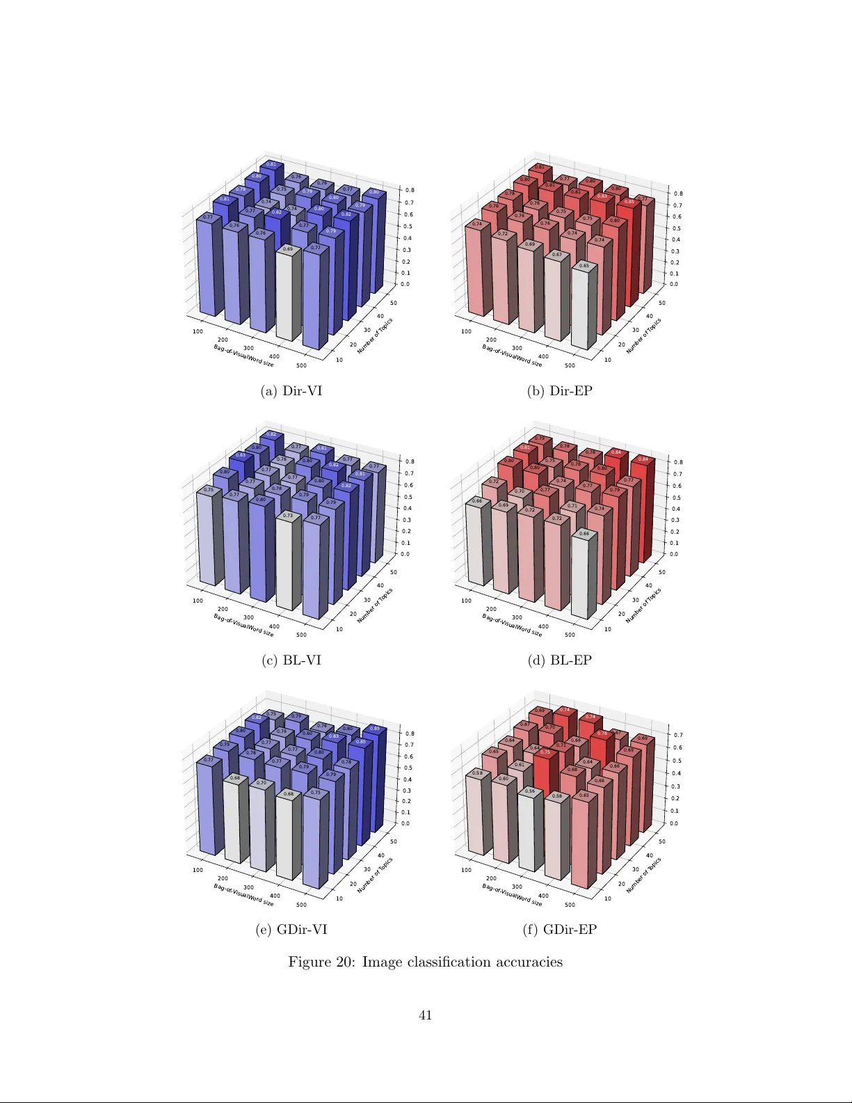
V ectorized Ba y esian Inference for Laten t Diric hlet-T ree Allo cation Zheng W ang zheng.w ang.20211@mail.concordia.ca Conc or dia Institute for Information Systems Engine ering Conc or dia University Montr e al, QC H3G 1M8, Canada Nizar Bouguila nizar.bouguila@concordia.ca Conc or dia Institute for Information Systems Engine ering Conc or dia University Montr e al, QC H3G 1M8, Canada Abstract Laten t Dirichlet Allo cation (LDA) is a foundational mo del for disco vering latent thematic structure in discrete data, but its Diric hlet prior cannot represent the rich correlations and hierarchical relationships often presen t among topics. W e in tro duce the framew ork of Latent Diric hlet-T ree Allo cation (LDT A), a generalization of LDA that replaces the Diric hlet prior with an arbitrary Diric hlet-T ree (DT) distribution. LDT A preserves LDA’s generativ e structure but enables expressiv e, tree-structured priors ov er topic prop ortions. T o perform inference, w e dev elop univ ersal mean-ﬁeld v ariational inference and Exp ectation Propagation, providing tractable up dates for all DT. W e reveal the v ectorized nature of the t wo inference metho ds through theoretical dev elopment, and p erform fully vectorized, GPU-accelerated implementations. The resulting framework substan tially expands the mo deling capacity of LDA while maintaining scalabilit y and computational eﬃciency . The source co de is av ailable at https://gith ub.com/intaiyjw/ldta. Keyw ords: Ba yesian Computing, Laten t Diric hlet Allocation, Diric hlet-T ree, Mean-Field V ariational Inference, Exp ectation Propagation 1 In tro duction Probabilistic topic modeling has b ecome one of the central framew orks for understanding laten t structure in large, unorganized collections of discrete data. As digital text, image annotations, scien tiﬁc literature, biomedical data, and so cial media conten t contin ue to gro w at unprecedented scale, to ols for discov ering hidden themes and in terpretable patterns ha ve b ecome indisp ensable in machine learning and data mining (Blei, 2012). Among these tools, Laten t Diric hlet Allo cation (LDA) has play ed a foundational role. Since its introduction b y Blei et al. (2003), LDA has remained one of the most widely used generative models for unsup ervised learning of thematic structure. Its inﬂuence extends far b eyond text analysis: LD A has b een applied in genetics (Liu et al., 2016), mark eting (Hofmann, 1999), computer vision (F ei-F ei and Perona, 2005), recommendation systems (W ang and Blei, 2011), and man y other domains where observ ed data can b e in terpreted as arising from mixtures of laten t comp onen ts. The original LD A mo del assumes that each do cumen t is represented b y a probability v ector o ver laten t topics, and each topic is a probabilit y distribution o ver a v o cabulary of W ang and Bouguila terms (Blei et al., 2003). Crucially , LDA places a Diric hlet prior ov er the do cumen t-level topic prop ortions. This choice of prior has several attractive prop erties: it is conjugate to the m ultinomial distribution, it facilitates tractable posterior up dates, and it induces a simple geometric in terpretation on the simplex (Bishop, 2006; Gelman et al., 2013). Ho w- ev er, the Diric hlet prior also imp oses structural limitations. Although its parameters can con trol concen tration and sparsity , the Dirichlet distribution cannot express ﬁne-grained correlations among topic comp onents b ey ond the inheren t negative dep endence due to the simplex constrain t (W allac h et al., 2009). As a result, while LDA is simple and eﬀective, it is often too rigid to capture the complex hierarchical or clustered topic structures that arise in real data. This limitation has led to numerous extensions and generalizations of LDA. Correlated T opic Mo dels (Blei and Laﬀerty, 2007) introduced a logistic–normal prior to enco de ric her co v ariance structures, while hierarchical topic mo dels suc h as the Hierarchical Pac hink o Allo cation Model (Li and McCallum, 2006) and the neste d Chinese restauran t pro cess (Blei et al., 2010) allow for topic hierarchies and tree structures. Although these mo dels provide greater ﬂexibility , they t ypically sacriﬁce conjugacy and introduce substantial computa- tional ov erhead. Many suc h models require non-conjugate v ariational inference or sampling pro cedures, which can be computationally exp ensive and diﬃcult to scale (Hoﬀman et al., 2013; T eh et al., 2006). A pow erful y et underutilized alternative to the Dirichlet distribution is the Dirichlet- T ree (DT) distribution, conceptualized for the ﬁrst time by Connor and Mosimann (1969) and later revived in works b y Dennis I II (1991) and Mink a (1999). The Dirichlet-T ree dis- tribution pro vides a natural wa y to enco de structured correlations through a tree of nested Diric hlet random v ariables. Each in ternal no de of the tree deﬁnes a sub-Dirichlet distribu- tion gov erning how probability mass is split among its children, and the full distribution o ver the lea ves (which lie on the simplex) arises from the m ultiplicative combination of these lo cal branching decisions. This form ulation has tw o particularly attractiv e properties: (1) it can express arbitrarily ric h correlation patterns and hierarchical structures b y c ho osing appropriate tree shapes, and (2) it retains man y of the computational con veniences of the ordinary Dirichlet distribution, including lo cal conjugacy and analytical tractability . Giv en the adv an tages of the Dirichlet-T ree distribution, it is natural to ask whether the traditional LD A mo del can b e generalized by replacing the Diric hlet prior with a Dirichlet- T ree prior. Doing so w ould allo w topic mo dels to encode complex prior structures—such as that certain topics should co-o ccur, that some topics form meaningful groups, or that certain topics follow hierarc hical relationships—without abandoning the general framework of LD A. Indeed, the sp ecial cases of Dirichlet-T ree, including Beta-Liouville (Gupta and Ric hards, 1987; Bakh tiari and Bouguila, 2016) and Generalized Dirichlet (F ang et al., 1990; W ong, 1998; Bakhtiari and Bouguila, 2014), hav e b een explored and utilized in recent topic mo deling literature. This idea motiv ates the framework developed in this pap er, which we call Laten t Diric hlet–T ree Allo cation (LDT A). LDT A generalizes LDA by allowing an arbi- trary Dirichlet-T ree to gov ern the topic prop ortions. It preserv es the generative seman tics of LDA, retains in terpretabilit y , and supp orts a broad class of structured priors suitable for mo deling realistic topic correlations. How ever, generalizing LDA to LDT A also introduces signiﬁcan t challenges in p osterior inference. While LDA b eneﬁts from the conjugacy of the Diric hlet and multinomial distributions, LDT A in tro duces a hierarchical and p otentially 2 Vectorized Ba yes for LDT A deep tree structure whose in ternal dep endencies complicate up dates. Eﬃcien t and scalable inference algorithms are therefore essential. Tw o inﬂuential approaches to approximate Ba yesian inference are particularly relev ant: Mean-Field V ariational Inference (MFVI) and Exp ectation Propagation (EP). Mean-Field V ariational Inference (MFVI) (Jordan et al., 1999; W ainwrigh t and Jordan, 2008; Blei et al., 2017), introduced in the late 1990s and no w widely used in mo dern machine learning, replaces the exact p osterior with a factorized approximation c hosen to optimize a low er b ound on the log marginal lik eliho o d (the evidence lo wer b ound, or ELBO). V ari- ational inference is deterministic, often fast, and well-suited for mo dels where conjugacy pro vides closed-form up dates. It has b ecome a standard tool for scalable Bay esian mo del- ing and is used in diverse settings ranging from Ba yesian neural netw orks to probabilistic graphical mo dels. F or LDT A, v ariational inference enables the deriv ation of structured co- ordinate ascent algorithms that up date each factor of the v ariational distribution in closed or semi-closed form. On the other hand, Exp ectation Propagation (EP), in tro duced b y Mink a (2001); Mink a and Laﬀerty (2002), tak es a diﬀerent approac h. Rather than optimizing a low er b ound, EP iterativ ely appro ximates eac h non-conjugate factor in the mo del by pro jecting it onto a c hosen exp onen tial family distribution through momen t matching. EP often pro vides more accurate appro ximations than MFVI, esp ecially in models where the p osterior is not w ell appro ximated b y fully factorized distributions (mean-ﬁeld) (Mink a, 2005). EP has b een used in Gaussian pro cess classiﬁcation (Hern´ andez-Lobato and Hern´ andez-Lobato, 2016), Ba yesian logistic regression (V ehtari et al., 2020), and many other settings where non- conjugacy arises. F or LDT A, EP oﬀers a principled w ay to approximate the in teractions b et w een diﬀeren t nodes of the Dirichlet-tree, yielding improv ed p osterior estimates at the cost of increased algorithmic complexit y . As mo dern machine learning applications frequen tly inv olv e very large corp ora, it is critical that inference algorithms for topic mo dels leverage vectorized computation and GPU acceleration. F rameworks such as PyT orc h (P aszke et al., 2019) hav e made it easy to express complex probabilistic up dates in terms of batched tensor op erations that can run eﬃciently on CUD A-capable GPUs. While traditional implemen tations of LDA rely on nested lo ops and sequen tial up dates, a v ectorized implemen tation can exploit parallelism across documents, topics, and tree no des. Suc h acceleration is essen tial for large datasets where non-vectorized metho ds would b e prohibitively slo w. This pap er dev elops b oth mean-ﬁeld v ariational inference and Exp ectation Propaga- tion algorithms for LDT A and implements them in a fully vectorized fashion that exploits GPU parallelism. The resulting algorithms can p erform eﬃcien t inference ev en for large corp ora and complex Dirichlet-tree structures. Compared with scalar or lo op-based imple- men tations, the v ectorized approac h drastically reduces runtime and allo ws the algorithm to scale to mo dern datasets. The remainder of the paper proceeds as follows. W e develop an impro ved and comprehensive formulation of Dirichlet-T ree in Section 2, revealing the prop erties of Diric hlet-T ree and preparing it to integrate in to LD A, mean-ﬁeld v ariational inference and expectation propagation. In Section 3, we describ e the LDT A mo del, whic h is a generalization of LD A by extending the Dirichlet prior to an arbitrary Dirichlet-T ree distribution. In Section 4, a v ectorized univ ersal mean-ﬁeld v ariational inference metho d is deriv ed for any LDT A mo del. In Section 5, we in terpret the idea and demonstrate the 3 W ang and Bouguila implemen tation steps of the v ectorized Expectation Propagation for an y LDT A mo del. In Section 6, we choose three typical Diric hlet-T ree priors: the conv en tional Dirichlet, the Beta-Liouville and the Generalized Dirichlet to implement our mo dels. W e v alidate and compare our metho ds by a range of exp erimen ts including do cument mo deling, do cumen t and image classiﬁcation, and RNA-sequencing in bioinformatics. Finally , in Section 7, we conclude our pap er and discuss the p oten tial future directions. 2 Diric hlet-T ree This section serves as a formal and comprehensiv e introduction to the Diric hlet-T ree dis- tribution. Diric hlet-T ree was dev elop ed as a generalization of Dirichlet distribution by Dennis I II (1991) and further explored by Mink a (1999). W e further prov e the exp onen tial form of Diric hlet-T ree distribution, and the triple forms of Diric hlet-T ree are concluded: the no de form, the general form and the exp onen tial form. As a result, we show that Dirichlet- T ree remains a conjugate prior to the m ultinomial lik eliho o d with a transformed parameter up dating. Finally , sev eral imp ortan t concepts including Bay esian op erator are prop osed to further assist the deriv ation of v ectorized inferences for Laten t Dirichlet-T ree Allo cation. 2.1 T ree The tree is a well-studied data structure in computer science. It is useful to introduce sev eral tree-related notations before deriving the Diric hlet-T ree distribution. Figure 1 shows a general tree with heigh t v alues of 3. A tree consists of m ultiple no des and branc hes (or edges). W e refer to any node λ that has multiple c hild no des, including the ro ot node, as an in ternal no de; and the set for all in ternal no des is denoted by Λ . In particular, Λ \ r denotes the set of all in ternal no des except the ro ot node. An y node ω that do es not ha ve a c hild no de is called a terminal no de (or leaf ) and the set of all terminal no des is Ω . Bet ween a paren t no de and one of its child nodes is a branc h (or edge). W e use t | s to denote the branc h starting from no de s and p ointing to no de t . An indicator function δ t | s ( ω ) whose domain is Ω is deﬁned and assigned to each branc h: δ t | s ( ω ) =    1 , if the branch t | s leads to leaf ω , 0 , otherwise ω ∈ Ω , s ∈ Λ Sometimes, the starting no de of a branch do es not matter, and w e denote this branch that directly points to no de s as s |∗ . W e deﬁne the function l ( s ) , s ∈ Λ ∪ Ω as the num b er of terminal no des that a no de s trav els to. When s is the ro ot no de, we hav e: l ( r ) = X t | r X ω ∈ Ω δ t | r ( ω ) = K where K = | Ω | is the num b er of all terminal no des. F or s ∈ Ω , we hav e: l ( s ) = X ω ∈ Ω δ s |∗ ( ω ) = 1 , s ∈ Ω 4 Vectorized Ba yes for LDT A F or any s ∈ Λ \ r : l ( s ) = X ω ∈ Ω δ s |∗ ( ω ) = X t | s X ω ∈ Ω δ t | s ( ω ) , s ∈ Λ \ r W e further deﬁne the function c ( s ) , s ∈ Λ as the num b er of direct c hild no des (or branc hes) under an internal no de. F or example, in Figure 1, c ( λ 2 ) = 3. The following theorem is ob vious and useful to mention: Theorem 1 In a tr e e structur e, for any internal no de s ∈ Λ , l ( s ) = c ( s ) + X t | s ( l ( t ) − 1) , s ∈ Λ . (1) Figure 1: Notation for a general tree structure 2.2 Hierarc hical Multinomial and Dirichlet-T ree The Dirichlet distribution has b een widely used as a conjugate prior to multinomial under con ven tional parameterization (Mink a, 1999; Blei et al., 2003; Bishop, 2006). Mink a (1999) describ ed the sample of a con ven tional m ultimomial as the outcome of a K-sided die. In this analogy , a K-sided die is rolled once and one out of K p ossible outcomes is pro duced, where eac h outcome is assigned to a p ossibilit y matter p k , k = 1 , 2 , · · · , K . As in Figure 2 (a), we can formally represent the conv en tional multinomial by assigning eac h p k to a branch in a tree with height 1. The probability mass function (PMF) is given b y: p ( ω | p ) = Y ω | r p ω | r δ ω | r ( ω ) , ω ∈ Ω , p ∈ ∆ K − 1 , r is ro ot 5 W ang and Bouguila (a) (b) (c) Figure 2: (a) Conv entional Multinomial; (b) Hierarc hical Multinomial; (c) Dirichlet-T ree Corresp ondingly , its conjugate Dirichlet can b e represented b y the same tree with eac h branc h assigned a parameter α ω | r , and eac h leaf assigned the comp onent of the ( K − 1)- dimensional simplex. The probability densit y function (PDF) follows: Dir( θ | α r ) = 1 B ( α r ) Y ω ∈ Ω θ ω α ω | r − 1 , θ ∈ ∆ | Ω |− 1 , α r ∈ R K > 0 , r is ro ot B ( α r ) = Q ω | r Γ  α ω | r  Γ  P ω | r α ω | r  where ∆ | Ω |− 1 is the ( | Ω | − 1)-dimensional simplex deﬁned by: ∆ | Ω |− 1 = ( θ ∈ R | Ω |      θ ω ≥ 0 , X ω ∈ Ω θ ω = 1 ) In the case of Diric hlet, | Ω | = K . Despite its conv enience as a conjugate prior for multi- nomial, Diric hlet suﬀers from the following limitations: (i) all comp onen ts share a common v ariance parameter although eac h comp onen t has its o wn mean (Mink a, 1999), and (ii) the co v ariance betw een an y tw o comp onen ts is strictly negativ e (Mosimann, 1962). T o solv e these limitations, Dennis II I (1991) developed the Dirichlet-T ree distribution as a general- ization of Dirichlet. Instead of rolling a K -dimensional die once, the sample of a multinomial can also b e though t of as rolling sev eral diﬀeren t dice for ﬁnite times, as shown in Figure 2 (b). This ﬁnite sto c hastic process results in a hierarc hical multinomial under a tree-lik e parameteri- zation with the following PMF: p ( ω | ρ ) = Y s ∈ Λ Y t | s ρ t | s δ t | s ( ω ) , ω ∈ Ω , ρ s ∈ ∆ c ( s ) − 1 s , s ∈ Λ (2) Consequen tly , the corresp onding prior for the hierarc hical m ultinomial is based on the collection of | Λ | indep enden t Diric hlets endow ed with a tree structure (Figure 2 (c)). And 6 Vectorized Ba yes for LDT A the PDF is given b y: p ( ρ | ξ ) = Y s ∈ Λ 1 B ( ξ s ) Y t | s ρ t | s ξ t | s − 1 , ρ s ∈ ∆ c ( s ) − 1 s , ξ s ∈ R c ( s ) > 0 , s ∈ Λ (3) This is not the ﬁnal form of Dirichlet-T ree distribution yet. What w e w ant is a distribution o ver ( | Ω | − 1)-dimensional simplex assigned to the set of terminal no des. A transformation from ρ ∈ Q s ∈ Λ ∆ c ( s ) − 1 s to θ ∈ ∆ | Ω |− 1 is needed to ac hieve this distribution. As (2) implies, the comp onen t θ ω assigned to a terminal no de is equal to the pro duct of all probabilit y mass assigned to the branches that lead to the terminal no de. W e denote this mapping as follo ws: T : Y s ∈ Λ ∆ c ( s ) − 1 s → ∆ | Ω |− 1 , ρ 7→ T ( ρ ) θ ω = Y s ∈ Λ Y t | s ρ t | s δ t | s ( ω ) , ω ∈ Ω T ( ρ ) =  s ∈ Λ T s ( ρ s ) (4) where T is the comp osition of all sub-mappings T s under eac h in ternal no de. Con v ersely , to show the in verse transform T − 1 , we ﬁrst deﬁne the no de mass Θ s : Θ s ( θ ) =    1 , s is the ro ot , P ω ∈ Ω δ s |∗ ( ω ) θ ω , s ∈ Λ \ r ∪ Ω Ob viously , Θ ω = θ ω when ω ∈ Ω . Thus, we ha ve the inv erse transform as follows: T − 1 : ∆ | Ω |− 1 → Y s ∈ Λ ∆ c ( s ) − 1 s , θ 7→ T − 1 ( θ ) ρ t | s = Θ t Θ s , s ∈ Λ (5) No w, w e ha ve a pair of in verse transforms and assume the transform to b e smo oth. W e go back to (4) and deriv e the Jacobian of T . F or ∀ s ∈ Λ , we denote the sub-transform b y free-co ordinates representation: T s ( ρ s ) : ( ρ 1 | s , . . . , ρ c ( s ) − 1 | s , Θ s ) 7→ (Θ 1 , . . . , Θ c ( s ) ) Note that we enumerate the set of immediate child no des of no de s by 1 , . . . , c ( s ). F or i = 1 , . . . , c ( s ) − 1 and j = 1 , . . . , c ( s ) − 1: ∂ Θ i ∂ ρ j | s = ∂  ρ i | s Θ s  ∂ ρ j | s = Θ s 1 { i = j } , ∂ Θ c ( s ) ∂ ρ j | s = ∂  1 − P c ( s ) − 1 l =1 ρ l | s  Θ s  ∂ ρ j | s = − Θ s F or the column corresp onding to Θ s : ∂ Θ i ∂ Θ s = ρ i | s , i = 1 , . . . , c ( s ) 7 W ang and Bouguila Th us, we ha ve the Jacobian with the form: J T s = Θ s I c ( s ) − 1 b c ⊤ d ! where I c ( s ) − 1 is ( c ( s ) − 1)-dimensional identit y , b = ( ρ 1 | s , . . . , ρ c ( s ) − 1 | s ) ⊤ , c ⊤ = ( − Θ s , . . . , − Θ s ), d = ρ c ( s ) | s . Th us, the determinan t derives as follows: det( J T s ) = det(Θ s I c ( s ) − 1 )  d − c ⊤  Θ s I c ( s ) − 1  − 1 b  = Θ s c ( s ) − 1 (6) According to the change-of-v ariable theorem, what we call the no de form of Dirichlet-T ree is derived as follo ws by com bining (3), (5) and (6): DT( θ | ξ ) = p  T − 1 ( θ ) | ξ  | det( J T ) | − 1 = Y s ∈ Λ 1 B ( ξ s )  1 Θ s  c ( s ) − 1 Y t | s  Θ t Θ s  ξ t | s − 1 , θ ∈ ∆ | Ω |− 1 , ξ ∈ R P s ∈ Λ c ( s ) > 0 (7) It is easy to derive a more general form of Dirichlet-T ree from (7). Based on this general form, we give a formal deﬁnition of Diric hlet-T ree distribution. Deﬁnition 2 (General form of Diric hlet-T ree) With r esp e ct to a tr e e structur e wher e r is the r o ot no de, Ω is the set of terminal no des and Λ \ r is the set of the r emaining no des, a Dirichlet-T r e e distribution is a pr ob ability me asur e on ∆ | Ω |− 1 with PDF DT( θ | ξ ) = 1 B ( ξ r ) Y ω ∈ Ω θ ω ξ ω |∗ − 1   Y s ∈ Λ \ r 1 B ( ξ s ) Θ s ξ s |∗ − ξ ∗| s   (8) wher e ξ t | s ∈ R > 0 is assigne d to e ach br anch for s ∈ Λ , and ξ ∗| s = X t | s ξ t | s and B ( · ) is the multivariate b eta function. 2.3 Exp onen tial F orm and Conjugacy W e further pro ve that a Dirichlet-T ree distribution b elongs to the exp onen tial family . The exp onen tial form of a Diric hlet-T ree is given as follows: Theorem 3 (Exp onen tial form of Diric hlet-T ree) DT( θ | ξ ) = Y s ∈ Λ 1 B ( ξ s ) Y t | s  Θ t Θ s  ξ t | s − l ( t ) = exp   X s ∈ Λ X t | s  ξ t | s − l ( t )  log  Θ t Θ s  − log Y s ∈ Λ B ( ξ s )   (9) wher e l ( t ) is the numb er of le af no des that the no de t le ads to. 8 Vectorized Ba yes for LDT A Pro of Dividing (7) by (9) yields Y s ∈ Λ  1 Θ s  c ( s ) − 1 Y t | s  Θ t Θ s  l ( t ) − 1 = Y s ∈ Λ  1 Θ s  c ( s )+ P t | s ( l ( t ) − 1) − 1 !   Y t ∈ Λ \ r ∪ Ω Θ l ( t ) − 1 t   = Y s ∈ Λ  1 Θ s  l ( s ) − 1 !   Y t ∈ Λ \ r Θ l ( t ) − 1 t   = 1 The deriv ation uses Theorem 1 and the fact that Θ root = 1 The natural parameter, suﬃcient statistics, normalizer, and base measure are resp ectively denoted as: η t | s ( ξ ) = ξ t | s − l ( t ) , s ∈ Λ u t | s ( θ ) = log  Θ t Θ s  , s ∈ Λ g ( η ( ξ )) = Y s ∈ Λ B ( ξ s ) h ( θ ) = 1 Giv en the e xponential form, all properties of the exp onen tial family listed in App endix A will apply . Corollary 4 (Exp ectation of suﬃcien t statistics) E DT( θ | ξ )  log  Θ t Θ s  = ∂  log Q s ∈ Ω B ( ξ s )  ∂ ξ t | s = ψ  ξ t | s  − ψ  ξ ∗| s  , s ∈ Λ ξ ∗| s = X t | s ξ t | s W e pro ceed to sho w the conjugacy of Diric hlet-T ree to an y con ven tional | Ω | -dimensional m ultinomial. Com bining the pair of the transforms (4) and (5), we can represent eac h comp onen t θ ω assigned to a terminal node b y node mass and indicator functions assigned to non-terminal no des and branches as follows: θ ω = Y s ∈ Λ Y t | s  Θ t Θ s  δ t | s ( ω ) , ω ∈ Ω (10) 9 W ang and Bouguila Let a Diric hlet-T ree distribution with Ω b e the prior to a | Ω | -dimensional multinomial. Giv en a collection of multinomial samples n = ( n 1 , . . . , n K ) where K = | Ω | , the posterior is given as: p ( θ | n ) ∝ p ( n | θ ) p ( θ ) ∝ Y ω ∈ Ω θ ω n ω !   Y s ∈ Λ Y t | s  Θ t Θ s  ξ t | s − l ( t )   = exp    X ω ∈ Ω n ω log θ ω + X s ∈ Λ X t | s  ξ t | s − l ( t )  log  Θ t Θ s     = exp    X ω ∈ Ω n ω X s ∈ Λ X t | s δ t | s ( ω ) log  Θ t Θ s  + X s ∈ Λ X t | s  ξ t | s − l ( t )  log  Θ t Θ s     = exp    X s ∈ Λ X t | s ξ t | s + X ω ∈ Ω n ω δ t | s ( ω ) − l ( t ) ! log  Θ t Θ s     No w it is obvious that the p osterior remains the same kind of Diric hlet-T ree with a trans- formed parameter up dating. F or conv enience, we denote the p osterior Dirichlet-T ree as DT( θ | ξ ′ ) = DT( θ | ξ ⊕ p n ) = DT( θ | ξ + D p n ) where w e call ⊕ p the Ba yesian addition; and D p the Diric hlet selection op erator as D p selects the comp onen ts from the partitioned samples to add to the Dirichlet-T ree parameter corresp onding to eac h branch in the tree structure; and ξ t | s ′ = ξ t | s + X ω ∈ Ω n ω δ t | s ( ω ) , s ∈ Λ W e hav e the follo wing corollary b y combining Corollary 4 and (10): Corollary 5 (Log-space exp ectation) E DT( θ | ξ ) [log θ ω ] = E DT( θ | ξ )   X s ∈ Λ X t | s δ t | s ( ω ) log  Θ t Θ s    = X s ∈ Λ X t | s δ t | s ( ω )  ψ ( ξ t | s ) − ψ ( ξ ∗| s )  In tuitively , the exp ectation of log θ ω is equal to the sum of E DT( θ | ξ )  u t | s  corresp onding to all the branches that leads to ω . 2.4 Ba yesian operator In this section, w e prop ose several concepts based on the exp onen tial form and conjugacy of Dirichlet-T ree to further assist the deriv ations of tw o approximate Bay esian inference algorithms in tro duced in the following sections. In the Ba yesian inference of generative 10 Vectorized Ba yes for LDT A graphical models lik e Laten t Diric hlet Allocation (Blei et al., 2003), it is common to ha ve a substantial n um b er of parameter up dating pro cesses. Ba yesian operator is prop osed to represen t this kind of processes in a compact w ay . W e ﬁrst give the formal deﬁnition of Ba yesian op erator: Deﬁnition 6 (Ba yesian op erator) L et T b e the statistic al manifold of Dirichlet-T r e e. In c onjugacy to multinomial, the Bayesian op er ator for ∀ p ∈ T tr ansforms the p as a prior to a p osterior p ′ ∈ T given the multinomial observation n : p ′ = B ( n ) p It is easy to deriv e: B ( n ) =  g ( η ( ξ + D p n )) g ( η ( ξ ))  − 1 exp  n ⊤ log θ  The Ba yesian op erator exhibits a closure nature and pro vides a new expression of conjugacy . The mathematical expression in our follo wing deriv ation of Exp ectation Propagation is largely simpliﬁed with the Ba y esian op erator. Given the Ba y esian op erator, the relationship b et w een the Dirichlet selection op erator and the Bay esian op erator is built, whic h is our cen tral theorem: Theorem 7 (The cen tral theorem) p ( θ | ξ + D p n ) = B ( n ) p ( θ | ξ ) Ev en though the m ultinomial observ ation n is non-negative integers, n can b e naturally extended to any real n umbers in Ba yesian operator that mak es the posterior meaningful. The Bay esian op erator satisﬁed the following prop erties: • Additivit y and Commutativit y B ( n 1 + n 2 ) = B ( n 1 ) B ( n 2 ) = B ( n 2 ) B ( n 1 ) Pro of RHS =  g ( η ( ξ + D p ( n 1 + n 2 ))) g ( η ( ξ ))  − 1 exp  ( n 2 + n 1 ) ⊤ log θ  = LHS • In verse operator B − 1 ( n ) = B ( − n ) • Base p osteriors F or ∀ p ( θ | ξ ) ∈ T , there exists a group of base p osteriors { p ( θ | ξ + D p 1 ( k ) ) } K : p ( θ | ξ + D p 1 ( k ) ) = B ( 1 ( k ) ) p ( θ | ξ ) , k = 1 , . . . , K where K = | Ω | and 1 ( k ) is the K -dimensional binary v ector where k th elemen t equals 1 and 0 otherwise. W e also use p ( θ | ξ + D p 1 ( k ) ) to represent the group of derived distributions { p ( θ | ξ + D p 1 ( k ) ) } K . 11 W ang and Bouguila Corollary 8 (Exp ectation op erator) E p ( θ | ξ ) " K Y k =1 θ k n k # = Z ∆ K − 1 exp  n ⊤ log θ  p ( θ | ξ ) d θ = Z ∆ K − 1  g ( η ( ξ + D p n )) g ( η ( ξ )) B ( n )  p ( θ | ξ ) d θ = g ( η ( ξ + D p n )) g ( η ( ξ )) Z ∆ K − 1 p ( θ | ξ + D p n ) d θ = g ( η ( ξ + D p n )) g ( η ( ξ )) = Y s ∈ Λ B ( ξ s + D p n ) B ( ξ s ) = Y s ∈ Λ   Q t | s Γ  ξ t | s ′  Γ  P t | s ξ t | s ′      Γ  P t | s ξ t | s  Q t | s Γ  ξ t | s    = Y s ∈ Λ Γ  P t | s ξ t | s  Γ  P t | s ξ t | s + P t | s P ω ∈ Ω n ω δ t | s ( ω )  Y t | s Γ  ξ t | s + P ω ∈ Ω n ω δ t | s ( ω )  Γ  ξ t | s  In p articular, E p ( θ | ξ ) [ θ k ] = g ( η ( ξ + D p 1 ( k ) )) g ( η ( ξ )) = Y s ∈ Λ Γ  P t | s ξ t | s  Γ  P t | s ξ t | s + P t | s P ω ∈ Ω 1 ( k ) δ t | s ( ω )  Y t | s Γ  ξ t | s + P ω ∈ Ω 1 ( k ) δ t | s ( ω )  Γ  ξ t | s  = Y s ∈ Λ Γ  P t | s ξ t | s  Γ  P t | s ξ t | s + P t | s δ t | s ( k )  Y t | s Γ  ξ t | s + δ t | s ( k )  Γ  ξ t | s  ! = Y s ∈ Λ 1 P t | s ξ t | s ! P t | s δ t | s ( k ) Y t | s ξ t | s δ t | s ( k ) , k = 1 , . . . , K ; s ∈ Λ The deriv ation of the corollary uses the Gamma function’s prop ert y: Γ( x + 1) = x Γ( x ) In tuitively , the exp ectation of eac h comp onent θ k of Diric hlet-T ree is equal to the pro duct of parameter prop ortions corresp onding to all branches that lead to the comp onen t. 12 Vectorized Ba yes for LDT A 2.5 Deriv ed Distributions of Dirichlet-T ree It is useful to deﬁne the group of deriv ed distributions to assist the Bay esian inference in the following sections. Deﬁnition 9 (Deriv ed distributions of Dirichlet-T ree) L et p ( θ | ξ ) ∈ T b e a Dirichlet- T r e e. The c orr esp onding gr oup of derive d distributions { p t | s ( θ ) } | Λ | is deﬁne d as: p t | s ( θ ) = E p ( θ | ξ )  u t | s ( θ )  − 1 u t | s ( θ ) p ( θ | ξ ) , s ∈ Λ F or notational simplicity , and when no ambiguit y arises, we replace the label t | s for each branc h with d , and | Λ | = D . W e also denote | Ω | = K . Corollary 10 (Exp ectation matrix of deriv ed distributions) By stacking the exp e c- tation of e ach derive d distribution, the ( K × D )-dimensional exp e ctation matrix is derive d, and e ach c olumn gives: E p d ( θ ) [ θ ] =  Z ∆ K − 1  g ( η ( ξ + D p 1 ( k ) )) g ( η ( ξ )) B ( 1 ( k ) )  E p ( θ | ξ ) [ u d ( θ )] − 1 u d ( θ ) p ( θ | ξ ) d θ  K k =1 =  g ( η ( ξ + D p 1 ( k ) )) g ( η ( ξ )) E p ( θ | ξ ) [ u d ( θ )] − 1 Z ∆ K − 1 u d ( θ ) p ( θ | ξ + D p 1 ( k ) ) d θ  K k =1 = E p ( θ | ξ ) [ θ ] ⊙ k E p ( θ | ξ + D p 1 ( k ) ) [ u d ( θ )] E p ( θ | ξ ) [ u d ( θ )] , d = 1 , . . . , D (11) wher e D = | Λ | and ⊙ k is the Hadamar d (element-wise) pr o duct with r esp e ct to the subscript k . 3 Laten t Diric hlet-T ree Allo cation In this section, we introduce Laten t Diric hlet-T ree Allo cation (LDT A), whic h generalizes the Latent Dirichlet Allo cation mo del of Blei et al. (2003) b y replacing the Diric hlet prior with an arbitrary Dirichlet-T ree. Similar to LDA, LDT A is a generativ e probabilistic graph- ical model. F or clarit y , we adopt column-ma jor order in the mathematical formulation of the mo del, whereas the implemen tation uses ro w-ma jor order to adhere to standard pro- gramming conv en tions. 3.1 The Generativ e Pro cess Tw o sets with known cardinalities V and K are p ostulated b efore constructing our mo del: (i) the collection of V words (the vocabulary , or visual w ords in the case of images): W = { w 1 , . . . , w v , . . . , w V } and (ii) the collection of K topics: Z = { z 1 , . . . , z k , . . . , z K } 13 W ang and Bouguila The observed data set is a sequence of M do cumen ts (the corpus, or images): D = ( w 1 , . . . , w m , . . . , w M ) where each do cumen t is a sequence of N m w ords: w m = ( w 1 m , . . . , w nm , . . . , w N m m ) , w nm ∈ W In LDT A, a latent topic is assumed with resp ect to eac h observed w ord: z m = ( z 1 m , . . . , z nm , . . . , z N m m ) , z nm ∈ Z Sometimes, w e ignore the subscript m to simply keep our notation uncluttered when we refer to any document in D . According to the ex-changeabilit y assumption (Blei et al., 2003), we only care ab out the o ccurring num b ers of the words that app eared in a do cumen t, instead of the order of the word sequence. Therefore, we indicate eac h w ord as a binary vector 1 ( v ) nm ∈ { 0 , 1 } V deﬁned ov er W , where the v th elemen t equals 1 if the v th w ord is c hosen, and 0 otherwise. Consequently , w e obtain the word counting vector of a do cument by summing up all the word indicator vector: n m = ( n 1 m , . . . , n v m , . . . n V m ) ⊤ = N m X i =1 1 ( v ) im T aking the latent topics in to accoun t, the binary indicator vector for eac h word is lifted to a binary matrix 1 ( v k ) nm ∈ { 0 , 1 } V × K , deﬁned ov er W × Z , to represent word–topic co-o ccurrence. Similarly , w e obtain the w ord–topic coun ting matrix for a do cumen t b y summing up all the w ord–topic indicator matrices: n m = { n v k } ( V × K ) =         n 11 · · · n 1 k · · · n 1 K . . . . . . . . . n v 1 · · · n v k · · · n v K . . . . . . . . . n V 1 · · · n V k · · · n V K         = N m X i =1 1 ( v k ) im Moreo ver, the do cumen t–w ord–topic counting tensor is constructed by stacking counting matrices of all do cumen ts in the data set (Figure 3). Similar to LDA, LDT A is probabilistic graphic mo del. The generativ e pro cess for each do cumen t is describ ed as follows: 1. Draw N ∼ P oisson( µ ). 2. Draw θ ∼ DT( ξ ). 3. F or each w ord w n for n = 1 , . . . , N : (a) Draw z n ∼ Mult( θ ). (b) Draw w n ∼ Mult( φ z n ). 14 Vectorized Ba yes for LDT A Figure 3: The do cumen t–topic–word coun ting tensor. And the whole generation pro cess pro duced our data set by rep eating ab ov e pro cedures for M times (Figure 4). Among the parameters, ξ is the hyper-parameter for the Dirichlet- T ree prior; θ ∈ ∆ K − 1 is the topic proportion with resp ect to Z , and w e denote the square diagonal form of each do cumen t’s prop ortion as M ( θ m ); φ is a word–topic conditional probabilit y matrix deﬁned as the conditional probability of generating v th w ord giv en the k th topic: φ = { φ v k } V × K =         φ 11 · · · φ 1 k · · · φ 1 K . . . . . . . . . φ v 1 · · · φ v k · · · φ v K . . . . . . . . . φ V 1 · · · φ V k · · · φ V K         and w e assume φ to b e non-generated. By m ultiplying the w ord–topic conditional probabil- it y matrix and the square diagonal form of each do cumen t’s topic prop ortion, we obtain the join t probability matrix of the co-o ccurrence of eac h word–topic couple in each do cumen t: Φ m =         φ 11 θ 1 · · · φ 1 k θ k · · · φ 1 K θ K . . . . . . . . . φ v 1 θ 1 · · · φ v k θ k · · · φ v K θ K . . . . . . . . . φ V 1 θ 1 · · · φ V k θ k · · · φ V K θ K         = φ M ( θ ) The relationship of the v ariables in LDT A expressed in tensors is sho wn in Figure 5. 3.2 The Join t and the Marginalized Distributions Giv en the hyper-parameters ξ and φ , as w ell as the conditional indep endence assumption of the v ariables, the joint distribution of the laten t parameters and the observ ed coun ting v ector for a single do cumen t is giv en by: p ( w , z , θ | φ , ξ ) = p ( w | z , φ ) p ( z | θ ) p ( θ | ξ ) = p ( θ | ξ ) N m Y n =1 p ( z n | θ ) p ( w n | z n , φ ) 15 W ang and Bouguila Figure 4: Graphical representation (plate notation) of LDT A mo del. The shaded circle rep- resen ts the observed v ariable; the blank circles represen t the latent v ariables and diamonds indicate hyper-parameters. The arrows imply dep enden t generativ e relationship and the rectangles with num b er at its right-lo w er corner represen t rep etitions. Figure 5: T ensor expression of relationship of the v ariables where w and z are sequences of words and topics resp ectively . Based on ab ov e discussion, the order of the w ord sequence is trivial and can simply b e replaced by counting matrix 16 Vectorized Ba yes for LDT A { n v k } ( V × K ) . Hence, each term is resp ectively represen ted as: p ( θ | ξ ) = DT( θ | ξ ) p ( z | θ ) = K Y k =1 θ k n k = K Y k =1 V Y v =1 θ k n vk p ( w | z , φ ) = K Y k =1 V Y v =1 φ v k n vk Therefore, we arrive at the pro duct form of prior m ultiplying likelihoo d: p ( w , z , θ | φ , ξ ) = DT( θ | ξ ) K Y k =1 V Y v =1 ( φ v k θ k ) n vk By collapsing the topic sequence, we deriv e the joint distribution of observ ed w and latent θ : p ( w , θ | φ , ξ ) = X z p ( w , z , θ | φ , ξ ) = DT( θ | ξ ) V Y v =1 X { n vk } K  n v n v 1 , · · · , n v k , · · · , n v K  K Y k =1 ( φ v k θ k ) n vk = DT( θ | ξ ) V Y v =1 K X k =1 φ v k θ k ! n v It is noteworth y to men tion that a document’s probabilit y vector o v er word collection W denoted as { t v ( θ ) = P K k =1 φ v k θ k } V is determined given the do cument-topic prop ortion v ector θ and topic-word conditional probability matrix φ : { t v ( θ ) } V v =1 =         φ 11 · · · φ 1 k · · · φ 1 K . . . . . . . . . φ v 1 · · · φ v k · · · φ v K . . . . . . . . . φ V 1 · · · φ V k · · · φ V K                 θ 1 . . . θ k . . . θ K         = K X k =1 φ 1 k θ k , . . . , K X k =1 φ v k θ k , . . . , K X k =1 φ V k θ k ! ⊤ By in tegrating out the latent v ariable θ , the evidence, or the marginal distribution of observ ed word coun ting vector is given: p ( w | φ , ξ ) = Z ∆ K − 1 p ( w , θ | φ , ξ )d θ = Z ∆ K − 1 DT( θ | ξ ) V Y v =1 ( t v ( θ )) n v d θ 17 W ang and Bouguila Finally , we compute the total probabilit y of corpus D containing M do cumen ts: p ( D | φ , ξ ) = M Y m =1 p m ( w m | φ , ξ ) = M Y m =1 Z θ m DT( θ m | ξ ) V Y v =1 ( t v m ( θ m )) n vm d θ m 4 Mean-Field V ariational Inference The mean-ﬁeld v ariational inference emplo ys a global mean-ﬁeld distribution to p erform appro ximation for eac h latent no de in the probabilistic graph. The approximated p osterior is achiev ed b y minimizing the KL-divergence: q ( z | η ∗ ) = arg min q ∈Q KL( q ( z | η ) || p ( z | w )) = arg min q ∈Q Z z q ( z | η ) log q ( z | η ) p ( z | w ) d z whic h is equiv alent to maximizing Evidence Low er Bound (ELBO): ELBO = Z z q ( z | η ) log p ( w , z ) q ( z | η ) d z Since we will deal with b oth con tinuous v ariables (topic proportions) and discrete v ariables (topics) in our mo del, we in tro duce a new notation: D f ( x ) , g ( x ) E x =    P i f ( x i ) g ( x i ) , if x is discrete , R x f ( x ) g ( x ) d x, if x is contin uous The feasibility of v ariational mean-ﬁeld as an appro ximating distribution lies on the inde- p endency assumption b etw een its random v ariables, whic h leads to an imp ortan t prop ert y: D y ( x n ) , q ( x 1 ) q ( x 2 ) · · · q ( x n ) · · · q ( x N ) E x = D y ( x n ) , q ( x n ) E x n This enables us to expand the joint distribution o ver every individual laten t or observ ed v ariable node in the generativ e probabilistic graph, and deal with each ELBO term with resp ect to the corresp onding latent nodes separately from an external viewp oin t. By taking the probabilistic graph in Figure 4 as demonstrating example, we illustrate the deriv ation of mean-ﬁeld v ariational inference and provide a general algorithm regardless of the speciﬁc Diric hlet-T ree prior. More inference algorithms for the generalized probabilistic graphs can b e easily deriv ed in a similar manner. 4.1 The Evidence Lo wer Bound Supp ose p ( θ | ξ ) is a Dirichlet-T ree distribution with selection matrix D p and p ( θ | ξ ) is em- plo yed as the prior distribution in the generativ e plate notation in Figure 4. W e already 18 Vectorized Ba yes for LDT A pro ve that p ( θ | ξ ) is b oth a member of exp onen tial family and a conjugate prior to the m ultinomial: p ( θ | ξ ) = exp { η ( ξ ) T u ( θ ) − log g ( η ( ξ )) } Without the need to sp ecify the concrete expression, the univ ersal form of appro ximation al- gorithm and k ey steps in the optimization is demonstrated by only utilizing Diric hlet-T ree’s prop erties of exp onential family and conjugacy to Multinomial. Our goal is to approximate the join t p osterior distribution p ( z , θ | w , φ , ξ ) of all latent v ariables of interest given the observ ed sequences w , and the global mean-ﬁeld approximating distribution is deﬁned as: q ( θ , z | ζ , ϕ ) = M Y m =1 q ( θ | ζ m ) N m Y n =1 q ( z nm | ϕ nm ) It is ob vious that the global appro ximation wip es out the original dependency b et ween v ari- ables such as the dep endency b et ween θ and z . Given the approximating distribution, the optimized parameters are obtained b y minimizing KL( q ( θ , z | ζ , ϕ ) || p ( θ , z | w , φ , ξ )), whic h is equiv alen t to maximizing the Evidence Low er Bound (ELBO): L ( ζ , ϕ ; ξ , φ ) =  log p ( w , z , θ | ξ , φ ) q ( z , θ | ζ , ϕ ) , q ( z , θ | ζ , ϕ )  ( z , θ ) = M X m =1  D log p ( θ | ξ ) E q ( θ | ζ m ) + D log p ( z | θ ) E q ( θ | ζ m ) q ( z | ϕ m ) + D log p ( w m | z , φ ) E q ( z | ϕ m ) − D log q ( θ | ζ m ) E q ( θ | ζ m ) − D log q ( z | ϕ m ) E q ( z | ϕ m )  = M X m =1  D log p ( θ m | ξ ) E q ( θ m | ζ m ) + N m X n =1 D log p ( z nm | θ m ) E q ( θ m | ζ m ) q ( z nm | ϕ nm ) + N m X n =1 D log p ( w nm | z nm , φ ) E q ( z nm | ϕ nm ) − D log q ( θ m | ζ m ) E q ( θ m | ζ m ) − N m X n =1 D log q ( z nm | ϕ nm ) E q ( z nm | ϕ nm )  19 W ang and Bouguila Without loss of generalit y , w e consider ELBO for an y one of the do cuments and drop the subscript m . W e hav e: L m ( ζ , ϕ ; ξ , φ ) = η ( ξ ) T E q ( θ | ζ ) [ u ( θ )] − log g ( η ( ξ )) + N X n =1 ϕ n T E q ( θ | ζ ) [log θ ] + N X n =1 ϕ n T log φ v ( n ) − η ( ζ ) T E q ( θ | ζ ) [ u ( θ )] + log g ( η ( ζ )) − N X n =1 ϕ n T log ϕ n = " η ( ξ ) − η ( ζ ) + D q N X n =1 ϕ n !# T E q ( θ | ζ ) [ u ( θ )] + log g ( η ( ζ )) − log g ( η ( ξ )) + N X n =1 ϕ n T log φ v ( n ) − N X n =1 ϕ n T log ϕ n where the subscript v indicates the v th c hoice from the dictionary at the n th observ ed w ord, and D q represen ts Dirichlet selection matrix which dep ends only on the structure of appro ximator q ( θ | ζ ) regardless of the v alue of ζ . The tensor expression of ELBO is shown in Figure 6. It is notew orthy to men tion that the form of this sp eciﬁc expression of ELBO dep ends only on the sp eciﬁc generative probabilistic graph with the corresp onding no des replaced by the c hoice of the sp eciﬁc Diric hlet-T ree distribution. 4.2 E-Step • Optimization in terms of ζ P arameter ζ belongs to q ( θ | ζ ) ov er a do cument’s topic prop ortion θ , one term of the global appro ximating mean-ﬁeld. W e diﬀerentiate the ELBO with resp ect to ζ : ∇ ζ L ( ζ ) = ∇ ζ    " η ( ξ ) − η ( ζ ) + D q N X n =1 ϕ n !# T E q ( θ | ζ ) [ u ( θ )] + log g ( η ( ζ )) + C    = " ξ − ζ + D q N X n =1 ϕ n !# T ∇ ζ E q ( θ | ζ ) [ u ( θ )] =    " ξ − ζ + D q N X n =1 ϕ n !# T  ∂ ∂ ζ d E q ( θ | ζ ) [ u ( θ )]     D d =1 20 Vectorized Ba yes for LDT A Figure 6: T ensor expression of ELBO Figure 7: Exp ectation-Maximization iteration pro cess of mean-ﬁeld v ariational inference By setting deriv atives to 0 , w e hav e: ζ ∗ = ξ + D q N X n =1 ϕ n ! = ξ ⊕ q N X n =1 ϕ n ! 21 W ang and Bouguila Notice that ϕ n only depends on the observed w ords w v in this single document, the opti- mization step can b e expressed in terms of matrix multiplication: ζ ∗ = ξ ⊕ q { ϕ kv n v } K • Optimization in terms of ϕ P arameter ϕ is matrix { ϕ kn } ( K × N ) , the m ultinomial parameters of Q N n =1 q ( z n | ϕ n ) given the observ ed word w n at eac h lo cation n . The optimized ϕ ∗ is obtained b y maximizing the ELBO, whic h is a constrained optimization problem with resp ect to ϕ where there are N constrain ts: K X l =1 ϕ ln = 1 , n = 1 , 2 , · · · , N Without loss of generality , we consider the Lagrangian function with resp ect to ϕ kn of ϕ n : L ( ϕ n ) = ϕ n T E q ( θ | ζ ) [log θ ] + ϕ n T log φ v ( n ) − ϕ n T log ϕ n + N X n =1 λ n K X l =1 ϕ ln − 1 ! + C ∂ L ∂ ϕ kn = E q ( θ | ζ ) [log θ k ] + log φ v k − log ϕ kn − 1 + λ n By setting partial deriv atives with resp ect to ϕ nk zero, we hav e: ϕ kn ∗ = φ v k exp  E q ( θ | ζ ) [log θ k ] + λ n − 1  where exp { λ n − 1 } is the normalizer. Since { ϕ n } N dep ends only on whic h word { w v n } N out of v o cabulary { w v } V is chosen, the matrix { ϕ kn } ( K × N ) is transformed in to { ϕ kv } ( K × V ) for Q V v =1 q ( z | ϕ v ) n v , where n v is the coun t of the v th w ord in the document. Therefore, the optimization step can b e expressed in terms of matrices: { ϕ kv } ∗ ( K × V ) =  z v − 1 φ v k exp  E q ( θ | ζ ) [log θ k ]  ( K × V ) = n z v − 1 φ v k exp  D T q  E q ( θ | ζ ) [ u ( θ )]  k o ( K × V ) where z v is the normalizer. The E-step of mean-ﬁeld v ariational inference is concluded in Algorithm 1. 4.3 M-Step Giv en optimized { q ( θ | ζ ∗ m ) } M and { ϕ ∗ kv m } ( K × V × M ) after an inference step, w e pro ceed to optimize the mo del’s h yp er-parameters ξ and { φ v k } V × K b y maximizing ELBO on all do c- umen ts D : L ( ξ , φ ) = M X m =1 ( η ( ξ ) T E q ( θ | ζ ∗ m ) [ u ( θ )] − log g ( η ( ξ )) + N m X n =1 ϕ ∗ nm T log φ v ( nm ) ) + C 22 Vectorized Ba yes for LDT A Algorithm 1: V ariational mean-ﬁeld inference for a single do cumen t w m Input: Prior ξ , { φ v k } V × K ; Observ ation coun t { n v } V Output: Optimized ζ , { ϕ kv } K × V Initialize each element in { ϕ kv } K × V as 1 /K ; Initialize ζ = ξ ⊕ { ϕ kv n v } K ; while not c onver genc e do for w v in W in p ar al lel do Compute { ϕ kv } new ( K × V ) =  φ v k exp { E q ( θ | ζ ) [log θ k ] }  ( K × V ) ; Normalize { ϕ kv } new ( K × V ) suc h that P K k =1 ϕ kv = 1; Up date ζ new = ξ ⊕ { ϕ new kv n v } K ; • Optimization of φ ELBO with resp ect to φ is giv en as: L ( φ ) = M X m =1 N m X n =1 ϕ ∗ nm T log φ v ( nm ) + C Notice that φ has K constraints: V X l =1 φ lk = 1 , k = 1 , 2 , · · · , K and the Lagrangian is giv en as: L ( φ ) = M X m =1 N X n =1 ϕ ∗ nm T log φ v ( nm ) + K X k =1 λ k V X v =1 φ v k − 1 ! = V X v =1 K X k =1 M X m =1 ϕ ∗ kv m n v m ! log φ v k + K X k =1 λ k V X v =1 φ v k − 1 ! Without loss of generality , the partial deriv atives of Lagrangian with resp ect to φ v k is written as: ∂ L ∂ φ v k = M X m =1 ϕ ∗ kv m n v m ! 1 φ v k + λ k By setting the partial deriv atives to zero, we hav e: φ v k ∗ = − 1 λ k M X m =1 ϕ ∗ kv m n v m ! Therefore, the optimized { φ v k } ∗ ( V × K ) is derived as: { φ v k } ∗ ( V × K ) = ( z k − 1 M X m =1 ϕ ∗ kv m n v m ) ( V × K ) 23 W ang and Bouguila where { z k } K is the normalizer. • Optimization of ξ ELBO with resp ect to ξ is given as: L ( ξ ) = η ( ξ ) T M X m =1 E q ( θ | ζ ∗ m ) [ u ( θ )] ! − M log g ( η ( ξ )) + C The ﬁrst-order deriv ative is written as: ∇ ξ L ( ξ ) = ( M X m =1 E q ( θ | ζ m ) [ u d ( θ )] − M E p ( θ | ξ ) [ u d ( θ )] ) D d =1 By setting the deriv ative to zero, we can see that the optimized ξ is obtained by matching the moment of hyper-Dirichlet with parameter ξ to the av erage of those of the inferred p osteriors, whic h is a similar pro cess to the message passing in Exp ectation Propagation. Th us, we pro ceed with Newton’s metho d, and the Hessian is derived as: H ξ L ( ξ ) = − M  ∂ ∂ ξ i E p ( θ | ξ ) [ u j ( θ )]  ( D × D ) The optimized ξ ∗ can b e appro ximated iteratively b y Newton’s metho d: ξ ( t +1) := ξ ( t ) − H ( ξ ( t ) ) − 1 ∇ ( ξ ( t ) ) The tensor expression of the whole Exp ectation-Maximization is shown in Figure 7. 5 Exp ectation Propagation In Ba yesian inference, we compute the p osterior distribution on laten t v ariables giv en the observ ation. In mean-ﬁeld v ariational inference, the algorithm employs a global mean-ﬁeld distribution to perform approximation for eac h latent node in the probabilistic graph. In con trast, Exp ectation Propagation (EP) separates target distributions into terms, appro x- imate each one and com bine together to obtain a global appro ximation. 5.1 F ormal Alignmen t of Approximate Distribution to T arget Posterior In EP for LDT A, w e fo cus on the marginal p osterior on θ giv en the observed sequence of w ords incorp orating the mo del’s hyper-parameters. F or a single do cumen t w e ha ve the target marginal p osterior: p ( θ | w , φ , ξ ) = p ( w , θ | φ , ξ ) p ( w | φ , ξ ) ∝ p ( θ | ξ ) V Y v =1 K X k =1 φ v k θ k ! n v = p ( θ | ξ ) exp D n v , log t v ( θ ; φ ) E v 24 Vectorized Ba yes for LDT A where t v ( θ ; φ ) = K X k =1 φ v k θ k W e can see that the hierarc hical probabilistic graph leads to the transform of lik eliho o d breaking the conjugacy , where the comp ound of θ and φ makes it imp ossible to revise the parameters directly from prior, and ev entually causes the whole p osterior to b e intractable. Therefore, w e need to employ appro ximating metho ds suc h as V ariational Inference or Exp ectation Propagation with tractable distributions to estimate the in tractable target p osterior. The mean-ﬁeld v ariational inference is introduced in the last section, and we demonstrate the Exp ectation Propagation routine in the following. • Dual conjugate expressions In EP , w e try to appro ximate the target distribution b y an approximating distribution with the similar form: q ( θ ) ∝ p ( θ | ξ ) exp D n v , log ˜ t v ( θ ) E v In con trast to v ariational mean-ﬁeld where we simply optimize the approximating distri- bution’s parameter by maximizing the ELBO, EP p erforms a more in-depth ﬁne-grained calibration based on the structure of target distribution b y constraining the functional space of the appro ximating distributions. In addition to the requirements of tractablility suc h as pre-normalization and independence that v ariational mean-ﬁeld complies, EP fur- ther exp ects the pro duction form of the approximating distribution, in accordance with the prior-likelihoo d-p oin ts product form of the target distribution. Moreov er, due to the nature of lik eliho o d, the observ ation n ( v ) is incorp orated in to the appro ximator, whic h in eﬀect imposes a constrain t on the functional space of the appro ximating distribution. Giv en the bijectiv e corresp ondence of the terms betw een the appro ximator and the target, dis- tributed term-to-term appro ximation is achiev ed by momen t matc hing in a serial or parallel manner, while the simplicity of global normalization is main tained. Based on the further requiremen ts on appro ximator in EP , Diric hlet-T ree with the same selection matrix D as the prior’s is c hosen as the approximator of target posterior, thanks to its dual conjugate expressions: q ( θ | ζ n ) = q ( θ | ξ + D q n ( k ) ) = B q ( n ( k ) ) p ( θ | ξ ) = (  g ( η ( ζ n )) g ( η ( ξ ))  − 1 exp D n k , log θ k E k ) p ( θ | ξ ) ∝ p ( θ | ξ ) exp D n k , log θ k E k where D q is Diric hlet selection matrix and B q the Ba yesian op erator. W e call the ﬁrst expression whose parameters are directly revised the explicit form of approximator, and the second expression conforming the target the implicit form of approximator. It is notew orthy to men tion that the global normalizer is determined if laten t { n k } K on the set of topic is giv en. 25 W ang and Bouguila • Explicitization of pseudo-observ ation Ev en though it closely resem bles the target distribution, the inner pro duct expression for the lik eliho o d terms is with resp ect to the topic dimension k which relies on the latent v ariable z , instead of the word dimension v in those of the target distribution which is dra wn directly from the observed w . T o contin ue constructing our appro ximate distribution, w e introduce the transition matrix { ϕ kv } ( K × V ) , which leads to the counting matrix of pseudo-observ ation { ϕ kv n v } ( K × V ) , so that the vector { ϕ kv n v } K appro ximates to { n k } K . Observ ation transition matrix ϕ can roughly be viewed as the pseudo-proportions of k th topic in the authentic count of v th w ord in a do cumen t, therefore the normalization is required. And we call the rev erse transform pro cedure { ϕ kv n v } ( K × V ) , whic h formulates an explicit counting matrix representing both the observed and the latent v ariables, the explicitization of pseudo-observ ation on latent v ariable—in our case the latent topics as direct results of the sto chastic pro cedure sub ject to the multinomial whose parameters are dominated b y the Diric hlet-T ree prior. W e say “pseudo” b ecause the rev erse transform do es not strictly reﬂect the genuine in teger counts as describ ed in our mo del, but gives the decimal estimations instead. Therefore, we ha ve: q ( θ | ζ n ) ∝ p ( θ | ξ ) exp  X v ϕ kv n v , log θ k  k = p ( θ | ξ ) exp X v n v D ϕ kv , log θ k E k = p ( θ | ξ ) exp D n v ,  ϕ kv , log θ k  k E v = p ( θ | ξ ) exp  n v , log Y k θ k ϕ kv  v It is easy to tell that the explicitization of pseudo-observ ation is the process of reversely transforming from the authentic observed v ariable to some appro ximated laten t v ariables, whic h are usually the unseen results of random pro cess controlled by the parameters of in terest, so that the information from authentic observ ation can b e passed to an ob ject whic h helps build a tractable explicit appro ximate posterior on those parameters of in terest. As desired by the inference, the resulted appro ximate p osterior remains a similar implicit pro duct form in compliance with the target prior-lik eliho od-p oints p osterior. W e call the ob ject the pseudo-observ ation. • T erm-wise sync hronization No w, we hav e a quite similar form to the target distribution with t ( θ ; φ ) replaced by Q k θ k ϕ kv . According to Jensen’s inequality: K Y k =1 θ k ϕ kv = exp ( K X k =1 ϕ kv log θ k ) ≤ K X k =1 ϕ kv θ k 26 Vectorized Ba yes for LDT A where P K k =1 ϕ kv = 1. Ho wev er, we hav e: 0 ≤ K X k =1 φ v k ≤ K It is likely that the corresp onding approximate term will b e smaller than the target term— the bigger the topic cardinality K is, the more likely Q k θ k ϕ kv will b e smaller than t ( θ ; φ ). T o solve this inheren t limitation, we add a co eﬃcien t for eac h approximate term to synchro- nize with the target term, whic h will b e remo ved b y global normalizer later. As a result, w e obtain our ﬁnal form of appro ximating likelihoo d terms: ˜ t v ( θ ; ϕ ) = s v K Y k =1 θ k ϕ kv where s v is the sync hronization coeﬃcient such that each ˜ t v ( θ ) approximates t v ( θ ). With eac h appro ximating term obtained, w e deriv e our ﬁnal approximating distribution expres- sions: q ( θ | ζ n ) = q ( θ | ξ + D q ϕn ( v ) ) = B q ( ϕn ( v ) ) p ( θ | ξ ) =  g ( η ( ζ n )) g ( η ( ξ )) exp D n v , log s v E v  − 1 p ( θ | ξ ) exp  n v , log s v K Y k =1 θ k ϕ kv  v ∝ p ( θ | ξ ) exp D n v , log ˜ t v ( θ ; ϕ ) E v No w, it is clear that the transition matrix { ϕ kv } K × V w orks as a transformer whic h con- v erts the observ ation o ver v o cabulary to pseudo-observ ation o ver laten t topics to achiev e a conjugate posterior on the latent v ariable of interest, and to build a series of cell likeli- ho ods in compliance with the likelihoo d of observ ations conforming the target p osterior as a whole without the loss of global normalization. Given the transition matrix { ϕ kv } K × V , observ ation n ( v ) , and hyper-parameter ξ , the parameter ζ n for the explicit appro ximating distribution is given as follows: ζ n = ξ ⊕ ϕn ( v ) It is ob vious to tell that the implicit form of approximate distribution is now in alignment with the target posterior whic h holds a prior-lik eliho o d-points pro duct form. The pro cess of ac hieving this bijectively corresp onding alignmen t from approximate distribution to the target p osterior is called the alignmen t of appro ximate distribution. Figure 8 illustrates the whole picture ov er the relationships among the target p osterior, the explicit approximate distribution, and implicit approximate distribution. 5.2 Ca vity and Tilted Distributions Giv en the explicit and implicit expression of the appro ximating distribution, the appro xima- tor’s statistical manifold is ﬁxed and the task no w is to determine an optimized group of the 27 W ang and Bouguila Figure 8: Construction of appro ximate posterior distribution and its relationship with other parameters. The ( n v ) V and ( n k ) K represen ts observ ed count vector of words, and laten t coun t vector of topics, resp ectiv ely . In explicit p osterior distribution, the normalizer, or the evidence s ( ξ , φ ) is in tractable, which is the reason why w e hav e to use approximate metho d. Notice Q k θ k P v ϕ kv n v = Q v  Q k θ k ϕ kv  n v . ξ ′ is the revision of prior parameter ξ whic h incorp orates the latent coun t of topics ( n k ) K based on the prop ert y of conjugacy . param ter ( ϕ ∗ , s ( v ) ∗ ) as the ﬁnal approximation to target p osterior. With the term-to-term bijectiv e correspondence betw een the appro ximating distribution and the target p osterior, the problem of global approximation is transformed in to the approximation of each term ˜ t v ( θ ; ϕ ) to t v ( θ ; φ ) individually . A series of ca vity and tilted distributions, { q ( θ | ζ \ v ) } V and { p ∗ v ( θ ) } V with respect to eac h term t v ( θ ; φ ) or ˜ t v ( θ ; ϕ ) are built to p erform the pro ceeding appro ximations in a distributed manner. Theoretically , for an ideal approximator q ( θ | ζ ∗ ) where { ˜ t v ( θ ; ϕ ∗ ) = t v ( θ ; φ ) } V , it would cause no eﬀect if an y ˜ t v ( θ ; ϕ ∗ ) is devided out and replaced by t v ( θ ; ϕ ). Ho w ever, for an y initialized v alue ϕ (0) , the statemen t will not hold in general, meaning that the resulted new distributions are neither normalized nor proportional to the original appro ximator. The key of EP is that, due to the nature of the approximating distribution w e choose, a group of normalized distributions { p ∗ v ( θ ) } V with resp ect to ev ery individual term, whic h we call the titled distributions, can b e formulated by unloading the appro ximate term and loading the target term, so that one lo cal individual term is separated and fo cused on eac h time and further optimizations can b e p erformed with resp ect to each term iterativ ely . Suppose w e ha ve the appro ximator q ( θ | ζ ( t ) ) in an iteration. Normalized as they are, the corresp ond- ing { p ∗ ( t ) v ( θ ) } V are not prop ortional to q ( θ | ζ ( t ) ) b ecause there is still a distance b et ween q ( θ | ζ ( t ) ) and target p ( θ | n ( v ) , φ , ξ ). Besides, the tilted distributions con taining informa- 28 Vectorized Ba yes for LDT A Figure 9: EP inference in each iteration. The statistical manifold is conceptually illustrated with three dimensions. The target, the appro ximator and the tilted distributions are all lo cated on the statistical Riemann manifold thanks to the tractabilit y of the appro ximating distribution we c ho ose. The approximator is dra wn to the target by the group of tilted distributions in each iteration. tion from b oth t v ( θ ; φ ) and q ( θ | ζ ( t ) ) lo cate b et w een the target and curren t appro ximator. Starting from the “imp erfect” initial appro ximator q ( θ | ζ (0) ), the approximator is drawn closer to its titled distributions in each iteration, and therefore is dra wn closer to the target p osterior, until the iteration conv erges when q ( θ | ζ ∗ ), { p ∗ v ( θ ) } V , and p ( θ | n ( v ) , φ , ξ ) almost o verlap (Figure 9). The up date of the approximator is further elab orated as follows. In one iteration, supp ose we hav e the transition matrix ϕ ( t ) , and the ca vity distributions { q ( θ | ζ \ v ) } V pla ying the role as a group of background distributions which are formulated as: q ( θ | ζ \ v ) = B − 1 ( ϕ v ) B ( ϕn ( v ) ) p ( θ | ξ ) Notice that the ca vity distributions are naturally normalized due to tractability of approx- imating distribution. Subsequently , the normalized tilted distributions are derived as: p ∗ v ( θ ) = z v − 1 K X k =1 φ v k θ k ! q ( θ | ζ \ v ) where the normalizer { z v } V is trivial to compute: z v = Z θ K X k =1 φ v k θ k ! q ( θ | ζ \ v )d θ = φ v T E q ( θ | ζ \ v ) [ θ ] The messages from the target term contained in the titled distributions are subsequen tly passed to a group of new separate appro ximators, which are of same selection matrix D q as the current appro ximator, by minimizing the KL-divergence: ζ sep v := arg min ζ sep v KL( p ∗ v ( θ ) || q ( θ | ζ sep v )) (12) This pro cess is equiv alent to matc h the moment of tw o distributions and will b e introduced in the next section. After obtaining the optimized { ζ sep v } V , the parameter ϕ is updated 29 W ang and Bouguila suc h that: q ( θ | ζ sep v ) = B ( ϕ ( t +1) v ) q ( θ | ζ \ v ) = q ( θ | ζ \ v + D q ϕ ( t +1) v ) and ϕ ( t +1) v := D − 1 q  ζ sep v − ζ \ v  where D − 1 q is the inv erse selection op erator. In practice, we only fo cus on the leaf no des of D q to obtain the up dated ϕ ( t +1) . The optimization of synchronization coeﬃcient { s v } V is the next step. Supp ose we ha ve ϕ ( t ) in an iteration, and so w e hav e the appro ximate distribution (regardless of explicit or implicit form): q ( θ | ζ ( t ) ) = B ( ϕ ( t ) n ( v ) ) p ( θ | ξ ). Ideally , if q ( θ | ζ ( t ) ) approximates target p osterior enough, the follo wing equation of the corresp onding tilted distributions should hold: q ∗ ( t ) v ( θ ) ≡ q ( θ | ζ ( t ) ) s v K Y k =1 θ ϕ ( t ) kv k ! − 1 K X k =1 φ v k θ k ! = B − 1 ( ϕ v ) B ( ϕn ( v ) ) p ( θ | ξ ) K X k =1 φ v k θ k ! g ( η ( ζ \ v )) g ( η ( ζ )) s v − 1 ≈ B − 1 ( ϕ v ) B ( ϕn ( v ) ) p ( θ | ξ ) K X k =1 φ v k θ k ! z v − 1 where v = 1 , 2 , · · · , V . Consequen tly , we obtain the up date of { s v } V : s v ( t ) := g ( η ( ζ \ v ( t ) )) g ( η ( ζ ( t ) )) z v ( t ) According to the ab ov e discussion, the parameter up date as preparation for message passing in eac h iteration is concluded as Algorithm 2. The whole inference pro cedure for a single do cumen t is concluded as Algorithm 3. The relationship b et w een appro ximator, target, cavit y and tilted distributions is illustrated in Figure 10. 5.3 P arallel Message Passing This section elab orates in detail the pro cess of message passing, whic h is implemented b y momen t matc hing as indicated in (12). The purp ose of message passing is to pass the information of target terms { t v ( θ ; φ ) } V from the tilted distributions { p ∗ v ( θ ) } V to a group of separate approximators { q ( θ | ζ sep v ) } V resp ectiv ely , so that the up dated ϕ ( t +1) can subsequen tly b e obtained by { q ( θ | ζ sep v ) } V p eeling oﬀ the bac kgroud { q ( θ | ζ \ v ) } V to supp ort the newer approximation { ˜ t v ( θ ; ϕ ( t +1) ) } V to { t v ( θ ; φ ) } V . The moment matching is ac hieved in parallel with resp ect to index v . According to Theorem 13 in App endix A, the optimized separate approximators { q ( θ | ζ sep v ) } V deﬁned in (12) are the ones whose exp ectations on suﬃcient statistics equal to those exp ec- tations of the titled distributions. In other words, the optimization pro cess of { q ( θ | ζ sep v ) } V is equiv alen t to matching the moment of { q ( θ | ζ sep v ) } V to { p ∗ v ( θ ) } V . This parallel opti- mization pro cess can be expressed as follows. On the one hand, thanks to the prop ert y of 30 Vectorized Ba yes for LDT A Figure 10: Relationships of Cavit y and Tilted distributions exp onen tial family , the exp ectations on suﬃcien t statistics of separate appro ximators are easily derived, which span a ( D × V ) matrix Q ( ζ sep ) with unknowns ζ sep : Q =         E q sep 1 [ u 1 ( θ )] · · · E q sep v [ u 1 ( θ )] · · · E q sep V [ u 1 ( θ )] . . . . . . . . . E q sep 1 [ u d ( θ )] · · · E q sep v [ u d ( θ )] · · · E q sep V [ u d ( θ )] . . . . . . . . . E q sep 1 [ u D ( θ )] · · · E q sep v [ u D ( θ )] · · · E q sep V [ u D ( θ )]         On the other hand, the ( D × V )-dimensional exp ectation matrix P ( ϕ ( t ) ) on the same group of suﬃcient statistics with resp ect to the tilted distributions { p ∗ v ( θ ) } V is formulated as: P =         E p ∗ 1 [ u 1 ( θ )] · · · E p ∗ v [ u 1 ( θ )] · · · E p ∗ V [ u 1 ( θ )] . . . . . . . . . E p ∗ 1 [ u d ( θ )] · · · E p ∗ v [ u d ( θ )] · · · E p ∗ V [ u d ( θ )] . . . . . . . . . E p ∗ 1 [ u D ( θ )] · · · E p ∗ v [ u D ( θ )] · · · E p ∗ V [ u D ( θ )]         31 W ang and Bouguila Therefore, the moment matching is more sp eciﬁcally expressed b y solving a system of ( D × V ) non-linear equations: Q  ζ sep  ϕ ( t +1)  := P  ϕ ( t )  (13) This system of equations can b e more explicitly reduced to sev eral sub-groups of equations with resp ect to the internal no des of the tree structure in the follo wing form: ψ  ζ t | s  − ψ   X t | s ζ t | s   = C t | s , s ∈ Λ where { ζ t | s } is the sub-group of c hild nodes of no de s and C t | s the constan t from P . Each in- dividual sub-group of equations can b e solv ed n umerically b y ﬁx-point iteration or Newton’s metho d. Notice that P is determined giv en ϕ ( t ) of current iteration: E p ∗ v [ u d ( θ )] = Z θ u d ( θ ) z v K X k =1 φ v k θ k ! q ( θ | ζ \ v )d θ = E q ( θ | ζ \ v ) [ u d ( θ )] z v Z θ K X k =1 φ v k θ k ! 1 E q ( θ | ζ \ v ) [ u d ( θ )] u d ( θ ) q ( θ | ζ \ v )d θ = E q ( θ | ζ \ v ) [ u d ( θ )] φ v T E q d ( θ | ζ \ v ) [ θ ] φ v T E q ( θ | ζ \ v ) [ θ ] = φ v T  E q ( θ | ζ \ v ) [ θ ] ⊙ k E q ( θ | ζ \ v + D q 1 ( k ) ) [ u d ( θ )]  φ v T E q ( θ | ζ \ v ) [ θ ] =  φ v ⊙ k E q ( θ | ζ \ v ) [ θ ]  T E q ( θ | ζ \ v + D q 1 ( k ) ) [ u d ( θ )]  φ v ⊙ k E q ( θ | ζ \ v ) [ θ ]  T 1 (14) The (14) uses the result from (11), where { q ( θ | ζ \ v + D q 1 ( k ) ) } ( K × V ) is the group of base p osteriors of { q ( θ | ζ \ v ) } V . W e can see that the right-hand side of the non-linear equations is reduced to quite a concise and elegan t closed-form solution, meaning that the moment of a tilted distribution equals to the w eighted av erage of the counterparts of its corresp onding ca vity distribution’s base posteriors, where the w eights are given b y the Hadamard pro duct of φ and { E q ( θ | ζ \ v ) [ θ ] } ( V × K ) . 5.4 P arameter Estimation W e em b edded the EP as the E-step in to Expectation-Maximization framework. The opti- mized mo del parameters ξ and { φ v k } V × K measured by Kullback–Leibler divergence are esti- 32 Vectorized Ba yes for LDT A Algorithm 2: Essential parameters up date Input: Prior ξ , { φ v k } V × K ; Observ ation { n v } V ; { ϕ kv } K × V of current iteration Output: ζ ; { ζ \ v } V , { z v } V and { s v } V ; evidence p ( w m ) of current iteration Compute ζ = ξ ⊕ ϕ m n m ; for w v in W in p ar al lel do Compute ζ \ v = ζ ⊖ ϕ v ; Compute z v = φ v T E q ( θ | ζ \ v ) [ θ ]; Compute s v = z v g ( η ( ζ \ v )) /g ( η ( ζ )); Compute p ( w m ) = exp ⟨ n v , log s v ⟩ v g ( η ( ζ )) /g ( η ( ξ )); Algorithm 3: EP inference for a single do cumen t w m Input: Prior ξ , { φ v k } V × K ; Observ ation coun t { n v } V Output: Optimized { ϕ kv ∗ } ( K × V ) , { s v ∗ } V ; Estimated evidence p ( w m ) Initialize each element in { ϕ kv } K × V as 1 /K ; Initialize essential parameters as Algorithm 2; while not c onver genc e do for w v in W in p ar al lel do Compute ζ sep v b y moment matc hing as Algorithm 4; Compute ϕ ( t +1) v = ζ sep v ⊖ ζ \ v ; Normalize ϕ ( t +1) v suc h that P k ϕ kv = 1; Up date essential parameters as Algorithm 2; Algorithm 4: Moment matching Input: Essen tial parameters obtained in Algorithm 2 Output: Optimized separate approximators { ζ sep v } V for w v in W in p ar al lel do Compute E q ( θ | ζ \ v ) [ θ ]; for d = 1 to D in p ar al lel do for k = 1 to K in p ar al lel do Compute E q ( θ | ζ \ v + D q 1 ( k ) ) [ u d ( θ )]; Compute E p ∗ v [ u d ( θ )] according to (14); Compute { ζ sep v } V b y Newton’s metho d according to (13); 33 W ang and Bouguila Figure 11: T ensor expression of Exp ectation Propagation mated b y maximizing the Evidence Lo w er Bound (ELBO) with respect to ξ and { φ v k } V × K : L ( ξ , φ ) = M X m =1 E q ( θ | ζ m ) [log p ( θ | ξ )] + M X m =1 E q ( θ | ζ m ) [log p ( w m | φ , θ )] + C = M X m =1 ( η ( ξ ) T E q ( θ | ζ m ) [ u ( θ )] − log g ( η ( ξ )) + E q ( θ | ζ m ) " V X v =1 n v m log K X k =1 φ v k θ k !#) + C (15) The optimization is p erformed ov er the collection of all do cuments D . The whole learning algorithm is depicted in Algorithm 5, and the tensor expression is shown in Figure 11. 6 Exp erimen ts In this section, w e test and ev aluate LDT A with three diﬀerent kinds of Diric hlet-T ree priors: the Dirichlet, the Beta-Liouville and the generalized Dirichlet. The details of these three distributions are listed in App endix C. Both t wo inference metho ds are examined in three problem domains: do cument mo deling, document and image classiﬁcation, and a bioinformatics task. Our exp erimen ts are p erformed on several publicly a v ailable and well- kno wn datasets: NIPS, Reuters-21578, 20 Newsgroups, 15 Scene Categories and P erpheral Blo od Mononuclear Cells (PBMC). 34 Vectorized Ba yes for LDT A Algorithm 5: EP-embedded EM algorithm Input: Do cumen t collection D Output: Appro ximated distribution parameters { ϕ kv m } K × V × M , { s v m } V × M , estimated evidence { ˆ p ( w m ) } M ; Mo del parameters φ , ξ Initialize φ , ξ ; while not c onver genc e do // EP-Inference for w m in D do Giv en mo del parameters, approximate the p osterior by EP as Algorithm 3; // Maximization Giv en the appro ximated p osteriors, optimize mo del parameters according to (15) 6.1 Do cumen t mo deling Dataset In do cumen t modeling, we fo cus on NIPS dataset, whic h contains a corpus of 1740 research articles accepted by Neural Information Pro cessing Systems conference from 1987-2016. Prepro cessing As a necessary prepro cessing procedure for raw documents, w e ﬁrst to- k enize the do cumen ts and remov e num b ers, punctuations, and stop words suc h as those with less than tw o letters. Next, all words are reduced to their ro ot form b y a standard lemmatizer from NL TK library . T o capture more sp eciﬁc and iden tiﬁable seman tic ob jects, bigrams are additionally recognized and added to the token list. Finally , we remov e the w ords that are to o rare or to o common and generate the vocabulary . Mo dels and experiment description After prepro cessing and tokenizing the ra w do c- umen ts, w e train a series of topic mo dels with diﬀerent model settings: (i) three typical Diric hlet-T ree priors: original Dirichlet, Beta-Lioville and Generalized Dirichlet; (ii) t wo v ectorized inference metho ds: Mean-Field V ariational Inference and Exp ectation Propaga- tion; and (iii) a range of topic quantities from 10, 20, to 80. Therefore, in total, w e train and examine 3 × 2 × 8 = 48 diﬀerent topic mo dels. W e ev aluate the obtained mo dels by metrics including (i) conv ergence of log-lik eliho o d, (ii) predictiv e p erplexit y , (iii) topic coherence and (iv) topic div ersity . 6.1.1 Convergence The ELBO v alues are computed and recorded in eac h training iteration for all mo dels. Equally for all model settings, the training pro cess is judged as con verged when the ELBO’s c hange rate is less than 1e-4. Fig. 12 shows the ELBO v alues with resp ect to each iteration in diﬀeren t mo dels. W e can see that the training pro cess of all mo dels conv erges successfully after several iterations. The mo dels with v ariationl inference generally ac hieves a little adv antage in ﬁnal ELBO v alues, while the mo dels with exp ectation propagation conv erges in less iterations. 35 W ang and Bouguila 6.1.2 Predictive perplexity P erplexity measures the quality of a topic mo del b y ev aluating its predictiv e capability on hold-out test set. W e split the dataset in to 90% training set and 10% test set to chec k the mo dels’ predictiv e p erplexity . W e ﬁrst train a mo del on the training set, and then p erform inference on the test set. In practice, the p erplexit y in our exp erimen t is computed as follo ws: P erplexity( D test ) = exp ( − P M m =1 P V v =1 n mv log P K k =1 φ v k E q m ( ζ ) [ θ k ] P M m =1 P V v =1 n mv ) Fig. 13 plots the p erplexit y of diﬀerent mo del settings. 6.1.3 Topic Coherence and Diversity T opic coherence and topic diversit y are tw o complemen tary metrics to measure the quality of learned topics. T opic coherence targets at eac h individual topic and ev aluate the seman tic similarity within the top words assigned to a topic. Popular topic coherence measures include UCI Coherence, UMass Coherence, and CV Coherence. In our exp erimen ts, we use a mixing topic coherence measure provided by Gensim library . T op ten words are chosen for eac h topic, and one model’s coherence v alue is computed by a veraging the coherence v alues of eac h topic. On the contrary , topic diversit y measures how “orthogonal”, or dissimilar the generated topics are against each other. A go od model should hav e diverse topics to con vey abundan t information dimensions. In practice, our topic diversit y is computed as follo ws: Div ersity( φ ) = U ( N ) K N where K is the n um b er of topics, N is n umber of top words chosen for each topic, and U is n umber of unique words within these top w ords. W e c ho ose N = 10 for our exp eriments. Fig. 14 and Fig. 15 shows the results of topic coherence and topic div ersity , rep ectiv ely . W e observ e that V ariational Inference generally has b etter topic coherence, while exp ectation propagation has b etter topic diversit y . 6.2 Do cumen t Classiﬁcation In the tasks of document classiﬁcation, a collection of documents are categorized in to binary or multiple classes, where each do cumen t is represen ted b y a ﬁxed set of features (Blei 2003). A natural thinking is to use the counts of all the words that appear in a do cumen t as the represen tative features, y et leading to an extremely large feature space. T opic models pla y the role of dimension reduction in do cumen t classiﬁcation, where the large vocabulary is reduced to K-dimensional simplex. In our exp erimen t, we use Reuters-21578 corpus set whic h is a collection of lab eled newswire articles. After necessary prepro cessing, we choose the six categories that contain the most do cumen ts. Finally , w e obtain a vocabulary of 4562 unique words, and 7460 do cumen ts in total. The num b ers of do cumen ts in eac h category are shown in T able 1. 36 Vectorized Ba yes for LDT A 0 4 8 12 16 20 24 28 32 Iteration 1.85 1.80 1.75 1.70 1.65 1.60 1.55 ELB O 1e7 K=10 K=20 K=30 K=40 K=50 (a) Dir-VI 0 3 6 9 12 15 18 21 Iteration 1.85 1.80 1.75 1.70 1.65 1.60 ELB O 1e7 K=10 K=20 K=30 K=40 K=50 (b) Dir-EP 0 4 8 12 16 20 24 28 Iteration 1.85 1.80 1.75 1.70 1.65 1.60 1.55 ELB O 1e7 K=10 K=20 K=30 K=40 K=50 (c) BL-VI 0 2 4 6 8 10 12 14 16 18 Iteration 1.85 1.80 1.75 1.70 1.65 1.60 ELB O 1e7 K=10 K=20 K=30 K=40 K=50 (d) BL-EP 0 4 8 12 16 20 24 28 32 36 Iteration 1.85 1.80 1.75 1.70 1.65 1.60 1.55 ELB O 1e7 K=10 K=20 K=30 K=40 K=50 (e) GDir-VI 0 2 4 6 8 10 12 14 Iteration 1.85 1.80 1.75 1.70 1.65 1.60 ELB O 1e7 K=10 K=20 K=30 K=40 K=50 (f ) GDir-EP Figure 12: ELBO con v ergence with resp ect to iterations; iterations stop when ELBO c hange less than 0.0001 37 W ang and Bouguila 10 20 30 40 50 60 70 80 Number of T opics 2200 2400 2600 2800 3000 3200 3400 3600 P erple xity Dir - VI Dir -EP BL - VI BL -EP GDir - VI GDir -EP Figure 13: Perplexit y 10 20 30 40 50 60 70 80 Number of T opics 0.425 0.450 0.475 0.500 0.525 0.550 0.575 0.600 0.625 T opic Coher ence Dir - VI Dir -EP BL - VI BL -EP GDir - VI GDir -EP Figure 14: T opic Coherence 10 20 30 40 50 60 70 80 Number of T opics 0.60 0.65 0.70 0.75 0.80 0.85 0.90 0.95 1.00 T opic Diversity Dir - VI Dir -EP BL - VI BL -EP GDir - VI GDir -EP Figure 15: T opic Diversit y 10 20 30 40 50 Number of T opics 0.88 0.89 0.90 0.91 0.92 0.93 0.94 0.95 0.96 A verage accuracy VI EP Figure 16: Average classiﬁcation accuracy of Dirichlet prior 10 20 30 40 50 Number of T opics 0.88 0.89 0.90 0.91 0.92 0.93 0.94 0.95 0.96 A verage accuracy VI EP Figure 17: Average classiﬁcation accuracy of Beta-Liouville prior 10 20 30 40 50 Number of T opics 0.800 0.825 0.850 0.875 0.900 0.925 0.950 A verage accuracy VI EP Figure 18: Average classiﬁcation accuracy of Generalized Dirichlet prior 38 Vectorized Ba yes for LDT A T able 1: Number of do cuments of chosen categories Category # Do cuments earn 3900 acq 2289 crude 370 trade 324 money-fx 306 in terest 271 W e train multiple m odels with diﬀerent settings for the whole corpus, and compute the exp ectation of each do cumen t’s p osterior distribution as its representativ e feature. Subse- quen tly , w e train a logistic regression classiﬁer based on the learned topic prop ortions and the original lab els. F or each topic mo del setting, we randomly split the corpus into 80% training set and 20% test set for 10 times. The a verage classiﬁcation accuracy , as w ell as its standard deviation, is computed and employ ed as its ﬁnal accuracy result. Figure 16, Figure 17 and Figure 18 are, resp ectiv ely , the results of classiﬁcation accuracy of Dirichlet prior, Beta Liouville prior, and Generalized Dirichlet prior. T able 2 shows the sp eciﬁc accuracy v alue of each mo del setting. F or each mo del setting, w e c ho ose the topic n umber that generates the highest av erage accuracy and demonstrate its confusion matrix in Figure 19. Mo dels Accuracy K=10 K=20 K=30 K=40 K=50 Dir-VI 92.0% 93.2% 94.4% 95.6% 94.6% Dir-EP 88.6% 91.6% 91.8% 93.5% 93.9% BL-VI 93.3% 92.7% 94.9% 95.3% 95.0% BL-EP 88.9% 92.3% 92.4% 92.5% 92.6% GDir-VI 79.9% 94.2% 95.1% 93.9% 93.8% GDir-EP 84.1% 86.8% 91.3% 91.6% 90.5% T able 2: Average accuracy of classiﬁcation 6.3 Image Classiﬁcation W e further examine our mo dels with an image classiﬁcation task. W e choose 15 Scene Categories dataset, and pick ﬁve categories out of them: forest, highw ay , kitc hen, oﬃce, and tallbuilding. After loading the ﬁv e categories of images, their feature descriptors are extracted with SIFT(Scale-In v arian t F eature T ransform), which are roughly distributed in a contin uous space. Thus, w e use K-MEANS on all obtained descriptors to form bag-of-visualword (BoVW) v o cabulary . Then, a topic mo del with a certain prior-inference com bination is trained on the BoVM, and the topic prop ortions of each image are obtained. Subsequently , 39 W ang and Bouguila acq crude ear n inter est money -fx trade P r edicted label acq crude ear n inter est money -fx trade T rue label 0.97 0.00 0.02 0.00 0.00 0.00 0.01 0.95 0.03 0.00 0.01 0.00 0.02 0.00 0.98 0.00 0.00 0.00 0.04 0.00 0.00 0.83 0.13 0.00 0.00 0.00 0.03 0.18 0.75 0.03 0.00 0.02 0.02 0.00 0.08 0.89 K=40 0.0 0.2 0.4 0.6 0.8 (a) Dir-VI acq crude ear n inter est money -fx trade P r edicted label acq crude ear n inter est money -fx trade T rue label 0.98 0.00 0.02 0.00 0.00 0.00 0.11 0.84 0.04 0.00 0.00 0.01 0.03 0.00 0.97 0.00 0.00 0.00 0.09 0.00 0.04 0.76 0.11 0.00 0.03 0.00 0.05 0.07 0.77 0.08 0.00 0.00 0.11 0.00 0.05 0.85 K=50 0.0 0.2 0.4 0.6 0.8 (b) Dir-EP acq crude ear n inter est money -fx trade P r edicted label acq crude ear n inter est money -fx trade T rue label 0.97 0.01 0.02 0.00 0.00 0.00 0.08 0.88 0.01 0.00 0.00 0.03 0.02 0.00 0.98 0.00 0.00 0.00 0.04 0.00 0.00 0.87 0.09 0.00 0.02 0.00 0.02 0.15 0.77 0.05 0.03 0.00 0.00 0.00 0.05 0.92 K=40 0.0 0.2 0.4 0.6 0.8 (c) BL-VI acq crude ear n inter est money -fx trade P r edicted label acq crude ear n inter est money -fx trade T rue label 0.99 0.00 0.01 0.00 0.00 0.00 0.15 0.80 0.03 0.00 0.00 0.03 0.04 0.00 0.96 0.00 0.00 0.00 0.17 0.00 0.02 0.76 0.06 0.00 0.11 0.00 0.07 0.05 0.74 0.03 0.06 0.00 0.12 0.00 0.02 0.80 K=50 0.0 0.2 0.4 0.6 0.8 (d) BL-EP acq crude ear n inter est money -fx trade P r edicted label acq crude ear n inter est money -fx trade T rue label 0.98 0.00 0.02 0.00 0.00 0.00 0.01 0.91 0.04 0.00 0.01 0.03 0.02 0.00 0.98 0.00 0.00 0.00 0.00 0.00 0.04 0.80 0.15 0.02 0.00 0.02 0.03 0.13 0.79 0.03 0.00 0.00 0.00 0.00 0.06 0.94 K=30 0.0 0.2 0.4 0.6 0.8 (e) GDir-VI acq crude ear n inter est money -fx trade P r edicted label acq crude ear n inter est money -fx trade T rue label 0.94 0.00 0.05 0.00 0.00 0.01 0.09 0.86 0.00 0.00 0.01 0.03 0.04 0.00 0.95 0.00 0.00 0.01 0.04 0.02 0.06 0.70 0.13 0.06 0.07 0.00 0.02 0.00 0.69 0.23 0.00 0.02 0.06 0.00 0.03 0.89 K=40 0.0 0.2 0.4 0.6 0.8 (f ) GDir-EP Figure 19: Best confusion matrix for each mo del settings; the titles indicating the topic n umber 40 Vectorized Ba yes for LDT A 100 200 300 400 500 Bag- of - V isualW or d size 10 20 30 40 50 Number of T opics 0.0 0.1 0.2 0.3 0.4 0.5 0.6 0.7 0.8 0.77 0.76 0.76 0.69 0.77 0.81 0.77 0.82 0.77 0.79 0.79 0.74 0.74 0.80 0.82 0.80 0.75 0.79 0.80 0.79 0.81 0.76 0.76 0.77 0.80 (a) Dir-VI 100 200 300 400 500 Bag- of - V isualW or d size 10 20 30 40 50 Number of T opics 0.0 0.1 0.2 0.3 0.4 0.5 0.6 0.7 0.8 0.74 0.72 0.69 0.67 0.65 0.78 0.76 0.76 0.74 0.74 0.78 0.76 0.75 0.75 0.80 0.80 0.81 0.81 0.83 0.85 0.81 0.77 0.80 0.80 0.77 (b) Dir-EP 100 200 300 400 500 Bag- of - V isualW or d size 10 20 30 40 50 Number of T opics 0.0 0.1 0.2 0.3 0.4 0.5 0.6 0.7 0.8 0.75 0.77 0.80 0.73 0.77 0.80 0.77 0.78 0.79 0.79 0.83 0.77 0.77 0.80 0.82 0.80 0.76 0.80 0.82 0.81 0.82 0.77 0.81 0.77 0.77 (c) BL-VI 100 200 300 400 500 Bag- of - V isualW or d size 10 20 30 40 50 Number of T opics 0.0 0.1 0.2 0.3 0.4 0.5 0.6 0.7 0.8 0.66 0.69 0.72 0.72 0.66 0.72 0.70 0.77 0.71 0.74 0.80 0.80 0.74 0.77 0.79 0.81 0.75 0.78 0.80 0.77 0.79 0.78 0.78 0.84 0.84 (d) BL-EP 100 200 300 400 500 Bag- of - V isualW or d size 10 20 30 40 50 Number of T opics 0.0 0.1 0.2 0.3 0.4 0.5 0.6 0.7 0.8 0.77 0.68 0.70 0.68 0.75 0.79 0.78 0.77 0.79 0.79 0.80 0.77 0.77 0.80 0.78 0.82 0.76 0.80 0.83 0.85 0.75 0.79 0.76 0.80 0.85 (e) GDir-VI 100 200 300 400 500 Bag- of - V isualW or d size 10 20 30 40 50 Number of T opics 0.0 0.1 0.2 0.3 0.4 0.5 0.6 0.7 0.58 0.60 0.56 0.58 0.65 0.65 0.61 0.75 0.68 0.66 0.64 0.64 0.71 0.64 0.66 0.67 0.70 0.66 0.76 0.69 0.69 0.74 0.74 0.67 0.69 (f ) GDir-EP Figure 20: Image classiﬁcation accuracies 41 W ang and Bouguila 5 0 5 10 15 20 UMAP1 5 0 5 10 15 UMAP2 0 1 2 3 4 5 6 7 8 9 Dominant T opic (a) Dir-VI 5 0 5 10 15 UMAP1 2 0 2 4 6 8 10 12 14 UMAP2 0 1 2 3 4 5 6 7 8 9 Dominant T opic (b) Dir-EP 5 0 5 10 15 UMAP1 5 0 5 10 15 UMAP2 0 1 2 3 4 5 6 7 8 9 Dominant T opic (c) BL-VI 5 0 5 10 15 UMAP1 5 0 5 10 15 UMAP2 0 1 2 3 4 5 6 7 8 9 Dominant T opic (d) BL-EP 5 0 5 10 15 UMAP1 5 0 5 10 15 UMAP2 0 1 2 3 4 5 6 7 8 9 Dominant T opic (e) GDir-VI 5 0 5 10 15 UMAP1 10 5 0 5 10 15 20 UMAP2 0 1 2 3 4 5 6 7 8 9 Dominant T opic (f ) GDir-EP Figure 21: UMAP of topic prop ortion of single-cells 42 Vectorized Ba yes for LDT A an SVM classiﬁer is employ ed to perform classiﬁcations based on the topic proportions of all images. In our exp erimen t, we set the grid searc h based on the size of the BoVM and the topic n umber. W e c ho ose from 100 to 500 for the size of the BoVW, and 10 to 50 for the topic n umber. Finally , w e obtain a total of 150 models of diﬀeren t settings, and compute their classiﬁcation accuracies. Figure 20 is the 3D-plot of the image classiﬁcation accuracy results. W e achiev e a maxim um accuracy of 85% from our mo dels. 6.4 An Application in Bioinformatics In this section, w e test our mo dels using a well-kno wn task in bioinformatics, namely single-cell RNA sequencing (scRNA-seq). W e use the famous dataset of P eripheral Bloo d Monon uclear Cells (PBMC) from 10X Genomics, which contains 2700 single cells that w ere sequenced on the Illumina NextSeq 500. Each cell is equiv alent to a do cument in our tex- tual exp erimen ts, and the collection of genes of a single cell is equiv alent to the collection of w ords in a do cumen t. W e ﬁrstly prepro cess the PBMC dataset, and train multiple mo dels with n umber of topics set to 10, as it is reported as the eﬀectiv e setting. Figure 21 is the UMAPs of topic prop ortion of all single-cells obtained from our mo dels. 7 Discussion This pap er fo cuses on dev eloping a general framew ork, called Latent Dirichlet-T ree Allo- cation (LDT A), to extend the conv entional Latent Dirichlet Allo cation (LD A) mo del b oth theoretically and practically . Despite b eing ov erwhelmingly successful in mo deling all kinds of discrete data, LD A employs the classical Dirichlet distribution as the prior for the topic prop ortions, whic h has intrinsic limitations such as strictly negative co v ariance matrix. This shortcoming consequently imp oses a structural restriction on LDA’s capabilit y of capturing the correlations and hierarchical relationships among topics. T o alleviate this restriction, w e generalize the Diric hlet distribution to a broader family of Dirichlet-T ree distributions. While main taining the prop erties of conjugacy and exp onen tial form, the Diric hlet-T ree’s expressiv eness is signiﬁcantly enhanced thanks to its ﬂexible hierarchical structure. LDT A therefore extends the mo deling capacity of LDA while preserving its generative semantic and interpretabilit y . In Section 2, we formally derive the Diric hlet-T ree distribution and demonstrate the k ey prop erties that underpin the subsequent deriv ation of Bay esian inference algorithm. In particular, we pro ve the exp onen tial form of Dirichlet-T ree for the ﬁrst time, and we summarize the three equiv alent representations: the no de form, the general form, and the exp onen tial form. Under the Dirichlet-T ree framework, the classical Diric hlet, the Generalized Dirichlet, and the Beta-Liouville prop osed in earlier literature are all uniﬁed as sp ecial cases of Dirichlet-T ree corresp onding to diﬀerent tree-structure. T o further prepare the dev elopment of the inference algorithm, w e in tro duce sev eral new concepts including Diric hlet selection op erator, Ba yesian op erator and the collection of deriv ed distributions. These concepts pro vides new insight into the conjugacy and Ba y esian updating while greatly simplifying the description of appro ximate Bay esian inference pro cedures. In Section 3, 4 and 5, we introduce the generativ e pro cess of LDT A, and deriv e and compare tw o univ ersal inference algorithms, and Mean-Field V ariational Inference (MFVI) 43 W ang and Bouguila and Exp ectation Propagation (EP). W e use the word “univ ersal” because the algorithms are derived and formulated for any arbitrary Dirichlet-T ree prior. The tw o algorithms aim to approximate the intractable p osteriors from diﬀerent p ersp ectiv es. MFVI employs a global mean-ﬁeld appro ximating distribution and optimizes the approximating parameters b y maximizing the low er b ound of evidence, while EP , in contrast, factorizes the target p osterior into m ultiple terms and appro ximates them by a corresp onding group of appro x- imators step b y step. Throughout the formulation, we particularly highligh t the vectorized nature of the t wo algorithms by expressing their computational steps using tensor op er- ations. And ﬁnally in Section 6, we implemen t LDT A with three diﬀerent Dirichlet-T ree priors and both inference algorithms across three diﬀeren t application scenarios. The ap- plications and exp erimen ts are accelerated using Pytorc h on GPU, and the exp erimen tal results demonstrate feasibility and sc alabilit y of our mo del. Despite these adv antages, LDT A also brings further challenges and opp ortunities for impro vemen t. One limitation of the current work is that the tree structure must b e sp eci- ﬁed in adv ance. While this gives the model users the ﬂexibilit y to choose the desired tree structure, it remains an imp ortan t question of how in general the tree should “grow” itself giv en data where no ob vious tree structure app ears. Automatic structure learning, such as inferring the tree topology from data or using a ﬂexible nonparametric prior, represents a promising direction for future researc h. Another future direction calls the improv ement and generalization of KL-divergence to measure the similarit y b et w een the appro ximating dis- tributions and the target p osteriors. Both MFVI and EP are based on KL-div ergence which is kno wn to b e second-order approximation of Fisher-Rao metric (Amari, 2016). Moreov er, the global mean-ﬁeld appro ximating distribution in MFVI can hav e more generalized and adaptiv e inner structure based on statistical optimal transp ort (Chewi et al., 2025; W u and Blei, 2024). In this viewp oin t, the mean-ﬁeld is a sp ecial case of a more general family of approximating distributions. In summary , this thesis demonstrates a meaningful step in this researc h ﬁeld, and more p oten tial improv emen ts are waiting to be disco vered and dev elop ed. Ac kno wledgments and Disclosure of F unding The completion of this research w as made p ossible thanks to the Natural Sciences and Engineering Research Council of Canada (NSERC). 44 Vectorized Ba yes for LDT A App endix A. Exp onential F amily and KL-Divergence The exp onential family of distributions has the following form (Bishop, 2006): p ( x | η ) = h ( x )exp { η ⊤ u ( x ) − log g ( η ) } where u ( x ) is the suﬃcient statistics; η is the natural parameter; h ( x ) is the underlying measure; and g ( η ) is the normalizer: g ( η ) = Z x exp { η ⊤ u ( x ) } h ( x ) d x Theorem 11 (Exp ectation of suﬃcien t statistics) L et pr ob ability distribution p ( x | η ) b elong to exp onential family. The exp e ctation of its suﬃcient statistics u ( x ) is e qual to the gr adient of its lo g-normalizer log g ( η ) w.r.t. its natur al p ar ameter η . ∇ η log g ( η ) = 1 g ( η ) ∇ η g ( η ) = Z x 1 g ( η ) exp { η ⊤ u ( x ) } u ( x ) h ( x ) d x = E [ u ( x )] Theorem 12 (ELBO Maximization) Supp ose p ( z | w ) is a tar get p osterior given obser- vation w ; q ( z | η ) is the appr oximating distribution. The optimize d appr oximating dis- tribution q ( z | η ∗ ) to the tar get p osterior p ( z | w ) me asur e d by minimizing KL-Diver genc e KL( q ( z | η ) || p ( z | w )) is the one that maximizes the Evidenc e L ower Bound (ELBO) given as: ELBO = Z z q ( z | η ) log p ( w , z ) q ( z | η ) d z Pro of Giv en that p ( z | w ) is the target p osterior and q ( z | η ) b elongs to exp onen tial family , the Kullback-Leibler divergence KL( q ( z | η ) || p ( z | w )) w.r.t. q ( z | η ) has the following form: KL( q ( z | η ) || p ( z | w )) = Z z q ( z | η ) log q ( z | η ) p ( z | w ) d z = log p ( w ) − Z z q ( z | η ) log p ( w , z ) q ( z | η ) d z = log p ( z ) − ELBO where log p ( w ) is indep enden t of η , and KL( q ( z | η ) || p ( z | w )) ≥ 0. The theorem is thus pro ved. Theorem 13 (Momen t Matching) L et q ( x | η ) b elong to the exp onential family. The optimize d appr oximating distribution q ( x | η ∗ ) to a tar get distribution p ( x ) me asur e d by min- imizing KL-Diver genc e KL( p ( x ) || q ( x | η )) is the one under which the exp e ctation of its own suﬃcient statistics is e qual to the exp e ctation of that suﬃcient statistics under the tar get distribution. 45 W ang and Bouguila Pro of Given that p ( x ) is a target distribution and q ( x | η ) is the approximating distri- bution and q ( x | η ) b elongs to the exp onen tial family . The Kullback-Leibler div ergence KL( p ( x ) || q ( x | η )) w.r.t. q ( x | η ) has the following simple form: KL( p ( x ) || q ( x | η )) = Z x p ( x ) log p ( x ) q ( x | η ) d x = log g ( η ) − Z x p ( x ) n η ⊤ u ( x ) o d x + Z x p ( x ) log p ( x ) h ( x ) d x = log g ( η ) − η ⊤ E p ( x ) [ u ( x )] + const . where the constant is indep enden t of η . The gradien t is giv en as: ∇ η KL( η ) = E q ( x ) [ u ( x )] − E p ( x ) [ u ( x )] Consider minimizing the KL divergence w.r.t. η by setting the gradient to zero. This com- plete the pro of of the theorem. App endix B. Details of Momen t Matc hing In previous sections, we demonstrate that b oth maximization of ELBO with resp ect to ξ in mean-ﬁeld v ariational inference and message passing in exp ectation propagation inference are reduced to momen t matc hing. More speciﬁcally , w e wan t to “recov er” a Diric hlet dis- tribution’s parameters given its exp ectation of suﬃcien t statistics. Mink a (2000) introduces the more general case of maxim um likelihoo d estimate of a Dirichlet, and ﬁx-p oin t iteration and Newton-Ralphson algorithm for solving the problem. Sklar (2014) tackles the problem with a fast Newton metho d. In this app endix, w e formulate the problem and introduce the fast Newton metho d that w e used in the implementation of this pap er, based on Sklar (2014) with slight diﬀerences in formulation and implemen tation. In the end, w e sho w that the same metho d can b e generalized to any kind of Dirichlet-T ree. Supp ose that we hav e a Dirichlet distribution Dir( θ | α ) with unkno wn parameter α , and w e wan t to compute the parameter from the known exp ectation of suﬃcient statistics u . F or con v enience, w e deﬁne the function ξ : R K < 0 → R K > 0 , such that α = ξ ( u ). This is equiv alent to solving a system of non-linear equations: ( ψ ( α k ) − ψ K X l =1 α l ! − u k = 0 ) K k =1 A natural idea is to use ﬁxed-p oin t iteration, as indicated in (Mink a, 2000). Starting from an initial guess α 0 , the optimized α can b e computed iteratively: ( α ( t +1) k = ψ − 1 ψ K X l =1 α ( t ) l ! + u k !) K k =1 46 Vectorized Ba yes for LDT A This approac h is computationally ineﬃcien t and ma y require man y iterations in some cases. Therefore, w e employ a fast Newton-Raphson metho d in our implementation. W e denote α 0 = P K l =1 α l and: d ( α ) =      d 1 d 2 . . . d K      =      ψ ( α 1 ) − ψ ( α 0 ) − u 1 ψ ( α 2 ) − ψ ( α 0 ) − u 2 . . . ψ ( α K ) − ψ ( α 0 ) − u K      J ( α ) =      ∂ ∂ α 1 d 1 ∂ ∂ α 1 d 2 · · · ∂ ∂ α 1 d K ∂ ∂ α 2 d 1 ∂ ∂ α 2 d 2 · · · ∂ ∂ α 2 d K . . . . . . . . . . . . ∂ ∂ α K d 1 ∂ ∂ α K d 2 · · · ∂ ∂ α K d K      =      ψ ′ ( α 1 ) − ψ ′ ( α 0 ) − ψ ′ ( α 0 ) · · · − ψ ′ ( α 0 ) − ψ ′ ( α 0 ) ψ ′ ( α 2 ) − ψ ′ ( α 0 ) · · · − ψ ′ ( α 0 ) . . . . . . . . . . . . − ψ ′ ( α 0 ) − ψ ′ ( α 0 ) · · · ψ ′ ( α K ) − ψ ′ ( α 0 )      = diag( ψ ′ ( α )) − ψ ′ ( α 0 ) 1 K 1 ⊤ K where ψ ′ ( · ) is the trigamma function. The Newton’s metho d is given as: α ( t +1) = α ( t ) − J ( α ( t ) ) − 1 d ( α ( t ) ) Here, the key is to compute the in v erse of Jacobian (or Hessian in the problem of MLE of a Diric hlet). It should b e noted that J ( α ) equals a diagonal matrix plus a c onstan t matrix. Sherman-Morrison form ula, whic h is a sp ecial case of the W o o dbury matrix inv ersion lemma, pro vides a p erfect analytic solution for the in version of this sp ecial kind of matrix. According to the Sherman-Morrison formula, if A ∈ R K × K is an in vertible matrix, u , v ∈ R K are tw o v ectors, we ha ve:  A + uv ⊤  − 1 = A − 1 − A − 1 uv ⊤ A − 1 1 + v ⊤ A − 1 u W e replace A with diag ( ψ ′ ( α )), and uv ⊤ with − ψ ′ ( α 0 ) 1 K 1 ⊤ K . After a few steps, we arriv e at the following expression: J ( α ) − 1 = diag ( π ( α )) − π ( α ) π ( α ) ⊤ σ ( α ) where π ( α ) =  1 ψ ′ ( α 1 ) , 1 ψ ′ ( α 2 ) , · · · , 1 ψ ′ ( α K )  ⊤ σ ( α ) = K X l =1 1 ψ ′ ( α l ) ! − 1 ψ ′ ( α 0 ) 47 W ang and Bouguila W e pro ceed to derive the up date in each iteration: α ( t +1) = α ( t ) − d ( α ( t ) ) − π ( α ( t ) ) ⊤ d ( α ( t ) ) σ ( α ( t ) ) 1 K ! ⊙ π ( α ( t ) ) In Diric hlet-T ree distribution, the parameter { ξ t | s } c ( s ) , s ∈ Λ under eac h in ternal no de is treated as an indep enden t sub-group of Diric hlet parameters that results in a sub-group of equations, and solved lo cally . App endix C. Examples of Diric hlet-T ree In this section, we introduce three t ypical Dirichlet-T ree distributions: the classical Diric h- let, the Beta-Liouville, and the Generalized Dirichlet. (a) (b) (c) Figure 22: (a) Classical Dirichlet; (b) Beta-Liouville; (c) Generalized Dirichlet C.1 Diric hlet The Diric hlet distribution is the most basic Diric hlet-T ree (Figure 22 (a)). Given the pa- rameter α = ( α 1 , . . . , α K ), the PDF of Diric hlet is giv en as: p ( θ | α ) = Γ  P K l =1 α l  Q K k =1 Γ ( α k ) K Y k =1 θ k α k − 1 Diric hlet’s mean, v ariance, and co v ariance are given as: E [ θ k ] = α k P K l =1 α l V ar( θ k ) = α k  P K l =1 α l − α k   P K l =1 α l  2  P K l =1 α l + 1  Co v ( θ i , θ j ) = − α i α j  P K l =1 α l  2  P K l =1 α l + 1  48 Vectorized Ba yes for LDT A C.1.1 Exponential Form The natural parameters follows: η k = α k − 1 , k = 1 , . . . , K The suﬃcient statistics: u k = log θ k , k = 1 , . . . , K The log-normalizer: log g ( η ) = K X k =1 log Γ( α k ) − log Γ K X l =1 α l ! The exp ectation of suﬃcient statistics: E [ u k ] = ψ ( α k ) − ψ K X l =1 α l ! , k = 1 , . . . , K C.1.2 Conjugacy The Diric hlet distribution is conjugate to multinomial. Giv en multinomial observ ation n = ( n 1 , . . . , n K ), the parameters of the Dirichlet p osterior is up dated as: α k ′ = α k + n k , k = 1 , . . . , K C.2 Beta-Liouville Giv en the parameter ξ = ( α, β , α 1 , . . . , α K − 1 ), the PDF of Beta-Liouville (Figure 22 (b)) is giv en as: p ( θ | ξ ) = Γ( P K − 1 l =1 α l )Γ( α + β ) Γ( α )Γ( β ) K − 1 Y k =1 θ α k − 1 k Γ( α k ) K − 1 X l =1 θ l ! α − P K − 1 l =1 α l 1 − K − 1 X l =1 θ l ! β − 1 Beta-Liouville also b elongs to Liouville family of distributions whose general form is: p ( θ | ξ ) = f ( u | ζ ) u P K − 1 l =1 α l − 1 Γ( P K − 1 l =1 α l ) Q K − 1 k =1 Γ( α k ) K − 1 Y k =1 θ α k − 1 k where u = P K − 1 l =1 θ l and f ( u | ζ ) is the generating density with parameter ζ . P articularly , Beta-Liouville emplo ys Beta distribution as f ( u | ζ ). When α = P K − 1 k =1 α k and β = α K , Beta-Liouville descends to the con v entional Diric hlet distribution. Beta-Liouville’s mean, v ariance, and cov ariance matrix are given as: E [ θ k ] = α α + β α k P K − 1 l =1 α l V ar( θ k ) =  α α + β  2 α k ( α k + 1) ( P K − 1 l =1 α l )( P K − 1 l =1 α l + 1) − α k E ( θ k ) P K − 1 l =1 α l ! 2 Co v ( θ p , θ q ) = α p α q P K l =1 α l α +1 α + β +1 α α + β P K − 1 l =1 α l + 1 − α α + β P K − 1 l =1 α l ! 49 W ang and Bouguila C.2.1 Exponential Form The natural parameters are as follows: η k = α k − 1 , k = 1 , . . . , K − 1 η K = α − K + 1 η K +1 = β − 1 The suﬃcient statistics: u k = log θ k − log K − 1 X l =1 θ l ! , k = 1 , . . . , K − 1 u K = log K − 1 X l =1 θ l ! u K +1 = log 1 − K − 1 X l =1 θ l ! The log-normalizer: log g ( η ) = K − 1 X k =1 log Γ( α k ) + log Γ( α ) + log Γ( β ) − log Γ K − 1 X l =1 α l ! − log Γ( α + β ) The exp ectation of suﬃcient statistics: E [ u k ] = ψ ( α k ) − ψ K − 1 X l =1 α l ! , k = 1 , . . . , K − 1 E [ u K ] = ψ ( α ) − ψ ( α + β ) E [ u K +1 ] = ψ ( β ) − ψ ( α + β ) And: E [log θ k ] = ψ ( α k ) − ψ K − 1 X l =1 α l ! + ψ ( α ) − ψ ( α + β ) , k = 1 , . . . , K − 1 E [log θ K ] = ψ ( β ) − ψ ( α + β ) 50 Vectorized Ba yes for LDT A C.2.2 Conjugacy The Beta-Liouville distribution is conjugate to m ultinomial. Given m ultinomial observ ation n = ( n 1 , . . . , n K ), the parameters of the Beta-Liouville p osterior is up dated as: α k ′ = α k + n k , k = 1 , . . . , K − 1 α ′ = α + K − 1 X l =1 n l β ′ = β + n K C.3 Generalized-Diric hlet Giv en the parameters α = ( α 1 , . . . , α K − 1 ) and κ = ( κ 1 , . . . , κ K − 1 ), the PDF of the Generalized- Diric hlet (Figure 22 (c)) is given as: p ( θ | α , κ ) = K − 1 Y k =1 Γ( α k + κ k ) Γ( α k )Γ( κ k ) θ k α k − 1 1 − k X l =1 θ l ! γ k where γ k = κ k − α k +1 − κ k +1 for k = 1 , . . . , K − 2 and γ K − 1 = κ K − 1 − 1. Generalized- Diric hlet’s mean, v ariance, and co v ariance are given as: E [ θ k ] = α k α k + κ k k − 1 Y l =1 κ l α l + κ l V ar( θ k ) = E [ θ k ] α k + 1 α k + κ k + 1 k − 1 Y l =1 κ l + 1 α l + κ l + 1 − E [ θ k ] ! Co v ( θ m , θ n ) = E [ θ n ] α m α m + κ m + 1 m − 1 Y l =1 κ l + 1 α l + κ l + 1 − E [ θ m ] ! C.3.1 Exponential Form The natural parameters are as follows: η 1 k = α k − 1 , k = 1 , . . . , K − 1 η 2 k = κ k − K + k , k = 1 , . . . , K − 1 The suﬃcient statistics: u 1 k = log θ k − log K X l = k θ l , k = 1 , . . . , K − 1 u 2 k = log K X l = k +1 θ l − log K X j = k θ j , k = 1 , . . . , K − 1 51 W ang and Bouguila The log-normalizer: log g ( η ) = K − 1 X k =1 log Γ( α k ) + K − 1 X k =1 log Γ( κ k ) − K − 1 X k =1 log Γ( α k + κ k ) The exp ectation of suﬃcient statistics: E [ u 1 k ] = ψ ( α k ) − ψ ( α k + κ k ) , k = 1 , . . . , K − 1 E [ u 2 k ] = ψ ( κ k ) − ψ ( α k + κ k ) , k = 1 , . . . , K − 1 And: E [log θ 1 ] = ψ ( α 1 ) − ψ ( α 1 + κ 1 ) E [log θ k ] = ψ ( α k ) − ψ ( α k + κ k ) + k − 1 X l =1 ψ ( κ l ) − k − 1 X j =1 ψ ( α j + κ j ) , k = 2 , . . . , K − 1 E [log θ K ] = K − 1 X l =1 ψ ( κ l ) − K − 1 X j =1 ψ ( α j + κ j ) C.3.2 Conjugacy The Generalized-Dirichlet distribution is conjugate to the multinomial. Given m ultinomial observ ation n = ( n 1 , . . . , n K ), the parameters of the Generalized-Dirichlet p osterior are up dated as: α ′ k = α k + n k , k = 1 , . . . , K − 1 κ ′ k = κ k + K X l = k +1 n l , k = 1 , . . . , K − 1 App endix D. Matrix form of Ba y esian Theorem The matrix form of Bay esian theory provides an in tuition for Exp ectation-Maximization algorithm. The basic form of Ba yesian theorem is deﬁned o ver binary sample space { A, A C } and { B , B C } :  P ( A | B ) P ( A | B C ) P ( A C | B ) P ( A C | B C )   P ( B ) 0 0 P ( B C )  =  P ( AB ) P ( AB C ) P ( A C B ) P ( A C B C )  =  P ( A ) 0 0 P ( A C )   P ( B | A ) P ( B | A C ) P ( B C | A ) P ( B C | A C )  T 52 Vectorized Ba yes for LDT A Therefore, we hav e:  P ( A | B ) P ( A | B C ) P ( A C | B ) P ( A C | B C )  =  P ( A ) 0 0 P ( A C )   P ( B | A ) P ( B | A C ) P ( B C | A ) P ( B C | A C )  T  P ( B ) 0 0 P ( B C )  − 1 No w, we generalize Ba yesian theorem to m ultiple sample space. Supp ose we ha ve t wo ﬁnite sample spaces, Z = { z 1 , . . . , z k , . . . , z K } , and W = { w 1 , . . . , w v , . . . , w V } ; and w e assign a probabilistic distribution to each of the s ample spaces: θ = ( θ k ) K =         θ 1 . . . θ k . . . θ K         =         P ( z 1 ) . . . P ( z k ) . . . P ( z K )         t = ( t v ) V =         t 1 . . . t v . . . t V         =         P ( w 1 ) . . . P ( w v ) . . . P ( w V )         Let M ( · ) b e the transform from a vector to a square diagonal matrix with each of its diagonal comp onen t b eing the corresp onding comp onen t of the vector, and other comp onen ts b eing 0. M ( θ ) =      θ 1 0 · · · 0 0 θ 2 · · · 0 . . . . . . . . . . . . 0 0 · · · θ K      M ( t ) =      t 1 0 · · · 0 0 t 2 · · · 0 . . . . . . . . . . . . 0 0 · · · t V      Let φ = { φ v k } V × K and ϕ = { ϕ kv } K × V b e t wo conditional probabilit y matrices where φ v k = P ( w v | z k ) and ϕ kv = P ( z k | w v ) for k = 1 , 2 , . . . , K and v = 1 , 2 , . . . , V ; and let Φ = { P ( w v , z k ) } V × K b e the join t probabilistic matrix where P ( w v , z k ) = P ( w v | z k ) P ( z k ). Similarly , Φ T = { P ( z k , w v ) } K × V where P ( z k , w v ) = P ( z k | w v ) P ( w v ). Ob viously , we ha ve: t = φθ θ = ϕt Φ = φ M ( θ ) Φ T = ϕ M ( t ) Let 1 n b e an n-dimensional v ector whose components all equal to 1. Consequen tly , w e hav e: Φ 1 K = t Φ T 1 V = θ Theorem 14 (Matrix form of Ba yesian theorem) Given the mar ginal pr ob ability dis- tributions θ and t r esp e ctively c orr esp onding to the c onditional pr ob ability matric es φ and ϕ , the fol lowing tr ansforms exit: 53 W ang and Bouguila φ = M ( t ) ϕ T M ( θ ) − 1 ϕ = M ( θ ) φ T M ( t ) − 1 Pro of Φ = φ M ( θ ) = ( ϕ M ( t )) T therefore φ = M ( t ) ϕ T M ( θ ) − 1 The pro of of the other equation is analogous. App endix E. Details of Explicitization F or the ﬁrst step, we deﬁne a new op eration on matrices. Deﬁnition 15 (Matrix Exp onen tial) Given two matric es A = { a ml } M × L and B = { b ln } L × N , deﬁne A to the p ower of B as C = A B = { c mn } M × N , wher e: c mn = L Y l =1 a ml b ln The op eration has the following prop erties: 1. A I = A 2. A B + C = A B ⊙ A C 3. ( A ⊙ B ) C = A C ⊙ B C 4. Φ AB = ( Φ A ) B where I is identit y matrix, ⊙ is Hadamard pro duct. The prop erties are obvious except the last one. Now, we pro ve the last one: Pro of Without the loss of generality , consider a sp ecial case where Φ is a row vector θ T = ( θ 1 , . . . , θ k , . . . , θ K ), B is a column vector n = ( n v ) V , and A is matrix ϕ = { ϕ kv } K × V . W e only need to prov e that the prop ert y is correct for this sp ecial case and it can b e naturally generalized. According to the deﬁnition:  θ T  ϕn = K Y k =1 θ k P V v =1 ϕ kv n v = K Y k =1 V Y v =1 θ k ϕ kv n v ! = V Y v =1 K Y k =1 θ k ϕ kv n v ! = V Y v =1 K Y k =1 θ k ϕ kv ! n v = h  θ T  ϕ i n 54 Vectorized Ba yes for LDT A The deﬁnition here is diﬀeren t from the traditional deﬁnition of matrix exponentiation in Lie groups and Lie algebra, whic h requires the base to be square matrix. The pro of explains the origin of implicit appro ximate p osterior in Exp ectation Porpagation. Matrix exp onen tial can b e viewed as some form of “inner pow er”, whic h is similar in spirit to the deﬁnition of inner pro duct. Now, we can show that the explicitization is more essentially interpreted as a decoration of Bay esian op erator caused by the matrix exp onen tial: B D ( ϕn ( v ) ) =  g ( η ( ξ + D ϕn ( v ) )) g ( η ( ξ ))  − 1 K Y k =1 θ k P V v =1 ϕ kv n v =  g ( η ( ζ n )) g ( η ( ξ ))  − 1  θ T  ϕn =  g ( η ( ζ n )) g ( η ( ξ ))  − 1   θ T  ϕ  n =  g ( η ( ζ n )) g ( η ( ξ ))  − 1 V Y v =1 K Y k =1 θ k ϕ kv ! n v References Sh un-ichi Amari. Information Ge ometry and Its Applic ations , v olume 194 of Applie d Math- ematic al Scienc es . Springer, 2016. Ali Sho jaee Bakhtiari and Nizar Bouguila. A v ariational ba yes mo del for coun t data learning and classiﬁcation. Engine ering Applic ations of A rtiﬁcial Intel ligenc e , 35:176–186, 2014. Ali Sho jaee Bakh tiari and Nizar Bouguila. A latent b eta-liouville allocation mo del. Exp ert Systems with Applic ations , 45:260–272, 2016. Christopher M Bishop. Pattern R e c o gnition and Machine L e arning . Springer-V erlag, Berlin, Heidelb erg, 2006. Da vid M. Blei. Probabilistic topic models. Communic ations of the ACM , 55(4):77–84, 2012. Da vid M. Blei and John D. Laﬀert y . A correlated topic mo del of science. A nnals of Applie d Statistics , 1(1):17–35, 2007. Da vid M. Blei, Andrew Y Ng, and Michael I Jordan. Latent dirichlet allo cation. Journal of Machine L e arning R ese ar ch , 3(Jan):993–1022, 2003. Da vid M. Blei, Thomas Griﬃths, and Michael Jordan. The nested c hinese restaurant pro cess and bay esian nonparametric mo dels of hierarchies. Journal of the A CM , 2010. Da vid M. Blei, Alp Kucuk elbir, and Jon D. McAuliﬀe. V ariational inference: A review for statisticians. Journal of the Americ an Statistic al Asso ciation , 112(518):859–877, 2017. 55 W ang and Bouguila Sinho Chewi, Jonathan Niles-W eed, and Philipp e Rigollet. Statistic al Optimal T r ans- p ort: ´ Ec ole d’ ´ Et ´ e de Pr ob abilit ´ es de Saint-Flour XLIX – 2019 , volume 2364 of L e c- tur e Notes in Mathematics . Springer Cham, 2025. ISBN 978-3-031-85159-9. doi: 10.1007/978- 3- 031- 85160- 5. Rob ert Connor and James Mosimann. Concepts of indep endence for proportions with a gen- eralization of the dirichlet distribution. Journal of the A meric an Statistic al Asso ciation , 64:194–206, 1969. S. Y. Dennis I I I. On the hyper-dirichlet type 1 and hyper-liouville distributions. Commu- nic ations in Statistics—The ory and Metho ds , 20(12):4069–4081, 1991. Kai-W ang F ang, Samuel Kotz, and Kai-W ang Ng. Symmetric Multivariate and R elate d Distributions . Chapman and Hall, 1990. Li F ei-F ei and Pietro Perona. A ba yesian hierarchical mo del for learning natural scene categories. In CVPR , pages 524–531, 2005. Andrew Gelman, John B. Carlin, Hal S. Stern, Da vid B. Dunson, Aki V eh tari, and Donald B. Rubin. Bayesian Data A nalysis . CRC Press, 3rd edition, 2013. Ramesh war D. Gupta and Donald St. P . Richards. Multiv ariate liouville distributions. Journal of Multivariate Analysis , 23(2):233–256, 1987. Daniel Hern´ andez-Lobato and Jos´ e Miguel Hern´ andez-Lobato. Scalable gaussian pro cess classiﬁcation via exp ectation propagation. In Pr o c e e dings of the 19th International Con- fer enc e on A rtiﬁcial Intel ligenc e and Statistics (AIST A TS) , volume 51 of Pr o c e e dings of Machine L e arning R ese ar ch , pages 168–176, 2016. Matthew Hoﬀman, David M. Blei, Chong W ang, and John Paisley . Sto chastic v ariational inference. Journal of Machine L e arning R ese ar ch , 14:1303–1347, 2013. Thomas Hofmann. Probabilistic latent seman tic indexing. In SIGIR , pages 50–57, 1999. Mic hael I. Jordan, Zoubin Ghahramani, T ommi S. Jaakkola, and La wrence K. Saul. An in tro duction to v ariational metho ds for graphical mo dels. Machine L e arning , 37:183–233, 1999. W ei Li and Andrew McCallum. Pac hink o allo cation: Dag-structured mixture mo dels of topic correlations. In ICML , 2006. Lianliang Liu, Liang T ang, W ei Dong, Shiyan Y ao, and W en bin Zhou. An o verview of topic mo deling and its current applications in bioinformatics. SpringerPlus , 5(1):1608, 2016. doi: 10.1186/s40064- 016- 3252- 8. Thomas P . Mink a. The dirichlet-tree distribution. Justsystem Pittsbur gh R ese ar ch Center , 1999. URL https://tminka.github.io/papers/dirichlet/minka- dirtree.pdf . Thomas P . Mink a. Estimating a diric hlet distribution. T echnical rep ort, Microsoft Research, 2000. URL https://tminka.github.io/papers/dirichlet/ . T ec hnical rep ort. 56 Vectorized Ba yes for LDT A Thomas P . Mink a. Exp ectation propagation for appro ximate bay esian inference. In Pr o- c e e dings of the 17th Confer enc e on Unc ertainty in A rtiﬁcial Intel ligenc e , pages 362–369, 2001. Thomas P . Mink a. Divergence measures and message passing. T echnical Rep ort MSR- TR-2005-173, Microsoft Researc h, 2005. URL https://tminka.github.io/papers/ message- passing/minka- divergence.pdf . T echnical Rep ort. Thomas P . Mink a and John Laﬀerty . Exp ectation-propagation for the generative asp ect mo del. In Pr o c e e dings of the Eighte enth Confer enc e on Unc ertainty in Artiﬁcial Intel li- genc e (UAI) , pages 352–359. Morgan Kaufmann, 2002. J. E. Mosimann. On the comp ound m ultinomial distribution, the multiv ariate β - distribution, and correlations among prop ortions. Biometrika , 49(1–2):65–82, 1962. Adam Paszk e, Sam Gross, F rancisco Massa, Adam Lerer, James Bradbury , Gregory Chanan, T revor Killeen, Zeming Lin, Natalia Gimelshein, Luca An tiga, Alban Desmaison, Andy Kopf, Edward Y ang, Zachary DeVito, Martin Raison, Alykhan T ejani, Sasank Chil- amkurth y , Benoit Steiner, Lu F ang, Junjie Bai, and Soumith Chintala. Pytorc h: An imp erativ e style, high-p erformance deep learning library . A dvanc es in Neur al Informa- tion Pr o c essing Systems , 32, 2019. Max Sklar. F ast mle computation for the dirichlet multinomial. arXiv pr eprint , arXiv:1405.0099, 2014. URL . Submitted Ma y 2014; revised May 2023. Y ee Wh ye T eh, Mic hael Jordan, Matthew Beal, and Da vid M. Blei. Hierarc hical diric hlet pro cesses. In Journal of the Americ an Statistic al Asso ciation , 2006. Aki V ehtari, Andrew Gelman, T uomas Sivula, P asi Jyl¨ anki, Dustin T ran, Swupnil Sahai, P aul Blomstedt, John P . Cunningham, Da vid Sc himinovic h, and Christian P . Robert. Ex- p ectation propagation as a wa y of life: A framew ork for bay esian inference on partitioned data. Journal of Machine L e arning R ese ar ch , 21(17):1–53, 2020. Martin W ain wright and Mic hael Jordan. Gr aphic al Mo dels, Exp onential F amilies, and V ari- ational Infer enc e . Now Publishers, 2008. Hanna M. W allac h, David Mimno, and Andrew McCallum. Rethinking lda: Why priors matter. A dvanc es in Neur al Information Pr o c essing Systems , 22, 2009. Chong W ang and David M. Blei. Collab orativ e topic mo deling for recommending scien tiﬁc articles. KDD , pages 448–456, 2011. Tzu-T ung W ong. Generalized diric hlet distribution in ba yesian analysis. Applie d Mathe- matics and Computation , 97(2–3):165–181, 1998. doi: 10.1016/S0096- 3003(97)10140- 0. Bohan W u and David Blei. Extending mean-ﬁeld v ariational inference via en tropic regular- ization: Theory and computation. arXiv pr eprint , arXiv:2404.09113, 2024. 57

Vectorized Bayesian Inference for Latent Dirichlet-Tree Allocation

Original Paper

Comments & Academic Discussion

Leave a Comment

Original Paper

Related Papers

Comments & Academic Discussion

Leave a Comment