Better Assumptions, Stronger Conclusions: The Case for Ordinal Regression in HCI
Despite the widespread use of ordinal measures in HCI, such as Likert-items, there is little consensus among HCI researchers on the statistical methods used for analysing such data. Both parametric and non-parametric methods have been extensively use…
Authors: Br, on Victor Syiem, Eduardo Velloso
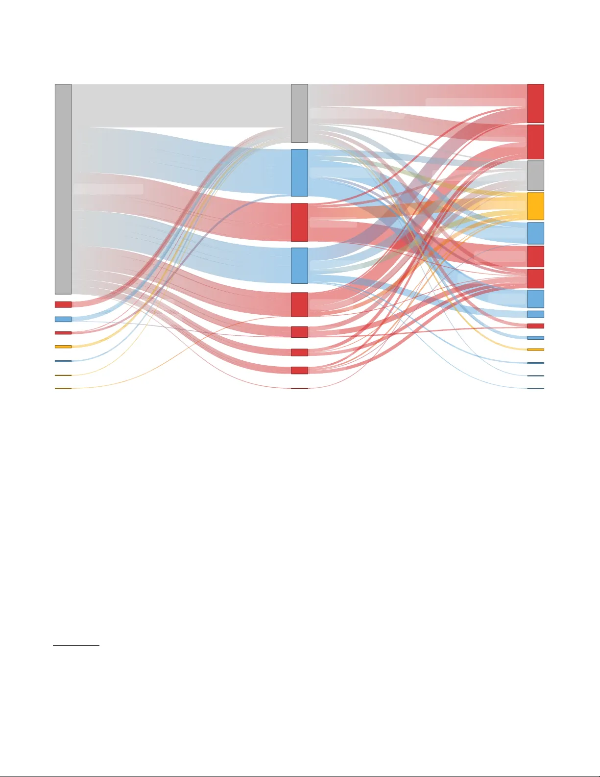
Beer Assumptions, Str onger Conclusions: The Case for Ordinal Regression in HCI Brandon Victor Syiem School of Computer Science The University of Sydney Sydney, NSW, A ustralia brandon.syiem@sydney.edu.au Eduardo V elloso School of Computer Science The University of Sydney Sydney, NSW, A ustralia eduardo.velloso@sydne y.edu.au Abstract Despite the widespread use of ordinal measures in HCI, such as Likert-items, there is little consensus among HCI researchers on the statistical methods used for analysing such data. Both parametric and non-parametric methods have b een extensively use d within the discipline, with limited reection on their assumptions and appropriateness for such analyses. In this paper , we examine recent HCI works that report statistical analyses of ordinal measures. W e highlight prevalent methods used, discuss their limitations and spotlight key assumptions and ov ersights that diminish the insights drawn from these methods. Finally , we champion and detail the use of cumulative link (mixed) models (CLM/CLMM) for analysing ordinal data. Further , we provide practical worked examples of applying CLM/CLMMs using R to published open-sourced datasets. This work contributes towards a better understanding of the sta- tistical methods used to analyse ordinal data in HCI and helps to consolidate practices for future work. CCS Concepts • Human-centered computing → HCI design and evaluation methods . Ke ywords Statistics, Ordinal Regression, Ordinal Data, Cumulative Link Mod- els, Cumulative Link Mixed Models A CM Reference Format: Brandon Victor Syiem and Eduardo V elloso. 2026. Better Assumptions, Stronger Conclusions: The Case for Ordinal Regression in HCI. In Proceed- ings of the 2026 CHI Conference on Human Factors in Computing Systems (CHI ’26), A pril 13–17, 2026, Barcelona, Spain. ACM, New Y ork, NY, USA, 21 pages. https://doi.org/10.1145/3772318.3790821 1 Introduction Ordinal measures, such as Likert-item surveys, score-based ques- tionnaires, and user preference rankings, ar e extensively used in HCI research. These measures enable researchers to gather quan- titative estimates of users’ subjective perceptions, psychological states, attitudes, preferences, judgements, and traits, allo wing direct comparative analysis between experimental conditions, other wise impossible thr ough qualitativ e data alone [ 60 ]. Despite the ubiquity This work is licensed under a Creativ e Commons Attribution 4.0 International License. CHI ’26, Barcelona, Spain © 2026 Copyright held by the owner/author(s). ACM ISBN 979-8-4007-2278-3/2026/04 https://doi.org/10.1145/3772318.3790821 and pertinence of such measures in HCI, there is a lack of consen- sus on the current statistical methods used to analyse such data. This has p otential long-term consequences that can hinder HCI researchers from aggregating, contrasting, and replicating ndings derived from ordinal data. Both parametric and non-parametric statistical methods are fre- quently encountered for analysing ordinal data in the HCI literature. Parametric methods, such as the one-way repeated ANO V A test, oer more statistical power when compared to their commonly used non-parametric counterparts, such as the Friedman test. How- ever , this increase in statistical pow er of parametric methods comes at the cost of str onger assumptions, typically on the distribution, ordering, and interval spacing of the data. Previous work has raised signicant concerns in analysing ordinal data with parametric meth- ods [ 12 , 37 ]. However , these concerns largely stem from the metric (order ed and evenly spaced intervals) handling of ordinal data in widely used methods, as opp osed to the method’s parametric nature. Analysing ordinal data with metric assumptions has been shown to increase T yp e I (false positives) and Type II (false negatives) errors, and even inverse the estimated means between groups [43]. Comparatively , non-parametric methods impose fewer assump- tions on data distribution and interval spacing. Importantly , most non-parametric methods do not treat ordinal data as metric, and are therefore seen as appr opriate for analysing such data [ 36 , 37 , 55 ]. Howev er , non-parametric methods are less sensitive, and could prevent researchers from dete cting existing eects [ 58 ]. More- over , ongoing debate regarding the metric/non-metric nature of data derived from ordinal measures, such as aggregated Likert scales [ 13 , 49 ], further complicate the selection of appropriate meth- ods. These challenges are particularly salient in HCI, wher e limited discourse [ 37 , 60 ] and the conation of concepts such as ‘metric’ and ‘parametric’ have produced inconsistencies in the statistical analysis of ordinal data. Such methodological disagreement in HCI research can lead to the propagation of erroneous insights, pr event methodologically distinct but related studies from being cross-examined, and hinder the process of deriving theory from empirical r esults. T o address these issues, we survey current HCI literature to better understand the dierent statistical methods used for analysing ordinal data. W e discuss the underlying mechanisms and assumptions used by frequently used methods in HCI, and deliberate on their appropri- ateness for handling ordinal data. W e then sp otlight and promote the use of cumulative link (mixed) mo dels, or CL(M)Ms, that ap- propriately treat ordinal data as categorical while leveraging the inherent ordering between the categories. W e explain the intuition and theory behind CL(M)Ms and detail its use and interpretation CHI ’26, April 13–17, 2026, Barcelona, Spain Syiem et al. through a practical demonstration on open-sourced HCI datasets using R. W e show that despite past criticisms of analysing ordinal data with metric assumptions, they continue to be frequently used in HCI research. This includes frequently use d parametric tests with known metric assumptions, as well as commonly use d non-parametric methods often regarded as appr opriate for ordinal data. Our nd- ings and discussion serve to better inform HCI researchers of the assumptions and pitfalls in current practices employed for statisti- cally analysing ordinal data. Finally , our description of CL(M)Ms and demonstration of its application using R on past open-sourced HCI data provide researchers with the information needed to ap- ply and interpret such methods — previously considered overly complex and inaccessible to HCI researchers [65]. 2 Background 2.1 Ordinal Measures, Likert-scales, and HCI Ordinal measures ar e categorical data that have inherent order- ing . T ake, for example , a sur vey item that asks participants to rate how satised they wer e with using a new image editing software on a scale of 1 to 5, with 1 b eing ‘V ery dissatised’ and 5 being ‘V ery satised’ . The participant’s response — a whole number scor e between 1 and 5 — is an ordinal measure that clearly indicates b etter user satisfaction as the rating goes up. How ever , ordinal data carry no metric information . This means that the distance between ordinal levels may not b e equal, and the labels are purely categorical with known ordering . A s such, the levels 1 to 5 in our example can be replaced by any other set of ordered categories, such as A to E or non-contiguous numerical labels (e.g., 1,2,7,16, and 41), without any loss of information. However , this also suggests that typical statistical methods that involve arithmetic operations to analyse or describe data, such as the data average, cannot be meaningfully interpreted when applied to ordinal data [45]. Despite such inhospitable properties to arithmetic op erations, contiguous numerical labels continue to b e the most frequently used labels for representing dierent levels of ordinal data. This numerical representation often leads ordinal data to be interpreted as an interval or ratio scale. How ever , the appropriateness of treat- ing ordinal data, and data derived from ordinal measur es, as met- ric has stirred considerable debate across multiple scientic disci- plines [13, 37, 43, 45, 60] that has spanned nearly a century [59]. This has not deterred the use of experimental methods that gen- erate ordinal data in scientic disciplines. HCI research, for example, widely makes use of ordinal measures in Likert-scales, sur veys and questionnaires, such as the NASA - TLX [ 33 ] or the system usability scale (SUS) [ 8 ]. Likert scales for instance, consist of multiple r elated survey items ( or Likert items), each with an ordinal response . Their widespread use in multiple disciplines, including HCI, psychology , economics, and medicine, among others [ 43 ], places them at the heart of the dispute surrounding ordinal data analysis. Despite these challenges, Likert scales are invaluable for collecting quantitative estimates of subjective phenomena otherwise unobtainable through qualitative data alone [60]. Likert scales present an additional dilemma to researchers, i.e., to analyse the scale as a single entity or to analyse individual Likert items. The prescribed method for analysing responses to Likert scales, as per Likert himself [ 44 ], was to aggregate (sum or average) responses to individual Likert items prior to analysis. This treats the data as metric, imposing assumptions so as to meaningfully apply arithmetic op erations for analysis. Numerous prior works, in various disciplines, have criticised this approach [ 36 , 43 , 45 ], stating that averaging ordinal data cannot produce interval scaled values. Others, however , have argued that aggregated ordinal data is perfectly suitable for metric interpretations, and can b e analysed using metric models given their robustness [13, 14, 55]. In contrast, r esearchers largely agr ee that individual Likert items, and Likert-type items [ 37 ] (single sur vey items with ordinal re- sponses that are independent of Likert scales), should not b e sta- tistically analysed using metric models [ 13 , 14 , 37 ]. Liddell and Kruschke [43] present strong arguments against treating averaged Likert scales and Likert-type items as metric, and demonstrate that the intuition behind the interval interpretation of averaged ordinal data is wrong. These disputes are ongoing, and we refrain from prescribing any single interpretation. Instead, w e highlight these disputes to demonstrate the extent and p ersistence of the disagree- ment surrounding ordinal data analysis, which continues to hinder analytical consistency and reproducibility within HCI. Additionally , HCI research also frequently employs methods other than Likert scales and Likert-type items that generate ordinal data [ 23 ]. A less obvious e xample of data interpretable as ordinal in HCI is that of a pre-/post-experiment test on topic understanding that results in a numerical score . While such a test score within a bounded numerical range (say range represented by 𝑅 ) intuitively seems to be metric, there is no guarantee that a score increase from 𝑥 to 𝑥 + 1 represents the same level of increase in understanding as a score increase from 𝑦 to 𝑦 + 1 (where { 𝑥 , 𝑦 } 𝜖 𝑅 ), as this would imply that all questions are equally dicult for all students. The extensive use of ordinal measures in HCI, combined with the in- conclusive disputes surrounding its treatment, warrants a deeper reection on the recent methods used to analyse ordinal data in HCI research. While past work has pr ovided insights into specic HCI subtopics [ 60 ] and suggestions for analysing ordinal data in HCI [ 37 , 65 ], there has been little reection on the frequency of use of ordinal measures, the methods used to analyse them, and methodological consensus within the eld. 2.2 The Parametric versus Non-parametric Debate While concerns about ordinal data analysis primarily stem from metric assumptions, the widespr ead use of parametric methods that impose these assumptions has le d prior work to discuss metric and parametric concepts interchangeably . Consequently , much of the debate surrounding ordinal data has regrettably shifted towards the appropriateness of parametric and non-parametric methods for analysis. For instance, commonly used parametric mo dels in HCI, such as ANO V A and Student’s t-test, place assumptions on the distribution of the data to enable meaningful statements to be made around arithmetic estimates, such as the mean and standard deviation. This makes such models appropriate when data can be interpreted as interval or ratio scale . In addition, these methods are not invariant to monotone transformations, i.e., transformations that change the absolute magnitude of the data while preserving Beer Assumptions, Stronger Conclusions: The Case for Ordinal Regression in HCI CHI ’26, April 13–17, 2026, Barcelona, Spain relative order . This makes them unsuitable for analysing ordinal data, as ordinal data contain no metric information, and any changes to the magnitude of scale labels should not aect analysis results. In contrast, most non-parametric models do not imp ose similar assumptions on data distribution, and are invariant to monotonic transformations. Instead, non-parametric models frequently en- countered in HCI, such as the Friedman test, transform the data into relative or dered ranks to further process for insights. For ex- ample, the ordered data sets of {5, 2, 3} (ordinal levels: 1 - 7) and {D, B, C} (order ed levels: A - G), will be ranked as {3, 1, 2}. This makes non-parametric models agnostic to changes in magnitude as well; distinct data groups containing {7, 1, 2} and {5, 1, 2} will similarly be ranked as {3, 1, 2} regardless of how much greater 7 is to 5 in the original data. Consequently , these methods are less sensitive to detecting eects when compared to their parametric counterparts, as the former ignores dierences in magnitude entirely . However , they are considered appropriate for ordinal data analysis as they impose less stringent assumptions [60]. In addition to sensitivity concerns, there is also a lack of accessi- ble non-parametric methods for analysing multi-factorial experi- mental designs for HCI researchers. Prior work has addressed this challenge by highlighting existing methods and pr oviding access to tools that enable non-parametric data analysis for multi-factorial designs [ 37 , 65 ]. For instance , Kaptein et al . [37] highlights existing non-parametric methods used in the medical eld for analysing Likert-type item data. Similarly , W obbrock et al . [65] introduces the aligned ranked transform (ART) method that enables practi- tioners to apply familiar and powerful multi-factorial ANO V A tests on transformed non-parametric data. Despite these eorts, there is still little consensus within the HCI discipline on how to best analyse ordinal data [23]. A largely neglecte d concern with using non-parametric methods for ordinal data analysis within HCI relates to test-specic assump- tions. Specically , while non-parametric methods can be use d to analyse ordinal data without imp osing the normality assumption (i.e., assuming that the residuals are normally distributed), they may still assume metric data . Non-parametric methods, such as the Wilcoxon Rank Sum T est 1 or the Friedman T est 2 , are examples of tests that do not assume normality of residuals or metric data. Therefore, these methods do not violate any of the properties of ordinal data, but do ignor e the dier ence in distances between ordi- nal le vels, which may r educe statistical power . In contrast, methods such as the Quade T est or the Wilcoxon Signed Rank T est for paired samples rst calculate the paired dierences prior to assigning ranks . This makes these tests unsuitable for strictly or dinal data as they perform arithmetic operations on data with no metric informa- tion [ 39 ]. Similarly , while it is suggeste d that the ART method can be used for ordinal data analysis [ 65 ], the process of ‘aligning’ or transforming the data in ART requires the calculation of av erages and residuals fr om the unaltered ordinal data, and, as such, imp oses metric assumptions on the data that may not be suitable for ordinal data. Imposing such assumptions is unlikely [ 59 ] to be problematic by themselves, provided the assumptions and possible drawbacks 1 ranks data points across both samples to be compared 2 ranks data points within each repeating block across all levels of a factor are made explicit to readers. However , more recent approaches have been developed that are specically designed to leverage the information held by ordinal data, without imposing incompatible assumptions on the data, such as with the use of cumulative link (mixed) mo dels, or CL(M)Ms. The availability of these methods, along with software and programming tools that make these meth- ods more accessible and practical to use, pr esents an opportunity to reconcile ordinal data analysis practices in HCI and move closer to more robust, theoretically informed, and reproducible ndings. 3 Review of Ordinal Analysis Practices in HCI T o understand current methodological practices for analysing ordi- nal data in HCI, we conducted a review of r ecent research articles published in the proceedings of the A CM CHI Conference on Hu- man Factors in Computing Systems (CHI). W e chose CHI based on its reputation as the agship confer ence for HCI research, and its broader representation of HCI topics (unlike more focused venues, such as ISMAR or Ubicomp). 3.1 Sampling As our aim was to understand recent statistical approaches for or- dinal data analysis in HCI, we restricted our search to the year 2024 and used a broad search string: [All Field: (“questionnaire ” OR “likert”)] . W e also limited our search to full papers. W e included papers that conducted user studies and reported statistical analyses of ordinal data. W e excluded papers that (1) did not include ordinal data, (2) focused on scale development and not on generating in- sights from analysing ordinal data, and (3) did not report analyses of included ordinal data beyond summary statistics. Our search resulted in 558 papers. W e randomly sample d 100 papers from the search results for full-text analysis. From the 100 sampled papers, we excluded 6 papers, resulting in a nal sample of 94 papers (details of the revie w steps are presented in Figure 1). For each paper , we recorded all ordinal measures collected and the associated construct. W e then recorded the statistical method used to analyse ordinal measures related to each construct. Note that a single paper could report multiple studies, and each study may collect multiple ordinal measures that may be analysed using multiple statistical methods. All extracted data can be found in our supplemental material. 3.2 Findings W e separate our ndings into three categories of statistical analysis methods; (1) statistical methods used to mathematically represent the data, and can be use d for parameter estimation and outcome pre- dictions in addition to hyp othesis testing — predictive modelling , (2) statistical methods used primarily for hypothesis testing involv- ing multiple factors and/or more than two groups — omnibus tests , and (3) statistical methods used primarily for hypothesis tests b e- tween two groups, or for performing multiple two group comparisons with corrections 3 (such as the Bonferroni correction) — pairwise comparisons/multiple pairwise comparisons . 3 Note that we do not extract data related to the specic corrections used during multiple pairwise comparisons CHI ’26, April 13–17, 2026, Barcelona, Spain Syiem et al. 55 8 p aper s impor t ed 100 full- t e xt p aper s assessed f or eligibili t y 6 p aper s e x c luded 1 Scale De v elopment 1 No Or dinal Dat a 4 No St atistical Anal y sis 94 p aper s inc luded 458 r andom sampling e x c lusions Figure 1: Overview of our review process detailing each step reported as per the PRISMA guidelines [ 47 ]. W e randomly sampled 100 papers from our initial search result of 558 papers. The full text of all 100 papers was screene d for eli- gibility . Six (6) papers were excluded, and the remaining 94 papers were included in our nal sample. 9 8 4 3 2 1 1 Linear Mixed-Effects Model Cumulative Link Mixed Model Linear Regression Model Generalised Estimating Equation Cumulative Link Model Generalised Linear Mixed Model PROCESS Model 7 Frequency Predictive Models Figure 2: Frequency of dierent predictive models reporte dly used for ordinal data analysis in our sample. Predictive mo delling. Only 28 instances of predictive mod- elling were reported for ordinal data analysis in our sample. Fig- ure 4 shows the frequency of the dierent reported mo dels used in our sample. Eight analyses used the Cumulative Link Mixed Model ( CLMM), 2 use d the Cumulative Link Model ( CLM), 3 uses of the Generalised Estimation Equation, 1 use of Generalised Linear Mixed Model ( with a logit link function — not cumulative logit which would class it as a CLMM), 9 instances of Linear Mixed- Eects Models, 4 Linear Regression Models, and 1 analysis using the PROCESS model 7 [34]. Omnibus tests. A total of 257 omnibus tests were reported to be used for ordinal data analysis in our sample. Figure 3 shows the frequency of the dierent reported tests. Parametric metho ds com- prised 71 reported uses of various Analysis of V ariance (ANOV A) tests, including 17 independent-sample ANO V A, 37 repeated-measure ANO V A (ANOV A-RM), 6 mixed-eects ANOV A ( ANO V A-ME), 1 Analysis of Covariance (ANCOV A), and 10 multivariate ANO V A (MANO V A). Reported non-parametric metho ds include 60 reported cases of the ART metho d to transform data prior to ANO V A analy- sis [ 65 ] (ART - ANO V A), 70 analyses using the Kruskal- W allis test, and 56 analyses using the Friedman test. 70 60 56 37 17 10 6 1 Kruskal-Wallis test ART-ANOVA Friedman test ANOVA-RM ANOVA MANOVA ANOVA-ME ANCOVA Frequency Omnibus Methods Figure 3: Frequency of dierent omnibus tests used for ordi- nal data analysis in our sample. 61 54 39 34 33 30 28 11 7 5 3 2 1 1 Wilcoxon Signed Rank test Paired t-test Unspecified Wilcoxon Rank Sum test ART-Contrast Independent t-test Dunn test Conover test Tukey HSD Chi-Squared test EMMs Comparison Nemenyi test Games-Howell test Kolmogorov-Smirnov test Frequency Pairwise Comparison Methods Figure 4: Frequency of dierent pairwise comparisons re- portedly used for ordinal data analysis in our sample. Pairwise comparisons. 309 pair wise comparisons were report- edly conducted for ordinal data analysis in our sample. Figure 4 shows the frequency of the dierent reported tests. Parametric tests were dominated by paired (54) and independent-sample t- tests (30), with a minority employing the T ukey Honest Signicant Dierence (T ukey HSD) test (7). Non-parametric tests primarily consisted of the Wilcoxon Signed Rank test (61) for paired samples, and the Wilcoxon Rank Sum test (34) for independent samples. Other non-parametric tests observed include the Chi-squared test (5), the Dunn test (28), the Conover test (11), Games-Howell test (1), the Kolmogorov-Smirno v test (1), the Nemenyi test (2), and the ART -Contrast tests (33) following the ART - ANO V A tests. Addition- ally , we found three (3) instances of pairwise comparisons based on estimated marginal means (EMMs Comparison). Note that ‘EMMs Comparison’ is not a single statistical test, but refers to post-hoc pairwise comparisons of estimated marginal means derived from a tted model [ 42 ]—observed following 1 GLMM and 2 CLM model ts in our sample 4 . Finally , we found multiple post-hoc tests in our sample that did not specify the exact test used and simply referred to pairwise comparisons as ‘post-hoc analysis/test’ . This accounted for 39 instances in our sample, labelled as ‘unspecie d’ . 3.3 Discussion A n undecided discipline: Our review demonstrates the use of numerous statistical approaches for analysing ordinal data in HCI 4 W e classify ‘EMMs Comparison’ as parametric because estimated marginal means depend on model parameters. However , it can also be applie d in non-parametric contexts, such as post-hoc comparisons following an ART - ANO V A model t Beer Assumptions, Stronger Conclusions: The Case for Ordinal Regression in HCI CHI ’26, April 13–17, 2026, Barcelona, Spain No model reported Linear Mixed-Effects Model PROCESS Model 7 Generalised Linear Mixed Model Linear Regression Model Cumulative Link Mixed Model Generalised Estimating Equation Cumulative Link Model ANCOV A MANOV A ANOV A-ME ANOV A ANOV A-RM Friedman test ART -ANOV A Kruskal-W allis test No omnibus test reported Wilcoxon Signed Rank test Paired t-test Unspecified No pairwise test reported Wilcoxon Rank Sum test ART -Contrast Independent t-test Dunn test (Ranked) Games-Howell test Kolmogorov-Smirnov test Nemenyi test EMMs Comparison Chi-Squared test Conover test T ukey HSD Figure 5: Sankey diagram showing the progression of statistical procedures applied to constructs measured with ordinal data. Methods are displayed in sequence from predictive models (left), to omnibus tests (centre), to pair wise tests (right). Bars lab elled ‘No’ indicate constructs for which no method was reported in that categor y . Re d nodes indicate statistical methods that impose incompatible assumptions with ordinal data, blue nodes represent ordinal data compatible metho ds, yellow nodes represent methods whose appropriateness for analysing ordinal data is dependent on specic factors (such as the link’ function use d), and grey no des represent absent methods in that spe cic category . As seen in the Figure, our sample reported limited use of predictive models (No model reported), and most models and omnibus approaches were not frequently used together (most models have links to ‘No omnibus test reported’). The Figure also clearly highlights a lack of consensus within the eld; with no clear direction of which method, or sequence of methods, should be used to analyse ordinal data. research. Both parametric and non-parametric methods continue to be frequently used, with non-parametric appr oaches outnumbering parametric approaches (362 5 against 165 6 respectively , excluding unspecied pairwise comparisons and predictive models; as mo dels are dependent on the link function used). The increased use of non- parametric methods suggests a trend towards adopting approaches that impose fewer assumptions on ordinal data for analysis. How- ever , we obser ved 154 cases of the use of the non-parametric ap- proaches that assume data to be metric. These include 60 cases of the ART -ANOV A test, 33 cases of the post-ho c ART -Contrasts test, and 61 cases of the Wilcoxon signed rank test. This suggests that a 5 60 ART -ANOV A + 70 Kruskal-W allis tests + 56 Frie dman tests + 33 ART-Contrast + 5 Chi-squared test + 28 Dunn test + 11 Conover test + 1 Games-Howell test + 1 Kolmogoro v-Smirnov test + 2 Nemenyi test + 34 Wilcoxon Rank Sum test + 61 Wilcoxon Signed Rank test 6 17 ANO V A + 37 ANOV A.RM + 6 ANO V A.ME + 1 ANCOV A + 10 MANO V A + 3 EMMEANS + 30 independent t-test + 54 paired t-test + 7 Tuke y HSD total of 319 out of 527 tests in our sample (excluding models and unspecied pair wise comparisons) impose metric assumptions on ordinal data. It is unclear if this is the result of widespread mis- interpretation of the term ‘non-parametric’ to also e xclude metric assumptions on the data or an informed decision to treat ordinal data as metric . In either case, this presents a challenge for futur e scholars in consistently interpreting, contrasting and building upon ndings related to ordinal data that r ely on dierent data assumptions. T o better inform practitioners, we present the relevant assumptions for ordinal data analysis of the dier ent hypothesis tests (omnibus and pairwise comparisons) found in our sample in Table 1. The table excludes predictive models as their assumptions are dependent on additional factors, such as the ‘link’ function used. Inconsistent successive assumptions: Our ndings further reveal that current HCI practices for analysing ordinal data may CHI ’26, April 13–17, 2026, Barcelona, Spain Syiem et al. Omnibus or Pairwise Method Category Experimental Design Assumption Metric Data Normality of Residuals Equal V ariance Wilcoxon Signed Rank test [39, 63] Pairwise Within-Subject Design ✓ ✗ ✗ Wilcoxon Rank Sum test [63] Pairwise Between-Subject Design ✗ ✗ ✗ ART -Contrasts [25] Pairwise Mixed Design ✓ ✗ ✗ Dunn test [22, 24] Pairwise Between-Subject Design ✗ ✗ ✗ Conover test [19, 20, 54] Pairwise Between/Within-Subject Design ✗ ✗ ✗ Chi-squared test [52] Pairwise Between-Subject Design ✗ ✗ ✗ Nemenyi test [48] Pairwise Within-Subject Design ✗ ✗ ✗ (Ranked) Games-Howell test [30, 57] Pairwise Between-Subject Design ✗ ✗ ✗ Kolmogoro v-Smirnov test [4] Pairwise Between-Subject Design ✗ ✗ ✗ Kruskal- W allis test [40] Omnibus Between-Subject Design ✗ ✗ ✗ ART -ANOV A [65] Omnibus Mixed Design ✓ ✗ ✗ Friedman test [28] Omnibus Within-Subject Design ✗ ✗ ✗ Sampled Parametric Methods — — ✓ ✓ ✓ T able 1: Table detailing common assumptions relevant to ordinal data analysis for omnibus and pairwise methods found in our sample. The table lists the categor y of the statistical method, the experimental design that generates data suitable for the method to analyse, and the assumptions that the metho d imposes. The table primarily details sampled non-parametric methods, as all parametric omnibus & pairwise tests in our sample (not all existing parametric methods) assume metric data, normality of residues, and equal variance — and are hence collectively repr esented by the last row . Notably , this table highlights frequently used non-parametric methods in HCI that exhibit incompatible assumptions on ordinal data. Specically , the Wilcoxon Signed Rank test, the ART -Contrasts and the ART -ANOV A impose metric assumptions on the data (via the use of arithmetic operations on unranked data). Note that this table excludes approaches that we categorize as predictive models (e.g., CLMs or GLMs), as their assumptions depend on additional factors such as the ‘link’ function. impose inconsistent data assumptions across the sequence of sta- tistical procedures applied to ordinal data within the same study . T ake, for example , the pairwise tests following a Friedman test (ap- propriate for repeated-measure non-parametric data) in our sample as depicted in Figure 5. This includes the Wilcoxon Signed Rank test, the Conover test, the Games-Howell test and the Nemenyi test, among additional unspecie d tests. These tests are all ap- propriate for analysing non-parametric data generated through a within-subject experimental design. Howe ver , they dier in their treatment of the data, and may unintentionally impose assumptions incompatible with ordinal data that was initially avoided in the preceding omnibus test. For instance, the most frequently use d test following the Friedman omnibus test in our sample was the Wilcoxon Signed Rank test, which assumes metric data , unlike its preceding omnibus test (see T able 1). This inconsistent treatment of ordinal data within individual se quences of analyses further complicates the interpretation of ordinal data analysis, which is already challenged by the parametric and non-parametric debate. Such inconsistencies warrant a change in the current statistical methods used for ordinal data analysis within HCI, prompting the need for methods that address the concerns stemming from ov er- or under-estimating the information present in ordinal data [11]. Ordinal rst modelling: Spe cically designed predictive mod- eling te chniques, known as ordinal regression models (e.g., CL(M)Ms), provide greater statistical pow er than non-parametric approaches while avoiding the incompatible assumptions of commonly used parametric methods in HCI, such as ANO V As. They achieve this by leveraging the ordinal structure of the data without assuming equally spaced intervals between categories. However , such mo dels see limited application in HCI (see Figure 2). A possible explana- tion for such limited use, is the focus on the use of ordinal data for hypothesis testing in recent HCI work, as corroborated by the disparity between the frequency of hypothesis tests (omnibus and pairwise tests) and predictive modelling methods in our sample (Figures 3, 4, and 2). This could further be explained by previous challenges in understanding, interpreting and applying predictive modelling metho ds in HCI research [ 65 ]. However , we argue that re- cent developments in statistical analysis software have made these methods increasingly more accessible and easy to apply . T o b etter inform HCI practitioners in understanding and using the methods, the following sections describ e the proposed CL(M)M modelling technique, and presents worked examples using CL(M)Ms to anal- yse ordinal data in published open source HCI data. W e additionally provide an interactive tool in our supplementar y material to illus- trate a simple CLM model. 4 Cumulative Link (Mixe d) Models Cumulative Link (Mixed) Models, or CL(M)Ms, are a class of Gen- eralised Linear (Mixed) Models that ar e designed for ordinal regres- sion. Throughout this paper , we will often use the term ‘CL(M)M’ to r efer to both cumulative link mo dels (CLMs) and cumulative link mixed models (CLMMs). Specically , CLMs are appropriate when only xed eects are of interest and observations can be assumed to be independent. In contrast, CLMMs extend CLMs by incorpo- rating random ee cts, allowing them to account for grouped or hierarchical data in which the independence assumption is violated (e.g., repeated-measures experimental designs). These models ap- propriately treat ordinal data as categorical , while exploiting the Beer Assumptions, Stronger Conclusions: The Case for Ordinal Regression in HCI CHI ’26, April 13–17, 2026, Barcelona, Spain ordered nature of the data [ 17 ]. Given such advantages, these meth- ods are increasingly encourage d and used for modelling ordinal data in diverse elds of research, including psychology [ 11 , 29 , 43 ], econometrics [ 38 ], machine learning [ 64 ], and health [ 15 ]. Despite the advantages of CL(M)Ms, they have been largely overlooked in HCI, due to challenges in understanding, interpr eting and applying these methods [ 65 ]. As with all statistical methods, CL(M)Ms come with their own set of assumptions that are important to understand and consider prior to their use. With the incr easing availability of software packages capable of performing ordinal regression using CL(M)Ms [ 2 , 17 ] in popular statistical tools, such as Stata, R, and Python, this section provides an intuitive description of the the- ory and assumptions of CL(M)Ms in the context of HCI research. Readers already familiar with CL(M)M theor y and assumptions, or those interested primarily in practical applications of CL(M)Ms for HCI data, may skip to Section 5. 4.1 Intuition Say that we are inter ested in the eect of adding a new feature to our system (e.g. faster scr een frame rate) on an element of user ex- perience (e.g. spatial pr esence in virtual reality). In an ideal scenario, we would have a tool that could directly measure a user’s sense of spatial presence, giving us a continuous and normally distributed measure that we could analyse using a familiar method, such as an ANO V A. Figure 6 illustrates this ideal scenario. Figure 6: Ideally , we could directly measure a user’s sense of spatial presence from their thoughts (LEFT). If the measure is continuous and normally distributed (RIGH T), it would enable us to use familiar metric models of statistical analysis and comparisons. Howev er , constructs such as spatial presence are not directly observable, and conse quently , require us to use proxy measur es. Of- ten, Likert-item style d questionnaires are used, wher e users provide a rating of spatial presence on an ordinal scale. Unlike metric data, ordinal data do not exhibit equal distances between ratings, i.e., the ordinal values of 3 − 2 and 5 − 4 may not be equal, e ven if they se em to arithmetically equate to 1 due to the use of contiguous numerical labels. As such, ordinal values cannot b e meaningfully analysed using methods that rely on arithmetic op erations. In the context of our example, this means that we cannot estimate how much more spatially present users were (on average) when using our system with, and without, the new feature by subtracting the aver- age ordinal responses for the dierent system conditions. Figure 7 illustrates these dierences between the continuous representation in our ideal case (left), and the ordinal measure collected in a real- world context (right). In the ideal scenario, users’ spatial presence scores with and without the added feature form two normal dis- tributions, and the average ee ct of the new feature is reecte d by the shift from the original distribution. In reality , howev er , we can only collect user spatial presence measures via ordinal ratings on a predened scale (say from 1 to 5), resulting in distributions of ordinal data (right) that is far fr om normal, and whose eect is much harder to estimate. A v e r a g e Ef f e c t Figure 7: Figure depicting an ideal scenario and our reality when deriving insights from ordinal data related to our sys- tem. In an ideal scenario (LEFT), we would not need ordinal measures, and we would have direct and continuous mea- sures of users’ spatial presence when using the two versions of our system. This would result in two distinct normal dis- tributions of users’ spatial presence when using our system with and without the new feature. In reality (RIGHT), spatial presence cannot be measured directly and instead a discrete score (e.g., b etween 1 and 5) is provided by the user to in- dicate their level of spatial presence under the two system variations. CLMMs attempt to address this challenge by taking a principle d approach to analysing ordinal data. These models assume that there exists a continuous unobservable measure (or latent variable) in the user’s mind that underlies an obser vable ordinal measure. Since this measure is unobservable, the unit of measurement can b e arbitrary . Conventionally , CL(M)Ms assume that this latent variable is distributed with a standard normal (0,1) distribution (though models can be extended into any arbitrar y latent distribution). If indeed the obser ved scores reect these assume d underlying latent values, then they should b e statistically related. How ever , CL(M)Ms do not assume this relationship to be linear , only monotonic (i.e. as the latent value increases, so does the likelihood of a higher user rating). Imagine a user who initially experiences no spatial presence (i.e. their latent score should be the minimum imaginable). This user would most likely give the lowest possible rating (1 - V er y low). A s we intervene to increase the latent score from its absolute minimum, we would still see scores of 1 until we reach a certain level, at which point, we would start seeing scores of 2. A s we keep increasing the latent score and reaching these thresholds/cutpoints, our ratings should increase accordingly . Because the latent normal and the observed scores distributions are connected under these assumptions, we can also assume that the proportion of users with a latent value between any 2 cutpoints should be equal to the proportion of users that gave the correspond- ing rating. As such, we can compare the cumulative distribution of the scores to the cumulative distribution of the latent normal. In other words, if 10% of our scores were 1, and we kno w that in CHI ’26, April 13–17, 2026, Barcelona, Spain Syiem et al. Figure 8: Our ordinal rating increases when the latent value increases beyond a cutpoint. By looking at which cutpoints the latent value falls b etween, we can predict which score the user would give . a standard normal distribution 10% of values ar e lower than -1.28, then we can say that -1.28 is the cutpoint in the latent scale at which someone’s rating would go from 1 to 2. If in the same dataset we found that 15% of scores were 2, we would have to look for the 15 + 10 = 25% quantile of the normal distribution to nd the next cutpoint—in this case, -0.67. W e can proceed the same way for the other cutpoints. Figure 8 visualizes the selection of ordinal scores based on the cutpoints that divide the latent measure scale. This method gives us a way to r etrieve the latent cutpoints fr om observed scores. Howev er , ultimately , we are interested in the causal eect of our inter vention. For this example, we will assume that the intervention only shifts the mean of our latent distribution (not the variance). Under the same cutpoints, shifting the mean of the latent measur e causes the area under the normal curve between the cutpoints to change—and these areas are precisely the pr oportion of each of the possible ratings. Figure 9 shows this process. W e infer the cutpoints from the baseline ratings, shift the mean of the normal distribution to the left (which implies an average decrease in the latent value) and see how it aects the distribution of scores. W e oer a Shiny app in the supplementary material where you can set the cutpoints and observe how dierent eect sizes aect the distribution of scores. So far , we describ ed the intuition of the method generatively , that is, from the user’s mind to the scores. In essence, CL(M)Ms do the inverse of this process: they take ordinal ratings and dir ectly estimate the eects on the latent scale. Our example uses the cu- mulative proportion analogies to build an intuition. In practice, howev er , the cutp oints are not simply derived from the cumula- tive proportions of observed scores, but jointly estimated from the data along with the model coecients. Next, we provide a more formal mathematical description of how it works and a practical implementation in R. 4.2 Theory and Mathematics As a predictive model, CL(M)Ms model the relationship between a dependent variable and predictor/independent variable(s). Let us extend the example used in section 4.1 to illustrate this. Say we ask − 3 − 2 − 1 0 1 2 3 − 3 − 2 − 1 0 1 2 3 Figure 9: From a given distribution of baseline scores, we can infer the latent cutpoints and predict how shifting the mean of the distribution would ae ct the distribution of scores accordingly . participants to use dierent v ersions of our system (a categorical in- dependent variable repr esented as 𝑋 ) and rate their sense of spatial presence b etween 1 and 5, with 1 being ‘V ery low’ and 5 being ‘V ery high’ (an or dinal dependent variable represented as 𝑌 ). W e can r ep- resent this relationship as a causal graph, 𝑋 → 𝑌 , where the arrow pointing from 𝑋 (system version) to 𝑌 (spatial presence r esponse) indicates that 𝑋 has a causal eect on 𝑌 . In this scenario, the goal of predictive modelling would b e to describe how changing the system version 𝑋 inuences user responses about their sense of spatial presence 𝑌 , i.e., how 𝑋 predicts 𝑌 . Howev er , the ordinal response, 𝑌 , is an imperfect measure that the user generates about their sense of spatial presence in using a system version, based on some in- ternal psychological measure and the available ordinal responses (elaborated in the example presented in gure 7). For example, a user’s true spatial presence experience may lie somewhere between Beer Assumptions, Stronger Conclusions: The Case for Ordinal Regression in HCI CHI ’26, April 13–17, 2026, Barcelona, Spain Figure 10: Figure illustrating the relationship b etween the internal continuous latent variable e 𝑌 with the observable or- dinal response 𝑌 in our spatial presence example. Here, a user determines the system to elicit ‘V ery low’ spatial presence when their internal measure falls below the rst cutpoint ( 𝜏 1 ), ‘Low’ spatial presence , when their internal measure is between the rst ( 𝜏 1 ) and second ( 𝜏 2 ) cutpoints, and so on. ‘High’ (scale value 4) and ‘V ery High’ (scale value 5), but the limited response options force a decision that imperfe ctly captures the user’s true experience. Additionally , there is no guarantee that the internal psychological distance between two or dinal responses is evenly spaced. For instance, users may nd it easy to change their response from 3 (‘Moderate’) to 4 (‘High’) — small psychological distance — but may reserve the highest response of 5 (‘V er y high’) to systems that they perceive as e xceptional at evoking a sense of spatial presence — large psychological distance b etween 4 and 5 when compared to 3 and 4. This prev ents meaningful analysis that relies on these distances to b e consistent, such as statistical analysis methods that calculate averages or dierences, and is a key cause of errors in analysing ordinal data using metric models [11, 43]. CL(M)Ms account for the internal psychological measure by as- suming the presence of an underlying continuous latent (unobserv- able) variable (represented as e 𝑌 ). This results in an updated causal graph, 𝑋 → e 𝑌 → 𝑌 , which explicitly represents how the system version ( 𝑋 ) aects an internal psychological measure of the user’s sense of spatial presence ( e 𝑌 ), which is then categorized into an ordinal response ( 𝑌 ). Given this new causal structure, the r elation- ship between the observable response, 𝑌 , and the latent var iable, e 𝑌 , can then be dene d using a set of ordered thresholds/cutpoints, which determines the value that 𝑌 categorizes to, when e 𝑌 falls within certain cutpoints . In our example, the 5 dierent responses (‘V ery low’ to ‘V ery high’) will need 4 cutpoints (repre- sented as 𝜏 = { 𝜏 1 , 𝜏 2 , 𝜏 3 , 𝜏 4 } ) to categorize all 5 available ordinal response, i.e, 𝑌 = 1 (‘V ery low’) when e 𝑌 ≤ 𝜏 1 , 𝑌 = 2 (‘Low’) when 𝜏 1 < e 𝑌 ≤ 𝜏 2 , and so on, with the highest value, 𝑌 = 5 (‘V ery high’) manifesting when 𝜏 4 < e 𝑌 . This process is illustrated in Figure 10 (and with a familiar Likert item example in gur e 8). In general, if we have 𝐾 dierent ordinal r esponses, we will need 𝐾 − 1 cutpoints. Formally: 𝑌 = 𝑘 if 𝜏 𝑘 − 1 < e 𝑌 ≤ 𝜏 𝑘 (1) This conceptualization of the latent continuous variable, e 𝑌 , en- ables CL(M)Ms to mathematically express 𝑌 in terms of e 𝑌 and 𝜏 . CL(M)Ms can then model the continuous latent variable e 𝑌 in re- lation to 𝑋 using linear regression. Collectively , these two steps enable CL(M)Ms to describe the relationships represented in the causal graph: 𝑋 → e 𝑌 → 𝑌 . T o express 𝑌 in terms of e 𝑌 and 𝜏 , CL(M)Ms must rst ensure that the observable ordinal data ( 𝑌 ) is appropriately tr eated as cate- gorical , avoiding over-representation of information (as with metric modelling approaches) [ 11 ]. However , treating ordinal data as cate- gorical exposes only frequencies/probabilities as quantitative infor- mation, which ar e devoid of any ordering (under-representing avail- able information as with most non-parametric approaches [ 11 ]). For example, the pr obability set {0.2, 0.1, 0.7} corresponding to an ordered dataset with levels { A, B, C} provides no information about the ordering of the data. T o remedy this, CL(M)Ms make use of cumulative probabilities in place of individual probabilities. This ensures that higher order ed categories are always associated with higher cumulative probabilities and vice-v ersa. Extending our ex- ample, the ordered dataset with levels {A, B, C} and probabilities {0.2, 0.1, 0.7}, will exhibit cumulative probabilities of {0.2, 0.3, 1.0} 7 , pre- serving order . This also enables us to extract individual probabilities from cumulative probabilities using: 𝑃 ( 𝑌 = 𝑘 ) = 𝑃 ( 𝑌 ≤ 𝑘 ) − 𝑃 ( 𝑌 ≤ 𝑘 − 1 ) (2) Now , from (1) , we can infer that 𝑌 ≤ 𝑘 when e 𝑌 ≤ 𝜏 𝑘 . There- fore, we can relate the cumulative probability 𝑃 ( 𝑌 ≤ 𝑘 ) with the cumulative probability 𝑃 ( e 𝑌 ≤ 𝜏 𝑘 ) which can be calculated using a cumulative distribution function over e 𝑌 , represented as 𝐹 ( 𝜏 𝑘 ) . Here, the function 𝐹 depends on the assumed distribution of e 𝑌 . T wo commonly used distributions include the standard logistic dis- tribution and the standard normal distributions, which hav e been referred to by the names order ed logit models and ordered probit models respectively [ 32 ]. The choice of assumed distribution inu- ences the interpretation of the results but often results in similar parameter estimates and model ts [ 46 ]. For the purposes of this paper , we assume that e 𝑌 follows a standard normal distribution. Details related to the dier ent distributions and their corresponding cumulative distribution functions can be found in prior w ork [ 1 , 11 ]. Given the function 𝐹 , w e can now expr ess the relationship between 𝑌 and e 𝑌 as: 𝑃 ( 𝑌 ≤ 𝑘 ) = 𝑃 ( e 𝑌 ≤ 𝜏 𝑘 ) = 𝐹 ( 𝜏 𝑘 ) (3) From equation (2) and (3) , we can determine individual proba- bilities of ordinal responses based on the cumulativ e distribution function ( 𝐹 ) and the cutpoints ( 𝜏 ): 𝑃 ( 𝑌 = 𝑘 ) = 𝐹 ( 𝜏 𝑘 ) − 𝐹 ( 𝜏 𝑘 − 1 ) (4) Howev er , e quation (4) does not explain the inuence of system version ( 𝑋 ) on spatial presence response ( 𝑌 ). T o account for this, CL(M)Ms use linear regression to model the continuous latent vari- able e 𝑌 with respect to 𝑋 8 : e 𝑌 = 𝑋 𝑇 𝛽 + 𝜀 (5) Where the coecient 𝛽 in the linear predictor ( 𝑋 𝑇 𝛽 ) describes the change in e 𝑌 with respect to unit change in 𝑋 , and 𝜀 is the 7 Each value in this array is obtained by adding up all prece ding values in the original array . 8 While w e illustrate using a single independent variable, CL(M)Ms can handle multiple independent variables, where X would represent a matrix of column vectors. CHI ’26, April 13–17, 2026, Barcelona, Spain Syiem et al. Figure 11: Figure showing example distributions of e 𝑌 for 𝑋 = 𝑉 𝑒 𝑟 𝑠 𝑖 𝑜 𝑛 1 ( e 𝑌 = 𝑋 𝑇 1 𝛽 1 + 𝜀 ) and for 𝑋 = 𝑉 𝑒 𝑟 𝑠 𝑖 𝑜 𝑛 2 ( e 𝑌 = 𝑋 𝑇 2 𝛽 2 + 𝜀 ). The gure presents an example where users are more in- clined to respond with a higher spatial presence rating to 𝑉 𝑒 𝑟 𝑠 𝑖𝑜 𝑛 2 compared to 𝑉 𝑒 𝑟 𝑠 𝑖𝑜 𝑛 1 . This is depicted by the larger proportion of the curve (area under the curve) for 𝑉 𝑒 𝑟 𝑠 𝑖𝑜 𝑛 2 that falls b etween cutpoints ( 𝜏 ) that dene higher ordinal re- sponses, when compared to the curve for 𝑉 𝑒 𝑟 𝑠 𝑖𝑜 𝑛 1 . For exam- ple, area under the curve for 𝜏 4 < e 𝑌 , dening the probability of a ‘V ery high’ user response, is larger for 𝑉 𝑒 𝑟 𝑠 𝑖𝑜 𝑛 2 than for 𝑉 𝑒 𝑟 𝑠 𝑖𝑜 𝑛 1 random error describing the assumed distribution of e 𝑌 (standard normal in this example). T o elaborate, let us assume that our spatial presence study example tests two system versions ( 𝑋 1 = V ersion 1 and 𝑋 2 = V ersion 2 ), with the rst version having slower screen frame rate than the second version. This can be represented in our linear model of e 𝑌 as two binary (0 or 1) variables 𝑋 1 and 𝑋 2 , indicating the presence or absence of that system version. Therefore, for this example, we can specify equation (5) as: e 𝑌 = 𝑋 𝑇 1 𝛽 1 + 𝑋 𝑇 2 𝛽 2 + 𝜀 (6) Since a user can only experience one version at a time in our experiment that compares the tw o versions, either 𝑋 𝑇 1 𝛽 1 or 𝑋 𝑇 2 𝛽 2 will be equal to zero. Ther efore, our linear pr edictor for e 𝑌 can be described as: e 𝑌 = ( 𝑋 𝑇 1 𝛽 1 + 𝜀 , if 𝑋 = 𝑉 𝑒 𝑟 𝑠 𝑖 𝑜 𝑛 1 𝑋 𝑇 2 𝛽 2 + 𝜀 , if 𝑋 = 𝑉 𝑒 𝑟 𝑠 𝑖 𝑜 𝑛 2 If V ersion 1 and 2 yield dierent eects on the latent spatial presence variable e 𝑌 (i.e., 𝛽 1 ≠ 𝛽 2 ), then e 𝑌 will exhibit dierent distribution positions for dierent system versions. As such, we can estimate the causal eect of switching from V ersion 1 to V ersion 2 by subtracting their respective means. Figure 11 illustrates the distribution of the latent spatial presence variable e 𝑌 when users respond with a higher spatial presence rating for V ersion 2. Collectively , we now have equation (3) that describes the rela- tionship between the user’s response ( 𝑌 ) and their internal spatial presence measure ( e 𝑌 ), and equation (5) that models a linear rela- tionship between the internal measure ( e 𝑌 ) and the system version ( 𝑋 ). Therefore, we can model the probability of a user response ( 𝑌 ) being less than a sp ecied value 𝑘 given the linear predictor ( 𝑋 𝑇 𝛽 ) of e 𝑌 as: 𝑃 ( 𝑌 ≤ 𝑘 | 𝑋 𝑇 𝛽 ) = 𝑃 ( e 𝑌 ≤ 𝜏 𝑘 | 𝑋 𝑇 𝛽 ) = 𝑃 ( 𝑋 𝑇 𝛽 + 𝜀 ≤ 𝜏 𝑘 ) = 𝑃 ( 𝜀 ≤ 𝜏 𝑘 − 𝑋 𝑇 𝛽 ) = 𝐹 ( 𝜏 𝑘 − 𝑋 𝑇 𝛽 ) (7) In practice, equation (7) is expressed in terms of the inverse cumulative distribution function ( 𝐹 − 1 ) which is the ‘link’ function in generalise d linear models to connect the linear predictor with the response value (see Agresti and Kateri [1] for a detailed description of these functions). Given (7) , we can update equation (4) to consider the linear predictor ( 𝑋 𝑇 𝐵 ) of e 𝑌 to express the probability of 𝑌 at individual responses as: 𝑃 ( 𝑌 = 𝑘 | 𝑋 𝑇 𝛽 ) = 𝐹 ( 𝜏 𝑘 − 𝑋 𝑇 𝛽 ) − 𝐹 ( 𝜏 𝑘 − 1 − 𝑋 𝑇 𝛽 ) (8) This gives us the nal equation that describes the relationship between the system version ( 𝑋 ) and the obser vable spatial pr esence user rating ( 𝑌 ). 4.3 Assumptions Like any statistical analysis method, CL(M)Ms impose a set of as- sumptions that should be carefully considered prior to their appli- cation. While we briey mention these assumptions in se ctions 4.1 & 4.2, we elab orate on them here for further consideration. Addition- ally , tools to test for , and relax, some of the discussed assumptions are available with most software implementations for ordinal data analysis (see examples in R [ 17 ] and Stan [ 11 ]). If readers ar e not inclined towards making certain assumptions, and if these assump- tions cannot be relaxed, they can refer to our table 1 for support in selecting alternative statistical tests to analyse their ordinal data. Latent V ariable Assumption. A fundamental assumption of CL(M)Ms relevant to HCI is that there exists an internal psycho- logical measure ( or latent variable) with an assumed distribution (standard normal in our ‘probit link’ examples) that dictates, based on cutpoints, the ordinal response of a user to a sp ecic sur vey question or Likert-item. The assumption of underlying latent vari- ables is prominent and relevant in many elds, and particularly in psychology and the social sciences [ 5 ] where studies often focus on phenomena with directly unobservable causes. However , it is still worth considering whether such an assumption aligns with the researchers’/analysts’ beliefs prior to the use of CL(M)Ms (or similar) for their analysis. Latent Equal- V ariance Assumption. Heretofore, w e have de- scribed CL(M)Ms using simplied examples that only illustrate changes in the location (distributional position) of the underlying latent variables e 𝑌 (see gure 7, 9, & 11). While standard CL(M)Ms assume constant variance of e 𝑌 , they can be extended to account for unequal variances by modelling the scale (standard deviation, 𝜎 ) of e 𝑌 within the model [ 17 ]. Practically , 𝜎 can be incorporated through an additional regression factor in the model, often expressed as its inverse [ 11 ] ( 𝛼 = 1 / 𝜎 ). Accor dingly , equation (7) takes the form: 𝑃 ( 𝑌 ≤ 𝑘 | 𝑋 𝑇 𝛽 , 𝛼 ) = 𝐹 ( 𝛼 × ( 𝜏 𝑘 − 𝑋 𝑇 𝛽 ) ) . Where, 𝛼 = 𝑒 𝑥 𝑝 ( 𝑋 𝑇 𝛽 𝛼 ) to ensure 𝛼 > 0 , and 𝑋 𝑇 𝛽 𝛼 is the linear predictor for 𝛼 . Modelling the scale as an additional regr ession factor enables the variance of e 𝑌 to also be dependent on the variables 𝑋 . More in-depth details can be found in Bürkner and Vuorr e [11]. Proportional Odds Assumption. Another important assump- tion of CL(M)Ms is dubbed the proportional odds assumption . This Beer Assumptions, Stronger Conclusions: The Case for Ordinal Regression in HCI CHI ’26, April 13–17, 2026, Barcelona, Spain assumption refers to the unchanging co ecient estimates ( 𝛽 ) across all cutpoint estimates ( 𝜏 = { 𝜏 1 , 𝜏 2 , . . ., 𝜏 𝑘 − 1 } ), i.e., the coecients ( 𝛽 ) remain the same ∀ 𝑘 = { 1 , 2 , . . ., 𝐾 − 1 } in 𝑃 ( 𝑌 = 𝑘 | 𝑋 𝑇 𝛽 ) in equation (8) . Equivalently , this assumes that the cutpoints do not individually vary based on the independent variables ( 𝑋 ) . Eectively , this suggests that an intervention shifts user latent scor es by the same amount across all cutpoints, and therefore has an e qual ef- fect on the likelihoo d of moving user responses from 1 to 2, 2 to 3, and so on. However , cases exist where an intervention’s eect cannot be completely captured by a constant shift in the location of the original distribution, but also by how the distribution is ‘stretched’ or ‘compressed’ at dierent points. One way to test if this assumption holds is by checking for the equality of the scale 𝜎 of the latent variable e 𝑌 under dierent conditions, pro vided the model accounts for unequal variances, i.e., if the conditions only aect the location of the distribution, then the proportional odds assumption should hold. Statistical tests, such as the Brant test [ 7 ] can also be used to verify if this assumption holds. This assumption can also be partially relaxed [ 17 , 27 ] using the partial proportional odds model extension, which allows a subset of the independent variables to not assume proportional odds [ 53 ]. Here, an additional regression element ( 𝑃 𝑇 𝛾 𝑘 ) can then be incorporated into the model, where 𝑃 is a subset of the independent variables 𝑋 , and 𝛾 𝑘 are the corresponding regression coecients associate d with 𝑃 for the sp e- cic ordered category 𝑘 . The complete mathematical description around (partial) proportional odds is beyond the scope of this paper , and readers are referr ed to Peterson and Harrell Jr [53] for details. While detailed mathematical knowledge of CL(M)Ms is not re- quired for their use, a fundamental understanding of the latent model and its relationship to the ordinal data is essential for inter- preting results and assessing assumptions. The following section moves from the theoretical aspects of CL(M)Ms to practical exam- ples of analysing ordinal data using these models. 5 Analysing Ordinal Data with CL(M)Ms in R While historically less accessible [ 11 , 65 ], several software packages now exist that enable ordinal regr ession modelling in popular sta- tistical tools used in HCI. These include the statsmodel package for Python [ 56 ], the ologit and oprobit functions for Stata 9 , and the repolr [ 51 ] and brms package in R [ 10 ], among others. These packages provide dierent interfaces for tting CL(M)Ms and may format model outputs dierently . Howev er , the underlying concepts (see Section 4) behind CL(M)Ms remain unchanged. For the purposes of this paper , we demonstrate the practical use and interpretation of CL(M)Ms in HCI using R’s ordinal pack- age [ 18 ]. Specically , we present two examples, using CLMs and CLMMs respectively , to reanalyses open-sourced data provided with previous CHI papers by Fitton et al . [26] and Chen et al . [16] . These papers were sampled in our initial search of the literature (see Section 3), but were excluded in our review during random sam- pling (Figure 1). Both examples make use of CL(M)Ms with a ‘probit’ link to enable simpler result interpretation on the standard normal latent scale , as opposed to a log-odds interpr etation when using the ‘logit’ link. As mentioned in section 4.2 and in prior work [ 46 ], both link functions return similar results. Furthermore, for simplicity , 9 https://www .stata.com/features/overview/logistic- regression/ our examples will assume equal variances and pr oportional odds. Howev er , these assumptions can be relaxed when using the ‘ ordinal’ package by specifying the ‘scale’ and ‘nominal’ function variables respectively . Spe cic details for available functions in the ordinal package can be found in Christensen [17] . Finally , we present only a subset of the analysis plots in this section for illustrative purposes. Additional plots can be found in our Appendix A.1. Pre-processing and analysis replication: For each paper , we rst load the available data into an R data frame and organise the data into a long-table format. This format eases use with R formulae structure use d in the ‘ordinal::clm()/clmm()’ function. W e then apply the analysis methods reported in the original pap er to ensure that our pre-processing preserves data integrity and reproduces the ndings reported. If test-statistics and p-values are provided in the paper , we ensure that these values are replicated in addition to alignment with signicant/non-signicant reports. For brevity , we do not reiterate the ndings of the original analysis r eported in the paper . Readers can refer to the original article or the analysis scripts provided in our supplementary material for additional details. 5.1 CLM Example: Fitton et al. [26] Study Design & Aim: The paper by Fitton et al . [26] explores how observing and performing a psychomotor task in virtual real- ity (VR) aects learning and retention. Four learning conditions were evaluated: active learning ( Active ), observational learning with a self-avatar ( Self ), observational learning with a minimally simi- lar avatar ( Minimal ), and observational learning with a dissimilar avatar ( Dissimilar ). These conditions were evaluated between- subjects using a puzzle assembly task. Immediately following the learning conditions in VR, participants wer e assessed in complet- ing the puzzle in VR (immediate VR retention task) and in two real-world transfer assessments with 3D printed puzzle pieces (im- mediate near transfer task, immediate far transfer task). The near transfer task mirrored the learning condition in VR and presented the printed puzzle pie ces as they appeared in VR (same colour co ded pieces and initial relative piece pose), while the far transfer task dif- fered from the learning condition by presenting non-coded puzzle pieces in dierent initial relative poses and included a second task of counting audio tones presented at random intervals. These tasks were performed by all participants, i.e., a within-subject factor . The participants then returned after 10-14 days to complete the delayed VR retention task, delayed near transfer task, and the delayed far transfer task ( within-subject ). Outcome measures: The paper presents several recorded out- come measures, including task completion times, number of pieces correctly assembled 10 , and questionnaire responses (Vividness of Imagery , Intrinsic Motivation Inventory , and Self-ecacy scores, among others). W e focus on a subset of the ordinal responses anal- ysed in the pap er for illustrating the use of CLMs in HCI. Specically , we re-analyse the: (1) Usefulness of training (Perceived Usefulness), 1 Likert-type item. 10 This was analysed using an ordinal regression model in the pap er , but other ordinal data included in the paper were not. CHI ’26, April 13–17, 2026, Barcelona, Spain Syiem et al. (2) Simulated T ask Load Index (SIM- TLX) survey , 9-item Likert- scale. This subset of measures were chosen as the raw , unprocessed data is provided, i.e., not averaged or w eighted. Both measures were recorded between-subjects which enables analysis using CLMs. A nalysis used in the pap er: Fitton et al . [26] report a series of one-way ANO V As to analyse the eect of learning condition on the ‘Perceived Usefulness’ measure and on individual sub-scales of the SIM- TLX sur vey . The paper reports no signicant dierences between learning conditions on the ‘Perceiv ed Usefulness’ measur e and acr oss all SIM- TLX sub-scales. W e were able to reproduce these results in our analysis by following the methods reported in the paper . Modelling ‘Perceived Usefulness’ using CLMs: W e rst organ- ise data related to the ‘Perceiv ed Usefulness’ measure ( Usefulness ) and the corresponding learning condition ( Condition ) into an R data frame. The rst 5 rows of the data frame is presented using the ‘head()’ function: head(usefulness_dataframe, 5) Condition Usefulness 1 Dissimilar 5 2 Self 4 3 Dissimilar 2 4 Active 5 5 Self 5 W e can then t a CLM with a probit link to the data, and display an overview of the model results by using the ‘clm()’ function followed by the ‘summary()’ function: usefulness.clm <- clm( Usefulness ~ 1 + Condition, data = usefulness_dataframe, link = "probit") summary(usefulness.clm) formula: Usefulness ~ 1 + Condition data: usefulness_dataframe link threshold nobs logLik AIC niter max.grad cond.H probit flexible 102 -113.99 241.97 4(0) 1.47e-08 5.0e+01 Coefficients: Estimate Std. Error z value Pr(>|z|) ConditionDissimilar -0.32161 0.32288 -0.996 0.319 ConditionSelf 0.04704 0.33048 0.142 0.887 ConditionMinimal -0.49092 0.31466 -1.560 0.119 Threshold coefficients: Estimate Std. Error z value 1|2 -2.5897 0.4409 -5.874 2|3 -1.8801 0.2965 -6.340 3|4 -1.1437 0.2519 -4.540 4|5 -0.2450 0.2358 -1.039 T able 2: Frequency table of user responses (R) to the ‘Per- ceived Usefulness’ sur vey in each learning condition (C) of Fitton et al.’s [26] paper . C R 𝑌 = 1 𝑌 = 2 𝑌 = 3 𝑌 = 4 𝑌 = 5 Active 0 1 3 6 16 Self 0 0 3 7 15 Minimal 1 0 4 12 9 Dissimilar 0 3 3 6 13 The ‘Coecients’ table and the ‘Threshold Coecients’ table present the primary results of model tting. Interpreting Results: The ‘Coecients’ table presents the esti- mated change ( 𝛽 parameters) in the user’s internal psychological measure of usefulness (latent variable, e 𝑌 ) when the learning condi- tion is changed from a reference condition. In this case, we set our reference condition as‘ Condition = Active ’ , which, as described in Section 4, has a standard normal distribution, 𝑁 ( 𝜇 = 0 , 𝜎 2 = 1 ) . Therefore, the estimates can be interpreted as follows. The location (mean = 𝜇 ) of the user’s internal measure of usefulness ( e 𝑌 ) distri- bution is shifted by − 0 . 322 ( 𝑝 = 0 . 319 ) standard units (i.e. standard deviations) when changing the learning condition from A ctive to Dissimilar , + 0 . 047 ( 𝑝 = 0 . 887 ) units from A ctive to Self , and − 0 . 491 ( 𝑝 = 0 . 119 ) units from A ctive to Minimal . When assuming equal variances of the latent variables, this has a similar interpre- tation to Cohen’s 𝑑 coecient. Note that the summary presents p-values ≥ 0 . 5 for each of the estimates ( 𝛽 ), indicating that the estimates related to each of the non-reference learning conditions ( Dissimilar , Self , Minimal ) do not signicantly dier from the reference condition ( A ctive ), i.e., these p-values are signicance tests for the parameter estimates being zero (reference). The ‘Threshold Coecients’ table presents the cutpoint/threshold values ( 𝜏 ) relative to e 𝑌 at the r eference condition ( Condition = Ac- tive ). These cutpoints determine the observable ordinal response measure of perceived usefulness ( 𝑌 ) as described by equation (1) . Specically , user’s will respond with a ‘Perceived Usefulness’ ( 𝑌 ) measure of 𝑌 = 1 when their internal measure of usefulness ( e 𝑌 ) is − 2 . 590 units below the standard normal mean (i.e ., zero), 𝑌 = 2 when − 2 . 590 < e 𝑌 ≤ − 1 . 880 , 𝑌 = 3 when − 1 . 880 < e 𝑌 ≤ − 1 . 144 , 𝑌 = 4 when − 1 . 144 < e 𝑌 ≤ − 0 . 245 , and 𝑌 = 5 when − 0 . 245 < e 𝑌 . These estimates suggest that users are more likely to respond with 𝑌 = 5 for Condition = Active given that the average value of the internal psychological measure of usefulness ( 0 by assumption of standard normal distribution) is greater than the last cutp oint ( 𝜏 4 = − 0 . 245 ). The frequency table (T able 2) for the responses based on the dierent learning conditions provides further support for this result — indicating that the most common response for ‘Per- ceived Usefulness’ in the Active condition is 𝑌 = 5 (with 16/26 responses, or 61.5% of all responses). T o inspe ct the other learning conditions, we shift the location of the e 𝑌 distribution from the standard normal ( location at zero) by the coecient estimate corresponding to the learning condition of interest, as presented in the ‘Coecients table’ , i.e., e 𝑌 𝐶𝑜 𝑛𝑑 𝑖 𝑡 𝑖 𝑜𝑛 ∼ Beer Assumptions, Stronger Conclusions: The Case for Ordinal Regression in HCI CHI ’26, April 13–17, 2026, Barcelona, Spain 𝑁 ( 0 + 𝐸𝑠 𝑡 𝑖𝑚𝑎𝑡 𝑒 𝐶𝑜 𝑛𝑑 𝑖 𝑡 𝑖 𝑜𝑛 , 1 ) 11 . For instance , if we wer e inter ested in Condition = Minimal , we would shift the location of e 𝑌 from the standard normal location ( 𝜇 = 0 ) by − 0 . 491 units ( 𝜇 = 0 − 0 . 491 = − 0 . 491 ). This suggests that for Condition = Minimal , user’s will respond with 𝑌 = 1 when e 𝑌 − 0 . 491 ≤ − 2 . 590 , 𝑌 = 2 when − 2 . 590 < e 𝑌 − 0 . 491 ≤ − 1 . 880 , 𝑌 = 3 when − 1 . 880 < e 𝑌 − 0 . 491 ≤ − 1 . 144 , 𝑌 = 4 when − 1 . 144 < e 𝑌 − 0 . 491 ≤ − 0 . 245 , and 𝑌 = 5 when − 0 . 245 < e 𝑌 − 0 . 491 . Note that this shifts the mean of e 𝑌 for Condition = Minimal between cutpoints 3 | 4 ( 𝜏 3 ) and 4 | 5 ( 𝜏 4 ) , suggesting that the most likely response, given a normal distribution, is 4 (as 𝜏 3 < 𝑚𝑒 𝑎𝑛 ( e 𝑌 𝑀 𝑖𝑛𝑖𝑚 𝑎𝑙 ) ≤ 𝜏 4 = > − 1 . 144 < − 0 . 491 ≤ − 0 . 245 ). This is also supported by T able 2, which indicates that the most frequent response for Condition = Minimal is 𝑌 = 4 with 12/26 of the total responses (46.2%). Modelling SIM- TLX sub-scales using CLMs: As we have fa- miliarised ourselves with CLM tting and r esult interpretation in the previous sections, this example highlights dierences in in- sights that may arise between statistical approaches traditionally used in HCI and CLMs. Specically , we t a CLM to each individ- ual sub-scale of the SIM- TLX data provided by Fitton et al . [26] to mirror their analysis using one-way ANO V As. Contrar y to their conclusion of no signicant ee cts of learning condition on any of the SIM- TLX sub-scales, our analysis using CLMs suggests that parameter estimates for the sub-scales r elated to ‘Physical demands’ and ‘Stress’ shows signicant divergence from zero for Condition: Self , i.e., signicant dierences between learning condition Self and the reference condition A ctive . W e present the ‘Coecients’ table returned by the ‘summar y()’ functions for the CLMs t to the ‘Physical demands’ and ‘Stress’ sub-scale data. The ‘Thresh- old Coecients’ table for the SIM- TLX measures are not presented here as details related to threshold/cutpoints interpretation is exten- sively discussed in the previous example. However , these details can be reproduced using our R scripts provided in the supplementary materials. # SIM-TLX: Physical Demands Coefficients: Estimate Std. Error z value Pr(>|z|) ConditionDissimilar -0.5196 0.2845 -1.826 0.0678 . ConditionSelf -0.6751 0.2884 -2.341 0.0192 * ConditionMinimal -0.1907 0.2799 -0.681 0.4958 # SIM-TLX: Stress Coefficients: Estimate Std. Error z value Pr(>|z|) ConditionDissimilar 0.09148 0.28315 0.323 0.7466 ConditionSelf 0.59792 0.28613 2.090 0.0366 * ConditionMinimal 0.43877 0.28198 1.556 0.1197 These ndings suggest that the distribution for the user’s inter- nal measure of ‘P hysical Demand’ and ‘Stress’ for the condition Self is signicantly dierent from Active . These ndings dier from the original analysis r eported by Fitton et al . [26] . T o better 11 Note that the same results can be achieved by shifting the thresholds/cutpoints ( 𝜏 ) by the relevant estimate, instead of the location of e 𝑌 , as per equation (7) Dissimilar Self Active Minimal 0 10 20 0 10 20 0 10 20 0 10 20 0 2 4 6 Response (Physical Demand) Frequency −6 −4 −2 0 2 4 Act − Min Diss − Act Diss − Min Diss − Self Self − Act Self − Min Contrast Difference (Physical Demand) Model ANOV A CLM Pairwise Diff erences in Means Self Active 0 5 10 15 20 0 5 10 15 20 0 1 2 3 4 5 Response (Physical Demand) Frequency Figure 12: Visualizations relevant to Fitton et al . ’s [ 26 ] paper . (T op) Frequency of user responses on the ‘SIM- TLX: Phys- ical Demand’ subscale across learning conditions. (Middle) Condence intervals for pairwise dierences in mean re- sponses between conditions under ANO V A and CLM models. (Bottom) Frequency plots for ‘Physical Demand’ in the Self and Active conditions, which diered signicantly under CLMs. Dashed cur ves show tted linear (metric) model distri- butions based on condition means and standard deviations, highlighting how metric models can miss skewed responses. For example, Self responses are mostly minimal (0–3), but the metric model mean is inated by a spike at 13. illustrate these dierences, gure 12 presents relevant plots related to the analysis of ‘Physical Demand’ . Specically , gure 12 presents the response frequency histograms, pairwise mean dierence con- dence intervals (CIs) under the ANO V A and CLM analysis, and a side-by-side comparison of the distributions (discr ete and linear model t) for ‘Physical Demand’ responses under conditions where ANO V A and CLM analysis disagree d ( Self and Active ). Note that CIs for both models were obtained using the emmeans package in R [ 42 ]. Additionally , as CL(M)Ms report estimates on the latent scale, a bootstrapping approach [ 21 ] was employed to obtain CIs on the response scale for the CLM model to allow direct comparison with the ANO V A-based CIs in this example. Dierences in CIs between the models suggest only a minor , but observable, disagreement. The CHI ’26, April 13–17, 2026, Barcelona, Spain Syiem et al. side-by-side comparison, shown in the last subgure , illustrates how metric model ts (based on the data’s mean and standard devi- ations) can appear similar even when ordinal r esponses dier . For example, Self responses cluster at 0–3, but the metric mo del mean is skewed upward by a spike at 13, producing a distribution similar to condition A ctive 12 . Similar examples with more prominent model disagreements, caused by ordinal responses at the extremes, can be found in Liddell and Kruschke’s [43] paper . Finally , if there is a need to predict estimates in relation to a reference condition other that the default ( A ctive ) condition, the ‘relevel()’ function in the R ‘stats’ package can be use d to set the desired reference condition. While beyond the scope of this paper , post-hoc analysis of CL(M)Ms can be achiev ed by using appropriate methods, such as estimated marginal means [ 42 ] ( emmeans R pack- age), which would enable tests like multiple pairwise comparisons between the dierent conditions. 5.2 CLMM Example: Chen et al. [16] Study Design & Aim: Chen et al . ’s [ 16 ] paper e xplores the eects of dierent me chanism for adjusting display table height during follow-along home tness instructional video viewing. Specically , they investigate three conditions: Fixed — where the display table height canot be adjusted, Manu al — where the user can manually adjust the display table height using buttons attached to the table, and Aut omatic — wher e the height is automatically adjusted using a custom motion tracking system that aims to optimize viewing angles during tness routines. The study employ ed a within-subject design with randomized order for the conditions. Outcome measures: During the study , participant’s head angle exion was r ecorder , and an extended NASA- TLX survey [ 33 ] (scale 0 - 10) was administer ed after each condition. The extended TLX survey included two additional sub-scales related to ‘Degree of Support’ , and ‘Degree of Participation’ . The pap er reports the use of a weighting procedure on the NASA- TLX measures to capture individual dierences in prioritizing workload dimensions. W eight- ing NASA - TLX measures is a common [ 33 ], yet disputed prac- tice [ 3 , 50 , 61 ], and transforms the ordinal workload measures into interval scale which is incompatible for analysis using a CL(M)M. Howev er , as Chen et al . [16] also open-source the raw NASA - TLX measures, and because the purpose of this example is to illustrate the use of CLMMs for analysing data generated in HCI , we focus solely on the raw ordinal workload measures. A nalysis used in the paper: The paper reports the use of a Frie d- man test with post-hoc Wilcoxon Signed Rank tests for pair wise comparisons between conditions of the weighted NASA -TLX mea- sures Chen et al . [15] 13 . While we fo cus on the raw NASA- TLX measures , we rst run the analysis reported in the paper to ensure that we have corr ectly imported and organize d the data in R. Our analysis using the reported Friedman test repr oduced the exact 12 This distributions did not appear normal. W e conrmed this using a Shapiro- Wilk’s test, and ran a Kruskal- W allis non-parametric test b etween Self and Active , which also returned a non-signicant dierence. 13 Additional analysis of the NASA - TLX measures with respect to participant related demographic factors were also conducted. W e do not replicate these analyses as demographic data was not open-sourced. p-values that were reported in the pap er . However , we were un- able to reproduce the pair wise signicant dierences reported in the pap er using post-hoc Wilcoxon Signed Rank tests. This may be b ecause of a mismatch between our post-ho c test parameters and those use d by Chen et al . [16] , as the paper do es not sp ecify these details (such as the type of post-hoc correction used, if any). Howev er , we conclude that we correctly imported the data into our R environment, as w e reproduced the exact p-values reported for the Friedman test in the paper . W e provide our analysis scripts in the supplementary material for transparency . Modelling Raw NASA - TLX sub-scales using CLMMs: The rst 5 rows of our data frame containing the data from Chen et al . ’s [ 16 ] paper (named tlx_df in R) is presented using the ‘head()’ func- tion. It contains the raw NASA- TLX user score/response ( score ), information regarding the experimental condition ( condition ), in- formation regarding the NASA -TLX sub-scale ( tlx_construct ), and the participant identier ( participant_id ). head(tlx_df,5) condition tlx_construct participant_id score 1 Fixed Mental Demand p1 5 2 Fixed Mental Demand p2 3 3 Fixed Mental Demand p3 2 4 Fixed Mental Demand p4 8 5 Fixed Mental Demand p5 2 Fitting a CLMM to the data can be achiev ed by using the ‘ ordinal’ package’s ‘clmm()’ . Similar to the clm() function described in sec- tion 5.1, we can use the ‘summary()’ function to get an overview of the results. T o illustrate the r esults returned by a CLMM, w e present the output of tting a CLMM to one e xample sub-scale ( Physical De- mand ) of the raw NASA - TLX measures provided in Chen et al . ’s [ 16 ] paper . Results for the remaining sub-scales can be found in our sup- plementary materials. # dataframe with only "Physical Demand" measures pd_df <- tlx_df[ tlx_df$tlx_construct == "Physical Demand", ] physical_demand.clmm <- clmm( score ~ 1 + condition + (1|participant_id), data = pd_df, link = "probit") summary(physical_demand.clmm) formula: score ~ 1 + condition + (1 | participant_id) data: pd_df link threshold nobs logLik AIC niter max.grad cond.H probit flexible 90 -161.75 343.50 706(2737) 3.18e-04 1.0e+02 Random effects: Groups Name Variance Std.Dev. participant_id (Intercept) 1.871 1.368 Number of groups: participant_id 30 Coefficients: Estimate Std. Error z value Pr(>|z|) Beer Assumptions, Stronger Conclusions: The Case for Ordinal Regression in HCI CHI ’26, April 13–17, 2026, Barcelona, Spain conditionFixed 0.4326 0.2777 1.558 0.11925 conditionManual 0.7551 0.2844 2.655 0.00793 ** --- Signif. codes: 0 ‘***’ 0.001 ‘**’ 0.01 ‘*’ 0.05 ‘.’ 0.1 ‘ ’ 1 Threshold coefficients: Estimate Std. Error z value 2|3 -2.2670 0.4800 -4.723 3|4 -1.1828 0.3703 -3.194 4|5 -0.6183 0.3458 -1.788 5|6 -0.1894 0.3371 -0.562 6|7 0.3812 0.3390 1.124 7|8 1.3784 0.3651 3.775 8|9 2.5397 0.4396 5.777 Similar to the results returned by the ‘clm()’ function, the ‘clmm()’ summary returns the primar y results of mo del tting within the ‘Coecients’ and ‘Threshold Coecients’ tables. These can be in- terpreted in the same way as for the results return by the ‘clm()’ summary , and is detailed in section 5.1. In this example, the results suggest that the parameter estimate for the Manual condition is signicantly dierent from zer o 14 , i.e., the user’s internal psycho- logical measure of physical demand ( e 𝑌 ) for the Manual condition is dierent from the refer ence condition ( A utomatic ) by an estimate that is signicantly dierent from zero 15 . The ‘Threshold Coef- cients’ table also suggest that the most likely response for the reference ( A utomatic ) condition is 𝑌 = 6 as the assumed location of the distribution ( 𝜇 = 0 ) falls between cutpoints 5|6 ( 𝜏 5 ) and 6|7 ( 𝜏 6 ). Note that insucient data related to the lower responses (0 and 1) leads the ‘clmm()’ summary to return a ‘Threshold Coe- cients’ table with only 7, out of 10, cutpoints, i.e., given 11 response categories (0 - 10) for the ‘Physical Demand’ sub-scale used in the paper , there should be ( 11 − 1 ) = 10 cutpoints to partition the psychological measure ( e 𝑌 ) in 11 categories (see section 4). Additionally , the CLMM model summary also returns a ‘Random eects’ table which details group specic random intercept and slope variations (via the presented ‘V ariance’ and ‘Std.De v’). In this case, our formula species that we want to model for the random intercept for each participant — signied by the ( 1 | 𝑝 𝑎𝑟 𝑡 𝑖 𝑐 𝑖 𝑝 𝑎𝑛𝑡 _ 𝑖𝑑 ) in our formula. The results suggest that participant’s internal mea- sure of physical demand varied by a standard deviation of 1 . 368 units. This indicates a large variation between participants’ psy- chological measures of ‘Physical demand’ , given the comparatively small values for cutpoint ( 𝜏 ) and parameter ( 𝛽 ) estimates presented in the ‘Coecients’ and ‘Threshold Coecients’ tables. 5.3 Reporting CL(M)M Analysis Results CLM/CLMM models report estimates (coecients, std. error , etc.) relative to the latent variable scale, and is dependent on the ‘link’ function use d. Consequently , these values should be interpreted and reported considering these factors. As mentioned pr eviously , both the ‘logit’ and ‘probit’ link functions return similar model ts but the returned estimates should be interpreted dierently . W e briey describ e ‘logit’ model result interpretation and reporting, before detailing ‘probit’ results and reporting. 14 Greater than zero as the estimate is positive. 15 W e refrain from making any comparisons with the analysis results presented in the original paper [ 16 ] as our analysis focuses on the raw NASA - TLX measures as opposed to the weighted NASA - TLX measures used in the paper . Ordinal ‘Logit’ models return estimates as log-odds ratios. The coecient estimate for a specic condition relativ e to the reference can be interpreted as the odds of that condition resulting in a higher response category than the reference condition [ 9 ]. Let us remodel the ‘SIM- TLX:Physical Demand’ measure presented in section 5.1 using a CLM with a ‘Logit’ model. W e forego presenting all esti- mates for brevity , but only present the signicant coecient for the Self condition relative to the reference ( Active ) for this illustration. The ‘logit’ model returns a log-o dds value of − 1 . 1951 , which when exponentiated (inverse log function) gives us the odds of observ- ing higher ratings in the Self condition compared to the A ctive condition. This can be reporte d as: Users in the Self condition had an odds ratio of 𝑒 𝑥 𝑝 ( − 1 . 1951 ) = 0 . 303 compared to the Active condition, indicating they were signicantly — approximately 3.3 times ( 1 / 0 . 303 ) or 70% ( 1 − 0 . 303 𝑜 𝑟 100 − 30 . 3 ) — less likely to report higher physical demand than in the Active condition. Ordinal ‘Probit’ models return estimates on a standard normal scale for the assumed latent variable. This allows for direct in- terpretation of the eects on the latent scale, but prevents easy interpretation on the response or outcome scale. Let us take the same example ‘SIM- TLX:Physical Demand’ used for illustration of the ‘logit’ model. Here, the ‘probit’ model returns a coecient estimate of − 0 . 6751 for the Self condition against the reference Active condition. This is interpreted as a signicant reduction on the underlying latent score that determines the response of the user , suggesting that users are less likely to report higher ratings for the Self condition compared to the Active condition. This can be reported as: Users in the Self condition were signicantly less likely to report higher physical demand than those in the Active condition, with a decrease of − 0 . 6751 on the latent score scale. The reliance on the latent scale makes ‘probit’ mo del results easier to re- port for audiences familiar with latent mo dels, foregoing the need to perform additional functions, such as exponentiation in case of ‘logit’ models. Howe ver , this also implies that unfamiliar audi- ences would require appr opriate prior introductions. As such, we recommend ‘probit’ model use b e accompanied by a brief acknowl- edgement of the underlying latent variable, along with appropriate references to more detailed literature on latent models (an example can be seen in the paper by Brailsford et al. [6]). In addition to the above, reporting coecient and thr eshold coef- cient estimate means and standard errors for both ordinal ‘probit’ and ‘logit’ model results greatly help familiar readers in eliciting more detailed insights. W e also recommend reporting assumptions, validity tests for assumptions, and if methods were employed to relax certain assumptions. Finally , we recommend accompanying these numbers and text with appropriate visualisations, such as for the frequency/proportions of the data, and condence intervals of model estimates as shown inFigure 12 (top & middle). 6 Discussion In this pap er , we have shown the extent of divergent practices in analysing ordinal data within current HCI literatur e, discussed the associated concerns with the prevalent methods currently em- ployed, and detailed the theor y and application of CL(M)Ms as a more suitable method for ordinal data analysis with HCI related CHI ’26, April 13–17, 2026, Barcelona, Spain Syiem et al. examples. Despite the stated advantages of CL(M)Ms over tradi- tional statistical appr oaches for ordinal data analysis in HCI, certain limitations and assumptions should be considered. Importantly , CL(M)Ms imp ose several assumptions that inu- ence how results are interpreted, and these should be evaluated for validity and suitability . T ake for example our re-analysis of the ‘Perceived Usefulness’ measure provided by Fitton et al . [26] in sec- tion 5.1. Here, w e used a CLM with the ‘probit’ link function, and assumed proportional odds and equal variance. Use of the ‘probit’ function forces interpretations on the latent scale . Specically , ef- fects of dierent conditions on ‘Perceived Usefulness’ are estimated as shifts in a standard normal latent distribution, and cutpoints ‘divide ’ these latent distributions into proportions that correspond to the ‘Perceived Usefulness’ ordinal categories. This is contrary to the use of the ‘logit’ link which enables interpretation as o dds ratios (see section 5.3). Additionally , the proportional odds assumption enables us to insp ect how estimates for conditions inuence the latent distribution positions, without considering how dierent conditions aect the dividing cutp oints. This is evident in our elab- oration, which highlights the shift in the latent distribution ( e 𝑌 ) and inspecting how the ‘static’ cutpoints ( 𝜏 ) predict proportions of the ordinal response 𝑌 . Howev er , such assumptions are often violate d and should be tested for , and relaxed when necessary and p ossible (detailed in section 4.3). This is also true for the equal variance of latent distribution assumption. But this can be relaxed using model extensions discussed in section 4.3. Both a strength and a limitation of CL(M)Ms lies in their design for analysing strictly ordinal data . CL(M)Ms treat data as categorical with inherent ordering, enabling or dinal data analysis without re- quiring contiguous numerical labels for the ordered categories. As such, CL(M)Ms can be perfectly t to data with ordinal responses that use non-numerical or non-contiguous labels (such as { A,B,C} or {1,7, 91}) as long as the order is dened. Howe ver , treating data as categorical also means that CL(M)Ms cannot handle ordinal data that has been transformed to inter val or ratio scale, as such scales imply innite categories, and therefore, innite cutpoint estimates. This is evident by our inability to apply CLMMs to analyse the weighted NASA- TLX measures in section 5.2, prompting us to in- stead fo cus on the raw NASA - TLX measures provided by Chen et al . [16] . Though possible, CL(M)Ms can also struggle to converge when applied to ordinal data with a large number of ordered cate- gories ( say a questionnaire with a slider r esponse ranging fr om 0 to 100). In such cases where or dinal data needs to be transformed to metric data, or when the number of ordered categories is substan- tially large, it may be worth considering non-parametric alterna- tives that do not impose incompatible assumptions on ordinal data (see table 1), or more specialized methods, such as beta regression models [ 31 ]. While some prior work argue for the applicability of parametric methods with metric assumptions for analysing ordinal data under metric interpretations [ 13 , 14 , 59 , 60 ], the evidence for potential errors provided by Liddell and Kruschke [43] serves as a strong deterrent, and should be carefully consider ed when opting for such approaches. Finally , while we demonstrated Frequentist implementations of CL(M)Ms in this paper , these methods also have Bayesian counter- parts. The brms package in R [ 10 ] uses a similar model sp ecication syntax as the ordinal package. The biggest dierence is in the requirement for the specication of the priors for the main eects (as in any Bayesian analysis) and for the cutpoints. An example of a default uninformative prior is oered by Kurz [ 41 ], who uses normal distributions centred at the 1/(N-1) quantiles of the standard normal (wher e N is the number of possible scor es), which implies a uniform prior for the distribution of scores. Examples of Bayesian analyses using ordinal regression models can be found in prior HCI work, including the use of CL(M)Ms with probit [ 6 , 62 ] and logit [35] links. 7 Conclusion As with most practices, it is pertinent to occasionally reect on the metho ds that we use in HCI and update them where neces- sary . The case of ordinal data analysis within HCI is a prime ex- ample where such reection can spotlight divisive opinions and approaches. Our re view of the current HCI literature illustrates this well, highlighting not only disagreements in the use of parametric and non-parametric methods for ordinal data analysis between research articles, but also inconsistencies in the imposed data as- sumptions for ordinal data analysis between successive statistical procedures within the same study . Such inconsistencies hinder scientic progress by incr easing the chances of propagating err o- neous insights, introducing challenges to reproducible ndings, and limiting comparisons between analytically distinct but related experiments. T o address these issues, we propose the use of cumu- lative link (mixed) models, a form of ordinal regression modelling widely recommended for ordinal data analysis in disciplines such as psy chology [ 11 , 17 , 43 ]. W e explain the theory and mathematical foundations of CL(M)Ms, highlight its advantages over traditional methods used in HCI, and present practical examples of applying CL(M)Ms to published open-sourced ordinal data in HCI using the ‘or dinal’ package in R [ 18 ]. Through these examples and the en- suing discussions, we provide HCI r esearchers with the necessary knowledge of when and how to apply CL(M)Ms to their data. W e hope that our paper presents a convincing argument for the HCI community to adopt statistical approaches that are suitable for the intended data, and more broadly , to continue to reect on, and update, our practices. References [1] Alan Agresti and Maria Kateri. 2011. Categorical data analysis. In International encyclopedia of statistical science . Springer, 206–208. [2] M Aguena, C A vestruz, C Combet, S Fu, R Herbonnet, A I Malz, M Penna-Lima, M Ricci, S D P Vitenti, L Baumont, H Fan, M Fong, M Ho, M Kirby , C Payerne, D Boutigny, B Lee, B Liu, T McClintock, H Miyatake, C Sifón, A von der Lin- den, H Wu, M Y oon, and The LSST Dark Energy Science Collaboration. 2021. CLMM: a LSST -DESC cluster weak lensing mass modeling library for cosmology. Monthly Notices of the Royal Astronomical Society 508, 4 (10 2021), 6092–6110. doi:1 0 . 1 0 9 3 / m n r a s / s t a b 2 7 64 arXiv:https://academic.oup.com/mnras/article- pdf/508/4/6092/41074412/stab2764.pdf [3] Ebrahim Babaei, Tilman Dingler , Benjamin T ag, and Eduardo V elloso. 2025. Should we use the NASA- TLX in HCI? A review of theoretical and method- ological issues around Mental W orkload Measurement. International Journal of Human-Computer Studies (2025), 103515. [4] V ance W Berger and Y anYan Zhou. 2014. Kolmogorov–smirnov test: Overview . Wiley statsref: Statistics reference online (2014). [5] Kenneth A Bollen. 2002. Latent variables in psychology and the social sciences. A nnual review of psychology 53, 1 (2002), 605–634. [6] Joe Brailsfor d, Frank V etere, and Eduardo V elloso. 2024. Exploring the association between moral foundations and judgements of AI behaviour . In Proceedings of the 2024 CHI Conference on Human Factors in Computing Systems . 1–15. Beer Assumptions, Stronger Conclusions: The Case for Ordinal Regression in HCI CHI ’26, April 13–17, 2026, Barcelona, Spain [7] Rollin Brant. 1990. Assessing proportionality in the proportional odds model for ordinal logistic regression. Biometrics (1990), 1171–1178. [8] John Brooke et al . 1996. SUS-A quick and dirty usability scale. Usability evaluation in industr y 189, 194 (1996), 4–7. [9] J. Bruin. 2011. newtest: command to compute new test @ONLINE . ht tps://stats.oa rc.ucla.edu/other/mult- pkg/faq/ologit/ [10] Paul-Christian Bürkner . 2017. brms: An R package for Bayesian multilevel models using Stan. Journal of statistical software 80 (2017), 1–28. [11] Paul-Christian Bürkner and Matti Vuorre. 2019. Ordinal regression models in psychology: A tutorial. Advances in Methods and Practices in Psychological Science 2, 1 (2019), 77–101. [12] Michael Calver and Douglas Fletcher . 2020. When ANOV A isn’t ideal: Analyzing ordinal data from practical work in biology . The A merican Biology T eacher 82, 5 (2020), 289–294. [13] James Cario and Rocco Perla. 2008. Resolving the 50-year debate around using and misusing Likert scales. 1150–1152 pages. [14] James Cario and Rocco J Perla. 2007. T en common misunderstandings, mis- conceptions, persistent myths and urban legends about Likert scales and Likert response formats and their antidotes. Journal of so cial sciences 3, 3 (2007), 106– 116. [15] Mingyang Chen, Peng Chen, Xu Gao, and Chao Yang. 2020. Examining injury severity in truck-involved collisions using a cumulative link mixed model. Journal of Transport & Health 19 (2020), 100942. [16] Xinyu Chen, Yuqi Li, Jintao Chen, Jiabao Li, Chong W ang, and Pinyan Tang. 2024. Enhancing Home Exercise Experiences with Video Motion-T racking for Automatic Display Height Adjustment. In Proceedings of the 2024 CHI Conference on Human Factors in Computing Systems (Honolulu, HI, USA) (CHI ’24) . Asso- ciation for Computing Machiner y , New Y ork, NY, USA, Article 310, 13 pages. doi:10.1145/3613904.3642936 [17] Rune Haubo B Christensen. 2018. Cumulative link models for ordinal regression with the R package ordinal. Submitte d in J. Stat. Software 35 (2018), 1–46. [18] Rune H. B. Christensen. 2023. ordinal—Regression Models for Ordinal Data . https: //CRAN.R- proje ct.org/package=ordinal R package version 2023.12-4.1. [19] WJ Conover and RL Iman. 1979. Multiple-comparisons procedures. Informal report . Technical Report. Los Alamos National Lab.(LANL), Los Alamos, NM (Unite d States). [20] William Jay Conover . 1999. Practical nonparametric statistics . john wiley & sons. [21] Anthony Christopher Davison and David Victor Hinkley . 1997. Bootstrap methods and their application . Number 1. Cambridge university press. [22] Alexis Dinno. 2015. Nonparametric pairwise multiple comparisons in indepen- dent groups using Dunn’s test. The Stata Journal 15, 1 (2015), 292–300. [23] Pierre Dragicevic, Y vonne Jansen, Abhraneel Sarma, Matthew Kay , and Fanny Chevalier . 2019. Increasing the transparency of research papers with explorable multiverse analyses. In proceedings of the 2019 chi conference on human factors in computing systems . 1–15. [24] Olive Jean Dunn. 1964. Multiple comparisons using rank sums. T echnometrics 6, 3 (1964), 241–252. [25] Lisa A Elkin, Matthew K ay , James J Higgins, and Jacob O W obbrock. 2021. An aligned rank transform procedure for multifactor contrast tests. In The 34th annual ACM symposium on user interface software and technology . 754–768. [26] Isabel Sophie Fitton, Elizabeth Dark, Manoela Milena Oliveira da Silva, Jeremy Dalton, Michael J Proulx, Christopher Clarke , and Christof Lutteroth. 2024. W atch This! Observational Learning in VR Promotes Better Far Transfer than Active Learning for a Fine Psychomotor Task. In Proceedings of the 2024 CHI Conference on Human Factors in Computing Systems (Honolulu, HI, USA) (CHI ’24) . Association for Computing Machinery, Ne w Y ork, NY, USA, Article 721, 19 pages. doi:10.114 5/3613904.3642550 [27] Benjamin French and Matthew S Shotwell. 2022. Regression models for ordinal outcomes. Jama 328, 8 (2022), 772–773. [28] Milton Friedman. 1937. The use of ranks to avoid the assumption of normality implicit in the analysis of variance. Journal of the american statistical association 32, 200 (1937), 675–701. [29] Filippo Gambarota and Gianmarco Altoè. 2024. Ordinal regression models made easy: A tutorial on parameter interpretation, data simulation and power analysis. International Journal of Psychology 59, 6 (2024), 1263–1292. [30] Paul A Games and John F How ell. 1976. Pairwise multiple comparison procedures with unequal n’s and/or variances: a Monte Carlo study . Journal of Educational Statistics 1, 2 (1976), 113–125. [31] Jason Geller , Matti Vuorre, Chelsea Parlett, and Robert Kubinec. 2025. A Beta W ay: A T utorial For Using Beta Regr ession in Psychological Research. doi:10.312 34/osf .io/d6v5t_v2 [32] William H Greene and David A Hensher . 2010. Mo deling ordered choices: A primer . Cambridge University Press. [33] Sandra G Hart and Lowell E Staveland. 1988. Development of NASA - TLX (T ask Load Index): Results of empirical and theoretical research. In Advances in psy- chology . V ol. 52. Elsevier , 139–183. [34] Andrew F Hayes. 2012. PROCESS: A versatile computational tool for observed variable mediation, moderation, and conditional process modeling. [35] Silas Hsu, Vinay K oshy , Kristen V accaro, Christian Sandvig, and Karrie Karahalios. 2025. Placeb o Ee ct of Control Settings in Feeds Are Not Always Strong. In Proceedings of the 2025 CHI Conference on Human Factors in Computing Systems . 1–16. [36] Susan Jamieson. 2004. Likert scales: How to (ab) use them? Medical education 38, 12 (2004), 1217–1218. [37] Maurits Clemens Kaptein, Cliord Nass, and Panos Markopoulos. 2010. Powerful and consistent analysis of likert-type rating scales. In Proceedings of the SIGCHI conference on human factors in computing systems . 2391–2394. [38] Ani Katchova. 2020. Econometrics Academy . h t t p s : / / s i t e s .g oo g le .c om / si t e/ e c o no m e tr i cs a c ad e m y/ e c o no m e tr i cs - m od e l s/ o rd e r ed - p ro b it - a nd - log i t - models? authuser=0 [39] Diana Eugenie Kornbrot. 1990. The rank dierence test: A new and meaningful alternative to the Wilcoxon signed ranks test for ordinal data. Brit. J. Math. Statist. Psych. 43, 2 (1990), 241–264. [40] William H Kruskal and W Allen W allis. 1952. Use of ranks in one-criterion variance analysis. Journal of the A merican statistical Association 47, 260 (1952), 583–621. [41] Solomon Kurz. [n. d.]. Causal Inference with Ordinal Regresssion. https://solomo nkurz.netlif y .app/blog/2023- 05- 21- causal- inference- with- ordinal- regression/. Accessed: 2025-08-28. [42] Russell V . Lenth. 2025. emmeans: Estimated Marginal Means, aka Least-Squares Means . htt ps :// CR AN .R- p ro je ct. or g/ pa cka ge =e mm ean s R package version 1.10.7. [43] T orrin M Liddell and John K Kruschke. 2018. Analyzing ordinal data with metric models: What could possibly go wr ong? Journal of Exp erimental Social Psychology 79 (2018), 328–348. [44] Rensis Likert. 1932. A technique for the measurement of attitudes. Ar chives of psychology (1932). [45] Helen M Marcus-Roberts and Fr ed S Roberts. 1987. Meaningless statistics. Journal of Educational Statistics 12, 4 (1987), 383–394. [46] Peter McCullagh. 1980. Regression models for ordinal data. Journal of the Royal Statistical Society: Series B (Methodological) 42, 2 (1980), 109–127. [47] David Moher , Alessandro Lib erati, Jennifer Tetzla, Douglas G Altman, and PRISMA Group* . 2009. Preferred reporting items for systematic reviews and meta-analyses: the PRISMA statement. A nnals of internal medicine 151, 4 (2009), 264–269. [48] Peter Bjorn Nemenyi. 1963. Distribution-free multiple comparisons. Princeton University . [49] Geo Norman. 2010. Likert scales, levels of measurement and the “laws” of statistics. Advances in health sciences education 15 (2010), 625–632. [50] Thomas E Nygren. 1991. Psychometric properties of subjective workload mea- surement techniques: Implications for their use in the assessment of perceiv ed mental workload. Human factors 33, 1 (1991), 17–33. [51] Nick Parsons. 2016. repolr: Repeated Measures Proportional Odds Logistic Regression . https://CRAN.R- proje ct.org/package=repolr R package version 3.4. [52] Karl Pearson. 1900. X. On the criterion that a given system of deviations from the probable in the case of a correlated system of variables is such that it can be reasonably supposed to have arisen from random sampling. The London, Edinburgh, and Dublin Philosophical Magazine and Journal of Science 50, 302 (1900), 157–175. [53] Bercedis Peterson and Frank E Harrell Jr . 1990. Partial proportional odds mo dels for ordinal response variables. Journal of the Royal Statistical Society: Series C (A pplied Statistics) 39, 2 (1990), 205–217. [54] Thorsten Pohlert. 2024. PMCMRplus: Calculate Pairwise Multiple Comparisons of Mean Rank Sums Extended . https://CRAN.R- project.org/package=PMCMRplus R package version 1.9.12. [55] Mariah Schrum, Muyleng Ghuy , Erin He dlund-Botti, Manisha Natarajan, Michael Johnson, and Matthew Gombolay . 2023. Concerning trends in likert scale usage in human-robot interaction: T owards improving best practices. ACM Transactions on Human-Robot Interaction 12, 3 (2023), 1–32. [56] Skipper Seabold and Josef Perktold. 2010. statsmodels: Econometric and statistical modeling with python. In 9th Python in Science Conference . [57] Mital C Shingala and Arti Rajyaguru. 2015. Comparison of post hoc tests for unequal variance. International Journal of New T echnologies in Science and Engi- neering 2, 5 (2015), 22–33. [58] Sidney Siegel. 1957. Nonparametric statistics. The American Statistician 11, 3 (1957), 13–19. [59] Miguel Alejandro Silan. 2025. When can we treat Likert type data as interval? (2025). [60] Laura South, David Sao, Olga Vitek, Cody Dunne, and Michelle A Borkin. 2022. Eective use of Likert scales in visualization evaluations: A systematic r eview . In Computer Graphics Forum , V ol. 41. Wiley Online Library, 43–55. [61] Kai Virtanen, Heikki Mansikka, Helmiina Kontio , and Don Harris. 2022. W eight watchers: NASA- TLX weights revisited. Theore Tical issues in ergonomics science 23, 6 (2022), 725–748. CHI ’26, April 13–17, 2026, Barcelona, Spain Syiem et al. [62] Samangi W adinambiarachchi, Ryan M Kelly , Saumya Pareek, Qiushi Zhou, and Eduardo V elloso. 2024. The eects of generative ai on design xation and diver- gent thinking. In Procee dings of the 2024 CHI Conference on Human Factors in Computing Systems . 1–18. [63] Frank Wilcoxon. 1945. Individual comparisons by ranking methods. Biometrics bulletin 1, 6 (1945), 80–83. [64] Andre Williams. 2025. Cumulative Link Ordinal Outcome Neural Networks: An Evaluation of Current Methodology . Journal of Data Analysis and Information Processing 13, 2 (2025), 182–198. [65] Jacob O. W obbrock, Leah Findlater , Darren Gergle, and James J. Higgins. 2011. The aligned rank transform for nonparametric factorial analyses using only anova procedures. In Proceedings of the SIGCHI Conference on Human Factors in Com- puting Systems (Vancouv er , BC, Canada) (CHI ’11) . Association for Computing Machinery , New Y ork, N Y, USA, 143–146. doi:10.1145/1978942.1978963 Beer Assumptions, Stronger Conclusions: The Case for Ordinal Regression in HCI CHI ’26, April 13–17, 2026, Barcelona, Spain A Appendix A.1 Additional Plots Dissimilar Self Active Minimal 0 10 20 0 10 20 0 10 20 0 10 20 0 1 2 3 4 5 Stress Frequency −6 −4 −2 0 2 4 6 Act − Min Diss − Act Diss − Min Diss − Self Self − Act Self − Min Contrast Difference (Stress) Model ANO V A CLM P airwise Differences in Means Self Active 0 5 10 15 20 0 5 10 15 20 0 1 2 3 4 Response (Stress) Frequency Figure 13: Visualizations rele vant to Fitton et al . ’s [ 26 ] paper . (T op) Frequency of user responses on the ‘SIM- TLX: Stress’ sub- scale across learning conditions. (Middle) Condence inter vals for pairwise dierences in mean responses between conditions under ANO V A and CLM models. (Bottom) Frequency plots for ‘Stress’ in the Self and Active conditions, which diered signicantly under CLMs. Dashed cur ves show tte d linear (metric) model distributions based on condition means and standard deviations. CHI ’26, April 13–17, 2026, Barcelona, Spain Syiem et al. Dissimilar Self Active Minimal 1 2 3 4 5 1 2 3 4 5 1 2 3 4 5 1 2 3 4 5 0 4 8 12 16 Per ceived Usefulness Frequency −1.0 −0.5 0.0 0.5 1.0 Act − Min Diss − Act Diss − Min Diss − Self Self − Act Self − Min Contrast Difference (P erceived Usefulness ) Model ANO V A CLM P airwise Differences in Means Figure 14: Visualizations relevant to Fitton et al . ’s [ 26 ] paper . (T op) Frequency of user responses to the ‘Perceived Usefulness’ measure across learning conditions. (Middle) Condence intervals for pairwise dierences in mean responses between condi- tions under ANO V A and CLM models. No disagreements were found between the ANO V A and CLM model analyses. Auto Fixed Manual 0 1 2 3 4 5 6 7 8 9 0 1 2 3 4 5 6 7 8 9 0 1 2 3 4 5 6 7 8 9 0 2 4 6 8 Physical Demand Frequency Figure 15: Visualizations relevant to Chen et al . ’s [ 16 ] paper . (T op) Frequency of user responses on the ‘NASA - TLX: Physical Demand’ sub-scale across conditions. Comparative plots such as mean dierence condence intervals between modelling approaches are not presented as Chen et al . ’s [ 16 ] paper uses weighted NASA- TLX scores which cannot b e analyse d using an ordinal regr ession model like CLMM. This prevented us from plotting any comparative plots between statistical analysis methods used in the paper and our re-analysis using a CLMM. Beer Assumptions, Stronger Conclusions: The Case for Ordinal Regression in HCI CHI ’26, April 13–17, 2026, Barcelona, Spain No model reported No omnibus test reported ANCOV A MANOV A ANOV A-ME ANOV A ANOV A-RM Friedman test ART -ANOV A Kruskal-W allis test PROCESS Model 7 Generalised Linear Mixed Model Cumulative Link Model Generalised Estimating Equation Linear Regression Model Linear Mixed-Effects Model Cumulative Link Mixed Model (Ranked) Games-Howell test Wilcoxon Signed Rank test Paired t-test No pairwise test reported Wilcoxon Rank Sum test Unspecified Independent t-test ART -Contrast Dunn test Conover test T ukey HSD Kolmogorov-Smirnov test Nemenyi test EMMs Comparison Chi-Squared test Figure 16: Sankey diagram showing the progression of statistical procedures applied to constructs measured with ordinal data. Methods are displayed in sequence from predictive models (left), to omnibus tests (centre), to pairwise tests (right). Bars labelled ‘No’ indicate constructs for which no method was reported in that category . Each node represents a statistical method and is coloured uniquely . This plot is the same as gure 5 but with unique colours for each statistical method obser ved in our sample for easy identication.
Original Paper
Loading high-quality paper...
Comments & Academic Discussion
Loading comments...
Leave a Comment