Convex Block-Cholesky Approach to Risk-Constrained Low-thrust Trajectory Design under Operational Uncertainty

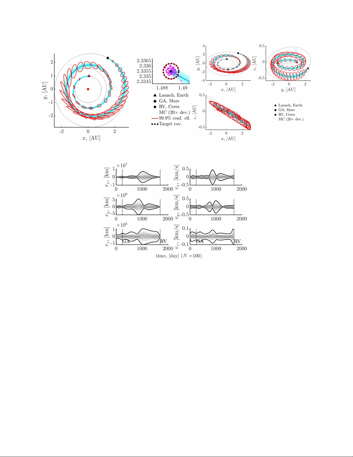
Con v ex Blo c k-Cholesky Approac h to Risk-Constrained Lo w-thrust T ra jectory Design under Op erational Uncertain t y Kenshiro Oguri ∗ and Gregory Lan toine † Abstract Designing robust tra jectories under uncertain ties is an emerging technology that may rep- resen t a k ey paradigm shift in space mission design. As w e pursue more am bitious scien tiﬁc goals (e.g., multi-moon tours, missions with extensiv e comp onen ts of autonom y), it b ecomes more crucial that missions are designed with na vigation (Nav) processes in mind. The eﬀect of Na v pro cesses is statistical b y nature, as they consist of orbit determination (OD) and ﬂigh t- path con trol (FPC). Th us, this mission design paradigm calls for techniques that appropriately quan tify statistical eﬀects of Nav, ev aluate associated risks, and design missions that ensure suf- ﬁcien tly low risk while minimizing a statistical p erformance metric; a common metric is ∆V99: w orst-case (99%-quantile) ∆V exp enditure including statistical FPC eﬀorts. In resp onse to the need, this pap er develops an algorithm for risk-constrained tra jectory optimization under op er- ational uncertainties due to initial state disp ersion, navigation error, maneuver execution error, and imp erfect dynamics mo deling. W e formulate it as a nonlinear stochastic optimal control problem and develop a computationally tractable algorithm that combines optimal cov ariance steering and sequential con vex programming (SCP). Sp eciﬁcally , the prop osed algorithm tak es a blo c k-Cholesky approach for conv ex formulation of optimal cov ariance steering, and leverages a recen t SCP algorithm, SCvx* , for reliable n umerical con vergence. W e apply the developed algorithm to risk-constrained, statistical tra jectory optimization for exploration of dwarf planet Ceres with a Mars gravit y assist, and demonstrate the robustness of the statistically-optimal tra jectory and FPC p olicies via nonlinear Monte Carlo simulation. 1 In tro duction Designing robust tra jectories under uncertainties is an emerging technology that ma y represent a k ey paradigm shift in space mission design. As the complexity of space missions grows to pursue more am bitious scien tiﬁc goals (e.g., multi-moon tours, missions with extensive comp onen ts of au- tonom y), it becomes increasingly crucial that missions are designed with navigation (Na v) processes in mind. The eﬀect of Na v pro cesses is statistical by nature, as they consist of orbit determination (OD) and ﬂight-path control (FPC); FPC is a pro cess that calculates tra jectory correction maneu- v ers (TCMs) based on deliv ered OD solutions. 1 An y risks (e.g., collision with a planetary b ody during a close ﬂyb y) under these statistical eﬀects m ust b e appropriately quan tiﬁed and mitigated ∗ Assistan t Professor, School of Aeronautics and Astronautics, Purdue Univ ersity , W est Lafay ette, Indiana, 47907 † Group Sup ervisor, Outer Planet Mission Design Group, Mission Design and Navigation Section, Jet Propulsion Lab oratory , California Institute of T echnology , Pasadena, California 91109. An earlier version of this pap er was presented as pap er 22-708 at the 2022 AAS/AIAA Astrodynamics Sp ecialist Conference, Charlotte, NC, August 2022. 1 W e are a ware that there are diﬀerent interpretations/de ﬁnitions of “na vigation”; it sometimes refers to only estimation pro cess (i.e., OD) while FPC is considered a “guidance” pro cess. In this pap er, w e tak e the deﬁnition t ypically used at JPL, where Nav encompasses OD and FPC. 1 in mission design pro cesses to ensure the mission safet y . Although these risks hav e been histori- cally mitigated in a rather heuristic manner (e.g., heuristic margins to constrain ts, manually-tuned forced coasting arcs) [ 1 , 2 ], there has b een a growing n umber of studies on directly incorp orating these statistical eﬀects into mission design and thereb y coupling the tra jectory optimization with Na v pro cesses within the design pro cess. Similar to conv entional deterministic problems, existing approac hes to statistical tra jectory optimization under uncertain ties can b e categorized into: indirect metho ds [ 3 , 4 , 5 ], direct metho ds [ 6 , 7 , 8 , 9 , 10 , 11 ] and diﬀeren tial dynamic programming (DDP) [ 12 , 13 ]. This list of papers are certainly not exhaustiv e, but it already highligh ts the growing in terest on this topic in the space mission design communit y . See [ 11 ] and its earlier v ersion [ 14 ] for further discussion that compares these diﬀerent metho ds. Key enablers of these tec hniques lie in the recen t adv ances in sto chastic optimal con trol and optimization communities, particularly in optimal c ovarianc e ste ering [ 15 , 16 , 17 , 18 , 19 , 20 , 21 ] and c omputational c ontr ol based on conv ex programming [ 22 , 23 , 24 , 25 , 26 ], and their application to aerospace problems [ 27 , 28 , 29 , 30 , 31 , 32 ]. Unlik e traditional optimal control, optimal co v ariance steering consider con trolling the mean and co v ariance of the system’s state while minimizing a statistical cost, which dep ends on b oth the state mean and cov ariance; it often also in volv es statistical constrain ts kno wn as chanc e c onstr aints (or equiv alently , risk c onstr aints ), whic h imp oses constraints on probability that constraints b e satisﬁed under state uncertainties. Either explicitly or implicitly , many existing techniques for tra jectory optimization under uncertain ties build on the concept of optimal cov ariance steering, solv ed b y indirect metho ds, direct metho ds, or DDP . A particularly imp ortan t asp ect to consider when developing an algorithm for tra jectory opti- mization under uncertaint y is, what sp e ciﬁc appr o ach we cho ose to formulate the optimal c ovarianc e ste ering pr oblem . First introduced in 1980s by Hotz and Sk elton [ 33 ], the theory of optimal co- v ariance steering has seen rapid adv ances in the sto c hastic optimal con trol communit y in recent y ears, including contin uous-time cov ariance steering [ 16 ] and discrete-time co v ariance steering with c hance constrain ts [ 15 ]. Discrete-time cov ariance steering ma y ﬁnd more relev ant applications in aerospace, considering the nature of discrete opp ortunities for control commands and measuremen ts. It is therefore b eneﬁcial to further discuss some v ariants of discrete-time co v ariance steering, such as one with input constrain ts [ 34 ], one without the need for history feedback [ 17 ], one with output feedbac k [ 18 ], and output-feedback co v ariance steering without history feedback [ 19 ]. In particular, this output-fe e db ack co v ariance steering holds the key to unlo c king the p oten tial of incorp orating the OD pro cess (i.e., taking measuremen ts and applying ﬁltering to estimate the spacecraft or- bit) into the framework of tra jectory optimization under uncertainties. Notably , the discrete-time co v ariance steering studies mentioned in this paragraph formulate the problem in con vex form b y forming a large blo c k-matrix for the system equation and utilizing the Cholesky factor of cov ariance matrices. This class of approac hes are called blo ck-Cholesky formulation in this pap er. An imp ortan t cav eat of the blo ck-Cholesky formulation lies in its computational complexity . As discussed in [ 21 , 8 , 11 ], their computational complexit y is roughly prop ortional to ( n x N 2 ), where n x is the size of the state vector and N is the n um b er of discretized tra jectory segmen ts. Hence, recent studies ha ve developed a more computationally-eﬃcien t formulation of discrete-time co v ariance steering [ 20 ] and its output-feedback v arian t [ 21 ], which ha ve b een successfully applied to robust space tra jectory optimization under uncertain ties [ 9 , 14 , 11 ]. These approac hes propagate the full cov ariance (rather than its Cholesky factor) and do not rely on the blo c k-matrix formulation, and hence called ful l-c ovarianc e formulation in this paper. The main innov ation of these studies lies in its elegant lossless conv exiﬁcation of originally non-conv ex cov ariance propagation equations b y using the Sch ur complemen t and the Karush-Kuhn-T uc ker (KKT) conditions. As a result, the ful l-c ovarianc e formulation enables us to form ulate the discrete-time co v ariance steering problem 2 in con vex form, with its computational complexity roughly proportional to N ( n x + n u ), where n u is the size of the control vector. This implies that the full-cov ariance formulations is more b eneﬁcial for larger tra jectory optimization problems (i.e., greater N ). Although the full-co v ariance approach has a key adv antage o ver blo ck-Cholesky approaches in terms of the computational complexit y , they also hav e critical drawbac ks that w arran t careful considerations for space tra jectory optimization. The drawbac ks are: (1) n umerical ill-conditioning, (2) non-conv ex chance constraints, and (3) inﬂexible cost functions. The ﬁrst p oin t, numerical ill- conditioning, is related to the large scale diﬀerences that are inherent to space tra jectories, esp ecially in interplanetary tra jectories. T o illustrate this aspect, let us consider spacecraft on a tra jectory from Mars to a main-b elt asteroid with state uncertain ty of 10 km in p osition and 1 m/s in velocity (standard deviation). While the magnitudes of these p osition/v elo cit y uncertaint y v ariances are of { 100 km 2 , 1 × 10 − 6 km 2 / s 2 } , the magnitude of p osition v ector measured from Sun is in the order of ∼ 2 − 4 × 10 8 km; this implies that the numerical solver would need to deal with a problem of condition num b er as large as ∼ 1 × 10 14 and may not b e as reliable as desired. 2 In fact, this type of numerical ill-conditioning is the main motiv ation for square-ro ot form ulations of OD ﬁlters (e.g., square-ro ot unscen ted Kalman ﬁlter [ 35 ] and square-ro ot information ﬁlter [ 36 ]), which can recov er up to a half of the digits of precision that would hav e b een lost otherwise. The second drawbac k, non-conv e x c hance constraints, is due to the use of full cov ariance matrices as decision v ariables. As demonstrated in existing studies on chance-constrained control [ 15 , 17 , 18 , 19 , 30 , 31 ], we can formulate man y c hance constrain ts in con vex form if the Cholesky factor of co v ariance matrices are decision v ariables. On the other hand, full-cov ariance approac hes directly handle cov ariance matrices, whic h is a nonlinear function of the Cholesky factor, hence making those c hance constrain ts non-conv ex, including con trol magnitude c hance constrain ts and half-plane state c hance constraints, to name a few. This fact requires us to approximate chance constraints at each iteration via either linearization [ 9 , 14 , 11 ] or con vex-conca v e pro cedure [ 21 ]. Lastly , the issue of inﬂexible cost functions arises from the lossless conv exiﬁcation pro cess in the form ulation of full-cov ariance approaches. The lossless prop ert y , which is crucial for conv ex- ifying the full cov ariance propagation equation, relies on the KKT conditions, in particular their complemen tary slackness condition. T o meet the KKT conditions, [ 20 , 21 ] assume a sp eciﬁc form of ob jective function, and it is sho wn [ 37 ] that their full-cov ariance approaches cannot consider the ∆V99 cost metric (99%-quantile ∆V, representing w orst-case ∆V under statistical FPC), which is a t ypical cost in space mission design. [ 11 ] prop oses a middle-ground solution that relaxes the inﬂexibilit y and enables appro ximate formulation of the ∆V99 cost. Giv en these observ ations, this pap er dev elops an approac h based on block-Cholesky formulation for robust tra jectory optimization under uncertain ties. 3 Main con tributions of the presen t pap er are threefold. First, this pap er leverages a recen t form ulation of blo c k-Cholesky output-feedbac k co v ariance steering [ 30 ] and a sequential con vex programming (SCP) algorithm SCvx* [ 26 ] to develop an optimization algorithm for risk-constrained low-thrust tra jectory design under uncertain ties. The algorithm incorporates v arious op erational uncertain ties due to na vigation errors, maneuver execution errors, initial state disp ersion, and imp erfect dynamics mo deling. Second, we extend the dev elop ed algorithm to incorp orate planetary gravit y assists (GAs), which is a m ust-hav e option in any mo dern interplanetary mission design. In particular, we utilize the patched-conic GA mo del in this study . Third, the dev elop ed algorithm introduces some improv emen ts in its mathematical 2 If we normalize the problem to make both 1 AU and 1 µ sun equal to unity , the condition num b er might become ev en worse. In the case of the example ab o ve, the v ariances of p osition and velocity b ecome approximately { 4 . 4 × 10 − 15 , 1 . 1 × 10 − 17 } against 2-3 AU. 3 A recent pap er of the ﬁrst author of this pap er develops an algorithm based on a full-cov ariance approach [ 11 ], if the readers are interested in the other formulation too. 3 form ulation, including: a more general class of augmen ted Lagrangian functions than introduced in the original SCvx* pap er [ 26 ], which can smo othly appro ximate the l 1 -p enalt y function for b etter con vergence; and a formulation of three-dimensional control magnitude chance constraints that pro vide tighter approximation than existing studies [ 7 , 9 , 38 , 13 ] and are rigorously conserv ativ e compared to a heuristic approach taken in [ 12 ]. See Fig. 1 for a conceptual illustration of the prop osed approach. The rest of the pap er is structured as follows. After Section 2 in tro duces the system equation, Section 3 details the sto c hastic optimal control form ulation that incorp orates op erational uncer- tain ties and statistical risk constrain ts. Section 4 presents a tractable conv ex approximation of the sto c hastic optimal control problem based on a blo ck-Cholesky approach, which simultaneously optimizes the reference tra jectory and FPC policies under the Kalman ﬁlter process and linear FPC p olicies. Section 5 dev elops a SCP algorithm that lev erages the algorithmic framew ork of SCvx* and iterativ ely solv es the con v ex subproblem to march tow ard an optimal solution. Section 6 applies the developed algorithm to robust tra jectory optimization for exploration of dwarf planet Ceres with a Mars gravit y assist, and demonstrates the robustness of the obtained statistically-optimal tra jectory and asso ciated FPC p olicies via nonlinear Monte Carlo sim ulation. 2 Equations of Motion This pap er considers low-thrust spacecraft orbital motions with a simpliﬁed low-thrust mo del that ignores the mass decrease due to thrusting. This assumption is in line with most of the existing approac hes to robust s pace tra jectory optimization under uncertaint y , including [ 7 , 12 , 9 , 4 ]. While some studies, suc h as [ 8 , 39 , 10 ], consider the mass ﬂow equation and associated uncertain ty , they also p oin t out that the resulting distribution of the mass uncertaint y b ecomes highly non- Gaussian and in fact tak e the form of generalized c hi-squared distribution. It is w ell-kno wn that the generalized chi-squared distribution does not ha ve closed-form expression for the probability density function, making rigorous characterization of mass uncertain ty less straightforw ard. Developing an approac h to prop erly incorporating the eﬀect of mass uncertain ty is an imp ortant direction of future w ork. Th us, letting x ∈ R n x denote the orbital state (e .g., p osition/v elo cit y , osculating orbital ele- men ts, etc) and u ∈ R 3 b e the con trol acceleration due to the low-thrust engine, we can express the equations of motion in a generic form as follows: ˙ x = f ( x , u , t ) = f 0 ( x , t ) + F ( x ) u (1) where f 0 ( · , · ) : R n x × R 7→ R n x represen ts natural orbital dynamics; F ( · ) : R n x 7→ R n x × 3 returns a matrix that maps the acceleration to the rate of the state change. Eq. ( 1 ) encompasses equations of motion describing low-thrust orbital dynamics in v arious co ordinate systems. Sp eciﬁcally , this study uses the Cartesian co ordinate system to express the system state and considers perturb ed tw o-b ody dynamics. Then, the orbital state and the dynamics functions are giv en by: x =  r v  , f 0 ( x , t ) = " v − µ ∥ r ∥ 3 2 r + a pert ( x , t ) # , F =  0 3 × 3 I 3  (2) where r ∈ R 3 and v ∈ R 3 are the spacecraft p osition and v elo cit y in Cartesian coordinates, resp ectiv ely; µ is the gra vitational parameter of the central b ody; a pert ( x , t ) is the p erturbing acceleration. 4 Statistical T rajectory Optimization Algorithm Va l i d a t i o n input output Dynamics Model Uncertainty Model Environment Model Data / Results Robust Mission Computational Process • Nom i n a l co n t r o l • FPC par am et er • Reference T rajectory • State statistics under OD & FPC UQ with Nav (O D+FPC ) Decision variable update via mathematical programming *UQ: uncertainty quantification, F PC: flight-path control Decision variables Mission Model Performance Index Mission Constraints Nav modeling (e.g., OD & FPC frequency) Monte Carlo Figure 1: F undamental idea of statistical tra jectory optimization under uncertain ty 3 Risk-Constrained Nonlinear Sto c hastic Optimal Con trol Prob- lem Fig. 1 presents the fundamen tal idea b ehind the prop osed formulation for risk-constrained tra jec- tory optimization under uncertain ties. The form ulation directly incorp orates op erational uncer- tain ty models (e.g., measurement function, measurement noise, OD frequency) as well as statistical risk constrain ts (e.g., safety with 99.9% conﬁdence) while minimizing the t ypical statistical cost, ∆V99. Considering other statistical costs is straigh tforward due to the ﬂexibility of block-Cholesky approac hes as opp osed to full-co v ariance approaches. The developed algorithm then solves for sta- tistically optimal lo w-thrust tra jectories under the modeled uncertainties b y utilizing the mean and co v ariance information derived from the Kalman ﬁlter pro cess, and simultaneously optimizing the reference tra jectory and FPC p olicies via SCP . This section formulates the problem of risk-constrained low-thrust tra jectory optimization under uncertain ty in a form of chance-constrained optimal control. Our formulation incorp orates the inﬂuence of ma jor uncertain errors in space missions (initial state disp ersion, maneuver execution error, and OD error) as well as the corrective eﬀect of FPC eﬀorts. 3.1 Nonlinear Sto c hastic System 3.1.1 Initial State Disp ersion An y space tra jectories b egin with initial state disp ersion, such as due to launch disp ersion and orbit insertion errors. W e mo del such initial state disp ersion via a Gaussian distribution as: x 0 ∼ N ( x 0 , P 0 ) (3) 3.1.2 Maneuv er Execution Error An y maneuvers in volv e some errors that are uncertain by nature, due to thruster misalignmen t, o ver/under burn, among other causes. A common approac h to modeling suc h errors is the Gates 5 mo del [ 40 ], which captures the error that is prop ortional to the applied thrust commands as well as that is ﬁxed irresp ectiv e of the commands. Using the Gates mo del, for a given commanded con trol u , a maneuver execution error, denoted b y e u , is given as [ 29 ]: e u = G exe ( u ) w exe , G exe ( u ) = T ( u ) P 1 / 2 gates ( u ) , w exe ∼ N (0 , I 3 ) , (4) where w exe are indep enden t and identically distributed (i.i.d.) standard Gaussian v ectors, i.e., E [ w exe ] = 0 and E  w exe ( t i ) w exe ( t j ) ⊤  = δ i,j I , where δ i,j is the Kroneck er delta. P gates ( · ) denotes the execution error cov ariance in the local co ordinates that are deﬁned with resp ect to the thrust direction while T ( · ) rotates the direction to the co ordinates we propagate our system, given by P gates ( · ) = diag( σ 2 p , σ 2 p , σ 2 m ) , T ( · ) =  ˆ S ˆ E ˆ Z  , ˆ Z = u ∥ u ∥ 2 , ˆ E = [0 , 0 , 1] ⊤ × ˆ Z    [0 , 0 , 1] ⊤ × ˆ Z    2 , ˆ S = ˆ E × ˆ Z (5) Here, σ 2 p = σ 2 3 + σ 2 4 ∥ u ∥ 2 2 and σ 2 m = σ 2 1 + σ 2 2 ∥ u ∥ 2 2 , where { σ 1 , σ 2 } are { ﬁxed, prop ortional } magnitude errors while { σ 3 , σ 4 } are { ﬁxed, proportional } p oin ting errors. It is clear that the terms σ 2 2 ∥ u ∥ 2 2 and σ 2 4 ∥ u ∥ 2 2 tak e greater v alues for larger control command, and hence represent prop ortional errors. 3.1.3 Stochastic Diﬀerential Equations T o incorp orate uncertain errors and FPCs in our mission design pro cess, one of the most straight- forw ard approaches is to express our system via nonlinear sto c hastic diﬀerential equations (SDEs). Based on the equations of motion Eq. ( 1 ), our sto c hastic system can b e formally expressed via a set of nonlinear SDEs as: d x =[ f ( x , u , t ) + F ( x ) e u ]d t + G ( x )d w ( t ) , (6) where G ( · ) : R n x 7→ R n x × n w represen ts the in tensity of disturbances, mapping d w ( t ) to the random v ariation of the state; d w ( t ) : R 7→ R n w is a standard Brownian motion vector, i.e., E [d w ] = 0 and E  d w ( t )d w ⊤ ( t )  = I d t . The form G ( · )d w encompasses v arious t yp es of disturbances, including unmo deled external p erturbations (e.g., solar radiation pressure, momen tum de-saturation opera- tions, etc). The term F ( x ) e u captures the eﬀect of maneuv er execution errors to the v ariation of state uncertain ty . 3.2 Nonlinear Sto c hastic System with Na vigation Uncertaint y Let us then mo del the Na v pro cesses (OD and FPC). W e mo del the FPC p olicy suc h that c alcu- lates tra jectory corrections based on imp erfect state knowledge giv en by orbit determination (OD) pro cesses. 3.2.1 Orbit Determination Mo del W e mo del the OD pro cess as a sequence of ﬁltering pro cesses with discrete-time observ ations. Assuming that a set of spacecraft tracking data b ecomes av ailable at time t k , the observ ation pro cess is giv en by: y k = f obs ( x k , t k ) + G obs ( x k ) w obs ,k , k = 0 , 1 , ..., N (7) 6 where y k ∈ R n y are the (collection of ) measuremen ts; f obs ( · , · ) : R n x × R 7→ R n y and G obs ( · ) : R n x 7→ R n y × n y mo del the observ ation process. w obs ,k ∈ R n y is measurement noise, mo deled as a sequence of i.i.d. standard Gaussian random v ectors. A t time t k , the OD solution, ˆ x k , is obtained by a ﬁltering pro cess with the past observ ations y i ( i = 0 , 1 , ..., k ) as follo ws: ˆ x k = F k ( ˆ x − 0 , y i : i = 0 , 1 , ..., k ) , (8) where the “ − ” sup erscript indicates a quantit y righ t b efore the measuremen t up date; ˆ x − 0 denotes the initial state estimate. Filtering typically utilizes the inno v ation pro cess e y − k , deﬁned as: e y − k = y k − f obs ( ˆ x − k ) . (9) 3.2.2 Fligh t-path Con trol Mo del Fligh t-path controls are a collection of eﬀorts that drive the orbital state deviation back to the nominal tra jectory , planed based on imperfect OD solutions. Hence, this study mo dels FPCs o ver the course of a tra jectory b y a sequence of feedbac k policies that compute necessary control mo diﬁcations based on the curren t state estimate given by Eq. ( 8 ). The feedback p olicies are thus expressed as: u k = π k ( ˆ x k , Ω k ) , (10) where Ω k denotes a set of parameters used to compute the corrective controls u k according to the p olicy π k . 3.3 Original Problem 3.3.1 Statistical Cost Metric A common cost function in space tra jectory optimization is the total control eﬀort. How ever, we ma y not directly minimize the con trol eﬀort in sto c hastic setting b ecause it is not w ell-deﬁned due to the sto c hasticity of u under the feedbac k p olicy Eq. ( 10 ). Thus, this study considers minimizing the p -quan tile of the closed-lo op control eﬀort, i.e., J = Z t f t 0 Q X ∼∥ u ∥ 2 ( p ) (11) where Q X ( p ) is the quan tile function of a random v ariable X ev aluated at probability p , formally deﬁned as: Q X ( p ) = min { x ∈ R | P [ X ≤ x ] ≥ p } . (12) Note that using p = 0 . 99 corresp onds to minimizing 99%-quantile of con trol cost, i.e., ∆V99. 3.3.2 Risk Constraints The constraints considered in this study include path constrain ts and terminal constraints. As our state and control are sub ject to uncertain ty , those constraints are not deterministic an ymore and need to b e treated sto c hastically . In particular, we consider a class of probabilistic constraints called chanc e c onstr aints to formu- late our path constrain ts, as they naturally represen t stochastic analogs of deterministic constraints 7 classically considered in mission design. Intuitiv ely , a chance constraint imp oses a bound on the probabilit y that a particular constrain t b e satisﬁed (i.e., no collision with an obstacle with a prob- abilit y greater than 99 . 9%); see, for instance, [ 29 , 41 , 42 , 5 , 14 ] and references therein, for the use of c hance constraints in the context of space tra jectory optimization. Mathematically , path chance constraints imp osed on discrete-time state and control are ex- pressed as: P [ c j ( x , u , t ) ≤ 0] ≥ 1 − ε j , (13) where P [ · ] denotes the probability op erator, c j ( · ) : R n x × R 3 × R 7→ R represents the j -th nonlinear constrain t function, and ε j is a risk b ound asso ciated with the j -th constraint (e.g., ε j = 0 . 001 for 99 . 9% conﬁdence). This imp oses the constraint c j ≤ 0 to b e satisﬁed with probability greater than or equal to 1 − ε j . Similarly , we mo del the terminal constraints as distributional constraints that ensure that the ﬁnal state is within a prescrib ed region. Sp eciﬁcally , w e imp ose terminal constraints on the ﬁnal state, x N , to ac hiev e the target x f on a v erage with prescribed accuracy represen ted b y the ﬁnal co v ariance P f : E [ x N ] − x f = 0 , (14a) Co v [ x N ] ⪯ P f (14b) where E [ · ] and Cov [ · ] denotes the exp ectation and cov ariance op erators, resp ectiv ely . Mathemat- ically , E [ x ] = R x p ( x )d x where p ( x ) is a probability density function (p df ) of x , and Co v [ x ] = E  ( x − E [ x ])( x − E [ x ]) ⊤  . Th us, letting Θ represen t a vector of relev an t parameters to optimize (whic h take diﬀerent forms dep ending on sp eciﬁc problems), our original problem can b e expressed as in Problem 1 . Problem 1 (Original problem) . Find x ∗ ( t ) π k , ∀ k , and Θ that minimize the c ost Eq. ( 11 ) subje ct to the dynamic al c onstr aint Eq. ( 6 ) , p ath chanc e c onstr aints Eq. ( 13 ) , and terminal c onstr aint Eq. ( 14b ) under a se quenc e of FPCs determine d by Eq. ( 10 ) with the state estimates Eq. ( 8 ) b ase d on observations Eq. ( 7 ) . 4 T ractable F orm ulation via blo c k-Cholesky Co v ariance Steering In general, Problem 1 is in tractable to solve. A ma jor b ottlenec k of the diﬃculty lies in the pro cess of unc ertainty quantiﬁc ation (UQ) to ev aluate the statistics of the state, cost, and constrain ts under uncertaint y , which is computationally exp ensiv e in general, except for some sp ecial cases. In nonlinear tra jectory optimization, it is most likely the case that we m ust iteratively p erform suc h exp ensiv e UQ pro cesses to ev aluate the functions and their gradients with resp ect to decision v ariables. This requires an eﬃcient and reliable solution metho d. Among multiple p ossible approaches, this study prop oses a solution metho d based on optimal co v ariance steering and sequential con v ex programming (SCP) to solve our problem. The prop osed approac h appro ximately form ulates the originally in tractable stochastic problem in a conv ex, de- terministic form at eac h successiv e iteration; in particular, we emplo y a block-Cholesky form ulation as discussed in Section 1 . At eac h iteration, the original problem is approximated as a conv ex sub- problem, whic h is solved with guaran teed conv ergence to the global optimum of the appro ximated problem due to the conv ex prop ert y . Once the conv ergence of a con vex subproblem is ac hieved, then the subproblem solution is used as a new reference tra jectory for the next iteration. Leverag- ing the reliabilit y and eﬃciency of con vex programming, this solution metho d pro vides us with a 8 v ehicle for o vercoming the ma jor b ottlenec k of numerical solutions to nonlinear sto c hastic optimal con trol problems, at the cost of appro ximate dynamical evolution of the sto chastic state deviations from the reference tra jectory . Note that the dynamical feasibilit y of the reference tra jectory is not compromised in our solution metho d, and the designed reference tra jectory satisﬁes the nonlinear dynamics up to the user-sp eciﬁed tolerance. Let us ﬁrst approximately reformulate Problem 1 in a deterministic, conv ex form in the follow- ing. 4.1 Linear State Statistics Dynamics T o obtain the con vex subproblem, Eq. ( 6 ) is ﬁrst linearized and discretized assuming ﬁxed-time problems (i.e., t 0 and t f not part of optimization v ariables). It is p ossible to extend the formulation presen ted in this article to v ariable-time problems by incorp orating the adaptiv e-mesh mechanism [ 43 ]. Such an extension is left as exciting future work, as it w ould allow the FPC p olicies (which are b eing optimized) to adjust maneuver ep o c hs based on OD solutions. 4.1.1 Linear, Discrete-time System The initial a priori state estimate ˆ x − 0 and its error e x − 0 (e.g., state disp ersion estimate immediately after deplo yment from a launcher) are assumed to b e Gaussian-distributed, i.e., ˆ x − 0 ∼ N ( x 0 , ˆ P − 0 ) and e x − 0 ∼ N (0 , e P − 0 ), where ( · ) indicates the mean of a random v ariable. It implies that the initial state x − 0 is distributed as x 0 = ˆ x − 0 + e x − 0 ∼ N ( x 0 , ˆ P − 0 + e P − 0 ). Linearizing the system Eq. ( 6 ) and discretizing the time into in terv als t 0 < t 1 < t 2 < ... < t N = t f with zeroth-order-hold (ZoH) con trol, i.e., u ( t ) = u k , ∀ t ∈ [ t k , t k +1 ), yields [ 44 , 30 ]: x k +1 = A k x k + B k u k + c k + G exe ,k w exe ,k + G k w k , k = 0 , 1 , ..., N − 1 (15) where A k , B k , c k , and G k represen t linear system matrices that are obtained b y linearizing ab out the reference state x ref ( t ) and control u ref ( t ) and discretizing the system in time (see Ref. [ 30 ] for the deﬁnition); w k is an i.i.d. standard Gaussian random v ector. 4.1.2 Filtered State Dynamics Since the state is initially Gaussian-distributed and ob eys the linear dynamics in a con vex subprob- lem, the optimal, unbiased state estimate can b e obtained by the Kalman ﬁlter. Th us, the ﬁltering pro cess Eq. ( 8 ) is giv en as: ( ˆ x − k = A k − 1 ˆ x k − 1 + B k − 1 u k − 1 + c k − 1 e P − k = A k − 1 e P k − 1 A ⊤ k − 1 + G exe ,k − 1 G ⊤ exe ,k − 1 + G k − 1 G ⊤ k − 1 (time up date) ( ˆ x k = ˆ x − k + L k ( y k − C k ˆ x − k ) e P k = ( I − L k C k ) e P − k ( I − L k C k ) ⊤ + L k D k D ⊤ k L ⊤ k , (measuremen t up date) (16) where e P k denotes the estimate error cov ariance; L k is the Kalman gain; C k and D k are the linearized measuremen t equation ab out the reference, given b y e P k ≜ Co v [ e x k ] , L k ≜ e P − k C ⊤ k ( C k e P − k C ⊤ k + D k D ⊤ k ) − 1 , C k ≜ ∂ f obs ∂ x ( x ref k ) , D k = G obs ( x ref k ) (17) 9 As classically known in estimation theory , e P k and L k can b e computed a priori for linear systems. Com bining the t wo equations in Eq. ( 16 ), the ﬁltered state pro cess under sto chastic error and Kalman ﬁltering is written as: ˆ x k +1 = A k ˆ x k + B k u k + c k + L k +1 e y − k +1 (18) where e y − k is the inno v ation pro cess Eq. ( 9 ), whose linear form and its cov ariance, denoted by P e y − k , are giv en as [ 30 ] e y − k = C k e x k + D k w obs ,k , P e y − k ≜ Co v  e y − k  = C k e P − k C ⊤ k + D k D ⊤ k . (19) 4.1.3 Linear Flight-path Con trol Mo del W e consider a linear FPC p olicy to mo del Eq. ( 10 ) for conv ex form ulation. In particular, w e use the follo wing form of the control p olicy: u k = u k + K k z k , (20) where u k is a nominal control input, K k is a feedback gain matrix, and z k is a sto chastic pro cess giv en by z k +1 = A k z k + L k +1 e y − k +1 , z 0 = ˆ x 0 − x 0 . (21) 4.1.4 State and Con trol Statistics W e are now ready to analytically express the statistics of the state and con trol—in particular, their ﬁrst and second statistical moments, i.e., mean and co v ariance. As derived in Ref. [ 30 ], it is con venien t to express Eq. ( 18 ) in a blo c k-matrix form as:      ˆ x 0 ˆ x 1 ˆ x 2 . . .      =      I n x A 0 A 1 A 0 . . .      ˆ x − 0 +      0 0 B 0 0 A 1 B 0 B 1 . . .           u 0 u 1 u 2 . . .      +      0 0 I n x 0 A 1 I n x . . .           c 0 c 1 c 2 . . .      +      L 0 0 A 0 L 0 L 1 A 1 A 0 L 0 A 1 L 1 . . .           e y − 0 e y − 1 e y − 2 . . .      (22) whic h can b e expressed in a compact form as: ˆ X = A ˆ x − 0 + B U + C + L Y , (23) where ˆ X = [ ˆ x ⊤ 0 , ˆ x ⊤ 1 , ..., ˆ x ⊤ N ] ⊤ , U = [ u ⊤ 0 , u ⊤ 1 , ..., u ⊤ N − 1 ] ⊤ , Y = [ e y − 1 ⊤ 0 , e y − 1 ⊤ 1 , ..., e y − 1 ⊤ N ] ⊤ , and A , B , C , L are deﬁned accordingly . Similarly , deﬁne K to contain K k in a blo c k matrix form as in Ref. [ 30 ]. Let us also deﬁne matrices E x k and E u k to extract x k and u k from X and U , resp ectively , as x k = E x k X and u k = E u k U . Then, the mean and cov ariance of the state are deriv ed in Ref. [ 30 ], summarized as follows: x k = E x k ( A x 0 + B U + C ) , (mean) P k = ˆ P k + e P k , (total co v ariance) ˆ P k = E x k ( I + BK ) S ( I + BK ) ⊤ E ⊤ x k , (state disp ersion co v ariance) P u k = E u k KSK ⊤ E ⊤ u k (con trol cov ariance) (24) 10 where recall that e P k is the OD cov ariance and recursiv ely calculated according to the Kalman ﬁlter as in Eq. ( 16 ). S is a term that is indep enden t from the con trol v ariables, giv en by S = A ˆ P 0 − A ⊤ + LP Y L ⊤ . (25) In our form ulation, a Cholesky square-ro ot form of cov ariance matrices is conv enient due to its con vex prop ert y . Such square-ro ot forms of co v ariance matrices are given as follows: P 1 / 2 k = h ˆ P 1 / 2 k e P 1 / 2 k i , ˆ P 1 / 2 k = E x k ( I + BK ) S 1 / 2 , P 1 / 2 u k = E u k KS 1 / 2 , S 1 / 2 = h A ˆ P 1 / 2 0 − LP 1 / 2 Y i (26) Remark 1. As cle ar fr om Eqs. ( 24 ) and ( 26 ) , x k , P 1 / 2 k , ˆ P 1 / 2 k , and P 1 / 2 u k ar e aﬃne in the FPC vari- ables u k and K k (se e Pr op osition 1 of R ef. [ 30 ]), which plays a key r ole in our c onvex formulation. 4.2 Cost F unction Under ZoH control input u ( t ) = u k , ∀ t ∈ [ t k , t k +1 ), Eq. ( 11 ) is equiv alen t to J = N − 1 X k =0 Q X ∼∥ u k ∥ 2 ( p )∆ t k , ∆ t k = t k +1 − t k (27) Applying Lemma 4 of Ref. [ 30 ], w e can calculate the upp er b ound of Eq. ( 27 ) as follo ws: J ≤ J ub = X k h ∥ u k ∥ 2 + m χ 2 (1 − p, n u )    P 1 / 2 u k    2 i ∆ t k (28) where m χ 2 ( ε, n u ) is the square ro ot of the quan tile function of the chi-squared distribution with n u degrees of freedom, ev aluated at probability (1 − ε ), and is mathematically expressed as: m χ 2 ( ε, n u ) = q Q X ∼ χ 2 ( n u ) (1 − ε ) (29) Imp ortan tly , Eq. ( 28 ) is conv ex in U and K due to Remark 1 . W e minimize the upp er b ound J ub instead of J directly . m χ 2 ( ε, n u ) is straigh tforward to calculate in modern programming lan- guages. W e can calculate m χ 2 ( ε, n u ) via p chi2inv (1 − ε, n u ) in Matlab and p chi2 . cdf (1 − ε, n u ) in scipy . 4.3 Constrain t F unction T ractable form ulation of Eq. ( 13 ) dep ends on the sp eciﬁc form of constraints of in terest. In this article, we consider three imp ortan t constrain ts that are common in in terplanetary low-thrust tra jectory design: thrust magnitude c onstr aint , terminal c onstr aints , and planetary gr avity assist c onstr aint . 4.3.1 Thrust Magnitude Chance Constraints: With a risk tolerance ε u and maxim um thrust acceleration u max > 0, the thrust magnitude con- strain t is expressed as a chance constraint as: P [ ∥ u k ∥ 2 ≤ u max ] ≥ 1 − ε u , k = 0 , 1 , ..., N − 1 (30) 11 T able 1: Magnitude constraint tightness comparison Approac h { ε, n u } = { 10 − 2 , 3 } { 10 − 3 , 3 } { 10 − 2 , 4 } { 10 − 3 , 4 } Prop osed [Eq. ( 29 )] m χ 2 = 3 . 3682 4 . 0331 3 . 6437 4 . 2973 Previous [ 7 ] [Eq. ( 32 )] m χ 2 (old) = 4 . 7669 5 . 4490 5 . 0349 5 . 7169 Since Eq. ( 30 ) is a sp ecial form of Eq. 53 in Ref. [ 30 ], we can directly apply Lemma 3 of Ref. [ 30 ] to Eq. ( 30 ), yielding ∥ u k ∥ 2 + m χ 2 ( ε u , n u )    P 1 / 2 u k    2 ≤ u max , k = 0 , 1 , ..., N − 1 (31) whic h is again con vex in U and K due to Remark 1 . Note that conv ex form ulation of thrust magnitude chance constrain ts with mass uncertaint y requires more analytical eﬀort; see Ref. [ 8 ] for instance. Remark 2. Contr ol chanc e c onstr aints given by Eq. ( 31 ) pr ovide a b etter appr oximation than the one pr op ose d in Ridderhof et.al.[ 7 ] (and use d in Bene dikter et.al.[ 39 ]). The key diﬀer enc e lies in the deﬁnition of m χ 2 ( ε u , n u ) that app e ar in Eqs. ( 28 ) and ( 31 ) , which is deﬁne d as in Eq. ( 29 ) in this study. On the other hand, the e quivalent of m χ 2 pr op ose d in pr evious studies [ 7 , 39 ] takes the fol lowing form (denoting it as m χ 2 (old) ): m χ 2 (old) =    q 2 ln 1 ε + √ n u ( n u > 2) , q 2 ln 1 ε ( n u = 1 , 2) (32) The values of m χ 2 given by Eq. ( 29 ) (pr op ose d one) and by Eq. ( 32 ) (pr evious one [ 7 , 39 ]) c oincide when n u = 2 , wher e as those by Eq. ( 29 ) ar e smal ler for n u > 2 , le ading to tighter (henc e b etter) c onstr aints. This tighter b ound is p articularly b eneﬁcial in sp ac e applic ations sinc e we typic al ly de al with thr e e-dimensional c ontr ol input (e.g., thrust, ac c eler ation, etc). T able 1 numeric al ly c omp ar es the two appr o aches, c onﬁrming the tightness of our appr oximation. The b eneﬁt of this tighter b ound is not limite d to c ontr ol magnitude c onstr aints but br o ad ly applic able to any magnitude- r elate d chanc e c onstr aints, including state deviation c onstr aints (se e R ef. [ 30 ]). 4.3.2 T erminal Constrain ts A conv ex formulation of Eq. ( 14b ) is readily a v ailable in existing studies (e.g., Refs. [ 18 , 30 ]), yielding: E x N ( A x 0 + B U + C ) − x f = 0 , (33a)    ( P f − e P N ) − 1 / 2 E x N ( I + BK ) S 1 / 2    2 − 1 ≤ 0 . (33b) whic h are conv ex in U and K . 4.4 Incorp orating Planetary Gravit y Assists As commonly done in interplanetary mission design, we use the patched-conic mo del [ 45 ] to mo del the eﬀect of GA on the state tra jectory under uncertain t y and formulate (c hance) constraints accordingly . In this mo del, a GA rotates the spacecraft velocity relative to the planet while the 12 p eriapsis radius ab out the planet, r peri is constrained to b e ab ov e a planetary impact radius, r p min . Note that a higher-ﬁdelity GA mo deling is also p ossible to incorp orate in the prop osed framework. In that case, extending the formulation prop osed in Ref. [ 46 ] to sto c hastic setting would b e a straigh tforward approach, where the state statistics would b e propagated in the planet-centric frame while imp osing the impact constraint. Let a GA o ccur at t k , and assign k and k + 1 to the no des that are immediately before and after the GA, resp ectiv ely . Denoting the spacecraft velocity relativ e to the planet b y v ∞ k = v k − v p ( t k ), where v p ( t k ) is the planet’s velocity at t k , under the patched-conic mo del, the GA eﬀect is instan taneous and rotates v ∞ k b y a turn angle θ [ 45 ], i.e., t k = t k +1 , r k = r k +1 ,   v ∞ k +1   2 = ∥ v ∞ k ∥ 2 , v ∞ k +1 · v ∞ k = ∥ v ∞ k ∥ 2 2 cos θ (34) The periapsis radius with resp ect to the planet during the ﬂyb y , r peri ( · ), is a function of θ and v ∞ k (hence of v k and t k ), and must b e greater than a minimum altitude, r p min , as follows [ 45 ]: r peri ( v k , θ , t k ) ≥ r p min , r peri ( v k , θ , t k ) = µ p   v ∞ k   2 2 1 sin θ 2 − 1 ! , (35) where µ p is the planet’s gravit y constant. T o ease the form ulation in Section 4.4.3 , we equiv alen tly express Eq. ( 35 ) as: ∥ v ∞ k ∥ 2 − v u u t µ p r p min 1 sin θ 2 − 1 ! ≤ 0 (36) 4.4.1 State Statistics Mapping across a Gra vit y Assist While Eq. ( 34 ) is simple to apply for deterministic problems, it is not suited for stochastic problems b ecause it do es not clarify how the state statistics should b e mapp ed across a GA. Th us, this study deriv es another form of Eq. ( 34 ) that furnishes an explicit form ula that maps P k to P k +1 across a GA ev en t. T o this end, w e express the rotation of v ∞ via an orthogonal matrix R GA ∈ R 3 × 3 as v ∞ k +1 = R GA v ∞ k , where R GA is assumed to b e deterministic (hence θ to o) and may b e considered as an optimization v ariable. Ho wev er, using R GA as an optimization v ariable in tro duces another issue; imp osing the orthogonalit y condition is non-conv ex. T o address this issue, this study utilizes Cayley tr ansform 4 to express the orthogonal matrix R GA in terms of a skew-symmetric matrix V ∈ R 3 × 3 (hence V ⊤ = − V ) as R GA = ( I 3 + V ) − 1 ( I 3 − V ), yielding v ∞ k +1 = ( I 3 + V ) − 1 ( I 3 − V ) v ∞ k ⇔ v k +1 − v p ( t k ) = ( I 3 + V ) − 1 ( I 3 − V )[ v k − v p ( t k )] (37) where I n ∈ R n × n is an identit y matrix. It is clear that, because R GA = ( I 3 + V ) − 1 ( I 3 − V ) is a rotation matrix, Eq. ( 37 ) automatically satisﬁes the third constrain t of Eq. ( 34 ). W e can parameterize the skew-symmetric matrix V by only three scalars and express it as V = [ u k ] × with u k ∈ R 3 , where [ · ] × denotes the matrix cross pro duct op erator. Here, we can see u k as a con trol input at t k that c haracterizes the eﬀect of the GA at this ep o c h. This viewp oin t, com bined with the Cayley transformation, allows us to describ e the mapping of state under the eﬀect of a GA as a nonlinear function, whic h then provides a linear mapping equation. This idea is formally stated in Lemma 1 . 4 F or any sk ew-symmetric matrix A , a matrix Q that satisﬁes Q = ( I + A ) − 1 ( I − A ) is an orthogonal matrix with its determinant +1, i.e., QQ ⊤ = I and | Q | = 1. 13 Lemma 1. Using Cayley tr ansformation, the mapping of orbital states x k to x k +1 due to a gr avity assist is expr esse d as a nonline ar function of x k , u k , t k , as fol lows: x k +1 = f GA ( x k , u k , t k ) =  r k v p ( t k ) + R GA ( u k ) · [ v k − v p ( t k )]  , R GA ( u k ) = ( I 3 + [ u k ] × ) − 1 ( I 3 − [ u k ] × ) (38) wher e [ · ] × denotes the matrix cr oss pr o duct op er ator, and ( I 3 + [ u k ] × ) − 1 always exists. Also, its line arize d e quation c an b e expr esse d as x k +1 = A k x k + B k u k + c k , wher e the line ar system matric es A k , B k , c k ar e given by A k = ∂ f GA ∂ x     ref =  I 3 0 3 × 3 0 3 × 3 R GA ( u ref k )  , B k = ∂ f GA ∂ u     ref =  0 3 × 3 ( I 3 + [ u ref k ] × ) − 1 ([ v ref k +1 ] × + [ v ref k ] × − 2[ v p ] × )  , c k = f GA ( x ref k , u ref k ) − A k x ref k − B k u ref k (39) Pr o of. See Section A.1 . Using Lemma 1 , w e can in tegrate the eﬀect of GAs in to the form of Eq. ( 18 ) with L k +1 = 0, assuming that we do not ha v e the opp ortunity to perform measurement up dates b etw een t k and t k +1 since t k = t k +1 at a GA. This w a y , we can capture the statistical eﬀect of GAs in a uniﬁed form, and hence the state statistics mapping due to GA are c haracterized by Eqs. ( 24 ) and ( 26 ) with A k , B k , c k giv en as in Eq. ( 39 ). Note here that, since the turn angle θ (and hence V ) is assumed deterministic, u k at the GA ep o c h is also deterministic, and therefore u k = u k and K k = 0. The dev elopment ab o ve takes care of the ﬁrst three equations of Eq. ( 34 ) in the sto chastic setting. Sections 4.4.2 and 4.4.3 discuss the reform ulation of the last equation of Eq. ( 34 ) and Eq. ( 36 ). 4.4.2 T urn angle constraint The turn angle constraint given by the last equation of Eq. ( 34 ) is a deterministic constraint in the curren t formulation due to the assumption that the turn angle θ is deterministic. Hence, the turn angle constrain t needs to b e satisﬁed at the mean v alues of v ∞ k +1 and v ∞ k , i.e., g GA − turn ( x k +1 , x k , θ ) = ∥ v ∞ k ∥ 2 2 cos θ − v ∞ k +1 · v ∞ k = 0 , v ∞ k = E v x k − v p ( t k ) (40) where E v = [0 3 × 3 I 3 ] extracts the velocity from x k . Eq. ( 40 ) is clearly non-conv ex in x k +1 , x k , θ and th us linearized ab out x ref k , θ ref to form conv ex subproblem at each iteration, where ( · ) ref indicates ev aluation at the solution of the previously accepted iteration. Indicating the linearized equation with f ( · ), linearizing Eq. ( 40 ) ab out x ref k +1 , x ref k , θ ref leads to e g GA − turn ( x k +1 , x k , θ ) = g ref GA − turn + ∂ g GA − turn ∂ x k +1     ref ( x k +1 − x ref k +1 ) + ∂ g GA − turn ∂ x k     ref ( x k − x ref k ) + ∂ g GA − turn ∂ θ     ref ( θ − θ ref ) , ∂ g GA − turn ∂ x k = 2 v ∞ ⊤ k E v cos θ − v ∞ ⊤ k +1 E v , ∂ g GA − turn ∂ x k +1 = − v ∞ ⊤ k E v , ∂ g GA − turn ∂ θ = − ∥ v ∞ k ∥ 2 2 sin θ (41) 14 4.4.3 Impact chance constrain t Due to the sto c hasticity in v k and hence in v ∞ k , the impact constraint, Eq. ( 36 ), is ill-deﬁned in its curren t form, and needs to b e expressed as a chance constraint with a risk lev el ε GA : P   ∥ v ∞ k ∥ 2 − v u u t µ p r p min 1 sin θ 2 − 1 ! ≤ 0   ≥ 1 − ε GA (42) Noting that v ∞ k = v k − v p ( t k ) = E v x k − v p ( t k ) ∼ N ( E v x k − v p , E v P k E ⊤ v ), we can take the same approac h as for Eq. ( 30 ) and directly apply Lemma 3 of Ref. [ 30 ] to Eq. ( 42 ), leading to g GA − impact ( x k , P 1 / 2 k , θ ) = ∥ E v x k − v p ∥ 2 + m χ 2 ( ε GA , 3)    E v P 1 / 2 k    2 − v u u t µ p r p min 1 sin θ 2 − 1 ! ≤ 0 (43) whic h is conv ex in u k , K k , ∀ k due to Remark 1 , but not conv ex in θ . Th us, g GA − impact ( · ) is linearized ab out θ ref , yielding e g GA − impact ( x k , P 1 / 2 k , θ ) = g GA − impact ( x k , P 1 / 2 k , θ ref ) − r µ p r p min ∂ ∂ θ s 1 sin θ 2 − 1 ! θ = θ ref ( θ − θ ref ) (44) 5 Solution Metho d via Sequen tial Con vex Programming 5.1 P enalized Conv ex Subproblem with T rust Region Lik e typical SCP approaches for nonlinear tra jectory optimization, we introduce virtual buﬀers and trust r e gion and p enalize the constraint buﬀers to facilitate the constrain t satisfaction; see [ 24 , 26 , 47 ] for more detail. Virtual buﬀers are typically introduced to relax constraints that are originally non-conv ex and hence need to b e appro ximated for forming a con vex subproblem. On the other hand, relaxing all the appro ximated constraints can lead to to o lo ose problem form ulations. In general, the choice of whic h constraints to relax highly dep ends on the problem and reﬂects the mission designers’ exp erience and insights. Denote the equality and inequality constraints to relax as g eq , relax (= 0) and g ineq , relax ( ≤ 0), resp ectiv ely , and their appro ximated con vex forms as e g eq , relax and e g ineq , relax . Then, the approximated constraints with relaxation via virtual buﬀers are expressed as: e g eq , relax ( X , ¯ U , K , Θ ) = ξ , e g ineq , relax ( X , ¯ U , K , Θ ) ≤ ζ , (45) where ξ and ζ ≥ 0 are virtual buﬀers for equalit y and inequality constraints, resp ectiv ely . Recall that Θ denotes a v ector of relev ant parameters to optimize (e.g., turn angle θ at each GA). Sp eciﬁcally , in this work, we relax the ﬁnal mean state constrain t (equalit y) and the gravit y- assist impact chance constraint (inequality), which are b oth non-conv ex in v ariables in the original form. Hence, e g eq , relax consists of Eq. ( 33a ) and e g ineq , relax of Eq. ( 44 ). W e formulate the p enalt y function based on an SCP algorithm called SCvx* ( SCvx-star ) [ 26 ], whic h leverages the augmen ted Lagrangian framework to extend its predecessor SCvx [ 24 , 48 ] to 15 pro vide a theoretical con v ergence guaran tee to a feasible optimal solution. SCvx* introduces La- grange m ultipliers λ and µ ≥ 0, which hav e the same dimensions as the virtual buﬀers ξ and ζ , resp ectiv ely , and deﬁnes the p enalt y function as: P ( ξ , ζ ) = X i λ i ξ i + 1 w ϕ ( w ξ i ) + µ i ζ i + 1 w ϕ ( w [ ζ i ] + ) (46) where w > 0 is a p enalty w eight, ϕ ( · ) : R 7→ R + is strictly conv ex and smo oth (once con tinuously diﬀeren tiable), and [ ζ i ] + = max( ζ i , 0). The m ultipliers λ i and µ i are up dated according to the augmen ted Lagrangian framework (in its generalized form; see Chapter 5, [ 49 ]): λ i ← λ i + ∇ ϕ ( w g eq , relax i ) , µ i ← h µ i + ∇ ϕ ( w g ineq , relax i ) i + , (47) where g eq , relax i and g ineq , relax i represen t the i -th elemen ts of the original functions for the relax equalit y and inequality constraints, resp ectiv ely . If we use ϕ ( z ) = z 2 / 2, then ∇ ϕ = z (where z ∈ R is a dummy v ariable), whic h reduces Eq. ( 47 ) to the conv en tional m ultiplier up dates: λ i ← λ i + w g eq , relax i and µ i ← [ µ i + w g ineq , relax i ] + (see, for instance, [ 26 , 50 ]). On the other hand, this study utilizes the follo wing form of ϕ ( · ) to deﬁne the p enalt y function: ϕ ( z ) = 1 τ | z | τ + 1 2 z 2 , ∇ ϕ ( z ) = sign( z ) | z | τ − 1 + z , τ ∈ (1 , 2) (48) whic h is con vex in z and closely approximates l 1 -norm p enalty ( ϕ ( z ) = | z | ) near the origin ( z ≈ 0) when τ is close to unity . Eq. ( 48 ) is c hosen to tak e adv an tage of the desirable prop ert y of l 1 -norm p enalt y (known as a class of exact p enalt y functions in constrained optimization literature [ 51 , 52 ]) while retaining the smo othness; the smo othness (contin uous diﬀerentiabilit y) is required in the augmen ted Lagrangian framework (Chapter 5, [ 49 ]), while the v anilla l 1 -norm p enalt y ϕ ( z ) = | z | is not smo oth at the origin. Fig. 2 sho ws the v alues of the l 1 -lik e p enalt y function and its gradien t with diﬀerent τ given b y Eq. ( 48 ) and compares them against the l 1 exact p enalty ϕ ( z ) = | z | and quadratic p enalt y ϕ ( z ) = z 2 . This comparison visually v eriﬁes that Eq. ( 48 ) approac hes the l 1 p enalt y near the origin as τ → 1 while retaining the smo othness, i.e., con tinuous ∇ ϕ ( z ), for an y z including the origin, as clear from Fig. 2(b) . Based on these observ ations, the n umerical examples in this pap er emplo y τ = 1 . 1. W e then argumen t the cost function (∆V99 upp er b ound) Eq. ( 28 ) by the augmen ted-Lagrangian p enalt y Eq. ( 46 ) as: J aug ( X , U , K , Θ , ξ , ζ ) = J ub ( U , K ) + P ( ξ , ζ ) (49) W e also imp ose trust region constraints on the decision v ariables to av oid artiﬁcial un b oundedness:    D x ( X − X ref )    ∞ ≤ ∆ TR ,    D u ( U − U ref )    ∞ ≤ ∆ TR ,    D θ ( Θ − Θ ref )    ∞ ≤ ∆ TR , (50) where ∆ TR > 0 is the trust region radius, D x , D u , and D θ are scaling (typically diagonal) matrices for the state, con trol, and parameter updates, resp ectively; in tuitively , greater D x , D u leads to a stricter trust region for a given ∆ TR . W e do not imp ose a trust region on K , as K only linearly aﬀects the tra jectory of (Cholesky factor of ) cov ariance matrices in our formulation. Remark 3. Both Eqs. ( 49 ) and ( 50 ) ar e c onvex in variables. J aug in Eq. ( 49 ) is c onvex in U , K as cle ar fr om Eq. ( 28 ) and R emark 1 . P ( ξ , ζ ) in Eq. ( 49 ) , deﬁne d in Eq. ( 46 ) with Eq. ( 48 ) , is c onvex in ξ and ζ b e c ause Eq. ( 48 ) is c onvex (which pr oves ϕ ( w ξ i ) b eing c onvex in ξ ), and the fact that [ ζ i ] + is non-ne gative and τ > 1 implies the c onvexity of ϕ ( w [ ζ i ] + ) in ζ (r e c al l that, if g is c onvex and nonne gative, then g ( x ) p is c onvex for p ≥ 0 [ 53 ]). Eq. ( 50 ) is cle arly c onvex in X . 16 -2 -1 0 1 2 z 0 2 4 ? ( z ) = =1.1 = =1.2 = =1.5 ? = j z j ? = z 2 (a) F unction v alues -2 -1 0 1 2 z -4 -2 0 2 4 r z ? ( z ) = =1.1 = =1.2 = =1. 5 ? = j z j ? = z 2 (b) Gradient v alues Figure 2: l 1 -lik e smo oth p enalt y function ϕ ( z ) given in Eq. ( 48 ) and its gradient for diﬀeren t τ for z ∈ [ − 2 , 2], compared with l 1 exact p enalt y function | z | and quadratic p enalt y z 2 Algorithm 1 Robust T ra jectory Optimization under Uncertain ty via SCvx* 1: Generate the initial reference tra jectory { X ref , U ref , K ref (= 0) , Θ ref } 2: Initialize SCvx* parameters ▷ Line 1 of R ef. [ 26 ] 3: while the con vergence criteria not met do ▷ Line 2 of R ef. [ 26 ] 4: Obtain linearized blo c k system matrices A , B , C , L , Y ▷ b ase d on the curr ent r efer enc e X ref , U ref 5: { X ∗ , U ∗ , K ∗ , Θ ∗ , ξ ∗ , ζ ∗ } ← solv e Problem 2 6: if acceptance conditions met then ▷ Eq. ( 54 ) 7: { X ref , U ref , K ref , Θ ref } ← { X ∗ , U ∗ , K ∗ , Θ ∗ } ▷ solution up date 8: Up date Lagrange multipliers ▷ Line 13-15, A lgorithm 1 of R ef. [ 26 ], with Eq. ( 47 ) 9: Up date trust region ▷ Eq. ( 55 ) 10: return { X ref , U ref , K ref , Θ ref } Com bing the discussion th us far, the conv ex subproblem is formulated as in Problem 2 . Problem 2 (Con vex subproblem) . Find X ∗ , U ∗ , K ∗ , Θ ∗ , ξ ∗ , and ζ ∗ that minimize the augmente d c ost Eq. ( 49 ) while satisfying the ﬁlter e d state dynamics c onstr aints Eq. ( 26 ) including the GA eﬀe ct Eq. ( 39 ) , c ontr ol magnitude c onstr aints Eq. ( 31 ) , GA turn-angle c onstr aints Eq. ( 41 ) , terminal c ovarianc e c onstr aints Eq. ( 33b ) , r elaxe d c onstr aints Eq. ( 45 ) with Eqs. ( 33a ) and ( 44 ) , and trust r e gion c onstr aints Eq. ( 50 ) . Remark 4. Pr oblem 2 is c onvex in variables due to R emark 1 , the discussion in Se ction 4.3 , and R emark 3 . 5.2 Sequen tial Conv ex Programming via SCvx* Algorithm With Problem 1 reformulated in a deterministic, con vex form as in Problem 2 , w e are ready to eﬃcien tly solve the problem via sequen tial con vex programming (SCP). In particular, this study utilizes a recent SCP algorithm called SCvx* [ 26 ]. The SCvx* algorithm extends a successful SCP algorithm known as SCvx [ 24 , 48 ] to provide a theoretical guaran tee for con v ergence to a feasible optimal solution by leveraging the augmented Lagrangian framew ork [ 49 ]. Algorithm 1 presents the solution algorithm based on SCvx* . F or the detail of the algorithm and its con v ergence property , see Ref. [ 26 ] (and Ref. [ 54 ], which corrects a few minor t yp ograph- ical errors). The returned quan tities at the conv ergence { X ∗ , U ∗ , K ∗ , Θ ∗ } approximately solves 17 Problem 1 , where the propagation of state uncertain ty is appro ximated as the linear propagation of state mean and co v ariance. Extending the solution metho d to incorp orate non-Gaussian un- certain ty quantiﬁcation while retaining the computational tractabilit y is an imp ortan t direction of ongoing researc h. There hav e been promising studies dev elop ed to address the problem of c hance- constrained control under non-Gaussian uncertaint y , such as those via Gaussian mixture mo del [ 55 , 56 ] and p olynomial chaos expansion [ 57 , 6 ], whic h hav e b een successfully demonstrated in simpler systems, single-maneuv er planning, or without FPC p olicy optimization (i.e., op en-loop con trol). The SCP algorithm developed in this study is nearly identical to the original SCvx* , although there are a few asp ects that warran t some discussion, including some algorithmic mo diﬁcations to extend the algorithm to b e applicable to tra jectory optimization under uncertaint y . These mo diﬁcations ha ve b een also employ ed in our recen t pap er [ 11 ]. These asp ects are highligh ted in the follo wing. 5.2.1 Ob jectiv e Impro vemen t Measure A key in Algorithm 1 is the solution ac c eptanc e criterion in line 6 . Similar to [ 26 , 24 ], the solution acceptance relies on the ratio of the nonlinear cost reduction ∆ J to the appro ximated one ∆ L : ρ = ∆ J ∆ L = J NL aug ( X ref , U ref , K ref , Θ ref ) − J NL aug ( X ∗ , U ∗ , K ∗ , Θ ∗ ) J NL aug ( X ref , U ref , K ref , Θ ref ) − J aug ( X ∗ , U ∗ , K ∗ , Θ ∗ , ξ ∗ , ζ ∗ ) (51) where J aug is given in Eq. ( 49 ) while J NL aug represen ts the cost of the original non-con v ex problem with augmen ted Lagrangian. Note that one m ust use the same v alues of ω , λ , µ when calculating all the J NL aug and J aug in Eq. ( 51 ). Ev aluation of J NL aug requires approximation. Exact ev aluation of J NL aug based on Problem 1 is in tractable since it nec essitates ev aluating the original ∆V99 cost Eq. ( 11 ) and p enalt y costs as- so ciated with chance constraints Eq. ( 13 ) and terminal constrain t Eq. ( 14b ) under the nonlinear ﬁltering pro cess Eq. ( 8 ) driven by the nonlinear SDE Eq. ( 6 ) and measurements Eq. ( 7 ). T o appro ximately compute J NL aug in a tractable manner, this w ork takes full adv antage of the linear co v ariance-based form ulation developed in Section 4 . Sp eciﬁcally , w e deﬁne J NL aug as: J NL aug ( X , U , K , Θ ) = J aug [ X , U , K , g eq , relaxed ( X , U , K , Θ ) , g ineq , relaxed ( X , U , K , Θ )] , (52) where g eq , relaxed and g ineq , relaxed encompass the constraints that are relaxed and app ended to P ( · ) in Problem 2 : g eq , relaxed ( X , U , K , Θ ) = ¯ x 0 + N − 1 X k =0 Z t k +1 t k f ( ¯ x , u k , t )d t − x f , g ineq , relaxed ( X , U , K , Θ ) = n g GA − impact ( x k GA , P 1 / 2 k GA , θ k GA ) o ∀ k GA (Eq. ( 43 )) (53) This formulation implies that we utilize Eq. ( 28 ) for ∆V99 ev aluation while p enalizing the constraint violation of Eqs. ( 14a ) and ( 42 ), where we replace Eq. ( 14a ) with the nonlinear deterministic prop- agation of the state under the mean con trol u and Eq. ( 42 ) with the deterministic yet non-conv ex impact chance constrain t given by Eq. ( 43 ). Note here that the other constraints in Problem 1 are considered to b e automatically satisﬁed as a result of solving Problem 2 . 18 T able 2: Parameters used for the SCP algorithm Sym b ol ϵ opt ϵ feas { η 0 , η 1 , η 2 } { α 1 , α 2 , β , γ } w (1) w max ∆ (1) TR ∆ TR , min ∆ TR , max τ V alue 10 − 6 10 − 6 { 1 . 0 , 0 . 5 , 0 . 1 } { 2 . 0 , 3 . 0 , 2 , 0 . 95 } 10 2 10 10 0 . 1 10 − 8 1 . 0 1 . 1 5.2.2 Step Acceptance and T rust Region Up date The algorithm then uses ρ to determine acceptance of the current iteration and the up date of ∆ TR . In this w ork, w e emplo y a diﬀerent sc heme than the one prop osed in Ref. [ 26 ]. Similar to [ 11 ], we emplo y a diﬀerent sc heme than the one prop osed in Ref. [ 26 ], as follows: ( accept if ρ ∈ [1 − η 0 , 1 + η 0 ] reject else (54) where 1 ≥ η 0 > η 1 > η 2 > 0. The trust region is up dated as follo ws: ∆ TR ←      min { α 2 ∆ TR , ∆ TR , max } if ρ ∈ [1 − η 2 , 1 + η 2 ] ∆ TR elseif ρ ∈ [1 − η 1 , 1 + η 1 ] max { ∆ TR /α 1 , ∆ TR , min } else (55) where α 1 > 1 and α 2 > 1, and 0 < ∆ TR , min < ∆ TR , max are the lo wer and upp er b ounds of the trust region radius. These algorithmic modiﬁcations of SCvx* are motiv ated by the fact that the con v ex subproblem Problem 2 is based on inexact line arization of the state cov ariance propagation. See our recent w ork [ 11 ] for further discussion on this asp ect. 5.3 Implemen tation 5.3.1 Sequen tial Con vex Programming T able 2 lists the parameters used for the presented SCP algorithm. F or trust region scaling, D x = D u = D θ = 1 are used. In each iteration, we use CVX [ 58 ] with MOSEK [ 59 ] in Matlab to solv e Problem 2 . W e normalize all the physical quantities by unit length l unit and time t unit , which are deﬁned as l unit = 1 A U and t unit = q µ sun /l 3 unit . 5.3.2 Safeguard As discussed in Ref. [ 47 ], we sometimes encounter an undesirable s ituation where n umerically ill- conditioned problems prev ent a conv ex solv er from ﬁnding the solution to Problem 2 . It is observ ed that such numerical issues are often due to large p enalty w eights, w ( i ) . Th us, as a safeguard, w e apply the following remedy when the SCP algorithm encounters such numerical issues: reduce w ( i ) b y a factor β > 1, i.e., w ( i +1) = w ( i ) /β , and re-run the con vex programming without c hanging any other parameters or reference tra jectory . 5.3.3 Nonlinear Mon te Carlo Sim ulation for Solution V eriﬁcation After obtaining a solution, it is insigh tful to p erform nonlinear Mon te Carlo sim ulations to verify that the approximations made for the tractable formulation are reasonable. T o that end, we utilize extended Kalman ﬁlter (EKF) in place of KF giv en in Eq. ( 16 ) for ﬁltering, where the time up date 19 Belief space Wor ld State at ! ! State at ! !"# Estimate at ! !"# Executed control Estimate at ! !"# $ Planned control Noise Estimate at ! ! Measurements FPC policy Propagation OD filter Propagation Thruster Dynamics mis - modelin g Sensor y = f o ( x ,t )+ G o ( x ) w o ˜ u = G exe ( u ) w exe G ( x )d w ( t ) ˆ x k u k = π k ( ˆ x k , Ω k ) x k x k +1 ˆ x k +1 ˆ x − k +1 Figure 3: Nonlinear Mon te Carlo ﬂo w chart, illustrating a sim ulation ﬂow from t k to t k +1 . is replaced with the nonlinear mean propagation, the linear system matrices A k , B k , c k , G exe ,k , G k are propagated ab out the nonlinear mean state, and the innov ation process utilizes the nonlinear mo del giv en in Eq. ( 9 ). The Bro wnian motion in the SDE Eq. ( 6 ) is appro ximated in the same manner as in Eq. 64 of Ref. [ 5 ]. W e seek a wa y to conv ert the p olicy deﬁned in Eq. ( 20 ), which takes the sto c hastic pro cess z k deﬁned in Eq. ( 21 ) to calculate statistical TCMs, to a p olicy that is based on ˆ x k , without aﬀecting the optimization result. Suc h conv ersion is desirable when applying optimized FPC p olicies in nonlinear Monte Carlo b ecause it is less straigh tforward to calculate the nonlinear equiv alent of the sto c hastic pro cess z k . Hence, we utilize the result stated in Lemma 2 to equiv alently con vert Eq. ( 20 ) (the z k -based FPC p olicy) to Eq. ( 56 ), whic h feeds the deviation of ˆ x k from x k to calculate statistical TCMs. With this ˆ x k -based FPC p olicy , we can directly use the state estimate ˆ x k from EKF to calculate u k in nonlinear Monte Carlo. Lemma 2. The output fe e db ack c ontr ol p olicy u k = u k + K k z k given in Eq. ( 20 ) is e quivalently expr esse d as the fol lowing state-estimate history fe e db ack c ontr ol p olicy: u k = ¯ u k + k X i =0 ˆ K k,i ( ˆ x i − ¯ x i ) (56) wher e ˆ K k,i c orr esp ond to sub-matric es of ˆ K as fol lows: ˆ K =       ˆ K 0 , 0 0 0 · · · 0 ˆ K 1 , 0 ˆ K 1 , 1 . . . · · · 0 . . . . . . . . . 0 0 ˆ K N − 1 , 0 ˆ K N − 1 , 1 · · · ˆ K N − 1 ,N − 1 0       , ˆ K = K ( I + BK ) − 1 (57) wher e K solves Pr oblem 2 , and ( I + BK ) is invertible. Pr o of. See Section A.2 . Fig. 3 illustrates the ﬂo w of nonlinear MC simulations implemented in this study . W e propagate t wo sets of tra jectories for eac h sample: true tra jectory x ( t ) in the world and estimate tra jectory ˆ x ( t ) in the brief space. F or x ( t ), we incorp orate noise acting on the acceleration due to dynamics 20 mis-mo deling (while approximatin g the Brownian motion in SDE in a similar manner to [ 5 ]) in the nonlinear propagation as well as execution error based on Gates mo del. In belief space, we calculate planned con trol u k that incorp orates statistical corrections based on the optimized FPC, propagate the estimate ˆ x ( t ) nonlinearly , and perform OD to obtain ˆ x k +1 via extended Kalman ﬁlter (EKF) by fusing measurements. Again, calculation of u k is based on the state-estimate history feedbac k FPC p olicy given by Eq. ( 56 ); it is observed that the state-estimate feedbac k FPC p olicy Eq. ( 56 ) leads to MC tra jectories that are more consisten t with the linearly predicted co v ariance ev olution, compared to the p olicy based on Eq. ( 20 ). Although these tw o p olicies are equiv alen t in linear sense, their performance diﬀerence in nonlinear MC mak es sense, since Eq. ( 20 ) uses z , which needs to b e linearly propagated via Eq. ( 21 ), whereas Eq. ( 56 ) utilizes ˆ x , whic h may b e estimated nonlinearly . 6 Numerical Example 6.1 Scenario: Earth-Mars-Ceres transfer W e consider an Earth-Mars-Ceres transfer with a GA at Mars (MGA) to demonstrate the prop osed metho d. The spacecraft is launched from Earth on 2030 Dec 18, p erforms the MGA on 2031 Aug 15, and arriv es at Ceres on 2035 Aug 14, with the total time-of-ﬂigh t (T oF) b eing 1700 days ( ≈ 4 . 66 y ears). The p osition and velocity of the celestial b o dies are deﬁned based on the DE430 planetary ephemeris model provided by JPL. The tra jectory is discretized in time with in terv als ab out ∆ t k = 45 days, resulting in 7 no des for the Earth-Mars leg and 34 no des for the Mars-Ceres leg. W e assume T max = 0 . 35 N, m = 3000 kg, and u max = T /m , and the dynamics to b e Keplerian ab out Sun, with instan taneous change in v elo cit y at Mars due to the MGA. The Earth launch is mo deled as: r 0 − r Earth ( t 0 ) = 0 , ∥ v 0 − v Earth ( t 0 ) ∥ 2 ≤ v ∞ , max , (58) that is, the spacecraft p osition is the same as that of Earth at the launch ep o c h t 0 , while the v elo cit y relative to Earth m ust b e within the launcher’s capabilit y denoted by v ∞ , max . W e assume v ∞ , max = 3 . 5 km/s, which corresp onds to C 3 = v 2 ∞ , max = 12 . 25 km 2 / s 2 . The MGA is mo deled by using the patched-conic mo del (see Section 4.4 ). W e assume the Mars gra vitational parameter to b e µ p = 42828 km 3 / s 2 and the minimum p eriapsis radius for Mars GA to b e r p min = 3689 . 5 km, ab out 300 km altitude ab o ve the Mars surface. The Mars arriv al is mo deled as rendezvous, i.e., the spacecraft p osition and v elo cit y m ust matc h those of Mars at the arriv al ep o c h. 6.2 Deterministically-optimal Solution The transfer problem discussed ab o ve is ﬁrst solved without considering uncertain ties to generate the initial guess for the prop osed metho d. W e solv e the deterministic tra jectory optimization problem using the SCP metho d presented in Ref. [ 43 ] with s k = t f − t 0 ∀ k , i.e., no time discretization mesh adaptation. Fig. 4 summarizes the deterministic optimal solution. Fig. 4(a) shows the transfer tra jectory pro jected onto the x - y plane, where the origin is the Sun; Fig. 4(b) shows the optimal control proﬁle, where α, β are the inertial longitude and latitude of the thrust direction, calculated as: α = arctan 2( u 2 /u 1 ) and β = arcsin ( u 3 ); arctan 2( · ) is the four-quadrant inv erse tangent function. ∥ T ∥ is the thrust magnitude in Newton. Some statistics of the deterministic optimal solution are summarized in T able 3 , which indicates that the optimal tra jectories fully leverages MGA (b ecause 21 -2 -1 0 1 2 x , [AU] -2 -1 0 1 2 y , [AU] Launch at Earth 2030 DEC 18 Gravit y assis t at Mars 2031 AUG 15 Rendezvous at Ceres 2035 AUG 14 (a) Deterministic optimal tra jectory 0 500 1000 1500 -100 0 100 , , [deg] GA R V 0 500 1000 1500 -20 0 20 - , [deg] 0 500 1000 1500 t , [day] 0.1 0.2 0.3 jj T jj , [N] (b) Time history of deterministic optimal control Figure 4: Deterministic optimal Earth-Mars-Ceres low-thrust transfer T able 3: Comparison of deterministic-optimal and statistically-optimal solutions Launc h: { v ∞ , 0 , RA, DEC } MGA altitude: { nominal, min } T otal ∆V: { nominal, ∆V99 } Deterministic { 3.5 km/s, -145.3 deg, 37.3 deg } { 300 km, N/A } { 6.74 km/s, N/A } Statistical { 3.5 km/s, -144.7 deg, 36.0 deg } { 417 km, 368 km } { 6.81 km/s, 7.09 km/s } r p = r p min ) and the launc h capabilit y ( v ∞ , 0 = ∥ v 0 − v Earth ( t 0 ) ∥ 2 = v ∞ , max ), with ∆V requiremen t 6.74 km/s; RA and DEC in the table are the right ascension and declination of the launch in the inertial frame. This table also includes the data for statistically-optimal solution, whic h is discussed in the next subsection. 6.3 Statistically-optimal Solution No w, w e apply the prop osed metho d to the same scenario while considering op erational uncer- tain ties and ensuring the robustness, including the statistical GA impact constraint and arriv al disp ersion constraint, minimizing ∆V99. 6.3.1 Operational Uncertain ty Mo deling W e consider v arious op erational uncertain ties, including launc h disp ersion, OD error, maneuv er execution error, and sto c hastic force. These uncertainties are mo deled as: P 0 = blkdiag ( σ 2 r 0 I 3 , σ 2 v 0 I 3 ) , G obs , phase = blkdiag ( σ OD r, phase I 3 , σ OD v , phase I 3 ) , G = σ acc p ∆ t WN · I 3 (59) where blkdiag ( · ) forms a blo c k diagonal matrices. T able 4 summarizes sp eciﬁc v alues of the stan- dard deviations of these uncertain quantities assumed for this numerical example. ∆ t WN denotes the time discretization step for appro ximation of SDE with white noise (see, for instance, Eq. 64 of [ 5 ]); this roughly corresp onds to exp eriencing zero-mean acceleration with standard deviation σ acc with up date in terv al ∆ t WN . W e tak e ∆ t WN = 1 hour. Note that ( σ acc =)1 . 0 µ m / s 2 is slightly greater than the solar radiation pressure acceleration Psyche spacecraft migh t exp erience at 1 A U (based on the spacecraft prop ert y in [ 60 ]). σ 1 = σ 3 = 0 is assumed in this example. In Eq. ( 59 ), the observ ation is modeled as a result of orbit determination pro cesses o ver ∆ t k and hence G obs tak es the form of full-state measuremen ts, where the OD solutions are delivered ab out 22 T able 4: Op erational uncertain ty mo del. V alues represent the standard deviations. Launc h disp ersion OD error (cruise) Execution error (Gates) Sto c h. accel. p osition v elo cit y p osition velocity magnitude p ointing Sym b ol σ r 0 σ v 0 σ OD r, cruise σ OD v , cruise σ 2 σ 4 σ acc V alue 1 . 0 × 10 5 km 10 m/s 30 km 0.3 m/s 0.5% 0.5 deg 1.0 µ m / s 2 T able 5: OD error standard deviations at diﬀeren t phases (position and v elo cit y) Cruise Launc h MGA Arriv al { σ OD r, cruise , σ OD v , cruise } { 3 σ OD r, cruise , 3 σ OD v , cruise } { 1 / 3 · σ OD r, cruise , 1 / 3 · σ OD v , cruise } { 0 . 1 σ OD r, cruise , 0 . 1 σ OD v , cruise } ev ery 45 da ys ( ≈ ∆ t k ). How ever, the formulation given in Sections 3 and 4 can accommo date an y partial-state measuremen ts, such as range, range-rate, Doppler shift, optical navigation (OpNav), among others; in such cases, w e can consider ha ving some no des where measuremen ts are tak en but not control is applied, to hav e more frequent measuremen ts for realism. F or instance, [ 30 ] considers horizon-based OpNav measurements, where OpNav measuremen ts are taken ev ery 0.8 da ys while (impulsiv e) control is applied ev ery 2.3 days. Also note that “phase” in the subscript of G obs corresp onds to one of the phases: Launc h, Cruise, MGA, and Arriv al, to mo del diﬀerent lev els of OD uncertainties we ma y exp ect at diﬀerent phases of the mission. These v alues are summarized in T able 5 , where the OD error immediately after launch is greater than that of the cruise phase, while those immediately b efore MGA and Ceres arriv al are smaller since w e can exp ect more frequent orbit determination campaigns b efore these critical even ts; also, OpNav information w ould likely become av ailable as the spacecraft approaches Mars or Ceres. 6.3.2 Statistical Constrain ts W e impose chance constrain ts on the control magnitude and on the GA pariapsis radius and terminal distribution constraint. The follo wing parameters for these statistical constraints are assumed in the numerical example: P f = blkdiag ( σ 2 rf I 3 , σ 2 v f I 3 ) , σ rf = 10 5 km , σ v f = 100 m / s , ε u = ε GA = 10 − 3 (60) 6.3.3 Optimization Result The developed solution metho d is applied to solv e the problem, whic h conv erged in 69 iterations of conv ex programming and to ok around 1.5 hours. As p ointed out in Section 1 , a main b ottlenec k of the presented approach is the computational complexit y , and some recent studies based on full co v ariance matrix [ 14 , 11 ] are found more computationally eﬃcien t at the cost of some minor dra wbacks (see Section 1 for more discussion). Fig. 5 shows the optimization result, with Fig. 5(a) illustrating the nominal tra jectory and con trol directions pro jected on the x-y plane, while Fig. 5(b) depicting the nominal control history (solid line) with the b ottom plot o v erlaying the 99.9% control magnitude b ound under statistical FPC (dotted line). First, it is evident that the con trol proﬁle in Fig. 5(b) is largely diﬀeren t from Fig. 4(b) . In particular, we can see that the nominal thrust lev el is reduced at immediate b efore the MGA and arriv al at Ceres, implying that margins are automatically in tro duced to the nominal control to accommo date necessary statistical FPC activities. Conceptually , these margins 23 (a) T ra jectory x-y pro jection -200 0 200 , , [deg] -20 0 20 - , [deg] 0 500 1000 1500 2000 t , [da y] 0 0.5 1 throttle, [-] GA R V (b) Control history: Nominal (solid) and 99.9% b ound (dotted) Figure 5: Statistically-optimal Earth-Mars-Ceres low-thrust transfer solution are similar to heuristic margins quantit y called for c e d c o asting p erio d and duty cycle [ 1 ], which are in tro duced man ually at sensitive lo cations on low-thrust tra jectories. The signiﬁcance here is that this kind of margin quantities are disco vered by the solution metho d with no sp eciﬁc inputs from mission designers, enabled by the sto c hastic optimal control approac h that in tegrates OD and FPC pro cesses into mission design. 6.3.4 Monte Carlo Sim ulation T o conﬁrm the robustness of the designed reference tra jectory and associated FPC p olicies, non- linear Monte Carlo (MC) sim ulations are p erformed with 100 samples. Recall Fig. 3 for the ﬂow of nonlinear MC simulations. Fig. 6 summarizes the MC tra jectory results. Fig. 6(a) sho ws the MC tra jectories, pro jected on the x-y plane, where the deviation from the reference tra jectory is ampliﬁed b y 20 times for visualization purp ose. The red ellipses ov erlaid represent the cov ariance computed inside the pro- p osed solution metho d (and used for calculation of ∆V99 and statistical constraints), highlighting the ov erall accuracy of UQ results p erformed within the optimization. The blac k ellipse in the zo omed view represents the co v ariance of the distributional constraint in Eq. ( 14b ), which conﬁrms the successful arriv al at Ceres with the prescrib ed accuracy , alb eit some samples are not within the ellipse, indicating the eﬀect of nonlinear dynamics. Fig. 6(b) includes the same tra jectories but pro jected in x-y , y-z, and x-z planes, further demonstrating the accuracy of LinCov UQ in this case. Fig. 6(c) sho ws the state comp onen t time proﬁles of the MC simulations, whic h illustrates: 1) state disp ersion is kept relatively small until MGA, 2) state disp ersion signiﬁcantly grows around the middle of the tra jectory , whic h, as clear from Fig. 5(b) , corresponds to the p eriod where the optimized FPC do es not apply m uch statistical corrections, 3) p osition dispersion rapidly decreases as the spacecraft approaches Ceres. Fig. 7 display MC results in terms of the executed control proﬁles, whic h incorp orates FPC and Gates execution error [Fig. 7(a) ], and the OD error time proﬁles based on EKF [Fig. 7(b) ]. Fig. 7(a) clearly demonstrates that the maxim um thrust constraint is satisﬁed under the action of statistical FPC, as expected from the imp osed chance constrain t. Fig. 7(b) sho ws the OD errors and three-sigma cov ariance b ounds ov er time, with the thrusting arcs ov erlaid as gray regions, highligh ting that all the OD solutions are successfully within the three-sigma b ounds. The c hange in the OD error lev els reﬂects the diﬀeren t OD uncertain ties deﬁned in T able 5 ; also, the v elo cit y 24 (a) MC tra jectories pro jected on x-y plane. (b) MC tra jectories in three pro jections (not to scale). (c) State deviation: MC samples (gray) and 99.9% conﬁdence (blac k) Figure 6: Mon te Carlo sim ulation results. Curves in (a) and (b) represen t: nominal (blue), MC samples (ligh t blue), and 99.9% conﬁdence ellipses (red). OD error is greater on thrusting arcs as exp ected. Fig. 8 complies some imp ortan t statistics of the MC results. Fig. 8(a) shows the distribution of the p eriapsis radius at the Mars GA and demonstrates the satisfaction of the minimum MGA p eriapsis constraint under uncertain ties thanks to the robust statistical FPC policies. Fig. 8(b) sho ws the distribution of the total ∆V, with the nominal ∆V, ∆V99 calculated from MC samples, and the upp er b ound of ∆V99, i.e., J ub in Eq. ( 28 ), whic h is minimized within the presen ted algorithm. This ﬁgure shows that this b ound is indeed upp er-b ounding the ∆V99 cost, alb eit with some conserv ativ eness; exploring diﬀerent formulations that hav e smaller conserv ativ eness is an in teresting direction of future w ork. 6.4 Discussion The numerical result demonstrates the eﬀectiv eness of the prop osed metho d in designing statis- tically optimal, robust tra jectories under state uncertainties due to launc h disp ersion, maneuv er 25 (a) Con trol proﬁle: nominal (black) and MC samples (blue) (b) OD error via extended Kalman ﬁlter Figure 7: Mon te Carlo simulation results: Control proﬁle and OD errors. 3650 3700 3750 3800 3850 3900 r p , [ km]: GA at Mars 0 5 10 15 20 25 30 R min at Mars nominal r p (a) MGA p eriapsis distribution and statistics 6.8 6.9 7 7.1 7.2 7.3 " V , [km/s] ( N = 100) 0 10 20 30 40 " V 99 (MC) " V 99 (b ou n d) nominal " V (b) ∆V distribution and statistics Figure 8: Mon te Carlo simulation results: Statistics (y-axis: num b er of samples) execution error, OD error, and imp erfect dynamics mo deling. The designed tra jectory satisﬁes crit- ical constraints under uncertainties while minimizing the statistical cost, ∆V99 (its upp er b ound, to b e precise). The formulation can naturally incorp orate gra vity assists (GAs), which underlines the ﬂexibilit y of the prop osed framework. T able 3 compares the statistics of the deterministically and statistically optimal tra jectories, whic h pro vides a few important observ ations. First, the statistically optimal tra jectory has a greater MGA altitude than the deterministic optimal counterpart, whic h represen ts a safe MGA margin automatically (and optimally) deriv ed within the algorithmic framew ork of the prop osed metho d. This shift in the nominal MGA altitude naturally in tro duces a less eﬀective MGA, which is comp ensated by the additional nominal ∆V and largely altered thrust proﬁles (compare Figs. 4(b) and 5(b) ). This change in the nominal tra jectory is also accompanied by the slight change in the optimal launch direction, ab out 0.5-1 degree change in the right ascension and declination, suggesting explicit incorp oration of state uncertain ty in to mission design ma y aﬀect the optimal launc h condition. In a similar vein, it is anticipated that the optimal ep ochs of critical even ts (e.g., launch, GA, arriv al) would b e also diﬀerent for statistically and deterministically optimal tra jectories; incorp orating time-v arying ev ents in to the prop osed SCP framew ork is straigh tforward b y utilizing an adaptiv e-mesh SCP algorithm [ 43 ]. 26 There is one imp ortan t cav eat ab out the GA form ulation presented in this pap er. Up on closer lo ok at Fig. 6(c) , acute readers may wonder why the position disp ersion at MGA is not reduced as m uch as w e may intuitiv ely exp ect; one plausible reason for that is due to the simple (patched- conic) MGA mo deling. As it can b e seen in Eq. ( 38 ), the eﬀect of a GA is mo deled as a rotation of the velocity relative to the b ody , where the rotation is parameterized by u k . It is an imp ortan t future work to consider a higher-ﬁdelit y GA mo del (e.g., treating a GA as a ﬁnite-duration phase cen tered around the b ody [ 46 ]) to capture the nonlinear eﬀect more accurately , which may b eneﬁt from non-Gaussian UQ dep ending on the level of state uncertain ty at the time of GA. Higher-ﬁdelit y v eriﬁcation and v alidation would b e also crucial when transitioning robust solu- tions generated b y the prop osed metho d to op eration. As discussed in Remark 1 of Ref. [ 11 ], the linear FPC p olicy , whether Eq. ( 20 ) or Eq. ( 56 ), can b e interpreted as a sub-optimal substitute for optimization-based FPC p olicies. T ypical ground-based FPC for low-thrust missions re-optimizes the tra jectory starting from the curren t state to the destination by solving the nonlinear tra jectory optimization problem iterativ ely at a user-deﬁned cadence (called design cycle ); for instance, an algorithm at JPL called V eil implemen ts this pro cedure [ 61 , 62 ]. Thus, lo oking ahead, it will b e of great importance to dev elop and apply V eil-like softw are or a simpliﬁed analysis pro cedure (e.g., replace the nonlinear re-optimization pro cess in V eil with conv ex optimization; apply linear cov ari- ance steering to a deterministically optimal tra jectory for comparison, etc). Such analyses w ould further clarify b eneﬁts of the prop osed approach and help bring this tec hnology one step closer to op eration with a higher tec hnology readiness lev el (TRL). Another imp ortan t extension of this line of researc h is its application to solar-sail tra jectory design. Solar-sail missions are more lik ely to suﬀer from state uncertain ties due to the unpredictable nature of the thrust forces caused b y the in teraction b et ween the sunligh t and sail surface, whose shap e and optical prop erties are not easy to mo del and may b e time-v arying [ 63 ]. Ref. [ 44 ] is one of the early studies that applies a statistical approac h to robust solar-sail tra jectory design, which ho wev er did not demonstrate the full capabilit y of statistical approaches, since it had to imp ose artiﬁcial constraints on the admissible feedbac k con trol due to the nonlinear reliance of solar-sail acceleration on the attitude v ariables. An exciting av en ue here is to combine a statistical approach with the recent work on a lossless control-con vex formulation of solar-sail tra jectory optimization problem [ 47 ] to design statistically optimal, robust solar-sail tra jectories under severe uncertainties. 7 Conclusions This pap er presents a mission design framew ork for statistically optimal tra jectory design under uncertain ty . The dev elop ed framework lev erages recen t adv ances in sto chastic optimal control and sequen tial conv ex programming to formulate the otherwise intractable problem into a sequence of con v ex problems. The framework enables mission designers to concurren tly design a reference tra jectory and ﬂigh t-path con trol plans suc h that minimize ∆V99 while ensuring the satisfaction of mission constraints (e.g., planetary rendezv ous with certain accuracy , no collision with a planet dur- ing a ﬂyb y , and more) under uncertaint y due to launch disp ersion, na vigation (orbit determination + ﬂigh t-path control) error, execution error, and sto c hastic disturbance. The prop osed framework is successfully applied to an Earth-Mars-Ceres transfer with an intermediate gra vit y assist at Mars. Nonlinear Mon te Carlo simulations demonstrate the robustness of the designed reference tra jectory and ﬂigh t-path control under the original, nonlinear sto c hastic dynamics and uncertain errors. 27 Ac kno wledgmen ts The work described in this pap er w as carried out in part at the Jet Propulsion Lab oratory , California Institute of T echnology , under a contract with National Aeronautics and Space Administration. K.Oguri’s eﬀort was supp orted in part by Purdue Universit y . A App endix A.1 Pro of of Lemma 1 : Nonlinear and Linear State Mapping under Gra vity Assist Pr o of. Deriving Eq. ( 38 ) is straightforw ard by com bining Eqs. ( 34 ) and ( 37 ) and noting that [ u k ] × = V . T o deriv e Eq. ( 39 ), let us begin with expressing Eq. ( 37 ) as v k +1 − v p = ( I 3 + [ u k ] × ) − 1 ( I 3 − [ u k ] × )( v k − v p ), whic h is equiv alent to imp osing c GA ,v ( v k +1 , v k , u k ) = 0, where c GA ,v ( v k +1 , v k , u k ) = ( I 3 + [ u k ] × )( v k +1 − v p ) − ( I 3 − [ u k ] × )( v k − v p ) (61) Using the fact that [ u k ] × a = u k × a = − a × u k = − [ a ] × u k for an y vector a ∈ R 3 , Eq. ( 61 ) is equiv alent to c GA ,v ( v k +1 , v k , u k ) = ( v k +1 − v k ) − ([ v k +1 ] × + [ v k ] × − 2[ v p ] × ) u k (62) Th us, its T aylor series expansion ab out v ∗ k +1 , v ∗ k , u ∗ k is given by [( · ) ∗ indicates ev aluation at the reference p oin t]: c GA ,v ( v k +1 , v k , u k ) = c ∗ GA ,v + ∂ c GA ,v ∂ v k +1     ∗ ( v k +1 − v ∗ k +1 ) + ∂ c GA ,v ∂ v k     ∗ ( v k − v ∗ k ) + ∂ c GA ,v ∂ u k     ∗ ( u k − u ∗ k ) + H .O .T . (63) where ∂ c GA ,v ∂ v k +1     ∗ = I 3 + [ u ∗ k ] × , ∂ c GA ,v ∂ v k     ∗ = − ( I 3 − [ u ∗ k ] × ) , ∂ c GA ,v ∂ u k     ∗ = − ([ v ∗ k +1 ] × + [ v ∗ k ] × − 2[ v p ] × ) (64) Rearranging the term, we obtain c GA ,v ( v k +1 , v k , u k ) =( I 3 + [ u ∗ k ] × ) v k +1 − ( I 3 − [ u ∗ k ] × ) v k − ([ v ∗ k +1 ] × + [ v ∗ k ] × − 2[ v p ] × ) u k + H .O.T . (65) Th us, to the ﬁrst order, c GA ,v ( v k +1 , v k , u k ) = 0 is equiv alen t to ( I 3 + [ u ∗ k ] × ) v k +1 = ( I 3 − [ u ∗ k ] × ) v k + ([ v ∗ k +1 ] × + [ v ∗ k ] × − 2[ v p ] × ) u k ⇔ v k +1 = ( I 3 + [ u ∗ k ] × ) − 1 ( I 3 − [ u ∗ k ] × ) v k + ( I 3 + [ u ∗ k ] × ) − 1 ([ v ∗ k +1 ] × + [ v ∗ k ] × − 2[ v p ] × ) u k (66) whic h, together with r k +1 = r k , leads to A k , B k , c k giv en ab o ve. 28 A.2 Pro of of Lemma 2 : State-estimate F eedback Con trol Policy Con v ersion Pr o of. W e show that the tw o control p olicies Eq. ( 20 ) and Eq. ( 56 ) give the same ﬁltered state tra jectory . First, recall from Eq. ( 57 ) that ˆ K = K ( I + BK ) − 1 , where ( I + BK ) is inv ertible since B is strictly blo ck lo wer-triangular (see Eq. ( 22 )) and K is blo c k low er-triangular (see Ref. [ 30 ]). Using Eq. 41 to 43 of Ref. [ 18 ] implies that K and ˆ K satisfy ( I − B ˆ K ) − 1 = ( I + BK ) (67) where note that K and ˆ K here corresp ond to F and K in Ref. [ 18 ], resp ectiv ely . Also, since B is strictly block lo wer-triangular and K is blo c k low er-triangular (see Eq. ( 57 )), ( I − B ˆ K ) is also in vertible. Then, under the p olicy Eq. ( 20 ), the ﬁltered state tra jectory is giv en as (see Eq. 45 of Ref. [ 30 ]): ˆ X − X = ( I + BK )[ A ( ˆ x − 0 − x 0 ) + L Y ] (68) On the other hand, under the p olicy Eq. ( 56 ), ( ˆ X − X ) is given as (see Eq. 40 of Ref. [ 18 ]; notation is adapted for consistency): ˆ X − X = ( I − B ˆ K ) − 1 [ A ( ˆ x − 0 − x 0 ) + L Y ] (69) Eq. ( 67 ) implies that Eqs. ( 68 ) and ( 69 ) represent the same ﬁltered state tra jectory , completing the pro of. References [1] Marc D. Rayman, Thomas C. F raschetti, Carol A. Raymond, and Christopher T. Russell. Coupling of system resource margins through the use of electric propulsion: Implications in preparing for the Dawn mission to Ceres and V esta. A cta Astr onautic a , 60(10-11):930–938, 2007. [2] Da vid Oh, Damon Landau, T om Randolph, Paul Timmerman, James Chase, John Sims, and Theresa Kow alko wski. Analysis of System Margins on Deep Space Missions Using Solar Elec- tric Propulsion. In 44th AIAA/ASME/SAE/ASEE Joint Pr opulsion Confer enc e and Exhibit , n umber July , pages 1–30, Reston, Virigina, July 2008. American Institute of Aeronautics and Astronautics. [3] Scott Zimmer, Cesar Ocamp o, and Rob ert Bishop. Re ducing orbit cov ariance for contin- uous thrust spacecraft transfers. IEEE T r ansactions on A er osp ac e and Ele ctr onic Systems , 46(2):771–791, 2010. [4] Erica L. Jenson and Daniel J. Sc heeres. Multi-Ob jectiv e Optimization of Cov ariance and Energy for Asteroid T ransfers. Journal of Guidanc e, Contr ol, and Dynamics , 44(7):1253–1265, July 2021. [5] Kenshiro Oguri and Jay W. McMahon. Sto c hastic Primer V ector for Robust Low-Thrust T ra jectory Design Under Uncertaint y. AIAA Journal of Guidanc e, Contr ol, and Dynamics , 45(1):84–102, Jan uary 2022. 29 [6] Cristian Greco, Stefano Campagnola, and Massimiliano V asile. Robust Space T ra jectory De- sign Using Belief Optimal Control. Journal of Guidanc e, Contr ol, and Dynamics , pages 1–18, April 2022. [7] Jac k Ridderhof, Josh ua Pilipovsky , and Panagiotis Tsiotras. Chance-c onstrained Co v ariance Con trol for Lo w-Thrust Minimum-F uel T ra jectory Optimization. In AAS/AIAA Astr o dynam- ics Sp e cialist Confer enc e , South Lak e T aho e, CA (Virtual), August 2020. AAS. [8] Kenshiro Oguri and Gregory Lan toine. Sto c hastic Sequen tial Con v ex Programming for Robust Lo w-thrust T ra jectory Design under Uncertaint y. In AAS/AIAA Astr o dynamics Sp e cialist Confer enc e , Charlotte, NC, 2022. [9] Boris Benedikter, Alessandro Zav oli, Zhen b o W ang, Simone Pizzurro, and Enrico Cav allini. Con vex Approac h to Cov ariance Con trol with Application to Sto c hastic Low-Thrust T ra jectory Optimization. Journal of Guidanc e, Contr ol, and Dynamics , pages 1–16, August 2022. [10] Jerry V arghese, Kenshiro Oguri, Patric k Wittic k, and Tyler Do ogan. Nonlinear Programming Approac h to T ra jectory Optimization under Uncertaint y: Direct F orw ard-Backw ard Sho oting F ormulation. In AAS/AIAA Sp ac e Flight Me chanics Me eting , Kaua’i, HI, 2025. AAS. [11] Nao y a Kumagai and Kenshiro Oguri. Robust Cislunar Low-Thrust T ra jectory Optimization Under Uncertain ties via Sequential Cov ariance Steering. AIAA Journal of Guidanc e, Contr ol, and Dynamics , pages 1–19, August 2025. [12] Nao y a Ozaki, Stefano Campagnola, and Ryu F unase. T ub e Sto c hastic Optimal Control for Nonlinear Constrained T ra jectory Optimization Problems. Journal of Guidanc e, Contr ol, and Dynamics , 43(4):645–655, April 2020. [13] Hao Y uan, Dongxu Li, Guanw ei He, and Jie W ang. Uncertain ty-resilien t constrained ren- dezv ous tra jectory optimization via sto c hastic feedback con trol and unscented transformation. A cta Astr onautic a , 219:264–277, June 2024. [14] Nao y a Kumagai and Kenshiro Oguri. Sequen tial Chance-Constrained Co v ariance Steering for Robust Cislunar T ra jectory Design under Uncertainties. In AAS/AIAA Astr o dynamics Sp e cialist Confer enc e , B roomﬁeld, CO, 2024. [15] Kazuhide Ok amoto, Maxim Goldshtein, and Panagiotis Tsiotras. Optimal Co v ariance Control for Sto c hastic Systems Under Chance Constraints. IEEE Contr ol Systems L etters , 2(2):266– 271, April 2018. [16] Y ongxin Chen, T ryphon T. Georgiou, and Mic hele P a von. Optimal Steering of a Linear Sto c hastic System to a Final Probability Distribution - P art I. IEEE T r ansactions on Au- tomatic Contr ol , 63(9):3112–3118, 2018. [17] Kazuhide Ok amoto and Panagiotis Tsiotras. Optimal Sto c hastic V ehicle Path Planning Using Co v ariance Steering. IEEE R ob otics and A utomation L etters , 4(3):2276–2281, 2019. [18] Jac k Ridderhof, Kazuhide Ok amoto, and Panagiotis Tsiotras. Chance Constrained Cov ariance Con trol for Linear Sto chastic Systems With Output F eedback. In IEEE Confer enc e on De cision and Contr ol (CDC) , pages 1758–1763, Nice, F rance, Decem b er 2020. IEEE. 30 [19] Divija Aleti, Kenshiro Oguri, and Naoy a Kumagai. Chance-Constrained Output-F eedback Con trol without History F eedback: Application to NRHO Stationkeeping. In AAS/AIAA Astr o dynamics Sp e cialist Confer enc e , Big Sky , MT, 2023. [20] F engjiao Liu, George Rapak oulias, and P anagiotis Tsiotras. Optimal Cov ariance Steering for Discrete-Time Linear Sto c hastic Systems. IEEE T r ansactions on Automatic Contr ol , pages 1–16, 2024. [21] Josh ua Pilip o vsky and Panagiotis Tsiotras. Computationally Eﬃcient Chance Constrained Co v ariance Control with Output F eedback. In 2024 IEEE 63r d Confer enc e on De cision and Contr ol (CDC) , pages 677–682, Decem b er 2024. [22] Behcet A¸ cıkme ¸ se and Scott R Plo en. Con v ex Programming Approach to Po w ered Descent Guidance for Mars Landing. Journal of Guidanc e Contr ol and Dynamics , 30(5):1353–1366, 2007. [23] Beh¸ cet A¸ cıkme¸ se and Lars Blackmore. Lossless conv exiﬁcation of a class of optimal con trol problems with non-conv ex constrain ts. Automatic a , 47(2):341–347, 2011. [24] Y uanqi Mao, Mic hael Szmuk, and Behcet Acikmese. Successive conv exiﬁcation of non-con vex optimal con trol problems and its con vergence prop erties. In IEEE Confer enc e on De cision and Contr ol (CDC) , pages 3636–3641. IEEE, December 2016. [25] Riccardo Bonalli, Thomas Lew, and Marco Pa v one. Analysis of Theoretical and Numerical Prop erties of Sequential Conv ex Programming for Con tin uous-Time Optimal Con trol. IEEE T r ansactions on Automatic Contr ol , 68(8):4570–4585, 2022. [26] Kenshiro Oguri. Successiv e Conv exiﬁcation with F easibility Guarantee via Augmented La- grangian for Non-Con vex Optimal Con trol Problems. In IEEE Confer enc e on De cision and Contr ol (CDC) , pages 3296–3302, Singap ore, Singap ore, December 2023. IEEE. [27] Ping Lu and Xinfu Liu. Autonomous T ra jectory Planning for Rendezv ous and Pro ximity Op erations by Conic Optimization. Journal of Guidanc e, Contr ol, and Dynamics , 36(2):375– 389, Marc h 2013. [28] Mic hael Szmuk, T aylor P . Reynolds, and Beh¸ cet A¸ cıkme¸ se. Successiv e Conv exiﬁcation for Real- Time Six-Degree-of-F reedom P o wered Descent Guidance with State-T riggered Constrain ts. Journal of Guidanc e, Contr ol, and Dynamics , 43(8):1399–1413, August 2020. [29] Kenshiro Oguri and Ja y W. McMahon. Robust Spacecraft Guidance Around Small Bo dies Un- der Uncertaint y: Sto c hastic Optimal Control Approac h. AIAA Journal of Guidanc e, Contr ol, and Dynamics , 44(7):1295–1313, July 2021. [30] Kenshiro Oguri. Chance-Constrained Control for Safe Spacecraft Autonomy: Conv ex Pro- gramming Approach. In 2024 A meric an Contr ol Confer enc e (A CC) , pages 2318–2324, July 2024. [31] Min y oung A P Ra and Kenshiro Oguri. Chance-Constrained Sensing-Optimal Path Plan- ning for Safe Angles-only Autonomous Navigation. In AAS/AIAA Astr o dynamics Sp e cialist Confer enc e , Bro omﬁeld, CO, 2024. 31 [32] Marco Sagliano, Da vid Seelbinder, Stephan Theil, and Ping Lu. Six-Degree-of-F reedom Rock et Landing Optimization via Augmented Con vex–Conca v e Decomp osition. Journal of Guidanc e, Contr ol, and Dynamics , 47(1):20–35, 2024. [33] An thon y Hotz and Rob ert E. Skelton. Co v ariance con trol theory . International Journal of Contr ol , 46(1):13–32, July 1987. [34] Efstathios Bakolas. Finite-horizon cov ariance con trol for discrete-time sto c hastic linear systems sub ject to input constrain ts. Automatic a , 91:61–68, Ma y 2018. [35] Jeroen L. Geeraert and Jay W. McMahon. Square-Ro ot Unscen ted Schmidt–Kalman Filter. Journal of Guidanc e, Contr ol, and Dynamics , 5090:1–8, 2017. [36] Byron D. T apley , Bob E. Sch utz, and George H. Born. Statistic al Orbit Determination . Else- vier, Amsterdam, Netherlands, 2004. [37] George Rapak oulias and Panagiotis Tsiotras. Comment on “Conv ex Approach to Cov ariance Con trol with Application to Sto chastic Low-Thrust T ra jectory Optimization”. Journal of Guidanc e, Contr ol, and Dynamics , pages 1–2, Marc h 2023. [38] Y anquan Zhang, Min Cheng, Bin Nan, and Shunli Li. Sto c hastic tra jectory optimization for 6- DOF spacecraft autonomous rendezvous and do c king with nonlinear chance constraints. A cta Astr onautic a , 208:62–73, July 2023. [39] Boris Benedikter, Alessandro Zav oli, Zhen b o W ang, Simone Pizzurro, and Enrico Cav allini. Con vex Approach to Cov ariance Control for Low-Thrust T ra jectory Optimization with Mass Uncertain ty. In AIAA SCITECH 2023 F orum , National Harb or, MD & Online, Jan uary 2023. American Institute of Aeronautics and Astronautics. [40] Clarence R Gates. A simpliﬁed mo del of midcourse maneuver execution errors. T ec hnical rep ort, Jet Propulsion Lab oratory , California Institute of T echnology (Rep ort No. 32-504), P asadena, CA, Octob er 1963. [41] Cristian Greco, Stefano Campagnola, and Massimiliano V asile. Robust Space T ra jectory De- sign Using Belief Optimal Control. Journal of Guidanc e, Contr ol, and Dynamics , 45(6):1060– 1077, June 2022. [42] Boris Benedikter, Alessandro Zav oli, Zhen b o W ang, Simone Pizzurro, and Enrico Cav allini. Co v ariance Control for Sto c hastic Lo w-Thrust T ra jectory Optimization. In AIAA SCITECH 2022 F orum , pages 1–19, Reston, Virginia, Jan uary 2022. American Institute of Aeronautics and Astronautics. [43] Nao y a Kumagai and Kenshiro Oguri. Adaptiv e-Mesh Sequential Conv ex Programming for Space T ra jectory Optimization. AIAA Journal of Guidanc e, Contr ol, and Dynamics , 2024. [44] Kenshiro Oguri, Gregory Lan toine, and Theodore H Sw eetser. Robust Solar Sail T ra jectory Design under Uncertaint y with Application to NEA Scout Mission. In AIAA SCITECH F orum , Reston, Virginia, 2022. American Institute of Aeronautics and Astronautics. [45] Jon A. Sims. Delta-V Gr avity-Assist T r aje ctory Design: The ory and Pr actic e . PhD thesis, 1996. 32 [46] Donald H Ellison and Jacob A Englander. High-Fidelit y Multiple-Flyby T ra jectory Optimiza- tion Using Multiple Sho oting. In AAS/AIAA Astr o dynamics Sp e cialist Confer enc e , P ortland, ME, August 2019. [47] Kenshiro Oguri and Gregory Lantoine. Lossless Control-Con vex F orm ulation for Solar-Sail T ra jectory Optimization via Sequential Con vex Programming. AIAA Journal of Guidanc e, Contr ol, and Dynamics , 2024. [48] Y uanqi Mao, Mic hael Szmuk, Xiangru Xu, and Behcet Acikmese. Successive Conv exiﬁcation: A Sup erlinearly Con v ergent Algorithm for Non-con vex Optimal Con trol Problems. arXiv pr eprint , pages 1–35, April 2018. [49] Dimitri P Bertsek as. Constr aine d Optimization and L agr ange Multiplier Metho ds . Elsevier, 1982. [50] Gregory Lantoine and Ry an P . Russell. A Hybrid Diﬀeren tial Dynamic Programming Algo- rithm for Constrained Optimal Con trol Problems. P art 1: Theory . Journal of Optimization The ory and Applic ations , 154(2):382–417, August 2012. [51] S. P . Han and O. L. Mangasarian. Exact p enalt y functions in nonlinear programming. Math- ematic al Pr o gr amming , 17(1):251–269, Decem b er 1979. [52] D. Mayne and E. P olak. An exact p enalt y function algorithm for con trol problems with state and con trol constraints. IEEE T r ansactions on Automatic Contr ol , 32(5):380–387, May 1987. [53] Stephen Boyd and Lieven V andenberghe. Convex Optimization . Cambridge Universit y Press, Cam bridge, England, March 2004. [54] Kenshiro Oguri. Successiv e Conv exiﬁcation with F easibility Guarantee via Augmented La- grangian for Non-Conv ex Optimal Con trol Problems. arXiv pr eprint , April 2023. [55] Nao y a Kumagai and Kenshiro Oguri. Chance-Constrained Gaussian Mixture Steering to a T erminal Gaussian Distribution. In 2024 IEEE 63r d Confer enc e on De cision and Contr ol (CDC) , pages 2207–2212, December 2024. [56] Spencer Bo one and Ja y McMahon. Spacecraft Maneuv er Design with Non-Gaussian Chance Constrain ts using Gaussian Mixtures. In AAS/AIAA Astr o dynamics Sp e cialist Confer enc e , 2022. [57] Y ash wan th Kumar Nakk a and So on-Jo Ch ung. T ra jectory Optimization for Chance- Constrained Nonlinear Sto c hastic Systems. In IEEE Confer enc e on De cision and Contr ol (CDC) , pages 3811–3818, Nice, F rance, December 2019. IEEE. [58] Mic hael Gran t and Stephen Bo yd. CVX: Matlab Soft w are for Disciplined Conv ex Program- ming, v ersion 2.1, Marc h 2014. [59] Mosek ApS. The MOSEK Optimization T o olb o x for Matlab Manual, version 8.1., 2017. [60] Kenshiro Oguri, Gregory Lantoine, William Hart, and Ja y McMahon. Science orbit design with a quasi-frozen b eta angle: Eﬀects of b o dy obliquity on J2-p erturbed dynamics. Celestial Me chanics and Dynamic al Astr onomy , 132(10), Octob er 2020. [61] Daniel W. P arc her and Gregory J. Whiﬀen. Da wn statistical maneuver design for V esta op erations. In A dvanc es in the Astr onautic al Scienc es , volume 140, pages 1159–1176, 2011. 33 [62] Gregory Lan toine, Andrew Cox, Theo dore Sweetser, Dan Greb o w, Gregory Whiﬀen, David Garza, Anastassios P etrop oulos, Kenshiro Oguri, Julie Kangas, Gerhard Kruizinga, and Julie Castillo-Rogez. T ra jectory & maneuv er design of the NEA Scout solar sail mission. A cta Astr onautic a , 225:77–98, December 2024. [63] Bernd Dach w ald, Malcolm Macdonald, Colin R. McInnes, Gio v anni Mengali, and Alessan- dro A. Quarta. Impact of Optical Degradation on Solar Sail Mission Performance. Journal of Sp ac e cr aft and R o ckets , 44(4):740–749, July 2007. 34

Convex Block-Cholesky Approach to Risk-Constrained Low-thrust Trajectory Design under Operational Uncertainty

Original Paper

Comments & Academic Discussion

Leave a Comment

Original Paper

Related Papers

Comments & Academic Discussion

Leave a Comment