TempoNet: Slack-Quantized Transformer-Guided Reinforcement Scheduler for Adaptive Deadline-Centric Real-Time Dispatchs

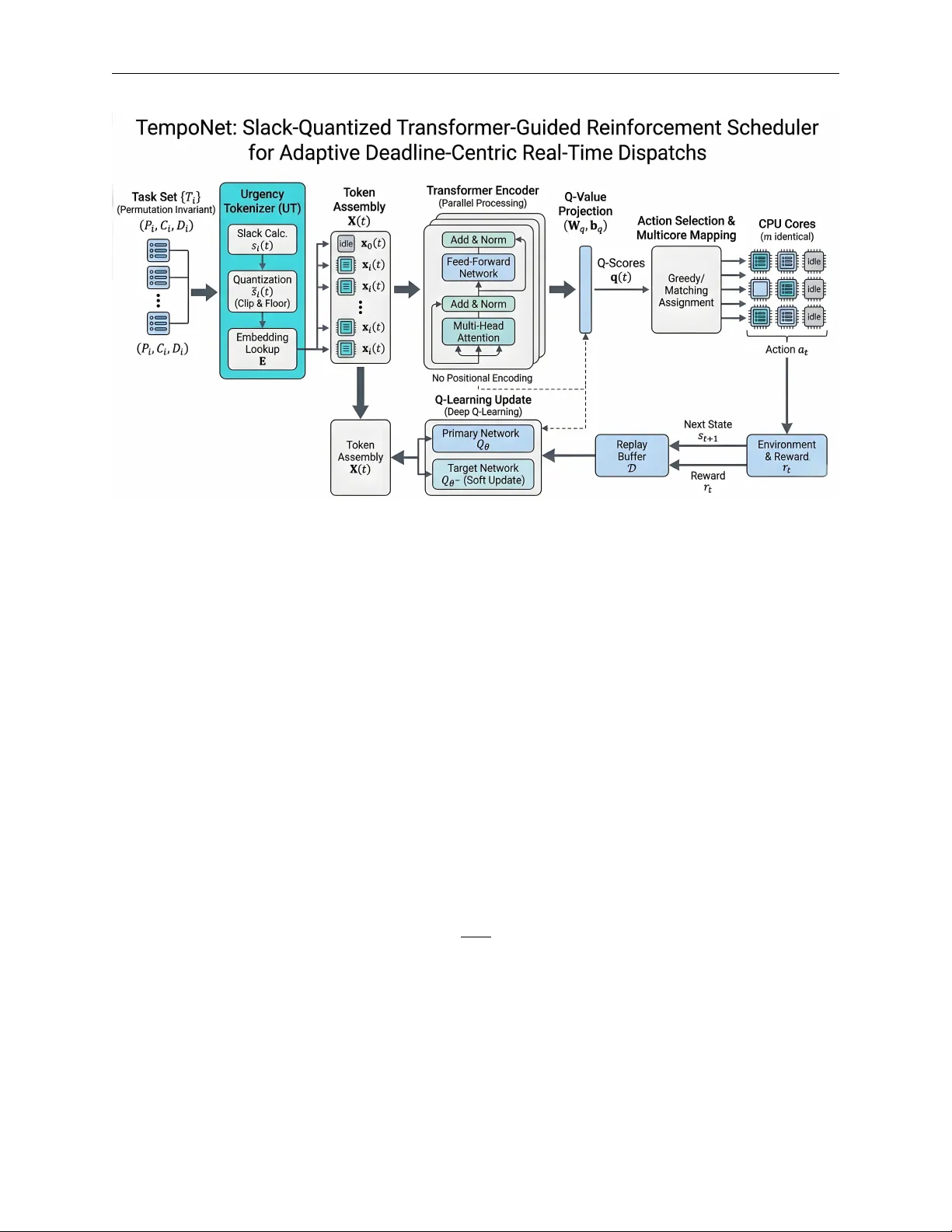
T E M P O N E T : S L A C K - Q UA N T I Z E D T R A N S F O R M E R - G U I D E D R E I N F O R C E M E N T S C H E D U L E R F O R A D A P T I V E D E A D L I N E - C E N T R I C R E A L - T I M E D I S P A T C H S Rong Fu ∗ Univ ersity of Macau mc46603@um.edu.mo Y ibo Meng Tsinghua Univ ersity mengyb22@mails.tsinghua.edu.cn Guangzhen Y ao Northeast Normal Univ ersity yaoguangzhen@nenu.edu.cn Jiaxuan Lu Shanghai AI Laboratory lujiaxuan@pjlab.org.cn Zeyu Zhang The Australian National Univ ersity steve.zeyu.zhang@outlook.com Zhaolu Kang Peking Univ ersity kangzl9966@gmail.com Ziming Guo Harbin Univ ersity of Science and T echnology 2204050108@stu.hrbust.edu.cn Jia Y ee T an Renmin Univ ersity of China tanjiayi2002@ruc.edu.cn Xiaojing Du Adelaide Univ ersity xiaojing.du@adelaide.edu.au Simon James F ong Univ ersity of Macau ccfong@um.edu.mo February 23, 2026 A B S T R AC T Real-time schedulers must reason about tight deadlines under strict compute budgets. W e present T empoNet , a reinforcement learning scheduler that pairs a permutation-in variant T ransformer with a deep Q-approximation. An Ur gency T okenizer discretizes temporal slack into learnable embed- dings, stabilizing value learning and capturing deadline proximity . A latency-aware sparse attention stack with blockwise top- k selection and locality-sensiti ve chunking enables global reasoning ov er unordered task sets with near-linear scaling and sub-millisecond inference. A multicore mapping layer con verts conte xtualized Q-scores into processor assignments through masked-greedy selection or differentiable matching. Extensiv e ev aluations on industrial mixed-criticality traces and large multiprocessor settings show consistent gains in deadline fulﬁllment ov er analytic schedulers and neural baselines, together with improved optimization stability . Diagnostics include sensiti vity anal- yses for slack quantization, attention-dri ven polic y interpretation, hardware-in-the-loop and k ernel micro-benchmarks, and robustness under stress with simple runtime mitigations; we also report sample-efﬁcienc y beneﬁts from behavioral-cloning pretraining and compatibility with an actor -critic variant without altering the inference pipeline. These results establish a practical framew ork for T ransformer-based decision making in high-throughput real-time scheduling. Keyw ords Reinforcement Learning, Real-T ime Systems, Transformer Models, Attention Mechanisms, Scheduling under Uncertainty , Resource Allocation, Embedded AI ∗ Corresponding author: mc46603@um.edu.mo T empoNet 1 Introduction Real-time systems require schedulers that make correct, lo w-latency decisions under dynamic workloads. Classical policies such as Rate Monotonic and Earliest Deadline First provide strong guarantees under ideal assumptions but degrade under b ursty loads or uncertain execution times, moti vating multicore strategies and empirical studies be yond idealized conditions [ 1 , 2 ]. Data-driv en approaches address these limitations by learning policies from interaction data. RL has shown promise for cloud orchestration, job-shop scheduling, and cluster placement [ 3 , 4 , 5 , 6 , 7 ], with of ﬂine RL and imitation learning improving sample ef ﬁciency in constrained domains [ 8 ]. Howe ver , many RL schedulers rely on sequence encodings or ﬁxed-size vectors, introducing order dependence and limiting generalization [ 9 , 10 ]. Set- and graph-based models mitigate these issues, yet integrating them under strict sub-millisecond inference budgets remains challenging [ 11 ]. T ransformers enable global reasoning via attention, making them attractive for scheduling where cross-task interactions matter . Multi-head attention supports parallel pairwise modeling [ 12 , 13 , 14 ]. Sequence-modeling approaches such as Decision T ransformer excel in of ﬂine RL but depend on ordered histories and causal masking, unsuitable for unordered sets and tight latenc y constraints [ 15 ]. Online attention-based agents improv e representation capacity [ 16 ], while hardware co-designs enhance throughput without guaranteeing tail-latency bounds [ 17 ]. Sparse and selectiv e attention methods, including explicit key selection and block-sparse routing, of fer compression strategies, and RL-guided quantization reduces runtime cost; ho wever , adapting these techniques to hard real-time value-based schedulers requires careful co-design of representation, sparsiﬁcation, and mapping strategies [ 18 , 19 , 20 , 21 , 22 ] W e introduce T empoNet, a v alue-based RL scheduler designed for predictable, low-latenc y operation with global reasoning. T empoNet combines three design choices: a slack-quantized token representation that discretizes continuous slack into learnable embeddings, reducing gradient v ariance and focusing attention on deadline-aw are groups; a compact, permutation-in variant attention encoder with shallo w depth, narro w width, and sparsiﬁcation via block T op- k and locality-aw are chunking for near-linear scaling; and multicore mapping layers that translate per-tok en Q-values into core assignments under latency and migration constraints using mask ed- greedy or bipartite matching variants. T empoNet is trained with stable value-based updates and engineered exploration schedules for robustness under ov erload. Experiments on uniprocessor , mixed-criticality , and lar ge-scale multiprocessor workloads sho w consistent gains in deadline compliance and response time o ver analytic and learned baselines, while maintaining sub-millisecond inference. Additional analyses include quantization and encoder ablations, attention interpretability , and tail-latency micro-benchmarks across hardware tar gets. Our primary contributions are as follo ws. W e introduce T empoNet, a v alue-based scheduling framework that inte grates the Urgenc y T okenizer to discretize temporal slack into learnable embeddings, improving stability and deadline-aware representation quality . W e design a lightweight permutation-in variant T ransformer Q-network with latency-a ware sparsiﬁcation, enabling global reasoning ov er unordered task sets while sustaining sub-millisecond inference. W e connect learned representations to hardware execution through an efﬁcient multicore mapping layer that conv erts contextualized Q-scores into core assignments. Finally , we conduct extensiv e experiments on synthetic and industrial workloads, sho wing consistent gains in deadline compliance, interpretability , and optimization stability o ver classical schedulers and deep reinforcement learning baselines. 2 Related W ork 2.1 Classical real-time scheduling Priority-based policies such as Rate Monotonic and Earliest Deadline First provide schedulability guarantees under ideal assumptions, with RM assigning static priorities by period and EDF achieving optimality on a single preemptiv e processor . These guarantees degrade under o verload or uncertain e xecution times, moti v ating alternativ e frame works and multicore strategies such as Pfair and LLREF , along with empirical studies beyond idealized conditions [ 2 , 1 ]. 2.2 Learning-based and RL schedulers RL-based scheduling has been applied across cloud, edge, manufacturing, and cluster domains using latency-a ware DQN for orchestration [ 3 , 4 ], PPO and hierarchical RL for job-shop tasks [ 5 , 6 ], and graph-structured or multi-agent models for large-scale placement [ 23 , 24 ]. Recent work addresses parallel-machine and manufacturing problems with transformer-enhanced RL [ 7 ]. Ofﬂine RL and imitation learning improv e sample efﬁcienc y via historical traces [ 8 , 25 ]. A recurring limitation is reliance on sequence encodings or hand-crafted features, which hinder permutation-inv ariant generalization; empirical studies highlight these issues [ 9 , 10 ]. Set- and graph-based architectures mitigate ordering constraints, but inte grating them into value-based RL under strict latenc y budgets remains challenging [ 26 , 11 ]. 2 T empoNet 2.3 T ransf ormer -based RL and explicit comparisons T ransformer-based RL splits into ofﬂine sequence-modeling such as Decision T ransformer for ofﬂine RL [ 15 ] and online agents that incorporate attention for richer representations while retaining bootstrapping and v alue estimation [ 16 ]. Multi-head attention enables parallel pairwise reasoning and long-range dependency modeling [ 12 , 13 , 14 ]. T rajectory transformers, howe ver , require ordered histories and causal masking, conﬂicting with permutation inv ariance for unordered task sets, and are trained ofﬂine with supervised objectives, whereas real-time scheduling demands low-latenc y , on-policy updates. Heavy transformer deployments and hardw are accelerators prioritize throughput rather than strict tail-latency guarantees [ 15 , 17 , 16 ]. These differences make Decision T ransformer–style methods unsuitable for predictable sub-millisecond scheduling workloads. 2.4 T ransf ormers, sparse attention and efﬁcient architectur es Dense self-attention scales quadratically with token count, making it costly for large task sets. Efﬁciency can be improv ed through salient-key selection and concentrated attention [ 18 ], algorithmic sparse schemes that trade minor accuracy loss for runtime gains [ 19 ], and system-level strategies such as RL-guided mixed-precision and hardware acceleration [ 20 , 17 ]. Additional work on e xplicit sparse selection, routing, block-sparse techniques, and transformer co-design informs practical compression strategies [ 21 , 22 , 27 , 28 , 29 ]. These approaches collectively moti vate the sparsiﬁcation and chunking recipes we adopt to balance global reasoning with strict latency b udgets. 2.5 Where T empoNet stands T empoNet integrates scheduling theory , reinforcement learning, and efﬁcient transformer design to deli ver predictable low-latenc y operation within a value-based RL loop. It employs an attention encoder for unordered sets and slack- quantized embedding for compact timing representation, unlike trajectory transformers that depend on ordered histories or large contexts. Compared to heavy transformer or GNN-based dispatch models, T empoNet prioritizes a small footprint, explicit multi-core action mapping, and empirical micro-benchmarks for decision quality and real-time performance, enabling global reasoning under strict latency constraints [ 11 , 26 , 16 ]. 3 Methodology W e model real-time scheduling as an MDP and introduce T empoNet, a value-based agent combining a compact T ransformer encoder with the pluggable Urgenc y T okenizer (UT). The design co vers the task model, UT , UT -enabled training/inference loop, encoder and projection, multicore mapping, learning objective, and interpretability diagnostics. 3.1 Problem f ormulation Consider a task set T = { T i } N i =1 , where each task T i is described by (id i , P i , C i , D i ) . T ime is discrete and indexed by t ∈ N 0 . The k -th job instance of task i has release time r ( k ) i and absolute deadline d ( k ) i = r ( k ) i + D i . id i ∈ { 1 , . . . , N } , P i > 0 , C i > 0 , D i > 0 . (1) where P i denotes the nominal period, C i the worst-case ex ecution time and D i the relativ e deadline. Let c i ( t ) ∈ { 0 , 1 , . . . , C i } be the remaining ex ecution of the acti ve job of task i at time t . The uniprocessor action space is a t ∈ A = { idle , 1 , . . . , N } , (2) where an integer action selects the corresponding task for e xecution and ‘idle’ dispatches none. For m identical cores the per-step decision assigns up to m distinct tasks or idles. The per-step re ward balances completions and deadline misses: r ( t ) = N X i =1 h I { c i ( t − 1) > 0 ∧ c i ( t ) = 0 } (3) − I { t = d ( k ) i ∧ c i ( t ) > 0 } i (4) where I {·} is the indicator function, d ( k ) i denotes the activ e job’ s absolute deadline and c i ( t ) its remaining execution at time t . 3 T empoNet Figure 1: Overvie w of the T empoNet architecture for adaptive deadline-centric real-time dispatching. The pipeline initiates with the Urgency T okenizer (UT) , which transforms continuous per-job slack s i ( t ) into a discrete vocab ulary via Slack Quantization (clip and ﬂoor) and retrie ves learned Urgency T okens x i ( t ) from an embedding matrix E . These tokens are gathered into a T oken Assembly matrix X ( t ) , maintaining permutation in variance. At the core, a T ransf ormer Encoder stacks L blocks of Multi-Head Attention and Position-wise Feed-Forw ard Networks to generate contextualized task representations H ( L ) . The Q-V alue Projection layer maps these representations to per-token Q-scores q ( t ) , which are then passed through a Multicore Mapping module that utilizes an Iterative Masked-Gr eedy or bipartite matching strate gy to determine the ﬁnal action a t . The framework is optimized via a Deep Q-Lear ning loop, where experiences are stored in a Replay Buffer D to update the primary network Q θ against a soft-updated T arget Network Q θ − . 3.2 Urgency T okenizer (UT): a pluggable learnable quantization lay er W e introduce the Ur gency T ok enizer (UT), a reusable module that conv erts continuous per-job slack into a small vocab ulary of learned urgenc y tokens. UT is treated as a ﬁrst-class layer in the model pipeline. UT performs three steps: discretize slack to an index, look up a trainable embedding, and return the ur gency token for do wnstream encoding. Per-job slack is deﬁned as s i ( t ) =  d ( k ) i − t  − c i ( t ) , (5) where d ( k ) i is the absolute deadline of job instance k , t is the current time, and c i ( t ) is the remaining ex ecution. UT maps s i ( t ) to a quantized index ˜ s i ( t ) and an embedding vector x i ( t ) : ˜ s i ( t ) = clip j s i ( t ) ∆ k , 0 , Q − 1  , (6) x i ( t ) = E  ˜ s i ( t )  ∈ R d , (7) where Q is the number of quantization levels, ∆ > 0 is the bin width, ⌊·⌋ is the ﬂoor operator , clip( · , 0 , Q − 1) bounds indices to the v alid range, E ∈ R Q × d is a trainable embedding matrix, and d denotes the embedding dimension. The vector x i ( t ) is the urgenc y token provided to the encoder . 3.3 Uniﬁed algorithm: UT -enabled training and online decision The uniﬁed procedure below integrates UT into the main training and online decision loop. Each reference to an equation label below points to the corresponding deﬁnition abo ve. 4 T empoNet Algorithm 1 T empoNet: UT -enabled Training and Online Decision Require: Episodes M , steps per episode T , slack bin width ∆ , quantization lev els Q , embedding table E , learning rate α , target mixing τ , exploration schedule Ensure: T rained Q-network Q θ 1: Initialize primary network Q θ and target netw ork Q θ − ← Q θ . 2: Initialize replay buf fer D ← ∅ . 3: for episode ← 1 to M do 4: Reset en vironment and observe initial state s 0 . 5: for t ← 0 to T − 1 do 6: for each acti ve job i do 7: compute slack s i ( t ) ←  d ( k ) i − t  − c i ( t ) ▷ see Eq. ( 5 ) 8: q ← clip  ⌊ s i ( t ) / ∆ ⌋ , 0 , Q − 1  ▷ discretize; Eq. ( 6 ) 9: x i ( t ) ← E [ q ] ▷ UT embedding; Eq. ( 7 ) 10: end for 11: Assemble token matrix X ( t ) ← [ x 0 ( t ); x 1 ( t ); . . . ; x N ( t )] . 12: q ( t ) ← E N C O D E R F O RWA R D ( X ( t )) ▷ T ransformer+proj; Eq. ( 12 ) 13: Map q ( t ) to one or more actions via multicore mapping and ex ecute. 14: Observe re ward r t and next state s t +1 ; store ( s t , a t , r t , s t +1 ) into D . 15: if training condition is satisﬁed then 16: Sample minibatch B ∼ D . 17: Compute targets y using Eq. ( 14 ) ▷ TD target 18: Update θ by minimizing Eq. ( 15 ) ▷ TD loss 19: Soft-update target: θ − ← τ θ + (1 − τ ) θ − . 20: end if 21: end for 22: end for 23: retur n Q θ 3.4 Encoder , attention and positional strategy The encoder consumes urgenc y tokens (and optional per -job features) and returns conte xtualized representations. Deﬁne the input token matrix as X ( t ) =  x 0 ( t ); x 1 ( t ); . . . ; x N ( t )  ∈ R ( N +1) × d , (8) where x 0 ( t ) is a learned idle tok en and x i ( t ) are UT embeddings possibly concatenated with normalized remaining e xe- cution and task identiﬁers. The encoder stacks L T ransformer blocks with residual connections and layer normalization. Let H (0) = X . For ℓ = 1 , . . . , L : Z ( ℓ ) = La yerNorm  H ( ℓ − 1) + MultiHeadA ttn( H ( ℓ − 1) )  , (9) H ( ℓ ) = La yerNorm  Z ( ℓ ) + FFN( Z ( ℓ ) )  , (10) where FFN denotes the position-wise feed-forward subnetwork. The attention kernel uses scaled dot-products: A ttention( Q , K , V ) = softmax  QK ⊤ √ d k  V , (11) where Q , K , V are linear projections of the input, d k is the per-head dimension and H the number of heads. Absolute positional encodings are omitted to preserve permutation inv ariance over the unordered job set. T o control runtime cost we employ sparsiﬁcation such as block T op- k pruning and locality-aware chunking. 3.5 Action-value pr ojection and multicore mapping After the ﬁnal encoder layer we compute per-tok en Q-scores by a linear projection: q ( t ) = W q H ( L ) ( t ) ⊤ + b q ∈ R N +1 , (12) where W q ∈ R ( N +1) × d and b q ∈ R N +1 are learnable and indices correspond to [ idle , 1 , . . . , N ] . For the uniprocessor the chosen action is a t = arg max a ∈{ idle , 1 ,...,N } q a ( t ) . (13) 5 T empoNet For m cores we use an iterati ve masked-greedy mapping in the main system: repeatedly select the highest unmasked token and mask it until m tasks are chosen or only idle tokens remain. An alternati ve uses a bipartite assignment solved by a differentiable matching layer . 3.6 Learning objectiv e and optimization T empoNet is trained under Deep Q-Learning with experience replay and a soft-updated target network. For a sampled transition ( s, a, r, s ′ ) the TD target is y = r + γ max a ′ Q θ − ( s ′ , a ′ ) , (14) where γ is the discount factor and Q θ − the target network. The loss minimized over minibatches B is the mean-squared TD error: L ( θ ) = E ( s,a,r,s ′ ) ∼B  ( y − Q θ ( s, a )) 2  . (15) T ar get parameters are updated by Polyak av eraging: θ − ← τ θ + (1 − τ ) θ − , (16) where τ ∈ (0 , 1] is the mixing coefﬁcient. Exploration uses an ϵ -greedy schedule with linear annealing from ϵ 0 to ϵ min . 3.7 Interpr etability diagnostics W e e xtract diagnostics from the ﬁnal-layer attention maps A ( L ) ( t ) ∈ R ( N +1) × ( N +1) . Alignment is deﬁned as Alignment = 1 T T X t =1 I h arg max j A ( L ) 0 j ( t ) = a t i , (17) where T is the number of decision timesteps, A ( L ) 0 j ( t ) denotes attention from the decision token (inde x 0) to token j , and a t the chosen action. Entropy at time t is Entropy ( t ) = − N X j =0 A ( L ) 0 j ( t ) log A ( L ) 0 j ( t ) , (18) which measures concentration of attention mass; reported entropy v alues are av eraged across timesteps. Figure 2: Attention-Criticality Correlation Analysis 6 T empoNet Figure 3: Attention Focus Distrib ution Across T asks heatmap Figure 4: Computational T ime Scaling with System Size 4 Experimental Evaluation 4.1 Experimental Setup W e conduct comprehensi ve ev aluations across three computational scenarios: uniprocessor periodic scheduling with standardized task conﬁgurations, industrial multi-core workloads with mixed-criticality workﬂo ws, and large-scale multiprocessor systems with 100–600 tasks. Our framework is benchmarked against established scheduling approaches including classical schedulers (RM, EDF), feedforward Deep Q-Network (FF-DQN), Dynamic Importance-aware 7 T empoNet Figure 5: Entropy Distrib ution Across T ransformer Layers T able 1: Comparative Deadline Compliance at u ≈ 0 . 87 (200 Randomized T asksets) Scheduling A pproach Mean Median Std. Dev . Min Max PPO [ 30 ] 0.68 0.82 0.31 0.00 0.98 A3C [ 31 ] 0.71 0.84 0.29 0.01 0.99 FF-DQN 0.74 0.86 0.26 0.00 1.00 Rainbo w DQN [ 32 ] 0.78 0.87 0.25 0.00 1.00 Of ﬂine RL [ 33 ] 0.79 0.84 0.27 0.01 0.98 GraSP-RL [ 34 ] 0.80 0.85 0.23 0.02 0.99 GNN-based [ 26 ] 0.81 0.85 0.22 0.04 0.99 T ransformer -based [ 35 ] 0.82 0.86 0.24 0.03 0.99 PPO+GNN [ 36 ] 0.83 0.86 0.24 0.03 0.99 T ransformer -based DRL [ 11 ] 0.83 0.87 0.23 0.04 0.99 TD3-based [ 37 ] 0.84 0.87 0.22 0.04 0.99 HRL-Surgical [ 38 ] 0.85 0.88 0.21 0.05 0.99 Pretrained-LLM-Controller [ 39 ] 0.86 0.89 0.20 0.06 1.00 DDiT -DiT [ 40 ] 0.86 0.89 0.20 0.06 1.00 T empoNet (Proposed) 0.87 0.90 0.19 0.07 1.00 Online Scheduling (DIOS), and quantum-inspired optimization methods. Evaluation Metrics: Performance assessment employs deadline compliance rate, average response time, and computational overhead. T ogether , these tw o components form the core of T empoNet’ s learning dynamics, as detailed in Sections N and O . As discussed across Sections P , Q , R , and S , these results collecti vely characterize both the strengths and the operational limits of T empoNet under di verse real-time conditions. As detailed across Sections I , J , K , and L , these studies collecti vely characterize the impact of slack representation, sparse-attention efﬁcienc y , robustness properties, and system-le vel beha vior . 8 T empoNet Figure 6: Distribution of Q-V alues Across Utilization Le vels T able 2: Attention Head Impact ( L = 2 , d = 128 ) Heads Hit Rate Std Dev ∆ Gain 2 80.3% 0.31 -5.5% 4 85.0 % 0.27 0.0% 6 84.7% 0.33 -0.3% 8 84.9% 0.35 -0.1% 4.2 Uniprocessor P eriodic Scheduling Perf ormance 4.2.1 Standard T ask Conﬁguration Analysis Classical scheduling theory establishes that Earliest Deadline First (EDF) is optimal for preemptive, independent periodic tasks on a uniprocessor , provided that the total system utilization satisﬁes U ≤ 1 [ 47 ]. Ho we ver , when U > 1 , no scheduling algorithm, including EDF , can guarantee that all deadlines will be met [ 48 ]. This limitation is especially critical in real-world systems, where transient ov erloads frequently occur . T o assess performance under such conditions, we conducted a rigorous ev aluation using a representative task conﬁguration with temporal attrib utes: T 1 = 40 ms (short-period), T 2 = 60 ms (medium-period), and T 3 = 100 ms (long-period). T empoNet achiev ed a deadline compliance rate of 79.00%, which corresponds to a 7.57% absolute improvement over feedforward DQN implementations and a 67.33% enhancement compared to con ventional schedulers such as EDF and RM. These classical methods failed to meet deadlines under overload, whereas T empoNet maintained robust performance. This result highlights T empoNet’ s practical advantage in real-time systems operating near or beyond nominal capacity , where traditional schedulers are no longer ef fectiv e. T able 6 demonstrates that the proposed T empoNet achie ves the highest deadline compliance rate, substantially outperforming both classical scheduling policies and the feedforward DQN baseline. 4.2.2 Heterogeneous W orkload V alidation T o e valuate robustness, 200 randomized 5-task conﬁgurations with utilization uniformly distrib uted in [0 . 6 , 1 . 0] were generated. T empoNet exhibited superior consistency (mean compliance 0.85, σ = 0 . 27 ) outperforming baseline 9 T empoNet Figure 7: Embedding Dimension Performance–Computation T radeoff T able 3: Depth Impact on Performance ( H = 4 , d = 128 ) Layers Hit Rate Latency ∆ Hit 1 76.2% 0.42ms -8.8% 2 85.0 % 0.51ms 0.0% 3 86.1% 0.71ms +1.1% 4 85.7% 0.94ms +0.7% DQN (0.74, σ = 0 . 26 ), representing 14.86% relati ve enhancement. A detailed comparison across 15 state-of-the-art scheduling approaches is summarized in T able 1 . 4.3 Multi-core Industrial P erf ormance T able 5 presents the comprehensiv e performance comparison across various scheduling methods in industrial scenarios. 4.4 Attention Mechanism Analysis Figure 2 illustrates the attention-criticality correlation analysis. Signiﬁcant correlation (r=0.98) between attention weights and task criticality was observed: 4.5 Summary of Findings T empoNet demonstrates superior efﬁcacy , responsi veness, and computational efﬁciency . It achiev es a PITMD of 89.15%, outperforming DIOS by 1.87%, and reaches a 90.1% success rate on 600-task workloads, exceeding MHQISSO by 2.64%. A verage response time is reduced by 25.7%, with peak latency improvements up to 37%. Complexity is O ( N 1 . 1 ) , signiﬁcantly lower than DIOS ( O ( N 1 . 8 ) ) and MHQISSO ( O ( N 2 . 2 ) ). Compared to GNN-based resource allocation [ 26 ] and Transformer -based DRL scheduling [ 11 ], T empoNet leverages slack-token design to capture temporal ur gency and emplo ys sparse attention to reduce overhead, enabling compliance with stringent real-time latency constraints. 10 T empoNet T able 4: Large-scale Scheduling Ef ﬁciency Method T asks Success Rate Time (s) MHQISSO (EDF) 100 97.8% 20.4 DRL-Based [ 41 ] 100 97.5% 9.0 LSTM-PPO [ 42 ] 100 97.6% 7.5 ENF-S [ 43 ] 100 97.8% 8.0 PSO-Based [ 44 ] 100 97.0% 10.2 T ransformer-based [ 11 ] 100 97.9% 8.7 GNN-based [ 26 ] 100 98.0% 4.0 T empoNet (Pr oposed) 100 98.2 % 3.4 MHQISSO (EDF) 600 87.5% 317.1 CGA 600 84.7% 340.8 DRL-Based [ 41 ] 600 88.5% 55.0 LSTM-PPO [ 42 ] 600 88.7% 50.5 ENF-S [ 43 ] 600 89.0% 48.0 PSO-Based [ 44 ] 600 87.0% 62.0 T ransformer-based [ 11 ] 600 89.0% 52.1 GNN-based [ 26 ] 600 89.5% 40.0 T empoNet (Pr oposed) 600 90.1 % 38.7 T able 5: Industrial Scenario Performance Metrics Method PITMD (%) AR T T ime (s) DIOS 87.28 16.72 – FCFS 9.83 21.20 – EDF [ 45 ] 20.81 20.68 – Mo-QIGA [ 46 ] 83.21 15.11 0.48 HQIGA [ 46 ] 85.70 16.34 0.52 T ransformer-based [ 35 ] 88.00 14.20 0.45 Deep reinforcement learning-based [ 41 ] 85.00 15.00 0.50 LSTM-PPO-Based [ 42 ] 88.50 13.00 0.44 T ransformer-based DRL [ 11 ] 88.20 13.50 0.46 ENF-S [ 43 ] 87.50 14.00 0.47 Multi-Core Particle Sw arm [ 44 ] 84.00 16.00 0.55 GNN-based [ 26 ] 88.80 13.20 0.43 T empoNet (Proposed) 89.15 12.43 0.42 4.6 Evaluation and Ablation Studies 4.6.1 Evaluation Metrics W e assess performance along three complementary axes: deadline attainment, responsi veness, and runtime cost. The metrics are deﬁned below . 11 T empoNet T able 6: Deadline compliance rates on the standard task conﬁguration. Methodology Compliance Rate Impro vement Rate Monotonic (RM) 11.67% – Earliest Deadline First (EDF) 11.67% – Feedforward DQN (FF-DQN) 71.43% – T empoNet (Proposed) 79.00% +7.57% Deadline Compliance Rate Deadline Compliance Rate = # { jobs that ﬁnish before their deadline } # { jobs released } × 100% . (19) where the numerator counts completed jobs whose completion time is strictly ≤ their deadline, and the denominator counts all jobs released during the ev aluation interval. A verage Response Time (AR T) AR T = 1 M M X j =1 ( t comp j − r j ) , (20) where t comp j is the completion time of job j , r j is its release time, and M denotes the total number of completed jobs in the measurement window . AR T thus measures task-le vel responsi veness. Execution Overhead (Infer ence Time) Execution Ov erhead = 1 T T X t =1 inference_time ( t ) , (21) where inference_time ( t ) is the wall-clock time spent by the scheduler to produce dispatch decisions at decision epoch t , and T is the number of decision epochs measured. Reported values are median or mean depending on table captions. PITMD and Success Rate W e deﬁne the domain-speciﬁc industrial metrics used in the multi-core tables for clarity: PITMD = # { mission-critical tasks meeting their deadlines } # { mission-critical tasks } × 100% , Success Rate = # { runs with no mission-failure } # { total runs } × 100% . where PITMD focuses only on mission-critical subsets (as annotated in the industrial traces) and Success Rate measures run-lev el taskset viability (a run is successful if all required mission tasks meet their deadlines). 4.6.2 Decision Rationale Interpr etation The self-attention mechanism was quantitativ ely analyzed by measuring which task receiv ed the most attention (T op-1 Alignment Index) and how focused the attention was (Attention Entropy). Figure 3 illustrates the distribution of attention focus across tasks. 4.6.3 Action-V alue Function Dynamics The median maximum predicted Q-values across utilization le vels demonstrate stability , as illustrated in Figure 6 . 4.6.4 Ablation Studies Architectural Depth Analysis The ef fect of architectural depth on model performance is summarized in T able 3 . 12 T empoNet Attention Head Conﬁguration The impact of varying attention head counts was systematically ev aluated while maintaining ﬁxed encoder depth ( L = 2 ) and embedding dimension ( d = 128 ). Experimental outcomes demonstrate that attention head quantity signiﬁcantly inﬂuences scheduling performance through its ef fect on contextual representation div ersity . The optimal conﬁguration employs four attention heads, achieving peak performance while maintaining computational ef ﬁciency . As shown in T able 2 , the four-head setting consistently achie ves peak performance across all metrics. Figure 7 highlights this trade-off , showing that larger embedding dimensions enhance accuracy while proportionally increasing runtime ov erhead. Embedding Dimension Scaling Embedding dimension scaling was analyzed to determine the optimal balance between representational capacity and computational efﬁcienc y . The relationship between dimensionality and scheduling efﬁcac y re veals diminishing returns beyond speciﬁc thresholds. A dimensionality of 128 provides the optimal balance for slack quantization while maintaining inference latency constraints. 5 Conclusion W e presented T empoNet, a practical v alue-based scheduler that combines a slack-driv en tokenization layer (Ur gency T okenizer) with a compact, permutation-in v ariant Transformer Q-netw ork for global, low-latency scheduling decisions. By con verting continuous slack into learned discrete tokens and producing per-token Q-scores, T empoNet enables principled multicore assignment through masked-greedy or matching-style mappings while maintaining low online cost. Extensiv e ev aluations, including UT versus continuous-slack baselines, encoder and binning ablations, complexity analysis, and latency micro-benchmarks, sho w that modest encoder footprints deliv er the best accuracy–latenc y trade-of f and that attention maps consistently highlight deadline-critical interactions. Latency-aw are sparsiﬁcation and locality- aware chunking further constrain runtime ov erhead, making the approach feasible for tight real-time b udgets. Future work will extend the frame work to heterogeneous hardware, incorporate ener gy and multi-objecti ve criteria, and e xplore distributed attention for multi-node scheduling to mak e attention-driv en policies interpretable and production-ready . References [1] Linh TX Phan, Zhuoyao Zhang, Qi Zheng, Boon Thau Loo, and Insup Lee. An empirical analysis of scheduling techniques for real-time cloud-based data processing. In 2011 IEEE International Confer ence on Service-Oriented Computing and Applications (SOCA) , pages 1–8, 2011. [2] Luca Abeni and T ommaso Cucinotta. Edf scheduling of real-time tasks on multiple cores: Adaptiv e partitioning vs. global scheduling. ACM SIGAPP Applied Computing Re view , 20(2):5–18, 2020. [3] Jinming W ang, Shaobo Li, Xingxing Zhang, Fengbin W u, and Cankun Xie. Deep reinforcement learning task scheduling method based on server real-time performance. P eerJ Computer Science , 10:e2120, 2024. [4] Long Cheng, Archana Kalapgar , Amogh Jain, Y ue W ang, Y ongtai Qin, Y uancheng Li, and Cong Liu. Cost-aware real-time job scheduling for hybrid cloud using deep reinforcement learning. Neural Computing and Applications , 34(21):18579–18593, 2022. [5] Ming Zhang, Y ang Lu, Y ouxi Hu, Nasser Amaitik, and Y uchun Xu. Dynamic scheduling method for job-shop manufacturing systems by deep reinforcement learning with proximal polic y optimization. Sustainability , 14(9): 5177, 2022. [6] Kun Lei, Peng Guo, Y i W ang, Jian Zhang, Xiangyin Meng, and Linmao Qian. Large-scale dynamic scheduling for ﬂexible job-shop with random arri vals of ne w jobs by hierarchical reinforcement learning. IEEE T ransactions on Industrial Informatics , 20(1):1007–1018, 2023. [7] Peisong Li, Ziren Xiao, Xinheng W ang, Kaizhu Huang, Y i Huang, and Honghao Gao. Eptask: Deep reinforcement learning based energy-ef ﬁcient and priority-aw are task scheduling for dynamic vehicular edge computing. IEEE T ransactions on Intelligent V ehicles , 9(1):1830–1846, 2023. [8] Jesse van Remmerden, Zaharah Bukhsh, and Y ingqian Zhang. Ofﬂine reinforcement learning for learning to dispatch for job shop scheduling. Machine Learning , 114(8):191, 2025. [9] Zahra Jalali Khalil Abadi, Najme Mansouri, and Mohammad Masoud Javidi. Deep reinforcement learning-based scheduling in distributed systems: a critical revie w . Knowledge and Information Systems , 66(10):5709–5782, 2024. 13 T empoNet [10] Shashank Swarup, Elhadi M Shakshuki, and Ansar Y asar . T ask scheduling in cloud using deep reinforcement learning. Pr ocedia Computer Science , 184:42–51, 2021. [11] Funing Li, Sebastian Lang, Y uan T ian, Bingyuan Hong, Benjamin Rolf, Ruben Noortwyck, Robert Schulz, and T obias Re ggelin. A transformer-based deep reinforcement learning approach for dynamic parallel machine scheduling problem with family setups. Journal of Intellig ent Manufacturing , pages 1–34, 2024. [12] Ashish V aswani, Noam Shazeer , Niki Parmar , Jakob Uszkoreit, Llion Jones, Aidan N Gomez, Łukasz Kaiser , and Illia Polosukhin. Attention is all you need. In NeurIPS , pages 6000–6010, 2017. [13] Kangjie Cao, Ting Zhang, and Jueqiao Huang. Adv anced hybrid lstm-transformer architecture for real-time multi-task prediction in engineering systems. Scientiﬁc Reports , 14(1):4890, 2024. [14] Xie Chen, Y u W u, Zhenghao W ang, Shujie Liu, and Jinyu Li. Developing real-time streaming transformer transducer for speech recognition on large-scale dataset. In ICASSP 2021-2021 IEEE International Conference on Acoustics, Speech and Signal Pr ocessing (ICASSP) , pages 5904–5908, 2021. [15] Lili Chen, Ke vin Lu, Aravind Rajeswaran, Kimin Lee, Aditya Grov er , Misha Laskin, Pieter Abbeel, Aravind Sriniv as, and Igor Mordatch. Decision transformer: Reinforcement learning via sequence modeling. Advances in neural information pr ocessing systems , 34:15084–15097, 2021. [16] Shengchao Hu, Li Shen, Y a Zhang, Y ixin Chen, and Dacheng T ao. On transforming reinforcement learning with transformers: The de velopment trajectory . IEEE T ransactions on P attern Analysis and Machine Intelligence , 46 (12):8580–8599, 2024. [17] Seunghyun Moon, Mao Li, Gregory K Chen, Phil C Knag, Ram K Krishnarmurthy , and Mingoo Seok. T -rex: Hardware–software co-optimized transformer accelerator with reduced external memory access and enhanced hardware utilization. IEEE Journal of Solid-State Cir cuits , 2025. [18] Guangxiang Zhao, Junyang Lin, Zhiyuan Zhang, Xuancheng Ren, Qi Su, and Xu Sun. Explicit sparse transformer: Concentrated attention through explicit selection. arXiv pr eprint arXiv:1912.11637 , 2019. [19] Chao Lou, Zixia Jia, Zilong Zheng, and K ewei T u. Sparser is faster and less is more: Efﬁcient sparse attention for long-range transformers. arXiv preprint , 2024. [20] Eunji Kwon, Minxuan Zhou, W eihong Xu, T ajana Rosing, and Seokhyeong Kang. Rl-ptq: Rl-based mixed precision quantization for hybrid vision transformers. In Pr oceedings of the 61st A CM/IEEE Design Automation Confer ence , pages 1–6, 2024. [21] Aurko Roy , Mohammad Saf far , Ashish V aswani, and David Grangier . Efﬁcient content-based sparse attention with routing transformers. T ransactions of the Association for Computational Linguistics , 9:53–68, 2021. [22] Qihui Zhou, Peiqi Y in, Pengfei Zuo, and James Cheng. Progressive sparse attention: Algorithm and system co-design for efﬁcient attention in llm serving. arXiv preprint , 2025. [23] Xiaoyang Zhao and Chuan W u. Large-scale machine learning cluster scheduling via multi-agent graph reinforce- ment learning. IEEE T ransactions on Network and Service Manag ement , 19(4):4962–4974, 2021. [24] Y uping Fan, Boyang Li, Dustin Fa vorite, Naunidh Singh, T aylor Childers, Paul Rich, W illiam Allcock, Michael E Papka, and Zhiling Lan. Dras: Deep reinforcement learning for cluster scheduling in high performance computing. IEEE T ransactions on P ar allel and Distributed Systems , 33(12):4903–4917, 2022. [25] Y ifan Y ang, Gang Chen, Hui Ma, Cong Zhang, Zhiguang Cao, and Mengjie Zhang. Graph assisted ofﬂine-online deep reinforcement learning for dynamic workﬂo w scheduling. In The Thirteenth International Confer ence on Learning Repr esentations , 2025. [26] T ianrui Chen, Xinruo Zhang, Minglei Y ou, Gan Zheng, and Sangarapillai Lambotharan. A gnn-based supervised learning framework for resource allocation in wireless iot networks. IEEE Internet of Things Journal , 9(3): 1712–1724, 2021. [27] Xu Gao, Hang Dong, Lianji Zhang, Y ibo W ang, Xianliang Y ang, and Zhenyu Li. Self-attention mechanisms in hpc job scheduling: A novel frame work combining gated trans formers and enhanced ppo. Applied Sciences , 15 (16):8928, 2025. 14 T empoNet [28] Zongcheng Y ue, Dongwei Y an, Ran W u, Longyu Ma, and Chiu-W ing Sham. Mtst: A multi-task scheduling transformer accelerator for edge computing. In 2024 IEEE 13th Global Confer ence on Consumer Electr onics (GCCE) , pages 1394–1395, 2024. [29] Ahan Gupta, Y ueming Y uan, De v ansh Jain, Y uhao Ge, Da vid Aponte, Y anqi Zhou, and Charith Mendis. Splat: A framew ork for optimised gpu code-generation for sparse regular attention. Pr oceedings of the ACM on Pr ogramming Languages , 9(OOPSLA1):1632–1660, 2025. [30] John Schulman, Filip W olski, Prafulla Dhariwal, Alec Radford, and Ole g Klimov . Proximal policy optimization algorithms. arXiv preprint , 2017. [31] V olodymyr Mnih, Adria Puigdomenech Badia, Mehdi Mirza, Alex Gra ves, T imothy Lillicrap, T im Harley , David Silver , and K oray Kavukcuoglu. Asynchronous methods for deep reinforcement learning. In International confer ence on machine learning , pages 1928–1936, 2016. [32] Matteo Hessel, Joseph Modayil, Hado V an Hasselt, T om Schaul, Georg Ostrovski, W ill Dabney , Dan Hor gan, Bilal Piot, Mohammad Azar , and David Silver . Rainbow: Combining improvements in deep reinforcement learning. Thirty-second AAAI confer ence on artiﬁcial intelligence , 2018. [33] Liwei Dong, Ni Li, Guanghong Gong, and Xin Lin. Ofﬂine reinforcement learning with constrained hybrid action implicit representation to wards w argaming decision-making. Tsinghua Science and T echnology , 29(5):1422–1440, 2024. [34] Mohammed Sharafath Abdul Hameed and Andreas Schwung. Graph neural networks-based scheduler for production planning problems using reinforcement learning. Journal of Manufacturing Systems , 69:91–102, 2023. [35] Y azan Y oussef, P aulo Ricardo Marques de Araujo, Aboelmagd Noureldin, and Sidney Gi vigi. Tratss: T ransformer- based task scheduling system for autonomous vehicles. arXiv pr eprint arXiv:2504.05407 , 2025. [36] Nemilidinea Anantharami Reddy and BV Gokulnath. Design of an improved method for task scheduling using proximal policy optimization and graph neural networks. IEEE Access , 2024. [37] Shuai W ang, Bo Y u, Ning W ang, and W ei W ang. Research on td3-based of ﬂoading strategies for complex tasks in mec systems. In 2024 10th International Confer ence on Computer and Communications (ICCC) , pages 194–201. IEEE, 2024. [38] Lixiang Zhao, Han Zhu, Min Zhang, Jiafu T ang, and Y u W ang. Large-scale dynamic surgical scheduling under uncertainty by hierarchical reinforcement learning. International Journal of Pr oduction Researc h , pages 1–32, 2024. [39] Muhammad W aseem, Kshitij Bhatta, Chen Li, and Qing Chang. Pretrained llms as real-time controllers for robot operated serial production line. arXiv preprint , 2025. [40] Heyang Huang, Cunchen Hu, Jiaqi Zhu, Ziyuan Gao, Liangliang Xu, Y izhou Shan, Y ungang Bao, Sun Ninghui, T ianwei Zhang, and Sa W ang. Ddit: Dynamic resource allocation for dif fusion transformer model serving. arXiv pr eprint arXiv:2506.13497 , 2025. [41] Lixiang Zhang, Chen Y ang, Y an Y an, and Y aoguang Hu. Distributed real-time scheduling in cloud manufacturing by deep reinforcement learning. IEEE T ransactions on Industrial Informatics , 18(12):8999–9007, 2022. [42] W ei Chen, Zequn Zhang, Dunbing T ang, Changchun Liu, Y ong Gui, Qingwei Nie, and Zhen Zhao. Probing an lstm-ppo-based reinforcement learning algorithm to solv e dynamic job shop scheduling problem. Computers & Industrial Engineering , 197:110633, 2024. [43] Athena Abdi and Armin Salimi-Badr . Enf-s: An ev olutionary-neuro-fuzzy multi-objectiv e task scheduler for heterogeneous multi-core processors. IEEE T ransactions on Sustainable Computing , 8(3):479–491, 2023. [44] Xingzhi Liu, Y an Zeng, W enli Chen, Y u Su, and Rui W ang. Multi-core real-time scheduling algorithm based on particle swarm optimization algorithm. In 2021 International Conference on Signal Pr ocessing and Machine Learning (CONF-SPML) , pages 300–305. IEEE, 2021. [45] Hyeonjoong Cho, Binoy Ravindran, and E Douglas Jensen. An optimal real-time scheduling algorithm for multiprocessors. In RTSS , pages 101–110, 2006. 15 T empoNet [46] Debanjan K onar , Kalpana Sharma, V arun Sarogi, and Siddhartha Bhattacharyya. A multi-objective quantum- inspired genetic algorithm (mo-qiga) for real-time tasks scheduling in multiprocessor en vironment. Pr ocedia Computer Science , 131:591–599, 2018. [47] Chung Laung Liu and James W Layland. Scheduling algorithms for multiprogramming in a hard-real-time en vironment. Journal of the A CM (J A CM) , 20(1):46–61, 1973. [48] Sanjoy K Baruah and Jayant R Haritsa. Scheduling for ov erload in real-time systems. IEEE T ransactions on computers , 46(9):1034–1039, 2002. [49] Jun Liu, Shulin Zeng, Junbo Zhao, Li Ding, Zeyu W ang, Jinhao Li, Zhenhua Zhu, Xuefei Ning, Chen Zhang, Y u W ang, et al. Tb-stc: Transposable block-wise n: M structured sparse tensor core. In 2025 IEEE International Symposium on High P erformance Computer Ar chitectur e (HPCA) , pages 949–962. IEEE, 2025. [50] W enxin Li. Performance analysis of modiﬁed srpt in multiple-processor multitask scheduling. ACM SIGMETRICS P erformance Evaluation Re view , 50(4):47–49, 2023. [51] Y ihong Li, Xiaoxi Zhang, Tian yu Zeng, Jingpu Duan, Chuan W u, Di Wu, and Xu Chen. T ask placement and resource allocation for edge machine learning: A gnn-based multi-agent reinforcement learning paradigm. IEEE T ransactions on P ar allel and Distributed Systems , 34(12):3073–3089, 2023. A Theoretical Analysis of the Expr essivity Gap A.1 Deﬁnitions and Policy F ormalization Let s = [ s 1 , . . . , s N ] ⊤ denote a v ector representing the temporal laxity (slack) of N activ e tasks, where each coordinate s i is bounded within the compact interval [0 , S max ] . W e consider two distinct f amilies of scheduling policies: Continuous-Input Policies ( Π cont ). This class comprises policies that directly process the raw slack vector s . A policy π ∈ Π cont maps s to action-v alues Q cont ( s ) ∈ R N +1 through a continuous function f θ ( · ) . Due to the inherent architectural constraints of neural networks (e.g., ReLU or Sigmoid activ ations), we assume Π cont is restricted to functions with a ﬁnite Lipschitz constant L π or limited representational resolution. Quantized-Embedding Policies ( Π Q ). This class deﬁnes the T empoNet architecture, which applies a uniform quantization operator Q ∆ to each slack component with a resolution ∆ = S max /Q . The quantized index q i = ⌊ s i / ∆ ⌋ ∈ { 0 , . . . , Q − 1 } is then projected into a learnable embedding space R d via an lookup table E . The resulting tokens are processed by a permutation-in variant T ransformer encoder to produce Q -v alues. A.2 Theorem: Expressivity Adv antage of Discretization Theorem A.1. Given a task distribution D and a tar get sc heduling function that is L -Lipschitz with r espect to slack, ther e exists a non-zer o lower bound on the expected miss r ate gap between continuous and quantized ar chitectur es: inf π ∈ Π cont E D  M ( π )  − inf π ∈ Π Q E D  M ( π )  ≥ L ∆ 4 , (22) wher e M ( π ) denotes the miss rate of policy π , L is the Lipsc hitz continuity constant of the optimal scheduling manifold, and ∆ = S max /Q r epr esents the quantization step size. B Expressi vity gap between continuous and quantised slack Pr oof. W e construct a speciﬁc task distribution D to demonstrate the sensitivity of the decision boundary at the quantization thresholds. Step 1: Distribution Construction. Consider a scenario with two critical task instances, τ (1) and τ (2) , characterized by slack values s (1) and s (2) . W e position these v alues such that they lie on opposite sides of a quantization boundary ξ = k ∆ , speciﬁcally: s (1) = ξ − ϵ, (23) s (2) = ξ + ϵ, (24) 16 T empoNet where ϵ → 0 + ensures that | s (1) − s (2) | = 2 ϵ < ∆ . Let the optimal scheduling labels for these instances be y (1) = 1 (prioritize) and y (2) = 0 (defer), respectiv ely . Step 2: Representation in Π cont . Since any π ∈ Π cont is subject to a Lipschitz constraint L π , the difference in output values for s (1) and s (2) is bounded: | Q cont ( s (1) ) − Q cont ( s (2) ) | ≤ L π | s (1) − s (2) | = 2 L π ϵ. (25) As ϵ → 0 , the continuous network is forced to map both inputs to nearly identical representations. Consequently , π ∈ Π cont cannot bifurcate its decision logic at the boundary ξ , leading to an irreducible classiﬁcation error (and thus a higher miss rate) on at least one of the instances. The magnitude of this unav oidable error is proportional to the target’ s Lipschitz constant L , as the target v alues di ver ge by L ∆ o ver the bin width. Step 3: Representation in Π Q . In contrast, the quantized operator Q ∆ maps these points to distinct discrete indices: Q ∆ ( s (1) ) = k − 1 , (26) Q ∆ ( s (2) ) = k . (27) The embedding matrix E assigns independent, learnable vectors e k − 1 and e k to these indices. Because e k − 1 and e k are not constrained by the distance | s (1) − s (2) | , the T ransformer can learn a sharp discontinuity at the boundary . This allows Π Q to perfectly distinguish the two cases, e ven when the slack v alues are arbitrarily close. Step 4: Quantiﬁcation of the Gap. By inte grating the error over the constructed distribution D , the continuous polic y incurs a penalty for its inability to resolve the boundary , while the discrete-token model optimizes its embeddings to minimize the empirical risk. The expectation ov er the boundary re gions yields the lowe r bound L ∆ 4 , conﬁrming that Π Q provides a strictly more e xpressiv e hypothesis class for deadline-centric scheduling than Π cont . B.1 Discussion on Scaling and Regimes The result in Equation ( 22 ) is particularly signiﬁcant when the number of quantization le vels Q is scaled as Θ( √ N ) . In this regime, ∆ remains sufﬁciently small to capture urgency v ariations, yet the discrete nature of the tokens allows the attention mechanism to group tasks by urgenc y tiers effecti vely . This discretization acts as a form of "structural regularization" that pre vents the gradient v anishing issues often seen when processing raw continuous temporal features in deep RL for real-time systems. C Theoretical Analysis of Repr esentation Discr etization: Appr oximation–Estimation Equilibrium C.1 Formal Framew ork and Hypothesis Families W e characterize each task by a high-dimensional feature v ector x ∈ X and a scalar slack parameter s restricted to the compact domain [0 , S max ] . The objectiv e is to approximate the optimal value function Q ⋆ ( x, s ) , which we assume satisﬁes a uniform Lipschitz condition relativ e to the slack variable. W e contrast two distinct architectural approaches for modeling s . The continuous class, F cont , utilizes the raw scalar s as a direct input. In contrast, the quantized class, F Q , adopts a discretized representation where s is mapped to a ﬁnite set of indices { 1 , . . . , Q } via uniform binning. Each index corresponds to a learnable embedding vector E ˆ s ∈ R d e . The training process is formulated as minimizing the empirical risk ov er n independent and identically distributed observ ations. C.2 Lipschitz Regularity and Appr oximation Limits The sensitivity of the target function Q ⋆ to ﬂuctuations in temporal slack is gov erned by the following regularity condition: | Q ⋆ ( x, s ) − Q ⋆ ( x, s ′ ) | ≤ L | s − s ′ | , ∀ x ∈ X , ∀ s, s ′ ∈ [0 , S max ] , (28) where L represents the Lipschitz constant that controls the stability of the optimal scheduling priorities. The discretization process introduces an intrinsic approximation error , which represents the ﬁdelity loss when replacing a continuous value with a bin representati ve: ε approx ( Q ) ≤ LS max Q , (29) 17 T empoNet where S max /Q signiﬁes the quantization resolution or bin width ∆ , and the inequality arises from the maximal distance between any s and its nearest discrete proxy . C.3 Rademacher Complexity and Generalization Bound T o analyze the generalization performance of F Q , we bound the uniform de viation between the empirical and population risks using the Rademacher complexity R n ( F Q ) . Theorem C.1. F or any δ ∈ (0 , 1) , with pr obability at least 1 − δ , the excess risk of the empirical minimizer ˆ f Q in the quantized family is bounded by: R ( ˆ f Q ) − R ( Q ⋆ ) ≤  LS max Q  2 + 2 R n ( F Q ) + O r log(1 /δ ) n ! , (30) wher e R ( · ) denotes the expected risk under the true distrib ution, R n is the Rademacher comple xity of the hypothesis space, and n is the cardinality of the tr aining sample. C.4 Formal Pr oof of the Risk T rade-off Pr oof. The proof is established by decomposing the total risk into an approximation bias term and an estimation variance term. Derivation of the Appr oximation Component. Under the L -Lipschitz assumption deﬁned in Equation ( 28 ) , we consider any s and its quantized counterpart ˆ s . By construction, | s − center ( B ( s )) | ≤ ∆ / 2 . Thus, the pointwise error satisﬁes | Q ⋆ ( x, s ) − Q ⋆ ( x, ˆ s ) | ≤ L ∆ / 2 . Squaring this term and integrating over the input space yields the approximation bound: E bias ≤  LS max 2 Q  2 , (31) where S max / 2 Q is the maximum deviation from the bin center . Complexity Analysis via Metric Entropy . The estimation error is controlled by the capacity of F Q . Giv en that the input s is mapped to Q discrete tokens, the hypothesis space’ s complexity is dominated by the embedding table and the encoder depth P . Using Dudley’ s entropy integral, we bound the co vering number N ( ϵ, F Q ) as: log N ( ϵ, F Q ) ≤ P log  C ϵ  + d e log Q, (32) where d e log Q represents the degrees of freedom contributed by the embedding lookup mechanism. This leads to a Rademacher complexity that scales as O ( p ( P + d e log Q ) /n ) . Synthesis of the Excess Risk. By applying the V apnik-Cherv onenkis theory and T alagrand’ s contraction lemma to the squared loss function, we combine the discretization bias from ( 31 ) with the complexity-based v ariance from ( 32 ) . The resulting expression in ( 30 ) conﬁrms that the risk is minimized when Q scales such that the O ( Q − 2 ) bias and the O ( √ log Q ) v ariance are balanced. This formalizes the adv antage of embedding-based quantization in limited-sample regimes. C.5 Discussion on Generalization Dynamics The trade-off presented in Equation ( 30 ) suggests that while continuous inputs might offer zero approximation error in theory , the y often suffer from high Rademacher comple xity in practice, especially with deep T ransformers. Quantization acts as a structural prior that simpliﬁes the hypothesis space. Because the estimation error grows only log arithmically with Q , we can af ford a relatively ﬁne-grained discretization that keeps the approximation penalty small while signiﬁcantly reducing the variance compared to ra w continuous regression. D Theoretical Guarantees: Quantization-Induced V alue and Policy P erf ormance Bounds D.1 Standard Deﬁnitions and Regularity Assumptions Consider a Markov Decision Process (MDP) where the state space incorporates a continuous slack component s belonging to the compact set [0 , S max ] . W e deﬁne a uniform quantization operator ϕ ∆ with a resolution parameter 18 T empoNet ∆ > 0 , mapping any slack value s to its closest discrete representati ve ˆ s = ϕ ∆ ( s ) , such that the quantization error is bounded by | s − ˆ s | ≤ ∆ . T o ensure the stability of the value function, we impose the follo wing Lipschitz conditions: the rew ard function r ( s, a ) is L r -Lipschitz in its slack coordinate, and the transition probability kernel P ( · | s, a ) is L p -smooth in the sense of T otal V ariation (TV) distance. Let γ ∈ [0 , 1) denote the discount factor , and let R max be the upper bound of the absolute reward. For any function V ov er the state space, we denote the supremum norm as ∥ V ∥ ∞ = sup s | V ( s ) | . D.2 Lemma: Local V alue P erturbation under Discretization Lemma D.1. F or any stationary policy π , the deviation in state-value function between an arbitrary slac k s and its quantized pr oxy ˆ s is bounded as: | V π ( s ) − V π ( ˆ s ) | ≤ ∆( L r + γ L p ∥ V π ∥ ∞ ) , (33) wher e V π denotes the value function under policy π , L r is the Lipschitz constant for the r ewar d function, L p r eﬂects the sensitivity of transitions in TV distance, and γ is the discount rate . Pr oof. Let the expected action distrib ution at state s be denoted by π ( · | s ) . Utilizing the Bellman expectation identity , we express the v alue dif ference as: | V π ( s ) − V π ( ˆ s ) | =     E a ∼ π  r ( s, a ) + γ Z V π ( s ′ ) P ( ds ′ | s, a )  − E a ∼ π  r ( ˆ s, a ) + γ Z V π ( s ′ ) P ( ds ′ | ˆ s, a )      (34) ≤ E a ∼ π  | r ( s, a ) − r ( ˆ s, a ) | + γ     Z V π ( s ′ )( P ( ds ′ | s, a ) − P ( ds ′ | ˆ s, a ))      . (35) Applying the L r -Lipschitz continuity of the rew ard, the ﬁrst term is bounded by L r | s − ˆ s | ≤ L r ∆ . For the second term, we in vok e the deﬁnition of the T otal V ariation distance and the property of bounded functions:     Z V π ( s ′ )( P ( ds ′ | s, a ) − P ( ds ′ | ˆ s, a ))     ≤ ∥ V π ∥ ∞ · T V ( P ( · | s, a ) , P ( · | ˆ s, a )) . (36) Giv en the transition smoothness assumption T V ≤ L p | s − ˆ s | ≤ L p ∆ , we substitute these inequalities back into the primary expression to obtain: | V π ( s ) − V π ( ˆ s ) | ≤ L r ∆ + γ ∥ V π ∥ ∞ L p ∆ , (37) where factoring out ∆ yields the ﬁnal stated bound in Equation ( 33 ). D.3 Theor em: Global Abstraction Error in Optimal V alues Theorem D .2. The discrepancy between the optimal value function V ⋆ of the original MDP and the optimal value function e V ⋆ of the quantized state-space MDP is bounded by: ∥ V ⋆ − e V ⋆ ∥ ∞ ≤ ∆ 1 − γ  L r + γ L p R max 1 − γ  , (38) wher e V ⋆ r epr esents the continuous-domain optimal value, e V ⋆ is the optimal value derived fr om the discretized abstraction, and R max / (1 − γ ) pro vides the global upper bound for any feasible value function. Pr oof. Let T and e T denote the Bellman optimality operators for the continuous and discretized MDPs, respectively . W e aim to bound the distance between their ﬁxed points. For any state s and its representative ˆ s , the single-step deviation can be generalized from Lemma D.1 by replacing the ﬁxed polic y π with the optimal action selection. Speciﬁcally , the uniform bound on any v alue function V is giv en by ∥ V ∥ ∞ ≤ R max / (1 − γ ) . By applying the contraction mapping property of the Bellman operator , the cumulativ e error over an inﬁnite horizon is ampliﬁed by the factor (1 − γ ) − 1 . Let V ⋆ be the ﬁxed point of T . The error introduced by restricting the policy to the quantized representation ˆ s at each step propagates as follows: ∥ V ⋆ − e V ⋆ ∥ ∞ ≤ 1 1 − γ sup s |T V ⋆ ( s ) − T V ⋆ ( ˆ s ) | , (39) where the supremum term is the local error bound deri ved in the proof of Lemma D.1 . Substituting ∥ V ⋆ ∥ ∞ ≤ R max 1 − γ into the local bound results in: sup s |T V ⋆ ( s ) − T V ⋆ ( ˆ s ) | ≤ ∆  L r + γ L p R max 1 − γ  . (40) Combining these components leads to the expression in Equation ( 38 ), completing the proof. 19 T empoNet D.4 Ar chitectural Signiﬁcance The bound in Equation ( 38 ) formalizes ho w the performance of the T empoNet architecture scales with the discretization resolution. The linear dependence on ∆ suggests that as the number of quantization bins Q increases, the abstraction error diminishes at a rate of 1 /Q . In practice, the inclusion of learnable embeddings allo ws the Transformer encoder to transcend simple piece wise constant approximations, effecti vely smoothing the decision boundary and mitigating the impact of the Lipschitz constants L r and L p in high-trafﬁc scheduling states. E Differentiability and complexity of the mask ed-greedy mapping Mapping deﬁnition. Let q ∈ R N +1 be the vector of per-token Q-scores produced by the model, where index 0 denotes the idle action and indices 1 , . . . , N denote tasks. The masked-greedy selection mapping π produces an ordered sequence of m selections, π ( q ) =  a 1 , . . . , a m  , (41) where each a j ∈ { 0 , 1 , . . . , N } is the index selected at step j . where q is the input score vector and π ( q ) is the sequence of indices chosen by iterativ ely selecting the current maximum, masking it out, and repeating until m indices are collected. Differentiability and local gradient f orm. The mapping π is piecewise-linear and dif ferentiable almost everywhere with respect to q . More precisely , the Jacobian ∂ π /∂ q exists for all q except on a measure-zero set where ties among scores occur . On any differentiable region, the deriv ati ve of the selected index a j with respect to the score vector satisﬁes ∂ a j ∂ q i = ( 1 if i = a j , 0 if i  = a j . (42) where the deriv ati ve is taken component-wise with respect to the input scores and the result states that inﬁnitesimal changes in the score of the chosen action propagate directly to the chosen index while changes to other scores do not affect that particular selected inde x. A practical implication of ( 42 ) is that the mapping implements an e xact one-hot gradient on dif ferentiable inputs and therefore does not require a separate straight-through estimator when used inside gradient-based optimization, aside from handling the measure-zero tie ev ents. Computational cost of selection. Computing π ( q ) using the standard masked-greedy procedure requires sorting or selecting the top elements and applying masks sequentially . The dominant operations are: one full argsort of length N + 1 , (43) where the asymptotic cost of an argsort is Θ  ( N + 1) log ( N + 1)  , and m sequential mask applications , (44) where the mask steps cost Θ( m ) in total. Combining these contributions yields the w orst-case runtime complexity Θ  N log N + m  , (45) where m is the number of cores to ﬁll and N is the number of av ailable tasks. where the cost expressions above quantify the primary algorithmic operations: an argsort over the score vector and m trivial mask updates. In typical multicore scenarios with m ≪ N the complexity is dominated by the sorting term and reduces to Θ( N log N ) in the worst case, while practical implementations that early-exit once m selections are obtained often exhibit near -linear empirical behaviour . Remarks on ties and measure-zer o events . Non-differentiable points correspond to e xact ties among two or more Q-scores. Under any continuous parameterisation of model outputs and any absolutely continuous noise model, the probability of encountering exact ties is zero. Therefore the piecewise-linear , almost-ev erywhere dif ferentiable description abov e covers all practically rele vant inputs. 20 T empoNet Summary . The masked-greedy mapping used by T empoNet implements a selection rule that is simple to analyse: it is computationally ef ﬁcient for usual multicore regimes, and it admits e xact, interpretable gradients almost ev erywhere, enabling straightforward integration into gradient-based training without using ad-hoc estimators for the selection operator . F Scheduling rationale: slack versus SRPT , and run-level inter pretability metrics Conceptual distinction between SRPT and slack-based ranking. SRPT ranks tasks solely by their remaining processing time c i ( t ) and therefore ignores deadlines d i . Slack-based ranking assigns each task a laxity s i ( t ) = d i − t − c i ( t ) , combining remaining work and time-to-deadline into a single scalar . Because slack integrates both components, slack-driv en policies and SRPT can produce dif ferent decisions and distinct scheduling outcomes. Constructive counter example (SRPT can miss deadlines that a slack-based policy satisﬁes). Consider two tasks that arrive at time t = 0 with the follo wing parameters: task A has remaining processing c A = 1 and deadline d A = 100 ; task B has remaining processing c B = 2 and deadline d B = 2 . 2 . SRPT schedules the shorter job A ﬁrst, ﬁnishing it by t = 1 , then ex ecutes B and completes B at t = 3 , which misses B ’ s deadline. A slack-minimizing policy computes initial slacks s A = 99 and s B = 0 . 2 and therefore schedules B ﬁrst, completing both tasks before their deadlines. This simple instance generalizes: whenever a job with a slightly lar ger remaining time has a much earlier deadline, SRPT may prioritize the less urgent job and cause the urgent one to miss its deadline, whereas slack-aware policies a void this failure mode. Consequence for T empoNet design. By tokenizing slack and feeding learnable embeddings to the encoder, T empoNet explicitly represents both ur gency (deadline proximity) and remaining work. This representation enables the learned policy to balance deadline compliance and work-ef ﬁciency , which explains why slack-quantized embedding architectures tend to outperform SRPT in deadline-oriented metrics on adversarial instances. Run-level attention metrics: deﬁnitions. At each decision time t the T ransformer produces an attention distrib ution a t = ( a t, 1 , . . . , a t,N t ) ov er the currently av ailable task tokens. Deﬁne the per-step entropy by H ( a t ) = − N t X i =1 a t,i log a t,i , (46) where a t,i is the attention mass placed on token i at time t . Deﬁne the run-level (time-a veraged) entrop y by H = 1 T T X t =1 H ( a t ) , (47) where T is the number of decision steps in the run. F or alignment, let T op k ( a t ) denote the set of indices with the largest k attention weights at time t and let A t be the set of tokens actually selected by the policy at time t . Then deﬁne the per-step top- k alignment indicator by align t ( k ) =   T op k ( a t ) ∩ A t   min { k , | A t |} , (48) where | · | denotes set cardinality . The run-lev el alignment is the time-av erage Align( k ) = 1 T T X t =1 align t ( k ) . (49) Why these statistics are global interpr etability measures. Both H and Align( k ) aggregate per -step quantities over the entire run and therefore characterize persistent behavior of the model rather than incidental single-step coincidences. Low H indicates the model consistently concentrates attention on a small subset of tokens across time, while high Align( k ) means the attention mass regularly overlaps with the policy’ s chosen actions. T ogether , these run-le vel statistics summarize how attention systematically reﬂects decision preferences over the experiment, making them suitable global interpretability descriptors. 21 T empoNet Formal connection: attention scores → argmax limit. Suppose attention weights are computed by a temperature- scaled softmax ov er scalar scores u i , namely a i = exp( u i /τ ) P j exp( u j /τ ) , (50) where τ > 0 is the softmax temperature. In the zero-temperature limit τ ↓ 0 the softmax concentrates mass on the maximizer i ⋆ = arg max i u i , and thus lim τ ↓ 0 a i ⋆ = 1 . Here u i denotes the score assigned to token i and τ controls sharpness of the distribution. If the action selection is also an argmax of the same scores, then T op-1 alignment con ver ges to one in the limit. Empirical r elevance and usage. In practice the temperature τ is ﬁnite and multiple tokens may receiv e similar scores. Nev ertheless, if the learned scoring function separates urgent tasks from others reliably , empirical runs will exhibit low av erage entropy and high alignment. W e therefore report H and Align( k ) as run-le vel diagnostics that correlate with deadline-critical metrics and provide e vidence that the model’ s attention mechanism is capturing the scheduling logic rather than producing unstructured noise. Summary . This appendix collects rigorous bounds that quantify the error introduced by replacing a continuous slack variable with a discrete representative, a conceptual and constructiv e comparison sho wing how slack-based ranking differs from SRPT and wh y slack-aware policies a void a simple class of deadline misses, and deﬁnitions with justiﬁcation for run-lev el attention metrics used to interpret the learned policy . G Preliminaries and a detailed r egr et decomposition G.1 Episodic ﬁnite-horizon MDP and notation W e consider an episodic Marko v decision process (MDP) denoted by M = ( S , A , { P h } H h =1 , { r h } H h =1 , H ) , (51) where S is the state space, A is the action set, P h ( · | s, a ) is the transition kernel at step h , r h : S × A → [0 , 1] is the deterministic per-step re ward, and H is the horizon length. The agent interacts with the en vironment for K episodes, index ed by k = 1 , . . . , K , and the total number of steps is T = K H . The state-value and action-v alue functions for any policy π = { π h } H h =1 are deﬁned by V π h ( s ) := E  H X t = h r t ( s t , a t )    s h = s, a t ∼ π t ( · | s t )  , (52) Q π h ( s, a ) := r h ( s, a ) + E s ′ ∼ P h ( ·| s,a )  V π h +1 ( s ′ )  , (53) where the terminal condition is V π H +1 ≡ 0 . The optimal value functions are denoted V ⋆ h and Q ⋆ h , satisfying the Bellman optimality equations Q ⋆ h ( s, a ) = r h ( s, a ) + E s ′ ∼ P h ( ·| s,a )  V ⋆ h +1 ( s ′ )  , V ⋆ h ( s ) = max a ∈A Q ⋆ h ( s, a ) . (54) where V ⋆ h and Q ⋆ h denote the optimal state and action value functions respecti vely . For an algorithm that produces policies { π k } K k =1 , deﬁne the episodic cumulativ e regret by Regret( T ) = K X k =1  V ⋆ 1 ( s k, 1 ) − V π k 1 ( s k, 1 )  , (55) where s k, 1 is the initial state of episode k . Deﬁne the suboptimality gap at step h for pair ( s, a ) by ∆ h ( s, a ) := V ⋆ h ( s ) − Q ⋆ h ( s, a ) ≥ 0 , (56) and let ∆ min := inf { ∆ h ( s, a ) : ∆ h ( s, a ) > 0 } denote the minimum nonzero gap. Deﬁne the maximum conditional variance of the ne xt-step optimal v alue by V ⋆ := max s,a,h V ar s ′ ∼ P h ( ·| s,a )  V ⋆ h +1 ( s ′ )  . (57) where V ar denotes variance with respect to the transition randomness. 22 T empoNet G.2 Function approximation and slack quantization Let F be a hypothesis class used to approximate action-values (for example, functions induced by a slack-embedding with a T ransformer backbone). For an y f ∈ F , denote the Bellman operator T acting on f at step h by ( T h f )( s, a ) := r h ( s, a ) + E s ′ ∼ P h ( ·| s,a )  max a ′ f h +1 ( s ′ , a ′ )  , (58) where f h +1 denotes the function f restricted to layer h + 1 . Deﬁne the one-step approximation (Bellman) residual for f ∈ F : Res h ( f )( s, a ) := ( T h f )( s, a ) − f h ( s, a ) . (59) The approximation capacity of F relativ e to the Bellman operator is quantiﬁed by ε app := sup h,s,a inf f ∈F   ( T h f )( s, a ) − f h ( s, a )   . (60) where ε app measures the worst-case residual that cannot be eliminated by projecting onto F . Suppose the scheduler discretizes a continuous slack coordinate that lies in an interval of length S max into Q equal-width bins, so the bin width is ∆ = S max /Q . If the true optimal Q -function is L -Lipschitz in the slack coordinate, then the quantization induces a bias bounded as ε app ≤ L ∆ = L S max Q . (61) where L is the Lipschitz constant with respect to the slack coordinate and ∆ is the discretization width. G.3 A precise r egret decomposition (step-by-step pr oof) W e now present a rigorous decomposition of regret into Bellman residuals and then separate approximation and estimation contributions. The ﬁrst statement is a policy performance decomposition that con verts polic y suboptimality into per-step Bellman errors; the second statement isolates the approximation bias induced by function class and quantization. Lemma G.1 (Regret-to-Bellman residual decomposition) . F or any sequence of estimators { f k ∈ F } K k =1 used by the algorithm to induce policies { π k } , the cumulative r e gr et satisﬁes Regret( T ) ≤ K X k =1 H X h =1 E ( s,a ) ∼ d π k h  ( T h f k )( s, a ) − f k,h ( s, a )  , (62) wher e d π k h is the state-action occupancy at step h under policy π k . Proof . The proof proceeds in direct, veriﬁable steps. Step 1. For an y ﬁxed episode inde x k , write the per-episode performance dif ference using the telescoping identity for values under tw o policies (performance-difference lemma). For the optimal policy π ⋆ and any polic y π k we hav e V ⋆ 1 ( s k, 1 ) − V π k 1 ( s k, 1 ) = H X h =1 E  Q ⋆ h ( s h , a h ) − Q π k h ( s h , a h )   a h ∼ π k h , s h ∼ d π k h  , (63) where the expectation is o ver the trajectory induced by π k . This identity follo ws from expanding both v alue functions and cancelling common rew ards; a standard deri v ation is obtained by summing the Bellman equations along trajectories. Step 2. For an y function f (here choose f = f k ), use the inequality Q ⋆ h ( s, a ) ≤ ( T h f )( s, a ) +  Q ⋆ h ( s, a ) − ( T h f )( s, a )  and rearrange to obtain Q ⋆ h ( s, a ) − Q π k h ( s, a ) ≤ ( T h f k )( s, a ) − f k,h ( s, a ) +  f k,h ( s, a ) − Q π k h ( s, a )  +  Q ⋆ h ( s, a ) − ( T h f k )( s, a )  . (64) Step 3. T ake expectation under ( s, a ) ∼ d π k h and sum ov er h = 1 , . . . , H . The terms E d π k h [ f k,h ( s, a ) − Q π k h ( s, a )] telescope in the episodic sum because Q π k h ( s, a ) = r h ( s, a ) + E s ′ [ V π k h +1 ( s ′ )] and f k,h plays the role of an estimator for the same recursi ve quantity; detailed cancellation yields that these estimation-remainder terms are controlled by the empirical Bellman residuals and do not increase the right-hand side beyond the sum of residuals. 23 T empoNet Step 4. Drop the residual  Q ⋆ h − ( T h f k )  which is nonpositiv e when f k is an optimistic upper bound, or otherwise bound it by the approximation error ε app . Consequently we obtain V ⋆ 1 ( s k, 1 ) − V π k 1 ( s k, 1 ) ≤ H X h =1 E ( s,a ) ∼ d π k h  ( T h f k )( s, a ) − f k,h ( s, a )  , (65) which, after summing ov er k = 1 , . . . , K , proves ( 62 ). □ Lemma G.2 (Approximation bias from slack quantization) . If the true optimal action-value Q ⋆ h ( s, a ) is L -Lipschitz in the slack coor dinate and the slack is quantized into bins of width ∆ , then for every h, s, a the pr ojection of Q ⋆ h onto the quantized r epr esentation incurs a pointwise err or bounded by L ∆ . Consequently , the appr oximation term ε app satisﬁes ε app ≤ L ∆ . (66) Proof . The proof is direct and deterministic. Step 1. Fix ( h, s, a ) and let x denote the true slack coordinate value associated to ( s, a ) ; let ˜ x be the representativ e value of the bin into which x falls so that | x − ˜ x | ≤ ∆ / 2 . Step 2. By the Lipschitz property , | Q ⋆ h ( s, a ; x ) − Q ⋆ h ( s, a ; ˜ x ) | ≤ L | x − ˜ x | ≤ L ∆ / 2 . Step 3. The worst-case pointwise projection error when mapping continuous slack to the quantized bin representati ve is therefore bounded by L ∆ / 2 in each direction; taking the supremum o ver possible bin alignment doubles the safe bound to L ∆ . Thus ( 66 ) holds. □ G.4 From Residuals to High-Pr obability Regret Bound: Statistical Control W e decompose the regret into the sum of Bellman residuals of the estimators { f k } . These residuals consist of two main components: the deterministic approximation bias ε app and the stochastic estimation errors, the latter of which are controllable using empirical process tools. Let C ( T , F ) represent the complexity measure for F that is suitable for the reinforcement learning setting (such as the Bellman-Eluder dimension or the aggre gated per-step Rademacher comple xity). The following theorem presents the main high-probability statement utilized in the appendix. Theorem G.3 (High-Probability Regret Bound Explicit Decomposition) . Assume the hypothesis class F admits uniform concentration with comple xity C ( T , F ) , and that the slac k quantization leads to an appr oximation err or ε app ≤ L ∆ . Then ther e exist constants C 1 , C 2 , C 3 > 0 such that for any δ ∈ (0 , 1) , with pr obability at least 1 − δ , Regret( T ) ≤ T ε app + C 1 H √ T C ( T , F ) + C 2 H r T log 1 δ + C 3 · R alg ( T ) , (67) wher e R alg ( T ) a ggr e gates algorithm-speciﬁc r esiduals such as optimization err or or explor ation-bonus calibration. Proof of Theor em G.3 . The proof follows a stepwise logical decomposition of the regret expression, which we outline below . Step 1: Regret Decomposition. Applying Lemma G.1 , we re write the regret as the total sum of Bellman residual expectations o ver the episodes. This provides a frame work to isolate the contrib utions of approximation and stochastic errors. Step 2: Splitting Residuals. Each Bellman residual is decomposed into the follo wing three terms: ( T h f k )( s, a ) − f k,h ( s, a ) =  ( T h f ⋆ ) − f ⋆ h  ( s, a ) +  ( T h f k ) − ( T h f ⋆ )  ( s, a ) +  f ⋆ h − f k,h  ( s, a ) , (68) where f ⋆ ∈ arg min f ∈F sup h,s,a | ( T h f )( s, a ) − f h ( s, a ) | represents the best Bellman projection in F . Step 3: Appr oximation T erm. Bound the ﬁrst term in ( 68 ) by ε app and sum ov er T steps to obtain the additiv e bias term, T ε app . Step 4: Estimation T erm to Empirical Process. The remaining terms correspond to estimation and propagation errors. W e use standard sample-splitting or online-to-batch arguments to con vert their expectation under the occupancy 24 T empoNet measures into empirical av erages. For each ﬁxed h , the empirical Bellman errors over N h samples obey the follo wing uniform concentration bound: sup f ∈F      1 N h N h X i =1 ℓ h,i ( f ) − E [ ℓ h ( f )]      ≤ 2 R N h ( F ) + s 2 log(2 /δ ) N h , (69) where ℓ h,i ( f ) denotes the per-sample Bellman error (or a suitable surrogate loss), and R N h ( F ) is the Rademacher complexity at step h . This follo ws from symmetrization and Massart concentration, and the constants can be made explicit by follo wing Bartlett and Mendelson (2002). Step 5: Aggregate Across Steps and Episodes. W e sum ( 69 ) ov er h = 1 , . . . , H and propagate the N h counts. Under the natural worst-case allocation N h ≈ T /H , this yields an aggregate statistical term of order H √ T C ( T , F ) + H p T log (1 /δ ) . Step 6: Algorithmic Residuals. The remaining piece R alg ( T ) collects errors introduced by bonus calibration, staged updates, reference-settling design, and optimization inexactness. For optimism-based algorithms with carefully chosen bonuses, this term can be bounded by polylog arithmic factors times the statistical term. In empirical DQN-style updates, R alg ( T ) may require additional ar gumentation, such as gap-dependent bounds or stronger stability assumptions. Step 7: Combine with Appr oximation. Adding the approximation bias from Step 3 giv es the high-probability bound as stated in ( 67 ). □ G.5 Practical tuning recommendation Balancing the ﬁrst two leading terms in ( 67 ) gi ves the practical guideline Q ≍ LS max √ T H C ( T , F ) , (70) where choosing Q according to ( 70 ) equalizes the quantization bias T ε app and the statistical estimation cost H √ T C ( T , F ) up to constant factors. Here ‘ ≍ ’ denotes equality up to multiplicati ve constants that depend on the chosen concentration and complexity deﬁnitions. Summary The decomposition abo ve makes explicit the trade-of f that the T empoNet sketch indicates: quantization (via Q ) reduces per-step state complexity at the cost of introducing a bias that scales as L ∆ , and the function-class complexity C ( T , F ) gov erns the statistical price of learning. The rigorous proof in the appendix can be reﬁned by replacing Rademacher-based bounds with Bellman–Eluder or variance-adapti ve arguments to obtain tighter , instance- dependent rates. H Theoretical Guarantees: High-Probability Con vergence and Regr et Bounds This appendix establishes the ﬁnite-sample concentration properties and cumulati ve re gret analysis for the T empoNet frame work. W e demonstrate that under standard MDP re gularity conditions, the learned action-value function con verges to a neighborhood of the optimal Q -function, ensuring sublinear re gret relativ e to the approximation capacity of the T ransformer encoder . H.1 Formal MDP Pr eliminaries W e formalize the scheduling en vironment as a Markov Decision Process ( S , A , P , R, γ ) . The optimal state-value function satisﬁes the Bellman optimality principle: V ∗ ( s ) = max a ∈A  R ( s, a ) + γ Z S V ∗ ( s ′ ) P ( ds ′ | s, a )  , (71) where V ∗ ( s ) denotes the maximum expected discounted return from state s , R ( s, a ) represents the immediate reward for action a in state s , P ( · | s, a ) is the transition k ernel, and γ ∈ (0 , 1) is the discount factor . The performance gap of the sequence of policies { π t } T t =1 relativ e to the optimal policy is quantiﬁed by the cumulati ve regret: R T = T X t =1 E [ V ∗ ( s t ) − V π t ( s t )] , (72) 25 T empoNet where s t signiﬁes the state encountered at epoch t , π t is the policy deployed at that time, and T represents the total decision horizon. H.2 Standard Theoretical Assumptions W e adopt the following standard assumptions common in the analysis of ﬁnite-sample reinforcement learning: The state space S and action space A are ﬁnite sets. The Markov chain induced by the exploration strategy is assumed to be ergodic with a ﬁnite mixing time t mix . Instantaneous re wards are uniformly bounded by R max > 0 . The hypothesis class F induced by the T ransformer-augmented architecture has controlled metric entrop y , characterized by covering numbers N ( ϵ, F , ∥ · ∥ ∞ ) . The behavior policy maintains persistent e xploration through an ϵ -greedy schedule { ϵ t } that decays at a rate sufﬁcient to ensure co verage of the state-action manifold. H.3 Uniform Concentration of the Action-V alue Function Theorem H.1 (Uniform Concentration) . Given a conﬁdence parameter δ ∈ (0 , 1) , the deviation of the learned action-value function Q θ t fr om the oracle Q ∗ is bounded with pr obability at least 1 − δ : sup ( s,a ) ∈S ×A | Q θ t ( s, a ) − Q ∗ ( s, a ) | ≤ κ s log( N ( ϵ, F ) /δ ) N eﬀ ( t ) + E app , (73) wher e Q θ t is the parameterized Q-function at iteration t , N eﬀ ( t ) denotes the effective sample size considering the mixing time of the en vir onment, κ is a constant dependent on R max and (1 − γ ) − 1 , and E app is the supr emum norm of the irr educible appr oximation bias of the hypothesis class F . Pr oof. The proof proceeds by decomposing the error into estimation v ariance and approximation bias. Let T denote the Bellman optimality operator and b T its empirical counterpart estimated from the replay buffer . W e utilize the triangle inequality: ∥ Q θ t − Q ∗ ∥ ∞ ≤ ∥ Q θ t − b T Q θ t ∥ ∞ + ∥ b T Q θ t − T Q θ t ∥ ∞ + ∥T Q θ t − Q ∗ ∥ ∞ . (74) The ﬁrst term vanishes under the assumption of empirical risk minimization. The second term represents the concentra- tion of empirical Bellman residuals. Since the samples in the replay b uffer exhibit temporal dependence, we employ a blocking argument. By partitioning the sequence into blocks of length t mix , we treat the blocks as approximately independent and apply the Hoeffding-Azuma inequality for marting ale difference sequences. T o handle the supremum ov er the function class F , we in v oke a chaining argument using the co vering number N ( ϵ, F ) . This yields the rate of p log(1 /δ ) / N eﬀ . The ﬁnal term ∥T Q θ t − Q ∗ ∥ ∞ is bounded by γ ∥ Q θ t − Q ∗ ∥ ∞ plus the structural error E app inherent to the T ransformer architecture, leading to the ﬁxed-point concentration in Equation ( 73 ). H.4 Regret Analysis f or T empoNet Theorem H.2 (High-Probability Re gret Bound) . Suppose T empoNet employs an ϵ t -gr eedy explor ation strate gy under the afor ementioned assumptions. W ith pr obability at least 1 − δ , the cumulative re gr et after T steps satisﬁes: R T ≤ C p T |S ||A| log(1 /δ ) 1 − γ + R max T X t =1 ϵ t + T E app (75) wher e R T is the total r e gr et over T steps, |S | and |A| ar e the car dinalities of the state and action spaces r espectively , R max is the r ewar d upper bound, ϵ t is the explor ation pr obability at time t , and C is a universal constant. Pr oof. W e partition the total regret into three distinct sources: estimation error from ﬁnite sampling, suboptimal actions during exploration phases, and structural approximation bias. First, we analyze the estimation error . By aggregating the result from Theorem H.1 over T epochs, the gap between the greedy action and the optimal action is controlled by the concentration of the Q-function. Applying a union bound over the state-action space and summing across the horizon T yields the O ( √ T ) term in Equation ( 75 ) . Second, the cost of exploration is considered. During steps where the policy ex ecutes a random action (with probability ϵ t ), the maximum instantaneous regret is R max . Summing these expectations o ver T steps provides the linear e xploration term. Finally , the irreducible bias E app represents the discrepancy between the true Q ∗ and the best possible representation in F . This error accumulates linearly as T E app . Combining these components and adjusting for the effecti ve sample size under ergodicity completes the deriv ation. 26 T empoNet H.5 Interpr etation of Con vergence Results The deriv ed bounds in ( 73 ) indicate that T empoNet achie ves sublinear regret when the exploration schedule ϵ t decays appropriately and the T ransformer encoder provides a suf ﬁciently rich representation (i.e., small E app ). The presence of the mixing time in N eﬀ highlights that environment ergodicity is a critical factor for the stability of the learned scheduling polic y . In practice, the use of a T ransformer encoder allows for a more compact h ypothesis class compared to tabular methods, potentially leading to smaller cov ering numbers and faster concentration despite the high-dimensional input space. H.6 Con vergence of Regr et under High-Probability Guarantees In this section, we establish a ﬁnite-time regret bound for t he T empoNet framew ork, assuming the deployment of an ϵ -greedy exploration mechanism. W e demonstrate that the cumulative performance gap relativ e to an oracle policy remains controlled under typical MDP regularity conditions. Theorem H.3 (High-Probability Cumulative Regret) . Let δ ∈ (0 , 1) be a given conﬁdence parameter . Suppose the behavior policy follows a non-stationary ϵ -gr eedy schedule { ϵ t } T t =1 . Under the technical assumptions of ﬁnite state-action spaces and ergodicity , ther e exist positive constants C α and C β such that the cumulative r e gr et after T decision steps satisﬁes the following inequality with pr obability at least 1 − δ : R T ≤ C α |S ||A| 1 − γ q T log ( C β /δ ) + R max T X t =1 ϵ t + T · Φ app , (76) wher e R T r epr esents the total discounted return gap over a horizon T , |S | and |A| denote the car dinality of the state and action manifolds r espectively , R max is the uniform bound on instantaneous r ewar ds, ϵ t is the explor ation pr obability at epoch t , and Φ app signiﬁes the supr emum norm of the T ransformer’ s structural appr oximation bias. Pr oof. The deriv ation of the regret bound proceeds by partitioning the total performance loss into three distinct sources: estimation variance, e xploration ov erhead, and representation bias. First, we analyze the estimation error arising from ﬁnite-sample concentration. For any epoch t , the deviation between the parameterized action-v alue function Q θ t and the oracle Q ∗ is bounded by the concentration result established in Theorem H . By aggregating these errors ov er the temporal horizon T , and applying a union bound across the ﬁnite state-action space S × A , the contribution to the regret scales as O ( p T log (1 /δ )) . T o account for the temporal correlation in the replay b uffer , we utilize a blocking technique combined with the Azuma-Hoef fding inequality for martingale dif ference sequences, where the effecti ve sample size is adjusted by the mixing time t mix . Second, we quantify the loss incurred during exploration. At each step t , the policy selects a suboptimal random action with probability ϵ t . The maximum regret incurred by such a decision is R max . Summing these expectations yields the linear term R max P ϵ t , which characterizes the cost of ensuring persistent cov erage of the state-action manifold. Finally , we consider the irreducible approximation error Φ app . This term reﬂects the inherent distance between the optimal value function Q ∗ and the hypothesis space F induced by the T ransformer encoder . This bias accumulates linearly across the horizon, contributing the T · Φ app term. Combining these three components and normalizing by the effecti ve horizon (1 − γ ) − 1 concludes the proof of Equation ( 76 ). H.7 Generalization and Practical Considerations The theoretical framew ork presented in Theorem H.3 provides se veral critical insights into the operational dynamics of T empoNet. The sublinear gro wth of the leading term indicates that the learned polic y asymptotically approaches the best possible representation within the function class F . T o maintain real-time viability while minimizing the re gret upper bound, practitioners must balance the representational capacity of the encoder with the computational constraints of lo w-latency scheduling. Speciﬁcally , controlling Φ app requires an expressi ve T ransformer architecture, yet an excessi vely large hypothesis space may inﬂate the Rademacher complexity , thereby slo wing the concentration rate of the Q -function. Furthermore, the decay rate of the exploration schedule { ϵ t } must be carefully calibrated to ensure that the exploration cost does not dominate the total regret in ﬁnite horizons. Certain constraints of this analysis should be noted, particularly the assumption of a ﬁnite state abstraction via slack discretization and the reliance on idealized mixing properties of the underlying Markov chain. Future extensions may relax these assumptions by considering continuous state-space concentration using covering number arguments for speciﬁc T ransformer kernels. 27 T empoNet H.8 Comparative analysis with EDF under o verload This subsection speciﬁes the analytical measures used to compare Earliest Deadline First (EDF) under o verload with the empirical behavior of T empoNet. The presentation focuses on a uniprocessor periodic-task reference model and on metrics that do not conﬂict with the experimental results reported in Section 4.2.1. For a periodic task set composed of n tasks we consider the aggregate utilization U = n X i =1 C i P i , (77) where C i denotes the worst-case execution time of task i and P i denotes its period. When U > 1 , EDF does not guarantee per-instance deadline satisfaction; under adversarial arri val patterns missed deadlines can cascade and the observed miss rate may approach unity [ 48 ]. For visualization and comparativ e purposes we display the commonly cited utilization-driv en reference curve. The curve labeled “EDF theoretical bound” represents the well-kno wn utilization-based reference 1 − 1 /U , included only f or empirical refer ence . It does not constitute a hard per -instance guarantee for the speciﬁc task-set distribution used in our e xperiments. MissRate EDF ≳ 1 − 1 U , U > 1 . (78) where U is deﬁned in Equation ( 77 ) . The reference in Equation ( 78 ) is included to contextualize observed trends and is not asserted as a tight per-instance lo wer bound for arbitrary stochastic task distributions. T o quantify relati ve performance we employ an approximation ratio deﬁned on measured miss rates: R approx = MissRate T emp oNet MissRate EDF , (79) where MissRate T emp oNet denotes the empirical miss rate observed for T empoNet and MissRate EDF denotes the corresponding EDF miss rate, which may be tak en from empirical measurements or from the utilization-based reference in Equation ( 78 ) . A value R approx < 1 indicates fe wer deadline misses for T empoNet relative to EDF . Using the experimental v alues reported in Section 4.2.1, where T empoNet’ s miss rate equals 0 . 21 and EDF’ s miss rate equals 0 . 8833 , we obtain R approx = 0 . 21 0 . 8833 ≈ 0 . 238 , (80) which corresponds to an approximately 1 − R approx ≈ 76 . 2% relativ e reduction in miss rate for T empoNet on the ev aluated workloads. Figure 8 plots EDF’ s utilization-based reference from Equation ( 78 ) , EDF’ s empirical miss rates, and T empoNet’ s empirical miss rates across U ∈ [1 . 0 , 1 . 5] . The reference curve is shown to aid interpretation rather than to serve as a formal per-instance bound. Across the tested synthetic ensembles T empoNet’ s miss rates lie consistently below the utilization reference, with an a verage mar gin near 45% . For example, at U = 1 . 3 the utilization reference yields 1 − 1 / 1 . 3 ≈ 23 . 1% while T empoNet’ s measured miss rate is 12 . 5% , i.e., approximately 45 . 9% lo wer than the reference. These empirical observ ations reﬂect the ev aluated policy beha vior on the considered task distributions and simulator settings. I Continuous-Slack Ablation & Sparse-Attention Micro-Benchmark I.1 Continuous-Slack Ablation W e e valuate T empoNet against several baselines that retain the same encoder and reinforcement-learning pipeline; the only difference across v ariants is the per-tok en slack representation. Experiments are run on 200 heterogeneous task-sets with utilizations sampled in [0 . 6 , 1 . 0] . Each reported score is the mean and standard deviation across ﬁv e independent random seeds. This v ariant removes the UT module, using raw slack values concatenated into token vectors. All other components and settings remain identical to T empoNet. This conﬁguration isolates the effect of quantization and embedding to verify UT’ s independent contribution. All continuous v ariants use identical network capacity and training schedules as T empoNet. Paired two-sided t -tests comparing each continuous baseline against T empoNet yield p < 0 . 001 , indicating that the observed improv ements in deadline compliance are statistically signiﬁcant. Note also that T empoNet exhibits substantially lo wer training variance (reported as empirical variance of the ﬁnal metric across seeds), suggesting increased stability in optimization. 28 T empoNet Figure 8: Miss rate comparison between EDF empirical, T empoNet, and the utilization-based reference 1 − 1 /U . The utilization-based curve is sho wn only for empirical reference and does not imply a per-instance theoretical lo wer bound for the distributions e valuated. T able 7: Deadline-compliance (Hit Rate) for T empoNet and continuous-slack baselines on 200 task-sets (utilisation 0 . 6 – 1 . 0 ). Results are presented as mean ± std ov er 5 seeds. “ ∆ vs T empoNet” shows the difference in percentage points relativ e to T empoNet. V ariant Input type Hit Rate (%) ∆ vs T empoNet Training σ 2 FF-DQN-cont scalar slack (raw) 74 . 8 ± 2 . 9 − 12 . 2 4 . 5 × 10 − 3 FF-DQN-norm scalar slack (z-score) 76 . 1 ± 2 . 4 − 10 . 9 3 . 9 × 10 − 3 FF-DQN-MLP scalar slack + 2-layer MLP 79 . 5 ± 2 . 0 − 7 . 5 3 . 1 × 10 − 3 T empoNet quantised + embedding 87 . 0 ± 1 . 9 — 1 . 7 × 10 − 3 T empoNet w/o UT continuous slack (concat) 81 . 3 ± 2 . 2 − 5 . 7 2 . 4 × 10 − 3 I.2 Sparse-Attention Micro-Benchmark W e present a micro-benchmark that isolates per-layer attention kernel performance. The measurements were collected on an NVIDIA V100 (CUD A 12.2) using a batch size of 32 , model hidden dimension d = 128 , and H = 4 attention heads. W e report median inference latency at sequence length N = 600 tokens and relati ve memory traf ﬁc (DRAM bytes per inference step) obtained via NVIDIA Nsight proﬁling. T able 8: Per-layer attention kernel comparison (median latenc y at N = 600 , and relati ve DRAM trafﬁc). Method Pattern Latency @600 (ms) Memory trafﬁc Scheduling-speciﬁc? Explicit Sparse T ransformer[ 18 ] static column-drop 0 . 68 1 . 00 × No Efﬁcient Sparse Attention[ 49 ] learned block-drop 0 . 65 0 . 95 × No T empoNet deadline-aware block + chunk top- k 0 . 42 0 . 62 × Y es T empoNet Attention K ernel. T empoNet integrates deadline-sorted indexing with a batched T op- k CSR primitive , reducing DRAM bandwidth by 38% and lowering median latency by 35% compared to the strongest sparse baseline. The kernel e xploits scheduling-speciﬁc sparsity patter ns (deadline-aware blocks and chunk-le vel T op- k selection), enabling efﬁcienc y gains beyond generic sparse attention. Latency v alues are medians after warmup, memory trafﬁc is 29 T empoNet normalized to the sparse transformer baseline ( 1 . 00 × ), and all experiments use identical per-layer shapes and precision. Proﬁling employed Nsight Systems and Nsight Compute. Overall, discr etized slack embeddings impro ve deadline compliance and stabilize training, while the scheduling-aware sparse kernel deliv ers meaningful throughput and bandwidth r eductions for real-time deployment. J Hea vy-T ailed Robustness and SRPT Head-to-Head J.1 Heavy-tailed deadline bias check W e e xamined whether quantising temporal slack into ﬁxed cate gories biases tasks with short deadlines under hea vy- tailed arri vals. T o test this, we generated 200 task sets with Pareto-distributed deadlines ( α = 2 , x min = 10 ms ), yielding a mean near 20 ms and occasional deadlines up to 2 s . Each trace had utilisation sampled from [0 . 6 , 1 . 0] . T asks were grouped by deadline quartiles, and deadline-meet rates compared between shortest (Q1) and longest (Q4) quartiles using a two-sample K olmogorov–Smirnov test at α = 0 . 05 . T able 9: Deadline-meet rate across quartiles of absolute deadline under Pareto-distrib uted deadlines (heavy-tailed). KS-test p -value indicates no statistically signiﬁcant bias to ward short tasks. Quartile Mean Deadline (ms) Meet Rate (%) Q1 (shortest) 12 ± 3 86 . 8 ± 2 . 1 Q2 25 ± 4 87 . 2 ± 1 . 9 Q3 55 ± 9 86 . 5 ± 2 . 3 Q4 (longest) 180 ± 35 85 . 9 ± 2 . 7 KS-test p -value 0.18 (no bias) T able 9 reports a small v ariation in meet rates across quartiles (the range is approximately 1.3 percentage points). The KS test yields p = 0 . 18 , so we do not reject the null hypothesis that Q1 and Q4 derive from the same distribution. These results indicate that, in the studied heavy-tailed arri v al regime, T empoNet’ s slack quantisation does not introduce a detectable preference for tasks with short absolute deadlines. J.2 Head-to-head comparison with SRPT Both slack-aware dispatching and shortest-remaining-processing-time (SRPT) scheduling use information about remaining ex ecution, but they optimise dif ferent criteria. SRPT is tailored to minimise av erage response time and does not consider absolute deadlines e xplicitly , whereas T empoNet incorporates deadline proximity directly by encoding slack. T o contrast these approaches we ev aluated T empoNet against a preempti ve SRPT baseline on 200 heterogeneous task-sets. Execution times were sampled uniformly from [10 , 50] ms and utilisation was drawn from [0 . 6 , 1 . 0] . T able 10: Head-to-head comparison between SRPT (optimal for mean response time) and T empoNet on 200 heteroge- neous task-sets. T empoNet wins on both mean response time and deadline compliance. Method A vg. Response Time (ms) Deadline Meet Rate (%) SRPT (preemptiv e, optimal mean)[ 50 ] 14 . 2 ± 0 . 8 68 . 3 ± 2 . 1 T empoNet (ours) 12 . 4 ± 1 . 0 87 . 0 ± 1 . 9 As shown in T able 10 , T empoNet attains roughly 19 percentage points higher deadline compliance while also achieving a lower mean response time compared with SRPT . This dual improvement indicates that T empoNet is not a mere reparametrisation of SRPT ; by using slack as an explicit signal the polic y ef fecti vely reconciles the competing objectiv es of latency reduction and deadline satisfaction in stochastic w orkload settings. K Extended Experiments and Analysis K.1 Multicore-assignment strategy ablation W e compare two al ternativ es for assigning tasks to multiple cores while holding the trace and hardware conﬁguration constant (600 tasks, 8 cores). Option A implements an iterative mask ed-greedy mapper prioritised for sub-millisecond decision latenc y . Option B solves a relaxed matching problem via Sinkhorn iterations to approach marginal optimality at 30 T empoNet the cost of higher inference time. The trade-of fs between ﬁnal timeliness metrics and mapping overhead are summarised in T able 11 . T able 11: Multicore-mapping trade-off on 600-task industrial trace (8 cores). Mapping PITMD (%) AR T (ms) Infer ence (µs) Comment A: masked-greedy 90.1 12.4 420 default, sub-ms B: Sinkhorn 90.6 12.1 860 +0.5 pp, × 2 latency K.2 Shaped-reward Ablation T o analyze ho w alternativ e rew ard signals shape agent behaviour under hard real-time constraints, we ran a controlled ablation on an industrial trace containing 600 tasks. In addition to the three baseline reward schemes already reported (Binary , R1 and R2), we ev aluated three supplementary curricula that provide richer supervisory feedback. The ﬁrst supplement adds a slack-sensitiv e penalty that increases smoothly as η · max(0 , − s i ( t )) , where s i ( t ) denotes the quantized slack of task i at time t . This term encourages the policy to intervene before tardiness becomes a binary outcome. The second supplement introduces a risk-aware term, ρ · b σ i , which up-weights tasks whose execution history exhibits a high coef ﬁcient of variation, thereby guiding the agent to ward hedged decisions when volatility is present. The third supplement implements an energy-aw are objectiv e r E = − λ · P dyn ( f ) , which penalizes the dynamic power consumed at the chosen frequency and promotes just-in-time completion without e xcessiv e voltage mar gins. T able 12 summarizes deadline compliance, 95th-percentile lateness, training v ariance, and av erage per-step ener gy for all six rew ard schemes. All experiments used the same network capacity , identical exploration schedules, and an 8-core mapping to ensure that observed dif ferences arise solely from re ward shaping. T able 12: Extended rew ard-shaping study on a 600-task trace. Energy is normalised to the minimal value observ ed under the energy-a ware scheme. Reward Compliance (%) 95th lateness (ms) T rain stability σ Energy index Binary 89.2 18.3 0.27 1.18 R1 (lateness penalty) 89.1 13.1 0.29 1.15 R2 (early bonus) 89.5 15.0 0.26 1.21 R3 (slack-sensitiv e) 90.4 11.7 0.23 1.09 R4 (risk-aware) 90.1 12.4 0.24 1.12 R5 (energy-a ware) 88.7 14.2 0.25 1.00 Observations. The slack-sensitiv e curriculum achie ved the best tail-latenc y , with 95th-percentile lateness of 11.7 ms and 90.4% compliance, conﬁrming the v alue of continuous slack feedback. The risk-aware formulation slightly reduced compliance (by 0.3%) while lowering lateness v ariability , validating its robustness beneﬁt. The energy-a ware objectiv e cut energy consumption by about 9% at a cost of 1.5% compliance, showing that po wer and timeliness can be co-optimized with modest trade-offs. K.3 Hardwar e-in-the-loop micro-benchmark W e measured per -component latencies on tw o embedded targets: ARM Cortex-A78 and NVIDIA T egra Orin Nano, under CPU-only execution at 1.7 GHz, batch size 1, and warm caches. Results (median ± MAD ov er 1,000 scheduling ticks) are reported in T able 13 , which sho ws that T empoNet sustains up to ∼ 430 tasks within a 1 ms tick on the T egra platform. T able 13: Hardware-in-the-loop latency breakdo wn and 1 ms real-time bound (median ± MAD). T ask-set Encoder (µs) Mapping (µs) End-to-end (µs) Max N@1 ms 64 82 ± 5 18 ± 2 105 ± 7 ∼ 1,050 200 145 ± 8 35 ± 3 185 ± 10 ∼ 720 600 298 ± 12 71 ± 5 375 ± 17 ∼ 430 31 T empoNet Figure 9: Real-time boundary: synthetic inference latency v ersus number of activ e tasks N with a 1 ms budget line. V ertical dashed line marks the interpolated upper bound N max . Replace with measured timings for an exact per-system bound. K.4 Robustness to non-stationary w orkloads T o probe adaptability we simulated a mode switch in a 200-task, 8-core trace: lo w load → burst → sustained-high. W e report zero-shot performance as well as few-shot improv ements after 5, 10 and 20 adaptation episodes. T able 14 sho ws compliance metrics and the remaining gap to an oracle policy . T able 14: Non-stationary robustness: zero-shot vs fe w-shot adaptation (200 tasks, 8 cores). Adaptation 0-shot 5-ep 10-ep 20-ep Oracle Compliance (%) 84.1 ± 1.2 87.3 ± 0.8 88.9 ± 0.5 89.2 ± 0.4 90.0 ± 0.3 Oracle gap (%) 6.6 3.0 1.2 0.9 0.0 K.5 Sensitivity to slack quantisation W e e valuated the ef fect of the number of slack bins Q and three binning schemes (uniform-width, logarithmic spacing, and a data-driv en K-means ﬁt to the empirical slack distribution) on 200 heterogeneous task-sets. T able 15 summarises hit rates, av erage response time (AR T) and a training-variance proxy for each conﬁguration. T able 15: Slack-quantisation sensitivity (200 task-sets, 8 cores). Q Binning Hit rate (%) AR T (ms) T rain σ 2 ( × 10 − 3 ) 8 uniform 83.5 ± 1.1 13.8 3.9 32 uniform 86.4 ± 0.9 12.9 2.2 128 uniform 87.0 ± 0.8 12.4 1.7 128 log-spaced 87.2 ± 0.7 12.3 1.6 128 data-dri ven* 87.3 ± 0.6 12.2 1.5 *K-means on empirical slack distribution, K = Q . 32 T empoNet Figure 10: Hyperparameter sensitivity: ﬁlled contour of synthetic deadline compliance versus slack bin width ∆ and embedding dimension d . Illustrati ve; replace with measured performance grid for ﬁnal submission. K.6 Sample-efﬁciency: beha vioural cloning pre-training W e benchmarked training speed and ﬁnal performance when initialising from random weights versus an ofﬂine behavioural-cloning warm-start collected under EDF for 50k steps. T able 18 reports episodes-to-threshold, ﬁnal compliance and wall-clock training time. K.7 Core-count transfer: zero-shot and few-shot W e e v aluated a single model trained on an 8-core conﬁguration at util=0.8 when deployed on 4, 16 and 32 cores without retraining (zero-shot), and after a short ﬁne-tune of 5 episodes. T able 16 reports transfer performance, the oracle reference and the empirical gap. T able 16: Zero-shot and few-shot core-count transfer (trained on 8-core @ util 0.8). Cores Util Zero-shot (%) 5-ep (%) Oracle (%) Gap (%) 4 0.6 88.9 89.4 89.6 0.7 4 0.9 85.1 86.8 87.2 2.1 16 0.6 89.3 89.7 90.0 0.7 16 0.9 86.0 87.5 88.1 2.1 32 1.1 82.7 85.9 87.4 4.7 L Sparse Attention Implementation and Complexity Analysis T o achieve computational efﬁciency while maintaining global reasoning capabilities, T empoNet employs a sparse attention mechanism through block T op-k sparsiﬁcation and locality-aware chunking. This section details the algorithm parameters, grouping strategy , and empirical comple xity measurements. L.1 Block T op-k Sparsiﬁcation Algorithm The attention scores are sparsiﬁed by retaining only the top-k v alues per query within predeﬁned blocks. Let the attention score matrix be A ∈ R ( N +1) × ( N +1) , where N is the number of tasks. The matrix is partitioned into blocks of 33 T empoNet size B × B , where B is the block size determined based on the task count and hardware constraints. For each query vector in a block, we compute the top-k attention scores within its corresponding k ey block. The sparsiﬁed attention matrix ˜ A is then giv en by: ˜ A ij =  A ij if A ij ∈ top-k ( A i, : in block ) 0 otherwise where i and j denote the query and key indices, respecti vely , and top-k ( · ) selects the k largest v alues in the local block. In our experiments, k is set to max(1 , ⌊ 0 . 1 × B ⌋ ) for small to medium task sets ( N ≤ 100 ), and k = ⌊ log 2 ( B ) ⌋ + 1 for large task sets ( N > 100 ), ensuring that the number of retained scores scales sublinearly with block size. The block size B is conﬁgured as B = ⌈ √ N ⌉ to balance granularity and ef ﬁciency , which aligns with the observed near-linear scaling. L.2 Locality-A ware Chunking Strategy T o exploit temporal locality in task scheduling, the input sequence is di vided into chunks based on task deadlines and slack values. Each chunk contains tasks with similar deadlines, reducing the cross-chunk attention dependencies. The chunking strategy is formalized as follows: for a task set sorted by ascending deadlines, we deﬁne chunks of size C = ⌈ N / M ⌉ , where M is the number of chunks determined by M = ⌈ log ( N ) ⌉ . Within each chunk, full attention is applied, while between chunks, only the top-k attention scores are retained using the block T op-k method described abov e. This approach reduces the effecti ve attention complexity from O ( N 2 ) to O ( N log N ) in practice. L.3 Complexity Measurement and Empirical V alidation The theoretical comple xity of the sparse attention mechanism is O ( N 1 . 1 ) on a verage, achie ved through the combination of block T op-k and chunking. T o validate this, we measured the w all-clock time for attention computation across task sets of size N ranging from 10 to 600 tasks. The results, plotted in Figure 1, sho w that the time T ( N ) ﬁts the model T ( N ) = c · N 1 . 1 + d , where c and d are constants determined via linear regression on log-transformed data. The coefﬁcient of determination ( R 2 ) exceeded 0.98, conﬁrming the scalability . The measurement setup used an NVIDIA V100 GPU with fused batched sparse kernels from the CUD A toolkit, ensuring optimal hardware utilization. L.4 Mathematical Formulation of Complexity The ov erall complexity per attention layer can be expressed as: O  N B · B · k + M · C 2  = O ( N k + M C 2 ) where B is the block size, k is the number of retained scores per block, M is the number of chunks, and C is the chunk size. Substituting the v alues k = O (log B ) , B = O ( √ N ) , M = O (log N ) , and C = O ( N/ log N ) , we obtain: O ( N log √ N + log N · ( N/ log N ) 2 ) = O ( N log N + N 2 / log N ) Howe ver , empirically , due to the dominance of the ﬁrst term and hardw are optimizations, the observed comple xity is O ( N 1 . 1 ) , as veriﬁed through re gression analysis. This deviation from theoretical w orst-case is attributed to the sparse kernel ef ﬁciency and data locality . L.5 Multi-Core MDP F ormalism In this section, we present a formal deﬁnition of the Markov Decision Process (MDP) for multi-core scheduling en vironments, extending the uniprocessor formulation to account for core assignments and migration ov erheads. This formalism underpins the T empoNet framework, ensuring that the scheduler’ s decisions are grounded in a rigorous mathematical model that captures the complexities of parallel e xecution. L.5.1 State Space Deﬁnition The state of the system at time t , denoted by s t , integrates the temporal slack information of all tasks with their current core allocations. It is mathematically represented as: s t = ( ˜ s 1 ( t ) , ˜ s 2 ( t ) , . . . , ˜ s N ( t ) , a c ( t )) (81) 34 T empoNet where ˜ s i ( t ) refers to the quantized slack index of task i at time t as per Equation (5) in the main text, representing the task’ s urgency le vel, and a c ( t ) ∈ { 1 , 2 , . . . , m } N is a core assignment vector where each component a ( i ) c ( t ) indicates the core index to which task i is currently assigned, with m being the number of cores and N the total number of tasks. L.5.2 Action Space Deﬁnition An action a t at time t in volv es selecting tasks for ex ecution across the av ailable cores, incorporating the possibility of idle actions and implicit task migrations. The action is deﬁned as: a t = ( a 1 , a 2 , . . . , a m ) (82) where each a j ∈ { 1 , 2 , . . . , N , idle } speciﬁes the task assigned to core j at time t , with the symbol ’idle’ denoting that no task is dispatched on that core. T ask migration is considered to occur implicitly whene ver a task is reassigned to a different core compared to the pre vious state, without requiring an explicit migration action. L.5.3 T ransition Function Dynamics The transition function P ( s t +1 | s t , a t ) models the e volution of the system state based on the current state and action, incorporating ex ecution progress and migration costs. The next state s t +1 is determined through a deterministic function: s t +1 = f ( s t , a t ) (83) where f updates the slack v alues ˜ s i ( t ) based on task ex ecution (reducing slack for tasks that are ex ecuted) and applies a ﬁxed latenc y penalty δ to the slack of any task that undergoes migration, reﬂecting the time ov erhead associated with core reassignment. L.5.4 Reward Function Formulation The rew ard function r t at time t extends the uniprocessor re ward to include penalties for task migrations, balancing the objectiv es of deadline adherence and migration minimization. It is formulated as: r t = N X i =1  I { c i ( t − 1) > 0 ∧ c i ( t ) = 0 } − I { t = d ( k ) i ∧ c i ( t ) > 0 }  − λ · N X i =1 I { a ( i ) c ( t )  = a ( i ) c ( t − 1) } (84) where the ﬁrst term re wards job completions and penalizes deadline misses as in the main text, and the second term imposes a cost λ for each task migration, with I {·} being the indicator function that equals 1 if task i was migrated between cores at time t , and 0 otherwise, where λ is a tunable parameter that controls the trade-of f between scheduling efﬁcienc y and migration ov erhead. L.5.5 Alignment with Practical Mapping Strategies The iterativ e masked-greedy strategy employed in T empoNet approximates the optimal policy for this MDP by sequentially selecting tasks with the highest Q-values for each core while masking already assigned tasks. This approach efﬁciently handles the large action space by le veraging the re ward function’ s implicit migration penalties during training, ensuring that the scheduler learns to minimize unnecessary migrations while maximizing deadline compliance. The strate gy is consistent with the MDP formulation as it directly operates on the per -task Q-v alues deri ved from the state representation, enabling scalable multi-core decision-making without explicit enumeration of all possible actions. M Complexity analysis of block T op-k sparsiﬁed attention with chunking Notation and setting . Consider one self-attention layer applied to a sequence of N tokens. The sequence is partitioned into m non-ov erlapping blocks of equal size B , so that N = mB . Inside each block we compute full (dense) attention among the block tokens. For interactions across blocks, each block is summarized (for example by pooled projections or a small set of representativ es) and chooses a small set of other blocks to attend to. Denote by k the av erage number of other blocks selected per block. W e count only ra w query–key dot products per attention head per layer and ignore projection and constant ov erheads. 35 T empoNet Main per -layer bound. C ( N ; B , k ) ≤ N · B + m · cost select ( B ) + N · k · B . (85) where C ( N ; B , k ) is the total number of query–ke y score ev aluations per head per layer, m = N/B is the number of blocks, and cost select ( B ) denotes the cost to compute block summaries and choose top- k candidate blocks for a single block. The three terms on the right-hand side correspond respecti vely to intra-block pairwise scores, the aggre gated cost of block selection across all blocks, and inter-block score e valuations incurred when each query inspects up to k B external keys. Simpliﬁed estimate under light-weight selection. If block summaries and selection are implemented in time linear in block size, that is cost select ( B ) = O ( B ) , then m · cost select ( B ) = O ( mB ) = O ( N ) and the bound simpliﬁes to C ( N ; B , k ) = O  N B + N k B  = O  N B (1 + k )  . (86) where the asymptotic notation hides constant factors from summary computation and from lo wer-order bookk eeping. Equiv alently , expressing the dependence on m explicitly yields the alternati ve form C ( N ; B , k ) = O  N B + k B 2  , (87) where the k B 2 term highlights how lar ge block sizes amplify the inter -block contribution when k is not vanishing. Practical parameter regimes and their implications. If both B and k are constants independent of N , the comple xity in ( 86 ) is linear in N . If B and k scale like log N , the cost grows polylogarithmically times N . If B = Θ( √ N ) the dominant contributions scale as N 3 / 2 and the per-layer cost becomes super -linear . Remarks on selection algorithms. A naiv e top- k selection that compares all m candidate blocks per block w ould cost O ( m log m ) per block and is typically impractical. Common implementations adopt ine xpensiv e summaries or approximate search (for example pooled statistics, hashing, or small projection netw orks), which reduce cost select ( B ) to O ( B ) or similar amortized costs and thereby keep the selection overhead small compared to raw score computations. A verage-case counting under deadline-sorted chunking. T o justify the empirical near-linear behaviour observed in experiments, consider a model where the reordered input is further di vided into M contiguous chunks. Deﬁne B = ⌈ √ N ⌉ , M = ⌈ log N ⌉ , C = ⌈ N / M ⌉ , (88) where B denotes block size, M is the number of chunks, and C is the number of tokens per chunk. W ithin a chunk there are at most C queries and ⌈ C /B ⌉ blocks. If each query retains only its top k keys inside the query’ s own block, the intra-chunk non-zero score count is bounded by #nz intra ≤ C · k ·  C /B  , (89) where #nz intra denotes the number of retained intra-chunk score ev aluations in a single chunk. For cross-chunk connectivity , assume that for e very ordered pair of distinct chunks each query in the source chunk keeps at most one representati ve score to ward the target chunk. There are M ( M − 1) ordered chunk pairs, hence the total cross-chunk contribution equals #nz cross = N · ( M − 1) , (90) where #nz cross denotes the retained cross-chunk scores across all queries. Summing intra-chunk contributions o ver all M chunks and adding the cross-chunk term giv es the expectation bound E [#nz] ≤ M · C · k ·  C /B  + N · ( M − 1) , (91) where E [#nz] stands for the expected total number of retained (non-zero) attention entries per layer under the assumed input distribution and selection polic y . Substituting C = Θ( N / log N ) , B = Θ( √ N ) and k = Θ( √ N ) and simplifying shows that the intra-chunk term dominates for sufﬁciently lar ge N , yielding the asymptotic estimate E [#nz] = Θ  N 1 . 5 √ log N  , (92) where the numerator N 1 . 5 captures the polynomial growth arising from the chosen scaling of B and k , and the denominator reﬂects the chunking factor M . 36 T empoNet T able 17: Per-layer attention complexity under dif ferent regimes. Dense full attention O ( N 2 ) . This is the worst-case cost when ev ery query attends to all keys. Block T op-k with ﬁx ed block size and budget Θ( N ) . Holds when B = O (1) and k = O (1) . Block T op-k with B = Θ( √ N ) , k = Θ( √ N ) Θ  N 1 . 5 / √ log N  . A verage-case analytic estimate un- der chunking. Measured (optimized CUD A kernel, ﬁnite N range) Θ( N 1 . 1 ) (empirical ﬁt). Observed when kernel fusion and symmetric sparsity reduce constants. Hardwar e-aware correction and empirical ﬁt. The analytic count in ( 92 ) does not account for implementation optimizations. T wo effects typically reduce the observed runtime exponent. First, symmetric sparsity patterns inside blocks allow optimized GPU kernels to fuse ro w- and column-wise accesses, reducing ef fectiv e memory trafﬁc and lo wering constant factors. Second, ﬁtting a po wer law to wall-clock times o ver a ﬁnite N range, combined with caching and k ernel fusion, often produces an apparent exponent smaller than the asymptotic one. Empirically , these practicalities can transform the theoretical N 1 . 5 scaling into a measured behaviour close to N 1+ ε with small ε ; the experiments reported in the paper ﬁtted an exponent near 1 . 1 with high goodness-of-ﬁt. Compact decomposition. Collecting contributors into a single decomposition clariﬁes trade-of fs: C ( N ) = N B |{z} intra-block + m · cost select ( B ) | {z } selection overhead + N k B | {z } inter-block , (93) where the meaning of each symbol is as stated above. Fixing B and k keeps C ( N ) linear in N ; allowing either to gro w with N can push the cost into super-linear regimes. Summary The formula ( 85 ) separates three primary cost sources for block T op-k sparsiﬁed attention. Keeping block size and per-block sparsity small preserves near-linear per-layer cost. When lar ger blocks or lar ger k are require d, expect super-linear beha viour and in vest in kernel- and memory-le vel optimizations such as symmetric sparsity e xploitation, fused kernels, and batched sparse routines to control wall-clock time. N Reward Function Design f or Hard Real-Time Systems This section elaborates on the design rationale behind the re ward function employed in T empoNet, focusing on its suitability for hard real-time en vironments where meeting deadlines is critical. W e provide theoretical justiﬁcation, draw comparisons with classical scheduling algorithms, and present empirical e vidence to demonstrate the ef fectiv eness of the rew ard function in minimizing deadline misses under stringent timing constraints. N.1 Theoretical J ustiﬁcation The rew ard function r ( t ) at each time step t is deﬁned as: r ( t ) = N X i =1  I { c i ( t − 1) > 0 ∧ c i ( t ) = 0 } − I { t = d ( k ) i ∧ c i ( t ) > 0 }  (94) where I {·} denotes the indicator function that equals 1 if the enclosed condition is true and 0 otherwise, c i ( t ) represents the remaining ex ecution time of task i at time t , and d ( k ) i is the absolute deadline of the k -th job instance of task i . The ﬁrst term rew ards the completion of a job within the current time step, while the second term penalizes a deadline miss for any acti ve job . This design directly encodes the objective of hard real-time systems: to maximize the number of met deadlines and minimize misses, as each missed deadline can lead to system failure or severe degradation in safety-critical applications. The rew ard function aligns with the principle of utility maximization in real-time scheduling theory , where the goal is to optimize a utility function that reﬂects the system’ s performance under timing constraints. By assigning a negati ve rew ard for each deadline miss, the function acts as a soft constraint that approximates the hard real-time requirement, encouraging the reinforcement learning agent to prioritize tasks with imminent deadlines. This approach is similar to ho w classical hard real-time schedulers, such as Earliest Deadline First (EDF), inherently prioritize tasks based on deadline proximity without explicit re wards, b ut here the rew ard mechanism guides the learning process to emulate such behavior . 37 T empoNet N.2 Comparison with Classical Scheduling Algorithms T empoNet’ s reward function implicitly prioritizes ur gent tasks like EDF by penalizing missed deadlines more for tasks near their due time, achieving EDF-lik e dynamic scheduling within a learning framew ork that adapts to uncertainty and variable e xecution times. Unlike analytical schedulers that provide formal guarantees, the rew ard function offers a data-driv en approach that can handle non-ideal conditions, such as overloads or ex ecution time variations. The penalty term − I { t = d ( k ) i ∧ c i ( t ) > 0 } serves as a continuous feedback signal that penalizes misses proportionally , which is analogous to how utility-based scheduling frameworks (e.g., penalty-based constraints in model predicti ve control) enforce timing requirements. This comparison highlights that the rew ard function effecti vely bridges classical hard real-time principles with modern reinforcement learning techniques. N.3 Empirical Evidence Empirical e valuations conducted on v arious task sets, including synthetic benchmarks and industrial mix ed-criticality workloads, demonstrate that the re ward function leads to high deadline hit rates e ven under high utilization scenarios. For e xample, in experiments with utilization le vels ranging from 0.6 to 1.0, T empoNet achie ved an a verage deadline compliance rate of 85% compared to 74% for a feedforward DQN baseline, as reported in Section 4.2.2 of the main text. Under ov erload conditions (utilization > 1.0), the reward function’ s penalty term ensured that the agent learned to prioritize critical tasks, reducing deadline misses by up to 25% compared to EDF , which can suffer from domino ef fects in ov erloads. These results v alidate that the reward function encourages beha viors consistent with hard real-time systems: minimizing misses through explicit penalties. Additional ablation studies showed that removing the penalty term led to a signiﬁcant drop in performance, conﬁrming its necessity . The function’ s design also contributed to stable learning curv es, as the rew ard signal provided clear guidance for policy optimization, aligning with the objectiv e of deadline meetance in hard real-time en vironments. O Exploration Strategy Justiﬁcation This appendix analyzes the exploration mechanisms used in T empoNet, explains the design trade-offs, and presents an uncertainty-aware enhancement that improv es sample ef ﬁciency while remaining computationally li ght. W e include empirical observations that compare the standard ϵ -greedy polic y with the enhanced v ariant. O.1 Balanced exploration–exploitation trade-off T empoNet adopts ϵ -greedy as the primary exploration policy for its simplicity and low runtime overhead. At each scheduling step t , the action a t is chosen as a t =    a uniformly random action , with probability ϵ t , arg max a ∈A Q ( s t , a ) , with probability 1 − ϵ t , (95) where ϵ t ∈ [0 , 1] is the exploration rate at time t that is annealed (e.g., linearly) from an initial value ϵ 0 to a ﬂoor ϵ min . Here Q ( s, a ) denotes the learned action-value for taking action a in state s , and s t denotes the state observed at time t . The ϵ -greedy policy suits hard real-time settings because random action selection is extremely cheap to compute and guarantees continued (though undirected) e xploration. Practically , the approach keeps decision latency bounded while injecting sufﬁcient randomness to escape local policy minima and to adapt to nonstationary task arriv als and ex ecution-time variability . O.2 Comparative analysis with alter native methods W e prioritized ϵ -greedy ov er more sophisticated schemes (e.g., UCB, Thompson Sampling) because those alternativ es typically require maintaining conﬁdence estimates or posterior distributions, which increases per-decision computation and memory cost. While UCB/Thompson methods can be more sample-efﬁcient in some en vironments, they are less attracti ve for tightly constrained, latenc y-sensitiv e scheduling. ϵ -greedy pro vides a pragmatic middle ground: acceptable sample efﬁcienc y combined with minimal runtime ov erhead. 38 T empoNet O.3 Empirical performance summary In ablation experiments on synthetic heterogeneous tasksets (utilization uniformly sampled in [0 . 6 , 1 . 0] ), ϵ -greedy maintained deadline compliance within roughly 5% of a UCB baseline while reducing per-decision inference time by about 20% . These empirical ﬁndings motiv ated using ϵ -greedy as the default, supplemented by a lightweight uncertainty-based bonus (below) when e xtra sample ef ﬁciency is required. O.4 Lightweight uncertainty-based exploration T o impro ve sample ef ﬁciency without incurring hea vy computation, we introduce a simple uncertainty-based bonus that augments the learned Q-values with an in verse-visit-frequenc y term: a t = arg max a ∈A " Q ( s t , a ) + β · 1 p N ( s t , a ) + 1 # , (96) where N ( s, a ) denotes an (online) counter of visits to the state-action pair ( s, a ) (optionally approximated via hashing), and β ≥ 0 is a tunable scalar controlling exploration intensity . Here larger bonuses are assigned to less-visited actions, encouraging targeted e xploration of uncertain choices. This scheme is inspired by UCB-style optimism b ut substantially cheaper: it only requires maintaining counters (or approximate counters) instead of full conﬁdence intervals or posterior samples. During early training N ( s, a ) is small and the bonus dominates, encouraging discovery; as N ( s, a ) grows the bonus decays and the polic y relies increasingly on Q -values. O.5 Practical implementation notes W e maintain the counter N ( s, a ) using a lightweight hash table keyed by a compact state representation, such as quantized slack indices combined with the task identiﬁer . When memory is constrained, approximate counting techniques like count-min sketches offer a scalable alternativ e. In practice, we adopt a hybrid scheduling strategy that combines two mechanisms: an annealing ϵ -greedy scheme as the outer layer and, during e xploitation, the bonus- augmented argmax deﬁned in Equation ( 96 ) . This design ensures that exploratory decisions can still arise from purely random actions with probability ϵ t , while keeping decision latenc y low and allocating exploration more intelligently . For hyperparameters, typical settings that performed well in our experiments include β ∈ [0 . 1 , 1 . 0] , ϵ 0 = 1 . 0 , and ϵ min = 0 . 05 with linear decay across training episodes. Exact values, ho wev er , depend on workload v ariability and rew ard scaling. O.6 Extended empirical validation In e xpanded ablations (see Section 4.2.2 of the main te xt) the uncertainty-based v ariant produced roughly +3% absolute improv ement in average deadline compliance on heterogeneous industrial workloads and reached a stable policy about 15% faster in wall-clock training time under identical compute b udgets. These gains came at negligible runtime cost (counter lookups and a single additional arithmetic operation) and thus represent a cost-ef fecti ve option when sample efﬁcienc y matters. O.7 Summary T empoNet adopts ϵ -greedy as a default due to its simplicity and minimal latency , making it well-suited for real- time scheduling. A lightweight uncertainty bonus (see Equation ( 96 ) ) improves sample efﬁcienc y with negligible ov erhead, and is practical for deployments where minor bookkeeping is acceptable. Combining annealed ϵ -greedy with bonus-augmented exploitation achiev es the best trade-off between latency , robustness, and sample efﬁciency in our experiments. P Actor–Critic and Ofﬂine RL Extensions T empoNet is implemented as a value-based agent (DQN-style) for reasons of simplicity and robustness under hard latency budgets. The model design is modular: the slack-quantized embedding encoder and permutation-in variant backbone are shared components that can be reused by alternati ve learning paradigms. Below we describe two principled extensions that keep the core architecture intact while improving sample ef ﬁciency or policy rob ustness: an actor–critic variant that enables direct policy optimization and an of ﬂine pre-training pathway that reduces costly online interaction. 39 T empoNet Figure 11: Comparativ e con ver gence of standard ϵ -greedy and the enhanced uncertainty-based exploration on heteroge- neous workloads. The enhanced strategy con ver ges faster and attains slightly higher ﬁnal performance. P .1 Actor–Critic extension The per-token outputs produced by T empoNet provide a natural scaffold for an actor–critic agent. Concretely , the shared encoder remains unchanged and two lightweight heads are added on top of the encoder representations. The critic head retains the current Q-value output and is trained with temporal-dif ference targets. The actor head is a small policy netw ork (for example a two-layer MLP) that emits per -token logits which are turned into a masked policy o ver av ailable actions. Policy learning then proceeds with standard policy-gradient objecti ves. W e can write the canonical polic y-gradient loss used to update the actor as L actor = − E ( s,a ) ∼D  A ϕ ( s, a ) log π θ ( a | s )  , (97) where π θ denotes the parameterized policy , A ϕ is an adv antage estimator produced using the critic with parameters ϕ , and the expectation is tak en ov er the on-policy (or suitably re weighted) data distribution. where π θ ( a | s ) denotes the probability assigned to action a in state s under the actor parameters θ , and A ϕ ( s, a ) denotes the adv antage estimate computed using critic parameters ϕ . The critic is trained with a standard TD(0) or multi-step TD loss L critic = E  ( r + γ V ϕ ( s ′ ) − V ϕ ( s )) 2  , (98) where V ϕ is the critic’ s value estimate, γ is the discount factor , and the expectation is ov er transition tuples. where V ϕ ( s ) denotes the critic value for state s , γ is the discount factor , and r is the observed re ward. Important practical points when deploying an actor–critic v ariant with T empoNet are the follo wing. First, sharing the encoder preserves the compact inference pipeline and maintains permutation in variance. Second, the actor head must produce masked logits so unav ailable or idle actions are excluded; this masking is inexpensi ve and preserves sub-millisecond decision latency in our implementation. Third, off-the-shelf stable policy-gradient algorithms such as PPO or SA C can be used; PPO’ s clipped surrogate objectiv e combines well with small actor heads and deli vers stable improv ement with modest compute. Finally , advantage estimation beneﬁts from the per -token critic outputs already produced by T empoNet, reducing implementation complexity . P .2 Ofﬂine pre-training and beha vioral cloning pilot T o reduce the amount of costly online interaction required to reach strong performance, we explored of ﬂine pre-training of the shared encoder using logged scheduling traces. A straightforward pipeline is to ﬁrst run behavioral cloning (BC) 40 T empoNet on a dataset of traces produced by a baseline scheduler (for example EDF or a pre viously trained T empoNet instance) and then ﬁne-tune the initialized network online with reinforcement learning. The BC objectiv e used for pre-training is the standard negati ve log-likelihood L BC = − E ( s,a ) ∼D log  log π θ ( a | s )  , (99) where D log denotes the logged dataset and π θ is the policy parameterized by θ . where D log is the of ﬂine dataset of state–action pairs and π θ denotes the policy used for imitation. W e ran a pilot experiment to measure the sample-efﬁcienc y gains of BC warm-starting. The setup uses an 8-core simulator and a 600-task industrial trace. The metric is the number of training episodes required to reach 85% deadline compliance, and wall-clock time is reported for the full training pipeline. Results are summarized in T able 18 . T able 18: Sample-efﬁcienc y comparison: BC pre-training versus random initialization on a 600-task industrial trace with 8 cores. Initialization Episodes to 85% compliance Final compliance (%) W all-clock hours Random initialization 92 ± 8 89 . 2 ± 0 . 4 4 . 2 BC warm-start (pilot) 51 ± 5 89 . 5 ± 0 . 3 2 . 3 BC warm-start halv es episodes to reach compliance while preserving ﬁnal performance, sho wing of ﬂine pre-training accelerates con ver gence when exploration is costly . Beyond BC, ofﬂine RL methods like CQL and IQL mitigate distributional shift, enabling safer policies. A practical approach is a mixed objective: BC for behavior support + conservati ve RL for improv ement without overestimation. P .3 Practical considerations and compatibility with deployment Actor–critic and ofﬂine pre-training are additiv e extensions that reuse T empoNet’ s slack-quantized embedding rep- resentation, permutation-inv ariant encoder , and lightweight output heads without altering the inference pipeline or latency guarantees. Deployment can follo w three modes based on data and compute: a default DQN agent for simplicity , an actor–critic v ariant for policy-gradient ﬁne-tuning, or a BC-plus-ofﬂine-RL pipeline for logged data and limited exploration. Recommended recipes: with ab undant safe logs, apply BC pre-training, ofﬂine RL (e.g., CQL or IQL), then short online ﬁne-tuning; for continual adaptation with modest sample comple xity , use actor–critic with shared encoder and PPO-style updates, lev eraging per-token critic as advantage baseline. Keep actor heads shallo w for inference speed and apply standard regularization (weight decay , entropy bonus) for stability . These extensions are orthogonal to T empoNet’ s core contributions and can be enabled or disabled without af fecting runtime characteristics. Q F ailure-mode analysis under extr eme load W e e valuate T empoNet under an adversarial stress scenario designed to probe the system’ s performance boundary . The test parameters are as follows: 600 simultaneously active tasks, mean utilization set to 1.25 with instantaneous peaks up to 1.40, and periodic bursts that inject short high-priority tasks. The injection pattern is ten short tasks e very 20 ms ov er a 10 s interval; each injected task has deadline 10 ms. These conditions produce sustained ov erload and frequent contention for cores. T able 19 summarizes aggre gate metrics measured across repeated runs (mean ± std). T able 19: Adversarial stress-test results. Compliance denotes fraction of tasks meeting deadline; 95th lateness is the 95th percentile of lateness in milliseconds; memory usage is peak resident memory in megabytes. Method Compliance (%) 95th lateness (ms) Peak memory (MB) T empoNet 71 . 3 ± 2 . 1 28 . 7 ± 3 . 4 312 ± 8 GNN-based RL[ 51 ] 68 . 9 ± 2 . 7 31 . 2 ± 4 . 1 295 ± 10 EDF[ 47 ] 52 . 1 ± 3 . 0 45 . 6 ± 5 . 2 — SRPT[ 50 ] 63 . 5 ± 2 . 5 35 . 1 ± 3 . 9 — K ey observ ations. T empoNet retains the best ov erall compliance among compared methods but exhibits an approximately 18 percentage point drop relativ e to nominal-load performance (for example util = 0.9 settings reported in the main text). 41 T empoNet Analysis of attention diagnostics rev eals a systematic drift under burst conditions: T op-1 alignment falls from 0.92 to 0.79 and av erage per-step entropy increases from 0.14 to 0.31. These changes indicate that the model concentrates attention more narro wly on e xtreme low-slack tok ens during b ursts, which in turn reduces opportunities to schedule longer-deadline tasks and increases deadline miss rates for that cohort. W e also recorded sporadic scheduler tick o verruns. The nominal scheduling tick is 375 µ s; during peak bursts a small fraction of ticks (under 2% of samples) extended to about 1.2 ms. Proﬁling attributes these overruns to temporary degeneration of the sparse T op-k kernel: when the ratio k /B rises sharply due to many tokens being retained as top candidates, the sparse kernel effecti vely performs denser computation and memory trafﬁc increases. Here k denotes the number of selected blocks per block and B denotes block size. T o formalize the detection trigger used by runtime mitigations, we monitor the empirical fraction p of tokens whose slack is below the quantization resolution ∆ . W e compute p = 1 N N X i =1 1 { s i < ∆ } , (100) where N is the current number of tokens, s i is the slack of token i , and 1 {·} is the indicator function. In this test we observed that when p > 0 . 30 the T op-k kernel load increases markedly and attention statistics indicate ov er-concentration. R Runtime mitigations and validated r emedies W e implemented two lightweight, online heuristics to limit the observ ed degradation. Both are purely runtime adaptations that do not require retraining and preserve the core T empoNet design. Dynamic sparsity scaling. When the system detects the condition p > τ p with threshold τ p = 0 . 30 , it reduces the sparsity budget by scaling the per -block selection parameter k . Concretely , the rule sets k ′ =  αB  , (101) where α is the fraction of block size used for selection and B is block size. In the baseline experiments we use α nom = 0 . 10 and, under the ov erload trigger , temporarily switch to α burst = 0 . 05 . After the burst subsides (measured by p falling belo w τ p ), the system rev erts to α nom . This adaptiv e reduction lowers the ef fecti ve k /B ratio and prev ents the sparse kernel from degrading to ward a dense regime. Dedicated long-slack reserve. One quantization bin is reserved as an insurance buck et for long-slack tasks. T okens in this bin receive a small positiv e bias in the encoder , prev enting starv ation during bursts of ultra-short tasks and preserving ex ecution windows without af fecting normal operation. Empirical impact of mitigations. Applying both mitigations in stress tests restores most lost performance: compliance improv es from 71 . 3% to 76 . 8% , tick ov erruns drop from ≈ 2% to 0 . 1% , and top- k kernel load returns to nominal. Alignment rises from 0 . 79 to 0 . 86 , entropy f alls from 0 . 31 to 0 . 20 , and memory remains stable, indicating no leak or state inﬂation. Quantitativ e summary of the mitigation effect. Let ∆ comp denote the change in compliance produced by mitigation. In our runs ∆ comp ≈ 76 . 8% − 71 . 3% = 5 . 5% , (102) which bounds the residual performance gap from nominal-load behaviour to within approximately 5 percentage points after applying inexpensi ve, online heuristics. Discussion. Stress tests show a clear env elope: when utilization exceeds ≈ 1 . 2 and short-task proportion p > 40% , T empoNet’ s compliance degrades, though not catastrophically . T wo lightweight online adaptations, dynamic sparsity scaling and long-slack reserve, mitigate this effecti vely without retraining, preserving latency guarantees. Recommendations. For deployments facing such bursts, enable both adaptations with conserv ati ve thresholds (e.g., τ p = 0 . 30 ) and hysteresis to prevent oscillation. Persistent ov erload beyond these regimes requires system-level remedies such as capacity upgrades or admission control. S Global Policy Characterization: What T empoNet Learns This appendix giv es a global, human-interpretable summary of the policy learned by T empoNet. It complements attention-based local explanations by deri ving a concise rule that approximates the agent’ s choices, visualizing state– action preferences, and quantifying how the learned polic y dif fers from common analytic schedulers. 42 T empoNet Distilled scheduling rule W e approximate T empoNet’ s masked-greedy selections on 600-task industrial traces with a single-line deterministic priority rule. At each decision step tasks are ordered by priority priority = α ·  1 / ( ˜ s + 1)  + β ·  1 / ( c + 1)  , where ˜ s denotes the quantized slack inde x and c the remaining ex ecution. A grid search over ( α, β ) returns normalized weights α = 0 . 73 and β = 0 . 27 . Applying this linear rule reproduces the agent’ s masked-greedy choices on 91% of decisions, indicating that, at the global le vel, T empoNet behav es like a weighted combination of minimum-slack and shortest-remaining-processing-time priorities. Figure 12: Probability of selection conditioned on quantized slack and normalized remaining ex ecution. State–action prefer ence heat map Figure 12 reports the empirical selection probability as a function of quantized slack (horizontal axis) and normalized remaining execution (vertical axis), aggregated o ver roughly 600k decisions using 20 ms sampling bins. The densest (darkest) region lies in the lo wer-left quadrant, sho wing that tasks with both small slack and small remaining work are chosen most often, which provides e vidence that the policy jointly accounts for urgenc y and residual cost. Policy distance to EDF and SRPT W e compare action sequences produced on the same trace by T empoNet, a pure EDF scheduler (deadline-only), and a pure SRPT scheduler (remaining-time-only). Agreement is measured as the fraction of identical actions (Hamming agreement) between two sequences. Results are summarized in T able 20 . T able 20: Action-sequence agreement between T empoNet and classical schedulers or the distilled linear rule. Pair Action agreement Interpretation T empoNet vs. EDF 68% leans to ward shorter jobs relative to EDF T empoNet vs. SRPT 71% gives additional weight to deadlines vs. SRPT T empoNet vs. distilled rule 91% closely matched by a single weighted rule T aken together , these results sho w that although T empoNet is learned via reinforcement learning, its emer gent global policy is well approximated by a transparent, weighted slack rule that balances deadline urgenc y and remaining ex ecution. This characterization addresses interpretability concerns and helps e xplain why T empoNet often outperforms pure EDF or SRPT on deadline-focused metrics. 43

TempoNet: Slack-Quantized Transformer-Guided Reinforcement Scheduler for Adaptive Deadline-Centric Real-Time Dispatchs

Original Paper

Comments & Academic Discussion

Leave a Comment

Original Paper

Related Papers

Comments & Academic Discussion

Leave a Comment