PHAST: Port-Hamiltonian Architecture for Structured Temporal Dynamics Forecasting

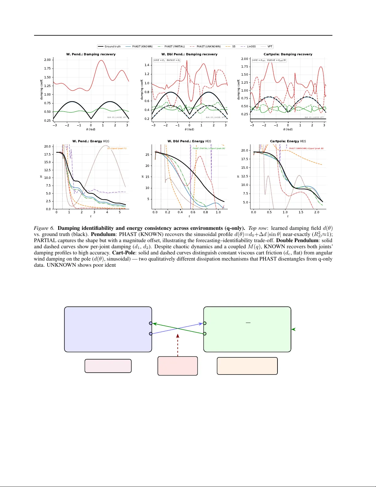
PHAST : P ort-Hamiltonian Ar chitecture f or Structur ed T emporal Dynamics F orecasting Shubham Bhardwaj 1 2 Chandrajit Bajaj 1 Abstract Real physical systems are dissipativ e—a pendulum slows, a circuit loses char ge to heat—and forecasting their dynamics from partial observations is a central challenge in scientiﬁc machine learning. W e address the position- only (q-only) problem: gi ven only generalized positions q t at discrete times (momenta p t latent), learn a structured model that (a) produces stable long-horizon forecasts and (b) recov ers physically meaningful parameters when sufﬁcient structure is pro vided. The port-Hamiltonian framew ork makes the conserv ativ e–dissipative split e xplicit via ˙ x = ( J − R ) ∇ H ( x ) , guaranteeing dH /dt ≤ 0 when R ⪰ 0 . W e introduce PHAST (Port-Hamiltonian Archi- tecture for Structured T emporal dynamics), which decomposes the Hamiltonian into potential V ( q ) , mass M ( q ) , and damping D ( q ) across three knowledge re gimes (KNO WN, P AR TIAL, UNKNOWN), uses ef ﬁcient lo w-rank PSD/SPD parameterizations, and adv ances dynamics with Strang splitting. Across thirteen q-only benchmarks spanning mechanical, electrical, molecular , thermal, gravitational, and ecological systems, PHAST achiev es the best long-horizon forecasting among competitiv e baselines and enables physically meaningful parameter recovery when the regime provides suf ﬁcient anchors. W e sho w that identiﬁcation is fundamentally ill-posed without such anchors (gauge freedom), motiv ating a two-axis ev aluation that separates forecasting stability from identiﬁability . 1. Introduction Forecasting the future states of dynamical systems from observational data is a central problem in scientiﬁc machine learning. Physical systems span a wide spectrum of complexity: simple conservative systems (e.g., an undamped pendulum or a frictionless spring) preserv e total energy and trace closed orbits in phase space; dissipative systems (e.g., a pendulum slo wing due to air drag, an RLC circuit losing char ge to resistiv e heating) lose energy ov er time and con verge to ward attractors; and chaotic systems (e.g., a double pendulum, turb ulent ﬂuid ﬂows) exhibit sensiti ve dependence on initial conditions, making long-horizon prediction fundamentally difﬁcult. A practical forecasting framework must handle all three regimes—and, crucially , most real-world systems are dissipative : a swinging pendulum eventually stops, a robot arm loses ener gy through joint friction, and electrical circuits dissipate energy as heat. Problem setting . W e formalize the forecasting task in the position-only (q-only) setting: we observe only generalized positions q t at discrete times; momenta p t are latent and nev er measured. The goal is to learn a structured dynamical model from q-only data that (a) produces stable long-horizon open-loop forecasts and (b) when partial physics is a vailable, recov ers physically interpretable parameters (potential, mass, damping). Port-Hamiltonian framework. The port-Hamiltonian frame work ( V an Der Schaft & Jeltsema , 2014 ) provides a principled decomposition for dissipativ e systems: ˙ x = ( J − R ) ∇ H ( x ) + Gu, (1) where x = ( q , p ) denotes generalized coordinates and momenta. The term Gu represents external actuation: u is a generalized force (e.g., torque at a joint), and the port matrix G selects which de grees of freedom are actuated. The conjugate 1 Department of Computer Science, Oden Institute for Computational Engineering and Sciences, The Univ ersity of T exas at Austin, Austin, TX, USA 2 Mihawk.ai. Correspondence to: Shubham Bhardwaj < shubham.bhardwaj@ute xas.edu > . Pr eprint. F ebruary 23, 2026. 1 PHAST : P ort-Hamiltonian Architectur e for Structur ed T emporal Dynamics port output y port = G ⊤ ∇ H ( x ) is velocity-like for mechanical systems, and the product u ⊤ y port is the instantaneous power supplied to the system—the rate at which external work ﬂows in through the port. Our forecasting benchmarks have no external actuation, so we set u ≡ 0 throughout Sections 1–4; the forced form and its port structure become central in the Energy–Casimir control study (Sec. 3.5 ). In port-Hamiltonian form, dynamics decompose into energy geometry (via the mass tensor M ( q ) ), en vironmental structure (via the potential V ( q ) ), and dissipation ( D ( q ) ), enabling principled combinations of known physics and learned components (Sec. 1 ). For mechanical systems, the Hamiltonian takes the form H ( q , p ) = V ( q ) + T ( q , p ) with kinetic energy T ( q , p ) = 1 2 p ⊤ M ( q ) − 1 p , where M ( q ) ≻ 0 is the generalized mass (inertia) tensor—it induces a Riemannian metric on conﬁguration space under which free trajectories are geodesics—and we deﬁne the generalized velocity v := ∇ p H ( q , p ) = M ( q ) − 1 p . In our experiments we use a separable constant-mass approximation M ( q ) ≈ M for ef ﬁciency (Sec. 1 ), but the architecture supports the general conﬁguration-dependent case (Appendix H.2 ). The operator J = − J ⊤ encodes conservati ve energy exchange via the canonical symplectic structure. Dissipation is introduced through a structured operator R ( q ) =  0 0 0 D ( q )  , D ( q ) = D ( q ) ⊤ ⪰ 0 , so that damping acts only on the momentum dynamics. This corresponds to standard mechanical dissipation, where friction affects generalized v elocities but not positions. W ith the canonical symplectic structure and the block-diagonal dissipation, the dynamics decompose explicitly as ˙ q = ∇ p H ( q , p ) , (2) ˙ p = −∇ q H ( q , p ) − D ( q ) ∇ p H ( q , p ) . (3) This structure yields an explicit ener gy balance: ˙ H ( x ) = ∇ H ( x ) ⊤ ( J − R ) ∇ H ( x ) = −∇ H ( x ) ⊤ R ∇ H ( x ) ≤ 0 , (4) since ∇ H ⊤ J ∇ H = 0 by ske w-symmetry . As a result, the system is passiv e by construction, guaranteeing non-increasing energy re gardless of the speciﬁc parameterization of H ( x ) . Oscillatory dynamics. In the conserv ative case ( D = 0 ), the dynamics reduce to ˙ x = J ∇ H ( x ) ; linearizing around an elliptic equilibrium (e.g., a local minimum of the potential with M ≻ 0 ) yields purely imaginary eigen values (phase-space rotations), corresponding to oscillatory e xchange between kinetic and potential ener gy . Adding D ⪰ 0 shifts eigen values into the closed left half-plane (e.g., − σ ± iω ), yielding damped oscillations; Appendix A.4 provides a concise linear-algebra statement and proof for the linearized model ˙ x = ( J − R ) Qx ( Mehl et al. , 2018 ). This work develops neural architectures that respect this structure (Appendix A.2 ). Motivation. W e are motiv ated by three con verging observ ations: (i) Physics-informed networks like HNNs ( Gre ydanus et al. , 2019 ) and LNNs ( Cranmer et al. , 2020 ) show that structure improv es generalization, but they assume purely conservati ve systems ( R = 0 ). (ii) State-space models like S5 ( Smith et al. , 2023 ), LinOSS ( Hasani et al. , 2024 ), and D-LinOSS ( Boyer et al. , 2025 ) achiev e efﬁciency but typically do not provide e xplicit physical guarantees—e.g., they do not expose an explicit port-Hamiltonian decomposition or a passi vity certiﬁcate. (iii) Structure-preserving networks lik e V olume-Preserving T ransformers ( Brantner et al. , 2024 ) enforce geometric constraints such as v olume preserv ation, i.e., their one-step map ϕ ∆ t : x t 7→ x t +1 has unit Jacobian determinant det( ∂ ϕ ∆ t /∂ x t ) = 1 , which is naturally aligned with conservati ve, di ver gence-free dynamics. Howe ver , they do not pro vide an explicit dissipation mechanism or a certiﬁcate of passivity for lossy systems, and strictly v olume-preserving maps cannot represent generic dissipati ve ﬂows that contract phase-space volume. W e propose PHAST (Port-Hamiltonian with Strang Splitting), which properly models both the conservati ve ( J ) and dissipativ e ( R ) components. The key insight is that the port-Hamiltonian structure provides passi vity r e gar dless of how the components are parameterized: whether the potential V ( q ) , mass M ( q ) , and damping D ( q ) are structured functions or neural networks, the continuous-time dynamics satisfy dH /dt ≤ 0 by construction. PHAST addresses the q-only problem via a three-stage pipeline: a causal velocity observer reconstructs ˆ ˙ q from position history , a canonicalizer maps to phase state ( q , ˆ p ) , and the port-Hamiltonian core integrates forw ard with Strang splitting. Giv en a short burn-in window q 0: K − 1 , PHAST rolls out open-loop; Section 3 details the components. 2 PHAST : P ort-Hamiltonian Architectur e for Structur ed T emporal Dynamics Regime Domain System For ecast q V ( q ) : landscape M ( q ) : geometry D ( q ) : dissipation Ident.? K N O W N Mechanics Pendulum Angle θ ( t ) − g cos θ Scalar m Air drag d ( θ ) Y es Mechanics Spring–mass Displacement x ( t ) 1 2 kx 2 Scalar m V iscous b ˙ x Y es Molecular Lennard–Jones Positions r i ( t ) 4 ϵ [( σ /r ) 12 − ( σ /r ) 6 ] Diagonal mI Solvent friction γ I Y es Electrical RLC circuit Charge q C ( t ) q 2 / 2 C Inductance L Resistance R Y es Thermal Heat exchange T emperature T ( t ) 1 2 c T 2 Time constant τ Heat loss κ Y es P ART I A L Mechanics Pendulum (unk. m ) Angle θ ( t ) − g cos θ (given) mI (learn m ) Learned (bounded) Y es Robotics Robot arm Joint angles θ i ( t ) Gravity regressor CAD inertia template Joint friction (learned) Y es Astrophysics N-body gravity Positions r i ( t ) − P i 0 ), this yields ˙ H cl ≤ − d inj ∥ y p ∥ 2 ≤ 0 , guaranteeing asymptotic con vergence to the minimum of H cl at q ⋆ . For ced dynamics mode. In the experiments of Appendix 5 we additionally inject an exogenous signal v ext (for excitation or tracking), setting v ( t ) = v ext ( t ) − d inj ˆ y ( t ) , (25) where ˆ y is the (possibly estimated) port output. Substituting ( 23 )–( 25 ) into the po wer balance giv es y ⊤ p u p + y ⊤ c u c = y ⊤ p v ext − d inj y ⊤ p ˆ y . (26) In the ideal case ˆ y ≡ y p , the closed-loop storage satisﬁes the forced passivity bound ˙ H cl ≤ y ⊤ p v ext − d inj ∥ y p ∥ 2 , (27) i.e. the closed loop is passiv e from v ext to y p with strict dissipation. The Casimir in variance is compatible with forced mode: v ext enters only through u p and does not alter the constraint u c = y p . 10 PHAST : P ort-Hamiltonian Architectur e for Structur ed T emporal Dynamics Q-only limitation. In q-only settings y p is not observed directly and must be replaced by an estimate ˆ y ≈ y p . The dissipati ve term then becomes − d inj y ⊤ p ˆ y , which can lose deﬁniteness when ˆ y  = y p : estimation error may inject or dissipate energy . This is the central partial-observability bottleneck for port-based control. Discrete-time implementation. Let q meas t denote q-only measurements and ˆ y t the online port estimate. The controller is implemented as u t = − y c ( ξ t ) + v ext ,t − d inj ˆ y t , (28) ξ t +1 = ξ t + ∆ t  ˆ y t + k ξ ( q meas t − ξ t )  , (29) where k ξ ≥ 0 is an optional predictor–corrector gain that corrects ξ drift under partial observability: when ˆ y = y p and k ξ =0 , the update reduces to a forward-Euler discretization of ˙ ξ = y p . All variants share the same ( k c , d inj , k ξ ) and forcing signal v ext ,t ; they dif fer only in how ˆ y t is produced online. Port-estimation v ariants. W e compare the same family of estimators as in the unforced setting (oracle/full-state, ﬁnite differences, ﬁxed-lag MAP smoothing, learned observer , etc.) and ev aluate stability and control-ef fort degradation as a function of port-estimation error (Appendix 5 ). 4. Experiments W e e valuate PHAST on q-only systems spanning conserv ative and dissipati ve dynamics across six physical domains. Our ev aluation separates two regimes with distinct goals: open-loop for ecasting (autonomous rollouts) to assess long-horizon stability and physical identiﬁability , and closed-loop contr ol (feedback) to assess whether the learned port-Hamiltonian structure remains useful under stabilization and to isolate the role of online port estimation under partial observability . 4.1. Open-loop for ecasting (q-only) 4 . 1 . 1 . E X P E R I M E N TA L S E T U P En vironments. W e ev aluate on thirteen q-only benchmarks spanning conservati ve and dissipative dynamics across six physical domains. Mechanical systems (eight benchmarks): single pendulum (conservati ve, constant damping, and position-dependent “windy” damping), a windy Cart-Pole on R × S 1 , harmonic oscillator (conservati ve and damped), and double pendulum (conservati ve and damped). Non-mechanical systems (ﬁve benchmarks cov ering all three knowledge regimes in T able 1 ): series RLC circuit (KNOWN), Lennard–Jones 3-particle cluster (KNO WN), coupled heat exchange (KNO WN), 3-body gravitational system (P AR TIAL), and Lotka–V olterra predator–prey (UNKNO WN). In all en vironments only conﬁgurations q t are observed; the simulator e volves trajectories from random initial conditions ( q 0 , p 0 ) . All models are trained as next-step predictors that map a short history of observed conﬁgurations to ˆ q t +1 ; PHAST internally uses the same history to infer a latent phase state via the FD+TCN observer (Sec. 3.1 ), while sequence baselines must implicitly learn any required state estimation. All forecasting benchmarks are unforced ( u = 0 in Eq. ( 1 ) ). For windy settings we use a position-dependent diagonal damping of the form d ( q ) = d 0 + ∆ d | sin q | (e.g., d 0 =0 . 3 , ∆ d =0 . 5 ), applied to the rele vant angular coordinate. Some benchmarks (Cart-Pole and Double Pendulum) have conﬁguration-dependent inertia M ( q ) in the simulator; unless otherwise stated, we use a separable constant-mass approximation for ef ﬁciency (Sec. 1 ) and study the nonseparable M ( q ) v ariant in Appendix H.2 . Appendix B provides detailed en vironment descriptions and Hamiltonians. Data protocol. T rajectories have length T =200 . W e use ∆ t =0 . 05 for single-pendulum en vironments, ∆ t =0 . 02 for Cart-Pole and Oscillator , and ∆ t =0 . 01 for Double Pendulum. For PHAST , we initialize the internal integrator step size to the en vironment timestep ∆ t and use a single integration substep per observ ation step ( L =1 ); unless otherwise stated, the internal timestep is learnable. Dataset sizes are N train / N val / N test = 1000 / 200 / 200 . Unless otherwise noted, tables report mean ± std ov er 5 random model seeds using a ﬁxed dataset shared across models, and all runs are e xecuted on CPU for reproducibility . All models are trained for 50 epochs; complete hyperparameters are provided in Appendix E . T raining and model selection. All methods use the same optimizer and schedule: AdamW (weight decay 10 − 5 ) with a cosine learning-rate schedule. W e select the model parameters with lowest v alidation MSE (ev aluated ev ery 10 epochs) and report test metrics for that selection. 11 PHAST : P ort-Hamiltonian Architectur e for Structur ed T emporal Dynamics Rollout MSE → Identiﬁability (damping R 2 ↑ ) Ideal P AR TIAL KNOWN UNKNOWN D-LinOSS S5 GR U more structure F igure 4. T wo-axis ev aluation (open-loop, conceptual). Forecasting accuracy (low rollout MSE) and physical identiﬁability (high damping R 2 ) are distinct objectiv es; model/regularizer choices induce trade-offs. Baselines. W e compare against GRU ( Cho et al. , 2014 ), S5 ( Smith et al. , 2023 ), LinOSS ( Hasani et al. , 2024 ), D- LinOSS ( Boyer et al. , 2025 ), a T ransformer ( V aswani et al. , 2017 ), and a V olume-Preserving Transformer (VPT) ( Brantner et al. , 2024 ). W e report trainable parameter counts for all methods; parameter matching is treated as an experimental control rather than an assumption. All baselines are trained and ev aluated as causal seq2seq predictors that map a q-only history to the next conﬁguration ( q 0: t 7→ ˆ q t +1 ); they do not use an e xplicit observer/canonicalizer pipeline. 4 . 1 . 2 . E V A L U A T I O N P RO T O C O L : T W O A X E S Forecasting accurac y and physical parameter recov ery are distinct objectiv es. A model may achiev e good rollouts by using D ( q ) as a “stabilizer” rather than learning true physical damping. Con versely , recovering true D ( q ) does not guarantee good open-loop rollouts if V ( q ) or M have errors. W e therefore e valuate open-loop performance along two ax es (Fig. 4 ): Axis 1: F orecasting stability . F or angular coordinates we report one-step wrapped-angle MSE and long-horizon open-loop rollout error at horizon H =100 with burn-in conte xt K =10 . For Euclidean q-only en vironments we report standard MSE and rollout MSE at H =100 . For mixed manifolds (Cart-Pole) we report a mixed-manifold rollout MSE at H =100 that av erages translation MSE and wrapped-angle MSE. All models are ev aluated in open-loop (autoregressi ve) mode; PHAST additionally supports takeov er rollouts (burn-in then integrate; Appendix C.3 ) as a diagnostic of the learned dynamics. Axis 2: Identiﬁability . When a model exposes an explicit damping ﬁeld D ( q ) , we report damping recov ery via R 2 and MAE. W e also report an ener gy-consistency diagnostic on open-loop rollouts (ener gy-budget residual at H =100 ), computed from ﬁnite-difference velocity estimates and the benchmark’ s simulator damping law D env ( · ) for expected dissipation (Appendix F ). Precise metric deﬁnitions (including rollout protocol and the discrete energy-b udget residual) are provided in Appendix F . Regime-speciﬁc expectations. In KNO WN/P AR TIAL re gimes, physics-calibrated damping bounds (e.g., P i β i ( q ) ≤ ¯ β ≈ ∆ d ) can improve identiﬁability without destabilizing rollouts (T able 6 ; Appendix T able 31 ). In UNKNOWN, damping bounds can re veal a forecasting–identiﬁability trade-of f unless additional anchors break gauge freedoms (Appendix T able 32 ). Open-loop error sources & diagnostics. W e report rollout error (stability), damping R 2 (identiﬁability), energy-budget residual, and discrete-time passi vity violations. Appendix F .1 provides the q-only computation graph and diagnostic interpretations (autoregressi ve vs. takeov er, step-size/substepping, damping bounds, and time-scale ambiguity). 4 . 1 . 3 . M A I N O P E N - L O O P R E S U LT S Main qualitative results. W e present qualitativ e results across three benchmarks that probe complementary aspects of dissipative dynamics learning (Fig. 5 ). The W indy P endulum (1 DOF , S 1 ) is the simplest: constant mass, a single position-dependent damping coef ﬁcient d ( θ ) , and regular oscillatory trajectories. It tests whether a model can learn basic dissipativ e Hamiltonian dynamics from positions alone. The W indy Double P endulum (2 DOF , T 2 ) escalates difﬁculty 12 PHAST : P ort-Hamiltonian Architectur e for Structur ed T emporal Dynamics 0 2 4 t 3 2 1 0 1 2 ( r a d ) bur n-in S5, LinOS S +1 clipped W . P e n d . : ( t ) 2 1 0 1 2 ( r a d ) 4 2 0 2 4 6 p clipped: S5, LinOS S, VPT W . P e n d . : P h a s e ( q , p ) 0.00 0.25 0.50 0.75 1.00 t 2.5 2.0 1.5 1.0 0.5 0.0 0.5 1 ( r a d ) bur n-in S5, LinOS S +1 clipped W . D b l P e n d . : 1 ( t ) 2 1 0 1 ( r a d ) 4 5 6 7 8 9 p 1 clipped: PHAST (KNOWN), PHAST (P ARTIAL), PHAST (UNKNOWN) +3 W . D b l P e n d . : P h a s e ( q , p ) 0.00 0.25 0.50 0.75 1.00 t 3 2 1 0 1 2 2 ( r a d ) bur n-in LinOS S, VPT clipped W . D b l P e n d . : 2 ( t ) 2 0 2 2 ( r a d ) 0 2 4 6 8 10 p 2 clipped: S5, LinOS S, VPT W . D b l P e n d . : P h a s e ( q , p ) 0.0 0.5 1.0 1.5 2.0 t 3 2 1 0 1 2 ( r a d ) bur n-in S5, LinOS S +1 clipped C a r t p o l e : ( t ) 2 0 2 ( r a d ) 2 1 0 1 2 3 4 5 p clipped: S5, LinOS S, VPT C a r t p o l e : P h a s e ( q , p ) Gr ound truth PHAST (KNOWN) PHAST (P AR TIAL) PHAST (UNKNOWN) S5 LinOSS VPT F igure 5. Open-loop rollouts and phase-space portraits across thr ee dissipativ e benchmarks (q-only). T op row : a single test trajectory is teacher -forced through a short b urn-in windo w (gre y region, vertical dashed line), then predicted open-loop for H =100 steps. Column 1 (W indy Pendulum, θ ): the simplest system — a single angle with position-dependent damping. PHAST (KNO WN/P AR TIAL) tracks the decaying oscillation almost exactly; all three baselines div erge within a few periods. Columns 2–3 (W indy Double Pendulum, θ 1 and θ 2 ): a chaotic 2-DOF system with coupled conﬁguration-dependent inertia M ( q ) . This is the hardest benchmark: small errors grow exponentially , yet PHAST maintains trajectory coherence on both joints f ar longer than baselines. Showing both angles re veals that the model captures inter-joint coupling, not just marginal statistics. Column 4 (W indy Cart-Pole, θ ): a mixed-manifold system ( R × S 1 ) with two qualitatively different damping mechanisms (constant cart friction + angular wind damping). PHAST (P AR TIAL) achieves the tightest tracking here. Bottom r ow : canonical phase-space portraits ( θ , p ) with p = M ( q ) ˙ q during the open-loop segment. Momentum is latent in the q-only setting: for PHAST , ˙ q comes from the learned FD+TCN observ er (Sec. 3 ); for baselines, ˙ q is approximated by ﬁnite differences. The closed orbits visible for PHAST conﬁrm that the model has learned physically consistent Hamiltonian structure, whereas baseline phase portraits collapse or spiral outward. sharply: the dynamics are chaotic, the mass matrix M ( q ) couples the two links through cos( θ 1 − θ 2 ) , and each joint has independent wind damping. Small prediction errors grow e xponentially , making this the hardest forecasting challenge in our suite. The W indy Cart-P ole (2 DOF , R × S 1 ) represents a dif ferent axis of dif ﬁculty: a mix ed manifold (translation × rotation), conﬁguration-dependent inertia M ( q ) , and two qualitatively differ ent damping mechanisms — constant viscous cart friction and position-dependent angular wind damping on the pole. Full forecasting tables across all thirteen q-only benchmarks are reported in Appendix G . T able 4 provides a compact summary across the full benchmark suite (see also Fig. 2 in Sec. 1 for a visual ov ervie w). Because the Double Pendulum and Cart-Pole hav e nonseparable Hamiltonians ( M ( q )  = const ), we use the implicit-midpoint integrator for all PHAST curves in the multi-en vironment ﬁgures. Appendix H.2 further discusses the nonseparable mass variant. T able 3 sho ws that PHAST achieves strong long-horizon stability on W indy Cart-Pole. Figure 6 shows the learned damping proﬁles and energy traces across all three systems, illustrating the forecasting–identiﬁability trade-of f: T able 5 highlights the two-axis nature of the problem: in the Windy setting, the KNO WN regime recov ers a physically meaningful damping ﬁeld, P AR TIAL becomes identiﬁable once we impose a physics-calibrated magnitude bound ¯ β on D ( q ) , and UNKNO WN still exhibits a forecasting–identiﬁability trade-of f without additional anchors (Appendix F ). Appendix H makes this trade-of f explicit: T able 6 compares bounded vs. unbounded damping in the P AR TIAL regime, sho wing that without the bound the model can achie ve accurate rollouts while learning a physically meaningless damping ﬁeld ( R 2 D ≪ 0 ). T akeo ver rollouts 13 PHAST : P ort-Hamiltonian Architectur e for Structur ed T emporal Dynamics T able 3. Q-only open-loop for ecasting (Cart-Pole). Mean ± std of mixed-manifold rollout MSE at horizon H =100 o ver 5 seeds. The mixed metric a verages translation MSE and wrapped-angle MSE (Appendix F ). Lo wer is better . Model Params Cart-Pole (windy) PHAST (ours) PHAST (KNO WN) 3,589 0 . 063 ± 0 . 019 PHAST (P AR TIAL) 14,283 0 . 083 ± 0 . 022 PHAST (UNKNO WN) 14,290 0 . 109 ± 0 . 022 S5 (best baseline) 17,218 0 . 431 ± 0 . 077 T able 4. Suite summary across thirteen q-only benchmarks. For each benchmark, we report the best PHAST regime and the best baseline (mean ± std over 5 seeds). The ﬁrst eight rows use rollout MSE at horizon H =100 ; the last ﬁve report next-step MSE (T ables 20 – 24 ). Gains are per-ro w ratios and are not directly comparable across en vironments. Benchmark Best PHAST Best baseline Gain Mechanical systems (r ollout MSE at H =100 ) Pendulum (cons) 0 . 680 ± 0 . 043 (P AR TIAL) 2 . 320 ± 0 . 224 (Transformer) 3 . 4 × Pendulum (damped) 0 . 017 ± 0 . 005 (KNOWN) 0 . 450 ± 0 . 241 (D-LinOSS) 26 . 5 × Pendulum (windy) 0 . 092 ± 0 . 014 (P AR TIAL) 0 . 435 ± 0 . 239 (D-LinOSS) 4 . 7 × Cart-Pole (windy) 0 . 063 ± 0 . 019 (KNOWN) 0 . 431 ± 0 . 077 (S5) 6 . 8 × Oscillator (cons) 0 . 0010 ± 0 . 0002 (KNOWN/P AR TIAL) 1 . 087 ± 0 . 299 (Transformer) 1 . 1 × 10 3 Oscillator (damped) 0 . 0011 ± 0 . 0003 (P AR TIAL) 0 . 926 ± 0 . 254 (Transformer) 8 . 4 × 10 2 Double pendulum (cons) 0 . 402 ± 0 . 047 (P AR TIAL) 0 . 618 ± 0 . 028 (S5) 1 . 5 × Double pendulum (damped) 0 . 320 ± 0 . 032 (P AR TIAL) 0 . 630 ± 0 . 031 (S5) 2 . 0 × Non-mechanical systems (next-step MSE) RLC circuit (KNOWN) 2 . 63 × 10 − 5 (UNKNOWN) 4 . 81 × 10 − 4 (Transformer) 18 × LJ-3 cluster (KNOWN) 4 . 59 × 10 − 10 (P AR TIAL) 2 . 05 × 10 − 4 (S5) 4 . 5 × 10 5 Heat exchange (KNO WN) 2 . 42 × 10 − 6 (KNOWN) 4 . 46 × 10 − 4 (LinOSS) 1 . 8 × 10 2 N-body gravity (P AR TIAL) 4 . 27 × 10 − 8 (P AR TIAL) 1 . 83 × 10 − 3 (Transformer) 4 . 3 × 10 4 Predator–prey (UNKNO WN) 0 . 0199 (UNKNOWN) 0 . 179 (Transformer) 9 . 0 × (burn-in then inte grate) can improve with better identiﬁability , b ut remain sensiti ve to single-shot momentum inference at the context boundary; we therefore treat takeo ver as a diagnostic rather than the primary q-only comparison metric. Additional studies (open-loop). Appendix H reports additional open-loop ablations (integrator choices, observer capacity , and damping constraints, including ¯ β sweeps) and a full-state comparison. 4.2. Closed-loop control (Ener gy–Casimir stabilization) Demarcation from open-loop. Open-loop forecasting e v aluates autonomous rollouts ( u = 0 ) and physical identiﬁability of learned ﬁelds. Closed-loop ev aluation instead probes whether the learned pH structure supports passivity-based stabilization under feedback. In q-only settings, closed-loop performance depends critically on the quality of the online port/v elocity estimate used for damping injection. Scope (closed-loop). Throughout this subsection we keep the controller structure and gains ﬁxed and vary only the port/velocity estimate ˆ y used for damping injection and (optionally) for the controller-state update. Unless stated otherwise, the plant is the true pendulum integrated by RK4. Setup and controller . W e e valuate stabilization on a single-de gree-of-freedom pendulum plant with state x = ( q , p ) and q-only measurements q meas t = q t + ϵ t . The Energy–Casimir -style controller maintains an internal state ξ and uses a port estimate ˆ y t ≈ y p ( t ) (which reduces to ˆ y t = ˆ ˙ q t for the pendulum): u t = − k c ( ξ t − q ⋆ ) − d inj ˆ y t , (30) ξ t +1 = ξ t + ∆ t  ˆ y t + k ξ ( q meas t − ξ t )  , (31) where the k ξ term is a predictor–corrector measurement correction that reduces ξ drift under noisy q-only feedback. When k ξ = 0 and ˆ y = y p , the update reduces to a discrete approximation of ˙ ξ = y p . 14 PHAST : P ort-Hamiltonian Architectur e for Structur ed T emporal Dynamics T able 5. Windy Pendulum (q-only) identiﬁability and energy consistency . Mean ± std o ver 5 seeds (same setup as T able 17 ). Baselines do not expose a damping ﬁeld, so damping reco very metrics are not applicable. Model W rapMSE roll θ ( H =100) ↓ R 2 D ↑ MAE D ↓ EbudRes roll ( H =100) ↓ Params PHAST (KNOWN) 0 . 106 ± 0 . 020 0 . 996 ± 0 . 004 0 . 007 ± 0 . 004 1 . 56 ± 0 . 02 3,364 PHAST (P AR TIAL) 0 . 092 ± 0 . 014 0 . 654 ± 0 . 077 0 . 063 ± 0 . 011 1 . 50 ± 0 . 04 13,736 PHAST (UNKNOWN) 0 . 298 ± 0 . 048 − 96 . 546 ± 15 . 897 1 . 343 ± 0 . 115 2 . 58 ± 0 . 19 13,738 GR U 1 . 796 ± 0 . 625 — — 12 . 34 ± 6 . 58 37,889 S5 0 . 600 ± 0 . 047 — — 11 . 71 ± 2 . 91 17,089 LinOSS 1 . 458 ± 0 . 324 — — 56 . 14 ± 37 . 41 17,089 D-LinOSS 0 . 435 ± 0 . 239 — — 6 . 86 ± 1 . 14 33,793 Transformer 0 . 824 ± 0 . 134 — — 7 . 71 ± 0 . 63 100,161 VPT 2 . 218 ± 0 . 135 — — 40 . 48 ± 8 . 04 16,833 T able 6. P AR TIAL regime: effect of bounding total damping strength (Windy P endulum, q-only). Mean ± std over 5 seeds on CPU (same data protocol as Sec. 4.1.1 ). W ithout the bound, damping becomes an “error sink” and is non-identiﬁable ( R 2 D ≪ 0 ) e ven when rollouts are accurate; bounding P r i =1 β i ( q ) recovers a physically meaningful damping ﬁeld. Damping cap WrapMSE θ (100) ↓ R 2 D ↑ MAE D ↓ EbudRes(100) ↓ Unbounded 0 . 059 ± 0 . 007 − 90 . 15 ± 6 . 14 1 . 326 ± 0 . 044 1 . 50 ± 0 . 03 P i β i ( q ) ≤ 0 . 5 0 . 071 ± 0 . 004 0 . 703 ± 0 . 072 0 . 061 ± 0 . 010 1 . 58 ± 0 . 04 Closed-loop protocol and metrics. W e e valuate N rollouts from random initial conditions ov er horizon T ctl and report: (i) success rate (fraction of trials that con ver ge to the target), (ii) ﬁnal wrapped-angle error , (iii) control ef fort P T ctl − 1 t =0 ∥ u t ∥ 2 2 , and (i v) port-estimation error E t ∥ ˆ y t − y p ( t ) ∥ when y p is av ailable in simulation. Precise thresholds, horizons, and noise settings follow Appendix 5 . Port-estimation variants. W e compare ﬁv e Energy–Casimir variants that share the same shaping gain k c , damping- injection gain d inj , and drift-correction gain k ξ , dif fering only in ho w ˆ y t is obtained online: (i) oracle/full-state, (ii) ﬁnite differences, (iii) ﬁxed-lag MAP smoothing (label-free), (iv) FD+TCN observer trained of ﬂine with noise augmentation, and (v) PHAST -trained observer trained only through next-step prediction. Appendix 5 reports additional control ablations (noise mismatch, near-stable re gime, and model-based velocity from learned ˆ H ). Closed-loop r esults (summary). Sec. 5 shows that PHAST models support passi vity-based stabilization: using the learned PHAST Hamiltonian to compute the port output ˆ y = ∂ ˆ H /∂ p achiev es 100% stabilization success with lower control effort than oracle velocities (245 vs. 263), indicating the learned energy landscape is accurate enough for feedback. Under q-only sensing, the bottleneck shifts to port/velocity estimation quality rather than model accurac y; noise-aw are observers reduce control effort by ∼ 9 × compared to ﬁnite differences. 5. Energy-Casimir Contr ol Energy–Casimir control is a passi vity-based approach for stabilizing port-Hamiltonian plants by interconnecting the plant with a dynamic controller and shaping a closed-loop storage function (Hamiltonian plus Casimir). Although PHAST is ev aluated primarily as an open-loop forecaster in the main paper , port-Hamiltonian models are often used in feedback settings. W e include this study to (i) show a minimal closed-loop wiring compatible with the port v ariables in Sec. 3.1 , and (ii) isolate a practical bottleneck in q-only control: the controller requires the v elocity-like port output y p = y port (for torque actuation, y p = ˙ q ), which must be estimated online from noisy position measurements. Closed-loop scope. W e e valuate Energy–Casimir stabilization under q-only feedback. Across all control experiments we keep the controller structure and gains ( k c , d inj , k ξ ) ﬁxed and v ary only the online port estimate ˆ y ≈ y p used for damping injection (and, when stated, in the ξ update). Unless stated otherwise, the plant is the true pendulum integrated by RK4. What is a Casimir function? A Casimir function C ( z ) is a structural in variant of a port-Hamiltonian system: it satisﬁes ∇C ∈ ker J ⊤ cl ∩ ker R cl , so it is conserved by the interconnection structure regardless of the energy function. For the mechanical plant–controller pair , C ( q , ξ ) = q − ξ acts as a “conﬁguration lock”: the interconnection forces the controller state ξ to track the plant position q at all times (Sec. 3.5 ). 15 PHAST : P ort-Hamiltonian Architectur e for Structur ed T emporal Dynamics 3 2 1 0 1 2 3 ( r a d ) 0.25 0.50 0.75 1.00 1.25 1.50 1.75 2.00 damping coeff . N/A : S5, LinOS S, VPT W . Pend.: Damping recovery 0 1 2 3 4 5 t 0.0 2.5 5.0 7.5 10.0 12.5 15.0 17.5 20.0 H S5 clipped (peak 71) W . P e n d . : E n e r g y H ( t ) 3 2 1 0 1 2 3 ( r a d ) 0.2 0.4 0.6 0.8 1.0 1.2 1.4 damping coeff . s o l i d = d 1 , d a s h e d = d 2 N/A : S5, LinOS S, VPT W . Dbl Pend.: Damping recovery 0.0 0.2 0.4 0.6 0.8 1.0 t 5 10 15 20 25 H PHAST (P ARTIAL) clipped (peak 26) W . D b l P e n d . : E n e r g y H ( t ) 3 2 1 0 1 2 3 ( r a d ) 0.25 0.50 0.75 1.00 1.25 1.50 1.75 2.00 damping coeff . s o l i d = d c a r t , d a s h e d = d p o l e ( ) N/A : S5, LinOS S, VPT Cartpole: Damping recovery 0.0 0.5 1.0 1.5 2.0 t 5.0 7.5 10.0 12.5 15.0 17.5 20.0 H PHAST (UNKNOWN) clipped (peak 28) C a r t p o l e : E n e r g y H ( t ) Gr ound truth PHAST (KNOWN) PHAST (P AR TIAL) PHAST (UNKNOWN) S5 LinOSS VPT F igure 6. Damping identiﬁability and energy consistency across en vironments (q-only). T op r ow : learned damping ﬁeld d ( θ ) vs. ground truth (black). P endulum : PHAST (KNO WN) recovers the sinusoidal proﬁle d ( θ )= d 0 +∆ d | sin θ | near-e xactly ( R 2 D ≈ 1 ); P AR TIAL captures the shape but with a magnitude of fset, illustrating the forecasting–identiﬁability trade-off. Double Pendulum : solid and dashed curves show per-joint damping ( d 1 , d 2 ). Despite chaotic dynamics and a coupled M ( q ) , KNOWN recov ers both joints’ damping proﬁles to high accuracy . Cart-Pole : solid and dashed curves distinguish constant viscous cart friction ( d c , ﬂat) from angular wind damping on the pole ( d ( θ ) , sinusoidal) — two qualitativ ely different dissipation mechanisms that PHAST disentangles from q-only data. UNKNOWN shows poor identiﬁability across all systems ( R 2 D ≪ 0 ; T able 4 ). Baselines do not expose explicit damping ﬁelds (marked N/A). Bottom r ow : total energy H ( t ) during open-loop rollouts. In a dissipative system, ener gy must monotonically decrease; this is a necessary physical consistency check. PHAST (P AR TIAL) most closely tracks the ground-truth energy decay across all three systems. Baselines either di ver ge (energy blo wup) or collapse to zero, both indicating physically inconsistent dynamics. For PHAST , energy is computed using the observ er’ s learned velocity; for baselines, via ﬁnite dif ferences. Plant (pH) ˙ x = ( J p − R p ) ∇ H p + G p u p y p = G ⊤ p ∇ H p (velocity-like; y p = ˙ q for collocated) u p y p Controller (pH) H c ( ξ ) = k c 2 ( ξ − q ⋆ ) 2 ˙ ξ = u c y c = ∇ H c ( ξ ) (q-only: ˙ ξ = u c + k ξ ( ˜ q − ξ ) ) u c y c q ⋆ u c = y p u p = − y c + v Damping injection v = v ext − d inj ˆ y q-only: ˆ y ≈ y p v Casimir: C = q − ξ inv ariant when u c = y p = ˙ q Power balance y ⊤ p u p + y ⊤ c u c = y ⊤ p v ( = 0 when v =0 : no energy created) F igure 7. Energy–Casimir control as port-Hamiltonian interconnection. The plant (blue, left) and controller (green, right) are pH systems coupled through po wer ports: u c = y p feeds plant velocity to the controller, u p = − y c + v returns the shaped restoring force plus an auxiliary channel v . When v =0 the cross-power cancels ( y ⊤ p u p + y ⊤ c u c = 0 ), and the Casimir C = q − ξ is in variant. Damping injection v = − d inj ˆ y (red, dashed) ensures ˙ H cl ≤ 0 ; in q-only settings ˆ y ≈ y p is estimated, so estimation error can break e xact power balance. Having established the theoretical framework in Sec. 3.5 , we now e v aluate it experimentally . All experiments use the forced-dynamics mode of the Ener gy–Casimir controller (Eqs. 28 – 29 ) on a single-de gree-of-freedom pendulum. For the 16 PHAST : P ort-Hamiltonian Architectur e for Structur ed T emporal Dynamics T able 7. Energy–Casimir contr ol on the true pendulum (q-only sensing). Mean over 100 trials (5 regimes × 20). All methods use the same predictor–corrector ξ update ( k ξ = 5 ). σ Method V elocity estimate Success ↑ Final error ↓ Effort ↓ | ˆ ˙ q − ˙ q | ↓ 0.00 Oracle oracle 1.00 1 . 31 × 10 − 4 262.9 0.000 0.00 Finite differences FD 1.00 1 . 21 × 10 − 4 268.6 0.007 0.00 MAP smoother MAP smoother 1.00 1 . 16 × 10 − 4 268.6 0.007 0.00 FD+TCN observer FD+TCN 1.00 1 . 03 × 10 − 3 270.7 0.008 0.00 PHAST -trained observ er PHAST observer 1.00 5 . 71 × 10 − 3 272.4 0.019 0.01 Oracle oracle 1.00 5 . 49 × 10 − 3 262.9 0.000 0.01 Finite differences FD 1.00 1 . 67 × 10 − 2 342.2 1.117 0.01 MAP smoother MAP smoother 1.00 1 . 17 × 10 − 2 324.8 0.133 0.01 FD+TCN observer FD+TCN 1.00 2 . 39 × 10 − 2 335.5 0.172 0.01 PHAST -trained observ er PHAST observer 1.00 1 . 93 × 10 − 2 327.7 0.979 pendulum with collocated torque actuation, y p = ˙ q , so the port estimate reduces to ˆ y = ˆ ˙ q . MAP smoother observer (label-free). F or the MAP smoother baseline, we estimate ˆ ˙ q t by MAP smoothing over a ﬁxed-lag windo w of length w (with w ≥ 2 ) of q-only measurements q meas t − w +1: t . W e unwrap the angles within the window (integrating wrapped increments) and solv e the con vex quadratic problem q smooth ∈ arg min q w − 1 X s =0 1 σ 2   q s − q meas s   2 2 + w − 3 X s =0 1 ∆ t 4 σ 2 a   q s +2 − 2 q s +1 + q s   2 2 , (32) which corresponds to a Gaussian measurement model and a Gaussian prior on discrete acceleration. W e then take a backward difference on the smoothed sequence: ˆ ˙ q t = q smooth w − 1 − q smooth w − 2 ∆ t . (33) This baseline requires only q meas and the assumed noise scales ( σ, σ a ) ; it does not use ˙ q supervision. Unless otherwise stated, we ﬁx σ a = 10 . 0 for all MAP results. Main r esults. T able 7 summarizes the overall results under (i) no measurement noise and (ii) moderate q-only measurement noise σ = 0 . 01 . Under noise, ﬁnite differences incur large v elocity error and increased control effort; the learned FD+TCN observer reduces velocity error by ∼ 6–7 × while preserving con vergence. The PHAST -trained observer also preserves con vergence at σ = 0 . 01 , but its velocity estimate remains noisy (closer to ﬁnite dif ferences), which increases damping- injection effort near the tar get. A simple MAP smoother provides a competitiv e label-free baseline, reducing velocity error and ﬁnal error without requiring ˙ q supervision. This emphasizes that closed-loop performance hinges on the quality of the port output estimate y = ˙ q . Model-based velocity fr om a learned PHAST model (full-state). T o isolate the ef fect of model mismatch from partial observability , we also ev aluate a controller that uses a learned PHAST Hamiltonian to form the port output estimate ˆ y = ∂ ˆ H /∂ p from the observed state ( q , p ) . T able 8 shows that this model-based velocity estimate is accurate enough to preserve stability , supporting the use of PHAST -learned dynamics for control when full state is available. Near -target efﬁciency under noisy q-only feedback. The strongest effect of learning a noise-a ware observ er is visible near the target, where ﬁnite dif ferences can inject high-frequency damping torques. T able 9 reports the near -stable regime ( 20 trials) under σ = 0 . 01 . Observer -noise match ablation (limiting factor). T o isolate the key f ailure mode under noisy q-only feedback, we train the FD+TCN observer under dif ferent noise distributions and e valuate at σ = 0 . 01 . T able 10 sho ws that noise-matching 17 PHAST : P ort-Hamiltonian Architectur e for Structur ed T emporal Dynamics T able 8. Energy–Casimir with PHAST -based velocity (q,p observed). Mean over 100 trials (5 regimes × 20). Both methods use the same predictor–corrector ξ update ( k ξ = 5 ). σ Method V elocity estimate Success ↑ Final error ↓ Effort ↓ | ˆ ˙ q − ˙ q | ↓ 0.00 Oracle oracle 1.00 1 . 31 × 10 − 4 262.9 0.000 0.00 PHAST model-based ∂ ˆ H /∂ p 1.00 5 . 46 × 10 − 5 245.0 0.011 0.01 Oracle oracle 1.00 5 . 49 × 10 − 3 262.9 0.000 0.01 PHAST model-based ∂ ˆ H /∂ p 1.00 5 . 32 × 10 − 3 245.1 0.011 T able 9. Near -stable regime ( σ = 0 . 01 ). Learning a noise-aware q-only observ er reduces control effort near the target by ∼ 9 × vs. ﬁnite differences. Method Final error ↓ Ef fort ↓ | ˆ ˙ q − ˙ q | ↓ Oracle 0.0041 6.3 0.000 Finite differences 0.0170 80.1 1.117 MAP smoother 0.0133 10.3 0.095 FD+TCN observer 0.0137 8.6 0.130 PHAST -trained observer 0.0188 54.9 0.911 (or a narro w range anchored to deployment noise) is the dominant factor: training the observer at σ = 0 and deploying at σ = 0 . 01 recov ers neither accurate velocities nor low-ef fort behavior . T akeaway . These experiments support a simple conclusion: in the q-only setting, closed-loop Energy–Casimir beha vior is primarily limited by the velocity estimate used to form the port output y = ˙ q . Noise-aware observer training is therefore a prerequisite for meaningful closed-loop validation under partial observ ability . High-noise stress test ( σ = 0 . 05 ). W e additionally stress-test q-only feedback at higher measurement noise ( σ = 0 . 05 ). The oracle-velocity controller remains stable at 100% success, indicating that the controller structure itself is not the limiting factor . In contrast, q-only ﬁnite differences f ail completely , while a noise-conditioned FD+TCN observ er recovers partial stability . This setting remains challenging and is best viewed as a supplementary robustness probe rather than a main result. Near stable F ar stable Near unstable F ar unstable High ener gy 0.0 0.1 0.2 0.3 Success rate train =0.00 train =0.05 train U[0,0.05] -cond + U[0,0.05] F igure 8. Success rate breakdown at σ = 0 . 05 for q-only FD+TCN control. Each bar reports success over 20 trials for the giv en initial-condition regime, v arying only the observer training noise distribution. 6. Conclusion W e presented PHAST , a port-Hamiltonian frame work for learning dissipative dynamics that uniﬁes three knowledge regimes—KNO WN, P AR TIAL, and UNKNOWN—within a single architecture. The key technical contrib utions are lo w- rank parameterizations that guarantee D ( q ) ⪰ 0 and M ( q ) ≻ 0 by construction (Sec. 3.2 ), and optional damping-strength constraints that can prev ent learned dissipation from absorbing model mismatch. 18 PHAST : P ort-Hamiltonian Architectur e for Structur ed T emporal Dynamics T able 10. Observer training noise vs. ev aluation noise ( σ eval = 0 . 01 ), near -stable regime. Q-only FD+TCN observer used inside the Energy–Casimir controller . Observer train noise Final error ↓ Effort ↓ | ˆ ˙ q − ˙ q | ↓ σ train = 0 . 00 (mismatch) 0.0168 82.4 1.134 σ train = 0 . 01 (matched) 0.0120 8.5 0.132 σ train ∼ U [0 , 0 . 01] (anchored range) 0.0137 8.6 0.130 T able 11. High-noise stress test ( σ = 0 . 05 ). Mean ov er 100 trials. For the FD+TCN controller we use a noise-conditioned observer trained with σ train ∼ U [0 , 0 . 05] . Method V elocity estimate Success ↑ Final error ↓ Effort ↓ | ˆ ˙ q − ˙ q | ↓ Oracle oracle 1.00 2 . 75 × 10 − 2 263.6 0.000 Finite differences FD 0.00 8 . 36 × 10 − 2 2109.0 5.582 FD+TCN observer FD+TCN (noise) 0.26 7 . 70 × 10 − 2 396.6 0.659 Our main empirical ﬁnding is that for ecasting and identiﬁability are distinct objectives that require explicit two-axis ev aluation. W ithout damping bounds, models can achiev e reasonable rollouts while learning physically meaningless parameters ( R 2 < 0 ). On W indy Pendulum (q-only), PHAST (P AR TIAL) improves 100-step rollout θ -wrap MSE from 0.435 (best baseline) to 0.092, while PHAST (KNOWN) recovers the true damping with R 2 = 0 . 996 . This supports the broader takeaway that, on these q-only benchmarks, structural priors can matter more than additional capacity for long-horizon stability . Limitations. Our ev aluation is primarily in the q-only setting, so performance depends on inferring a momentum-like latent from a short context window and can degrade under severe sensor noise or partial observability; scaling PHAST to high-DOF robotics and continuum systems remains open. In P AR TIAL/UNKNO WN regimes, physical recovery and discrete-time stability are not guaranteed without calibrated anchors (e.g., damping bounds) and appropriate step sizes (Appendix H ; Appendix A ). Future work. Promising directions include: (i) e xtending PHAST to more complex dynamical systems such as multi-body and continuum systems; (ii) learning damping bounds from data rather than requiring physics calibration; (iii) inte grating with online estimation and closed-loop planning (e.g., model-predictive control); (iv) extending our Ener gy–Casimir results (Sec. 5 ) to stabilization at non-natural equilibria and multi-DOF systems; and (v) test-time adaptation of physics components on the b urn-in windo w , lev eraging PHAST’ s modular regime structure for instance-speciﬁc tuning of ( V , M , D ) via meta-learned initializations. Acknowledgements This research was supported in part by the Peter O’Donnell F oundation, the Jim Holland–Backcountry Foundation, and in part by a grant from the Army Research Ofﬁce accomplished under Cooperati ve Agreement Number W911NF-19-2-0333. Impact Statement This paper presents work whose goal is to adv ance the ﬁeld of Machine Learning by dev eloping physics-informed neural architectures that respect fundamental physical principles such as energy dissipation. Our framework enables more accurate and interpretable modeling of physical systems—including mechanical, electrical, molecular , thermal, gravitational, and ecological dynamics—with potential applications in robotics, simulation, scientiﬁc computing, and beyond. There are many potential societal consequences of our work, none which we feel must be speciﬁcally highlighted here. References Anonymous. Learning generalized Hamiltonian dynamics with stability from noisy trajectory data. Concurr ent Submission to ICML , 2026. Uploaded as Supplementary Material. Bajaj, C. and Nguyen, M. Physics-informed neural networks via stochastic hamiltonian dynamics learning. arXiv preprint 19 PHAST : P ort-Hamiltonian Architectur e for Structur ed T emporal Dynamics arXiv:2111.08108 , 2021. Bajaj, C. and Nguyen, M. Motion code: Robust time series classiﬁcation and forecasting via sparse variational multi- stochastic processes learning. arXiv preprint , 2024. Bajaj, C., McLennan, L., Andeen, T ., and Roy , A. Recipes for when physics fails: recovering rob ust learning of physics informed neural networks. Machine Learning: Science and T echnology , 4(1):015013, 2023. Bajaj, C., Nguyen, M., and Li, C. Reinforcement learning for molecular dynamics optimization: A stochastic pontryagin maximum principle approach. arXiv preprint , 2024. Binney , J. and T remaine, S. Galactic Dynamics . Princeton Uni versity Press, 2nd edition, 2008. Boyer , J., Rusch, T . K., and Rus, D. Learning to dissipate energy in oscillatory state-space models. arXiv pr eprint arXiv:2505.12171 , 2025. Brantner , B., de Romemont, G., Kraus, M., and Li, Z. V olume-preserving transformers for learning time series data with structure. arXiv preprint , 2024. Cho, K., V an Merri ¨ enboer , B., Gulcehre, C., Bahdanau, D., Bougares, F ., Schwenk, H., and Bengio, Y . Learning phrase representations using rnn encoder-decoder for statistical machine translation. arXiv preprint , 2014. Cranmer , M., Greydanus, S., Hoyer , S., Battaglia, P ., Spergel, D., and Ho, S. Lagrangian neural networks. arXiv pr eprint arXiv:2003.04630 , 2020. Desai, S. A., Mattheakis, M., Sondak, D., Protopapas, P ., and Roberts, S. J. Port-hamiltonian neural networks for learning explicit time-dependent dynamical systems. Physical Revie w E , 104(3):034312, 2021. Eidnes, S. and Riemer-Sørensen, S. Pseudo-Hamiltonian neural networks for learning partial differential equations. Journal of Computational Physics , 479:112007, 2023. Ellendula, A. S., W ang, Y ., Nguyen, M., and Bajaj, C. Grl-snam: Geometric reinforcement learning with path dif ferential hamiltonians for simultaneous navigation and mapping in unknown en vironments. arXiv pr eprint arXiv:2601.00116 , 2025. Greydanus, S., Dzamba, M., and Y osinski, J. Hamiltonian neural networks. Advances in neural information pr ocessing systems , 32, 2019. Gu, A. and Dao, T . Mamba: Linear-time sequence modeling with selectiv e state spaces. arXiv pr eprint arXiv:2312.00752 , 2023. Gu, A., Goel, K., and R ´ e, C. Efﬁciently modeling long sequences with structured state spaces. arXiv pr eprint arXiv:2111.00396 , 2022. Hairer , E., Lubich, C., and W anner , G. Geometric Numerical Inte gration: Structur e-Preserving Algorithms for Or dinary Differ ential Equations . Springer, 2006. Hasani, R., W ieser, E., Lechner , M., Kim, T . A., Amini, A., Rus, D., and Grosu, R. Linear oscillatory state space models. arXiv pr eprint arXiv:2410.03943 , 2024. Horowitz, P . and Hill, W . The Art of Electr onics . Cambridge University Press, 3rd edition, 2015. Incropera, F . P ., DeW itt, D. P ., Bergman, T . L., and La vine, A. S. Fundamentals of Heat and Mass T ransfer . John Wile y & Sons, 6th edition, 2007. Jin, P ., Zhang, Z., Zhu, A., T ang, Y ., and Karniadakis, G. E. Sympnets: Intrinsic structure-preserving symplectic networks for identifying hamiltonian systems. Neural Networks , 132:166–179, 2020. Jones, J. E. On the determination of molecular ﬁelds.—II. From the equation of state of a gas. Pr oceedings of the Royal Society of London. Series A , 106(738):463–477, 1924. 20 PHAST : P ort-Hamiltonian Architectur e for Structur ed T emporal Dynamics McLennan, L., W ang, Y ., Farell, R., Nguyen, M., and Bajaj, C. Learning generalized hamiltonian dynamics with stability from noisy trajectory data. arXiv preprint , 2025. Mehl, C., Mehrmann, V ., and W ojtylak, M. Linear algebra properties of dissipativ e Hamiltonian descriptor systems. SIAM Journal on Matrix Analysis and Applications , 39(3):1489–1519, 2018. Murray , J. D. Mathematical Biology: I. An Intr oduction . Springer, 3rd edition, 2002. Nguyen, M. and Bajaj, C. A dif ferential and pointwise control approach to reinforcement learning. arXiv pr eprint arXiv:2404.15617 , 2025a. Nguyen, M. and Bajaj, C. Stochastic differential policy optimization: A rough path approach to reinforcement learning. In Theory of AI for Scientiﬁc Computing W orkshop , 2025b. Smith, J. T ., W arrington, A., and Linderman, S. W . Simpliﬁed state space layers for sequence modeling. arXiv preprint arXiv:2208.04933 , 2023. Sosanya, A. and Gre ydanus, S. Dissipati ve hamiltonian neural netw orks: Learning dissipative and conserv ativ e dynamics separately . In International Confer ence on Learning Repr esentations W orkshop on Physics for Mac hine Learning , 2022. Strang, G. On the construction and comparison of difference schemes. SIAM J ournal on Numerical Analysis , 5(3):506–517, 1968. Strogatz, S. H. Nonlinear Dynamics and Chaos: W ith Applications to Physics, Biology , Chemistry , and Engineering . CRC Press, 2nd edition, 2018. V an Der Schaft, A. and Jeltsema, D. P ort-Hamiltonian systems theory: An intr oductory overview . Now Publishers Inc, 2014. V aswani, A., Shazeer , N., Parmar , N., Uszkoreit, J., Jones, L., Gomez, A. N., Kaiser, Ł ., and Polosukhin, I. Attention is all you need. Advances in neural information pr ocessing systems , 30, 2017. Zhong, Y . D., Dey , B., and Chakraborty , A. Dissipativ e SymODEN: Encoding Hamiltonian dynamics with dissipation and control into deep learning. arXiv preprint , 2020. 21 PHAST : P ort-Hamiltonian Architectur e for Structur ed T emporal Dynamics A. Mathematical Details Organization. Appendix A provides supplementary mathematical details (passivity , discrete-time ener gy under splitting, and W oodbury identities). Appendix B describes the benchmark systems and their Hamiltonians/damping laws. Appendix C and Appendix D detail architectural components and parameterizations. Appendix E summarizes losses and hyperparameters. Appendix F deﬁnes e v aluation metrics and q-only diagnostics. Sec. G and Appendix H collect additional tables and ablations. Finally , Appendix I lists notation, and Sec. 5 reports a separate closed-loop Energy–Casimir control study . A.1. Passivity Pr oof Theorem A.1 (Ener gy Balance and Passivity) . Consider port-Hamiltonian dynamics with input ˙ x = ( J − R ) ∇ H ( x ) + Gu, x = ( q , p ) , (34) and deﬁne the conjugate port output y port := G ⊤ ∇ H ( x ) (Sec. 3.1 ; not to be confused with the q-only observation y t = q t ). Then the ener gy balance is dH dt = − ( ∇ H ) ⊤ R ( ∇ H ) + y port ⊤ u ≤ y port ⊤ u. (35) F or mechanical systems with R = diag (0 , D ( q )) and D ( q ) ⪰ 0 , this r educes to dH dt = − v ⊤ D ( q ) v + y port ⊤ u ≤ y port ⊤ u, v := ∂ H ∂ p (= M − 1 p for our separable Hamiltonian ) . (36) In particular , the unfor ced system ( u = 0 ) is passive with nonincr easing ener gy . Pr oof. Expanding the time deriv ativ e of the Hamiltonian: dH dt = ∇ H ⊤ ˙ x = ∇ H ⊤ ( J − R ) ∇ H + ∇ H ⊤ Gu (37) = ∇ H ⊤ J ∇ H | {z } =0 (skew-sym) −∇ H ⊤ R ∇ H (38) + ( G ⊤ ∇ H ) ⊤ u | {z } = y port ⊤ u . (39) W ith the block structure R = diag (0 , D ( q )) and ∇ p H = v : dH dt = − v ⊤ D ( q ) v + y port ⊤ u ≤ y port ⊤ u, (40) since D ( q ) ⪰ 0 by construction. A.2. Energy Budget Under Strang Splitting Proposition A.2. Let Φ ∆ t H denote the (exact) ﬂow of the conservative subsystem and Φ ∆ t D the (exact) ﬂow of the dissipative subsystem with q held ﬁxed. Under Strang splitting Φ ∆ t = Φ ∆ t/ 2 D ◦ Φ ∆ t H ◦ Φ ∆ t/ 2 D with sufﬁciently small ∆ t : H ( q + , p + ) − H ( q , p ) = − Z ∆ t 0 v ( t ) ⊤ D ( q ( t )) v ( t ) dt = − ∆ t · v ⊤ D ( q ) v + O (∆ t 2 ) , (41) wher e v ( t ) = M − 1 p ( t ) and the O (∆ t 2 ) term r eﬂects variation of ( q ( t ) , v ( t )) o ver the step. Remark (discr ete-time dissipation). Our dissipativ e half-step uses an e xplicit (Euler) update on the momentum dynamics ˙ p = − D ( q ) v : p ← p − ∆ t 2 D ( q ) v , v = M − 1 p. (42) 22 PHAST : P ort-Hamiltonian Architectur e for Structur ed T emporal Dynamics Since q is ﬁxed in this half-step, only the kinetic ener gy changes. Writing h = ∆ t/ 2 , a direct expansion gi ves H ( q , p + ) − H ( q , p ) = − h v ⊤ D ( q ) v + h 2 2 v ⊤ D ( q ) M − 1 D ( q ) v , (43) so discrete-time energy monotonicity is step-size dependent. In particular, a suf ﬁcient condition for H ( q , p + ) ≤ H ( q , p ) for all v is s := ∆ t 2 λ max ( D ( q )) λ min ( M ) ≤ 2 , (44) which can fail in stif f regimes. Bounding P r i =1 β i ( q ) ≤ ¯ β (where r is the number of rank-1 terms; Eq. 11 ) controls λ max ( D ) and improves stability in practice. Separately , our conservati ve map Φ ∆ t H is implemented with symplectic integrators (leapfrog / implicit midpoint), so the true Hamiltonian need not be e xactly preserved ev en when the damping half-step is stable; we therefore treat passivity violations and ener gy-budget residuals as empirical diagnostics of the net discrete-time behavior . A.3. W oodb ury Identity for Mass In verse For the lo w-rank mass M = Λ + U U ⊤ where Λ = diag( d ) and U ∈ R n × r : M − 1 = Λ − 1 − Λ − 1 U ( I r + U ⊤ Λ − 1 U ) − 1 U ⊤ Λ − 1 . (45) The r × r matrix ( I r + U ⊤ Λ − 1 U ) is in verted once; total cost is O ( nr 2 ) instead of O ( n 3 ) . More precisely , the dominant terms are O ( nr 2 + r 3 ) (with r ≪ n in all our experiments). For the log-determinant (needed if e xtending to conﬁguration-dependent/Riemannian Hamiltonians): log | M | = log | Λ | + log | I r + U ⊤ Λ − 1 U | , (46) where the ﬁrst term is O ( n ) and the second is O ( r 3 ) . A.4. Spectral Properties of the Linearized System Consider the linearized port-Hamiltonian dynamics ˙ x = ( J − R ) Q x , where Q = Q ⊤ ≻ 0 is the Hessian of H at an equilibrium and R ⪰ 0 is PSD. Since J is skew-symmetric, we ha ve A := ( J − R ) Q. (47) The eigen values of A lie in the closed left half-plane, i.e., Re( λ i ) ≤ 0 for all i . Pr oof. Let ( λ, z ) be an eigenpair of A , so ( J − R ) Qz = λz . Deﬁne w = Q 1 / 2 z (well-deﬁned since Q ≻ 0 ), so Q 1 / 2 ( J − R ) Q 1 / 2 w = λw . Then Re( λ ) = Re( w ∗ Q 1 / 2 ( J − R ) Q 1 / 2 w ) / ( w ∗ w ) . Since w ∗ Q 1 / 2 J Q 1 / 2 w is purely imaginary (by ske w-symmetry), Re( λ ) = − w ∗ Q 1 / 2 RQ 1 / 2 w / ( w ∗ w ) ≤ 0 since R ⪰ 0 . Conservati ve case ( R = 0 ): All eigenv alues are purely imaginary , corresponding to oscillatory ener gy exchange (phase- space rotations). Dissipative case ( R ≻ 0 ): Eigen v alues shift into the open left half-plane (e.g., − σ ± iω with σ > 0 ), yielding damped oscillations. See Mehl et al. ( 2018 ) for a comprehensive treatment. B. En vironment Descriptions This section provides detailed descriptions of the systems used in our q-only benchmarks, including their state spaces, Hamiltonians, and damping models. W e cov er four mechanical systems (Secs. B.1 – B.4 ) and ﬁv e non-mechanical systems (Sec. B.5 ). 23 PHAST : P ort-Hamiltonian Architectur e for Structur ed T emporal Dynamics B.1. Single Pendulum m, I CoM θ ℓ c ℓ g d ( θ ) ˙ θ x y F igure 9. Single pendulum. A point mass m at distance ℓ from a ﬁxed pi vot, with moment of inertia I about the pi vot. The angle θ is measured from the downw ard vertical. Position-dependent damping d ( θ ) acts at the pi vot. Conﬁguration space. The single pendulum has one degree of freedom: the angle θ ∈ S 1 measured from the do wnward vertical (so θ = 0 corresponds to the stable equilibrium with the pendulum hanging straight do wn). State space. The phase-space state is x = ( θ , p ) ∈ S 1 × R , where p = I ˙ θ is the angular momentum and I is the moment of inertia about the piv ot. Kinematics. The Cartesian position of the center of mass is: r =  ℓ c sin θ − ℓ c cos θ  , (48) where ℓ c is the distance from the piv ot to the center of mass. Kinetic energy . For rotation about the ﬁx ed piv ot: E kin = 1 2 I ˙ θ 2 = p 2 2 I , (49) where I = mℓ 2 c for a point mass (or includes rotational inertia for an extended body). Potential ener gy . T aking the lo west point ( θ = 0 ) as the zero reference: V ( θ ) = mg ℓ c (1 − cos θ ) . (50) Hamiltonian. The total energy is: H ( θ , p ) = p 2 2 I + mg ℓ c (1 − cos θ ) . (51) Equations of motion. The conservati ve dynamics are: ˙ θ = ∂ H ∂ p = p I , (52) ˙ p = − ∂ H ∂ θ = − mg ℓ c sin θ . (53) Damping model. W e consider three damping variants: • Conservative : d ( θ ) = 0 . • Constant damping : d ( θ ) = γ (constant viscous friction, γ = 0 . 5 ). • Windy (position-dependent) : d ( θ ) = d 0 + ∆ d | sin θ | , where d 0 = 0 . 3 and ∆ d = 0 . 5 . 24 PHAST : P ort-Hamiltonian Architectur e for Structur ed T emporal Dynamics Windy damping: physical interpretation. The “windy” damping model d ( θ ) = d 0 + ∆ d | sin θ | captures position- dependent air resistance: when the pendulum is horizontal ( θ = ± π / 2 ), it presents maximum cross-sectional area to the airﬂow , yielding maximum damping d max = d 0 + ∆ d = 0 . 8 . When vertical ( θ = 0 or π ), the cross-section is minimal, yielding d min = d 0 = 0 . 3 . This is the primary benchmark for testing PHAST’ s ability to learn conﬁguration-dependent dissipation D ( q ) . θ d ( θ ) − π − π 2 0 π 2 π d 0 =0 . 3 d 0 +∆ d =0 . 8 d ( θ ) = d 0 + ∆ d | sin θ | min drag max drag F igure 10. Windy damping proﬁle. The position-dependent damping coefﬁcient d ( θ ) = d 0 + ∆ d | sin θ | varies between d 0 = 0 . 3 (vertical) and d 0 + ∆ d = 0 . 8 (horizontal), modeling air resistance that depends on the pendulum’ s cross-sectional area. Port-Hamiltonian dynamics with windy damping . The dissipative equations of motion are: ˙ θ = p I , (54) ˙ p = − mg ℓ c sin θ − d ( θ ) · p I . (55) The energy dissipation rate is: dH dt = − d ( θ ) · v 2 = −  d 0 + ∆ d | sin θ |  ·  p I  2 ≤ 0 , (56) which is always non-positi ve (passi ve) since d ( θ ) ≥ d 0 > 0 . Simulator parameters. In our experiments: m = 1 , ℓ c = ℓ = 1 , g = 9 . 81 , I = mℓ 2 c = 1 . B.2. Cart-Pole m c x m p θ ℓ g d ( θ ) ˙ q x y F igure 11. Cart-pole system. A cart of mass m c mov es on a horizontal rail while a pole of mass m p (concentrated at distance ℓ from the piv ot) rotates about the cart. The angle θ is measured from the do wnward vertical (hanging conﬁguration: θ = 0 ). Windy damping acts isotropically on ˙ q via a scalar coefﬁcient d ( θ ) . Conﬁguration space. The cart-pole has two degrees of freedom: q = ( x, θ ) ∈ R × S 1 , where x is the cart position and θ is the pole angle measured from the downw ard vertical (stable at θ = 0 ). State space. The phase-space state is x = ( q , p ) = ( x, θ , p x , p θ ) ∈ R × S 1 × R 2 . 25 PHAST : P ort-Hamiltonian Architectur e for Structur ed T emporal Dynamics Kinematics. The positions of the cart and pole center of mass are: r c =  x 0  , r p =  x + ℓ sin θ − ℓ cos θ  . (57) Kinetic energy . The velocities are ˙ r c = ( ˙ x, 0) ⊤ and: ˙ r p =  ˙ x + ℓ cos θ · ˙ θ ℓ sin θ · ˙ θ  . (58) The total kinetic energy is: E kin = 1 2 m c ˙ x 2 + 1 2 m p ∥ ˙ r p ∥ 2 (59) = 1 2 ( m c + m p ) ˙ x 2 + m p ℓ cos θ · ˙ x ˙ θ + 1 2 m p ℓ 2 ˙ θ 2 , (60) which can be written as E kin = 1 2 ˙ q ⊤ M ( q ) ˙ q with the conﬁguration-dependent mass matrix : M ( θ ) =  m c + m p m p ℓ cos θ m p ℓ cos θ m p ℓ 2  . (61) Potential ener gy . T aking the hanging conﬁguration ( θ = 0 ) as the zero reference: V ( θ ) = m p g ℓ (1 − cos θ ) . (62) Hamiltonian. With generalized momenta p = M ( θ ) ˙ q : H ( q , p ) = 1 2 p ⊤ M ( θ ) − 1 p + m p g ℓ (1 − cos θ ) . (63) Separable approximation. In our PHAST experiments, we use a separable Hamiltonian with constant M (Sec. 1 ), which is an approximation. The true Cart-Pole has conﬁguration-dependent inertia as shown in Eq. ( 61 ). Damping model. W e use windy (position-dependent) damping on the pole angle: d ( θ ) = d 0 + ∆ d | sin θ | , (64) with d 0 = 0 . 3 and ∆ d = 0 . 5 . The damping acts on both the cart and pole velocities as a scalar coef ﬁcient: ˙ p = −∇ q H − d ( θ ) · ˙ q . (65) This models increased air resistance when the pole is horizontal. The energy dissipation rate is: dH dt = − d ( θ ) · ∥ ˙ q ∥ 2 ≤ 0 . (66) Simulator parameters. In our experiments: m c = 1 , m p = 1 , ℓ = 1 , g = 9 . 81 , ∆ t = 0 . 02 . B.3. Harmonic Oscillator ω m 1 q 1 γ ω m 2 q 2 γ n = 2 independent harmonic oscillators with unit mass F igure 12. Harmonic oscillator . T wo independent harmonic oscillators with natural frequency ω and unit mass. Coordinates q 1 , q 2 measure displacements from equilibrium. Optional viscous damping γ acts on each oscillator . 26 PHAST : P ort-Hamiltonian Architectur e for Structur ed T emporal Dynamics Conﬁguration space. The oscillator benchmark uses n degrees of freedom (we use n = 2 ): q = ( q 1 , . . . , q n ) ∈ R n , where q i is the displacement of oscillator i from equilibrium. State space. The phase-space state is x = ( q , p ) ∈ R 2 n , where p = ˙ q (unit mass). Kinetic energy . W ith unit mass ( M = I ): E kin = 1 2 ∥ p ∥ 2 = 1 2 n X i =1 p 2 i . (67) Potential ener gy . Simple harmonic potential with natural frequency ω : V ( q ) = 1 2 ω 2 ∥ q ∥ 2 = 1 2 ω 2 n X i =1 q 2 i . (68) Hamiltonian. The total energy is: H ( q , p ) = 1 2 ∥ p ∥ 2 + 1 2 ω 2 ∥ q ∥ 2 . (69) Equations of motion. ˙ q = p, (70) ˙ p = − ω 2 q − γ p, (71) where γ is the viscous damping coefﬁcient. Damping model. • Conservative : γ = 0 (ener gy preserved). • Damped : γ = 0 . 1 (constant viscous damping). Simulator parameters. In our experiments: n = 2 (degrees of freedom), ω = 1 (natural frequenc y), ∆ t = 0 . 02 . B.4. Double Pendulum m 1 ℓ 1 m 2 ℓ 2 θ 1 θ 2 g x y b b F igure 13. Double pendulum (point-mass model). T wo point masses m 1 , m 2 at the ends of massless rods of lengths ℓ 1 , ℓ 2 . The angles θ 1 and θ 2 are both measured from the downw ard vertical (absolute angles). Optional viscous damping b acts at both joints. Conﬁguration space. The double pendulum has two degrees of freedom: q = ( θ 1 , θ 2 ) ∈ S 1 × S 1 , where θ 1 is the angle of link 1 from the downw ard vertical, and θ 2 is the angle of link 2 from the downw ard vertical (both absolute angles). 27 PHAST : P ort-Hamiltonian Architectur e for Structur ed T emporal Dynamics State space. The phase-space state is x = ( q , p ) = ( θ 1 , θ 2 , p 1 , p 2 ) ∈ ( S 1 ) 2 × R 2 , where p = M ( q ) ˙ q are the canonical momenta. Kinematics. Using shorthand s i = sin θ i , c i = cos θ i : r 1 =  ℓ 1 s 1 − ℓ 1 c 1  , r 2 =  ℓ 1 s 1 + ℓ 2 s 2 − ℓ 1 c 1 − ℓ 2 c 2  . (72) Kinetic energy . For point masses at the ends of massless rods: E kin = 1 2 m 1 ∥ ˙ r 1 ∥ 2 + 1 2 m 2 ∥ ˙ r 2 ∥ 2 = 1 2 ˙ q ⊤ M ( q ) ˙ q , (73) where the conﬁguration-dependent mass matrix is: M ( q ) =  ( m 1 + m 2 ) ℓ 2 1 m 2 ℓ 1 ℓ 2 cos( θ 1 − θ 2 ) m 2 ℓ 1 ℓ 2 cos( θ 1 − θ 2 ) m 2 ℓ 2 2  . (74) Note that M depends on the angle difference ( θ 1 − θ 2 ) . Potential ener gy . T aking the pi vot lev el as the zero reference: V ( θ 1 , θ 2 ) = − ( m 1 + m 2 ) g ℓ 1 cos θ 1 − m 2 g ℓ 2 cos θ 2 . (75) Hamiltonian. With generalized momenta p = M ( q ) ˙ q : H ( q , p ) = 1 2 p ⊤ M ( q ) − 1 p + V ( θ 1 , θ 2 ) . (76) Equations of motion. The Euler–Lagrange equations yield (in manipulator form): M ( q ) ¨ q + C ( q , ˙ q ) ˙ q + G ( q ) = − b ˙ q , (77) where C ( q , ˙ q ) contains Coriolis/centrifugal terms in volving sin( θ 1 − θ 2 ) , G ( q ) = ∇ q V ( q ) is the gravity v ector , and b is the viscous damping coefﬁcient applied equally to both joints. Separable approximation. In our PHAST experiments, we use a separable Hamiltonian with constant M (Sec. 1 ). This is an approximation; the true double pendulum has conﬁguration-dependent inertia as shown in Eq. ( 74 ). Damping model. • Conservative : b = 0 . • Damped : b = 0 . 2 (viscous damping on both joints). Simulator parameters. In our experiments: m 1 = m 2 = 1 , ℓ 1 = ℓ 2 = 1 , g = 9 . 81 , ∆ t = 0 . 01 . B.5. Detailed Port-Hamiltonian Mappings f or T able 1 Section 1 walks through three representativ e entries (simple pendulum, cart-pole, RLC circuit). Here we provide the complete ( V , M , D ) decomposition for e very system in T able 1 , or ganized by kno wledge regime. 28 PHAST : P ort-Hamiltonian Architectur e for Structur ed T emporal Dynamics KNO WN regime. In these systems, the potential V and mass M are fully speciﬁed by the physics; only the dissipation D (or a small number of scalar parameters) must be learned. This makes the in verse problem well-posed: recov ering D from trajectory data has a unique solution. k b m x F igure 14. Spring–mass–damper . A mass m connected to a wall by a spring (stiffness k ) and dashpot (damping b ) in parallel. Displacement x is measured from equilibrium. Spring–mass (KNO WN, mechanical). The damped harmonic oscillator is the simplest non-trivial port-Hamiltonian system and serves as the “hello world” for our benchmark: if a method cannot reco ver the damping coef ﬁcient of a linear spring, it will struggle with an ything more complex. Despite its simplicity , the system already e xhibits the conserv ative– dissipativ e split that deﬁnes the port-Hamiltonian framework: the spring stores energy , the dashpot removes it, and the mass mediates how quickly ener gy conv erts between potential and kinetic forms. • State : q = x (displacement from equilibrium), p = m ˙ x (linear momentum). • P otential : V ( x ) = 1 2 k x 2 — a quadratic well whose gradient − k x is the familiar restoring force. • Mass : M = m — a scalar constant. In the port-Hamiltonian picture, m controls the “exchange rate” between momentum and velocity: ˙ x = p/m . • Damping : D = b — viscous friction ( F d = − b ˙ x ). Energy dissipation is ˙ H = − b ˙ x 2 ≤ 0 , the deﬁning passivity inequality . • Hamiltonian : H ( x, p ) = 1 2 k x 2 + p 2 2 m . • Identiﬁability : With V and m both giv en, the only unknown is b —reco verable from the decay rate of oscillations. 1 r 1 2 r 2 3 r 3 r 12 r 13 r 23 D = γ I 2 N isotropic damping M = diag( m i I 2 ) atomic masses (known) V ( r ) r repulsion r − 12 attraction − r − 6 r eq σ ϵ V ( q ) = X i 0 is a known bas e inertia and U U ⊤ captures learned corrections. • Damping : Learned with bounded strength ( P i β i ≤ ¯ β , Eq. 11 ). • Identiﬁability : Partial — depends on how much of V and M is anchored. 33 PHAST : P ort-Hamiltonian Architectur e for Structur ed T emporal Dynamics UNKNO WN regime. When no physics is available, all three components ( V , M , D ) are learned from data. The port- Hamiltonian structure still guarantees passivity ( dH /dt ≤ 0 ), which stabilizes long-horizon rollouts, but the recovered parameters are no longer uniquely identiﬁable (see the gauge-freedom discussion in Appendix H.8 ). Black-box dynamics (UNKNO WN, general). When no physics is av ailable, all three components are learned: • P otential : V ( q ) = f θ ( q ) , a neural network with no structural constraint beyond smoothness. • Mass : M ( q ) is parameterized as an SPD neural network (diagonal-plus-lo w-rank, Eq. 79 ). • Damping : D ( q ) is parameterized as a PSD neural netw ork (Eq. 10 ). • Identiﬁability : No — the inv erse problem is underdetermined. Multiple ( V , M , D ) triples can generate identical trajectories (gauge freedom, Appendix H.8 ). Forecasting may still be accurate, but reco vered parameters lack unique physical meaning. n 1 prey n 2 predator + β n 1 n 2 − β n 1 n 2 growth: αn 1 (1 − n 1 /K ) decay: − δ n 2 ecological dissipation D ( q ) ⪰ 0 mortality µn 1 mortality µn 2 Lotka–V olterra ODE ˙ n 1 = αn 1  1 − n 1 K  − β n 1 n 2 − µn 1 ˙ n 2 = δ n 1 n 2 − γ n 2 − µn 2 pH mapping (all learned) q = n 1 (prey), p = n 2 (predator) V ( q ) = f θ ( n 1 ) neural potential M ≻ 0 neural SPD scalar D ⪰ 0 neural PSD dissipation Conservati ve limit H L V = δ n 1 − γ ln n 1 + β n 2 − α ln n 2 PH: dH /dt ≤ 0 always Assumptions: 2 species, n dof =1 ( q = n 1 , p = n 2 ) · K =100 · α =1 , β =0 . 1 , γ =0 . 4 , δ =0 . 1 , µ =0 . 01 · UNKNOWN regime F igure 20. Predator –prey (Lotka–V olterra) ( Murray , 2002 ; Strogatz , 2018 ). Prey density n 1 is the generalized coordinate q ; predator density n 2 serves as the conjug ate momentum p ( n dof =1 ). All port-Hamiltonian components are learned (UNKNOWN regime): V ( q ) is a neural potential generalizing the classical Lotka–V olterra conserved quantity , M is a learned SPD “ecological inertia, ” and D is a learned PSD dissipation encoding mortality , disease, and resource depletion. The port-Hamiltonian structure guarantees bounded dynamics ev en without parameter recovery . Predator –prey (UNKNO WN, ecology). This is the most challenging benchmark in our suite: an ecological system with no known physics, where the port-Hamiltonian framew ork must be justiﬁed purely by its structural beneﬁts rather than by any mechanical analogy ( Murray , 2002 ; Strogatz , 2018 ). The classical Lotka–V olterra model admits a conserved quantity H = δ n 1 − γ ln n 1 + β n 2 − α ln n 2 in the conservati ve limit, hinting that a Hamiltonian viewpoint is natural. Our simulator breaks conservation with a carrying-capacity term αn 1 (1 − n 1 /K ) and background mortality µ , making the dynamics dissipati ve—e xactly the setting port-Hamiltonian structure is designed for . The system has n dof = 1 : prey density n 1 is the generalized coordinate and predator density n 2 serves as the conjug ate momentum. This pairing has no interpretation as mass × velocity , b ut it is not arbitrary: it lets the skew-symmetric J matrix couple prey gro wth to predator response (and vice versa), while the positi ve-semideﬁnite D captures all irrev ersible losses. The guarantee dH /dt ≤ 0 then enforces bounded population dynamics—populations cannot div erge—ev en though no physics is provided. 34 PHAST : P ort-Hamiltonian Architectur e for Structur ed T emporal Dynamics Algorithm 2 Compute v = M − 1 p via W oodbury Require: p ∈ R n , diagonal d ∈ R n > 0 deﬁning Λ = diag( d ) , and U ∈ R n × r such that M = Λ + U U ⊤ 1: z ← p ⊘ d { z = Λ − 1 p ; O ( n ) element-wise di vision } 2: Z ← U ⊘ d { Z = Λ − 1 U ; O ( nr ) column-wise di vision } 3: A ← I r + U ⊤ Z { O ( nr 2 ) } 4: c ← A − 1 ( U ⊤ z ) { O ( r 3 ) } 5: v ← z − Z c { O ( nr ) } 6: return v • State : q = n 1 (prey density), p = n 2 (predator density). The ( q , p ) pairing is non-standard but structurally moti vated: it lets the pH framew ork enforce that predator–prey oscillations remain bounded. • P otential : V ( q ) = f θ ( n 1 ) — a neural network of prey density alone, generalizing the prey-dependent part of the classical conserved quantity . The predator-dependent terms are absorbed into the Hamiltonian’ s kinetic part p 2 / 2 M . • Mass : M ( q ) — a learned SPD scalar that controls how sensitiv ely predator density (the “momentum”) responds to changes in the ecological potential. Larger M means more sluggish predator response, analogous to heavier inertia. • Damping : D ( q ) — a learned PSD scalar encoding irre versible ecological losses: disease, emigration, starvation, and resource depletion. • Identiﬁability : No — the same gauge freedom as any fully black-box system applies. But identiﬁability is not the goal here; the v alue of pH structure is stability : long-horizon rollouts remain physical (bounded populations) where unconstrained models div erge. C. Architectur e Details C.1. T erminology: Depth vs. Substeps vs. Blocks The word layer is overloaded in the literature; we disambiguate: • Observer depth (FD+TCN layers) refers to the number of layers in the causal observer o ϕ in Eq. ( 7 ). • PHAST substeps L refer to numerical substepping of the same port-Hamiltonian update Φ ∆ t within one en vironment step. All substeps reuse the same learned modules ( V , M , D ) (parameters shared); only the intermediate states dif fer: x t +1 = Φ ∆ t/L ◦ · · · ◦ Φ ∆ t/L | {z } L substeps ( x t ) . (78) • PHAST blocks (optional) refer to a sequence-model wrapper (projections + residual) around the PHAST transition; our q-only experiments unroll Φ ∆ t directly and do not stack PHAST blocks. C.2. V elocity Computation PHAST supports a general conﬁguration-dependent mass M ( q ) ≻ 0 ; in our main experiments we use a constant-mass approximation M ( q ) ≈ M for ef ﬁciency . In the UNKNO WN regime, PHAST learns this (constant) mass matrix M ≻ 0 with a diagonal-plus-low-rank parameterization: M = diag( d ) + r X i =1 α i k i k ⊤ i , d j > 0 ( j = 1 , . . . , n ) , α i ≥ 0 . (79) Equiv alently , letting Λ = diag( d ) and U = [ √ α 1 k 1 , . . . , √ α r k r ] , we ha ve M = Λ + U U ⊤ . W e compute v = M − 1 p via the W oodbury identity (Alg. 2 ). The full Strang-splitting update that uses this primitiv e is gi ven in Algorithm 1 (main paper). 35 PHAST : P ort-Hamiltonian Architectur e for Structur ed T emporal Dynamics T able 12. What is learned vs. shared in the q-only PHAST pipeline. PHAST core transition substeps L reuse the same physics components ( V , M , D ) and differ only through intermediate states (and, if enabled, per-substep timesteps). Regime choices determine which physics components are learned (Fig. 1 ). Component Parameters Shared across t ? Shared acr oss substeps L ? Observer o ϕ (FD+TCN) ϕ ✓ — Canonicalizer C ψ ψ ✓ — Physics ( V , M , D ) θ ✓ ✓ Substep timesteps { δ t s } L s =1 τ ✓ per-substep C.3. Q-Only Pipeline When only positions q t are observed (common in vision-based robotics), the Markov state is x t = ( q t , p t ) but p t is unobserved. PHAST uses a causal observ er and a canonicalizer to infer a single initial canonical state from a b urn-in context, then predicts open-loop with the same PHAST core transition. Observer and tak eover r ollouts. W e use the ﬁnite-difference + TCN observer in Eq. ( 7 ) and infer a single initial state at the end of the burn-in windo w , then roll out open-loop via Eq. ( 8 ) . This yields a parameter-ef ﬁcient q-only pipeline that is forecasting-aligned (no measurements after burn-in). 1. Canonicalizer C ψ : ( q , ˆ ˙ q ) 7→ ( q , ˆ p ) . In our q-only experiments we use the identity canonicalizer , so ˆ p = ˆ ˙ q . When M is known (and not identity), one could instead map ˆ p = M ˆ ˙ q . 2. PHAST core transition Φ θ : ( q , ˆ p ) → ( q + , ˆ p + ) . Same as full-state; project to q + for output. Interpr etation of ˆ p (q-only). W e use ˆ p to denote the inferred conjug ate coordinate for notational consistenc y with the port-Hamiltonian template. W ith identity canonicalization, ˆ p is a velocity-like proxy used to form an approximately Markov phase state from q-only observations (it coincides with generalized momentum only when M = I up to scaling). Rollout modes. • T akeover (f orecasting) : infer a single initial state from burn-in, then pure integration (no measurements after burn-in). • Self-conditioned (for ecasting) : re-infer velocity at each step from predicted positions (errors compound; more observer -dependent). • Predict–corr ect (ﬁltering) : online state estimation with measurement updates (requires measurements at ev ery step). • Feedback control : online stabilization/tracking with inputs u t (requires measurements; see Sec. 5 ). D. P otential Energy Parameterizations D.1. Structur ed Potentials (KNO WN Regime) Cosine (pendulum-like). V ( q ) = n X i =1 a i (1 − cos q i ) , ∇ V ( q ) = [ a 1 sin q 1 , . . . , a n sin q n ] ⊤ . (80) Quadratic (spring-like). V ( q ) = 1 2 q ⊤ K s q , ∇ V ( q ) = K s q . (81) where K s ⪰ 0 is a stif fness matrix. 36 PHAST : P ort-Hamiltonian Architectur e for Structur ed T emporal Dynamics D.2. Neural P otentials (UNKNO WN Regime) MLP potential. V η ( q ) = f η ( q ) ∈ R , ∇ V η ( q ) computed by automatic dif ferentiation . (82) In our experiments, f η is a 3-layer MLP with SiLU activ ations. Periodic neural potential. For angular coordinates, use F ourier features: ϕ ( q i ) = [sin( q i ) , cos( q i ) , sin(2 q i ) , cos(2 q i ) , . . . ] , V η ( q ) = f η ( ϕ ( q )) . (83) D.3. Hybrid P otentials (P AR TIAL Regime) V ( q ) = ¯ V ( q ) + ε ˜ V ( q ) , (84) where ¯ V ( q ) is structured (gi ven), ˜ V ( q ) is neural (learned), and ε = softplus( ρ ε ) is a learnable scale initialized small. E. T raining Details E.1. Loss Function Breakdo wn Let y 0: T − 1 denote the observed sequence (in q-only , y t = q t ), where T is the sequence length. Let err( ˆ y , y ) denote the appropriate per-step error on the manifold (Appendix F ). For full-state training (when x = ( q , p ) is av ailable), we use teacher-forced one-step predictions ˆ x t +1 = Φ ∆ t ( x t ) and deﬁne H t = H ( x t ) and ˆ H t +1 = H ( ˆ x t +1 ) . W e use the following optional losses: L data = 1 T − 1 T − 2 X t =0 err( ˆ y t +1 , y t +1 ) , (85) L pass = 1 T − 1 T − 2 X t =0 max(0 , ˆ H t +1 − H t ) , (86) L energy = 1 T − 1 T − 2 X t =0      ˆ H t +1 − H t ∆ t + v ⊤ t D ( q t ) v t      , v t := M − 1 p t , (87) L roll = E t 0 " 1 H roll H roll X h =1 err( ˜ y t 0 + h , y t 0 + h ) # , ˜ x 0 = x t 0 , ˜ x h +1 = Φ ∆ t ( ˜ x h ) , t 0 ∼ Unif { 0 , . . . , T − 1 − H roll } , (88) where L roll ev aluates open-loop rollouts (no teacher forcing). In the q-only setting, energy diagnostics can be formed using ﬁnite-difference v elocity estimates as in Appendix F . E.2. Optional Rollout-Aligned T raining (Pseudocode) E.3. Hyperparameters E.4. Baseline Hyperparameters Dataset parameters (W indy P endulum). T rajectories are generated by the simulator with d 0 = 0 . 3 , ∆ d = 0 . 5 , ∆ t = 0 . 05 , length T = 200 , initial conditions θ 0 ∼ Unif [ − π , π ] , p 0 ∼ N (0 , 4 2 ) , and N train / N val / N test = 1000 / 200 / 200 . W e report mean ± std over 5 random model seeds using a ﬁx ed dataset shared across models. Initial-condition distributions (all benchmarks). All q-only benchmarks use trajectories of length T =200 with N train / N val / N test = 1000 / 200 / 200 (Sec. 4.1.1 ). T able 15 summarizes the initial-condition distributions used by the simulators. 37 PHAST : P ort-Hamiltonian Architectur e for Structur ed T emporal Dynamics Algorithm 3 Optional rollout-aligned training (full-state; uses Alg. 1 for Φ ∆ t ) Require: Batch of trajectories { x ( b ) 0: T − 1 } B b =1 , rollout horizon H roll , weights λ • 1: L data , L pass , L energy , L roll ← 0 2: for b = 1 to B do 3: T eacher -for ced next-step losses 4: for t = 0 to T − 2 do 5: ˆ x t +1 ← Φ ∆ t ( x ( b ) t ) { Alg. 1 } 6: ( q t , p t ) ← x ( b ) t { unpack x ( b ) t } 7: v t ← M − 1 p t 8: L data += ∥ ˆ x t +1 − x ( b ) t +1 ∥ 2 9: L pass += max(0 , H ( ˆ x t +1 ) − H ( x ( b ) t )) 10: L energy +=    H ( ˆ x t +1 ) − H ( x ( b ) t ) ∆ t + v ⊤ t D ( q t ) v t    11: end for 12: Open-loop rollout loss 13: Choose start index t 0 ∈ { 0 , . . . , T − 1 − H roll } 14: ˜ x 0 ← x ( b ) t 0 15: for h = 1 to H roll do 16: ˜ x h ← Φ ∆ t ( ˜ x h − 1 ) { Alg. 1 } 17: L roll += ∥ ˜ x h − x ( b ) t 0 + h ∥ 2 18: end for 19: end for 20: L ← λ data L data + λ pass L pass + λ energy L energy + λ roll L roll 21: Update parameters with ∇L F . Evaluation Metrics W e summarize the main metrics reported in Sec. 4.1.2 and in the forecasting/identiﬁability tables (e.g., T ables 17 and 5 ). All metrics are computed on the test split under the ev aluation protocol described in Sec. 4.1.1 . One-step wrapped-angle MSE. In the q-only setting, the model predicts ˆ q t +1 from q 0: t . W e report the mean squared wrapped angular error: W rapMSE = 1 B ( T − 1) B X b =1 T − 2 X t =0  wrap( ˆ q b,t +1 − q b,t +1 )  2 , (89) where wrap( · ) maps angle dif ferences to [ − π , π ] , B is the number of trajectories, and T is the sequence length. One-step Euclidean MSE. For Euclidean q-only en vironments (e.g., Oscillator), we report the standard mean squared error: MSE = 1 B ( T − 1) B X b =1 T − 2 X t =0 ∥ ˆ q b,t +1 − q b,t +1 ∥ 2 2 . (90) Mixed-manifold MSE. For product manifolds with both Euclidean and angular coordinates (e.g., Cart-Pole with q t = ( x t , θ t ) ∈ R × S 1 ), we report a mixed metric that a verages translation MSE and wrapped-angle MSE: MixedMSE = 1 2 (MSE x + W rapMSE θ ) , MSE x = 1 B ( T − 1) B X b =1 T − 2 X t =0 ( ˆ x b,t +1 − x b,t +1 ) 2 . (91) Open-loop rollouts use the analogous metric at horizon H . Open-loop rollouts. For burn-in length K and horizon H , we condition on a ground-truth preﬁx q 0: K − 1 and then predict open-loop for H steps. Baselines produce autoregressiv e rollouts; PHAST additionally supports takeover rollouts (burn-in 38 PHAST : P ort-Hamiltonian Architectur e for Structur ed T emporal Dynamics T able 13. Hyperparameters for the q-only experiments (Sec. 4 ). Hyperparameter KNO WN P AR TIAL UNKNO WN Damping terms r 2 2 2 Damping bound ¯ β (Windy) unbounded ∆ d (= 0 . 5) unbounded d 0 policy (W indy) learned ﬁxed learned Potential hidden dim — 64 64 Potential layers — 3 3 Mass terms (if learned) — — min(4 , n ) Observer FD+TCN FD+TCN FD+TCN Observer hidden dim 32 32 32 Observer layers 2 2 2 Canonicalizer identity identity identity PHAST core transition trainable yes yes yes Optimizer AdamW AdamW AdamW Learning rate 10 − 3 10 − 3 10 − 3 Batch size 64 64 64 Epochs 50 50 50 Rollout horizons (ev al) { 10 , 50 , 100 } { 10 , 50 , 100 } { 10 , 50 , 100 } Burn-in context K 10 10 10 λ data 1.0 1.0 1.0 λ pass 0.0 0.0 0.0 λ energy 0.0 0.0 0.0 λ roll 0.0 0.0 0.0 T able 14. Baseline architecture hyper parameters (q-only experiments). All baselines are trained as causal seq2seq predictors mapping q 0: t 7→ ˆ q t +1 with shared global settings hidden dimension d = 64 and depth 2 (unless otherwise noted). Baseline Key settings GR U dropout=0.0 S5 d state = 64 , internal ∆ t ssm = 0 . 01 LinOSS internal ∆ t linoss = 1 . 0 (absorbed into learned eigen values) D-LinOSS internal state dim = ⌊ d/ 2 ⌋ , learnable per-oscillator timestep Transformer n heads = 4 , FF dim = 4 d , dropout=0.1 VPT n ff sublayers = 2 , skew-symmetric attention then integrate). W e report wrapped rollout error and (where applicable) takeov er rollout error at horizon H . For Euclidean en vironments, we report rollout MSE at horizon H (and takeov er analogues where available). For reproducibility , T able 16 maps paper metrics to the identiﬁers used in our implementation. Damping reco very . When a model exposes a diagonal damping prediction ˆ d t ≈ D ( q t ) , we compute MAE D = 1 B T B X b =1 T − 1 X t =0    ˆ d b,t − d b,t    , (92) R 2 D = 1 − P B b =1 P T − 1 t =0 ( ˆ d b,t − d b,t ) 2 P B b =1 P T − 1 t =0 ( d b,t − ¯ d ) 2 + 10 − 12 , (93) where d b,t = D ( q b,t ) is the ground-truth damping and ¯ d = 1 B T P B b =1 P T − 1 t =0 d b,t is its mean ov er the test set. Passivity violations on rollouts. Using an energy estimate ˆ H formed from the predicted rollout (e.g., ﬁnite-difference velocity estimates in q-only settings), we report the fraction of rollout steps with an ener gy increase: P assViol( H ) = 1 B H B X b =1 H − 1 X h =0 I h ˆ H b,h +1 − ˆ H b,h > ε i , (94) where ε is a small tolerance (we use ε = 10 − 6 in code). 39 PHAST : P ort-Hamiltonian Architectur e for Structur ed T emporal Dynamics T able 15. Simulator initial conditions for the thirteen q-only benchmarks. Benchmark ∆ t Initial conditions Damping Pendulum (cons) 0.05 θ 0 ∼ Unif [ − π , π ] , p 0 ∼ N (0 , 3 2 ) none Pendulum (damped) 0.05 θ 0 ∼ Unif [ − π , π ] , p 0 ∼ N (0 , 3 2 ) constant ( γ =0 . 5 ) Pendulum (windy) 0.05 θ 0 ∼ Unif [ − π , π ] , p 0 ∼ N (0 , 4 2 ) d ( θ ) = d 0 + ∆ d | sin θ | ( d 0 =0 . 3 , ∆ d =0 . 5 ) Cart-Pole (windy) 0.02 ( x 0 , θ 0 ) ∼ Unif ([ − 1 , 1] × [ − π , π ]) , p 0 ∼ Unif [ − 2 , 2] 2 windy on θ ( d 0 =0 . 3 , ∆ d =0 . 5 ) Oscillator (cons) 0.02 q 0 ∼ N (0 , I ) , p 0 ∼ N (0 , I ) none Oscillator (damped) 0.02 q 0 ∼ N (0 , I ) , p 0 ∼ N (0 , I ) constant ( γ =0 . 1 ) Double Pendulum (cons) 0.01 θ 1 , 0 , θ 2 , 0 ∼ Unif [ − π , π ] , ω 1 , 0 , ω 2 , 0 ∼ Unif [ − 2 , 2] none Double Pendulum (damped) 0.01 θ 1 , 0 , θ 2 , 0 ∼ Unif [ − π , π ] , ω 1 , 0 , ω 2 , 0 ∼ Unif [ − 2 , 2] viscous ( b =0 . 2 on both joints) RLC circuit (damped) 0.02 q 0 ∼ Unif [ − 2 , 2] , φ 0 ∼ Unif [ − 2 , 2] resisti ve ( R/L =0 . 5 ) LJ-3 cluster (damped) 0.002 equilateral triangle at r eq =2 1 / 6 σ , perturbation σ =0 . 05 , p 0 ∼ N (0 , 0 . 1 2 ) Lange vin ( γ =0 . 1 ) Heat exchange (damped) 0.02 T 1 , 0 , T 2 , 0 ∼ 0 . 5 + 1 . 5 · Unif [0 , 1] , p 0 ∼ N (0 , 0 . 3 2 ) heat loss ( κ loss =0 . 1 ) N-body 3 (damped) 0.01 equilateral triangle R =2 . 0 , perturbation σ =0 . 3 , p 0 ∼ N (0 , 0 . 5 2 ) drag ( γ =0 . 05 ) Predator–prey (damped) 0.1 x 0 ∼ Unif [10 , 50] (prey), y 0 ∼ Unif [5 , 20] (predator) intra-species ( α/K , µ ) T able 16. Paper metric names and their corresponding metric identiﬁers used in our implementation. Paper metric Implementation key(s) One-step wrapped-angle MSE ( W rapMSE ) theta wrap mse One-step Euclidean MSE ( MSE ) mse Rollout wrapped-angle MSE at horizon H ( W rapMSE roll θ ( H ) ) rollout theta wrap mse h { H } Rollout Euclidean MSE at horizon H ( MSE roll ( H ) ) rollout mse h { H } Rollout mixed-manifold MSE at horizon H ( MixedMSE roll ( H ) ) rollout mixed mse h { H } T akeover rollouts (PHAST only; Eq. ( 8 )) rollout takeover * Damping recovery ( R 2 D , MAE D ) damping r2 , damping mae Energy-b udget residual ( EbudRes( H ) ) rollout energy budget resid h { H } Passi vity violation rate on rollouts ( PassViol( H ) ) rollout passivity violations h { H } Energy b udget residual on r ollouts. For our input-free benchmarks ( u = 0 ), the continuous-time ener gy identity is dH env dt = − D env ( q ) ∥ v ∥ 2 2 , (95) where H env is the benchmark’ s analytic energy/Hamiltonian (Appendix B ) and D env ( · ) is the simulator damping law (a scalar damping coefﬁcient applied isotropically in our benchmarks). On predicted rollouts { ˆ q b,h } H h =0 , we form a ﬁnite- difference v elocity ˆ v b,h ≈ ( ˆ q b,h +1 − ˆ q b,h ) / ∆ t (wrapping angular components) and an energy estimate ˆ H b,h using H env (e.g., H env ( ˆ q b,h +1 , ˆ v b,h ) in q-only). W e then report the mean absolute discrete-time residual ρ b,h = ˆ H b,h +1 − ˆ H b,h ∆ t −  − D env ( ˆ q b,h ) ∥ ˆ v b,h ∥ 2 2  , EbudRes( H ) = 1 B H B X b =1 H − 1 X h =0 | ρ b,h | . (96) Evaluating D env on the predicted conﬁguration makes this diagnostic comparable across baselines that do not learn an explicit D ( q ) ; damping recovery metrics are reported separately when a model exposes ˆ D ( q ) . F .1. Error Sour ces and Diagnostics (q-only) The q-only pipeline introduces multiple ampliﬁcation points beyond discretization error: (i) velocity inference from position- only measurements, (ii) the semantics of the inferred canonical state ( q , ˆ p ) , and (iii) open-loop compounding when the model consumes its own predictions at test time. Figure 21 summarizes the computation graph and diagnostic comparisons that help localize these error sources. 40 PHAST : P ort-Hamiltonian Architectur e for Structur ed T emporal Dynamics T eacher -for ced training (next-step) q 0: T − 1 (ground truth) observer o ϕ ˆ ˙ q 0: T − 1 canonicalizer C ψ ˆ x t = ( q t , ˆ p t ) PHAST core transition Φ ∆ t ( q t , ˆ p t ) 7→ ( ˆ q t +1 , ˆ p t +1 ) loss on ˆ q t +1 Observer error proxies MAE of inferred ˆ p (when p is av ailable) MAE of FD proxy (from q his- tory) T rain–test mismatch teacher forcing uses ground-truth history; open-loop drift can still grow . Open-loop evaluation (r ollouts) burn-in context q 0: K − 1 autoregressi ve rollout (observer-in-loop) takeov er rollout (infer once, integrate) o ϕ , C ψ each step Φ ∆ t only rollout metrics rollout metrics Observer -in-loop gap autoregressi ve vs. takeover rollouts (large gap ⇒ observer) Discrete-time stability passivity-violation rate and stiffness proxy for damping half-step Core/physics diagnostics rollout error and energy-budget residual F igure 21. Q-only computation graph and diagnostic probes. Training is teacher -forced (ground-truth q history), while ev aluation is open-loop and therefore sensiti ve to compounding error . Autoregressiv e rollouts keep the observ er in the loop; takeov er rollouts isolate the PHAST core transition giv en a single inferred boundary state. Error sour ces and diagnostic comparisons. • Observer ampliﬁcation (q-only): if autoregressi ve rollouts are much worse than takeover rollouts, repeated velocity re- inference is injecting error (noise mismatch / insufﬁcient context). Compare inferred ˆ p (when av ailable) to the true p , and compare to a ﬁnite-difference proxy . • Discrete-time stiffness: energy increases or numerical instabilities can occur when the e xplicit damping half-step is too stiff for the chosen ∆ t . Remedies include smaller ∆ t , more substeps L , or bounding the damping strength (Sec. 3.2 ). • Damping as an err or -sink (identiﬁability breakdo wn): accurate rollouts with poor damping recov ery ( R 2 D ≪ 0 ) suggests dissipation is compensating for errors in V / M . Bounded Householder damping reduces this degeneracy; when the isotropic base term d 0 is known, ﬁxing d 0 further improv es identiﬁability . • Time-r escaling ambiguity: a learned internal timestep ∆ t model  = ∆ t can improv e forecasting by reparameterizing time, but it confounds parameter recov ery; for identiﬁability studies, we recommend ﬁxed ∆ t . • Error compounding / phase sensitivity: small one-step errors can yield large long-horizon drift. Horizon sweeps (e.g., H ∈ { 10 , 50 , 100 } ) and the full-state ablation help localize whether the dominant source is the observer pipeline or the PHAST core transition. Implementation note: T able 16 lists the metric identiﬁers used in our evaluation pipeline; additional PHAST -speciﬁc stability diagnostics (e.g., stiffness proxies and timestep statistics) are reported when applicable. G. Additional Benchmark T ables W e report the full set of q-only forecasting tables across all thirteen benchmarks. All results follow the protocol in Sec. 4.1.1 (mean ± std ov er 5 seeds; dataset seed ﬁxed to 42). T ables 17 – 19 co ver the eight mechanical benchmarks (rollout MSE at horizon H =100 ). T ables 20 – 24 cov er the ﬁv e non-mechanical systems from T able 1 (next-step MSE). 41 PHAST : P ort-Hamiltonian Architectur e for Structur ed T emporal Dynamics T able 17. Q-only open-loop for ecasting (1-DOF pendulum en vironments). Mean ± std of wrapped-angle rollout MSE at horizon H =100 ov er 5 seeds. Parameter counts correspond to the W indy setting (largest; position-dependent damping introduces additional parameters). Lower is better . Model Params Conservativ e Damped Windy PHAST (ours) PHAST (KNO WN) 3,364 0 . 738 ± 0 . 143 0 . 017 ± 0 . 005 0 . 106 ± 0 . 020 PHAST (P AR TIAL) 13,736 0 . 680 ± 0 . 043 0 . 018 ± 0 . 001 0 . 092 ± 0 . 014 PHAST (UNKNO WN) 13,738 0 . 993 ± 0 . 128 0 . 275 ± 0 . 083 0 . 298 ± 0 . 048 Baselines GR U 37,889 2 . 939 ± 0 . 302 1 . 310 ± 0 . 743 1 . 796 ± 0 . 625 S5 17,089 2 . 941 ± 0 . 042 0 . 657 ± 0 . 065 0 . 600 ± 0 . 047 LinOSS 17,089 2 . 849 ± 0 . 475 2 . 286 ± 0 . 324 1 . 458 ± 0 . 324 D-LinOSS 33,793 2 . 738 ± 0 . 630 0 . 450 ± 0 . 241 0 . 435 ± 0 . 239 T ransformer 100,161 2 . 320 ± 0 . 224 0 . 493 ± 0 . 105 0 . 824 ± 0 . 134 VPT 16,833 2 . 875 ± 0 . 182 2 . 111 ± 0 . 222 2 . 218 ± 0 . 135 T able 18. Q-only open-loop forecasting (2-DOF double pendulum en vironments). Mean ± std of wrapped-angle rollout MSE at horizon H =100 o ver 5 seeds. Model Params Double (cons) Double (damped) PHAST (ours) PHAST (KNO WN) 3,588 0 . 421 ± 0 . 061 0 . 332 ± 0 . 030 PHAST (P AR TIAL) 12,166 0 . 402 ± 0 . 047 0 . 320 ± 0 . 032 PHAST (UNKNO WN) 13,067 0 . 629 ± 0 . 060 0 . 529 ± 0 . 047 Baselines GR U 38,146 1 . 300 ± 0 . 143 1 . 346 ± 0 . 127 S5 17,218 0 . 618 ± 0 . 028 0 . 630 ± 0 . 031 LinOSS 17,218 1 . 640 ± 0 . 214 1 . 573 ± 0 . 129 D-LinOSS 33,922 1 . 501 ± 0 . 124 1 . 298 ± 0 . 105 T ransformer 100,290 1 . 033 ± 0 . 248 0 . 846 ± 0 . 132 VPT 16,962 2 . 848 ± 0 . 213 2 . 721 ± 0 . 156 H. Additional Ablations H.1. Full-State Baseline (Isolating PHAST Core T ransition) Motivation. Our main benchmarks are q-only and therefore include an observ er+canonicalizer pipeline (Appendix C.3 ). T o isolate the contrib ution of the port-Hamiltonian transition itself (PHAST core transition), we include a full-state ablation where the state ( q , p ) is observed and no observ er/canonicalizer is used. Setup. W e ev aluate on the full-state W indy Pendulum benchmark and compare PHAST v ariants against a dissipativ e Hamiltonian baseline (DHNN). All methods use the same training protocol as Sec. 4.1.1 (AdamW with a cosine schedule; 50 epochs), and we report mean ± std ov er 5 model seeds with a ﬁxed dataset seed ( 42 ). H.2. Conﬁguration-Dependent Mass (Nonseparable Hamiltonian) Motivation. Several of our benchmarks (e.g., Cart-Pole and Double Pendulum; Appendix B ) have a conﬁguration- dependent inertia M ( q ) , yielding a nonseparable Hamiltonian. Our main results intentionally use a separable constant-mass approximation (Sec. 1 ) to enable a lightweight leapfrog core. Here we provide a tar geted ablation sho wing that using the true M ( q ) together with a nonseparable Hamiltonian inte grator can materially improv e long-horizon q-only rollouts. Setup. W e use W indy Cart-Pole (q-only) in the KNOWN re gime and compare: (i) a constant-mass approximation vs. (ii) the true conﬁguration-dependent M ( q ) (Eq. ( 61 ) ). Both variants use Strang splitting with a Hamiltonian implicit midpoint conservati ve core and a ﬁxed timestep, and follow the training protocol of Sec. 4.1.1 . W e report mean ± std ov er 3 model seeds (dataset seed ﬁxed to 42). 42 PHAST : P ort-Hamiltonian Architectur e for Structur ed T emporal Dynamics T able 19. Q-only open-loop for ecasting (Oscillator en vironments). Mean ± std of rollout MSE at horizon H =100 over 5 seeds. Model Params Oscillator (cons) Oscillator (damped) PHAST (ours) PHAST (KNO WN) 3,587 0 . 0010 ± 0 . 0003 0 . 0012 ± 0 . 0004 PHAST (P AR TIAL) 12,165 0 . 0010 ± 0 . 0002 0 . 0011 ± 0 . 0003 PHAST (UNKNO WN) 12,171 0 . 0072 ± 0 . 0031 0 . 0101 ± 0 . 0046 Baselines GR U 38,146 1 . 8470 ± 0 . 0754 1 . 4565 ± 0 . 0811 S5 17,218 2 . 0200 ± 0 . 0899 1 . 7079 ± 0 . 0570 LinOSS 17,218 1 . 7241 ± 0 . 1787 1 . 3927 ± 0 . 1189 D-LinOSS 33,922 1 . 8603 ± 0 . 2750 1 . 6275 ± 0 . 1809 T ransformer 100,290 1 . 0873 ± 0 . 2987 0 . 9259 ± 0 . 2537 VPT 16,962 3 . 0941 ± 1 . 1140 2 . 5710 ± 0 . 7990 T able 20. Q-only open-loop for ecasting (RLC circuit, KNO WN regime). Mean ± std of next-step MSE over 5 seeds. The damped series RLC circuit ( L =1 , C =1 , R =0 . 5 ) is the electrical analog of a damped spring–mass system. Lower is better . Model Params RLC (damped) PHAST (ours) PHAST (KNO WN) 3,364 2 . 64 × 10 − 5 ± 1 . 5 × 10 − 8 PHAST (P AR TIAL) 11,878 2 . 64 × 10 − 5 ± 1 . 1 × 10 − 8 PHAST (UNKNO WN) 11,879 2 . 63 × 10 − 5 ± 3 . 1 × 10 − 8 Baselines S5 17,089 1 . 84 × 10 − 3 ± 6 . 69 × 10 − 4 LinOSS 17,089 8 . 57 × 10 − 4 ± 1 . 26 × 10 − 4 GR U 37,889 3 . 22 × 10 − 3 ± 3 . 00 × 10 − 4 LSTM 50,497 7 . 53 × 10 − 3 ± 2 . 78 × 10 − 4 VPT 16,833 8 . 29 × 10 − 4 ± 4 . 38 × 10 − 5 T ransformer 100,161 4 . 81 × 10 − 4 ± 1 . 32 × 10 − 4 H.3. PHAST Core T ransition Substeps and Learnable Timestep What we vary . The PHAST core transition can compose L substeps per en vironment step (Eq. ( 78 ) ) and can optionally learn per-substep timesteps { δ t s } L s =1 . In the main experiments (Sec. 4.1.1 ) we use L =1 and initialize the internal timestep to the dataset sampling interval ∆ t ; unless otherwise noted, this timestep is learnable. Why it may help. Increasing L primarily reduces discretization error in stif f or coarsely sampled regimes; it does not introduce additional ( V , M , D ) parameters (T able 12 ). Learning δ t s can improv e forecasting by time-rescaling, b ut it can also confound identiﬁability since time scaling is partially interchangeable with force/damping magnitudes. Results (coarse- ∆ t ; ﬁxed timestep). T able 28 summarizes a small multi-seed sweep for PHAST (P AR TIAL, q-only) in two coarse-sampling settings. Increasing substeps from L =1 to L =4 yields modest b ut consistent improvements on H =100 rollouts, at roughly 4 × per-step compute. Recommended reporting . When sweeping L and learnable δ t s , we recommend reporting both rollout error and wall-clock per step, and including at least one coarse- ∆ t setting to stress discretization. H.4. Runtime Microbenchmark (PHAST Primiti ves) T o support the efﬁciency claims in Sec. 1 , we microbenchmark the two dominant structured primiti ves on CPU: (i) applying Householder damping to a vector ( v 7→ D ( q ) v , O ( nr ) ) and (ii) computing a velocity via W oodb ury ( p 7→ M − 1 p , O ( nr 2 + r 3 ) ). Figure 22 shows near-linear scaling in n for ﬁxed rank r =2 . 43 PHAST : P ort-Hamiltonian Architectur e for Structur ed T emporal Dynamics T able 21. Q-only open-loop for ecasting (Lennard–Jones 3-particle cluster , KNO WN regime). Mean ± std of next-step MSE o ver 5 seeds. Three particles in 2D with pairwise LJ potential ( ϵ =1 , σ =1 ) and Langevin friction ( γ =0 . 1 ). Lower is better . Model Params LJ-3 (damped) PHAST (ours) PHAST (KNO WN) 4,490 4 . 61 × 10 − 10 ± 4 . 20 × 10 − 12 PHAST (P AR TIAL) 13,324 4 . 59 × 10 − 10 ± 2 . 04 × 10 − 12 PHAST (UNKNO WN) 13,355 6 . 93 × 10 − 10 ± 1 . 38 × 10 − 11 Baselines S5 17,734 2 . 05 × 10 − 4 ± 4 . 33 × 10 − 5 LinOSS 17,734 3 . 07 × 10 − 4 ± 6 . 64 × 10 − 5 GR U 39,174 1 . 96 × 10 − 3 ± 1 . 80 × 10 − 4 LSTM 52,102 3 . 39 × 10 − 3 ± 3 . 15 × 10 − 4 VPT 17,478 1 . 49 × 10 − 3 ± 8 . 07 × 10 − 4 T ransformer 100,806 1 . 20 × 10 − 3 ± 1 . 62 × 10 − 4 T able 22. Q-only open-loop forecasting (Heat exchange, KNO WN regime). Mean ± std of next-step MSE ov er 5 seeds. T wo coupled thermal masses ( c 1 = c 2 =1 , coupling κ =0 . 5 , loss κ loss =0 . 1 ). Lower is better . Model Params Heat Exch. (damped) PHAST (ours) PHAST (KNO WN) 3,592 2 . 42 × 10 − 6 ± 9 . 74 × 10 − 10 PHAST (P AR TIAL) 12,170 2 . 42 × 10 − 6 ± 2 . 63 × 10 − 9 PHAST (UNKNO WN) 12,173 2 . 48 × 10 − 6 ± 1 . 85 × 10 − 8 Baselines S5 17,218 1 . 00 × 10 − 3 ± 1 . 62 × 10 − 4 LinOSS 17,218 4 . 46 × 10 − 4 ± 3 . 11 × 10 − 5 GR U 38,146 3 . 63 × 10 − 3 ± 3 . 31 × 10 − 4 LSTM 50,818 8 . 03 × 10 − 3 ± 1 . 39 × 10 − 4 VPT 16,962 1 . 71 × 10 − 3 ± 1 . 53 × 10 − 4 T ransformer 100,290 7 . 74 × 10 − 4 ± 2 . 14 × 10 − 4 H.5. Base Damping Policy ( d 0 ) Choice in our experiments. In grey-box settings where the base damping scale is known (e.g., W indy Pendulum and W indy Cart-Pole), we ﬁx the isotropic base term d 0 in the P AR TIAL regime to a void an identiﬁability loophole where d 0 becomes an error sink when P r i =1 β i ( q ) is bounded (Sec. 3.2 ). W e also considered learning or bounding d 0 , but we keep it ﬁxed in the reported P AR TIAL windy experiments for interpretability . Ablation: learnable timestep and d 0 policy (Windy Pendulum, q-only). T able 29 reports a small sweep that varies whether the internal timestep is ﬁxed ( ∆ t model = ∆ t ) or learnable, and whether the base damping term d 0 is ﬁx ed or learned, holding the damping-strength cap at P i β i ( q ) ≤ ¯ β with ¯ β = 0 . 5 . Learning ∆ t model improv es long-horizon rollouts and reduces discrete-time passivity violations, while learning d 0 has only a minor effect under this bound; we therefore keep d 0 ﬁxed for interpretability in the reported P AR TIAL windy experiments. H.6. Baseline Capacity Scaling (Q-Only) What we vary . T o address concerns that lar ge margins might be dri ven by baseline under-capacity , we run a small capacity scaling check on W indy Pendulum by doubling the baseline hidden dimension (from 64 to 128) while keeping depth ﬁxed (2 layers) and using the same training protocol as Sec. 4.1.1 . H.7. Bounding Damping Strength What we vary . T o study the impact of spectral control on identiﬁability (Sec. 3.2 ), we v ary a single scalar bound on the total damping strength, P r i =1 β i ( q ) ≤ ¯ β (Eq. 11 ). W e also consider per -term bounds β i ( q ) ≤ β max . 44 PHAST : P ort-Hamiltonian Architectur e for Structur ed T emporal Dynamics T able 23. Q-only open-loop f orecasting (N-body gra vity , P AR TIAL regime). Mean ± std of next-step MSE ov er 5 seeds. Three bodies in 2D with softened gravity ( G =1 , ϵ soft =0 . 1 ) and drag ( γ =0 . 05 ). Gravitational potential template is giv en; masses and damping are learned. Lower is better . Model Params N-body 3 (damped) PHAST (ours) PHAST (KNO WN) 4,489 4 . 28 × 10 − 8 ± 1 . 28 × 10 − 11 PHAST (P AR TIAL) 13,323 4 . 27 × 10 − 8 ± 2 . 25 × 10 − 11 PHAST (UNKNO WN) 13,355 4 . 28 × 10 − 8 ± 6 . 17 × 10 − 11 Baselines S5 17,734 3 . 03 × 10 − 3 ± 5 . 98 × 10 − 4 LinOSS 17,734 2 . 00 × 10 − 3 ± 7 . 74 × 10 − 5 GR U 39,174 7 . 18 × 10 − 3 ± 1 . 79 × 10 − 3 LSTM 52,102 4 . 64 × 10 − 2 ± 8 . 17 × 10 − 3 VPT 17,478 1 . 47 × 10 − 2 ± 1 . 30 × 10 − 2 T ransformer 100,806 1 . 83 × 10 − 3 ± 6 . 88 × 10 − 4 T able 24. Q-only open-loop for ecasting (Predator –prey , UNKNO WN regime). Mean ± std of next-step MSE over 5 seeds. Dissipative Lotka–V olterra ( α =1 , β =0 . 1 , γ =0 . 4 , δ =0 . 1 , K =100 , µ =0 . 01 ). All PHAST components are neural (non-canonical Hamiltonian structure). Lower is better . Model Params Predator –Prey (damped) PHAST (ours) PHAST (KNO WN) 3,364 0 . 0203 ± 0 . 0002 PHAST (P AR TIAL) 11,878 0 . 0203 ± 0 . 0002 PHAST (UNKNO WN) 11,879 0 . 0199 ± 0 . 0004 Baselines S5 17,089 6 . 12 ± 0 . 58 LinOSS 17,089 3 . 53 ± 0 . 70 GR U 37,889 4 . 72 ± 0 . 23 LSTM 50,497 5 . 85 ± 0 . 14 VPT 16,833 0 . 226 ± 0 . 012 T ransformer 100,161 0 . 179 ± 0 . 014 Ablation: cap value sensitivity (Windy Pendulum, q-only; P AR TIAL). T able 31 sweeps the total-strength cap P i β i ( q ) ≤ ¯ β at a reduced training budget with ﬁx ed ∆ t model = ∆ t and ﬁxed d 0 . W e observe a clear identiﬁability sweet spot around ¯ β = 0 . 5 : loosening the cap (unbounded or ¯ β = 1 . 0 ) makes damping recov ery fail ( R 2 D ≪ 0 ), while tightening to ¯ β = 0 . 25 slightly increases rollout error b ut improves energy-residual and passi vity diagnostics. H.8. Gauge Freedom and P arameter Identiﬁcation Why identiﬁability can fail. Even in noise-free settings, recov ering physical parameters from trajectories can be ill-posed: the map from a mechanical model ( M ( · ) , V ( · )) to observed trajectories need not be injective. T w o common sources of non- uniqueness are: (i) Lagrangian gaug e —adding a total time deri vati ve to the Lagrangian does not change the Euler–Lagrange equations, L ′ ( q , ˙ q , t ) = L ( q , ˙ q , t ) + d dt F ( q , t ) , (97) and (ii) coor dinate/canonical freedom —changes of v ariables can alter the representation of ( M , V ) (and the meaning of p ) without changing the underlying conﬁguration-space trajectories. In data-driv en learning, this appears as parameter trade-of fs : distinct ( M , V ) (and, in dissipati ve settings, also D ) can yield similarly accurate rollouts. Connection to PHAST r egimes. PHAST’ s knowledge re gimes can be vie wed as gauge-ﬁxing c hoices that trade ﬂexibility for identiﬁability: KNO WN anchors ( V , M ) and learns only D ( q ) ; P AR TIAL anchors the form of V and uses calibrated damping bounds; UNKNO WN is intentionally ﬂexible but can be non-identiﬁable (Sec. 4.1.2 ). The damping-strength bound in Eq. ( 11 ) plays an analogous role to gauge ﬁxing: it prev ents dissipation from absorbing model mismatch and improv es physical recov ery (T ables 6 – 32 ). 45 PHAST : P ort-Hamiltonian Architectur e for Structur ed T emporal Dynamics T able 25. Full-state Windy P endulum (q,p observed): PHAST vs DHNN. Mean ± std over 5 seeds (dataset seed ﬁxed to 42). Lower is better . DHNN does not expose an e xplicit damping ﬁeld D ( q ) , so R 2 D / MAE D are not reported. Model Params W rapMSE θ ↓ W rapMSE roll θ (100) ↓ R 2 D ↑ MAE D ↓ PHAST (P AR TIAL) 10,376 1 . 49 × 10 − 5 ± 2 . 86 × 10 − 6 0 . 089 ± 0 . 005 0 . 798 ± 0 . 034 0 . 045 ± 0 . 005 PHAST (UNKNOWN) 10,378 6 . 35 × 10 − 5 ± 1 . 47 × 10 − 5 0 . 128 ± 0 . 003 0 . 583 ± 0 . 082 0 . 081 ± 0 . 010 DHNN 107,124 0 . 186 ± 0 . 061 2 . 264 ± 0 . 160 — — T able 26. Nonseparable mass ablation (Windy Cart-Pole, q-only). Mean ± std ov er 3 seeds (dataset seed ﬁxed to 42). Both rows use the same implicit-midpoint conservati ve core; only the mass model differs. Lower is better . Model Params MixedMSE roll ( H =100) ↓ EbudRes roll ( H =100) ↓ PassViol roll ( H =100) ↓ R 2 D ↑ MAE D ↓ PHAST (KNOWN, constant M ) 3,589 0 . 096 ± 0 . 016 3 . 31 ± 0 . 39 0 . 124 ± 0 . 007 0 . 956 ± 0 . 004 0 . 028 ± 0 . 001 PHAST (KNOWN, M ( q ) ) 3,589 0 . 031 ± 0 . 006 1 . 30 ± 0 . 06 0 . 016 ± 0 . 007 0 . 986 ± 0 . 002 0 . 013 ± 0 . 001 Illustrative controlled study (double pendulum). T o make the gauge-freedom issue concrete, we include a small controlled experiment on a conserv ativ e double pendulum. W e compare learning M ( q ) and/or V ( q ) under different anchors using an Euler–Lagrange residual loss: r ( q , ˙ q , ¨ q ) := M ( q ) ¨ q + C M ( q , ˙ q ) ˙ q + ∇ V ( q ) , L res = ∥ r ( q , ˙ q , ¨ q ) ∥ 2 2 , (98) where C M ( q , ˙ q ) ˙ q is the Coriolis/centrifugal term induced by M ( q ) . In components,  C M ( q , ˙ q ) ˙ q  i = n X j,k =1 Γ ij k ( q ) ˙ q j ˙ q k , Γ ij k ( q ) = 1 2  ∂ q k M ij + ∂ q j M ik − ∂ q i M j k  . (99) The residual loss directly constrains M when V is anchored. Empirically , when both M and V are fully free (neural V ), parameter recov ery fails despite lo w trajectory MSE, consistent with gauge freedom. Anchoring V (exactly , or via a structured form with learnable parameters) makes M identiﬁable and yields accurate reco very . W e report results for tw o mass parameterizations: (i) a full SPD (Cholesky) model used in earlier canonicalization studies, and (ii) the current PHAST UNKNO WN-style mass NeuralMass (diagonal + lo w-rank outer products with W oodb ury solves). Double pendulum physics. The true conﬁguration-dependent mass and potential for the double pendulum (unit masses and lengths) are: M ( q ) =  2 cos( θ 1 − θ 2 ) cos( θ 1 − θ 2 ) 1  , V ( q ) = − 2 g cos θ 1 − g cos θ 2 , (100) where g = 9 . 81 . The Euler–Lagrange residual loss enforces M ( q ) ¨ q + C M ( q , ˙ q ) ˙ q + ∇ V ( q ) = 0 via the Coriolis term C M . Structured potential (P AR TIAL analogue). “Structured V ” means the functional form is ﬁxed to the true physics, but coefﬁcients are learned: V ( q ; g 1 , g 2 ) = − g 1 cos θ 1 − g 2 cos θ 2 , (101) where g 1 , g 2 are trainable parameters (true v alues: g 1 =2 g =19 . 62 , g 2 = g =9 . 81 ). This is analogous to PHAST’ s P AR TIAL regime where the potential template is kno wn but parameters are learned. NeuralMass parameterization. The NeuralMass module uses the same Householder-style low-rank form as PHAST damping (Sec. 3.2 ): M ( q ) = diag( d ( q )) + r X i =1 α i ( q ) k i ( q ) k i ( q ) ⊤ , d j > 0 , α i ≥ 0 , ∥ k i ∥ = 1 , (102) where positi vity is enforced via softplus and directions are normalized. In version uses the W oodb ury identity in O ( nr 2 + r 3 ) . The SPD (Cholesky) baseline parameterizes M = LL ⊤ with lower -triangular L having positi ve diagonal. 46 PHAST : P ort-Hamiltonian Architectur e for Structur ed T emporal Dynamics T able 27. Nonseparable mass ablation (Damped Double Pendulum, q-only). Mean ± std over 3 seeds (dataset seed ﬁxed to 42). Both rows use the same implicit-midpoint conserv ative core; only the mass model dif fers. Lower is better . Model Params W rapMSE roll θ ( H =100) ↓ EbudRes roll ( H =100) ↓ PassViol roll ( H =100) ↓ PHAST (KNOWN, constant M ) 3,589 0 . 367 ± 0 . 083 32 . 71 ± 4 . 40 0 . 408 ± 0 . 030 PHAST (KNOWN, M ( q ) ) 3,589 0 . 284 ± 0 . 029 17 . 16 ± 1 . 00 0 . 343 ± 0 . 026 T able 28. Effect of PHAST core transition substeps at coarse sampling. Mean ± std over 5 seeds for PHAST (P AR TIAL, q-only) with ﬁxed timesteps δt s = ∆ t/L . Metrics are rollout error at horizon H =100 . En vironment Metric ∆ t L =1 L =4 W indy Cart-Pole MixedMSE roll ( H =100) 0.05 0 . 134 ± 0 . 020 0 . 126 ± 0 . 016 Double Pendulum W rapMSE roll θ ( H =100) 0.04 2 . 412 ± 0 . 071 2 . 366 ± 0 . 088 I. Notation Reference Conﬁguration space. W e write q ∈ Q for the conﬁguration, where Q is typically a product manifold Q = R n e × ( S 1 ) n a with n e + n a = n . In implementation, q is stored in R n and angular errors use wrap( · ) to respect periodicity (Appendix F ). W e use x to denote the phase-space state x = ( q , p ) , but in the Cart-Pole en vironment q = ( x, θ ) also uses x for the cart position coordinate; context disambiguates. 47 PHAST : P ort-Hamiltonian Architectur e for Structur ed T emporal Dynamics 2 3 2 4 2 5 2 6 2 7 2 8 Degr ees of fr eedom n 1 0 2 1 0 3 T ime per call (µs) D.apply (r=2) M.solve (W oodbury, r=2) F igure 22. CPU microbenchmark of PHAST structured primitives. A verage wall-clock time per call for Householder damping application and W oodb ury-based mass solve, sweeping de grees of freedom n with ﬁxed rank r =2 . T able 29. Learnable timestep and base damping policy (Windy P endulum, q-only; P AR TIAL). Mean ± std over 3 seeds on CPU (20 epochs; dataset seed ﬁx ed to 42). All runs use Householder damping with a ﬁxed cap P i β i ( q ) ≤ ¯ β ( ¯ β = 0 . 5 ) and report horizon- H =100 diagnostics under the standard q-only rollout protocol (Sec. 4.1.1 ). Setting W rapMSE roll θ ( H =100) ↓ R 2 D ↑ MAE D ↓ EbudRes( H =100) ↓ PassViol roll ( H =100) ↓ ﬁxed ∆ t model , ﬁxed d 0 0 . 175 ± 0 . 009 0 . 465 ± 0 . 038 0 . 084 ± 0 . 003 1 . 34 ± 0 . 04 0 . 020 ± 0 . 004 learnable ∆ t model , ﬁxed d 0 0 . 153 ± 0 . 013 0 . 472 ± 0 . 040 0 . 085 ± 0 . 003 1 . 28 ± 0 . 04 0 . 015 ± 0 . 004 ﬁxed ∆ t model , learned d 0 0 . 175 ± 0 . 009 0 . 476 ± 0 . 047 0 . 082 ± 0 . 004 1 . 34 ± 0 . 04 0 . 020 ± 0 . 004 learnable ∆ t model , learned d 0 0 . 153 ± 0 . 013 0 . 478 ± 0 . 047 0 . 084 ± 0 . 004 1 . 28 ± 0 . 04 0 . 015 ± 0 . 004 T able 30. Baseline capacity scaling (Windy Pendulum, q-only). Mean ± std of wrapped-angle rollout MSE at horizon H =100 ov er 3 seeds (dataset seed ﬁxed to 42) on CPU. Increasing baseline hidden dimension does not close the gap to PHAST (T able 17 ). Model (scaled) P arams W rapMSE roll θ ( H =100) ↓ GR U ( d =128 ) 149,505 2 . 130 ± 0 . 566 S5 ( d =128 ) 34,049 0 . 654 ± 0 . 015 Transformer ( d =128 ) 396,929 0 . 868 ± 0 . 237 T able 31. Cap sensitivity sweep (W indy Pendulum, q-only; P ARTIAL). Mean ± std ov er 3 seeds on CPU (20 epochs; dataset seed ﬁxed to 42). All runs use Householder damping with ﬁx ed ∆ t = 0 . 05 , ﬁxed ∆ t model = ∆ t , ﬁxed d 0 , and v ary only the total-strength cap P i β i ( q ) ≤ ¯ β . W e report horizon- H =100 diagnostics under the standard q-only rollout protocol (Sec. 4.1.1 ). Cap on P r i =1 β i ( q ) W rapMSE roll θ ( H =100) ↓ R 2 D ↑ MAE D ↓ EbudRes( H =100) ↓ PassViol roll ( H =100) ↓ Unbounded 0 . 162 ± 0 . 015 − 40 . 940 ± 8 . 630 0 . 897 ± 0 . 089 1 . 43 ± 0 . 04 0 . 022 ± 0 . 006 P r i =1 β i ( q ) ≤ 0 . 25 0 . 180 ± 0 . 012 − 0 . 080 ± 0 . 081 0 . 105 ± 0 . 004 1 . 32 ± 0 . 03 0 . 019 ± 0 . 004 P r i =1 β i ( q ) ≤ 0 . 5 0 . 175 ± 0 . 009 0 . 465 ± 0 . 038 0 . 084 ± 0 . 003 1 . 34 ± 0 . 04 0 . 020 ± 0 . 004 P r i =1 β i ( q ) ≤ 1 . 0 0 . 175 ± 0 . 014 − 1 . 506 ± 0 . 582 0 . 211 ± 0 . 026 1 . 38 ± 0 . 05 0 . 022 ± 0 . 004 T able 32. UNKNO WN regime: effect of bounding total damping strength (Windy P endulum, q-only). Mean ± std ov er 5 seeds on CPU (same data protocol as Sec. 4.1.1 ). Bounding P r i =1 β i ( q ) substantially improves damping reco very (identiﬁability) but can de grade long-horizon open-loop forecasting, illustrating a forecasting–identiﬁability trade-off in the UNKNO WN regime. Cap on P r i =1 β i ( q ) W rapMSE roll θ ( H =100) ↓ R 2 D ↑ MAE D ↓ EbudRes( H =100) ↓ Unbounded 0 . 298 ± 0 . 054 − 96 . 546 ± 17 . 774 1 . 343 ± 0 . 129 2 . 581 ± 0 . 214 P r i =1 β i ( q ) ≤ 0 . 5 0 . 416 ± 0 . 071 − 0 . 234 ± 0 . 268 0 . 134 ± 0 . 019 2 . 713 ± 0 . 207 P r i =1 β i ( q ) ≤ 1 . 0 0 . 396 ± 0 . 076 − 6 . 457 ± 1 . 376 0 . 363 ± 0 . 034 2 . 666 ± 0 . 214 48 PHAST : P ort-Hamiltonian Architectur e for Structur ed T emporal Dynamics d 0 I + k 1 β 1 k 1 k ⊤ 1 + k 2 β 2 k 2 k ⊤ 2 = D ( q ) (PSD) Why bound P r i =1 β i ≤ ¯ β ? Unbounded true D D absorbs model error R 2 < 0 (non-identiﬁable) − → Bounded (ours) ¯ β V , M must be correct R 2 improves ✓ F igure 23. Low-rank PSD damping with spectral bound. T op: D ( q ) = d 0 I + P r i =1 β i ( q ) k i ( q ) k i ( q ) ⊤ is PSD by construction. Bottom: Bounding P r i =1 β i ( q ) ≤ ¯ β certiﬁes λ max ( D ( q )) ≤ d 0 + ¯ β (Eq. ( 11 )). T able 33. Gauge-freedom ablation (conservative double pendulum). Mean over 2 runs (50 epochs). Lower is better . “Structured V ” means the functional form is ﬁxed but coefﬁcients are learned (analogous to PHAST P AR TIAL). Errors are av eraged over held-out conﬁgurations: F robErr M := E q ∥ M ( q ) − ˆ M ( q ) ∥ F and MAE ∇ V := 1 n E q ∥∇ V ( q ) − ∇ ˆ V ( q ) ∥ 1 . Setup Mass F robErr M ↓ MAE ∇ V ↓ Conclusion Learn M (known V ) + L res SPD 0 . 011 — Identiﬁable Learn M (known V ) + L res NeuralMass 0 . 306 — Identiﬁable (high var .) Learn V (known M ) + L res Known M — 0 . 094 Identiﬁable Learn both ( M + neural V ) + L res SPD 2 . 37 6 . 93 Non-identiﬁable Learn both ( M + neural V ) + L res NeuralMass 2 . 23 6 . 73 Non-identiﬁable Learn M + structured V + L res SPD 0 . 035 0 . 082 Identiﬁable Learn M + structured V + L res NeuralMass 0 . 089 0 . 066 Identiﬁable Learn both ( M + sparse-basis V ) + L res NeuralMass 1 . 79 12 . 05 Non-identiﬁable T able 34. Index ranges. Index Range Meaning b 1 , . . . , B Trajectory inde x (batching) t 0 , . . . , T − 1 T ime index (transitions use t =0 , . . . , T − 2 ) h 0 , . . . , H − 1 Rollout step index (horizon H ) s 1 , . . . , L PHAST substep inde x i 1 , . . . , r Rank-1 term index in lo w-rank updates j 1 , . . . , n Coordinate inde x 49 PHAST : P ort-Hamiltonian Architectur e for Structur ed T emporal Dynamics T able 35. Symbol refer ence. Symbols are grouped by the section in which they are introduced. Gray ro ws mark group headers indicating the originating section. Symbol Space / shape Meaning Problem setting & knowledge r egimes Sec. 1 n N Degrees of freedom Q manifold Conﬁguration space (e.g., R n e × ( S 1 ) n a ) q Q Generalized conﬁguration (forecast tar get) p R n Conjugate momentum (latent in q-only setting) x = ( q , p ) Q × R n Phase-space state y t Q Observ ation (q-only: y t = q t ) Port-Hamiltonian dynamics Sec. 3.1 H ( q , p ) Q × R n → R Hamiltonian (total energy) V ( q ) Q → R Potential ener gy M ( q ) Q → R n × n Mass/inertia matrix (SPD; general, conﬁguration-dependent) M R n × n Constant-mass approximation M ( q ) ≈ M (used in main experiments) v = M ( q ) − 1 p R n Generalized velocity D ( q ) Q → R n × n Damping matrix (PSD) J R 2 n × 2 n Interconnection matrix (skew-symmetric) R R 2 n × 2 n Dissipation matrix (PSD; block-diagonal with D ) I R n × n Identity matrix (size inferred from context) m N Input/port dimension (when control is present) u R m Port input (control) G R 2 n × m Input matrix (port mapping) y port R m Port output y port = G ⊤ ∇ H ( x ) Low-rank parameterizations Sec. 3.2 r N Rank of low-rank e xpansion d 0 R ≥ 0 Isotropic baseline damping β i ( q ) Q → R ≥ 0 Strength of rank- 1 damping term k i ( q ) Q → S n − 1 Direction of rank- 1 damping term ( ∥ k i ( q ) ∥ 2 = 1 ) ¯ β R ≥ 0 Damping strength bound ( P i β i ≤ ¯ β ) Λ R n × n Diagonal base matrix Λ = diag( d ) (W oodbury) U R n × r Low-rank factor matrix (W oodb ury: M = Λ + U U ⊤ ) I r R r × r Identity matrix in rank- r W oodbury updates Structure-pr eserving integration Sec. 3.3 ∆ t R > 0 Time step Φ ∆ t Q × R n → Q × R n Full integrator map (Strang splitting) Φ ∆ t H Q × R n → Q × R n Conservati ve step (symplectic core) Φ ∆ t/ 2 D Q × R n → Q × R n Dissipation half-step L N PHAST core transition substeps per step δ t s R > 0 Per-substep timestep (optional; s = 1 , . . . , L ) Q-only observer pipeline Eqs. ( 6 ) – ( 8 ) ˙ q fd t R n Finite-difference v elocity estimate from q-only data o ϕ causal map V elocity observ er (FD+TCN): ( q 0: t , ˙ q fd 0: t ) 7→ δ t δ t R n Observer correction to ﬁnite-dif ference velocity ˆ ˙ q t R n Observer-estimated v elocity C ψ Q × R n → Q × R n Canonicalizer: ( q, ˆ ˙ q ) 7→ ( q , ˆ p ) ˆ p t R n Canonicalizer output (identity: ˆ p t = ˆ ˙ q t ) Π q ( q , p ) Q × R n → Q Position projection Π q ( q , p ) = q Experiments & evaluation Sec. 4.1.1 – 4.1.2 T N Trajectory length (sequence length) K N Burn-in context length (q-only rollouts) H N Rollout horizon B N Number of trajectories used in metric av eraging D env ( q ) Q → R ≥ 0 Simulator (ground-truth) damping coefﬁcient wrap( · ) R → [ − π , π ] Wrap angular differences mod 2 π 50

PHAST: Port-Hamiltonian Architecture for Structured Temporal Dynamics Forecasting

Original Paper

Comments & Academic Discussion

Leave a Comment

Original Paper

Related Papers

Comments & Academic Discussion

Leave a Comment