Avoid What You Know: Divergent Trajectory Balance for GFlowNets
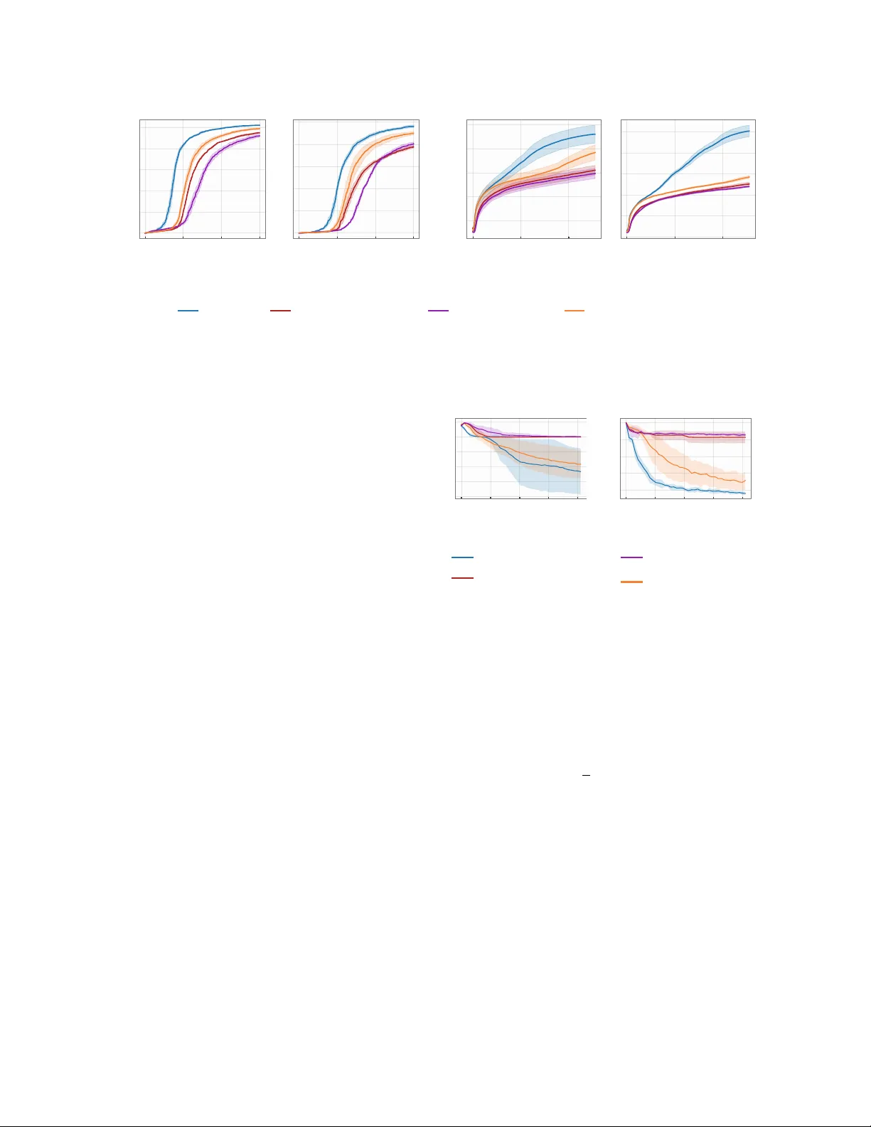
Generative Flow Networks (GFlowNets) are a flexible family of amortized samplers trained to generate discrete and compositional objects with probability proportional to a reward function. However, learning efficiency is constrained by the model's abi…
Authors: Pedro Dall'Antonia, Tiago da Silva, Daniel Csillag
Av oid What Y ou Kno w: Div ergen t T ra jectory Balance for GFlo wNets P edro Dall’An tonia 1 , Tiago da Silv a 2 , Daniel Csillag 1 , Salem Lahlou 2 , and Diego Mesquita 1 1 Sc ho ol of Applied Mathmatics, Getulio V argas F oundation 2 MBZUAI Abstract Generativ e Flo w Net works (GFlo wNets) are a flexible family of amortized samplers trained to generate discrete and compositional ob jects with probability proportional to a reward func- tion. Ho wev er, learning efficiency is constrained b y the mo del’s ability to rapidly explore di- v erse high-probabilit y regions during training. T o mitigate this issue, recent works hav e fo- cused on incentivizing the exploration of un- visited and v aluable states via curiosity-driv en searc h and self-supervised random net work distil- lation, which tend to w aste samples on already w ell-approximated regions of the state space. In this context, we prop ose A daptive Complemen- tary Explor ation (A CE), a principled algorithm for the effective exploration of no vel and high- probabilit y regions when learning GFlowNets. T o achiev e this, A CE introduces an explor ation GFlo wNet explicitly trained to search for high- rew ard states in regions underexplored by the c anonic al GFlowNet, whic h learns to sample from the target distribution. Through extensive exp er- imen ts, w e sho w that ACE significan tly improv es up on prior work in terms of appro ximation accu- racy to the target distribution and discov ery rate of diverse high-reward states. 1 In tro duction Generativ e Flow Net works [GFlo wNets; Bengio et al. , 2021 ] are p o werful reward-driv en genera- tiv e mo dels designed to sample from distributions o ver compositional ob jects (e.g., graphs and sequences), with a range of applications in scien- tific discov ery W ang et al. [ 2023 ], combinatorial optimization Zhang et al. [ 2023a , b ], and appro x- imate inference Malkin et al. [ 2023 ]. Building on the comp ositional structure of the target distribution’s supp ort, GFlo wNets create v alid samples by starting from an initial state and iter- ativ ely drawing from a forw ard p olicy . Learning a GFlowNet then b oils do wn to finding p olicies that satisfy a set of iden tities called b alanc e c onditions , which ensure sampling correctness. T o achiev e this, we train GFlo wNets by mini- mizing the logarithmic residuals of a balance con- dition ov er the state graph Malkin et al. [ 2022 ], Tiapkin et al. [ 2024 ]. Nonetheless, since analyt- ically sw eeping through the entire state graph is in tractable, w e instead av erage ov er the residuals in a set of sampled tra jectories. Conv en tionally , these tra jectories are drawn from an ϵ -greedy ex- plor atory p olicy consisting of a mixture of the forw ard and an uniform p olicy at each time step Bengio et al. [ 2023 ]. In theory , the uniform com- p onen t pro vides full supp ort to the sampling dis- tribution, prev enting mo de collapse. In practice, ho wev er, uniform search migh t not b e enough to warran t the exploration of m ultiple high- probabilit y regions if the target reward is sparsely distributed [ Malkin et al. , 2023 , Shen et al. , 2023 ]. T o impro ve exploration and provide b etter sup- p ort co verage, recent w orks considered learning the exploratory p olicy alongside the GFlowNet. Inspired b y curiosit y-driv en exploration, Kim et al. [ 2025a ] recen tly suggested training such a p olicy to sample from a log-linear mixture of the GFlo wNet’s loss and the reward function. Con- 1 T arget distrib ution Epochs 0 . 5 1 . 0 T otal variation ACE IR Forward Polic y Exploratory Policy A CE ( ours ) Intrinsic Rewards (IR) [Madan et al., 2025] Training Flo w Figure 1: When learning the exploratory p olicy based on a combination of intrinsic and extrinsic rew ards—see Equations ( 6 ) and ( 7 )—, the mo del ma y ov eremphasize well-learned states (b ottom ro w). In contrast, ACE avoids sampling tra jectories from ov er-explored regions of the state space by design (top row), whic h improv es mo de discov ery and accelerates learning conv ergence (rightmost panel) to the target. This figure shows the marginal distribution of forward and exploratory p olicies at different training p oin ts (marked as dashed vertical lines). curren tly , Madan et al. [ 2025 ] prop osed instead targeting a combination of the original (extrin- sic) reward and an intrinsic rew ard based on self- sup ervised random net work distillation (RND). In b oth cases, exploration is guided by a GFlo wNet steered by the loss function of an external deep neural net work—either that of the underlying sampler Kim et al. [ 2025a ], Malek et al. [ 2026 ] or the RND loss Madan et al. [ 2025 ]. T o distinguish the learned exploratory p olicy from the GFlowNet trained to sample from the target distribution, w e will refer to the latter as the c anonic al GFlo wNet. F rom a fundamental viewp oin t, the crux of designing an appropriate exploratory p olicy is ensuring it samples tra jectories from high-rew ard but underexplored regions during training. In this work, w e cast this problem as satisfying a new balance condition for exploration, which w e call diver gent tr aje ctory b alanc e (DTB). In a n utshell, DTB enforces standard tra jectory balance on under-sampled regions while imp osing zero probability to tra jectories terminating in o ver-sampled states. As a consequence, an y exploratory p olicy satisfying DTB concentrates its sampling on high-rew ard terminal states under-represen ted by the canonical GFlowNet. The ensuing algorithm, called A daptive Complementary Explor ation (A CE), can b e in terpreted as a t wo-pla y er game: the exploratory p olicy is contin ually adjusted to sample from under-sampled areas, and the GFlowNet b eing trained is up dated using tra jectories generated b y the exploratory p olicy and its own p olicy . In doing so, w e preven t the canonical GFlowNet from rep eatedly visiting only a small num b er of high-reward subsets of the state space, while ignoring others, a b eha vior known to slo w down training V emgal et al. [ 2023 ], Atanac ko vic and Bengio [ 2024 ]. W e also characterize the system’s equilibrium in Prop ositions 3.4 and 3.9 . When view ed through the lens of the flow net- w ork analogy , which inspired the developmen t of GFlo wNets Bengio et al. [ 2021 ], A CE implements a principled mechanism for transferring excess probabilit y mass from o ver- to under-allocated mo des. W e illustrate this in the diagram of Figure 1 . Our exp erimen ts on p eptide discov ery , bit sequence design, combinatorial optimization, and more, confirm ACE significantly speeds up training con v ergence and the disco v ery of div erse, high-rew ard states when compared against prior tec hniques for improv ed GFlowNet exploration. Our contributions are the following. 1. W e prop ose A daptive Complementary Ex- plor ation (A CE), a new metho d for effective state space exploration in GFlowNet training. Based on the nov el diver gent tr aje ctory b alanc e (DTB), ACE fo cuses on generating tra jectories from high-reward underexplored regions by the canonical GFlowNet, increas- 2 ing sample diversit y and mitigating mass concen tration on a few mo des. 2. W e sho w ACE prev en ts distributional collapse of the canonical GFlo wNet (Prop osition 3.8 ) b y biasing sampling tow ards infrequen tly visited but v aluable regions of the state space (Prop ositions 3.4 and 3.9 ). 3. W e ev aluate our metho d on diverse and stan- dard benchmark tasks, including the grid w orld, p eptide disco very , and bit sequence gen- eration, and sho w that it often results in dras- tically faster iden tification of div erse and high- rew ard states relatively to prior approaches. 2 Preliminaries and Related W orks Definitions. Our ob jective is to sample ob jects x from a discrete space X in prop ortion to a r ewar d function R : X → R + . W e sa y X is c omp ositional if there is a directed acyclic graph G = ( S ∪ X , E ) ov er an extension S ∪ X of X with edges E having the following prop erties. 1. There exists a unique s o ∈ S s.t. (i) s o is connected to any s ∈ S via a directed path, denoted s o ⇝ s , and (ii) s o has no incoming edges. W e call s o the initial state . 2. There exists a unique s f ∈ S s.t. (i) s → s f ∈ E if and only if s ∈ X and (ii) s f has no outgoing edges. W e refer s f as the final state and to X as the set of terminal states . Under these conditions, we refer to G as a state gr aph . Illustratively , let X b e the space of k -sized m ultisets with elements selected from { 1 , . . . , n } . Then, we construct G b y defining s o = ∅ and S as the space of m ultisets with size up to k − 1, includ- ing a directed edge from s to s ′ if and only if s ′ dif- fers from s b y a single additional element. Imp or- tan tly , although |X | = O ( n k ) is combinatorially explosiv e, each s ∈ S has exactly n c hildren in G . A GFlowNet is an amortized sampler defined o ver G . Section 2.1 reviews the formalism b ehind GFlo wNets, and Section 2.2 discusses the limitations of prior art addressing the problem of inefficient exploration in GFlowNet training. 2.1 GFlo wNets T o start with, w e recast the problem of directly sampling from R on X to that of learning an amortize d p olicy function p F : S × ( S ∪ X ) → [0 , 1] such that p F ( s, · ) is a probabilit y measure supp orted on the children of s in G . T o achiev e this goal, w e parameterize p F ( s, · ) as a softmax deep neural netw ork trained to satisfy p ⊤ ( x ) : = X τ : s o ⇝ x Y ( s,s ′ ) ∈ τ p F ( s, s ′ ) ∝ R ( x ) , (1) in whic h the sum co v ers all tra jectories from s o to x in G . W e refer to p F as the forwar d p olicy and p ⊤ ( · ) as its induced marginal distribution o ver X . F or conciseness, we will often omit s o and write p F ( τ ) : = Q ( s,s ′ ) ∈ τ p F ( s, s ′ ) as the forward probabilit y of a tra jectory τ in G . As exact computation of p ⊤ is in tractable, we introduce a b ackwar d p olicy p B : ( S ∪ X ) × S → [0 , 1] on the transp osed state graph G ⊺ , and join tly search for p F and p B satisfying the tr aje ctory b alanc e (TB) condition for a learned constant Z , Z · p F ( τ ) = p B ( τ | x ) · R ( x ) , (2) in which p B ( τ | x ) = Q ( s,s ′ ) ∈ τ p B ( s ′ , s ) is the bac kward probability of τ . As shown by Malkin et al. [ 2022 ], Madan et al. [ 2022 ], this can b e ac hieved b y solving the follo wing sto c hastic program ov er Z and p olicies p F and p B , min Z,p F ,p B E τ ∼ p E " log Z · p F ( τ ) p B ( τ | x ) R ( x ) 2 # , (3) in which p E is an explor atory p olicy fully supp orted on the tra jectories in G . Other loss functions, e.g., sub-tra jectory balance Madan et al. [ 2022 ] and detailed balance Bengio et al. [ 2023 ], hav e also b een studied. W e refer the reader to Viviano et al. [ 2025 ] for a mo dular implemen tation of these ob jectiv es and standard b enc hmarks. By letting θ b e the parameters of our mo dels for p F , p B and Z θ , we define L TB ( θ ; τ ) = log Z θ · p F ( τ ; θ ) p B ( τ | x ; θ ) R ( x ) 2 (4) If con text is clear, we will often exclude θ from the notations of p F and p B to av oid notational 3 0 25 50 75 0M 1M 2M 3M 4M Sampled trajectories 0 50 100 150 A CE ( Ours ) T rajectory Balance (Malkin et al., NeurIPS 2022) Figure 2: A GFlowNet trained on the Rings distribution (left) via ϵ -greedy exploration may o verdra w samples from a w ell-approximated region (p olygon), misrepresenting other high- probabilit y regions. The TB residual on the righ tmost panel for the inner (top) and outer (b ottom) rings shows A CE av oids this issue. clutter. Also, notice that a GFlowNet induces a reward function s.t., for each x ∈ X , ˆ R θ ( x ) = Z θ · p ⊤ ( x ) = E τ ∼ p B ( ·| x ) Z θ · p F ( τ ; θ ) p B ( τ | x ; θ ) . (5) In particular, when L TB ( θ ; τ ) = 0 for all τ , the induced rew ard ˆ R θ ( x ) matc hes the true reward R ( x ) for eac h x ∈ X . 2.2 Learning GFlowNets The choice of p E is paramount for the effective training of GFlowNets Bengio et al. [ 2021 ], Kim et al. [ 2025b ]. T raditionally , p E is defined as an ϵ -gr e e dy version of p F , p E ( s, · ) = (1 − ϵ ) p F ( s, · ) + ϵp U ( s, · ), in which p U ( s, · ) is an uniform distri- bution ov er the children of s in the state graph. F or multi-modal target distributions, how ev er, an ϵ -greedy p olicy might struggle to visit certain mo des when p F is near-collapsed into a subset of the high-probability regions, as b oth p U and p F w ould then assign negligible probability to the un- visited high-rew ard states during training. W e il- lustrate this phenomenon in Figure 2 . T o address this limitation, recent researc h has focused on the design of sophisticated metaheuristics Kim et al. [ 2024 ], Boussif et al. [ 2024 ], reward shaping Pan et al. [ 2023 ], Jang et al. [ 2024 ], and ad ho c tec h- niques Rector-Bro oks et al. [ 2023 ], Hu et al. [ 2025 ] for enhanced state graph exploration, which can b e used complementarily to our metho d. Additionally , there is a growing b o dy of literature show casing the effectiv eness of param- eterizing p E as an explor ation GFlowNet trained to sample from a nov elt y-promoting mo dification of R . Inspired by the literature of curiosit y- driv en learning, for instance, Kim et al. [ 2025a ] suggested training p E to sample from a w eighted a verage b et ween R ( x ) and the loss function L TB in Equation ( 4 ) in log-space, that is, log R A T ( x ) = log R T ( x ) + α log R ( x ) , with α > 0 and, defining δ ( τ ) : = log R ( x ) + log p B ( τ | x ) − log p F ( τ ) − log Z as the base residual in Equation ( 3 ), and the teac hers log reward, log R T ( x ), as E τ ∼ p B ( ·| x ) log ϵ + 1 + C · 1 δ ( τ ) > 0 δ ( τ ) 2 . (6) W e refer to this class of metho ds as Adaptive T eac hers (A T) GFlo wNets throughout this w ork. Similarly , Madan et al. [ 2025 ] prop osed in tro ducing intrinsic r ewar ds based on random net work distillation [RND; Burda et al. , 2018 ] as a pro xy for nov elt y when learning p E , resulting in R SA ( x ; τ ) = R ( x ) β 1 + X s ∈ τ R A ( s ) ! β 2 β 3 , (7) in which β 1 , β 2 , β 3 > 0 are p ositiv e constan ts and R A ( s ) = ∥ ψ ( s ) − ψ random ( s ) ∥ 2 is based on RND of a neural net work ψ in to a randomly fixed mo del ψ random P an et al. [ 2023 ]. The reader should no- tice that the reward function R SA for p E is path- dep enden t. As in Madan et al. [ 2025 ], we call this approac h Sibling Augmented (SA) GFlowNets. F rom an empirical standp oin t, how ever, R T and R A are incomparable to R . The reason for this is that while R often represents a ph ysical quan tity , suc h as binding affinity of drugs Bengio et al. [ 2021 ] or a Ba yesian p osterior Malkin et al. [ 2023 ], R T and R A are simply error functions of neural netw orks designed to capture no velt y indir e ctly . Hence, the mechanisms b y 4 whic h either metho d addresses the problem of insufficien t exploration of high-rew ard regions that hamp ers GFlowNet training remain elusive. W e defer a comprehensive discussion of related w orks to Section B in the supplement. Our method, presented in the next section, circum ven ts this issue by dir e ctly promoting the visitation of nov el states through the nov el diver gent tr aje ctory b alanc e (DTB) loss. 3 Adaptiv e Complemen tary Exploration Div ergent T ra jectory Balance. During training, the canonical GFlowNet may o ver- allo cate probability mass to certain tra jectories, hamp ering exploration of no vel and high-reward regions. W e illustrate this in Figure 2 . When trained to sample from the Rings distribution (see Section 4 ) via ϵ -greedy exploration, a GFlo wNet concentrates most of its probabilit y in a single high-reward region of the state space, under-represen ting the second, more distant mo de. T o formalize this intuition, we define the set of o v er-sampled tra jectories below. F or clarit y , w e will refer to a GFlowNet as g = ( Z, p F , p B ). Definition 3.1 (Over- & Under-Allo cated re- gions) . Let g = ( Z, p F , p B ) b e a GFlo wNet and α > 0. W e define the set of over-al lo c ate d states with resp ect to α as O A( α, g ) = { x ∈ X : ˆ R g ( x ) ≥ α · R ( x ) } , in which ˆ R g is the GFlo wNet’s induced reward function describ ed in Equation ( 5 ). Similarly , w e define the set of state s with under-al lo c ate d probabilit y mass as UA( α, g ) = X \ O A( α, g ) With a slight abuse of notation, we write τ ∈ OA ( α, g ) (resp. τ ∈ UA ( α, g )) to indi- cate that τ starts at s o and finishes at some x ∈ OA ( α, g ) (resp. x ∈ UA ( α, g )). When g is clear, we will simply write OA( α ) and UA( α ). Our ob jective is to learn an exploratory p olicy sampling high-reward states in UA ( α ) while a voiding tra jectories in O A ( α ). This can b e ac hieved by enforcing the DTB condition (Def- inition 3.2 ). Given the terminology , we denote the exploration GFlowNet as g ∇ = ( Z ∇ , p ∇ F , p ∇ B ). Definition 3.2 (DTB) . Let g and g ∇ b e GFlo wNets. W e define the diver gent tr aje ctory b alanc e (DTB) of g ∇ with r esp e ct to g for a threshold α > 0 and exp onen t β > 0 as Z ∇ · p ∇ F ( τ ) = R ( x ) β · p ∇ B ( τ | x ) if τ ∈ UA( α, g ) , Z ∇ · p ∇ F ( τ ) = 0 otherwise. As in Definition 3.1 , we will often omit α , β , and g when referring to the DTB of g ∇ . Similarly to prior w ork Madan et al. [ 2025 ], Kim et al. [ 2025a ], w e train the exploration GFlo wNet on a temp ered rew ard function to facilitate state space na vigation, a technique that has b een empirically sho wn to b e effective Zhou et al. [ 2023 ] and is ro oted in the literature of sim ulated annealing for Marko v chain Mon te Carlo Kirkpatrick et al. [ 1983 ]. In tuitively , the DTB prunes the supp ort of p ∇ F to the set of tra jectories with under-allo cated probabilit y mass by the canonical GFlo wNet ( g ). The v alue of α dictates ho w muc h of p ∇ F ’s supp ort is trimmed, with larger v alues corresp onding to larger supp orts (i.e., α 7→ UA( α ) is increasing w.r.t. set inclusion). In order to learn an exploration GFlowNet g ∇ abiding by the conditions in Definition 3.2 , w e design a loss function we can optimize via gradien t descent. T ow ards this goal, we notice that the DTB conditions can b e rewritten as Z ∇ ϕ p ∇ F ( τ ; ϕ ) = R ( x ) p ∇ B ( τ ; ϕ ) I [ τ ∈ UA( α, g )] , ∀ τ ; equiv alen tly , dividing by R ( x ) p ∇ B ( τ ; ϕ ) and adding I [ τ ∈ O A ( α, g )] on b oth sides (recall that O A( α ) ∪ UA( α ) : = X ), Z ∇ ϕ p ∇ F ( τ ; ϕ ) R ( x ) p ∇ B ( τ ; ϕ ) + I [ τ ∈ O A( α, g )] = 1 , ∀ τ . (8) Dra wing on this, we define the diver gent tr aje c- tory b alanc e loss L ∇ as the log-squared residual b et w een the left- and right-hand sides of Equa- tion ( 8 )—analogously to the TB Malkin et al. [ 2022 ] and SubTB Madan et al. [ 2022 ] losses. 5 Definition 3.3 (DTB Loss) . Let g and g ∇ b e GFlo wNets. W e define the DTB loss L ∇ ( g ∇ ; τ , α ) of the exploration GFlowNet g ∇ for a tra jectory τ and threshold α > 0 as log Z ∇ ϕ p ∇ F ( τ ; ϕ ) R ( x ) β p ∇ B ( τ ; ϕ ) + I [ τ ∈ O A( α )] ! 2 . (9) W e also define L ∇ ( g ∇ ; g , α ) = E τ ∼ p ϵ, ∇ F [ L ∇ ( g ∇ ; τ , α )] as the av erage of L ∇ with resp ect to the ϵ -greedy v ersion p ϵ, ∇ F of p ∇ F , wherein w e make the dep endence of L ∇ on the canonical GFlo wNet g (via the set OA) explicit. When optimized to zero, L ∇ driv es the exploratory p olicy p ∇ F to sample prop ortionally to the reward in undersampled areas (i.e., UA( α )). W e formalize this in Prop osition 3.4 . Prop osition 3.4 (Complemen tary Sampling Prop ert y) . Assume L ∇ ( g ∇ ; τ , α ) = 0 for e ach tr aje ctory τ starting at s o and finishing at a terminal state in X and UA ( α ) = ∅ . Then, the mar ginal p ∇ ⊤ of p ∇ F over X is p ∇ ⊤ ( x ) ∝ R ( x ) β · I [ x ∈ UA( α )] , with normalizing c onstant Z ∇ = P x ∈ UA( α ) R ( x ) β . F rom an information-theoretic p ersp ectiv e, minimizing the exp ectation of L ∇ under a mea- sure µ supp orted on tra jectories in O A ( α ) may b e in terpreted as maximizing a Kullbac k-Leibler di- v ergence Kullback and Leibler [ 1951 ] based on µ . Prop osition 3.5 (Repulsive Bound) . L et µ b e a pr ob ability me asur e over tr aje ctories supp orte d on O A ( α ) , and define p ∇ B ( τ ) = π ( x ) p ∇ B ( τ | x ) as the b ackwar d tr aje ctory pr ob ability, with π ( x ) ∝ R ( x ) as the normalize d tar get. Then, E τ ∼ µ " log p ∇ F ( τ ) p ∇ B ( τ ) + I [ τ ∈ O A( α )] 2 # ≥ log(2) + D K L [ µ ∥ p ∇ B ] − D K L [ µ ∥ p ∇ M ] 2 , (10) in which p ∇ M = 1 2 ( p ∇ F + p ∇ B ) . This quantity is minimize d when the mar ginal distribution p ∇ ⊤ of p ∇ F on X vanishes on O A( α ) . Algorithm 1 Adaptive Complemen tary Explo- ration (ACE) Require: Rew ard function R ( x ), threshold α 1: GFlo wNets g ← ( θ, Z θ ) and g ∇ ← ( ϕ, Z ∇ ϕ ) 2: while not con verged do 3: // Phase 1: Sampling 4: B ← { τ ∼ p F ( · ; θ ) } 5: B ∇ ← { τ ∼ p ϵ, ∇ F ( · ; ϕ ) } 6: // Phase 2: Exploitation Up date 7: Calculate mixing weigh t: 8: w ← sg Z θ Z θ + Z ϕ 9: L 1 ← 1 |B| P τ ∈B L TB ( θ ; τ ) 10: L 2 ← 1 |B ∇ | P τ ∈B ∇ L TB ( θ ; τ ) 11: L ← w · L 1 + (1 − w ) L 2 12: Up date θ b y a gradient step on ∇ θ L . 13: // Phase 3: Exploration Up date 14: L exp ← 1 |B ∇ | P τ ∈B ∇ L ∇ ( ϕ ; τ , α ) 15: Up date ϕ by a gradient step on ∇ ϕ L exp . 16: end while Adaptiv e Complemen tary Exploration. As men tioned earlier, w e train the canonical GFlo wNet g on samples from b oth g and g ∇ b y generating tra jectories from the mixture p ACE F ( s o , · ) = w · p F ( s o , · ) + (1 − w ) · p ϵ, ∇ F ( s o , · ) . (11) This raises the question: how to choose w to b et- ter emphasize diverse high-reward states during training? In tuitively , w e would lik e w → 1 as the canonical GFlowNet g co vers a progressively large p ortion of the high-probabilit y regions in the state space, and that w < 0 . 5 when g ∇ concen trates most of the probability mass in X . By construc- tion, under the ligh t of Bengio et al. [ 2023 , Prop o- sition 10] and Prop osition 3.4 , we notice that the learned Z and Z ∇ serv e as proxies for the rew ard masses under g and g ∇ , resp ectively . With this in mind, we define w as the r elative mass under g , w = Z Z ∇ + Z . As we will sho w in Prop osition 3.9 , such a choice satisfies the desiderata ab o v e. Based on this, w e define the loss function for the canonical GFlo wNet b elo w. 6 0 128000 256000 Trajectories 0 . 0 0 . 5 1 . 0 1 . 5 2 . 0 T op-200 Reward × 10 13 K = 24 0 128000 256000 Trajectories 0 . 0 0 . 5 1 . 0 1 . 5 2 . 0 × 10 18 K = 32 (a) Sequence design. 0 64000 128000 192000 Trajectories 0 . 0 0 . 5 1 . 0 1 . 5 2 . 0 2 . 5 T op-200 Reward × 10 8 K = 32 0 64000 128000 192000 Trajectories 0 . 0 0 . 2 0 . 4 0 . 6 0 . 8 1 . 0 × 10 8 K = 64 (b) Bit sequences. A CE ( Ours ) Trajectory Balance [Malkin et al., NeurIPS 2022] Adaptiv e T eacher [Kim et al., ICLR 2025] Sibling Augmented [Madan et al., ICLR 2025] Figure 3: A CE significantly accelerates mo de-disco very for autoregressive sequence generation with GFlowNets. Eac h plot shows the a verage reward of the unique 200 highest-v alued disco vered states as a function of the num b er of tra jectories sampled throughout training. Definition 3.6 (Canonical Loss ) . Let g and g ∇ b e the canonical and exploration GFlowNets. W e define the c anonic al loss as the tra jectory balance loss a veraged ov er the mixture distribution p ACE F in Equation ( 11 ), i.e., L CAN ( g ; g ∇ ) = sg( w ) · E τ ∼ p F [ L TB ( g ; τ , R )] + sg (1 − w ) · E τ ∼ p ϵ, ∇ F [ L TB ( g ; τ , R )] , (12) with sg as the stop-gradien t op eration, e.g., jax.stop gradient in JAX Bradbury et al. [ 2018 ] or torch.Tensor.detach in PyT orc h P aszke et al. [ 2019 ], which detac hs w from the computation graph. W e call A daptive Complementary Explor ation (A CE) the algorithm that learns b oth g and g ∇ b y minimizing the Canonical (Definition 3.6 ) and DTB (Definition 3.3 ) losses via Mon te Carlo estimators based on their resp ectiv e integrating measures. W e summarize ACE in Algorithm 1 . There, to determine whether τ ∈ OA ( α ) in Equation ( 9 ), w e use a single monte carlo sample from p B ( ·| x ) to estimate ˆ R g ( x ). R emark 3.7 (Notation for the loss functions) . T o emphasize the parameterization of our mo dels, w e also denote by L TB ( θ ; τ ) and L ∇ ( ϕ ; τ , α ) the losses ev aluated at τ for GFlowNets g and g ∇ with parameters θ and ϕ , resp ectiv ely . Notably , when g and g ∇ collapse in to a subset of X , the exp ected on-policy gradient of L ∇ pushes g ∇ to wards the complement of that subset; see Prop osition 3.8 . Recall that we up date ϕ via gradien t steps in the direction of −∇ ϕ L ∇ . Prop osition 3.8. Assume g and g ∇ ar e c ol lapse d on a set C ⊂ X , i.e., p ⊤ (C) = 1 and p ∇ ⊤ (C) = 1 , that they satisfy their r esp e ctive TB c onditions on al l tr aje ctories le ading to C , and α < 1 . Then, if g ∇ is p ar ameterize d by ϕ = ( ϕ F , ϕ B , Z ∇ ) , ϕ F and ϕ B as the p ar ameters for p ∇ F and p ∇ B , E τ ∼ p ∇ F ( · ; ϕ F ) ∇ ϕ F L ∇ ( ϕ ; τ , α ) = − log (2) ∇ ϕ F p ∇ ⊤ (C c ; ϕ F ) , in which p ∇ ⊤ is as in Equation ( 1 ) and C c : = X \ C . W e also demonstrate that the equilibrium of the co op erativ e game implemented by Algorithm 1 dep ends on the choice of α . Prop osition 3.9 (Equilibrium State) . Assume g ⋆ = ( Z ⋆ , p ⋆ F , p ⋆ B ) and g ⋆ ∇ = ( Z ⋆ ∇ , p ∇ ,⋆ F , p ∇ ,⋆ B ) jointly satisfy g ⋆ = arg min g L CAN ( g ; g ⋆ ∇ ) and g ⋆ ∇ = arg min g ∇ L ∇ ( g ∇ ; g ⋆ , α ) . Then, Z ⋆ : = P x ∈X R ( x ) and p ⋆ ⊤ ( x ) ∝ R ( x ) . When α ≤ 1 , Z ⋆ ∇ = 0 . When α > 1 , Z ⋆ ∇ = P x ∈X R ( x ) β and p ∇ ,⋆ ⊤ ( x ) ∝ R ( x ) β , in which p ∇ ,⋆ ⊤ is the mar ginal distribution over X induc e d by g ⋆ ∇ (r e c al l Equation 1 ). 7 0 16000 32000 48000 Trajectories 0 100 200 300 400 500 T op-200 Reward K = 18 0 16000 32000 48000 Trajectories 0 100 200 300 400 500 K = 24 (a) Bag generation. 0 3200 6400 Trajectories 10 15 20 25 30 T op-200 Reward K = 128 0 3200 6400 Trajectories 10 20 30 40 50 60 K = 256 (b) Quadratic knapsack. A CE ( Ours ) Trajectory Balance [Malkin et al., NeurIPS 2022] Adaptiv e T eacher [Kim et al., ICLR 2025] Sibling Augmented [Madan et al., ICLR 2025] Figure 4: ACE finds diverse and high-rew ard states faster than prior approaches for impro ved GFlo wNet exploration for the bag generation (left) and quadratic knapsack (righ t) problems. In b oth (a) and (b), K denotes the n umber of av ailable items for selection. If α ≤ 1, for instance, the repulsiv e force de- scrib ed in Prop osition 3.5 forces g ∇ to collapse in to Z ∇ = 0. Oh terwise, if α > 1, the exploration GFlo wNet matches the temp ered target R ( x ) β . T ogether, these results establish ACE as a principled approach for enhanced exploration of rew ard-dense regions during GFlowNet training. Imp ortan tly , the next section shows that A CE also consisten tly outp erforms prior art on stan- dard metrics used in the GFlowNet literature. 4 Exp erimen ts W e present a comprehensive empirical analysis of our metho d in this section. The central research questions (RQs) our campaign aims to resp ond are the following. R Q1 Do es ACE significan tly sp eed up the num- b er of div erse and high-reward states found during learning? R Q2 Do es ACE accelerate learning conv er- gence? W e answer b oth in the affirmativ e by measuring the top- K a verage reward of unique states found throughout training Pan et al. [ 2023 ], Madan et al. [ 2022 , 2025 ], the conv ergence rate of the log-partition function of the canonical GFlowNet, and the total v ariation (TV) distance b etw een 0M 1M 2M 3M 4M Sampled trajectories 0 .2 .4 .6 .8 1 TV distance (a) Rings . 0M 1M 2M 3M 4M Sampled trajectories .2 .4 .6 .8 1 TV distance (b) 8 Ga ussians. A CE ( Ours ) Trajectory Balance [Malkin et al., NeurIPS 2022] Adaptiv e T eacher [Kim et al., ICLR 2025] Sibling Augmented [Madan et al., ICLR 2025] Figure 5: ACE results in faster learning con vergence than prior art for GFlo wNet exploration for the Lazy Random W alk task. Please consult Figure 6 b elo w for the legend. the learned and target distributions, defined as TV( p ⊤ , π ) : = 1 2 X x ∈X | p ⊤ ( x ) − π ( x ) | , in which π ( x ) ∝ R ( x ) is the normalized target and p ⊤ is the GFlowNet’s marginal ov er terminal states; see Equation ( 1 ). Collectiv ely , our exp erimen ts confirm that ACE is an effective algorithm that drastically improv es the sample efficiency of GFlowNets. W e refer the reader to Section C in the supplement for further details on our exp erimen ts. Lazy Random W alk. The state space S is [[ − m, m ]] d × { 1 , . . . , T − 1 } for m, d, T ∈ N with md ≤ T , and X : = [[ − m, m ]] d × { T } , and 8 [[ − m, m ]] = {− m, − m + 1 , . . . , m } . The initial state is s o = ( 0 d , 1) = ([0 , . . . , 0] , 1) and eac h tran- sition at ( s , t ) corresp onds to either adding 1 or − 1 to a chosen coordinate of s or sta ying in place; in either case, the coun ter t is incremen ted to t + 1. This is rep eated until t = T (full details in Sec- tion C). W e let α = 0 . 2. In particular, we assess A CE on b oth Rings —shown in Figure 2 —and 8 Gaussians distributions; Figure 5 highlights A CE achiev es the b est distributional fit. Grid world. Malkin et al. [ 2022 ], Madan et al. [ 2025 ] T o further gauge ACE, we consider the standard grid w orld environmen t. There, S = [[0 , H ]] d and X = S × {⊤} , in whic h ⊤ is an indicator of finalit y . The sampler starts at s o = 0 , and at each state s w e either add 1 to a co ordinate of s or transition to x : = s × {⊤} ∈ X . W e let H = 16, d = 2, y ( x ) = | 5 · x / H − 10 | , and train a GFlo wNet to sample from R ( x ) = 10 − 3 + 3 · Y 1 ≤ i ≤ d [ y ( x i ) ∈ (6 , 8)] (13) in which [ C ] represents Iverson’s brac ket, which ev aluates to 1 if the clause C is true and 0 otherwise; see Figure 1 . Differently from Lazy Random W alk, the stopping action poses additional exploration challenges, as a randomly initialized sampler is less likely to encounter the distan t (in Euclidean norm) modes from s o Shen et al. [ 2023 ]. Notably , Figure 6 shows that ACE results in faster training con vergence than b oth A T, SA, and ϵ -greedy GFlowNets. Bit sequences. Malkin et al. [ 2022 ], Madan et al. [ 2022 ] W e define S = S k ≤ K − 1 { 1 , 0 } k and X = { 1 , 0 } K for a given sequence size K . As in Malkin et al. [ 2022 ], we let M ⊆ X b e a set of mo des and log R ( x ) = 1 T (1 − min m ∈M d ( x,m ) / K ) , in whic h d ( x, m ) represen ts Lev enshtein’s distance b et w een binary strings x and m and T = 1 / 20 . Concretely , S represen ts the space of bit sequences with size up to K − 1. Starting at s o = [], we app end either 1 or 0 to the current state until it reaches the size of K . W e consider K ∈ { 32 , 64 } . Notably , Figure 3b shows that our metho d finds div erse high-reward states significan tly faster than baselines. Sequence design. Silv a et al. [ 2025 ] Similarly , S = S k ≤ K − 1 V k for a finite v o cabulary V 0 . 0 0 . 5 1 . 0 1 . 5 Sampled trajectories × 10 6 0 . 2 0 . 4 0 . 6 0 . 8 1 . 0 TV distance 0 . 0 0 . 5 1 . 0 1 . 5 Sampled trajectories × 10 6 0 2 4 6 8 log Z A CE ( Ours ) Trajectory Balance [Malkin et al., NeurIPS 2022] Adaptiv e T eacher [Kim et al., ICLR 2025] Sibling Augmented [Madan et al., ICLR 2025] Figure 6: ACE ac hiev es the b est go o dness- of-fit to the target distribution in the grid world task describ ed in Equation ( 13 ). and K , and X = V K with size V : = |V | . W e consider ( K, V ) ∈ { (24 , 6) , (32 , 4) } , and define the rew ard function of a x ∈ X through log R ( x ) : = P K k =1 u ( k ) · v ( x k ), in which u : [ K ] → R and v : V → R are utility functions pic ked at random prior to training. (Recall [ K ] = { 1 , . . . , K } ). Remark ably , Figure 3a confirms that A CE significantly increase the disco very rate of high-reward regions for this task. Bag generation. Shen et al. [ 2023 ], Jang et al. [ 2024 ] A bag is a multiset with elements taken from a set V . In Figure 4a , we let S : = { B ⊆ multi V : |B | < S } and X : = { B ⊆ multi V : |B | = S } b e the set of S -sized m ulti-subsets of a set V with size K , and define R ( x ) = P e ∈ x u ( e ) for an utilit y function u : V → R + dra wn from a geometric Gaussian pro cess. Once again, ACE improv es up on prior approaches in terms of the sp eed with whic h high-probability regions are discov ered. Quadratic Knapsac k. W e present results for the Quadratic Knapsack task, whic h is an NP-hard problem Caprara et al. [ 1999 ]. Briefly , w e let W b e the maximum weigh t, w ∈ R K + b e the weigh t of each of the K items, u ∈ R K + b e their utilities, and A ∈ R K × K b e a symmetric matrix measuring the substitutability or comple- men tarity of each item pair. W e may choose up to L copies of each item, and our ob jectiv e is to find the item multiplicities m = ( m 1 , . . . , m K ) maximizing the collection’s utility , i.e., max m ∈ [[0 ,L ]] K ⟨ u , m ⟩ + m ⊤ A m s.t. ⟨ m , w ⟩ ≤ W . (14) W e let K ∈ { 128 , 256 } and W = 60. Our 9 P1 P2 P3 P4 A CE (Ours) − 4 − 2 0 2 4 6 8 2 4 6 8 10 12 14 16 P1 P2 P3 P4 (Malkin et al., 2022) − 4 − 2 0 2 4 6 8 2 4 6 8 10 12 14 16 (Kim et al., 2025b) − 4 − 2 0 2 4 6 8 2 4 6 8 10 12 14 16 (Madan et al., 2025) − 4 − 2 0 2 4 6 8 2 4 6 8 10 12 14 16 Figure 7: Peptide embeddings colored b y predicted micro-organism group. Eac h dot represen ts the 2D pro jection of the k-mer embedding of the AMPs in Figure 8 . As we can see, A CE generates a substan tially more diverse set of AMPs with likely antimicrobial activity than alternativ e metho ds. W e show case a subset of ACE’s generated p eptides in in the leftmost panel. ACE ( Ours ) Trajectory Balance [Malkin et al., NeurIPS 2022] Adaptive T eacher [Kim et al., ICLR 2025] Sibling Augmented [Madan et al., ICLR 2025] Figure 8: ACE iden tifies a larger n umber of high-fitness AMPs than prior metho ds. The plot shows the num b er of unique AMPs found during training with at least 95% probabilit y of exhibiting an timicrobial activity as a function of the num b er of tra jectories. generativ e pro cess starts at s o = 0 ∈ R K , and at eac h step w e add an item to the curren t state s un til no items can b e added (either due to rep etition or weigh t limit). In this setting, S = { m ∈ [[0 , L ]] K : ∃ k , ⟨ m , w ⟩ + w k ≤ W and m k + 1 ≤ L } , and X is defined as the set for which such a k do es not exist, i.e., for which no more items can b e added to the collection. The rew ard function R b eing defined as the ob jective function in Equation ( 14 ). As previously noted, ACE exhibits the b est sample efficiency in the search for high-v alued feasible solutions for the Quadratic Knapsack problem. An timicrobial Peptides (AMPs). T rabucco et al. [ 2022 ], Jain et al. [ 2022 ] W e also ev aluate A CE on the task of de novo design of AMPs p oten tially active against the following pathogens: E. c oli , S. aur eus , P. aeruginosa , B. subtilis , and C. albic ans . The p eptide design space is restricted to sequences with up to 10 amino acids. Given the standard proteinogenomic alphab et, consisting of 20 standard amino acids, this results in a search space with 10 13 candidates. F ormally , the initial state is s o = [], the state space S consists of all amino acid sequences of size up to L = 10, and X = { s ⊕ ⟨ EOS ⟩ : s ∈ S } , in whic h ⟨ EOS ⟩ is a special end-of-sequence tok en and ⊕ represen ts the concatenation operator; for A CE, we let α = 0 . 2 and β = 1. The reward is de- riv ed from a Random F orest classifier P edregosa et al. [ 2011 ], Dall’Antonia et al. [ 2025 ] predicting an timicrobial activity across pathogens (full de- tails in Section C ); we use a cutoff c = 0 . 95 and call a sequence a mo de if its predicted activity probabilit y satisfies p ( s ) ≥ c . Crucially , Figure 8 shows that ACE discov ers substan tially more unique high-rew ard AMPs throughout training than all comp eting meth- o ds. On the log-scaled y -axis, ACE ac hieves an order-of-magnitude impro vemen t in the cum ulative num ber of unique effectiv e p eptides, indicating b oth faster mo de discov ery and sustained exploration. T o further assess diversit y , Figure 7 visualizes the modes found during training via a 2D UMAP pro jection of their k -mer frequency em b eddings, highlighting the significan tly broader cov erage achiev ed by ACE. 10 5 Discussion W e in tro duced A daptive Complementary Ex- plor ation (ACE) as a principled algorithm for effectiv e exploration of underexplored regions during the training of GFlowNets. While former approaches fo cused on learning an exploratory p olicy via curiosity-driv en metho ds, whic h we ha ve sho wn may o veremphasize w ell- appro ximated regions of the state space (e.g., Figure 1 ), ACE promotes the visitation of no vel states through the newly prop osed diver gent tr aje ctory b alanc e (DTB) loss. Imp ortan tly , w e pro ved that the minimization of DTB pushes the exploratory p olicy a wa y from ov ersampled tra- jectories by the canonical GFlowNet, providing a rigorous foundation for our metho d. Our exp eriments demonstrated ACE con- sisten tly and significantly outp erformed prior approac hes for improv ed GFlowNet exploration in terms of the discov ery rate of diverse, high-rew ard regions and the go odness-of-fit to the target distribution. In conclusion, w e also b eliev e that exploring whether a non-stationary rew ard (e.g., curiosit y-driven) can b e used in Definition 3.2 and how to optimally w eight the GFlo wNets’ samples in Equation ( 11 ) are promising directions for future research. References Emman uel Bengio, Moksh Jain, Maksym Ko- rably ov, Doina Precup, and Y oshua Bengio. Flo w netw ork based generative mo dels for non-iterativ e diverse candidate generation. In NeurIPS (NeurIPS) , 2021. Hanc hen W ang, Tianfan F u, Y uanqi Du, W enhao Gao, Kexin Huang, Ziming Liu, Pa yal Chan- dak, Shengc hao Liu, Peter V an Katwyk, An- dreea Deac, et al. Scientific discov ery in the age of artificial in telligence. Natur e , 620(7972): 47–60, 2023. Dingh uai Zhang, Hanjun Dai, Nikola y Malkin, Aaron Courville, Y oshua Bengio, and Ling Pan. Let the flo ws tell: Solving graph combinato- rial optimization problems with gflo wnets. In NeurIPS (NeurIPS) , 2023a. Da vid W Zhang, Corrado Rainone, Markus P eschl, and Rob erto Bondesan. Robust schedul- ing with gflo wnets. In International Confer enc e on L e arning R epr esentations (ICLR) , 2023b. Nik olay Malkin, Salem Lahlou, T ristan Deleu, Xu Ji, Edw ard Hu, Katie Everett, Dinghuai Zhang, and Y oshua Bengio. GFlo wNets and v ariational inference. International Confer enc e on L e arning R epr esentations (ICLR) , 2023. Nik olay Malkin, Moksh Jain, Emman uel Ben- gio, Chen Sun, and Y oshua Bengio. T ra jec- tory balance: Impro ved credit assignment in GFlo wnets. In NeurIPS (NeurIPS) , 2022. Daniil Tiapkin, Nikita Morozov, Alexey Naumov, and Dmitry V etrov. Generative flow net works as entrop y-regularized rl, 2024. Y osh ua Bengio, Salem Lahlou, T ristan Deleu, Edw ard J. Hu, Mo Tiwari, and Emmanuel Bengio. Gflownet foundations. Journal of Machine L e arning R ese ar ch (JMLR) , 2023. Max W. Shen, Emmanuel Bengio, Ehsan Ha ji- ramezanali, Andreas Louk as, Kyunghyun Cho, and T ommaso Biancalani. T ow ards understand- ing and improving gflownet training. In In- ternational Confer enc e on Machine L e arning , 2023. Minsu Kim, Sanghy eok Choi, T aeyoung Y un, Emman uel Bengio, Leo F eng, Jarrid Rector- Bro oks, Sungso o Ahn, Jinkyoo Park, Nik olay Malkin, and Y osh ua Bengio. Adaptiv e teachers for amortized samplers. International Con- fer enc e on L e arning R epr esentations (ICLR) , 2025a. Kanik a Madan, Alex Lamb, Emman uel Bengio, Glen Berseth, and Y oshua Bengio. T ow ards im- pro ving exploration through sibling augmented gflo wnets. In International Confer enc e on R epr esentation L e arning (ICLR) , pages 89636– 89654, 2025. 11 Idriss Malek, Aya Laa jil, Abhijith Sharma, Eric Moulines, and Salem Lahlou. Loss-guided aux- iliary agents for ov ercoming mo de collapse in gflo wnets, 2026. URL abs/2505.15251 . Nikhil V emgal, Elaine Lau, and Doina Precup. An empirical study of the effectiv eness of using a replay buffer on mo de disco very in gflownets, 2023. URL 07674 . Lazar A tanack o vic and Emmanuel Bengio. In- v estigating generalization b eha viours of gen- erativ e flow netw orks, 2024. URL https: //arxiv.org/abs/2402.05309 . Kanik a Madan, Jarrid Rector-Bro oks, Maksym Korably ov, Emman uel Bengio, Moksh Jain, Andrei Cristian Nica, T om Bosc, Y osh ua Ben- gio, and Nik olay Malkin. Learning gflownets from partial episo des for improv ed conv ergence and stability . In International Confer enc e on Machine L e arning , 2022. Joseph D. Viviano, Omar G. Y ounis, Sanghy eok Choi, Victor Schmidt, Y osh ua Bengio, and Salem Lahlou. torchgfn: A pytorc h gflo wnet library , 2025. URL 2305.14594 . Hy eonah Kim, Minsu Kim, T aey oung Y un, Sangh yeok Choi, Emmanuel Bengio, Alex Hern´ andez-Garc ´ ıa, and Jinky o o Park. Im- pro ved off-p olicy reinforcement learning in bi- ological sequence design, 2025b. URL https: //arxiv.org/abs/2410.04461 . Minsu Kim, T aey oung Y un, Emmanuel Bengio, Dingh uai Zhang, Y osh ua Bengio, Sungso o Ahn, and Jinkyoo P ark. Lo cal searc h gflo wnets, 2024. URL . Oussama Boussif, L ´ ena N ´ ehale Ezzine, Joseph D Viviano, Micha l Koziarski, Moksh Jain, Nik o- la y Malkin, Emmanuel Bengio, Rim Assouel, and Y oshua Bengio. Action abstractions for amortized sampling, 2024. URL https:// arxiv.org/abs/2410.15184 . Ling P an, Nikola y Malkin, Dinghuai Zhang, and Y osh ua Bengio. Better training of GFlowNets with lo cal credit and incomplete tra jectories. In International Confer enc e on Machine L e arning (ICML) , 2023. Hy oso on Jang, Minsu Kim, and Sungso o Ahn. Learning energy decomp ositions for partial in- ference in GFlo wnets. In The Twelfth Interna- tional Confer enc e on L e arning R epr esentations , 2024. Jarrid Rector-Brooks, Kanik a Madan, Moksh Jain, Maksym Korablyo v, Cheng-Hao Liu, Sarath Chandar, Nikola y Malkin, and Y oshua Bengio. Thompson sampling for improv ed ex- ploration in gflownets, 2023. Rui Hu, Yifan Zhang, Zhuoran Li, and Longb o Huang. Beyond squared error: Exploring loss design for enhanced training of genera- tiv e flow netw orks. In The Thirte enth Interna- tional Confer enc e on L e arning R epr esentations , 2025. URL https://openreview.net/forum? id=4NTrco82W0 . Y uri Burda, Harrison Edwards, Amos Storkey , and Oleg Klimo v. Exploration b y random net- w ork distillation, 2018. URL https://arxiv. org/abs/1810.12894 . Mingy ang Zhou, Zichao Y an, Elliot Layne, Nik o- la y Malkin, Dinghuai Zhang, Moksh Jain, Mathieu Blanc hette, and Y oshua Bengio. Phy- logfn: Phylogenetic inference with generative flo w netw orks, 2023. Scott Kirkpatrick, C Daniel Gelatt Jr, and Mario P V ecc hi. Optimization by simulated annealing. scienc e , 220(4598), 1983. S. Kullback and R. A. Leibler. On Information and Sufficiency. The A nnals of Mathematic al Statistics , 1951. James Bradbury , Roy F rostig, Peter Hawkins, Matthew James Johnson, Chris Leary , Dougal Maclaurin, George Necula, Adam Paszk e, Jak e V anderPlas, Skye W anderman-Milne, and Qiao Zhang. JAX: comp osable transformations of Python+NumPy programs, 2018. 12 Adam P aszke, Sam Gross, F rancisco Massa, Adam Lerer, James Bradbury , Gregory Chanan, T revor Killeen, Zeming Lin, Natalia Gimelshein, Luca Antiga, Alban Desmaison, Andreas K¨ opf, Edward Y ang, Zach DeVito, Martin Raison, Alykhan T ejani, Sasank Chil- amkurth y , Benoit Steiner, Lu F ang, Junjie Bai, and Soumith Chin tala. Pytorch: An imp erativ e st yle, high-p erformance deep learning library , 2019. Tiago Silv a, Ro drigo Barreto Alves, Eliezer de Souza da Silv a, Amauri H Souza, Vik as Garg, Samuel Kaski, and Diego Mesquita. When do GFlownets learn the righ t dis- tribution? In The Thirte enth Interna- tional Confer enc e on L e arning R epr esentations , 2025. URL https://openreview.net/forum? id=9GsgCUJtic . Alb erto Caprara, Da vid Pisinger, and P aolo T oth. Exact solution of the quadratic knapsac k prob- lem. INF ORMS Journal on Computing , 11(2): 125–137, 1999. Brandon T rabucco, Xiny ang Geng, Aviral Ku- mar, and Sergey Levine. Design-b enc h: Benc h- marks for data-driven offline mo del-based op- timization, 2022. URL abs/2202.08450 . Moksh Jain, Emman uel Bengio, Alex Hernandez- Garcia, Jarrid Rector-Bro oks, Bona ven ture F. P . Dossou, Chanaky a Ajit Ekb ote, Jie F u, Tianyu Zhang, Michael Kilgour, Dinghuai Zhang, Lena Simine, P ay el Das, and Y osh ua Bengio. Biological sequence design with GFlo wNets. In International Confer enc e on Machine L e arning (ICML) , 2022. F. P edregosa, G. V aro quaux, A. Gramfort, V. Michel, B. Thirion, O. Grisel, M. Blondel, P . Prettenhofer, R. W eiss, V. Dub ourg, J. V an- derplas, A. P assos, D. Cournap eau, M. Bruc her, M. P errot, and E. Duchesna y . Scikit-learn: Ma- c hine learning in Python. Journal of Machine L e arning R ese ar ch , 12:2825–2830, 2011. P edro Dall’Antonia, Tiago da Silv a, Daniel Au- gusto de Souza, C ´ esar Lincoln C. Mattos, and Diego Mesquita. Bo osted gflo wnets: Improving exploration via sequential learning, 2025. URL https://arxiv.org/abs/2511.09677 . Salem Lahlou, T ristan Deleu, Pablo Lemos, Dingh uai Zhang, Alexandra V olokho v a, Alex Hern´ andez-Garc ´ ıa, L´ ena N´ ehale Ezzine, Y osh ua Bengio, and Nikola y Malkin. A theory of contin uous generative flow netw orks. In ICML , volume 202 of Pr o c e e dings of Machine L e arning R ese ar ch , pages 18269–18300. PMLR, 2023. T ristan Deleu, An t´ onio G´ ois, Chris Chinen ye Emezue, Mansi Rank a w at, Simon Lacoste- Julien, Stefan Bauer, and Y osh ua Bengio. Ba yesian structure learning with generative flo w netw orks. In UAI , 2022. T ristan Deleu, Mizu Nishik a w a-T o omey , Jithen- daraa Subramanian, Nikola y Malkin, Laurent Charlin, and Y oshua Bengio. Joint Bay esian inference of graphical structure and param- eters with a single generative flow net work. In A dvanc es in Neur al Pr o c essing Systems (NeurIPS) , 2023. Edw ard J. Hu, Moksh Jain, Eric Elmoznino, Y ounesse Kaddar, and et al. Amortizing in- tractable inference in large language mo dels, 2023. Siddarth V enk atraman, Moksh Jain, Luca Scimeca, Minsu Kim, Marcin Sendera, Mohsin Hasan, Luke Row e, Sarthak Mittal, P ablo Lemos, Emmanuel Bengio, Alexandre Adam, Jarrid Rector-Brooks, Y oshua Bengio, Glen Berseth, and Nikola y Malkin. Amortizing in tractable inference in diffusion mo dels for vision, language, and control, 2024. URL https://arxiv.org/abs/2405.20971 . Moksh Jain, T ristan Deleu, Jason Hartford, Cheng-Hao Liu, Alex Hernandez-Garcia, and Y osh ua Bengio. Gflownets for ai-driven sci- en tific disco very . Digital Disc overy , 2(3): 557–577, 2023. ISSN 2635-098X. doi: 10. 1039/d3dd00002h. URL http://dx.doi.org/ 10.1039/D3DD00002H . 13 Heik o Zimmermann, F redrik Lindsten, Jan- Willem v an de Meent, and Christian A. Naes- seth. A v ariational p ersp ectiv e on generative flo w net works. T r ans. Mach. L e arn. R es. , 2023, 2023. Ling P an, Moksh Jain, Kanik a Madan, and Y osh ua Bengio. Pre-training and fine-tuning generativ e flow netw orks. In The Twelfth In- ternational Confer enc e on L e arning R epr esen- tations , 2024. Ni Zhang and Zhiguang Cao. Hybrid-balance gflo wnet for solving vehicle routing problems, 2025. URL 04792 . Hoh yun Kim, Seunggeun Lee, and Min hw an Oh. Symmetry-aw are gflo wnets, 2025c. URL https://arxiv.org/abs/2506.02685 . Tiansh u Y u. Secrets of gflo wnets’ learning b e- ha vior: A theoretical study , 2025. URL https: //arxiv.org/abs/2505.02035 . Elaine Lau, Nikhil V emgal, Doina Precup, and Emman uel Bengio. Dgfn: Double generative flo w net works, 2023. URL https://arxiv. org/abs/2310.19685 . Ily a Loshchilo v and F rank Hutter. Decou- pled w eight decay regularization. In Interna- tional Confer enc e on L e arning R epr esentations (ICLR) , 2019. 14 A Pro ofs W e provide rigorous pro ofs for each of our statemen ts in this section. A.1 Pro of of Prop osition 3.4 W e will demonstrate that L ∇ ( g ∇ ; τ , α ) = 0 for every τ if and only if p ∇ F is supp orted on tra jectories τ resulting in the under-allo cated set UA( α , g ), and that p ∇ ⊤ ( x ) ∝ R ( x ) β for x in such a set. T o see this, we rewrite L ∇ as λ E τ ∼ p ϵ, ∇ F " log Z ∇ p ∇ F ( τ ) R ( x ) p ∇ B ( τ | x ) 2 τ ∈ UA( α ) # +(1 − λ ) E τ ∼ p ϵ, ∇ F " log Z ∇ p ∇ F ( τ ) R ( x ) p ∇ B ( τ | x ) + 1 2 τ ∈ OA( α ) # , in which λ : = p ϵ, ∇ ⊤ ( UA ( α )) ≥ ϵp U ⊤ ( UA ( α )) > 0, with p U ⊤ denoting the marginal distribution o ver X induced b y the uniform p olicy . The first member of the ab o ve equation is globally minimized when Z ∇ p ∇ F ( τ ) = R ( x ) p ∇ B ( τ | x ) for τ ∈ UA ( α ), which in particular yields Z ∇ = 0 as UA ( α ) is non-empty b y assumption. When Z ∇ = 0, the second member is minimized when p ∇ F ( τ ) = 0 if τ ∈ UA ( α ). As x 7→ x 2 is non-negative, this is the only global minimizer of the DTB loss. Under these circumstances, the marginal distribution of g ∇ o ver X is I [ x ∈ UA( α )] X τ : s o ⇝ x p ∇ F ( τ ) = I [ x ∈ UA( α )] · X τ : s o ⇝ x R ( x ) β Z p B ( τ | x ) ∝ I [ x ∈ UA( α )] · R ( x ) β , (b y Malkin et al. [ 2022 , Prop osition 1]) with normalizing constant Z ∇ = P x ∈X R ( x ) β . Imp ortan tly , the ab o ve computation is v alid since, b y Definition 3.1 , x ∈ OA ( α ) implies that τ ∈ O A ( α ) for eac h τ going from s o to x . A.2 Pro of of Prop osition 3.5 W e will first demonstrate that, for an y measure µ supp orted on OA( α ), E τ ∼ µ " log p F ( τ ) π ( x ) p B ( τ | x ) + I [ τ ∈ O A( α )] 2 # ≥ (log (2) + D KL [ µ || p B ] − D KL [ µ || p M ]) 2 , (15) in which p B ( τ ) : = π ( x ) p B ( τ | x ) is the probabilit y distribution o ver tra jectories induced b y p B and the target π ( x ) ∝ R ( x ) and p M ( τ ) : = 1 / 2 p F ( τ ) + 1 / 2 p B ( τ ) is the arithmetic av erage b et ween p F and p B . Also, D KL is the standard Kullback-Leibler divergence, defined as D KL [ p || q ] = E τ ∼ p log p ( τ ) q ( τ ) . T o understand Equation ( 15 ), notice that I [ τ ∈ OA( α )] = 1 µ -almost surely and E τ ∼ µ log p F ( τ ) p B ( τ ) + 1 = E τ ∼ µ log p F ( τ ) + p B ( τ ) p B ( τ ) = E τ ∼ µ log p F ( τ ) + p B ( τ ) p B ( τ ) + log µ ( τ ) µ ( τ ) = E τ ∼ µ log p F ( τ ) + p B ( τ ) µ ( τ ) + E τ ∼ µ log µ ( τ ) p B ( τ ) = log(2) − E τ ∼ µ log 2 µ ( τ ) p F ( τ ) + p B ( τ ) + E τ ∼ µ log µ ( τ ) p B ( τ ) = log(2) − D KL [ µ || p M ] + D KL [ µ || p B ] . 15 By Jensen’s inequality and the nonnegativity of x 7→ log(1 + x ) for x ≥ 0, E τ ∼ µ " log p F ( τ ) p B ( τ ) + 1 2 # ≥ E τ ∼ µ log p F ( τ ) p B ( τ ) + 1 2 = (log(2) − D KL [ µ || p M ] + D KL [ µ || p B ]) 2 . (16) This prov es our information-theoretic lo wer b ound for the DTB loss. Clearly , when p F = 0 on the supp ort of µ , D KL [ µ || p B ] = D KL [ µ || p M ] − log(2) , whic h minimizes the right-hand side (RHS) of Equation ( 16 ). When p F ( τ ) > 0 for a certain τ for whic h µ ( τ ) > 0, p B ( τ ) < p F ( τ ) + p B ( τ ) and log (2) + D KL [ µ || p B ] > D KL [ µ || p M ]; hence, such a p F do es not minimize (log(2) − D KL [ µ || p M ] + D KL [ µ || p B ]) 2 . As a consequence, p F = 0 on the supp ort O A( α ) of µ is the only minimizer of the RHS of Equation ( 16 ). A.3 Pro of of Prop osition 3.8 W e will demonstrate that the on-p olicy exp ected gradient of the DTB loss function pushes the exploration GFlo wNet g ∇ to wards the complement of the canonical GFlowNet g ’s supp ort when g ’s is collapsed into a subset C of X . F or this, first notice that, since p ⊤ (C) = 1, p F ( τ ) = 0 for eac h τ resulting in C c : = X \ C; otherwise, p ⊤ (C c ) ≥ p F ( τ ) > 0 and p ⊤ (C) = 1 − p ⊤ (C c ) < 1. As in Definition 3.1 , we will adopt the conv en tion that τ ∈ C if τ leads up to a state x ∈ C. As p F satisfies the TB condition for the tra jectories in C, Z p F ( τ ) = R ( x ) p B ( τ | x ) for τ ∈ C. By our previous observ ation, p F ( τ ) = 0 for τ ∈ C c . As a consequence, since α < 1, w e hav e UA ( α, g ) = C c and OA( α, g ) = C. As such, the loss function L ∇ for g ∇ b ecomes L ∇ ( ϕ ; τ , α ) = L TB ( ϕ ; τ ) if τ ∈ C c , L SP ( ϕ ; τ ) = softplus log Z p ∇ F ( τ ) R ( x ) β p ∇ B ( τ | x ) 2 otherwise , in which softplus is the mapping x 7→ log ( exp { x } + 1). As p ∇ F is collapsed into C, only the second term matters for our calculations. Also, if Q ( ϕ ; τ ) = Z ∇ p ∇ F ( τ ) R ( x ) p ∇ B ( τ | x ) , ∇ ϕ F L SP ( ϕ ; τ ) = 2 · log ( Q ( ϕ ; τ ) + 1) · 1 Q ( ϕ ; τ ) + 1 · ∇ ϕ F Q ( ϕ ; τ ) . Based on our assumptions, Q ( ϕ ; τ ) = 1 for τ ∈ C; hence, ∇ ϕ F L SP ( ϕ ; τ ) = log (2) · ∇ ϕ F Q ( ϕ ; τ ) = log(2) · Z R ( x ) p ∇ B ( τ | x ) · ∇ ϕ F p F ( τ ; ϕ F ) = log(2) · 1 p ∇ F ( τ ; ϕ F ) · ∇ ϕ F p ∇ F ( τ ; ϕ F ) . 16 In this scenario, the exp ectation of ∇ ϕ F L ∇ with resp ect to p F ( τ ; ϕ F ) is E τ ∼ p ∇ F ( · ; ϕ F ) [ ∇ ϕ F L ∇ ( ϕ ; τ , α )] = E τ ∼ p ∇ F ( · ; ϕ F ) [ ∇ ϕ F L SB ( ϕ ; τ )] = E τ ∼ p ∇ F ( · ; ϕ F ) log(2) · 1 p ∇ F ( τ ; ϕ F ) · ∇ ϕ F p ∇ F ( τ ; ϕ F ) = X x ∈ C X τ : s o ⇝ x p ∇ F ( τ ; ϕ F ) · log(2) · 1 p ∇ F ( τ ; ϕ F ) · ∇ ϕ F p ∇ F ( τ ; ϕ F ) = log(2) X x ∈ C X τ : s o ⇝ x ∇ ϕ F p ∇ F ( τ ; ϕ F ) = log(2) · ∇ ϕ F X x ∈ C p ∇ ⊤ ( x ) = log(2) · ∇ ϕ F 1 − X x ∈ C c p ∇ ⊤ ( x ; ϕ F ) ! = − log (2) ∇ ϕ F X x ∈ C c p ∇ ⊤ ( x ; ϕ F ) = − log (2) · ∇ ϕ F p ∇ ⊤ (C c ) . This shows that, under Prop osition 3.8 conditions, the on-p olicy exp ected gradient of the DTB loss for the exploration GFlowNet p oin ts in the direction of decreasing probability mass in C c . As w e optimize ϕ via gradient descent on L ∇ , our algorithm mo ves in the direction of increasing the probabilit y mass in C c according to the exploration GFlowNet’s mo del. A.4 Pro of of Prop osition 3.9 W e fix g ∇ = ( Z ∇ , p ∇ F , p ∇ B ). Then, the loss function L CAN ( g ; g ∇ ) is minimized when Z ⋆ = P x ∈X R ( x ) and Z ⋆ p ⋆ F ( τ ) = p ⋆ B ( τ | x ) R ( x ) for each complete tra jectory τ : s o ⇝ x . Under these conditions, the set of tra jectories with ov er-allo cated mass, O A( α, g ⋆ ) = { τ : Z ⋆ p ⋆ F ( τ ) ≥ αR ( x ) p ⋆ B ( τ | x ) } either con tains every tra jectory (in case α ≤ 1) or none (if α > 1). In the former case, the loss function for ACE reduces to E τ ∼ p ϵ, ∇ F " log Z ∇ p ∇ F ( τ ) R ( x ) β p B ( τ | x ) + 1 2 # , whic h is minimized b y Z ⋆ ∇ = 0. In the latter case, the loss function for A CE b ecomes E τ ∼ p ϵ, ∇ F " log Z ∇ p ∇ F ( τ ) R ( x ) β p ∇ B ( τ | x ) 2 # , whic h is the standard TB loss Malkin et al. [ 2022 ] under an ϵ -greedy p olicy , minimized when Z ⋆ ∇ = P x ∈X R ( x ) β and the marginal of p ∇ ,⋆ F ( s o , · ) ov er X satisfies p ∇ ,⋆ ⊤ ( x ) ∝ R ( x ) β . Conv ersely , if our exploration GFlowNet satisfies either of these conditions, it should b e clear b y Malkin et al. [ 2022 , Prop osition 1] that the optimal canonical GFlo wNet is the one satisfying p ⋆ ⊤ ( x ) ∝ R ( x ) and Z ⋆ = P x ∈X R ( x ). Indeed, w e separate our demonstration in to the following cases. 17 1. If α > 1 and p ∇ ⊤ ∝ R ( x ) β , the best p ⋆ F minimizing the GFlo wNet’s canonical loss in Definition 3.6 satisfies p ⋆ ⊤ ( x ) ∝ R ( x ) and Z = P x ∈X R ( x ) since R ( x ) > 0 is a p ositiv e measure on X . 2. Otherwise, if Z ⋆ ∇ = 0, then the weigh ting parameter w = 1 and the GFlowNet is trained via TB on-p olicy b y Definition 3.6 . By Prop osition 3.4 , Z ∇ = 0 is only optimal as long as the GFlowNet g main tains full supp ort ov er the space of tra jectories. Under this condition, the only minimizer of the canonical loss is the GFlowNet g satisfying p ⊤ ( x ) ∝ R ( x ) and Z = P x ∈X R ( x ). As suc h, we hav e sho wn via a fixed-p oin t-based argument that b oth of these are equilibria solutions to the minimization problem stated in Prop osition 3.9 . B Related w orks Generativ e Flow Net works [GFlo wNets; Bengio et al. , 2021 , 2023 , Lahlou et al. , 2023 ] ha ve found successful applications in combinatorial optimization Zhang et al. [ 2023a , b ], causal discov ery Deleu et al. [ 2022 , 2023 ], biological sequence design Jain et al. [ 2022 ], and LLM finetuning Hu et al. [ 2023 ], V enk atraman et al. [ 2024 ]. They hav e also found promising applications in the AI for Science comm unity Jain et al. [ 2023 ], W ang et al. [ 2023 ], as illustrated in the task for de novo design of AMPs in Section 4 , with their relationship to v ariational inference and reinforcement learning b eing formally established b y Tiapkin et al. [ 2024 ], Malkin et al. [ 2023 ], Zimmermann et al. [ 2023 ]. In this context, many studies fo cused on improving the sample efficiency of GFlowNets (e.g., Pan et al. [ 2023 , 2024 ], Hu et al. [ 2025 ], Madan et al. [ 2022 ], Zhang and Cao [ 2025 ]), w hile others outlined their limitations Kim et al. [ 2025c ], Silv a et al. [ 2025 ], Shen et al. [ 2023 ], Y u [ 2025 ], with the effective exploration of div erse and high-reward states often b eing the main empirical concern. Although previous w orks hav e previously considered training multiple GFlowNets concomitantly to sp eed up learning Lau et al. [ 2023 ], Madan et al. [ 2025 ], Kim et al. [ 2025a ], Malek et al. [ 2026 ], ACE is—to the b est of our knowledge—the first approac h that directly promotes nov elt y through a p enalt y term that enforces a diversit y-inducing balance condition, which we call Div ergent T ra jectory Balance. C Exp erimen tal details This section provides further exp erimen tal details for our empirical analysis in Section 4 . C.1 Optimization & Arc hitecture Arc hitecture. Across all environmen ts we parameterize the forward and bac kward p olicies ( p F , p B ) with light weigh t neural netw orks pro ducing action logits. F or the L azy R andom Walk environmen t, b oth p F and p B use FourierTimePolicy . The p ol- icy input is obs = ( x, y , τ ), where ( x, y ) ∈ R 2 are the curren t co ordinates and τ ∈ [0 , 1] is a (clipp ed) normalized time v ariable. W e construct F ourier features with frequencies f k = 2 k for k = 0 , . . . , n freq − 1: ϕ ( τ ) = 1 include tau τ , { sin(2 π τ f k ) } k , { cos(2 π τ f k ) } k , concatenate them with ( x, y ), and pass the result through an MLP with num layers la yers, hidden dim hidden units, and ReLU activ ations, outputting logits ov er 5 discrete actions. F or AMPs , we use a window ed MLP p olicy . Giv en a padded sequence s ∈ { 0 , . . . , V − 1 } L with P AD/EOS = 0, we compute the current length ℓ = P L t =1 1 [ s t = 0], embed the last W = 6 tokens with an embedding of dimension D = 64, flatten the resulting W × D represen tation, concatenate a 18 sin usoidal p ositional enco ding PE ( ℓ ) ∈ R d pos with d pos = 16, and map to logits o ver the vocabulary via a tw o-la yer MLP ( W D + d pos ) → 128 → V with ReLU. F or al l other envir onments , w e follow the same s etup as b efore: p F and p B are parameterized b y an MLP with tw o hidden lay ers and 128 hidden units p er la yer, using Leaky ReLU activ ations throughout. Optimization Across all en vironments, we optimize the GFlowNet p olicy parameters (i.e., those of p F and p B ) and the log-partition estimate log Z with separate optimizers, and w e use AdamW [ Loshc hilov and Hutter , 2019 ] throughout. F or the L azy R andom Walk en vironment, we use learning rates 5 × 10 − 3 for the p olicy parameters and 5 × 10 − 2 for log Z , together with a linear learning-rate sc hedule that decays from a factor of 1 . 0 to 0 . 1 ov er the training horizon applied to b oth optimizers. F or AMPs , we use fixed learning rates 0 . 05 for the forw ard p olicy and 0 . 1 for log Z , without an y sc heduler. F or al l other envir onments , w e follow the same setup as b efore: AdamW with learning rate 10 − 2 linearly decay ed to 10 − 4 for the p olicy parameters, and a learning rate 10 × larger for log Z . T o ensure a fair comparison b et ween metho ds, b oth ACE and SA GFlo wNets are trained with a batc h size equal to half that of A T and TB GFlo wNets. Random seeds and uncertain t y bands. Unless otherwise stated, all curv es rep ort the mean ov er m ultiple random s eeds and an uncertaint y band corresp onding to ± 1 standard deviation across seeds. F or the AMP exp eriments w e use 15 seeds, from 10 to 24 F or the L azy R andom Walk exp erimen ts w e use seeds 5, { 42 , 43 , 44 , 45 , 46 } . F or al l other envir onments we use 3 seeds { 42 , 126 , 210 } . F or the AMP plots rep orted on a log scale, w e c ompute the mean and standard deviation in the log-domain, so that the display ed ± 1 standard deviation band is symmetric in log space. C.2 En vironmen t sp ecifications The exp erimental setup for each environmen t was describ ed in Section 4 in the main text. The n umber of training iterations w as set to 5000 for sequence design, 3000 for bit sequences, 256 for knapsac k, 30000 for grid world, 1500 for bags, 4000 for b oth lazy random w alk and AMPs . Across all tasks, w e use ϵ -greedy exploration: we set ϵ = 0 . 3 for AMPs , ϵ = 0 . 1 for L azy R andom Walk , and ϵ = 0 . 05 for all other en vironments. W e use β = 1 on AMPs and β = 0 . 25 on all remaining en vironments. F or α , we set α = 0 . 2 for AMPs and L azy R andom Walk , and α = 0 . 3 for the rest. Random forest classifier for antimicrobial activit y . The proxy reward function is based on a Random F orest classifier trained p er pathogen. The classifier uses 500 estimators and balanced class w eights, trained on one-hot enco ded sequences. Negativ es were sampled uniformly to matc h the length distribution of the p ositiv e set, and ev aluation was p erformed using 5-fold stratified cross- v alidation (ROC-A UC). Across pathogens, we obtain strong predictive p erformance: A UC = 0 . 944 for E. c oli , 0 . 942 for S. aur eus , 0 . 913 for P. aeruginosa , 0 . 905 for B. subtilis , and 0 . 930 for C. albic ans . Then, for a candidate sequence s w e compute the predicted an timicrobial-activity probabilit y for each pathogen and aggregate them as p ( s ) = max j ∈P Pr ( y = 1 | s, j ). W e conv ert this score into a log-reward by comparing it to a cutoff c = 0 . 95 in logit space and applying temp erature scaling: log R raw ( s ) = logit( p ( s )) − logit( c ) T , T = 0 . 3 . If log R raw ( s ) < 0, we additionally scale the p enalt y by the (padded) sequence length ℓ ( s ); finally , we clip log R ( s ) to [ − 30 , 0]. In particular, sequences with p ( s ) ≥ c satisfy log R ( s ) = 0, i.e., R ( s ) = 1. Lazy Random W alk Distributions F or the lazy random walk exp eriments w e set m = 18 and T = 2 m so that its p ossible to trav erse the full domain [[ − m, m ]] d within the horizon. W e 19 Rings 8 Gaussians Figure 9: Lazy Random W alk target distributions. consider tw o syn thetic, m ultimo dal targets and use their (unnormalized) densities as rewards, where x ∈ X denotes the terminal p osition at t = T and we add a small uniform flo or λ to av oid zero densities. Concretely , 8 Gaussians is defined as an isotropic mixture of 8 Gaussians whose means are equally spaced on a circle of radius R = 0 . 8 m , ρ 8g ( x ) ∝ P 8 k =1 exp − ∥ x − µ k ∥ 2 2 / 2 with µ k = ( R cos θ k , R sin θ k ) and θ k = 2 π ( k − 1) / 8; Rings is a radial mixture o ver a set of radii r 1 = 0 . 2 m and r 1 = 0 . 8 m with width σ r = 1, ρ rings ( x ) ∝ P i exp − ( ∥ x ∥ 2 − r i ) 2 / (2 σ 2 r ) , 0M 1M 2M 3M 4M Sampled trajectories 0 . 0 0 . 2 0 . 4 0 . 6 0 . 8 1 . 0 TV distance β = 0 . 25 α = 0 . 1 α = 0 . 2 α = 0 . 4 α = 0 . 7 0M 1M 2M 3M 4M Sampled trajectories β = 0 . 5 α = 0 . 1 α = 0 . 2 α = 0 . 4 α = 0 . 7 0M 1M 2M 3M 4M Sampled trajectories β = 1 α = 0 . 1 α = 0 . 2 α = 0 . 4 α = 0 . 7 Figure 10: Sensitivit y to DTB h yp erparameters. TV distance vs. sampled tra jectories on Rings for a sweep ov er α ∈ { 0 . 1 , 0 . 2 , 0 . 4 , 0 . 7 } (colors) and β ∈ { 0 . 25 , 0 . 5 , 1 } (panels). Solid lines denote the mean across seeds and shaded regions show ± 1 standard deviation. W e observe a broad stable regime for β = 0 . 25, whereas larger β mak es training more sensitive to α and can induce failure mo des for α ≥ 0 . 4 at β = 1 (TV plateau), together with markedly increased v ariance. D Hyp erparameter sensitivit y W e ev aluate the sensitivity of A CE to the DTB hyperparameters ( α, β ) on Rings , where α sets the allo cation threshold used to classify regions as sufficiently learned (and thus excluded from DTB enforcemen t), while β con trols reward temp ering. W e sw eep α ∈ { 0 . 1 , 0 . 2 , 0 . 4 , 0 . 7 } and β ∈ { 0 . 25 , 0 . 5 , 1 } and rep ort the TV distance as a function of sampled tra jectories. Figure 10 sho ws that p erformance is stable across a broad range of α for β = 0 . 25, while larger β increases sensitivit y: for β = 0 . 5, larger α slo ws conv ergence, and for β = 1 v alues α ≥ 0 . 4 frequen tly lead to training failure (TV plateaus close to its initial v alue), with substan tially higher v ariance even for the b est-performing settings. These observ ations motiv ate our default choice of mo derate β and small-to-mo derate α across environmen ts. 20
Original Paper
Loading high-quality paper...
Comments & Academic Discussion
Loading comments...
Leave a Comment