The eigenvalues of i.i.d. matrices are hyperuniform

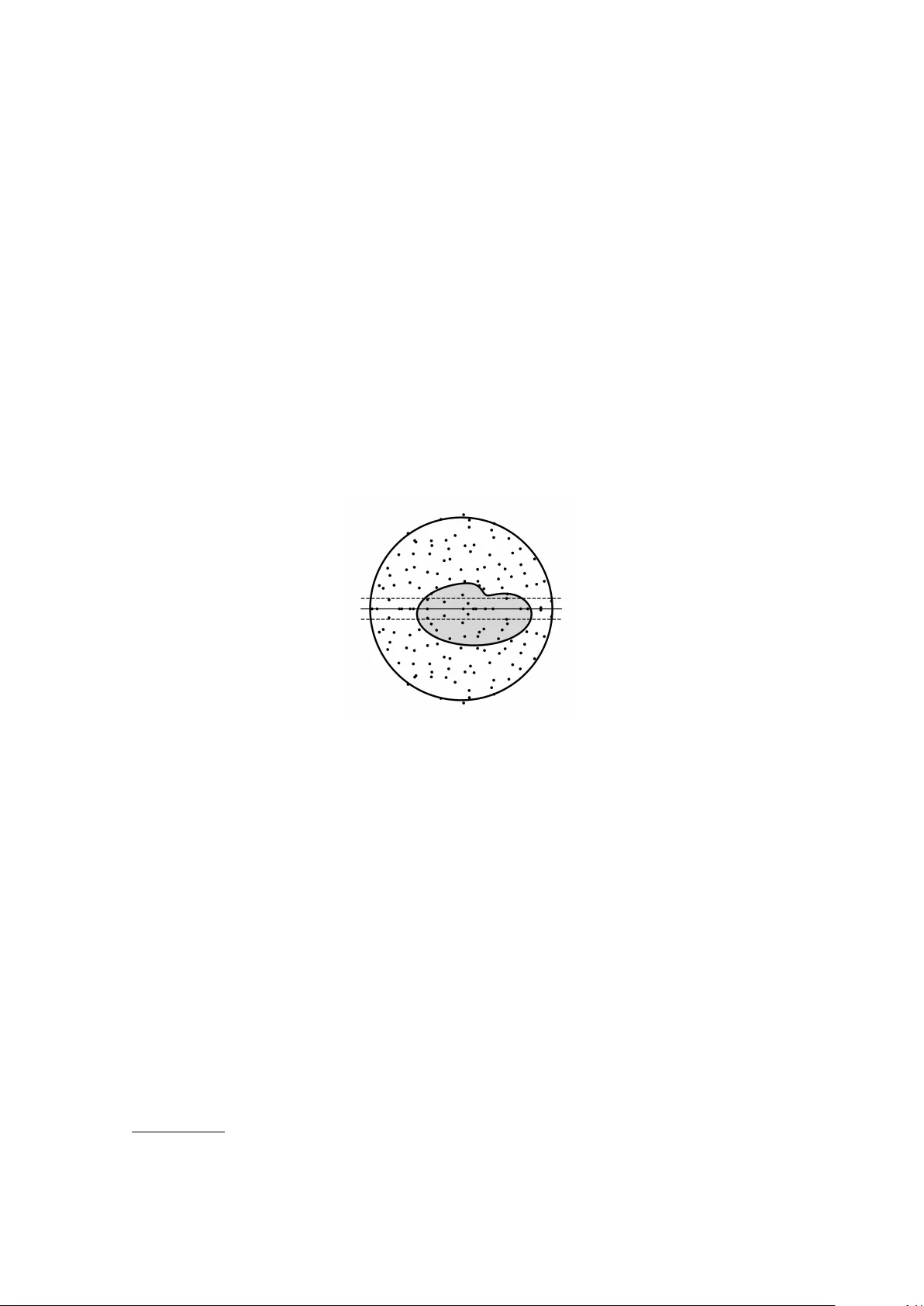
THE EIGENV ALUES OF I.I.D. MA TRICES ARE HYPERUNIFORM Giorgio Cipolloni * cipolloni@axp.mat.unir oma2.it László Erd ˝ os † ler dos@ist.ac.at Oleksii K olupaiev † okolupaiev@ist.ac.at A B S T R AC T . W e prove that the point process of the eigen values of real or complex non-Hermitian matrices X with independent, identically distributed entries is hyperuniform: the variance of the number of eigen values in a subdomain Ω of the spectrum is much smaller than the volume of Ω . Our main technical novelty is a very precise computation of the cov ariance between the resolv ents of the Hermitization of X − z 1 , X − z 2 , for two distinct complex parameters z 1 , z 2 . K eywor ds: Local Law , Zigzag Strategy , Dyson Brownian motion, Hyperuniformity , Girko’ s Formula, Linear Statistics. 2020 Mathematics Subject Classiﬁcation: 60B20, 82C10. C O N T E N T S 1. Introduction 2 Notations and con ventions 6 Acknowledgment 7 2. Main results 7 3. Proof strategy 9 3.1. Proof of Theorem 2.4 11 3.2. Ideas behind the proofs of Propositions 3.1 and 3.2 12 3.3. The real case 18 Outline of the paper 18 4. Local laws: set-up and results 19 4.1. Single-resolvent local la w 19 4.2. Nov el av eraged two-resolvent local la w 20 4.3. Multi-resolvent local la ws for longer chains 24 5. Calculations with the Girko’ s formula 25 5.1. Preliminary reductions in the Girko’ s formula 25 5.2. Calculation of the expectation: proof of Proposition 3.1 27 5.3. Upper bound on the variance: proof of Proposition 3.2 28 6. Proofs of the ingredients required for the analysis of the regime η ≲ N − 1 31 6.1. Proof of Proposition 3.5 32 6.2. Proof of Proposition 3.6 34 6.3. Proof of Proposition 3.7 37 7. Chaos expansion for co variance: Proof of Proposition 3.4 38 7.1. Initial expansion 39 7.2. Hierarchy of cov ariances: Proof of Proposition 7.2 43 7.3. Proof of the master inequalities in Proposition 7.3 45 Appendix A. Additional analysis of the matrix Dyson equation 49 A.1. 2-body stability analysis: Proof of Proposition 4.4 49 A.2. Bound on the propagator: proof of Lemma 4.3 52 Date : February 25, 2026. * Univ ersity of Rome T or V er gata, V ia della Ricerca Scientiﬁca 1, 00133 Rome, Italy . * Partially supported by the MUR Excellence Department Project MatMod@TO V awarded to the Department of Mathematics, Univ ersity of Rome T or V er gata, CUP E83C18000100006. † Institute of Science and T echnology Austria, Am Campus 1, 3400 Klosterneuburg, Austria. † Supported by the ERC Advanced Grant “RMTBe yond” No. 101020331. 1 2 HYPER UNIFORMITY A.3. Proof of Proposition 4.6 55 References 56 Supplementary Material 60 Section S1. Decorrelation for the Dyson Brownian motion 60 Section S2. Proof of the multi-resolvent local la ws from Section 4 64 S2.1. Proof of Proposition S2.4: bounds on the deterministic counterparts 68 S2.2. Proof of Proposition S2.5 72 S2.3. Proof of Proposition 4.8 83 S2.4. Proof of Proposition 4.2 for general b ∈ [0 , 1] 84 S2.5. Proof of Proposition 4.5 85 Section S3. The real case 85 S3.1. Proof of Theorem 2.6 88 S3.2. Proof of Proposition S3.5 90 S3.3. Proof of Proposition S3.1 91 S3.4. Proof of Propositions S3.2, S3.3 and S3.4 92 Section S4. Proofs of the additional technical results 95 S4.1. Relaxation of Assumption 2.3 95 S4.2. Proof of (5.40) 96 S4.3. Proof of (7.56) 97 S4.4. Proof of Lemma S2.8: properties of ˆ β 12 98 S4.5. Proof of Lemma S3.6 99 1. I N T R O D U C T I O N W e consider the i.i.d. matrix ensemble , i.e. an ensemble of N × N non-Hermitian random matrices X with independent, identically distributed (i.i.d.) real or complex centered entries. For con venience, we normalize the entries of X so that E | X ij | 2 = N − 1 . Then eigenv alues σ i of such matrices form a correlated point process on the unit disk of the complex plane; see [13, 51] for the Ginibre ensemble 1 and [27, 41, 73, 80] for general i.i.d. matrices (see also the recent [3, 18, 25, 71, 72, 97]). These eigen values tend to be uniformly distrib uted ov er the unit disk D . In particular , for any (suf ﬁciently nice) subdomain of the disk Ω ⊂ D , it is well kno wn [7, 52, 54, 82, 90] that ( cir cular law ) (1.1) N Ω := #  σ i ∈ Ω  = N X i =1 1 ( σ i ∈ Ω) = N | Ω | π + o ( N ) , with high probability . In particular , this implies E N Ω ∼ N . Note that the lhs. of (1.1) is random, while the leading order term in the rhs. is deterministic. It is then natural to study the ﬂuctuations around this deterministic limit. F or a system of independent particles, such as a Poisson point process it holds that the number variance is proportional to the e xpectation, i.e. V ar( N Ω ) ∼ E N Ω ∼ N . Thus, the natural question: Is the size of V ar( N Ω ) for i.i.d. matrices still proportional to those of the mean? W e answer it negativ ely; the number variance is much smaller than the e xpected size of N Ω : Theorem 1.1 (Informal statement) . Let X be an i.i.d. matrix and consider any nice domain Ω ⊂ D . Then, ther e exists a q > 0 such that (1.2) V ar( N Ω ) ≤ N 1 − q . Our proof explicitly gives q = 1 / 40 in the complex case and q = 1 / 106 in the real case, see Theo- rems 2.4 and 2.6 belo w . Theorem 1.1 establishes a connection between the point process of the eigen values of general i.i.d. matrices with hyperuniformity , a key concept in condensed matter physics for classify- ing crystals, quasicrystals, and exotic states of matter . In [93, Section 1], T orquato deﬁnes the concept of hyperuniformity as: 1 W e say that X belongs to the real/complex Ginibre ensemble if its entries are (normalized) standard real/complex Gaussian random variables. HYPER UNIFORMITY 3 (...) the number variance of particles within a spherical observation window of radius R gr ows more slowly than the window volume in the lar ge–R limit. For a system of independent particles the number variance is proportional to the volume V ar( N Ω ) ∼ N , hence it is not hyperuniform. Hyperuniformity is typically a signature of strong correlations at large distances in the system that reduce ﬂuctuations. In random matrix theory , one well-known manifestation of such correlations is the eigen value rigidity , pro ven in many Hermitian random matrix models, which asserts that each eigen value ﬂuctuates on a scale only slightly larger (by an N ϵ factor) than the typical distance between neighbouring eigen values. In particular , this trivially implies hyperuniformity in the sense of T orquato. In fact, for Hermitian models with eigenv alue rigidity , the variance of N I , the number of eigen values within an interv al I ⊂ R , is bounded by N ϵ , independently of I . Note that here the concept of rigidity uses that the Hermitian spectrum is one dimensional hence the eigenv alues can be ordered. For the same reason, the proof of eigen value rigidity easily follows from optimal concentration properties of the resolv ent ( optimal local laws ). In the tw o-dimensional setting of non-Hermitian random matrices, there is no direct concept of eigenv alue rigidity , but hyperuniformity can be interpreted as a higher dimensional version of the same strong correlations that cause rigidity . Ho wev er , in this case hyperuniformity does not simply follo w from optimal local la ws (which are well understood in this setting as well); substantial new inputs are needed. The word hyperuniformity was coined by T orquato and Stillinger [95] in the early 2000, analogous concepts appeared in the physics of Coulomb gases much earlier [60, 66, 68, 75, 76]. In recent years this phenomenon attracted lots of interest in a v ariety of models in mathematics and physics (here for concreteness we focus only on two-dimensional objects), including av eraged and perturbed lattices [50], zeroes of random polynomials with i.i.d. Gaussian coef ﬁcients [48, 87], in variant point processes in a plane [88], certain fermionic systems [17, 94], Berezin-T oeplitz operators in connection with the Quantum Hall Effect [19]. A rigorous proof of hyperuniformity in system with two-body interactions is notoriously difﬁcult. In the prominent model of the two-dimensional Coulomb gas (also known as the two-dimensional one component plasma) hyperuniformity was proved only very recently by Leblé [65]. This result showed that the number v ariance is bounded by N/ (log N ) a , for some small a > 0 ; so, in particular, it grows more slowly than the v olume N . Our result (1.2) sho ws that the point process gi ven by the eigenv alues of general non-Hermitian i.i.d. ma- trices is hyperuniform. It can thus be thought as a random matrix counterpart of [65], with a much stronger control on the number variance: we prove a polynomial f actor N q , while in the Coulomb gas model only a logarithmic factor (log N ) a was obtained. Pre vious to our result, in the random matrix setting, hyperunifor - mity was known only for integrable ensembles such as complex Ginibre matrices [40, 70, 69, 89] (see also the related works [1, 17, 49, 84], and the four moment matching result [92]), for real Ginibre matrices aw ay from the real axis [53] (see also [4] for the symplectic Ginibre ensemble), for elliptic Gaussian matrices and normal matrix models [5] (the latter result was later improved in [77]). In particular, our result is ne w ev en for real Ginibre matrices for domains Ω intersecting the real axis. Before e xplaining our strategy to prove (1.2), we point out that in certain systems a stronger version of hyperuniformity is expected. In the so-called “class I hyperuniform” systems, the number v ariance grows as the perimeter 2 , which is the slo west possible gro wth (see e.g. [11]), and not merely slo wer than the volume. In particular , for point process in two-dimensions, “class I hyperuniform” means that V ar( N Ω ) ∼ √ N . This strong version of hyperuniformity has been proven for Ginibre ensembles using explicit formulas. The two-dimensional Coulomb gas is also expected to be “class I hyperuniform”, but the result [65] is still far from catching this. Similarly to these examples, it is expected that the eigen values σ i for general i.i.d. matrices form also a “class I hyperuniform” system, i.e. that V ar( N Ω ) ∼ √ N . Our result giv es the ﬁrst (and effecti ve) proof of hyperuniformity for the i.i.d. random matrices, howe ver , (1.2) is also very far from the (expected) optimal √ N bound. W e leave this for future work. Howe ver , we mention that our result also covers certain mesoscopic N -dependent domains Ω N ⊂ D (see Assumption 2.3 below), showing that hyperuniformity occurs on mesoscopic scales as well. 2 W e point out that initially this was chosen as the deﬁnition of hyperuniformity in [95]. 4 HYPER UNIFORMITY T o study the variance of N Ω , we view it as a special case of (centered) linear statistics 3 (1.3) L N ( f ) := N X i =1 f ( σ i ) − E N X i =1 f ( σ i ) , when f ( · ) = 1 ( · ∈ Ω) . In particular , N Ω − E N Ω = L N ( f ) , for this choice of f . W e thus need to giv e a bound on the variance of L N ( f ) for f ( · ) = 1 ( · ∈ Ω) . The behavior of the linear statistics L N ( f ) is very well understood for smooth (e.g. C 2 ) test functions [33, 29, 35, 63, 85, 86] (see also [79]), howe ver extending this study to less regular f ’ s creates substantial dif ﬁculties. In particular , the loss of regularity of f does not only present new technical complications, but it substantially changes the answer . In fact, it is expected that the size of the number variance is much bigger than V ar( L N ( f )) for smooth f . More precisely , as mentioned abov e, it is expected that V ar( N Ω ) ∼ √ N , while it is proven in [33, Theorem 2.2] that for smooth test functions the linear statistics hav e an order one variance (1.4) V ar( L N ( f )) = V f + o (1) , V f := 1 4 π 2 Z D |∇ f ( z ) | 2 d 2 z + κ 4     1 π Z D f ( z ) d 2 z − 1 2 π Z 2 π 0 f ( e i θ ) d θ     2 , where κ 4 is the fourth cumulant of the entries of X . Note that (1.4) is consistent with the fact that if we regularized 1 ( · ∈ Ω) on a scale ∼ N − 1 / 2 (which is the ﬂuctuation scale of the eigenv alues of X ) and naiv ely plug this regularized f in the formula (1.4) for V f , we would indeed get a size of order V f ∼ √ N . T o regularize the indicator function we rely on the Portmanteau principle (see Assumption 2.3 belo w), which for the variance states (1.5) V ar( N Ω ) ≲ V ar( L N ( f + )) + V ar( L N ( f − )) +  E L N ( f + ) − E L N ( f − )  2 . Here f ± are the lo wer and upper en velope functions with f − ≤ 1 Ω ≤ f + and they are chosen to be smooth on a scale N − a , for a certain a > 1 / 2 which we will then optimize. While it seems natural to smooth out 1 ( · ∈ Ω) on a scale ∼ N − 1 / 2 (i.e. at the ﬂuctuation scale of the eigen values), in practice we will need to choose a smaller scale N − a , with some a > 1 / 2 , to make sure that the term ( E L N ( f + ) − E L N ( f − )) 2 is negligible compared to the upper bound on the other two terms in the rhs. of (1.5). In particular , this additional term represents the discrepancy in the number of eigen values in the support of the functions 1 Ω and f ± . Choosing a sufﬁciently large, the bound (1.5) enables us to reduce (1.2) to study the linear statistics of f ± , which are smooth, ev en if only on the very small scale N − a . T o study these eigenv alue statistics we rely on Girko’ s formula (1.7) below , a backbone in the study of non-Hermitian spectral statistics. The key feature of this formula is that it relates the eigenv alues of any non-Hermitian matrix X with those of a family of Hermitized matrices (1.6) H z :=  0 X − z ( X − z ) ∗ 0  , z ∈ C . Then, Girko’ s formula reads as (1.7) N X i =1 f ( σ i ) = i 4 π Z C ∆ f ( z ) Z ∞ 0 T r G z (i η ) d η d 2 z , G z (i η ) := ( H z − i η ) − 1 , for any smooth function f . From the appearance of ∆ f in (1.7) it is clear that the smoothness of f is extremely relev ant to control the eigen value statistics. For our approximating functions f = f ± from abo ve we will use the bound ∥ ∆ f ∥ ∞ ≤ N 2 a , which grows v ery quickly as a > 1 / 2 . T o deduce from (1.5) and (1.7) that the eigen value process of X is hyperuniform in the sense that the lhs. of (1.2) has an upper bound of order N 1 − ξ for some tiny implicit constant ξ > 0 , it sufﬁces to show with the same implicit level of precision that the spectra of H z 1 and H z 2 decorrelate on all scales | z 1 − z 2 | ≫ N − 1 / 2 . Such weak inputs are already av ailable from [33]. Howe ver , along this approach, not only any explicit v alue of ξ is practically untraceable, but also the actual proof theoretically would yield an exponent ξ which depends on the model parameters in Assumption 2.1 belo w , such as the constants in the upper bounds on the moments of the single-entry distrib ution of X . In contrast, in this paper we get the univ ersal quantitativ e exponent in (1.2), which requires substantial new inputs. In particular , we need 3 The linear statistics for f ( · ) = 1 ( · ∈ Ω) are often called counting statistics . HYPER UNIFORMITY 5 to quantify all spectral decorrelation rates in terms of powers of | z 1 − z 2 | , which is achie ved by performing the analysis that we now e xplain. For more details see the comment belo w Proposition 3.2. T o analyze the rhs. of (1.7) it is conv enient to split the η -integral into three regimes: sub-micr oscopic r e gime ( η ≪ 1 / N ), micr oscopic re gime ( η ∼ 1 / N ), and macr o-mesocopic r egime ( η ≫ 1 / N ). They re- quire dif ferent methodological approaches. Inspired by [33], we can control the size of the sub-microscopic and microscopic regimes using left-tail bounds on the smallest singular value of X − z from [12, 91] (see also [39, 31]) and the Dyson Bro wnian motion (DBM) from [14, 33], respectiv ely . The main novelty of this work lies in the analysis of the regime η ≫ 1 / N , where substantially higher precision, compared to previous w orks, is required. In order to compute the variance of L N ( f ) using (1.7), we naturally need to compute 4 Co v( ⟨ G 1 ⟩ , ⟨ G 2 ⟩ ) , where G i := G z i (i η i ) . The ﬁrst natural approach to compute Cov( ⟨ G 1 ⟩ , ⟨ G 2 ⟩ ) is to rely on similar com- putations to [33, Section 6]. Howe ver , the precision of [33, Eq. (6.31)] would gi ve (here η ∗ := η 1 ∧ η 2 ) (1.8) Co v( ⟨ G 1 ⟩ , ⟨ G 2 ⟩ ) = Main T erm N 2 + O  1 √ N η ∗ ( N η 1 η 2 ) 2  . The key drawback of (1.8) is that while the "Main T erm" in (1.8) behaves like | z 1 − z 2 | − 4 (see e.g. [33, Eq. (4.24)]), this decorrelation decay in | z 1 − z 2 | is not reﬂected in the error term. The decorrelation phenomenon is essential to prove a good estimate since the v ariance of L N ( f ) based upon (1.7) in volves a double d 2 z 1 d 2 z 2 integral of Co v ( ⟨ G 1 ⟩ , ⟨ G 2 ⟩ ) . The main technical result of this work is an improv ed co v ariance control, which in the Ginibre case gives (1.9) Co v( ⟨ G 1 ⟩ , ⟨ G 2 ⟩ ) = Main T erm N 2 + O  1 N [ | z 1 − z 2 | 2 + η 1 + η 2 ]( N η 1 η 2 ) 2  . Note that the error term in (1.9) does not only improv e (1.8) in terms of | z 1 − z 2 | , but also the N -po wer is better (e.g. N − 5 / 2 vs. N − 3 ). In addition, we prove (1.9) not only for spectral parameters on the imaginary axis but for all spectral parameters w 1 , w 2 in the bulk spectrum of H z 1 , H z 2 (in which case an additional regularizing term depending on the distance between w 1 and w 2 appears). In contrast, the pre vious results in [33] cov ered only spectral parameters along the imaginary axis. T o prove (1.9), we use a chaos e xpansion strategy , which consists in performing iterati ve cumulant expansions in Cov( ⟨ G 1 ⟩ , ⟨ G 2 ⟩ ) . More precisely , we start with a trivial bound of order ( N η 1 η 2 ) − 1 on the error term in the rhs. of (1.9), which simply follo ws by the single resolvent local law (see e.g. (4.1) below). Then, at each step of the chaos expansion we improve this bound by a (small) factor of ( N η ∗ ) − 1 . In the mesoscopic regime η ∗ ≥ N − 1+ ϵ , this factor is much smaller than one, howe ver it gains only N − ϵ for a small ϵ > 0 . Thus, the factor ( N [ | z 1 − z 2 | 2 + η 1 + η 2 ]) − 1 in the rhs. of (1.9) cannot in general be obtained in one step of this iteration. This forces us to perform iterativ e expansions, each expansion amounting to a further gain N − ϵ , until we reach the desired precision in (1.9). This gradual improv ement of the bound on the error term to reach the one in the rhs. of (1.9) in volv es understanding the size of more complicated cov ariances, which generalize the lhs. of (1.9). For example, the ﬁrst step generates (1.10) Co v  ⟨ G 1 − M 1 ⟩⟨ ( G 1 − M 1 ) M 2 1 ⟩ , ⟨ G 2 ⟩  , where M 1 is a certain deterministic approximation to G 1 introduced later in (3.30). These cov ariances are further subjected to the iterativ e expansions, giving rise to an entire hierarchy of more and more in volv ed cov ariances. Howe ver , they still hav e a speciﬁc structure that plays an important role in the analysis. Though the number of steps in the chaos e xpansion may be arbitrarily large, we will need to iterate the expansion roughly 1 /ϵ -times, where ϵ is the small parameter in the constraint η 1 ∧ η 2 ≥ N − 1+ ϵ . Ho wev er , at the end, the hierarchy of cov ariances needs to be truncated, meaning that we estimate these quantities arising after the ﬁnal step of the chaos expansion simply by size, without re-expanding them further . The loss in this size estimate is compensated by the many 1 / ( N η ∗ ) factors accumulated along the iteration. This size bound is giv en by the multi-r esolvent local laws : concentration bounds for the products of resolvents and deterministic matrices sandwiched in between (see Section 4 below). A related strategy was used in [55] to compute the covariance Cov( ⟨ G 1 ⟩ , ⟨ G 2 ⟩ ) for resolvents G j := ( W − w j ) − 1 , j = 1 , 2 , of a W igner matrix W . Our analysis of the Hermitized matrix H z carries three 4 For a matrix A ∈ C d × d we use the short-hand notation ⟨ A ⟩ = 1 d T r[ A ] . 6 HYPER UNIFORMITY nov elties, besides several technical complications. First, most importantly , G 1 and G 2 in [55] hav e the same spectral resolution, since they are resolvents of the same matrix W . This allows for a substantial simpliﬁcation of the structure of the hierarchy of covariances using the resolv ent identity G 1 G 2 = ( G 1 − G 2 ) / ( w 1 − w 2 ) , which also automatically giv es the decorrelation factor w 1 − w 2 . Since there is no analogous resolvent identity for products of resolvents of H z 1 and H z 2 with z 1  = z 2 , hence the decorrelation factor ( N [ | z 1 − z 2 | 2 + η 1 + η 2 ]) − 1 does not appear automatically . Instead, it will be obtained from the very reﬁned bound in a new two-resolvent local law for quantities of the form ⟨ G 1 B 1 G 2 B 2 ⟩ with deterministic matrices B 1 , B 2 (see Proposition 4.2 below). Second, the precision in the estimate of the error term in the chaos expansion is governed by the in verse of the so-called one-body stability operator B 11 introduced later below (4.7). In [55] this operator has a bounded inv erse, while in our setup it is unstable and the norm of B − 1 11 blows up as η − 1 1 for small η 1 ’ s. Thus, showing that this deterioration of the stability bound does not affect the ﬁnal result (1.9) requires a separate structural analysis of the hierarchy of cov ariances. Third, M 1 appearing in (1.10) is a multiple of identity in [55], while now it is an (2 N ) × (2 N ) matrix with a 2 × 2 block-constant structure. In particular, quantities arising along the chaos expansion contain traces of the form ⟨ G 1 B 1 G 1 · · · G 1 B k ⟩ for all k ∈ N and deterministic matrices B j , j ∈ [ k ] , with 2 × 2 block-constant structure, while in [55] such traces were automatically simpliﬁed to ⟨ G k 1 ⟩ . As a standard consequence of the new a veraged tw o-resolvent local law mentioned in the pre vious para- graph, we get the follo wing optimal (in N ) bound on the ov erlap of singular v ectors of X − z 1 and X − z 2 in the bulk re gime, i.e. for | z 1 | , | z 2 | ≤ 1 − δ , (1.11)   ⟨ u z 1 i , u z 2 j ⟩   2 +   ⟨ v z 1 i , v z 2 j ⟩   2 ≲ 1 N 1 | z 1 − z 2 | 2 + N − 1 | i − j | , with very high probability up to a factor N ξ , for an arbitrary small ξ > 0 . For a precise statement see Proposition 4.6. Here u z i and v z i are the left and right singular vectors associated to the i -th singular v alue of X − z . The main feature of (1.11) is the identiﬁcation of the decorrelation in | i − j | for all i, j , on top of the | z 1 − z 2 | 2 correlation decay that was kno wn before b ut only for | i | , | j | ≲ N ξ , see [20, Corollary 3.6]. A bound analogous to (4.23) w as obtained in [23, Theorem 2.6] for the o verlap of eigen vectors of W + D 1 and W + D 2 , where W is a Wigner matrix and D j = D ∗ j are deterministic deformations for j = 1 , 2 . In [23], ⟨ ( D 1 − D 2 ) 2 ⟩ played the role of | z 1 − z 2 | 2 in (1.11), while further improv ements beyond this quadratic bound were encoded in a complicated control parameter coined as the linear term , see [23, Eq.(2,17)]. In the current paper we encounter a similar control parameter (see the second line of (3.36) later). Owing to the more explicit structure of our model compared to [23], we manage to analyze precisely this control parameter and to extract from it the | i − j | contribution. W e note that the term | z 1 − z 2 | 2 in (4.23) plays an essential role in our analysis of the critical regime η ∼ N − 1 in the Girko’ s formula (1.7), and allows us to quantify the error terms coming from the Dyson Brownian motion technique. Meanwhile, the | i − j | decay in the rhs. of (1.11) is a result of an independent interest which is not used in the proof of Theorem 1.1. Notations and con ventions. W e set [ k ] := { 1 , ..., k } for a positi ve integer k ∈ N and ⟨ A ⟩ := d − 1 T r( A ) , d ∈ N , for the normalized trace of a d × d matrix A . Additionally , we denote its transpose by A t . The sets of real and complex numbers are denoted by R and C , respectiv ely , while D ⊂ C stands for the open unit disk. F or a ﬁnite set S we denote the number of elements in S by # S . F or positive quantities f , g we write f ≲ g , f ≳ g , to denote that f ≤ C g and f ≥ cg , respecti vely , for some N -independent constants c, C > 0 that depend only on the basic control parameters of the model in Assumptions 2.1 and 2.3 belo w . In informal explanations we sometimes use the notation f ≪ g , which indicates that f is "much smaller" than g . W e denote vectors by bold-faced lower case Roman letters x , y ∈ C d , for some d ∈ N . Moreov er , for vectors x , y ∈ C d and a matrix A ∈ C d × d we deﬁne ⟨ x , y ⟩ := d X i =1 ¯ x i y i , A xy := ⟨ x , A y ⟩ . Matrix entries are indexed by lo wer case Roman letters a, b, c, ..., i, j, k , ... from the be ginning or the middle of the alphabet. HYPER UNIFORMITY 7 The cov ariance of two complex-v alued random variables ζ 1 and ζ 2 is denoted by Co v( ζ 1 , ζ 2 ) := E  ( ζ 1 − E ζ 1 )( ζ 2 − E ζ 2 )  . W e further denote the variance of a complex-valued random variable ζ by V ar[ ζ ] := Cov( ζ , ζ ) . For a pair of real or complex-valued stochastic processes X = X ( t ) and Y = Y ( t ) , we denote their cov ariation process by [ X, Y ] t . Finally , we will use the concept with very high pr obability , meaning that for any ﬁxed D > 0 , the probability of an N -dependent event is bigger than 1 − N − D for all N ≥ N 0 ( D ) . W e will use the con vention that ξ > 0 denotes an arbitrarily small positiv e exponent, independent of N . Moreov er , we introduce the common notion of stochastic domination (see, e.g., [44]): For two f amilies X =  X ( N ) ( u ) | N ∈ N , u ∈ U ( N )  and Y =  Y ( N ) ( u ) | N ∈ N , u ∈ U ( N )  of non-negati ve random v ariables inde xed by N , and possibly a parameter u , we say that X is stochastically dominated by Y , if for all ϵ, D > 0 we have sup u ∈ U ( N ) P h X ( N ) ( u ) > N ϵ Y ( N ) ( u ) i ≤ N − D for large enough N ≥ N 0 ( ϵ, D ) . In this case we write X ≺ Y . If for some complex family of random variables we ha ve | X | ≺ Y , we also write X = O ≺ ( Y ) . Acknowledgment. W e thank Leslie Molag for comments on the existing literature and for the references [69, 77, 88]. 2. M A I N R E S U L T S W e consider r eal or complex i.i.d. matrices X , i.e. N × N matrices whose entries x ab d = N − 1 / 2 χ are independent and identically distrib uted. W e impose the following assumptions on the (possibly N - dependent) complex-v alued random variable χ . Assumption 2.1. (i) The random variable χ satisﬁes E χ = 0 , E | χ | 2 = 1 . In addition, in the comple x case we also assume E χ 2 = 0 . W e further assume the existence of high moments, i.e . that ther e exist constants C p > 0 , for any p ∈ N , such that (2.1) E | χ | p ≤ C p . (ii) Ther e exist a (small) a > 0 and a (larg e) b > 0 suc h that the pr obability density ρ χ of χ satisﬁes (2.2) ρ χ ∈ L 1+ a ( C ) , ∥ ρ χ ∥ 1+ a ≤ N b . Remark 2.2. W e use the mild re gularity assumption (2.2) only to contr ol the η ≤ N − 100 r e gime in the Girko’ s formula (1.7) . This assumption can easily be r emoved by standard methods as intr oduced in [92] (see also [36, Remark 2.2] ), we omit the details for br evity and to k eep the pr esentation simpler . Denote the eigen values of X by { σ i } N i =1 . For any test function g : C → C , the linear eigen value statistics of X is giv en by L N ( g ) := N X i =1 g ( σ i ) . T ypically , the smoother is the test function g the simpler is the analysis of L N ( g ) (see e.g. the paragraph below (1.7)). As explained in the introduction, to study the phenomenon of hyperuniformity we need to consider the test function g being the indicator function of a (possibly N -dependent) subset Ω = Ω N of the disk. Howe ver , all the existing results on the linear eigen value statistics assume at least that g ∈ H 1 ( C ) , i.e. do not cover our case. W e consider domains Ω N satisfying the following assumptions: Assumption 2.3. The domain Ω N ⊂ C is open and simply connected, with C 2 boundary . Ther e exists δ > 0 such that Ω N ⊂ (1 − δ ) D for all N ∈ N . Ther e further e xists an exponent α ∈ [0 , 1 / 2) , such that Ω N = N − α e Ω N , wher e (2.3) diam( e Ω N ) := sup {| z 1 − z 2 | : z 1 , z 2 ∈ e Ω N } ∼ 1 , and the curvatur e of the boundary ∂ e Ω N is bounded fr om above uniformly in N . 8 HYPER UNIFORMITY W e are now ready to formulate our main result in the comple x case. Theorem 2.4 (Complex case) . Let X be a complex N × N i.i.d. matrix satisfying Assumption 2.1. Fix α ∈ [0 , 1 / 2) and let Ω N ⊂ D be a domain satisfying Assumption 2.3 with exponent α . Then, ther e exists q 0 > 0 such that for any ﬁxed ξ > 0 we have (2.4) V ar [# { σ i : σ i ∈ Ω N } ] ≤ N 1 − 2 α − q 0 (1 / 2 − α )+ ξ for sufﬁciently lar ge N . Our pr oof gives 5 q 0 = 1 / 20 . T o state the analogue of Theorem 2.4 in the real case, we impose the follo wing additional assumption on the domain Ω N . Assumption 2.5. In the set-up of Assumption 2.3 we assume that the angle between the tangent line to e Ω N at these points and the real axis is at least φ 0 , for some N -independent φ 0 > 0 . W e further assume that ther e exists a (small) N -independent constant d 0 > 0 such that ∂ e Ω N ∩ { z : |ℑ z | ≤ d 0 } is either empty or consists only of curves intersecting the r eal axis. In other words, Assumption 2.5 guarantees that if Ω N intersects the real axis, then this happens trans- versely , cf. Figure 1. It also prohibits ∂ Ω N to concentrate in a neighborhood of the real axis of a radius much smaller than the scale of Ω N . F I G U R E 1 . In gray , we illustrated a macroscopic ( α = 0 ) domain Ω N in the case when it intersects the real line. The dashed lines correspond to ℑ z = ± d 0 , where d 0 is given by Assumption 2.5. In this example, the intersection of ∂ Ω N and the set |ℑ z | ≤ d 0 consists of two curves transv ersely intersecting the real axis. Finally , the scattered dots depict the eigen values of a large real i.i.d. matrix X . Theorem 2.6 (Real case) . Let X be a r eal N × N i.i.d. matrix satisfying Assumption 2.1. F ix α ∈ [0 , 1 / 2) and let Ω N ⊂ D be a domain satisfying Assumptions 2.3 and 2.5 with an exponent α . Then, there exist q 0 , q 1 > 0 such that for any ﬁxed ξ > 0 we have (2.5) V ar [# { σ i : σ i ∈ Ω N } ] ≤ N 1 − 2 α − q 0 (1 / 2 − α )+ ξ + N 1 − 2 α − q 1 + ξ for sufﬁciently lar ge N . Our pr oof gives q 0 = 1 / 20 and q 1 = 1 / 106 . Remark 2.7. W e now discuss several possible e xtensions of the r esults in Theorems 2.4 and 2.6. (i) [Relaxation of Assumption 2.3]. W e stated Theorem 2.4 under the assumption that the boundary of Ω N is a C 2 curve. However , a car eful examination of our proof shows that this assumption can be relaxed: one can allow ∂ Ω N to be a piecewise C 2 curve. In particular , Ω N can be a r ectangle whose edges have length of or der N − α . F or mor e details see Supplementary Section S4.1. Similarly , Assumption 2.3 can be r elaxed in Theorem 2.6, but only away fr om the real axis. T o avoid technicalities, we only mention that if Ω N does not intersect the r eal axis and lies at a distance of order N − α fr om it, then the discussion in Supplementary Section S4.1 applies also in the r eal case. 5 See Remark 2.7–(v) for possible improvements on q 0 . HYPER UNIFORMITY 9 (ii)[Relaxation of Assumption 2.5]. In the case when Ω N does not inter sect the real axis, Assumption 2.5 r equir es Ω N to be at distance at least of or der N − α fr om the r eal axis. Our methods allow to tr eat a more general case when the distance fr om Ω N to R is at least N − θ for any ﬁxed 0 ≤ θ < 1 / 2 , and give a quantitative impr ovement of the volume law bound N 1 − 2 α on the lhs. of (2.5) . However , we r efrain fr om computing the exact e xponents in this generalized setting. (iii)[Domains overlapping the edge]. In Theorems 2.4 and 2.6 we focused on domains Ω N well inside the unit disk. However , an analogous pr oof would also work for domains overlapping the edge of the spectrum (i.e. the unit cir cle). The main ne w difﬁculty is that in this r e gime the local laws and the covariance expansion in Sections 4 and 7 would need to be extended to the r e gime | z | ≈ 1 , when the limiting eigen value density of H z develops a cusp singularity . The methods of Section 7 and Supplementary Section S2 are str ong enough to cover this r egime as well, however , at the price of mor e tec hnically in volved computations. F or these r eason we decide to omit the edge r e gime from the pr esentation. (iv)[Bounds on higher moments]. In Theorems 2.4 and 2.6 we estimate the variance of the number of eigen values in Ω N , since this is the quantity determining whether a point pr ocess is hyperuniform or not. Our methods also allow us to show that the p -th moment, p ∈ N , of this random variable is much smaller than N (1 / 2 − α ) p , and to quantify this smallness. (v)[Possible improvements on q 0 , q 1 ]. In Theorems 2.4 and 2.6 the exponents q 0 , q 1 ar e not optimal. By performing a more careful analysis, one could increase the value of q 0 to 1 / 3 and remove the term containing q 1 in the rhs. of (2.5) . Howe ver , this result will be still far fr om the optimal one corr esponding to q 0 = 1 . F or mor e details see comments below Pr opositions 3.5, 3.7, and in Section 3.3. 3. P R O O F S T R AT E G Y T o keep the presentation simpler, we now only consider the complex case. W e will then explain the minor required dif ferences for the real case in Section 3.3. In this section we discuss the main ideas of the proof of Theorem 2.4. T o study linear statistics with the test function being a sharp cut-of f in Theorem 2.4, we approximate it by smooth functions. T o this end, we consider a smooth bump function ω satisfying (3.1) ω : C → [0 , + ∞ ) , ω ∈ C ∞ c ( C ) , Z C ω ( z )d 2 z = 1 and supp( ω ) = D , and rescale it as ω a,N ( z ) := N 2 a ω ( N a z ) , ∀ z ∈ C , for some a > 0 . Note that ω a,N integrates to 1. W e then consider the con volution (3.2) f a,N := ϕ N ∗ ω a,N , for a characteristic function ϕ N of an appropriately chosen subset of the unit disk, which may slightly differ from Ω N . Speciﬁcally , in the proof of Theorem 2.4 we will construct this domain by adding a small neighborhood of ∂ Ω N to Ω N , or by removing it from Ω N (see (3.10) belo w). Ho wev er , the exact construction is not important at this moment. By a Portmanteau-type argument (see Lemma 3.3 below), approximating the characteristic function of Ω N both from abo ve and below by functions of the form (3.2), we reduce (2.4) to the analysis of expectation and v ariance of L N ( f a,N ) . Linear eigenv alue statistics with a test function of the form ω ( N a ( z − z 0 )) , for some z 0 ∈ C , has been e xtensiv ely studied in the macr oscopic regime ( a = 0 ) [33, 29], and in the entire mesoscopic regime ( 0 < a < 1 / 2 ) [35]. For instance, for 0 < a < 1 / 2 it is known from [35, Theorem 2.1] that for | z 0 | ≤ 1 − τ with an y ﬁx ed τ > 0 , the v ariance of L N ( ω ( N a ( z − z 0 ))) is of order one. This is a consequence of the fact that the eigen values of i.i.d. matrices are “rigid" in the unit disk. Our setting differs from that of [35] in two fundamental aspects. First, to approximate the characteristic function of Ω N by f a,N with precision sufﬁcient for (2.4), we are forced to take a > 1 / 2 , i.e. we need to consider sub-microscopically localized test functions. In this regime, L N ( ω ( N a ( z − z 0 ))) is gov erned by the ﬁnitely many eigen values of X closest to z 0 , so the self-averaging mechanism no longer applies. Second, the test function f a,N naturally li ves on two scales: a mesoscopic scale N − α ≫ N − 1 / 2 , corre- sponding to the diameter of Ω N , and the sub-microscopic smoothing scale N − a ≪ N − 1 / 2 . This two-scale structure requires to understand quite precisely the correlation between eigen values of X near z 1 and z 2 , for mesoscopically separated z 1 , z 2 . 10 HYPER UNIFORMITY The difﬁculties discussed above pre vent us from computing the leading order behavior of the variance of L N ( f a,N ) , as it was done for smooth test functions in the mesoscopic scaling in aforementioned [35, Theorem 2.1] and in the macroscopic scaling (i.e. for an N -independent test function) in [33, Theorem 2.2] and [29, Theorem 2.2]. Nevertheless, we establish an effecti ve upper bound on the variance of L N ( f a,N ) in Proposition 3.2. W e also compute the expectation of this linear statistics up to the leading order for an explicit range of a ’ s above the critical scale 1 / 2 ( i.e. for sub-microscopic scales), see Proposition 3.1. T ogether Propositions 3.1 and 3.2 serve as the main ingredients in the proof of Theorem 2.4. No w we discuss these results in more detail, starting with the computation of the expectation. For simplicity of presentation, we consider the case when ϕ N in (3.2) is the characteristic function of Ω N . Since we impose only Assumption 2.3 on Ω N , this restriction yields no loss of generality . T o compute E L N ( f a,N ) , it is more con venient to work not directly with f a,N but with the test function (3.3) ω ( z 0 ) a,N ( z ) := ω a,N ( z − z 0 ) = N 2 a ω ( N a ( z − z 0 )) , z , z 0 ∈ C , which serv es as a more basic object compared to f a,N , as the expectation of f a,N can be easily recovered once the expectation of ω ( z 0 ) a,N is kno wn (see (3.4) below). In particular , (3.3) does not carry any information about Ω N , which is though encoded in f a,N . Once the expectation of the linear statistics with the test function (3.3) has been computed, integrating it o ver z 0 ∈ Ω N yields E L N ( f a,N ) , i.e. (3.4) E L N ( f a,N ) = Z Ω N E L N ( ω ( z 0 ) a,N )d 2 z 0 . Although the assumptions imposed on ω in (3.1) are essential for the proof of Theorem 2.4, some of them are not needed for the computation of e xpectation of the linear statistics. In the following proposition we therefore relax (3.1) and, in particular , allow ω to be complex-v alued. Proposition 3.1. Let X be a complex N × N i.i.d. matrix satisfying Assumption 2.1. F ix δ > 0 , a ∈ [1 / 2 , 1 / 2 + ν 0 ) with ν 0 := 1 / 14 , and let ω ∈ C 2 c ( C ) be a complex-valued function with integr al 1. Uniformly in z 0 ∈ D with | z 0 | ≤ 1 − δ it holds that (3.5) E L N  ω ( z 0 ) a,N  = N π  1 + O ( N − c )  for some c > 0 , wher e ω ( z 0 ) a,N is deﬁned in (3.3) . F ix additionally α ∈ [0 , 1 / 2) . Let Ω N ⊂ D be an N -dependent domain satisfying Assumption 2.3 with exponent α and let f a,N be deﬁned as in (3.2) with ϕ N equal to the test function of Ω N . Then we have (3.6) E L N  f a,N  = N | Ω N | π  1 + O ( N − c )  , wher e | Ω N | is the volume of Ω N . W e remark that the follo wing analogue of (3.5) is kno wn from [35, Eq.(2.5)] in the mesoscopic regime 0 < a < 1 / 2 under slightly more general assumptions on ω : (3.7) E L N  ω ( z 0 ) a,N  = N π Z ω ( z )d 2 z + N 2 a 8 π Z C ∆ ω ( z )d 2 z + O (1 + N 2 a − c ) , for some ﬁxed c > 0 . In (3.5) there is no analogue of the second term in the rhs. of (3.7), since the integral of ∆ ω over the entire complex plane v anishes due to the smoothness and compact support of ω . Meanwhile, the ﬁrst term in the rhs. of (3.7) exactly corresponds to the leading term in the rhs. of (3.5). As it was discussed around (3.4), (3.6) immediately follo ws from (3.5), so (3.6) is stated only for com- pleteness. W e also included a = 1 / 2 into Proposition 3.1, since the methods developed in this paper for the regime a > 1 / 2 also apply to this case. Ho wev er, Proposition 3.1 is not used for a = 1 / 2 in the proof of Theorem 2.4. The same remark applies to the following bound on the variance of L N ( f a,N ) stated for all a ≥ 1 / 2 . Proposition 3.2. Assume the set-up and conditions of Pr oposition 3.1, b ut instead of a ∈ [1 / 2 , 1 / 2 + ν 0 ) consider any ﬁxed a ≥ 1 / 2 . Then it holds that (3.8) V ar [ L N ( f a,N )] ≲ N 2( a − α ) − 2 q 0 (1 / 2 − α )+ ξ for any ﬁxed ξ > 0 , where q 0 := 1 / 20 . HYPER UNIFORMITY 11 From the Girko’ s formula (1.7) we have (3.9) V ar [ L N ( f a,N )] = N 2 (4 π ) 2 Z C Z C ∆ f ( z 1 )∆ f ( z 2 ) Z ∞ 0 Z ∞ 0 Co v ( ⟨ G z 1 (i η 1 ) ⟩ , ⟨ G z 2 (i η 2 ) ⟩ ) d η 1 d η 2 d 2 z 1 d 2 z 2 . The single-resolv ent local law (see (3.34) belo w) gi ves an upper bound of order ( N 2 η 1 η 2 ) − 1 on the covari- ance in the rhs. of (3.9), up to an N ξ factor . This leads to the upper bound of order N 2( a − α )+ ξ on the lhs. of (3.8). Proposition 3.2 thus consists in a quantitative impro vement of this elementary bound. The remainder of this section is or ganized as follo ws. In Section 3.1 we prove Theorem 2.4 relying on Propositions 3.1 and 3.2. In Section 3.2 we then summarize the technical ingredients required for the proofs of these results. Additionally , we e xplain the origin of the constants ν 0 and q 0 appearing in the statements of Propositions 3.1 and 3.2, respectiv ely . 3.1. Proof of Theorem 2.4. From no w on, we take ω to be a bump function , meaning that ω satisﬁes (3.1). Fix an exponent a ∈ [1 / 2 , 1 / 2 + ν 0 ) with ν 0 = 1 / 14 , at the end we will optimize the estimates over a . Deﬁne (3.10) Ω − N :=  z ∈ Ω N : d( z , ∂ Ω N ) > N − a  , Ω + N :=  z ∈ C : d( z , Ω N ) < N − a  , where d( · , · ) is the Euclidean distance in C . It is easy to see that the Assumption 2.3 imposed on Ω N implies that Ω − N and Ω + N also satisfy 6 Assumption 2.3. Recall the notation ϕ N for the characteristic function of Ω N and denote the characteristic functions of Ω − N and Ω + N by ϕ − N and ϕ + N , respectiv ely . Denote further (3.11) f ± a,N := ϕ ± N ∗ ω a,N . Since ω is supported on the unit disk, the construction (3.10) implies that (3.12) f − a,N ( z ) ≤ ϕ N ( z ) ≤ f + a,N ( z ) , ∀ z ∈ C . Now we formulate a simple statement allowing us to get an upper bound on the v ariance of L N ( ϕ N ) in terms of the ﬁrst two moments of L N ( f ± a,N ) . Lemma 3.3 (Portmanteau principle) . F or any N ∈ N it holds that (3.13) V ar [ L N ( ϕ N )] ≤ 2  V ar h L N ( f + a,N ) i + V ar h L N ( f − a,N ) i +  E L N ( f + a,N − f − a,N )  2  . Hence, for an upper bound on V ar [ L N ( ϕ N )] we need not only an upper bound on V ar  L N ( f ± a,N )  , but also an upper bound on   E L N ( f + a,N − f − a,N )   . W e point out that using Proposition 3.1 we actually compute this expectation ev en up to the leading order, and not only gi ve an upper bound for it. The proof of Lemma 3.3 is elementary and relies only on the fact that L N preserves the order (3.12), i.e. L N ( f − a,N ) ≤ L N ( ϕ N ) ≤ L N ( f + a,N ) , we omit the details for brevity . W e start with computing the expectation in the rhs. of (3.13) by the means of Proposition 3.1: E L N ( f + a,N − f − a,N ) = E L N (( ϕ + N − ϕ − N ) ∗ ω a,N ) = Z C  ϕ + N ( z ) − ϕ − N ( z )  E L N ( ω ( z ) a,N )d z ≤ | Ω + N \ Ω − N | N π  1 + O ( N − c )  ≲ N 1 − a − α . (3.14) T o go from the ﬁrst to the second line we used that Ω N ⊂ (1 − δ ) D by Assumption 2.3, so that Ω + N \ Ω − N ⊂ (1 − δ / 2) D for sufﬁciently large N , and thus Proposition 3.1 is applicable to ω ( z ) a,N . In the second line of (3.14) we additionally estimated | Ω + N \ Ω − N | ≲ | ∂ Ω N | N − a ≲ N − a − α . Next we apply Proposition 3.2 to f ± a,N and get (3.15) V ar h L N ( f + a,N ) i + V ar h L N ( f − a,N ) i ≲ N 2( a − α ) − 2 q 0 (1 / 2 − α )+ ξ 6 Here we use that a boundary of a tubular neighborhood of a C 2 curve ∂ Ω N is a union of two C 2 curves. 12 HYPER UNIFORMITY for any small ξ > 0 . Combining (3.13), (3.14) and (3.15) we conclude that (3.16) V ar [ L N ( ϕ N )] ≲ N 2( a − α ) − 2 q 0 (1 / 2 − α )+ ξ + N 2 − 2 a − 2 α . Finally , we optimize this bound over a and take (3.17) a := 1 2 + q 0 2  1 2 − α  , thereby obtaining (2.4). W e can make such a choice, since a ∈ [1 / 2 , 1 / 2 + ν 0 ) due to α ∈ [0 , 1 / 2) , ν 0 = 1 / 14 and q 0 = 1 / 20 . This ﬁnishes the proof of Theorem 2.4. □ 3.2. Ideas behind the proofs of Propositions 3.1 and 3.2. For any z ∈ C denote (3.18) H z := W − Z, where W =  0 X X ∗ 0  ∈ C (2 N ) × (2 N ) , Z =  0 z z 0  ∈ C (2 N ) × (2 N ) . Here Z is a 2 × 2 block-constant matrix with blocks of size N × N . The matrix H z is called the Hermitization of X , while z is known the Hermitization par ameter . W e denote the resolvent of H z by (3.19) G z ( w ) := ( H z − w ) − 1 = ( W − Z − w ) − 1 , w ∈ C \ R , and call w a spectral parameter . W e denote f N := f a,N and express the linear eigen value statistics of X in terms of G z by the means of the Girko’ s Hermitization formula [52] in the regularized form giv en in [92]: (3.20) L N ( f N ) = 1 4 π Z C ∆ f N ( z ) log | det( H z − i T ) | d 2 z − N 2 π i Z C ∆ f N ( z )d 2 z Z T 0 ⟨ G z (i η ) ⟩ d η , where we choose T := N D for a lar ge N -independent D > 0 . While the ﬁrst term in the rhs. of (3.20) will be negligible by a standard argument (see Lemma 5.1 belo w), we focus on the second term and split the η -integration into four regimes as follo ws. Consider the scales η L < η 0 < η c , where η L := N − L for a large L > 0 , η c := N − 1+ δ c for a small δ c > 0 , and η 0 < N − 1 is an intermediate scale which we choose at the end to optimize the estimates. For any 0 < η l ≤ η u , denote I η u η l = I η u η l ( f N ) := − N 2 π i Z C ∆ f N ( z )d 2 z Z η u η l ⟨ G z (i η ) ⟩ d η , J T = J T ( f N ) := 1 4 π Z C ∆ f N ( z ) log | det( H z − i T ) | d 2 z . (3.21) Using this notation, (3.20) can be written in the form (3.22) L N ( f ) = J T + I η L 0 + I η 0 η L + I η c η 0 + I T η c . Similarly to J T , the term I η L 0 is negligible, for more details see Section 5.1. Now we explain, why we separated the η -regimes I η 0 η L , I η c η 0 and I T η c in (3.22) and why the y exhibit different behavior . Owing to the deﬁnition of H z (3.18), the spectrum of H z is symmetric with respect to zero ( chiral symmetry ). Let { λ z i } N i =1 be the non-negati ve eigen values of H z labeled in increasing order . The rest of the eigenv alues are gi ven by { λ z − i } N i =1 with λ z − i := − λ z i . Denote the normalized eigen vector of H z corresponding to λ z ± i by w z ± i ∈ C 2 N . W e hav e (3.23) w z ± i =  ± u z i v z i  , where u z i , v z i ∈ C N are the left and right singular vectors of X − z corresponding to the singular v alue | λ z i | : (3.24) ( X − z ) v z i = λ z i u z i , ( u z i ) ∗ ( X − z ) = λ z i ( v z j ) ∗ , ∥ u z i ∥ = ∥ v z i ∥ = 1 / 2 , i ∈ [ N ] . Since the eigen values of H z come in pairs ( λ z i , − λ z i ) , we hav e (3.25) ⟨ G z (i η ) ⟩ = i ⟨ℑ G z (i η ) ⟩ = i 1 N N X i =1 η ( λ z i ) 2 + η 2 . W e work in the bulk regime | z | ≤ 1 − δ , where the typical size of λ z 1 is N − 1 . Therefore, for η ≪ N − 1 the leading contrib ution in the rhs. of (3.25) comes from λ z 1 and from the atypical re gime when λ z 1 is much smaller than N − 1 . On the other hand, for η ≫ N − 1 the non-tri vial contribution comes from the ﬁrst N η HYPER UNIFORMITY 13 eigen values, i.e. a collecti ve behavior of an increasing with N number of eigen values should be taken into account. This explains why we separate the regimes [ η L , η 0 ] and [ η c , T ] . The remaining regime η ∈ [ η 0 , η c ] contains the critical scale η ∼ N − 1 , where only the ﬁrst few terms in the rhs. of (3.25) ha ve a non-trivial contribution, b ut the correlations between them cannot be neglected. In light of the discussion above, we refer to the η -regimes [ η L , η 0 ] , [ η 0 , η c ] and [ η c , T ] as to the sub- micr oscopic , critical (or micr oscopic ) and mesoscopic regimes, respecti vely . These terms are associated to the spectral resolution of H z , rather than that of X , in contrast to the terminology used for the scaling of a test function. The idea of decomposing the Girko’ s formula into se veral η -regimes similarly to (3.22) is well-kno wn in the literature. It has been emplo yed, for example in the analysis of the linear eigenv alue statistics in macro- scopic [33, 29] and mesoscopic [35] regimes, and in the proof of the non-Hermitian edge uni versality [27]. A common feature of these works is that the leading contribution in the Girko’ s formula arises from the mesoscopic regime I T η c , while the rest of the regimes are ne gligible. In the current paper we show that this behavior persists for the multiscale test function f a,N with a ≥ 1 / 2 once the expectation of L N ( f a,N ) is considered, as our proof of Proposition 3.1 sho ws. This conclusion, howe ver , does not follow automatically , as establishing the negligibility of E I η 0 η L and E I η c η 0 requires a very precise analysis of these re gimes. Mean- while, the analysis of V ar [ L N ( f a,N )] is even much more delicate and our methods do not identify a single regime that yields the leading contribution. Instead, we deriv e an upper bound on the contribution from each of the regimes I η 0 η L , I η c η 0 and I T η c to V ar [ L N ( f a,N )] , and none of these bounds follow from previous works. The ﬁnal bound in Proposition 3.2 is then obtained by optimizing the sum of these contributions in η 0 . The analysis of I T η c , I η 0 η L , and I η c η 0 is non-trivial and relies on three dif ferent sets of tools, which we discuss in detail in Sections 3.2.1, 3.2.2, and 3.2.3, respectiv ely . In the proof of Proposition 3.2, the microscopic regime I η c η 0 restricts the v alue of q 0 in Proposition 3.2 to 1 / 20 . Our main contribution is in the mesoscopic regime I T η c which is discussed ﬁrst for this reason. T o analyze it, we compute the cov ariance of ⟨ G z 1 (i η 1 ) ⟩ and ⟨ G z 2 (i η 2 ) ⟩ for η 1 , η 2 ≫ N − 1 with very high precision. This is our main technical result stated in Proposition 3.4. T o av oid unnecessary technical complications, we keep a suboptimal error term in this result, since it is anyway dominated by the error term coming from the critical regime I η c η 0 . W e, ne vertheless, discuss in detail how to eliminate this suboptimality . 3.2.1. Mesoscopic re gime: η ∈ [ η c , T ] . W e focus on the ingredients for the analysis of V ar[ I T η c ] in the proof of Proposition 3.2, while the analysis of E I T η c in the proof of Proposition 3.1 relies on already existing tools. For more details re garding the calculation of the expectation see Section 5.2. W e write V ar[ I T η c ] as (3.26) V ar[ I T η c ] =  N 2 π i  2 Z C Z C ∆ f N ( z 1 )∆ f N ( z 2 ) Z T η c Z T η c Co v ( ⟨ G z 1 (i η 1 ) ⟩ , ⟨ G z 2 (i η 2 ) ⟩ ) d η 1 d η 2 d 2 z 1 d 2 z 2 . The main result of this section is the very precise calculation of the co variance in the rhs. of (3.26), as stated in Proposition 3.4 below , which allo ws us to compute the lhs. of (3.26) with an ef fectiv e error term. T o introduce the set-up for Proposition 3.4, denote (3.27) E + :=  1 0 0 1  , E − :=  1 0 0 − 1  , F :=  0 1 0 0  , E + , E − , F ∈ C (2 N ) × (2 N ) , i.e. E + , E − and F have a 2 × 2 block-constant structure with the blocks of size N × N . Recall the deﬁnition of W from (3.18). The self-energy operator associated to W is deﬁned by its action on the space of (2 N ) × (2 N ) deterministic matrices: (3.28) S [ R ] := E [ W RW ] = ⟨ RE + ⟩ E + − ⟨ R E − ⟩ E − , ∀ R ∈ C (2 N ) × (2 N ) . The Matrix Dyson Equation (MDE) is giv en by (3.29) − ( M z ( w )) − 1 = w + Z + S [ M z ( w )] , ℑ M z ( w ) ℑ w > 0 , z ∈ C , w ∈ C \ R , where we used the notation Z from (3.18). It is known that (3.29) has a unique solution; see the abstract statement in [58] and its application to (3.29) in [6, Lemma 2.2]. By [Eq.(3.5)–(3.6)][6], this solution can 14 HYPER UNIFORMITY be written in the form (3.30) M z ( w ) =  m z ( w ) − z u z ( w ) − z u z ( w ) m z ( w )  ∈ C (2 N ) × (2 N ) , u z ( w ) := m z ( w ) w + m z ( w ) , where m z ( w ) is the unique solution to the scalar equation (3.31) − 1 m z ( w ) = w + m z ( w ) − | z | 2 w + m z ( w ) , ℑ m z ( w ) ℑ w > 0 . The self-consistent density of states ρ z is giv en by (3.32) ρ z ( x ) := lim η → +0 ρ z ( x + i η ) , where ρ z ( w ) := 1 π |ℑ m z ( w ) | . This is an ev en function on the real line: ρ z ( x ) = ρ z ( − x ) for any x ∈ R . Finally , for κ > 0 , we deﬁne the κ -bulk of the density ρ z by (3.33) B z κ := { x ∈ R : ρ z ( x ) ≥ κ } . As N goes to inﬁnity , G z ( w ) is well-approximated by M z ( w ) , such results are known as single-r esolvent local laws . For example, the aver aged single-resolvent local law [29, Theorem 3.1] asserts that (3.34) |⟨ G z ( w ) − M z ( w ) ⟩| ≤ N ξ N η , η := |ℑ w | > 0 , with very high probability for any ﬁxed z ∈ C . Since the typical size of |⟨ M z ( w ) ⟩| is of order 1, (3.34) manifests the concentration of ⟨ G z ( w ) ⟩ around ⟨ M z ( w ) ⟩ for η ≫ N − 1 . For this reason we often call M z the deterministic appr oximation to G z . Now we are ready to state the main technical result of this paper: a very precise calculation of the cov ariance in the rhs. of (3.26). The proof of this proposition is presented in Section 7. Proposition 3.4. Let X be a comple x N × N i.i.d. matrix satisfying Assumption 2.1. Denote κ 4 := E | χ | 4 − 2 . F ix (small) δ, ϵ, κ, ξ > 0 . Uniformly in | z l | ≤ 1 − δ and w l ∈ C \ R with E l := ℜ w l ∈ B z l κ and η l ∈ [ N − 1+ ϵ , 1] , l = 1 , 2 , it holds that (3.35) Co v ( ⟨ G z 1 ( w 1 ) ⟩ , ⟨ G z 2 ( w 2 ) ⟩ ) = 1 N 2 · V 12 + κ 4 U 1 U 2 2 + O  1 N γ + N − 1 / 4  N ξ N 2 η 1 η 2  , wher e V 12 = V 12 ( z 1 , z 2 , w 1 , w 2 ) and U l = U l ( z l , w l ) are deﬁned as γ = γ ( z 1 , z 2 , w 1 , w 2 ) := | z 1 − z 2 | 2 + L T + || E 1 | − | E 2 || 2 + η 1 + η 2 , L T = L T( z 1 , z 2 , w 1 , w 2 ) := | E 1 | − | E 2 | − sgn( E 1 ) ℑ u 1 ℑ m 1 ℜ [ z 1 ( z 1 − z 2 )] , V 12 = V 12 ( z 1 , z 2 , w 1 , w 2 ) := − 1 2 ∂ w 1 ∂ w 2 log  1 + ( u 1 u 2 | z 1 || z 2 | ) 2 − m 2 1 m 2 2 − 2 u 1 u 2 ℜ [ z 1 z 2 ]  , U l = U l ( z l , w l ) := − 1 √ 2 ∂ w l m 2 l . (3.36) Her e we denoted m l = m z l ( w l ) , u l = u z l ( w l ) and sgn( x ) is the sign of x ∈ R deﬁned with the con vention sgn(0) = 0 . In the Gaussian case the err or N − 1 / 4 in (3.35) can be r emoved. W e now compare (3.35) with previous results and discuss the strategy of its proof, as well as brieﬂy discuss the emergence of certain error terms in the rhs. of (3.35). Comparison with the local law estimate. W e start the discussion of Proposition 3.4 with comparing (3.35) with the local law bound on the lhs. of (3.35). The high probability bound (3.34) implies that the lhs. of (3.35) is at most of order ( N 2 η 1 η 2 ) − 1 , up to a factor N ξ , and indeed this is the correct size of the leading term in the rhs. of (3.35) in the extreme case when z 1 and z 2 coincide. In contrast, the error term in (3.35) improves upon this estimate by a factor of ( N γ ) − 1 + N − 1 / 4 , which is effectiv e in the regime | z 1 − z 2 | ≫ N − 1 / 2 . This factor reﬂects the decorrelation between ⟨ G z 1 (i η 1 ) ⟩ and ⟨ G z 2 (i η 2 ) ⟩ once the separation between the Hermitization parameters | z 1 − z 2 | exceeds the typical eigen value spacing N − 1 / 2 . Comparison with pre vious results. W eaker versions of Proposition 3.4 hav e been established earlier in [33, Proposition 3.3] and in [35, Proposition 3.4]. In [33] the leading term in the rhs. of (3.35) was HYPER UNIFORMITY 15 computed, but the error term was suboptimal. In fact, it improved only slightly be yond the local law estimate ( N 2 η 1 η 2 ) − 1 by a factor ( N ( η 1 ∧ η 2 )) − 1 / 2 and only in the case | z 1 − z 2 | ∼ 1 . Later in [35] this bound on the error term was extended to the entire mesoscopic regime | z 1 − z 2 | ≥ N − 1 / 2+ ω for any ﬁxed ω > 0 . Howe ver , the resulting error term was independent of z 1 , z 2 and did not capture the decay in | z 1 − z 2 | . In contrast, the error term in the rhs. of (3.35) improv es beyond [35, Proposition 3.4] and explicitly incorporates this dependence. Moreover , in the regime when η 1 ∧ η 2 is just slightly above the critical threshold N − 1 and | z 1 − z 2 | ∼ 1 this impro vement yields an additional small f actor of order N − 1 / 4 compared to [35]. Discussion of the N − 1 / 4 error term. In fact, the N − 1 / 4 term in the rhs. of (3.35) can be eliminated, leaving the error term of order 1 N γ · N ξ N 2 η 1 η 2 . This can be achiev ed within the scope of our methods, ho wev er we do not pursue this improvement here, as it is not needed for the proof of Proposition 3.2. The error term N − 1 / 4 comes from the third and higher order cumulants of the single-entry distrib ution of X . In particular, this term is not present if X is a Ginibre matrix, as it is stated in the end of Proposition 3.4. Proof strategy . Now we present the strategy of the proof of Proposition 3.4. Along the way we also explain how to remov e the N − 1 / 4 term from the rhs. of (3.35). The main tool which we use in the proof of Proposition 3.4 is the second or der (Gaussian) renormalization , originally introduced in [28, Eq.(4.2)] (for earlier works, which did not operate with this formalism but follo wed a similar approach 7 see e.g. [56, Eq.(2.5)]). For any dif ferentiable function g ( W ) we denote (3.37) W g ( W ) := W g ( W ) − e E h f W  ∂ f W g  ( W ) i , where f W is an independent copy of W , the expectation e E is taken with respect to f W and ∂ f W is the deriv ati ve in the direction of f W . The name second order renormalization arises from the fact that the underline remov es the second order terms in the cumulant expansion for W g ( W ) . In particular , E W g ( W ) = 0 for W with Gaussian entries. Denote G j := G z j (i η j ) and M j := M z j (i η j ) , for j = 1 , 2 . An elementary calculation based on (3.37) shows that (see also [33, Eq.(5.2)]) (3.38) G j = M j − M j W G j + M j ⟨ G j − M j ⟩ G j , for j = 1 , 2 . From (3.38) we thus get Co v ( ⟨ G 1 ⟩ , ⟨ G 2 ⟩ ) = Co v ( ⟨ G 1 − M 1 ⟩⟨ ( G 1 − M 1 ) A ⟩ , ⟨ G 2 ⟩ ) + 1 4 N 2 X σ ∈{±} σ ⟨ G 1 AE σ G 2 2 E σ ⟩ − E h ⟨ W G 1 A ⟩ ( ⟨ G 2 ⟩ − E ⟨ G 2 ⟩ i , (3.39) where A := (1 − ⟨ M 2 1 ⟩ ) − 1 M 1 . The deriv ation and analysis of (3.39) are presented in Section 7.1. W e incorporate the fully underlined term in the second line and the last term in the ﬁrst line of (3.39) into the error term. Their treatment will be discussed later in this section, since it is essential for obtaining the bound on the error term in (3.35) and for its reﬁnement mentioned above. For a moment, we ignore these terms and focus on the overall strategy of the proof of (3.35). By the single-resolvent local law (3.34), the ﬁrst term in the rhs. of (3.39) has an upper bound of order ( N 3 η 2 1 η 2 ) − 1 . This improves the trivial ( N 2 η 1 η 2 ) − 1 local la w bound on the lhs. of (3.39) by a factor of ( N η 1 ) − 1 ≪ 1 . Howe ver , this estimate is insuf ﬁcient for the proof of Proposition 3.4 in the regime when η 1 , η 2 are only slightly larger than N − 1 ; on the other hand this gain would hav e been already enough for the precision required in [33, Proposition 3.3] and in [35, Proposition 3.4]. This necessitates a further expansion of the ﬁrst term in the rhs. of (3.39), in a manner similar to (3.39). For this reason, we refer to (3.39) as the initial underline e xpansion . In fact, we will need to perform such expansions iteratively for the cov ariances arising along the way to establish (3.35), giving rise to a hierarchy of cov ariances. 7 W e w arn the reader that in [56] the underline notation is used to denote the centering of a random variable, while the second order renormalization is present in the last term in the rhs. of [56, Eq.(2.5)]. 16 HYPER UNIFORMITY W e refer to the iterati ve expansion procedure introduced abov e as the chaos expansion , in analogy with the chaos decomposition of a random variable. A similar strategy was employed in [56, Theorem 2.1] to compute the cov ariance of two resolvent traces in the Hermitian setting. From this point of view , our proof of Proposition 3.4 can be viewed as a non-Hermitian analogue of the approach de veloped in [56]. Error terms in the chaos expansion. T wo types of error terms arise along the chaos expansion. The y are represented by the last term in the ﬁrst line of (3.39) (error terms of the ﬁrst type ) and the term in the second line of (3.39) (error terms of the second type ). For simplicity , we focus here only on these two representativ es, howe ver , the proof of Proposition 3.4 requires the analysis of all error terms generated at each step of the chaos expansion. The error term N − 1 / 4 ( N 2 η 1 η 2 ) − 1 in the rhs. of (3.35) originates from the error terms of the ﬁrst type, while the error terms of the second type contribute only N − 1 / 2 ( N 2 η 1 η 2 ) − 1 . Consequently , the elimination of the N − 1 / 4 ( N 2 η 1 η 2 ) − 1 error term in the rhs. of (3.35) proceeds in two steps: ﬁrst we improve it to N − 1 / 2 ( N 2 η 1 η 2 ) − 1 by a more precise treatment of the error terms of the ﬁrst type, and then remov e N − 1 / 2 ( N 2 η 1 η 2 ) − 1 by using iterativ e underline expansions for the error terms of the second type. Although the last term in the ﬁrst line of (3.39), as well as the rest of the error terms of the ﬁrst type, cannot be controlled using the single-resolvent local law (3.34), we establish that it still concentrates around its deterministic counterpart, which contrib utes to the leading term in the rhs. of (3.35). In the case when X has a Gaussian component of order one, we prov e an optimal high probability bound of order (3.40) 1 N γ · N ξ N 2 η 1 η 2 on the ﬂuctuation of N − 2 ⟨ G 1 AE σ G 2 2 E σ ⟩ . This is a consequence of the new two-resolvent local la w , which we discuss in detail in Section 4. In fact, the bound of order (3.40) holds for general i.i.d. matrices as well, and can be established by a routine Green function comparison (GFT) for the two-resolvent local law . Since this procedure is lengthy , technically inv olved, and unnecessary for the level of precision of Proposition 3.2, instead we remov e the Gaussian component from X directly in Cov( ⟨ G 1 ⟩ , ⟨ G 2 ⟩ ) . This leads to the suboptimal term N − 1 / 4 ( N 2 η 1 η 2 ) − 1 in the rhs. of (3.35). Once (3.40) is av ailable for general i.i.d. matrices, the contribution from the error terms of the ﬁrst type to the rhs. of (3.35) can be bounded by ( N γ ) − 1 ( N 2 η 1 η 2 ) − 1 . Without the treatment of the error terms of the second type, this step alone impro ves the N − 1 / 4 term in the rhs. of (3.35) to N − 1 / 2 . The treatment of the error terms of the second type is more delicate and requires an adjustment of the chaos expansion procedure. Speciﬁcally , one needs to perform the cumulant e xpansion for these error terms and subject the contribution from the third order cumulants to the iterative underline expansions as well, thereby extending the hierarchy of objects in volved into the chaos expansion. A similar reﬁnement in the simpler Hermitian setting was done in [56]. 3.2.2. Sub-micr oscopic re gime: η ∈ [ η L , η 0 ] . As it was mentioned above, in the regime η ∈ [ η L , η 0 ] the leading contribution to ⟨ G z (i η ) ⟩ comes from the least positive eigen value in its atypically small position. T o control this contribution we pro ve the follo wing bound on the left tail of the distribution of λ z 1 . Proposition 3.5 (Left tail of the smallest singular value distribution) . Let X be a complex N × N i.i.d. matrix satisfying Assumption 2.1. F ix (small) δ, ξ > 0 and set ν 1 := 1 / 10 . Uniformly in | z | ≤ 1 − δ and N − ν 1 + ξ ≤ x ≤ 1 it holds that (3.41) P  λ z 1 ≤ N − 1 x  ≲ log N · x 2 . The proof of Proposition 3.5 is presented in Section 6.1. It relies on the comparison with the complex Ginibr e ensemble (GinUE), which corresponds to χ distributed as a standard complex Gaussian random variable in the set-up introduced abov e Assumption 2.1. It is known from [26, Corollary 2.4] that (3.41) holds for GinUE. First we transfer this result to i.i.d. random matrices with a small Gaussian component using the relaxation of the Dyson Br ownian Motion (DBM) from [14, Proposition 4.6], and then remov e the Gaussian component by a short-time Gr een function comparison (GFT) follo wing the strategy introduced in [42]. The constant ν 1 = 1 / 10 in Proposition 3.5 is not sharp and can be increased by reﬁning the relaxation bound [14, Proposition 4.6] in our speciﬁc case when we have rigidity (see [14, Remark 4.19]). W e also HYPER UNIFORMITY 17 note that the restriction a < 1 / 2 + ν 1 in Proposition 3.1 arises from the condition x ≫ N − ν 1 imposed in Proposition 3.5. 3.2.3. Critical re gime: η ∈ [ η 0 , η c ] . W e treat E I η c η 0 and V ar  I η c η 0  differently in the proofs of Proposi- tions 3.1 and 3.2, respectively . First, to show that E I η c η 0 is negligible, we compare this quantity with its analogue for the GinUE matrix e X , for which this regime can be shown to be negligible using the explicit formula for the one-particle density and the est imates on the rest of the re gimes in the Girko’ s formula. The comparison between X and e X is carried out using the following result. Proposition 3.6. Let X be a complex N × N i.i.d. matrix satisfying Assumption 2.1, and let e X be an N × N GinUE matrix. Similarly to (3.18) denote the Hermitization of e X by e H z , z ∈ C , and set e G z ( w ) := ( e H z − w ) − 1 for any w ∈ C \ R . F ix (small) δ, ϵ, ω ∗ > 0 . Then uniformly in | z | ≤ 1 − δ and η ∈ [ N − 3 / 2+ ϵ , 1] it holds that (3.42) E ⟨ G z (i η ) ⟩ = E ⟨ e G z (i η ) ⟩ + O ( N ξ Φ 1 ( η )) for any ﬁxed ξ > 0 , where we deﬁned Φ 1 ( η ) := min t ∈ [ N − 1+ ω ∗ ,N − ω ∗ ] N E 0 ( t )  1 + N η + N E 0 ( t ) N η  + √ N t  1 + 1 N η  4 ! , E 0 ( t ) := 1 N  1 √ N t + t  . (3.43) The proof of Proposition 3.6 is presented in Section 6.2. Although (3.42) is stated for completeness for all η ∈ [ N − 3 / 2+ ϵ , 1] , we use it only for η ∈ [ η 0 , η c ] , where η c is just slightly abov e N − 1 , as deﬁned abov e (3.21). Moreover , in the ke y re gime η ∼ N − 1 the complicated error term in the rhs. of (3.42) simpliﬁes to (3.44) Φ 1 ( η ) ∼ N − 1 / 6 , as follows by an elementary optimization of (3.43) in t . This yields an effecti ve improv ement of the bound on the error term in (3.42) compared to the local law bound (3.34), which only provides an error term of order one in the same regime η ∼ N − 1 . A comparison similar to Proposition 3.6, b ut in a substantially weaker form, w as used in [33, Eq.(4.21)] for the same purpose. There only the range η ∈ [ N − 1 − ϵ , N − 1+ ϵ ] was considered, and the bound on the error term was of order N − ω for some small implicit ω > 0 . In contrast, we establish a quantitati ve estimate for ω . For e xample, (3.44) implies that ω can be tak en equal to 1 / 6 for η ∼ N − 1 . W e also extend the range of η ’ s for which the error term in (3.42) improv es upon the local law estimate ( N η ) − 1 . Similarly to Proposition 3.5, the proof of Proposition 3.6 is based on the quantitative relaxation of the DBM from [14, Proposition 4.6]. The resulting bound on the error term in (3.42) is not optimal and can be improv ed by reﬁning the bound in [14, Proposition 4.6]. The analysis of V ar[ I η c η 0 ] proceeds self-consistently , i.e. without comparison to the Gaussian case. It is based on the following decorrelation bound for resolvents, which was previously unknown even in the Gaussian case. Proposition 3.7. Let X be a complex N × N i.i.d. matrix satisfying Assumption 2.1. F ix (small) δ, ϵ, ω ∗ > 0 . Then uniformly in | z 1 | , | z 2 | ≤ 1 − δ and η 1 , η 2 ∈ [ N − 3 / 2+ ϵ , 1] it holds that (3.45) | Co v ( ⟨ G z 1 (i η 1 ) ⟩ , ⟨ G z 2 (i η 2 ) ⟩ ) | ≲ N ξ Φ 2 ( η 1 , η 2 , | z 1 − z 2 | ) , for any ﬁxed ξ > 0 , where we deﬁned Φ 2 ( η 1 , η 2 , | z 1 − z 2 | ) := min t ∈ [ N − 1+ ω ∗ ,N − ω ∗ ] min R ∈ [0 ,N | z 1 − z 2 | 2 ] N ( E 1 ( t, R ) + E 0 ( t ))  N η 1 + 1 N η 1   N η 2 + 1 N η 2  + √ N t  1 + 1 N ( η 1 ∧ η 2 )  3 1 N 2 η 1 η 2 ! , E 1 ( t, R ) := r t N 1 R 1 / 8 + s R N | z 1 − z 2 | 2 ! + √ N t 3 R , (3.46) 18 HYPER UNIFORMITY and E 0 ( t ) is deﬁned in (3.43) . The proof of Proposition 3.7 is given in Section 6.3. Similarly to Proposition 3.6, we later use (3.45) only for η 1 , η 2 ∈ [ η 0 , η c ] , while the regime η 1 , η 2 ≫ N − 1 is covered by Proposition 3.4, which for suf ﬁciently large η 1 , η 2 giv es in fact a much better bound. In the ke y regime η 1 , η 2 ∼ N − 1 and | z 1 − z 2 | ≫ N − 1 / 2 the rhs. of (3.45) simpliﬁes to (3.47) Φ 2 ( η 1 , η 2 , | z 1 − z 2 | ) ∼  N | z 1 − z 2 | 2  − q 0 with q 0 = 1 / 20 . In particular , (3.47) is the source of the exponent q 0 appearing in Proposition 3.2. W e re- mark that the local law (3.34) yields an upper bound of order ( N 2 η 1 η 2 ) − 1 on the lhs. of (3.45), while (3.46) improv es upon this estimate, at least in the regime η 1 , η 2 ∼ N − 1 and | z 1 − z 2 | ≫ N − 1 / 2 , and explicitly captures the dependence on | z 1 − z 2 | . Sev eral earlier works contain results which may be viewed as precursors of Proposition 3.7, see [33, Proposition 3.5] and [35, Proposition 3.5]. These statements, howe ver , concern only the regime η ∈ [ N − 1 − ϵ , N − 1+ ϵ ] and yield bounds on the cov ariance in the lhs. of (3.45) of order N − ω for | z 1 − z 2 | ≫ N − 1 / 2+ ξ with ω implicitly depending on ξ . In contrast, our bound (3.45) provides a quantitati ve estimate on ω . The proof of Proposition 3.7 is based on the nov el quantitati ve decorrelation estimate for a pair of Dyson Brownian motions, which we state in Theorem 6.1 and establish in Supplementary Section S1. The value of q 0 in (3.47), and consequently in Proposition 3.2 and Theorem 2.4, is not optimal and can be increased by reﬁning the estimate in Theorem 6.1, see Supplementary Remark S1.2. 3.3. The real case. The structure of the proof of Theorem 2.6 is the same as the one of Theorem 2.4 discussed abov e, howe ver , the control on the error terms in Propositions 3.1 – 3.7 in the real case becomes weaker . In this section we e xplain the new technical difﬁculties causing this deterioration, while the precise statements and their proofs are giv en in Supplementary Section S3. First, the difference of the real case from the comple x one is reﬂected in the self-energy operator (3.48) S [ R ] = ⟨ RE + ⟩ E + − ⟨ R E − ⟩ E − + 1 N  E + R t E + − E − R t E −  , ∀ R ∈ C (2 N ) × (2 N ) . Compared to (3.28) stated in the complex case, (3.48) contains two additional torsion terms inv olving R t , which we recall that it stands for the transpose of R . The emergence of the torsion terms makes the structure of the chaos expansion in the proof of the real version of Proposition 3.4 slightly more complicated. For instance, the real analogue of (3.39) is as follows: Co v ( ⟨ G 1 ⟩ , ⟨ G 2 ⟩ ) =Co v ( ⟨ G 1 − M 1 ⟩⟨ ( G 1 − M 1 ) A ⟩ , ⟨ G 2 ⟩ ) + σ 2 N Co v  ⟨ G t 1 E σ G 1 AE σ ⟩ , ⟨ G 2 ⟩  + 1 4 N 2  G 1 AE σ  G 2 2 + ( G t 2 ) 2  E σ  − E h ⟨ W G 1 A ⟩ ( ⟨ G 2 ⟩ − E ⟨ G 2 ⟩ ) i . (3.49) W e treat all terms in (3.49) in volving G t j for some j ∈ [2] as error terms and do not expand them further . This allows us to use the same hierarchy of cov ariances as in the complex case at the price of including the error term of order  1 N |ℑ z 1 | 2 + 1 N |ℑ z 2 | 2  N ξ N 2 η 1 η 2 . into the rhs. of (3.35). T o minimize the changes in the proofs of Propositions 3.5 – 3.7 in the real case compared to the complex case, we still use the complex DBM, which requires adding a small comple x Ginibre component to a real i.i.d. matrix X . This approach was already used in [38, Appendix B]. T o remov e the complex component by a GFT , one needs to also estimate the contribution from the second-order cumulants, which is not present in the purely complex case. This slightly deteriorates the error terms in Propositions 3.5–3.7 and it results in the second term in the rhs. of (2.5). Outline of the paper . The remainder of the paper is structured as follo ws. First, in Section 4, we sum- marize the local laws needed for the proofs of the results stated in Section 3.2. In particular, we state the nov el two-resolvent av eraged local law which is required for the proof of Proposition 3.4 and explain the ideas behind its proof, postponing the technical details to Supplementary Section S2. Next, in Section 5, we HYPER UNIFORMITY 19 perform calculations in the Girko’ s formula using Propositions 3.4 – 3.7, and conclude the proof of Propo- sitions 3.1 and 3.2. In Section 6, we prove Propositions 3.5 – 3.7 relying on the Dyson Brownian motion, which is justiﬁed by a standard argument deferred to Supplementary Section S1. Finally , in Section 7 we prov e Proposition 3.4 by performing the chaos expansion. The real case, that is the proof of Theorem 2.6, requires some more technical complications that are addressed in Supplementary Section S3. 4. L O C A L L AW S : S E T - U P A N D R E S U L T S In this section we state our second main technical result: the optimal averaged two-resolvent local law for matrices with a Gaussian component, formulated in Proposition 4.2. This result provides a bound for ﬂuctuations of quantities of the form ⟨ G z 1 ( w 1 ) B 1 G z 2 ( w 2 ) B 2 ⟩ around their deterministic counterparts. Here B 1 , B 2 ∈ C (2 N ) × (2 N ) are deterministic matrices, and |ℑ w 1 | , |ℑ w 2 | ≫ N − 1 . Proposition 4.2 is one of the key ingredients in the proof of Proposition 3.4, allowing for the precise bound on the error term in (3.35), see the discussion around 8 (3.40). Throughout the paper we refer to concentration bounds of products of resolvents (or, more brieﬂy , re- solvent chains ) as local laws . The proof of Proposition 3.4 is not the only place where the local laws are used, they appear repeatedly in the proof of Theorem 2.4, in fact, in each of the technical ingredients listed in Sections 3.2.1–3.2.3. Apart from Proposition 4.2 belo w , two additional ne w local laws are required. The ﬁrst one is an a veraged two-resolvent local law similar to Proposition 4.2, which provides a weaker bound compared to Proposition 4.2, but for general i.i.d. matrices X , i.e. without imposing the Gauss-divisibility assumption. W e state this result in Proposition 4.5 and prov e it by extending [20, Theorem 3.4] from the imaginary axis to the bulk regime. The second local law is in fact a full hierarchy of concentration bounds for products of sev eral resolvents and deterministic matrices sandwiched in between. W e state these new multi-resolvent local laws in Proposition 4.8 for general i.i.d. matrices X . Though multi-resolvent local laws may in volv e arbitrarily large (but independent of N ) number of resolvents, they operate with bounds purely in terms of imaginary parts of spectral parameters and do not take into account the decorrelation decay in | z 1 − z 2 | . This makes the proof of Proposition 4.8 substantially easier and fairly standard. W e start this section with recalling the well-established single-resolvent local laws, which are frequently used throughout the proofs of Propositions 3.1 and 3.2. Next, in Section 4.2 we state the ne w two-resolv ent local laws in Propositions 4.2 and 4.5. Finally , in Section 4.3 we generalize the concepts introduced in Section 4.2 to longer products of resolv ents and state the ne w multi-resolvent local la ws in Proposition 4.8. 4.1. Single-resolvent local law. Recall the deﬁnition of M z from (3.30). In (3.34) we hav e already indi- cated that G z ( w ) concentrates around M z ( w ) in the av eraged sense for w on the imaginary axis. The same concentration result holds also away from the imaginary axis: Proposition 4.1 (Single-resolvent local law , [29, Theorem 3.1]) . F ix a (small) δ > 0 and a (lar ge) L > 0 . Let X be an N × N either comple x or real i.i.d. matrix satisfying Assumption 2.1. Uniformly in | z | ≤ 1 − δ and w ∈ C \ R with | w | ≤ N L and η := |ℑ w | ≥ N − L , it holds that |⟨ ( G z ( w ) − M z ( w )) A ⟩| ≺ ∥ A ∥ N η , (4.1) |⟨ x , ( G z ( w ) − M z ( w )) y ⟩| ≺  1 √ N η + 1 N η  ∥ x ∥∥ y ∥ , (4.2) for any deterministic matrix A ∈ C (2 N ) × (2 N ) and vectors x , y ∈ C 2 N . The estimates (4.1) and (4.2) are kno wn as the averaged and isotr opic single-resolvent local laws, re- spectiv ely . An important consequence of (4.1) is the bulk eigen value rigidity from [33, Eq.(7.4)]: (4.3) | λ z i − γ z i | ≺ 1 N , | i | ≤ (1 − τ ) N , 8 While (3.40) concerns the ﬂuctuation of ⟨ G 1 AE σ G 2 2 E σ ⟩ with G j := G z j ( w j ) for j = 1 , 2 , which is not directly controlled to the tw o-resolvent local law , the number of resolvents in this quantity can be easily reduced to tw o using the identity G 2 2 = ∂ w 2 G 2 . 20 HYPER UNIFORMITY uniformly in | z | ≤ 1 − δ , for any ﬁxed τ > 0 . Here the quantiles { γ z i } | i |≤ N of ρ z , from (3.32), are implicitly deﬁned by (4.4) i N = Z γ z i 0 ρ z ( E )d E , γ z − i := − γ z i , 1 ≤ i ≤ N . In [33, Eq.(7.4)], (4.3) is stated only for | i | ≤ cN for some small constant c > 0 . Howe ver , (4.3) holds throughout the b ulk regime | i | ≤ (1 − τ ) N as currently formulated. For the detailed deriv ation of (4.3) from Proposition 4.1 see e.g. [42, Section 5]. Concluding the discussion of eigen value rigidity , we record the following estimate on quantiles which we will use occasionally . W e have (4.5) | γ z i | ∼ | i | / N , uniformly in | i | ≤ N and | z | ≤ 1 − δ for any ﬁxed δ > 0 . This follo ws directly from (4.4) together with the fact that ρ z (0) > 0 for | z | < 1 . 4.2. Novel av eraged two-resolvent local law. Now we introduce the set-up for our new a veraged two- resolvent local law . For z j ∈ C and w j ∈ C \ R , j = 1 , 2 , denote M j := M z j ( w j ) . Consider a resolvent chain G 1 B 1 G 2 for a (2 N ) × (2 N ) deterministic matrix B 1 , which we customarily call an observable . Unlike one may nai vely think, G 1 B 1 G 2 does not concentrate around M 1 B 1 M 2 as N goes to inﬁnity . Instead, the deterministic appr oximation of G 1 B 1 G 2 is giv en by (see e.g. [33, Eq.(5.7),(5.8)]) (4.6) M B 1 12 = M B 1 12 ( w 1 , w 2 ) = M [ G 1 B 1 G 2 ] := B − 1 12 [ M 1 B 1 M 2 ] , where B 12 is the two-body stability operator deﬁned by its action on (2 N ) × (2 N ) deterministic matrices: (4.7) ( B 12 ( w 1 , w 2 )) [ R ] = B 12 [ R ] := R − M 1 S [ R ] M 2 , ∀ R ∈ C (2 N ) × (2 N ) , and S is deﬁned in (3.28). The dependence of B 12 and M B 1 12 on z 1 , z 2 is indicated by the subscript. When z 1 = z 2 , we simply denote these objects by B 11 and M B 1 11 , respecti vely . If additionally w 1 and w 2 coincide, we call B 11 ( w 1 , w 1 ) the one-body stability operator . The inv ertibility of B 12 follows from [33, Eq.(6.2)], so the lhs. of (4.6) is well-deﬁned. W e interchangeably use the three notations introduced in (4.6) for the deterministic approximation of G 1 B 1 G 2 , leaning towards M [ G 1 B 1 G 2 ] in the calculations where longer resolvent chains are in volv ed. For simplicity , we restrict our attention to observables of size (2 N ) × (2 N ) which are linear combinations of E + , E − , F and F ∗ , as this setting is sufﬁcient for the proof Proposition 3.4. The general case can be managed without any additional technical difﬁculties by projecting observables on span { E ± , F ( ∗ ) } . Our restriction is equiv alent to saying that observables posses 2 × 2 block-constant structure. Since the matrices M j , j = 1 , 2 , share this structure, and the operator B 12 preserves it, we can identify observables, deterministic approximations to resolvents and to the 2-resolvent chains (4.6) with 2 × 2 matrices. As it will become apparent later , this identiﬁcation extends to deterministic approximations to longer resolvent chains as well. From now on, we will use this identiﬁcation interchangeably , vie wing the objects mentioned in this paragraph as (2 N ) × (2 N ) matrices with 2 × 2 block-constant structure and as 2 × 2 matrices. W e use the following control parameter to quantify the concentration of G 1 B 1 G 2 around M B 1 12 : (4.8) b β 12 = b β 12 ( w 1 , w 2 ) := min n     B 12  w ( ∗ ) 1 , w ( ∗ ) 2   [ R ]    : R ∈ span { E ± , F ( ∗ ) } , ∥ R ∥ = 1 o , where w ( ∗ ) j indicates both choices w j and w j . The dependence of b β 12 on z 1 , z 2 is recorded in the subscript similarly to B 12 . An important property of b β 12 which immediately follo ws from its deﬁnition and (4.6) is that (4.9) ∥ M B 1 12 ∥ ≤  b β 12  − 1 , ∀ B 1 ∈ span { E ± , F ( ∗ ) } . Moreov er , this bound is optimal among the ones which are uniform in B 1 . W e further hav e that b β 12 ( w 1 , w 2 ) is insensitiv e to the complex conjugations of w 1 , w 2 and that (4.10) 0 < b β 12 ( w 1 , w 2 ) ≤ 1 , b β 12 ( w 1 , w 2 ) = b β 21 ( w 2 , w 1 ) , ∀ z 1 , z 2 ∈ C , w 1 , w 2 ∈ C \ R . HYPER UNIFORMITY 21 Here the positivity of b β 12 follows from inv ertibility of B 12 , and to verify the bound b β 12 ≤ 1 it sufﬁces to take R := F in the rhs. of (4.8) and use that B 12 [ F ] = F . The second part of (4.10) directly follows from the identity (4.11) (( B 12 ( w 1 , w 2 )) [ R ]) ∗ = ( B 21 ( w 2 , w 1 )) [ R ∗ ] , ∀ R ∈ span { E ± , F ( ∗ ) } . Now we are ready to state our second main technical result, the optimal two-resolv ent local la w for matrices with a Gaussian component, postponing the proof to Section S2. Proposition 4.2 (Optimal a veraged two-resolvent local law in the bulk, Gauss-di visible case) . Let X 0 be a complex N × N i.i.d. matrix satisfying Assumption 2.1 and let e X be a comple x Ginibr e matrix independent of X 0 . F or a possibly N -dependent s = s N ∈ (0 , 1) set X := √ 1 − s 2 X 0 + s e X . F ix b ∈ [0 , 1] and a (lar ge) L > 0 , and assume that s ≥ L − 1 N − b . F or spectr al parameter s w 1 , w 2 ∈ C \ R , denote η l := |ℑ w l | and η ∗ := η 1 ∧ η 2 ∧ 1 . Then for any ﬁxed δ, ϵ, κ > 0 we have (4.12)    D G z 1 ( w 1 ) B 1 G z 2 ( w 2 ) − M B 1 12 ( w 1 , w 2 )  B 2 E    ≺ 1 N η ∗  b β 12 ( w 1 , w 2 ) ∧ N − b + η ∗  , uniformly in B 1 , B 2 ∈ span { E ± , F ( ∗ ) } , | z l | ≤ 1 − δ , ℜ w l ∈ B z l κ and N − 1+ ϵ ≤ η l ≤ N 100 for l = 1 , 2 . W e now discuss the result in (4.12), relate it to pre vious results, and give a sk etch of its proof. Gauss divisibility assumption. W e start the discussion of Proposition 4.2 by commenting on the Gauss divisibility assumption. First, we note that the w ord optimal in the title of Proposition 4.2 refers only to the case b = 0 , i.e. when X contains a Gaussian component of order one. In this case (4.12) simpliﬁes to (4.13)    D G z 1 ( w 1 ) B 1 G z 2 ( w 2 ) − M B 1 12 ( w 1 , w 2 )  B 2 E    ≺ 1 N η ∗ b β 12 ( w 1 , w 2 ) . Here we omitted η ∗ in the second factor in the rhs. of (4.12); this does not change the bound, since b β 12 ≳ η ∗ by [29, Lemma 6.1]. The bound (4.13) is optimal in the sense that, for certain observ ables B 1 , B 2 , the v ariance of the lhs. of (4.13) is of the same order as the square of the rhs. of (4.13). At the opposite extreme b = 1 , (4.12) yields an upper bound of order ( N η 2 ∗ ) − 1 , which is already known from [20, Theorem 3.4] for general i.i.d. matrices X in the regime when w 1 , w 2 are on the imaginary axis. For intermediate values b ∈ (0 , 1) , (4.12) interpolates between (4.13) and this ( N η 2 ∗ ) − 1 bound. In fact, the magnitude of ﬂuctuation of the lhs. of (4.12) is not sensiti ve to the size of Gaussian component, and the apparent deterioration of (4.12) as b increases from 0 to 1 is purely technical. In principle, one could remo ve the Gaussian component from X without weakening (4.13), and prove that (4.13) holds for general i.i.d. matrices X . This could be achie ved by a routine, though technically in volv ed, GFT ar gument. Since (4.12) is already sufﬁcient for the proof of Proposition 3.4, we do not pursue these additional reﬁnements. Relation to the upper bound on ∥ M B 12 ∥ . W e further focus on the case b = 0 in Proposition 4.2, which is our main contrib ution. An important feature of (4.13) is that this bound on the ﬂuctuation of ⟨ G 1 B 1 G 2 B 2 ⟩ is stronger than the bound on its deterministic approximation ⟨ M B 1 12 B 2 ⟩ (4.9) by a factor of ( N η ∗ ) − 1 ≪ 1 . Thus, (4.12) should be viewed as a concentration bound. The emer gence of the ( N η ∗ ) − 1 improv ement in multi-resolvent averaged local laws compared to the size estimate is well-expected and was ﬁrst observed in the Hermitian setting for W igner matrices in [32]. Relation to the pre vious r esults. Several weaker versions of (4.13) appeared earlier in the literature, see in chronological order [33, Theorem 5.2], [35, Theorem 3.3] and [20, Theorem 3.4]. W e remark that none of these works assumes Gauss divisibility of X . In [33] the bound in the a veraged two-resolvent local law is w orse than (4.13) by a typically large factor η − 11 / 12 ∗ , while in [35] b β 12 is replaced by a weaker control parameter and is not gained in the optimal po wer . Finally , for w 1 , w 2 on the imaginary axis, [20, Theorem 3.4] asserts that (4.14)    D G z 1 ( w 1 ) B 1 G z 2 ( w 2 ) − M B 1 12 ( w 1 , w 2 )  B 2 E    ≺ 1 √ N η ∗ ( | z 1 − z 2 | 2 + ( η 1 + η 2 ) ∧ 1) ∧ 1 N η 2 ∗ . Besides the fact that the local law is needed for the proof of Proposition 3.4 for w 1 , w 2 not only on the imaginary axis, but also in a neighborhood of it (as already mentoned abov e Proposition 4.2), there is an 22 HYPER UNIFORMITY additional loss in (4.14) compared to (4.13). Although the b β 12 factor appears in the rhs. of (4.14), as by [20, Lemma 3.3] it is of the same order as | z 1 − z 2 | 2 + ( η 1 + η 2 ) ∧ 1 for spectral parameters on the imaginary axis, there is still a substantial loss of a large factor √ N η ∗ in the denominator . In particular , ev en if (4.14) was extended to the bulk regime, the replacement of Proposition 4.2 by (4.14) in the proof of Proposition 3.4 would considerably weaken the bound on the error term in (3.35). Proof strategy . The proof of Proposition 4.2 relies on the method of char acteristics , which consists in studying the ev olution of the resolvent along a stochastic ﬂo w which enables us to transfer information from spectral parameters with large imaginary part to those with much smaller imaginary part. In [83], it was observ ed that the resolv ent of a W igner matrix e volving along the Ornstein-Uhlenbeck ﬂo w (see (4.15) below) solves comple x Burgers-lik e equations, and it can thus be analyzed along the characteristics (which hav e the con venient property described above). More recently this idea was used to prov e universality at the edge of certain deformed Hermitian matrices [67], and, closer to our setting, to prove local laws for single resolvents [2, 59, 96]. Only more recently it was shown that this method of characteristics is powerful to also consider products of resolvents [15, 35]. W e refer the interested reader to [37, Section 1.4] for a detailed description of the history and related results. Speciﬁcally , consider the Ornstein-Uhlenbeck ﬂow (4.15) d X t = − 1 2 X t d t + d B t √ N , where B t is an N × N matrix composed of N 2 independent standard complex-v alued Brownian motions, and choose the initial condition in such a way that X d = X T for some T ∼ N − b . W e complement (4.15) by the char acteristic ﬂow (4.16) d d t z j,t = − 1 2 z j,t , d d t w j,t = − 1 2 w j,t − ⟨ M z j,t ( w j,t ) ⟩ , t ∈ [0 , T ] , j = 1 , 2 , with the ﬁnal condition z j,T := z j , w j,T := w j (instead of the customary initial condition). This ﬂow is well-deﬁned by [35, Lemma 5.2]. Deﬁne G j,t := G z j,t ( w j,t ) and set (4.17) Y σ 1 ,σ 2 ,t := D G 1 ,t E σ 1 G 2 ,t − M E σ 1 12 ,t  E σ 2 E , Y t := ( Y + , + ,t , Y + , − ,t , Y − , + ,t , Y − , − ,t ) t ∈ C 4 , where σ 1 , σ 2 ∈ {±} and M B 12 ,t is the time-dependent deterministic approximation. An elementary applica- tion of Itô calculus giv es (4.18) d Y [2] ,t =  I + A [2] ,t  Y [2] ,t d t + F [2] ,t d t + d E [2] ,t , for a similar calculation see e.g. [37, Eq.(5.42)–(5.47)] and [20, Eq.(4.67)–(4.69)]. In (4.18) the gen- erator A [2] ,t ∈ C 4 × 4 is an e xplicit 4 × 4 matrix constructed from the deterministic approximations to two-resolvent chains, F [2] ,t is a for cing term and E [2] ,t is a martingale term . The exact form of A [2] ,t is giv en in Appendix A.2 later (see also Supplementary Eq. (S2.62)). W e will solv e (4.18) by the Duhamel formula, so need to understand the propag ator of this ODE. T o this end, we prov e the following bound on the propagator in Appendix A.2. Lemma 4.3. Denote f [2] ,r :=  max spec( ℜA [2] ,r )  + for r ∈ [0 , T ] , where [ · ] + stands for the positive part of a r eal number . Then for any t ∈ [0 , T ] we have (4.19) exp  Z t s f [2] ,r d r  ≲ b β 12 ,s b β 12 ,t ! 2 , with b β 12 ,t equal to b β 12 (see (4.8) for its deﬁnition) evaluated at z j,t and w j,t , j = 1 , 2 . This lemma is the analogue of Lemma 5.7 and Eq. (5.58) from [37], where similar estimates on the propagator were deri ved in the re gime when z 1 , z 2 are close to the non-Hermitian spectral edge and w 1 , w 2 are purely imaginary . A major simpliﬁcation in [37] is that the off-diagonal entries of A [2] ,t are purely imaginary when w 1 , w 2 are on the imaginary axis, so the real part of the generator is diagonal. In our setting this simpliﬁcation is no longer av ailable, so we separately treat the off-diagonal entries of A [2] ,t . The remaining details in the proof of Proposition 4.2 are standard, and thus we present them in Supple- mentary Section S2. HYPER UNIFORMITY 23 Discussion of the contr ol parameter b β 12 . Although (4.8) explicitly deﬁnes b β 12 , it does not make transparent the dependence of b β 12 on z 1 , z 2 and w 1 , w 2 . This more detailed information is in fact not needed for the proof of Proposition 4.2, where we mostly rely on the bound (4.9). Howe ver , effecti ve estimates on b β 12 in terms of z 1 , z 2 and w 1 , w 2 become essential when applying the two-resolvent local law (4.12) in the proof of Proposition 3.4, as well as in the potential future applications. The following statement fully covers this question by providing precise asymptotics for b β 12 expressed directly in these simpler terms. Proposition 4.4. F ix (small) δ, κ > 0 . Uniformly in Hermitization parameters z 1 , z 2 ∈ (1 − δ ) D and spectral par ameters w 1 , w 2 ∈ C \ R such that E j := ℜ w j ∈ B z j κ and η j := |ℑ w j | ∈ (0 , 1] for j = 1 , 2 , it holds that (4.20) b β 12 ( w 1 , w 2 ) ∼ γ ( z 1 , z 2 , w 1 , w 2 ) , wher e γ is deﬁned in (3.36) . Mor eover , uniformly in | z j | ≲ 1 and w j ∈ C \ R , j = 1 , 2 , we have (4.21) b β 12 ≳ η ∗ , wher e η ∗ := η 1 ∧ η 2 ∧ 1 . Our main contribution in Proposition 4.4 is the identiﬁcation of the term linear in z 1 − z 2 and w 1 − w 2 in γ , which is captured by L T deﬁned in (3.36). The remaining terms in γ ha ve already appeared as a lo wer bound on a quantity closely related to b β 12 in [29, Lemma 6.1], together with the estimate (4.21). W e remark that the linear term is analogous to the quantity introduced under the same name in [23, Eq.(2.17)], where it played a crucial role in [23, Proposition 3.1] in improving the lower bound on the two-body stability operator from quadratic to linear dependence on the distance between spectral parameters in the Hermitian setting. For further details and the proof of Proposition 4.4 see Appendix A.1. Since Proposition 3.4 concerns general i.i.d. matrices, while Proposition 4.2 is stated for i.i.d. matrices with a Gaussian component, a GFT argument is still required in the proof of Proposition 3.4. Howe ver , a Gaussian component is removed from X directly at the lev el of cov ariance ( direct GFT), rather than in the local law estimate, as it is technically simpler . There is one more instance in the proof of Proposition 3.2, where an a veraged two-resolv ent local law is needed (though with less precision than in (4.13)), and where we prefer to perform GFT in the local la w instead of working out a direct GFT , since the former one is more standard. Further details will be gi ven later in Proposition 4.6. In such a way , we establish a (suboptimal) bound in the two-resolv ent a veraged local law for general i.i.d. random matrices. W e accomplish this in the following proposition by e xtending (4.14) to the entire bulk regime. Proposition 4.5. Let X be a complex N × N i.i.d. matrix satisfying Assumption 2.1. F or any ﬁxed δ, ϵ, κ > 0 it holds that (4.22)    D G z 1 ( w 1 ) B 1 G z 2 ( w 2 ) − M B 1 12 ( w 1 , w 2 )  B 2 E    ≺ 1 √ N η ∗ b β 12 uniformly in B 1 , B 2 ∈ span { E ± , F ( ∗ ) } , | z l | ≤ 1 − δ , ℜ w l ∈ B z l κ and N − 1+ ϵ ≤ η l ≤ N 100 for l = 1 , 2 . The proof of Proposition 4.5 is presented in Supplementary Section S2.5. It is obtained by a minor modiﬁcation of the proof of [20, Theorem 3.4] using the new propag ator bound from Lemma 4.3 de veloped for the proof of Proposition 4.2. As a standard corollary of Proposition 4.5, we get the following ov erlap bound for the left and right singular v ectors of X − z 1 and X − z 2 associated to the b ulk eigen values 9 of H z 1 , H z 2 . W e cov er the entire bulk regime, which is possible since we prove Proposition 4.5 throughout the bulk. Meanwhile (4.22) restricted to the spectral parameters on the imaginary axis would imply an effecti ve bound only on the singular vector o verlaps associated to the eigen values of H z 1 , H z 2 in the interv al [ − N − 1+ ω , N − 1+ ω ] for a small ω > 0 . Proposition 4.6 (Singular vector ov erlap) . Let X be a complex N × N i.i.d. matrix satisfying Assump- tion 2.1. F ix (small) δ, τ > 0 . Recall the notations introduced in (3.30) , (3.24) and (4.4) . It holds that (4.23)   ⟨ u z 1 i , u z 2 j ⟩   2 +   ⟨ v z 1 i , v z 2 j ⟩   2 ≤ N ξ N 1 | z 1 − z 2 | 2 + N − 1 | i − j | ∧ 1 , 9 Here we recall the relation between singular vectors of X − z and eigenv ectors of H z discussed in (3.23)–(3.24) 24 HYPER UNIFORMITY with very high pr obability for any ﬁxed ξ > 0 , uniformly in i, j ∈ [(1 − τ ) N ] and | z 1 | , | z 2 | ≤ 1 − δ . The proof of Proposition 4.6 is presented in Appendix A.3. It relies on Proposition 4.5 along with the spectral decomposition, and on a precise analysis of the linear term in the second line of (3.36). 4.3. Multi-resolvent local laws f or longer chains. In this section we state local la ws (both in the a veraged and isotropic sense) for resolvent chains of the form (4.24) G 1 B 1 G 2 · · · B k − 1 G k , with G j := G z j ( w j ) , z j ∈ C , w j ∈ C \ R , j ∈ [ k ] , for any k ∈ N and observables B 1 , . . . , B k − 1 with the 2 × 2 block-constant structure. There are two instances where these resolvent chains appear in the proof of Theorem 2.4. First, they arise as building blocks of co v ariances from the hierarch y obtained from the iterati ve underline e xpansions similar to (3.39). Those ones, howe ver , contain only resolvents of the same type 10 , i.e. G j = G 1 for all j ∈ [ k ] . Second, local laws for (4.24) with k ≤ 4 and at most two types of resolvents are used as an input for the proof of Proposition 4.2 for b > 0 . In particular, we could restrict attention to the case when there are at most two distinct Hermitization parameters in (4.24), but this would not yield any simpliﬁcations. Howe ver , importantly , in both applications of the concentration bounds for (4.24) it is unnecessary to include the reﬁned control parameter b β 12 in the local law estimates. Instead, we carry out all estimates purely in terms of (4.25) η ∗ := η 1 ∧ · · · ∧ η k ∧ 1 , where η j := |ℑ w j | , j ∈ [ k ] . This is a major simpliﬁcation compared to the set-up of Proposition 4.2, ev en though the number of resol- vents increased. T o state local laws for resolvent chains of the form (4.24), we ﬁrst introduce the notion of the determin- istic approximation of (4.24). As in (4.6), we use interchangeably the notations M B 1 ,...,B k [ k ] , M B 1 ,...,B k [ k ] ( w 1 , . . . , w k ) and M [ G 1 B 1 · · · B k − 1 G k ] for the deterministic approximation of G 1 B 1 · · · B k − 1 G k , and by induction on k deﬁne (4.26) M B 1 ,...,B k − 1 [ k ] := B − 1 1 k  M 1 B 1 M B 2 ,...,B k − 1 [2 ,k ] + k − 1 X j =2 M 1 S h M B 1 ,...,B j − 1 [1 ,j ] i M B j ,...,B k − 1 [ j,k ]  , using (4.6) as the starting point. The size of the lhs. of (4.26) is gov erned by the following bound. Proposition 4.7. Fix δ , κ > 0 and k ∈ N . Recall the deﬁnition of η ∗ fr om (4.25) . It holds that (4.27)    M B 1 ,...,B k − 1 [ k ]    ≲ 1 η k − 1 ∗ , uniformly in Hermitization parameter s z l ∈ (1 − δ ) D , spectral parameters w j ∈ C \ R with ℜ w l ∈ B z κ , l ∈ [ k ] , and observables B l ∈ span { E ± , F ( ∗ ) } , l ∈ [ k − 1] . Now we present the multi-resolv ent local laws for general i.i.d. matrices X in the bulk re gime. Proposition 4.8 (Multi-resolvent local laws in the bulk regime) . Let X be a complex N × N i.i.d. matrix satisfying Assumption 2.1. F ix δ, ϵ, κ > 0 . Then we have the av eraged local law (4.28)    D G z 1 ( w 1 ) B 1 · · · G z k ( w k ) − M B 1 ,...,B k − 1 [ k ] ( w 1 , . . . , w k )  B k E    ≺ 1 N η k ∗ , and the isotropic local law (4.29)    D x ,  G z 1 ( w 1 ) B 1 · · · G z k ( w k ) − M B 1 ,...,B k − 1 [ k ] ( w 1 , . . . , w k )  y E    ≺ 1 √ N η ∗ η k − 1 ∗ , uniformly in the Hermitization parameters z l ∈ (1 − δ ) D , spectral parameter s w l ∈ C \ R with η l := |ℑ w l | ∈ [ N − 1+ ϵ , N 100 ] and ℜ w l ∈ B z κ , l ∈ [ k ] , observables B l ∈ span { E ± , F ( ∗ ) } for l ∈ [ k ] , and deterministic vectors x , y ∈ C 2 N with ∥ x ∥ = ∥ y ∥ = 1 . 10 Since Proposition 3.4 concerns two resolvents G 1 and G 2 , one may think that both of them may appear in the same product, which has to be further expanded similarly to (3.39). Howev er, this does not happen and only the error terms contain the products of G 1 and G 2 under the same trace. These terms are reduced to two-resolvent quantities (see Footnote 8) and then estimated by Proposition 4.2 without in volving local laws for products of more than tw o resolvents. HYPER UNIFORMITY 25 The proofs of Propositions 4.7 and 4.8 are presented in Section S2.3. W e remark that similarly to (4.12), the bound (4.28) improv es upon the deterministic size bound (4.27) by the small factor ( N η ∗ ) − 1 . Mean- while, the bound in the isotropic local law (4.29) yields an improvement upon (4.27) by a factor of ( N η ∗ ) − 1 / 2 . These gains are optimal and were ﬁrst observed in the conte xt of W igner matrices in [32, Theorem 2.5]. The special case of Proposition 4.8 when all Hermitization parameters coincide and the spectral param- eters lie in a narrow cone with verte x at origin is proven in [81, Theorem 1.3], ho wev er our proof does not rely on this work. 5. C A L C U L A T I O N S W I T H T H E G I R K O ’ S F O R M U L A In this section we prove Propositions 3.1 and 3.2. First, in Section 5.1 we establish the bounds on the regularization terms J T , I η L 0 and on the term I η 0 η L in (3.22). This is done for a general smooth test function to ﬁt the set-up both of Propositions 3.1 and 3.2, which are subsequently prov en in Sections 5.2 and 5.3, respectiv ely . Throughout the entire Section 5 we use ξ > 0 to denote an exponent which can be taken arbitrarily small, the exact v alue of ξ may change from line to line. 5.1. Preliminary reductions in the Girko’ s f ormula. W e present a standard bound on J T and I η L 0 , im- plying that these terms are negligible in the rhs. of (3.22). Additionally we prov e an upper bound on the moments of I η c η L relying on the tail bound estimate for λ z 1 from Proposition 3.5. Though for the proof of Propositions 3.1 and 3.2 one needs only the bound on the ﬁrst two moments of J T , I η L 0 and I η 0 η L , we consider the general p -th moment of these random variables, since this does not cause an y additional difﬁculties. Lemma 5.1. Let X be a complex N × N i.i.d. matrix satisfying Assumption 2.1. F ix δ > 0 and let g N ∈ C 2 ( C ) be a comple x-valued function with supp( g N ) ⊂ (1 − δ ) D . Suppose that there exists D > 0 such that ∥ g N ∥ ∞ + ∥ ∆ g N ∥ 1 ≲ N D for all N ∈ N . Then for any ﬁxed p ∈ N and K > 0 there exist L, D ′ > 0 such that (5.1) E | J T ( g N ) | p + E | I η L 0 ( g N ) | p ≲ N − K , wher e η L = N − L and T = N D ′ . W e further have (5.2) E   I η 0 η L ( g N )   p ≲  ( N η 0 ) 2 + N − 2 ν 1  ∥ ∆ g N ∥ p 1 N ξ for any η 0 ∈ ( η L , N − 1 ) , where ν 1 := 1 / 10 is given by Pr oposition 3.5. The implicit constants in (5.1) and (5.2) depend only on δ , p , K and the model parameters in Assumption 2.1. Pr oof of Lemma 5.1. W e start with the proof of (5.1) and closely follo w the proof of similar estimates in [27, Lemma 3]. From [6, Eq.(5.27)–(5.28)] we have that (5.3) | J T ( g N ) | =     1 4 π Z C ∆ g N ( z ) log | det( H z − i T ) | d 2 z     ≺ N ∥ ∆ g N ∥ L 1 T 2 with very high probability . By choosing T := N D ′ for a suf ﬁciently large ﬁxed D ′ > 0 , we make the rhs. of (5.3) smaller than N − K . On the small probability e vent where (5.3) does not hold, we use the trivial bound (5.4) | J T ( g N ) | ≲ N ∥ ∆ g N ∥ L 1 log T , T ogether with (5.3) this giv es E | J T ( g N ) | p ≲ N − K . T o pro ve the upper bound on E | I η L 0 ( g N ) | p from (5.1), we ﬁrst estimate ⟨ℑ G z (i η ) ⟩ ≤ 1 /η , use (5.4) and rearrange (3.20) to express I η L 0 ( g N ) . W e get the follo wing bound on I η L 0 ( g N ) which holds on the entire probability space: | I η L 0 ( g N ) | ≲ |L N ( g N ) | + N ∥ ∆ g N ∥ 1 log N + N ∥ ∆ g N ∥ 1 Z T N − L d η η ≲ N ∥ g N ∥ ∞ + N ∥ ∆ g N ∥ 1 log N ≲ N D +2 . Therefore, it is suf ﬁcient to prov e that E | I η L 0 ( g N ) | ≲ N − K ′ for some ﬁxed K ′ > K + ( p − 1)( D + 2) . W e hav e (5.5) E | I η L 0 ( g N ) | = E Z C | ∆ g N ( z ) | Z η L 0 N X i =1 η ( λ z i ) 2 + η 2 d η d 2 z ≲ N ∥ g N ∥ 1 sup | z |≤ 1 − δ E log  1 + ( N L λ z 1 ) − 2  . 26 HYPER UNIFORMITY By [12, Lemma 4.12] (see also [6, Proposition 5.7]), under the regularity assumption (2.2) it holds that (5.6) P [ λ z 1 < N − 1 u ] ≤ C a u 2 a / (1+ a ) N b +1 , uniformly in | z | ≤ 1 and u > 0 , for some constant C a > 0 . W e proceed by a standard dyadic ar gument and decompose the probability space into the ev ents 2 k N − L < λ z 1 ≤ 2 k +1 N − L , k ∈ Z , whose probabilities are then estimated by (5.6). W e thus conclude that one can choose L > 0 sufﬁciently lar ge in the deﬁnition of η L = N − L , so that the rhs. of (5.5) is smaller than N − K ′ . This ﬁnishes the proof of (5.1). Now we pro ve (5.2). Denote I := I η 0 η L ( g N ) and ﬁx a (small) ξ 0 > 0 . W e use (3.25) to go from ⟨ G z (i η ) ⟩ to the sum ov er eigen values in I and split this summation into two regimes: (5.7) I = I 1 + I 2 := − N 2 π Z C ∆ g N ( z )d 2 z Z η 0 η L 1 N  X i ≤ N ξ 0 + X i>N ξ 0  η ( λ z i ) 2 + η 2 d η . In (5.7), as well as e verywhere further in this proof, the summation index i takes values only from the set [1 , N ] even if this is not mentioned explicitly . T o estimate E | I 1 | p , we observe that for any random v ariable h z and any p ∈ N it holds that E     Z C ∆ g N ( z ) h z d 2 z     p ≤ Z C p p Y j =1 | ∆ g N ( z j ) | E " p Y j =1 | h z j | # p Y j =1 d 2 z j ≤ p X l =1 Z C p p Y j =1 | ∆ g N ( z j ) | E [ | h z l | p ] p Y j =1 d 2 z j ≤ p ∥ ∆ g N ∥ p 1 sup | z |≤ 1 − δ E | h z | p , (5.8) where in the last bound we used that supp(∆ g N ) ⊂ (1 − δ ) D . W e use (5.8) for (5.9) h z 1 := Z η 0 η L X i ≤ N ξ 0 η ( λ z i ) 2 + η 2 d η . Performing integration in η in the rhs. of (5.9) we get (5.10) h z 1 ≤ X i ≤ N ξ 0 log  1 + ( N η 0 ) 2 ( N λ z i ) 2 + ( N η L ) 2  ≤ N ξ 0 log  1 + ( N η 0 ) 2 ( N λ z 1 ) 2 + ( N η L ) 2  . T o estimate the p -th moment of the logarithm in the rhs. of (5.10) we decompose the probability space into the events P 0 := { λ z 1 ≤ N η L } and P k := { 2 k − 1 N η L < λ z 1 ≤ 2 k N η L } , k ∈ N . Since η L = N − L , only k ≲ log N are inv olved in this decomposition. W e have from Proposition 3.5 that (5.11) P [ P k ] ≲ N ξ  (2 k N η L ) 2 + N − 2 ν 1  , ∀ k ≥ 0 , uniformly in | z | ≤ 1 − δ . An elementary calculation based on (5.11) shows that (5.12) E     log  1 + ( N η 0 ) 2 ( N λ z 1 ) 2 + ( N η L ) 2      p ≲ X 0 ≤ k ≲ log N P [ P k ]     log  1 + ( N η 0 ) 2 (2 k N η L ) 2      p ≲ N ξ  ( N η 0 ) 2 + N − 2 ν 1  . T ogether with (5.8) applied to h z 1 and (5.10) this implies (5.13) E | I 1 | p ≲ N pξ 0 + ξ (( N η 0 ) 2 + N − 2 ν 1 ) ∥ ∆ g N ∥ p 1 . Next we estimate E | I 2 | p . Similarly to (5.9) we take (5.14) h z 2 := Z η 0 η L X i>N ξ 0 η ( λ z i ) 2 + η 2 d η . Howe ver , instead of immediately performing integration in the rhs. of (5.14), we ﬁrst bound the sum over i for any η > 0 : (5.15) X | i |≥ N ξ 0 η ( λ z i ) 2 + η 2 ≲ X | i |≥ N ξ 0 η N ξ ( λ z i ) 2 + ( N − 1+ ξ 0 ) 2 ≤ ηN 2+ ξ − ξ 0 ⟨ℑ G z (i N − 1+ ξ 0 ) ⟩ ≲ η N 2+ ξ − ξ 0 , HYPER UNIFORMITY 27 with very high probability uniformly in | z | ≤ 1 − δ . Here we used the eigen v alue rigidity [33, Eq.(7.4)] in the ﬁrst step and the averaged single-resolvent local law [6, Eq.(5.4)] in the last step to bound |⟨ℑ G z ⟩| ≲ 1 . T ogether with the trivial bound h z 2 ≲ N log N which holds with probability 1, (5.15) implies (5.16) E | h z 2 | p ≲ N p ( ξ − ξ 0 )     N 2 Z η 0 η L η d η     p ≲ N p ( ξ − ξ 0 ) ( N η 0 ) 2 p . Using (5.16) along with (5.8) applied to h z 2 we get (5.17) E | I 2 | p ≲ N p ( ξ − ξ 0 ) ( N η 0 ) 2 p ∥ ∆ g N ∥ p 1 . Finally , we combine (5.13) with (5.17) and choose ξ 0 > 0 to be sufﬁciently small. This ﬁnishes the proof of Lemma 5.1. □ 5.2. Calculation of the expectation: proof of Proposition 3.1. In this section we denote ω N := ω ( z 0 ) a,N and omit the arguments from the notations introduced in (3.21), which are meant to be equal to ω N throughout the proof. Since | z 0 | < 1 − δ , it holds that supp( ω N ) ⊂ (1 − δ / 2) D for suf ﬁciently large N . From the deﬁnition of ω N giv en in (3.3) we have that (5.18) ∥ ω N ∥ ∞ ≲ N 2 a and ∥ ∆ ω N ∥ 1 ≲ N 2 a . Let δ 0 ∈ (0 , 1 / 2 + ν 0 − a ) and δ c > 0 be positi ve exponents which will be taken sufﬁciently small at the end. W e take (5.19) η L := N − L , η 0 := N − 1 / 2 − a − δ 0 , η c := N − 1+ δ c and T := N D ′ for sufﬁciently large L, D ′ > 0 . Actually , the choice of η L , η c and T was already made in Section 3.2 and is simply recalled here. Howe ver , the choice of η 0 is speciﬁc to the proof of Proposition 3.1. W e have from Lemma 5.1 for p = 1 that (5.20) | E J T | + | E I η L 0 | + | E I η 0 η L | ≲ (( N η 0 ) 2 + N − 2 ν 1 ) N 2 a + ξ ≲ N 1 − δ 0 + ξ . Therefore, the contrib ution from the terms in the lhs. of (5.20) to E L ( ω N ) can be incorporated into the error term in (3.5). W e further analyze separately I T η c and I η c η 0 . First we compute I T η c up to the leading order . As we will see, this is the main contributing re gime. Afterwards we sho w that I η c η 0 is negligible by comparison with GinUE. Analysis of I T η c . Performing integration by parts in I T η c , ﬁrst with respect to z and then to z , we get I T η c = − N 2 π i Z C ∆ ω N ( z ) Z T η c ⟨ G z (i η ) ⟩ d η = 2 N π i Z C ∂ ¯ z ω N ( z )d 2 z Z T η c ∂ z ⟨ G z (i η ) ⟩ d η = 2 N π Z C ∂ ¯ z ω N ( z ) ⟨ G z (i η c ) F ⟩ d 2 z + O  N 1+ a T  = − 2 N π Z C ω N ( z ) ⟨ G z (i η c ) F ∗ G z (i η c ) F ⟩ d 2 z + O  N T  . (5.21) Here to go from the ﬁrst to the second line we used that ∂ z ⟨ G z (i η ) ⟩ = − i ∂ η ⟨ G z (i η ) F ⟩ , ∥ ∂ ¯ z ω N ∥ 1 ≲ N a and ∥ G z (i T ) ∥ ≤ T − 1 . Since F and F ∗ are off-diagonal matrices, they are regular in the sense of [24, Deﬁnition 3.1], so the two-resolvent local la w with regular observables [24, Theorem 4.4] implies that (5.22) D  G z (i η c ) F ∗ G z (i η c ) − M F ∗ 11  F E ≺ ( N η c ) − 1 / 2 , where M F ∗ 11 is the deterministic approximation to G z (i η c ) F ∗ G z (i η c ) (for the deﬁnition see (4.6) with M 1 = M 2 = M z (i η c ) ). By a straightforward explicit calculation using (3.30), (3.31), (4.6) and (4.7) we hav e (5.23) ⟨ M F ∗ 11 F ⟩ = m 2 2 · 1 − m 2 + | z | 2 u 2 1 − m 2 − | z | 2 u 2 = − 1 2 + O ( η c ) , with m = m z (i η c ) and u = u z (i η c ) . Therefore, combining (5.21), (5.22), and (5.23) we conclude that (5.24) I T η c = N π Z C ω N ( z )d 2 z  1 + O ( N − δ c / 2 )  = N π  1 + O ( N − δ c / 2 )  , where we also used that the integral of ω N ( z ) o ver C equals to 1 due to the scaling (3.3). 28 HYPER UNIFORMITY Analysis of I η c η 0 . Let e X be an N × N GinUE matrix. Denote the e X -counterparts of L N , I η u η l , and G z ( w ) by e L N , e I η u η l , and e G z ( w ) , respectiv ely , where 0 ≤ η l ≤ η u . Since supp( ω N ) ⊂ (1 − δ / 2) D and the one-particle density of the eigen value process of GinUE con ver ges to (2 π ) − 1 with exponential speed in the bulk [51, Eq.(1.44)], i.e. for | z | ≤ (1 − δ / 2) , (3.5) holds for E e L N ( ω N ) with an error term bounded by e − cN for some c > 0 independent of N . T ogether with (5.20) and (5.24) applied to e X , this giv es (5.25)    E e I η c η 0    ≤    E e L N ( ω N ) − E e I T η c    +    E e J T    +    E e I η L 0    +    E e I η 0 η L    ≲ N 1 − δ 0 + ξ + N 1 − δ c / 2 . Finally , we compare E I η c η 0 with E e I η c η 0 by the means of Proposition 3.6, which is applicable provided that η 0 ≥ N − 3 / 2+ ϵ for some ﬁxed ϵ > 0 : (5.26)    E h I η c η 0 − e I η c η 0 i    ≲ N Z C | ∆ ω N ( z ) | d 2 z Z η c η 0    E h ⟨ G z (i η ) ⟩ − ⟨ e G z (i η ) ⟩ i    d η ≲ N 1+ ξ ∥ ∆ ω N ∥ 1 Z η c η 0 Φ 1 ( η )d η . In the regime η ∈ [ N − 1 , η c ] we simply estimate Φ 1 ( η ) from above by taking t := N − 2 / 3 in (3.43): (5.27) Φ 1 ( η ) ≲ N − 1 / 6 N η ≤ N − 1 / 6+ δ c . For η ∈ [ N − 1 − ν 0 , N − 1 ) an elementary optimization of the rhs. of the ﬁrst line of (3.43) in t sho ws that this quantity attains its minimum for t ∼ N − 2 / 3 ( N η ) 8 / 3 , which giv es (5.28) Φ 1 ( η ) ∼ N − 1 / 6 ( N η ) − 4 / 3 . In fact, Φ 1 ( η ) remains much smaller than the local law estimate of order ( N η ) − 1 on the error term in (3.42) for a certain range of η < N − 1 − ν 0 . Ho wev er , we do not explore this regime, since the rhs. of (5.26) is of order N when η 0 ∼ N − 1 − ν 0 , as we will now see. Thus, for η 0 ≪ N − 1 − ν 0 the rhs. of (5.26) is even much larger than N , which would contribute an error term to the rhs. of (3.5) exceeding the leading order . T ogether with the choice of η 0 in (5.19) this e xplains the constraint a < 1 + ν 0 imposed in Proposition 3.1. Using (5.27) for η ∈ [ N − 1 , η c ] , (5.28) for η ∈ [ N − 1 − ν 0 , N − 1 ] , and recalling the deﬁnition of η 0 from (5.19), we get (5.29) Z η c η 0 Φ 1 ( η )d η ≲ N − 7 / 6+2 δ c + N − 1 / 6 − 4 / 3 η − 1 / 3 0 ≤ N − 1+2 δ c + δ 0 / 3  N − 1 / 6 + N − 1 / 3(1 − a )  Finally , we combine (5.26), (5.29), (5.18) ,and use that a ≥ 1 / 2 : (5.30)    E h I η c η 0 − e I η c η 0 i    ≲ N 1+( a − 1 / 2 − ν 0 )7 / 3+2 δ c + δ 0 / 3+ ξ . Importantly , a < 1 / 2 + ν 0 , so the rhs. of (5.30) is much smaller than N for sufﬁciently small δ c , δ 0 , ξ > 0 . Using (3.22), collecting the error terms from (5.20), (5.24), (5.25), (5.30), and taking δ 0 and δ c sufﬁ- ciently small, we ﬁnish the proof of Proposition 3.1. 5.3. Upper bound on the v ariance: proof of Proposition 3.2. Throughout this section we abbreviate f N := f a,N . W e start with introducing some additional notation. For a set S ⊂ C and h > 0 denote the h -neighborhood of S by (5.31) N h ( S ) := { z ∈ C : d( z , S ) < h } where d stands for the Euclidean distance. In particular , for z ∈ C we denote an open ball with the center at z and radius r > 0 by B r ( z ) := N r ( { z } ) . Since ω is compactly supported, there exists R > 0 such that supp( ω ) ⊂ B R (0) . Denote the tubular neighborhood of ∂ Ω N of radius R N − a by 11 (5.32) ∆Ω N := N R N − a ( ∂ Ω N ) . By construction of f N in (3.2), f N ( z ) = 1 for z ∈ Ω N \ ∆Ω N and f N ( z ) = 0 for z ∈ C \ (Ω N ∪ ∆Ω N ) . Therefore, only z ∈ ∆Ω N contribute to the rhs. of the Girko’ s formula (3.20). For the further reference we note that (5.33) | ∆Ω N | ≲ | ∂ Ω N |R N − a ∼ N − α − a , 11 W e point out that here ∆ denotes the tubular neighborhood of a curv e, and it should not be confused with the Laplacian. HYPER UNIFORMITY 29 since Ω N satisﬁes Assumption 2.3. W e additionally observe that ∥ f N ∥ ∞ ≲ 1 and (5.34) ∥ ∆ f N ∥ 1 ≤ | ∆Ω N |∥ ∆ f N ∥ ∞ ≲ N − a − α N 2 a = N a − α . As the last preparation for the proof of Proposition 3.2, we present a bound on the integrals of regular - ized singularities of the form | z 1 − z 2 | − q , q > 0 , over (∆Ω N ) 2 . Later these estimates will be used for q = 2 q 0 , 2 , 4 , where q 0 = 1 / 20 is deﬁned in Proposition 3.2. Lemma 5.2. Suppose that Ω N satisﬁes Assumption 2.3. Then for any ﬁxed exponent q > 0 and a sequence { r N } ⊂ (0 , + ∞ ) it holds that (5.35) Z ∆Ω N Z ∆Ω N 1 | z 1 − z 2 | q + r N d 2 z 1 d 2 z 2 ≲ N − 2 a ( N − α r − q − 1 q N ( | log r N | + log N ) , if q ≥ 1 , N − α (2 − q ) , if 0 < q < 1 , wher e the implicit constant depends only on the model parameter s fr om Assumption 2.3. The proof of Lemma 5.2 is an elementary calculus ex ercise using that ∆Ω N is a tub ular neighborhood of a C 2 curve ∂ Ω N , we omit further details. Now we are ready to pro ve Proposition 3.2. The structure of the proof is similar to the one presented in Section 5.2. First we note that supp( f N ) ⊂ (1 − δ / 2) D for sufﬁciently large N , so applying Lemma 5.1 for p = 2 along with the bound (5.34) we get (5.36) E | J T | 2 + E | I η L 0 | 2 + E | I η 0 η L | 2 ≲  ( N η 0 ) 2 + N − 2 ν 1  ∥ ∆ f N ∥ 2 1 N ξ ≲  ( N η 0 ) 2 + N − 2 ν 1  N 2( a − α )+ ξ for sufﬁciently lar ge L, D ′ > 0 and η L =: N − L , T := N D ′ . W e further take η c := N − 1+ δ c for a small δ c > 0 , and η 0 ∈ [ N − 1 − ν 1 , N − 1 ) . The exact choice of η 0 will be speciﬁed at the end. The Girko’ s formula (3.22) implies that (5.37) V ar [ L N ( f N )] ≲ E | J T | 2 + E | I η L 0 | 2 + E | I η 0 η L | 2 + V ar  I η c η 0  + V ar  I T η c  . The bound (5.36) takes care of the ﬁrst three terms in (5.37), no w we proceed to the analysis of the last two terms in the rhs. of (5.37). Analysis of V ar  I T η c  . W e write the variance of I T η c as in (3.26) and use the formula for the covariance of resolvent traces from (3.35). T o bound the contribution from the error term in (3.35) to V ar  I T η c  , we estimate γ ≥ | z 1 − z 2 | 2 + η c and perform the integration o ver η 1 , η 2 :  N 2 π  2 Z C Z C | ∆ f N ( z 1 ) || ∆ f N ( z 2 ) | Z T η c Z T η c  1 N γ + N − 1 / 4  N ξ N 2 η 1 η 2 d η 1 d η 2 ! d 2 z 1 d 2 z 2 ≲ ∥ ∆ f N ∥ 2 ∞ (log N ) 2 N ξ Z ∆Ω N Z ∆Ω N  1 N 1 | z 1 − z 2 | 2 + η c + N − 1 / 4  d 2 z 1 d 2 z 2 ≲ N 4 a + ξ  N − α − 2 a − 1 / 2 − δ c / 2 + N − 2 α − 2 a − 1 / 4  . (5.38) T o go from the second to the third line we used that ∥ ∆ f N ∥ ∞ ≲ N 2 a , estimated the area of ∆Ω N by (5.33), and applied Lemma 5.2 to q = 2 and r N = η c . Next, compute the contribution from the leading term in the rhs. of (3.35) using the following explicit formula from [33, Lemma 4.8, Lemma 4.10]:  N 2 π i  2 Z C Z C ∆ f N ( z 1 )∆ f N ( z 2 )  Z ∞ 0 Z ∞ 0 1 N 2 · V 12 + κ 4 U 1 U 2 2 d η 1 d η 2  d 2 z 1 d 2 z 2 = 1 4 π Z C |∇ f N ( z ) | 2 d 2 z + κ 4 π 2     Z C f N ( z )d 2 z     2 ≲ N a − α + N − 4 α . (5.39) In the ﬁrst line of (5.39) the trivial regimes η l ∈ [0 , η c ] ∪ [ T , + ∞ ) are included, since the identity stated in (5.39) is a vailable only for the η -integrals ov er the entire regime [0 , + ∞ ) . Howe ver , these tri vial regimes are not present in the rhs. of (3.26), so we need to eliminate them from (5.39). An elementary calculation 30 HYPER UNIFORMITY using [33, Eq. (4.24)] shows that (5.40)      Z C Z C ∆ f N ( z 1 )∆ f N ( z 2 )  Z η c 0 + Z ∞ T  2 V 12 + κ 4 U 1 U 2 2 d η 1 d η 2 ! d 2 z 1 d 2 z 2      ≲ N 2 a − α − 1 / 2 − δ c / 2+ ξ , for the proof see Supplementary Section S4.2. Combining (3.26), (5.38), (5.39), (5.40), we conclude that (5.41) V ar  I T η c  ≲ N 2 a − α − 1 / 2+ ξ + N 2 a − 2 α − 1 / 4+ ξ , where we also used that a > 1 / 2 to sho w that the error terms coming from the rhs. of (5.39) are suppressed by the ones in the rhs. of (5.41). Analysis of V ar  I η c η 0  . First we write the variance of I η c η 0 similarly to (3.26). In the regime η 1 , η 2 ∈ [ η 0 , η c ] the cov ariance of ⟨ G z 1 (i η 1 ) ⟩ and ⟨ G z 2 (i η 2 ) ⟩ is controlled by the means of Proposition 3.7. Howe ver , for | z 1 − z 2 | ≤ N − 1 / 2 this control is not effecti ve. Indeed, in this case R varies from 0 to N | z 1 − z 2 | 2 ≤ 1 in the deﬁnition of Φ 2 in (3.46), so N E 1 ( t, R ) ≥ √ N t , which gives that Φ 2 ≫ ( N 2 η 1 η 2 ) − 1 . Moreov er , Φ 2 exceeds ( N 2 η 1 η 2 ) − 1 by a non-negligible power of N as | z 1 − z 2 | decreases further . So, instead of applying Proposition 3.7 in the regime | z 1 − z 2 | ≤ N − 1 / 2 , we simply use the av eraged single-resolvent local law (3.34) and get (5.42) Z η c η 0 Z η c η 0 | Co v ( ⟨ G z 1 (i η 1 ) ⟩ , ⟨ G z 2 (i η 2 ) ⟩ ) | d η 1 d η 2 ≲ N ξ Z η c η 0 Z η c η 0 1 N 2 η 1 η 2 d η 1 d η 2 ≲ N − 2+ ξ , uniformly in z 1 , z 2 ∈ ∆Ω N . W e note that the contribution of the re gime | z 1 − z 2 | ≤ N − 1 / 2 to the analogue of (3.26) for I η c η 0 gains smallness from the volume of the integration domain, rather than from (5.42). In particular , (5.42) is not affordable for general z 1 , z 2 . In the complementary regime | z 1 − z 2 | > N − 1 / 2 , Proposition 3.7 already improves beyond the trivial local law bound, and gi ves that (5.43) | Co v ( ⟨ G z 1 (i η 1 ) ⟩ , ⟨ G z 2 (i η 2 ) ⟩ ) | ≲ N ξ Φ 2 ( η 1 , η 2 , | z 1 − z 2 | ) ≲ N ( E 1 ( t, R ) + E 0 ( t )) + √ N t ( N η ∗ ) 3 ! N 6 δ c + ξ N 2 η 1 η 2 , with η ∗ := η 1 ∧ η 2 , uniformly in z 1 , z 2 ∈ ∆Ω N , η 1 , η 2 ∈ [ η 0 , η c ] and t ∈ [ N − 1+ ω ∗ , N − ω ∗ ] , R ∈ [0 , N | z 1 − z 2 | 2 ] , for any ﬁx ed ω ∗ > 0 . W e integrate (5.43) ov er η 1 , η 2 ∈ [ η 0 , η c ] and obtain (5.44) Z η c η 0 Z η c η 0 | Co v ( ⟨ G z 1 (i η 1 ) ⟩ , ⟨ G z 2 (i η 2 ) ⟩ ) | d η 1 d η 2 ≲ N − 2+8 δ c + ξ N ( E 1 ( t, R ) + E 0 ( t )) + √ N t ( N η 0 ) 3 ! . Next, we optimize the rhs. of (5.44) ov er R and t , which leads to the choice (5.45) R :=  N | z 1 − z 2 | 2  4 / 5 , t := N − 1  N | z 1 − z 2 | 2  1 / 10 . This giv es (5.46) Z η c η 0 Z η c η 0 | Co v ( ⟨ G z 1 (i η 1 ) ⟩ , ⟨ G z 2 (i η 2 ) ⟩ ) | d η 1 d η 2 ≲ N − 2+8 δ c + ξ  N | z 1 − z 2 | 2  − 1 / 20 , where we additionally used that N η 0 ≳ ( N | z 1 − z 2 | 2 ) 1 / 20 N − 1 / 6 , since | z 1 − z 2 | ≲ 1 and η 0 ≥ N − 1 − ν 1 , with ν 1 = 1 / 10 . Using the analogue of (3.26) for I η c η 0 , and emplo ying (5.42) for | z 1 − z 2 | ≤ N − 1 / 2 and (5.46) for | z 1 − z 2 | > N − 1 / 2 , we get (5.47) V ar  I η c η 0  ≲ N 8 δ c + ξ Z ∆Ω N Z ∆Ω N | ∆ f N ( z 1 ) || ∆ f N ( z 2 ) | ( N | z 1 − z 2 | 2 + 1) − 1 / 20 d 2 z 1 d 2 z 2 . This integral is further estimated by Lemma 5.2 with q := 2 q 0 = 1 / 10 and r N := N − 1 / 2 : (5.48) V ar  I η c η 0  ≲ N 8 δ c + ξ ∥ ∆ f N ∥ 2 ∞ N − 2 a − α (2 − 2 q 0 ) − q 0 ≲ N 2 a − 2 α − 2 q 0 (1 / 2 − α )+8 δ c + ξ , where we also used that ∥ ∆ f N ∥ ∞ ≲ N 2 a . HYPER UNIFORMITY 31 Note that the bound (5.47) is insensitiv e to the exact choice of η 0 ∈ [ N − 1 − ν 1 , N − 1 ) , so we choose η 0 := N − 1 − ν 1 to minimize the rhs. of (5.36). T aking δ c sufﬁciently small, using (5.37) and collecting the error terms from (5.36), (5.41), (5.47), we get (5.49) V ar [ L N ( f N )] ≲ N 2 a − 2 α + ξ  N − 2 ν 1 + N − 1 / 4 + N − 2 q 0 (1 / 2 − α )  + N 2 a − α − 1 / 2+ ξ . Recalling that ν 1 = 1 / 10 , q 0 = 1 / 20 and α ∈ [0 , 1 / 2) , we obtain that N 2 a − 2 α − 2 q 0 (1 / 2 − α )+ ξ dominates the rest of the terms in the rhs. of (5.49) and complete the proof of Proposition 3.2. 6. P R O O F S O F T H E I N G R E D I E N T S R E Q U I R E D F O R T H E A N A L Y S I S O F T H E R E G I M E η ≲ N − 1 In this section we prov e v arious technical results needed to estimate the contribution of the regime η ≲ N − 1 in Girko’ s formula. Our arguments rely on the Dyson Bro wnian motion techniques: in the proofs of Propositions 3.5 and 3.6 we use the relaxation of the DBM from [14, Proposition 4.6], while in the proof of Proposition 3.7 we employ the quantitative decorrelation of two DBMs from Theorem 6.1 stated below . DBM plays a central role in this section, since it regularizes the eigenv alue distribution of H z on small scales at the cost of adding a small Gaussian component to X . This component is subsequently remov ed via a separate Green function comparison argument (GFT), whose technical implementation in the proof of Proposition 3.5 differs from the one in the proofs of Propositions 3.6 and 3.7. First, we introduce the set-up for the quantitativ e decorrelation of two DBMs. Consider the ﬂo w (6.1) d X t = d B t √ N , X 0 = X, where the entries ( B t ) ab are independent standard complex Brownian motions. Let H z t be the Hermitization of X t − z deﬁned as in (3.18) and denote its eigen values by λ z i ( t ) , | i | ≤ N . Here and also further in this section we implicitly exclude zero from the set of indices | i | ≤ N . It is known that the eigen values of H z t satisfy the following SDE called the Dyson Bro wnian motion (6.2) d λ z i ( t ) = d b z i ( t ) √ 2 N + 1 2 N X j  = i 1 λ z i ( t ) − λ z j ( t ) d t, though the exact form of this SDE is not important in this section. In (6.2), { b z i ( t ) } N i =1 are independent standard real Bro wnian motions, and b z − i ( t ) = − b z i ( t ) . W e consider the e volution of eigen values of H z 1 t and H z 2 t for some z 1 , z 2 ∈ C and prove the follo wing result. Theorem 6.1. Let X be a complex i.i.d. matrix satisfying Assumption 2.1(i), and let X t be the solution of (6.1) with initial condition X 0 = X . F ix any small ω ∗ , δ > 0 , z 1 , z 2 ∈ C with | z 1 | , | z 2 | < 1 − δ , T > N − 1+ ω ∗ , and a possibly N -dependent 0 < R < N | z 1 − z 2 | 2 . Then ther e exist two diffusion pr ocesses µ ( l ) i ( t ) , | i | ≤ N , t ∈ [0 , T ] for l = 1 , 2 , adapted to the ﬁltration induced by the Brownian motion in (6.1) , which satisfy the following pr operties. (i) F or any t ∈ [0 , T ] and l = 1 , 2 , the { µ ( l ) i ( t ) } | i |≤ N ar e distributed as the eig en values of the Hermi- tization of e X ( l ) t , where e X ( l ) t is deﬁned by the ﬂow (6.1) with the initial condition given by a comple x Ginibr e matrix e X ( l ) 0 := e X ( l ) . (ii) The pr ocesses { ( µ (1) i ( t )) t ∈ [0 ,T ] } | i |≤ N and { ( µ (2) i ( t )) t ∈ [0 ,T ] } | i |≤ N ar e independent. (iii) F or l = 1 , 2 and any ξ > 0 it holds that (6.3)    ρ z l t (0) λ z l i − ρ sc,t (0) µ ( l ) i    ≤ N ξ  E 1 ( t, R ) + | i |E 0 ( t ) + | i | 2 N 2  , with very high pr obability simultaneously for all t ∈ [ N − 1+ ω ∗ , T ] and indices | i | ≤ R . Here E 0 and E 1 ar e deﬁned in (3.43) and (3.46) , respectively , and ρ z t , ρ sc ,t ar e the evolutions of ρ z and ρ sc along the semicir cular ﬂow 12 , r espectively . 12 Here we denoted µ sc ,t (d x ) = ρ sc ,t ( x ) d x := t − 1 / 2 ρ sc ( t − 1 / 2 x )d x , where ρ sc ( x ) := (2 π ) − 1 p [4 − x 2 ] + . The density ρ z l t is deﬁned as follows. Let µ z l (d x ) := ρ z l 0 ( x )d x , then ρ z l t ( x ) := lim ℑ z → 0 + 1 π ℑ Z R µ z l t (d x ) x − z , 32 HYPER UNIFORMITY Theorem 6.1 establishes decorrelation of the eigen values of H z 1 t and H z 2 t in the regime | z 1 − z 2 | ≫ N − 1 / 2 by coupling them to two independent processes { µ (1) i ( t ) } | i |≤ N and { µ (2) i ( t ) } | i |≤ N . This decorre- lation has been obtained in various forms [14, 33, 38] (see also [34]) relying on the analysis of weakly correlated Dyson Bro wnian motions (DBM). Our proof of Theorem 6.1 relies on the recent proof of [14, Theorem 4.1] to giv e a quantitativ e estimate of the decorrelation exponent, and is presented in Supplemen- tary Section S1. W e remark that one of the main inputs required for the proof of Theorem 6.1 is the ov erlap bound from Proposition 4.6. For ease of reference, we now state [14, Proposition 4.6], whose set-up is similar but much simpler than the one of Theorem 6.1. Namely , it concerns a single Hermitization parameter z ∈ C instead of two z 1 , z 2 ∈ C . Fix (small) ω ∗ , δ, ξ > 0 . By [14, Proposition 4.6] there exists a diffusion process { µ i ( t ) } | i |≤ N satisfying Theorem 6.1(i), such that (6.4) | ρ z t (0) λ z i ( t ) − ρ sc,t (0) µ i ( t ) | ≤ N ξ  | i |E 0 ( t ) + | i | 2 N 2  , with E 0 ( t ) := 1 N  1 √ N t + t  , with very high probability , uniformly in | z | ≤ 1 − δ , t ∈ [ N − 1+ ω ∗ , 1] and | i | ≤ N . Here ρ z t and ρ sc,t are deﬁned as in Theorem 6.1, and E 0 is deﬁned in (3.43). W e further assume in this section that ρ z t (0) = ρ sc,t (0) to simplify the application of both (6.4) and Theorem 6.1. This assumption can be easily removed by a simple time-rescaling. The proofs of Propositions 3.5, 3.6, and 3.7 share the same strate gy consisting of two steps. First, we ﬁx a small ω ∗ > 0 and for any N − 1+ ω ∗ ≤ t ≤ 1 establish the desired bounds for the i.i.d. matrix distrib uted as (6.5) 1 √ 1 + t X t d = 1 √ 1 + t X + √ t √ 1 + t e X , where X t follows (6.1) and e X is a complex Ginibre matrix independent from X . Here we normalized the lhs. of (6.5) by (1 + t ) − 1 / 2 to ensure that the second-order moment structure of X coincides with the one of the lhs. of (6.5). In the second step we embed X into the matrix-valued Ornstein-Uhlenbeck ﬂo w (6.6) d X t = − 1 2 X t + d B t √ N , X 0 = X, with B t deﬁned in the same way as in (6.1). Since (6.7) X s d = e − s/ 2 X + √ 1 − e − s e X for any s > 0 , it holds that (6.8) X s 0 d = 1 √ 1 + t X t for s 0 = log(1 + t ) . This enables us to perform a GFT using the ﬂo w (6.6) and remo ve the Gaussian component from X t . These two steps (adding and removing a Gaussian component) are afterwards complemented by the optimization in t of the sum of two error terms obtained one at each step. W e denote the analogue of H z deﬁned in (3.18) for X t , X t and e X by H z t , H t,z and e H z , respectively . The same notational conv ention is used for the analogues of W and G z ( w ) deﬁned in (3.18) and (3.19), re- spectiv ely . W e also use ξ to denote a positi ve N -independent exponent which can be taken arbitrarily small and whose exact value may change from line to line. Now we separately prove each of the Propositions 3.5, 3.6, and 3.7 using the strategy e xplained above. 6.1. Proof of Proposition 3.5. Fix a small ω ∗ > 0 . First we prove that (6.9) P  λ z 1 ( t ) < N − 1 x  ≲ log N · x 2 + N ξ ( N E 0 ( t )) 2 for any ﬁxed ξ > 0 uniformly in t ∈ [ N − 1+ ω ∗ , 1] and x ∈ (0 , 1] . Let { µ i ( t ) } | i |≤ N be giv en by [14, Proposition 4.6]. Applying (6.4) for i = 1 , we get that (6.10) P  λ z 1 ( t ) ≤ N − 1 x  ≤ P  µ 1 ( t ) ≤ N − 1 x + N ξ E 0 ( t )  + O ( N − D ) where µ z l t := µ z l ⊞ µ sc ,t is given by the free additive con volution between µ z l and the time-rescaled semicircular measure µ sc ,t (d x ) . W e refer to [14, Section 4.4] for a detailed description of the semicircular ﬂow e volution. HYPER UNIFORMITY 33 for any (large) ﬁxed D > 0 . Since µ 1 ( t ) is distrib uted as the least positiv e eigenv alue of the Hermitization of e X t , where (1 + t ) − 1 / 2 e X t is a complex Ginibre matrix, [26, Corollary 2.4] for z = 0 implies that (6.11) P  µ 1 ( t ) ≤ N − 1 y  ≲ ( | log y | + 1) y 2 uniformly in y > 0 . Here we additionally used that 1 + t ∼ 1 . Combining (6.11) for y ∼ x + N 1+ ξ E 0 with (6.10), we obtain (6.9). Now we compare the probability in the lhs. of (6.9) at times t and 0 by closely follo wing the GFT strategy introduced in [42] and later employed in [46, 10]. Recall the deﬁnition of X s from (6.6) and denote the least positiv e eigenv alue of H s,z by λ s,z 1 for s ≥ 0 . By (6.8) we hav e that (6.12) λ s 0 ,z 1 d = (1 + t ) − 1 / 2 λ z 1 ( t ) for s 0 = log(1 + t ) . For E > 0 , let 1 E be the characteristic function of [ − E , E ] . Tri vially , it holds that (6.13) P [ λ s,z 1 ≤ E ] = P [T r 1 E ( H s,z ) ≥ 1] , s ≥ 0 . In order to represent the rhs. of (6.13) in terms of G s,z , we consider a non-decreasing function F ∈ C ∞ ( R ) such that F ( y ) = 0 for 0 ≤ y ≤ 1 / 9; F ( y ) = 1 for y ≥ 2 / 9 . Since T r 1 E ( H s,z ) is integer-v alued, (6.13) implies that (6.14) P [ λ s,z 1 ≤ E ] = E [ F (T r 1 E ( H s,z ))] , s ≥ 0 . Similarly to [46, Lemma 2.3], for any η, l > 0 such that η ≤ l ≤ E , we hav e (6.15) T r 1 E − l ∗ θ η ( H s,z ) − N ξ η l ≤ T r 1 E ( H s,z ) ≤ T r 1 E + l ∗ θ η ( H s,z ) + N ξ η l with θ η ( y ) := η π ( y 2 + η 2 ) for any ﬁx ed ξ > 0 , with probability at least 1 − N − D . Giv en x ∈ (0 , 1] , we ﬁx a (small) ϵ > 0 and choose (6.16) E := N − 1 x, l := N − ϵ E , η := N − 2 ϵ E . In particular η ≪ l , which in combination with (6.15) implies that (6.17) E [ F (T r 1 E − l ∗ θ η ( H s,z ))] − N − D ≤ E [ F (T r 1 E ( H s,z ))] ≤ E [ F (T r 1 E + l ∗ θ η ( H s,z ))] + N − D for any ﬁx ed D > 0 uniformly in 0 ≤ s ≲ 1 . Observe that (6.18) T r 1 E + l ∗ θ η ( H s,z ) = 2 N π Z E + l − ( E + l ) ⟨ℑ G s,z ( y + i η ) ⟩ d y . From now on we restrict to the case η ≥ N − 3 / 2+ ϵ , which is sufﬁcient for the proof of Proposition 3.5. W e claim that (6.19) d d s E [ F (T r 1 E + l ∗ θ η ( H s,z ))] ≲ N 1 / 2+ ξ ( N η ) − 3 E [ F (T r 1 E +3 l ∗ θ η ( H s,z ))] + N − D , uniformly in s ∈ [0 , 1] . This is a direct analogue of [46, Eq.(2.62)]. The proof of (6.19) follo ws the same strategy as that of [46, Eq.(2.62)] and thus is omitted. Howe ver , one aspect of the proof simpliﬁes. While [46] exploits the concentration property of resolvent entries, the so-called isotropic single-resolvent local law , resolvents appearing in the proof of [46, Eq.(2.62)] are decomposed into their deterministic counterparts and the ﬂuctuations around them, and then these two terms are analyzed separately . In our situation η is belo w the scale of the spectral resolution and the ﬂuctuation giv en by the isotropic local law exceeds the size of the deterministic approximation. So, we simply hav e from [16, Theorem 3.4] (see also [20, Theorem 3.1]) that (6.20) | ( G s,z ( y + i η )) ab | ≺ 1 N η uniformly in s ∈ [0 , 1] , | z | ≤ 1 − δ , | y | ≤ τ ′ , η ∈ (0 , N − 1 ) and a, b ∈ [2 N ] , for some (small) constant τ ′ > 0 . In particular , in the proof of (6.19) we nev er decompose G s,z ab into M s,z ab and ( G s,z − M s,z ) ab , where M s,z is the deterministic approximation to G s,z , but just use the bound (6.20). 34 HYPER UNIFORMITY T o complete the GFT , we ﬁx x and t such that (6.21) N − 1 / 2+2 ϵ + ξ ≤ x ≤ 1 and N − 1+ ω ∗ ≤ t ≤ N − 1 / 2 − 2 ξ ( N η ) 3 = N − 1 / 2 − 6 ϵ − 2 ξ x 3 . Here the lower bound on x is a consequence of the constraint η ≥ N − 3 / 2+ ξ with η deﬁned in (6.16). The lower bound on t in (6.21) comes from the ﬁrst step of this proof (see below (6.9)), while the upper bound ensures that (6.22) N 1 / 2+ ξ ( N η ) − 3 t ≤ N − ξ , which is crucial for the application of a Gronwall-type argument to (6.19). T o make the set of t ’ s deﬁned by (6.21) non-empty , we further restrict the range of x in (6.21) to (6.23) N − 1 / 6+ ω ∗ +2 ϵ + ξ ≤ x ≤ 1 . Finally , we take s 0 := log(1 + t ) and observe that s 0 ∼ t . Combining (6.17), (6.14), (6.12), and (6.9) we get that E [ F (T r 1 E + kl ∗ θ η ( H s 0 ,z ))] ≤ P [ λ s 0 ,z 1 ≤ E + ( k + 1) l ] + N − D = P h λ z 1 ( t ) ≤ (1 + t ) 1 / 2 ( E + ( k + 1) l ) i + N − D ≲ log N · x 2 + N ξ ( N E 0 ( t )) 2 (6.24) for any ﬁx ed k ∈ N . W e deriv e from (6.19) that E  F  T r 1 E + l ∗ θ η ( H 0 ,z )  ≲ E [ F (T r 1 E ∗ θ η ( H s 0 ,z ))] + k − 1 X m =1  N 1 / 2+ ξ ( N η ) − 3 t  m E  F  T r 1 E +(2 m +1) l ∗ θ η ( H s 0 ,z )  +  N 1 / 2+ ξ ( N η ) − 3 t  k (6.25) for any ﬁxed k ∈ N . The proof of (6.25) is identical to [10, Eq.(3.19)–(3.20)] and is thus omitted. T aking sufﬁciently lar ge N -independent k ∈ N in (6.25) and using (6.22), (6.24) as an input, we get (6.26) E  F  T r 1 E + l ∗ θ η ( H 0 ,z )  ≲ log N · x 2 + N ξ ( N E 0 ( t )) 2 . T ogether with (6.17), (6.14), and (6.16) this implies (6.27) P  λ z 1 ≤ N − 1 x  ≲ log N · x 2 + N ξ ( N E 0 ( t )) 2 , where λ z 1 = λ z 1 (0) . It remains to optimize (6.27) over the range of t giv en in (6.21) using the explicit form of E 0 ( t ) from (6.4). An elementary calculation shows that E 0 ( t ) achiev es its minimum on [ N − 1+ ω ∗ , N − 1 / 2 − 6 ϵ − 2 ξ x 3 ] at the rightmost point of this interval. Choosing ω ∗ , ϵ, ξ > 0 suf ﬁciently small we thus get (6.28) P  λ z 1 ≤ N − 1 x  ≲ log N · x 2 + N − 1 / 2+ C ξ x − 3 , x ∈ [ N − 1 / 6+ ξ , 1] , for any ﬁxed ξ > 0 and for some constant C > 0 . Since for x ≥ N − ν 1 + C ξ with ν 1 := 1 / 10 the ﬁrst term in the rhs. of (6.28) dominates the second one, (6.28) completes the proof of Proposition 3.5. 6.2. Proof of Proposition 3.6. Let e X t be the solution to (6.1) with the initial condition gi ven by a complex Ginibre matrix. Denote the resolvent of the Hermitization of e X t − z by e G z t . First we show that (6.29) E ⟨ G z t (i η ) ⟩ = E ⟨ e G z t (i η ) ⟩ + O  N 1+ ξ E 0 ( t )  1 + N η + N E 0 ( t ) N η  for any ﬁx ed ξ > 0 , uniformly in η ∈ (0 , 1] , | z | ≤ 1 − δ and t ∈ [ N − 1+ ω ∗ , 1] . Throughout the proof of (6.29) the parameters η , z , and t remain ﬁxed, so we often omit them from notations. In particular , we simply denote λ i := λ z i ( t ) and µ i := µ i ( t ) , where { µ i ( t ) } | i |≤ N is given by [14, Proposition 4.6]. Introduce the notation (6.30) L i = L i ( t, η ) := η ( λ i ( t )) 2 + η 2 , M i = M i ( t, η ) := η ( µ i ( t )) 2 + η 2 , for i ∈ [ N ] . W e claim that (6.31) E 1 N N X i =1 L i ( t, η ) = E 1 N N X i =1 M i ( t, η ) + O  N 1+ ξ E 0 ( t )  1 + N η + N E 0 ( t ) N η  . HYPER UNIFORMITY 35 Once (6.31) is obtained, the rest of the proof of (6.29) goes as follows. Denote the eigenv alues of e H z t by { e λ z i ( t ) } | i |≤ N and let { e µ i ( t ) } | i |≤ N be the comparison process giv en by [14, Proposition 4.6]. Deﬁne f L i and f M i as the e X -counterparts of the quantities deﬁned in (6.30). W e apply (6.31) to f L i , f M i and note that f M i equals in distribution to M i by Theorem 6.1(i) (we mentioned above (6.4) that this part of Theorem 6.1 is applicable in the set-up of (6.4)). T ogether with (6.31) this giv es (6.32) E 1 N N X i =1 L i ( t, η ) = E 1 N N X i =1 f L i ( t, η ) + O  N 1+ ξ E 0 ( t )  1 + N η + N E 0 ( t ) N η  . By (3.25), the lhs. of (6.32) equals to − i E ⟨ G z t (i η ) ⟩ , while the sum in the rhs. of (6.32) equals to − i E ⟨ e G z t (i η ) ⟩ . This ﬁnishes the deriv ation of (6.29) from (6.31). Now we pro ve (6.31). In the calculations belo w the index i stands for a positi ve integer smaller than N . Recall the deﬁnition of the densities ρ z t and ρ sc,t from Theorem 6.1. Similarly to (4.4), we denote by { γ i } and { e γ i } the quantiles of ρ z t and ρ sc,t , respectively . Although e γ i depends on t and γ i depends on both z and t , we suppress this dependence in the notation for brevity . Fix a (small) exponent ξ 0 > 0 . W e distinguish between the regimes i > N ξ 0 and i ≤ N ξ 0 in the analysis of | L i − M i | . Consider at ﬁrst the case i > N ξ 0 , where we ha ve that λ i ∼ γ i with very high probability . In the regime i ≤ (1 − τ ) N , for any small ﬁxed τ > 0 , this follows from the eigen value rigidity (4.3) and (4.5), while for i > (1 − τ ) N we simply use that λ i ∼ 1 and γ i ∼ 1 . Similarly we have µ i ∼ e γ i , since { µ i } | i |≤ N are distributed as the eigen values of e H 0 t . Using additionally that γ i ∼ e γ i by (4.5), we obtain (6.33) | L i − M i | = η | λ i − µ i | ( λ i + µ i )  λ 2 i + η 2  µ 2 i + η 2  ∼ η | λ i − µ i | γ i  γ 2 i + η 2  2 ≲ η | λ i − µ i | γ 3 i with very high probability . Combining (6.33) with (6.4) and (4.5), we get (6.34) 1 N X i>N ξ 0 | L i − M i | ≲ N 2+ ξ η X i>N ξ 0 1 | i | 3  | i |E 0 ( t ) + | i | 2 N 2  ≲ ( N η )( N E 0 ( t )) with very high probability , where in the last step we used that E 0 ( t ) ≥ N − 2+ ξ ′ for some ξ ′ > 0 . For i ≤ N ξ 0 we perform a more subtle analysis of the lhs. of (6.33). On the ev ent E i := 1  λ i ≤ N 2 ξ 0 E 0 ( t )  we estimate λ i , µ i trivially from below by zero and bound the probability of E i from above ﬁrst by the probability of E 1 and then by (6.9) applied to x := N 1+2 ξ 0 E 0 ( t ) : (6.35) E  | L i − M i | 1 { E i }  ≤ E  ( | L i | + | M i | ) 1 { E 1 }  ≲ η − 1 P [ E 1 ] ≲ η − 1 N 4 ξ 0 + ξ ( N E 0 ( t )) 2 . On the complementary e vent, (6.4) implies that λ i ∼ µ i and we perform the same calculation as in the ﬁrst step in (6.33): (6.36) E  | L i − M i | (1 − 1 { E i } )  ≲ E " η | λ i − µ i | λ i ( λ 2 i + η 2 ) 2 (1 − 1 { E i } ) # ≲ N ξ 0 + ξ η E 0 ( t ) E  λ i λ 4 i + η 4 (1 − 1 { E i } )  , where in the second bound we also used that | λ i − µ i | ≲ N ξ 0 + ξ E 0 ( t ) for i ≤ N ξ 0 by (6.4). T o estimate the expectation in the rhs. of (6.36), consider the following dyadic decomposition (6.37) 1 − 1 { E i } ≤ X k 1  2 k − 1 η < λ i ≤ 2 k η  , where the summation runs from k ≥ log 2 ( η − 1 E 0 ( t )) to k ≲ log N . W e use (6.9) together with the trivial bound λ 1 ≤ λ i to estimate the probabilities of ev ents in the rhs. of (6.37). This yields (6.38) E  λ i λ 4 i + η 4 (1 − 1 { E i } )  ≲ N 2+ ξ η . Finally , combining (6.35)–(6.38) we obtain (6.39) 1 N X i ≤ N ξ 0 E | L i − M i | ≲  1 + N E 0 ( t ) N η  N 1+4 ξ 0 + ξ E 0 ( t ) . 36 HYPER UNIFORMITY W e take ξ 0 > 0 sufﬁciently small and collect error terms from (6.34) and (6.39). This ﬁnishes the proof of (6.31). Now we proceed to the second step of the proof of Proposition 3.6 and remov e the Gaussian component from X t by the Green function comparison argument. Speciﬁcally , we show that (6.40)   E ⟨ G s 0 ,z (i η ) ⟩ − E  G 0 ,z (i η )    ≲ N 1 / 2+ ξ s 0  1 + 1 N η  4 uniformly in s 0 ∈ [0 , 1] , η ∈ [ N − 3 / 2+ ϵ , 1] and | z | ≤ 1 − δ , for any ﬁx ed ϵ, δ > 0 . Denote G s := G s,z (i η ) for s ≥ 0 . The proof of (6.40) is based on the explicit formula (6.41) d d s E ⟨ G s ⟩ = 1 2 E D W s ( G s ) 2 E + E ⟨S [ G s ] G s ⟩ , ∀ s ≥ 0 , where S is deﬁned in (3.28). W e estimate the rhs. of (6.41) in absolute value from above. T o a void carrying the dependence on s in notations, we demonstrate this bound only for s = 0 , while for general s ≥ 0 the estimates are exactly the same. For a set of inde x pairs (6.42) α = ( α 1 , . . . , α k ) ∈ ([1 , N ] × [ N + 1 , 2 N ] ∪ [ N + 1 , 2 N ] × [1 , N ]) k denote the normalized cumulant of the corresponding elements of W by (6.43) κ ( α ) = κ ( α 1 , . . . , α k ) := κ ( √ N w α 1 , . . . , √ N w α k ) . Since X has i.i.d. entries, κ ( α ) does not vanish only when α 1 , . . . , α k ∈ { ab, ba } for some a ∈ [1 , N ] , b ∈ [ N + 1 , 2 N ] . W e further denote ∂ α := ∂ α 1 · · · ∂ α k , where ∂ α denotes the directional deriv ative in the direction w α , for an index pair α . Performing the cumulant expansion [56, Lemma 3.2] (see also [57, Lemma 3.1] and [62, Section II]) in the ﬁrst term in the rhs. of (6.41) we obtain (6.44) E ⟨ W G 2 ⟩ = 1 N X a,b E  w ab ( G 2 ) ba  = 1 N X a,b L X ℓ =2 X α ∈{ ab,ba } ℓ − 1 κ ( ab, α ) N ℓ/ 2 ( ℓ − 1)! E ∂ α  ( G 2 ) ba  + O ( N − D ) , for any ﬁxed D > 0 . In (6.44) the upper index of summation L ∈ N depends only on D , the model parameters from Assumption 2.1, and ϵ > 0 from the constraint η ≥ N − 3 / 2+ ϵ . The ( a, b ) -summation in (6.44) runs ov er all a, b such that either a ∈ [ N ] , b ∈ [ N + 1 , 2 N ] or a ∈ [ N + 1 , 2 N ] , b ∈ [ N ] . First, consider the second order ( ℓ = 2 ) terms in (6.44). Performing in these terms differentiation in ∂ α ( G 2 ) ba and summing up the resulting quantities over a, b , we conclude by a straightforward calculation that this sum exactly cancels out with the second term in the rhs. of (6.41). Thus, we only need to estimate the contrib ution from the third and higher order terms ( ℓ ≥ 3 ) in the rhs. of (6.44), which we do by the means of the entry-wise bound (6.45) | ( G s ) ab | ≺ 1 + 1 N η , that holds uniformly in a, b ∈ [2 N ] , | z | ≤ 1 − δ and η ∈ ( N − L , 1] for any ﬁxed L > 0 . This bound immediately follo ws from the single-resolvent isotropic local law (4.2). Using (6.45), we obtain that the contribution from the third order cumulant terms to the lhs. of (6.40) is bounded by the rhs. of (6.40), while the contrib ution from the rest of the terms is ev en smaller . W e omit the rest of the details, since the proof of (6.40) is fairly standard. T o complete the proof of Proposition 3.6, we ﬁx t ∈ [ N − 1+ ω ∗ , N − ω ∗ ] and apply (6.29) with (1 + t ) 1 / 2 z and (1 + t ) 1 / 2 η instead of z and η , respectiv ely . Here z and η satisfy the conditions of Proposition 3.6. Due to the upper bound t ≤ N − ω ∗ , we hav e that (1 + t ) 1 / 2 | z | ≤ 1 − δ / 2 for sufﬁciently large N . Thus, after rescaling, (6.29) compares the resolv ents of (1 + t ) − 1 / 2 X t and (1 + t ) − 1 / 2 e X t . Using additionally that (1 + t ) − 1 / 2 e X t and e X hav e the same distribution, we get (6.46) E   (1 + t ) − 1 / 2 X t − Z − i η  − 1  = E   e X − Z − i η  − 1  + O  N 1+ ξ E 0 ( t )  1 + N η + N E 0 ( t ) N η  HYPER UNIFORMITY 37 Combining (6.46) with (6.40) applied to s 0 := log(1 + t ) and recalling (6.8), we obtain (6.47) E ⟨ G z (i η ) ⟩ = E ⟨ e G z (i η ) ⟩ + N ξ O N E 0 ( t )  1 + N η + N E 0 ( t ) N η  + √ N t  1 + 1 N η  4 ! uniformly in t ∈ [ N − 1+ ω ∗ , N − ω ∗ ] , | z | ≤ 1 − δ and η ∈ [ N − 3 / 2+ ϵ , 1] . Optimizing the error term in the rhs. of (6.47) ov er t , we ﬁnish the proof of Proposition 3.6. 6.3. Proof of Pr oposition 3.7. In this section we work in the set-up of Theorem 6.1. Fix a small ω ∗ > 0 , take T := 1 and a possibly N -dependent 0 < R < N | z 1 − z 2 | 2 . First, we show that (6.48) | Cov ( ⟨ G z 1 t (i η 1 ) ⟩ , ⟨ G z 2 t (i η 2 ) ⟩ ) | ≲ N 1+ ξ ( E 1 ( t, R ) + E 0 ( t ))  N η 1 + 1 N η 1   N η 2 + 1 N η 2  uniformly in η 1 , η 2 ∈ (0 , 1] , | z 1 | , | z 2 | ≤ 1 − δ , t ∈ [ N − 1+ ω ∗ , 1] and 0 < R < N | z 1 − z 2 | 2 . T o prov e (6.48), we introduce the following notation similar to (6.30): (6.49) L z l i = L z l i ( t, η ) := η ( λ z l i ( t )) 2 + η 2 , M ( l ) i = M ( l ) i ( t, η ) := η ( µ ( l ) i ( t )) 2 + η 2 , for i ∈ [ N ] , l = 1 , 2 , Since µ (1) i ( t ) is independent of µ (2) j ( t ) for any | i | , | j | ≤ N by Theorem 6.1(ii), we hav e | Co v ( ⟨ G z 1 (i η 1 ) ⟩ , ⟨ G z 2 (i η 2 ) ⟩ ) | ≤     Co v  1 N N X i =1  L z 1 i − M (1) i  , ⟨ G z 2 (i η 2 ) ⟩      +     Co v  1 N N X i =1 M (1) i , 1 N N X i =1  L z 2 i − M (2) i       , (6.50) where we additionally used (3.25) to express ⟨ G z l ⟩ in terms of λ ( l ) i ’ s, for l = 1 , 2 . W e further focus on the second term in the rhs. of (6.50), as the analysis of the ﬁrst term is identical. From Theorem 6.1(i) and the av eraged single-resolvent local la w (3.34) we hav e (6.51) 1 N N X i =1 M (1) i d = ⟨ℑ e G 0 t (i η 1 ) ⟩ ≲ N ξ  1 + 1 N η 1  , for any ξ > 0 with very high probability . Therefore, the second term in the rhs. of (6.50) has an upper bound of order (6.52) E " 1 N N X i =1    L z 2 i − M (2) i    #  1 + 1 N η 1  N ξ . Fix a (small) ξ 0 > 0 . Arguing similarly to (6.33)–(6.34) and (6.36)–(6.39), we get 1 N X i>N ξ 0    L z 2 i − M (2) i    ≲ ( N η 2 )  N ( E 1 ( t, R ) + E 0 ( t )) + 1 R  , 1 N X i ≤ N ξ 0 E    L z 2 i − M (2) i    ≲  1 + N ( E 1 ( t, R ) + E 0 ( t )) N η 2  N 1+4 ξ 0 + ξ ( E 1 ( t, R ) + E 0 ( t )) , (6.53) where the ﬁrst line of (6.53) holds with very high probability . The ﬁrst and the second line of (6.53) coincide with (6.34) and (6.39) modulo the replacement of E 0 with E 1 + E 0 , and the ﬁrst line of (6.53) features a new term R − 1 compared to (6.34), which comes from i > R . For these indices (6.3) does not hold, so we simply bound (6.54) | λ z 2 i ( t ) − µ (2) i ( t ) | ≤ λ z 2 i ( t ) + µ (2) i ( t ) ≲ | i | N , where in the second bound we argued similarly to the discussion above (6.33). Howe ver , this additional R − 1 term does not play any role since it is smaller than N E 1 ( t, R ) . Combining (6.50), (6.52), and (6.53), we ﬁnish the proof of (6.48). 38 HYPER UNIFORMITY Next, similarly to (6.40) we sho w that   Co v ( ⟨ G s 0 ,z 1 (i η 1 ) ⟩ , ⟨ G s 0 ,z 2 (i η 2 ) ⟩ ) − Cov  ⟨ G 0 ,z 1 (i η 1 ) ⟩ , ⟨ G 0 ,z 2 (i η 2 ) ⟩    ≲ N 1 / 2+ ξ s 0  1 + 1 N ( η 1 ∧ η 2 )  3 1 N 2 η 1 η 2 , (6.55) for any ﬁxed ξ > 0 , uniformly in s 0 ∈ [0 , 1] , η 1 , η 2 ∈ [ N − 3 / 2+ ϵ , 1] and z 1 , z 2 ∈ (1 − δ ) D . The proof of (6.55) is standard and thus is omitted. Finally , we combine (6.48) and (6.55) in the way similar to (6.46)–(6.47) and complete the proof of Proposition 3.7. 7. C H AO S E X PA N S I O N F O R C O V A R I A N C E : P R O O F O F P R O P O S I T I O N 3 . 4 Unlike in the proof of Proposition 4.2, no dynamics is used in the proof of Proposition 3.4. By this we mean that throughout the argument the random matrix X and the parameters z 1 , z 2 , w 1 , w 2 satisfying assumptions of Proposition 3.4 remain unchanged. W e denote G l := G z l ( w l ) for l = 1 , 2 , and set (7.1) η ∗ := η 1 ∧ η 2 ∧ 1 . Since in Proposition 3.4 we assume that η 1 , η 2 ≤ 1 , here η ∗ simply equals to η 1 ∧ η 2 . Nevertheless, we present the deﬁnition of η ∗ in the form (7.1) to be consistent with (4.10). In the proof of Proposition 3.4 we frequently use that b β 12 ∼ γ by Proposition 4.4, where b β 12 and γ are deﬁned in (4.8) and (3.36), respecti vely . For brevity , the reference to Proposition 4.4 is often omitted. Moreo ver , whene ver b β 12 and γ appear in the proof with suppressed arguments, the y are meant to be ev aluated at z 1 , z 2 , w 1 , w 2 . First, we formulate the following v ersion of Proposition 3.4 for matrices with a Gaussian component. Proposition 7.1. Assume that X satisﬁes conditions of Pr oposition 4.2 for some ﬁxed b ∈ [0 , 1] . F ix (small) δ, ϵ, κ, ξ > 0 and r ecall the notations introduced in Pr oposition 3.4. Then, we have (7.2) Co v ( ⟨ G z 1 ( w 1 ) ⟩ , ⟨ G z 2 ( w 2 ) ⟩ ) = 1 N 2 · V 12 + κ 4 U 1 U 2 2 + O  1 N ( γ ∧ N − b + η ∗ ) + N − 1 / 2  N ξ N 2 η 1 η 2  , uniformly in | z l | ≤ 1 − δ , E l ∈ B z l κ and η l ∈ [ N − 1+ ϵ , 1] , for l = 1 , 2 . In the Gaussian case the error N − 1 / 2 in (7.2) can be r emoved. Now we pro ve Proposition 3.4 relying on Proposition 7.1. Pr oof of Pr oposition 3.4. Let X be a general i.i.d. matrix satisfying assumptions of Proposition 7.1. W e embed X into the matrix-v alued Ornstein-Uhlenbeck process (6.6) with X 0 := X , and recall the notation G t,z ( w ) for the resolvent of Hermitization of X t − z , introduced below (6.8). Fix b ∈ [0 , 1] and take t b := N − b . As it follows from (6.7), X t b contains a Gaussian component of order N − b , so it satisﬁes assumptions of Proposition 7.1. W e apply (7.2) to X t b and note that the ﬁrst term in the rhs. of (7.2) does not depend on t b , so it coincides with the ﬁrst term in the rhs. of (3.35). Therefore, (3.35) holds for X with the error term of order  1 N ( γ ∧ N − b + η ∗ ) + N − 1 / 2  N ξ N 2 η 1 η 2 +   Co v  ⟨ G t,z 1 ( w 1 ) ⟩ , ⟨ G t,z 2 ( w 2 ) ⟩  − Cov  ⟨ G 0 ,z 1 ( w 1 ) ⟩ , ⟨ G 0 ,z 2 ( w 2 ) ⟩    . (7.3) Arguing similarly to (6.55) (see also the proof of (6.40)), we get that the term in the second line of (7.3) has an upper bound of order (7.4) N 1 / 2 − b N ξ N 2 η 1 η 2 . Finally , we optimize over b ∈ [0 , 1] the sum of the terms in the ﬁrst line of (7.3) and in (7.4), which leads to the choice b := 3 / 4 . This ﬁnishes the proof of Proposition 3.4. □ The remainder of this section is de voted to the proof of Proposition 7.1. T o simplify presentation, we focus on the case b = 0 , which simpliﬁes the error term in the rhs. of (7.2) to O  1 N γ + N − 1 / 2  N ξ N 2 η 1 η 2  . HYPER UNIFORMITY 39 Howe ver , this does not lead to any loss of generality , since the only adjustment of the proof below needed for the general case b ∈ [0 , 1] is that the local law from Proposition 4.2 is applied not for b = 1 , b ut for the giv en b . The proof of Proposition 7.1 is structured as follo ws. In Section 7.1 we prove the initial expansion (3.39) and deri ve Proposition 7.1 from a suboptimal bound on the ﬁrst term in the rhs. of (3.39) formulated in Proposition 7.2. Next, in Section 7.2 we state a hierarchy of so called master inequalities for cov ari- ances arising along the chaos expansion, which consists in iterativ e expansions of the ﬁrst term in the rhs. of (3.39). W e solve this hierarchy and deduce Proposition 7.2 from it. Finally , in Section 7.2 we prov e master inequalities. 7.1. Initial expansion. W e deriv e (7.2) from the follo wing bound on the ﬁrst term in the rhs. of (3.39) and prov e (3.39) along the way . Proposition 7.2. Assume the set-up and conditions of Pr oposition 7.1 with b = 0 . F or any ﬁxed ξ > 0 it holds that (7.5) | Co v( ⟨ G 1 − M 1 ⟩⟨ ( G 1 − M 1 ) M 1 ⟩ , ⟨ G 2 ⟩ ) | ≲  1 N γ + 1 √ N  N ξ N 2 η ∗ η 2 , wher e M 1 = M z 1 ( w 1 ) , G l = G z l ( w l ) for l = 1 , 2 , and η ∗ is deﬁned in (7.1) . The proof of Proposition 7.2 is postponed to Section 7.2. As we have mentioned belo w (3.39), the aver - aged single-resolv ent local la w (4.1) implies that the lhs. of (7.5) has an upper bound of order ( N 3 η 2 1 η 2 ) − 1 , which is sharper than (7.5) already for η 1 , η 2 > N − 1 / 2 . Howe ver , our main regime of interest is when η 1 , η 2 ∼ N − 1+ ϵ for a small ϵ > 0 , where (7.5) improves upon the local law bound by a factor η ∗ /γ + √ N η ∗ , which is much smaller than 1 already for | z 1 − z 2 | ≫ N − 1 / 2 . The estimate (7.5) is sufﬁcient for the proof of Proposition 7.1, as we now demonstrate, so we do not pursue optimality in Proposition 7.2. Pr oof of Pr oposition 7.1. W e start with the proof of (3.39). It holds that (7.6) ⟨ G 1 − M 1 ⟩ = ⟨ G 1 − M 1 ⟩⟨ ( G 1 − M 1 ) A ⟩ − ⟨ W G 1 A ⟩ , A =  ( B ∗ 11 ) − 1 [ E + ]  ∗ M 1 , where B ∗ 11 is deﬁned with respect to the scalar product ⟨ R, S ⟩ := ⟨ R ∗ S ⟩ for R, S ∈ C (2 N ) × (2 N ) . This identity can be easily deri ved from (3.37) and (3.29), for a detailed deriv ation see [33, Eq.(6.9)]. An explicit calculation based on (4.7) shows that (7.7) ( B ∗ 11 ) − 1 [ R ] = R + ⟨ M ∗ 1 RM ∗ 1 ⟩ 1 − ⟨ ( M ∗ 1 ) 2 ⟩ − ⟨ M ∗ 1 RM ∗ 1 E − ⟩ 1 + ⟨ ( M ∗ 1 E − ) 2 ⟩ E − , ∀ R ∈ C (2 N ) × (2 N ) . Therefore, A = (1 − ⟨ M 2 1 ⟩ ) − 1 M 1 and, in particular , ∥ A ∥ ≲ 1 . Using (7.6) we express the lhs. of (3.35) as follows: (7.8) Co v( ⟨ G 1 ⟩ , ⟨ G 2 ⟩ ) = Co v ( ⟨ G 1 − M 1 ⟩⟨ ( G 1 − M 1 ) A ⟩ , ⟨ G 2 ⟩ ) − E  ⟨ W G 1 A ⟩ ( ⟨ G 2 ⟩ − E ⟨ G 2 ⟩ )  . In the second term in the rhs. of (7.8) we extend the underline on the second factor: E  ⟨ W G 1 A ⟩ ( ⟨ G 2 ⟩ − E ⟨ G 2 ⟩ )  = E h ⟨ W G 1 A ⟩ ( ⟨ G 2 ⟩ − E ⟨ G 2 ⟩ ) i − E e E h ⟨ f W G 1 A ⟩⟨ f W G 2 2 ⟩ i = E h ⟨ W G 1 A ⟩ ( ⟨ G 2 ⟩ − E ⟨ G 2 ⟩ ) i − 1 4 N 2 X σ ∈{±} σ ⟨ G 1 AE σ G 2 2 E σ ⟩ , (7.9) where f W is an independent copy of W . T o go from the ﬁrst to the second line in (7.9) we additionally used the following simple identity: (7.10) E ⟨ W R ⟩⟨ W S ⟩ = 1 4 N 2 ( ⟨ RE + S E + ⟩ − ⟨ R E − S E − ⟩ ) , ∀ R, S ∈ C (2 N ) × (2 N ) . Combining (7.8) with (7.9) we complete the proof of (3.39). 40 HYPER UNIFORMITY W e decompose the last term in the ﬁrst line of (3.39) into the deterministic approximation and the ﬂuc- tuation around it, and represent G 2 2 as a contour integral:  G 1 AE σ G 2 2 E σ  − D M AE σ ,E + 122 ( w 1 , w 2 , w 2 ) E σ E = 1 2 π i Z C 1 ( ζ − w 2 ) 2  ⟨ G 1 AE σ G 2 ( ζ ) E σ ⟩ − D M AE σ 12 ( w 1 , ζ ) E σ E d ζ , (7.11) where C is a circle with the center at w 2 and radius η 2 / 2 , and G 2 ( ζ ) = G z 2 ( ζ ) . T o go from the ﬁrst to the second line of (7.11), we used the standard meta-argument to sho w that the deterministic approximation also admits the integral representation (for more details on the meta-argument see e.g. [78, Section 2.6], [24, Proof of Lemma D.1] and also the proof of Supplementary Lemma S2.6). For η 2 ∼ 1 , the contour C may exit the bulk regime, howe ver for ζ ∈ C with ℜ ζ / ∈ B z 2 κ/ 2 we have |ℑ ζ | ∼ 1 , in which case the ﬂuctuation of the two-resolvent chain in the rhs. of (7.11) has an upper bound of order N − 1+ ξ by the global law (for more details see Supplementary Eq. (S2.6)). Thus, applying (4.13) for ℜ ζ ∈ B z 2 κ/ 2 and the global law in the complementary re gime, we get from (7.11) that (7.12)     G 1 AE σ G 2 2 E σ  − D M AE σ ,E + 122 ( w 1 , w 2 , w 2 ) E σ E    ≲ N ξ N η ∗ η 2 γ , with very high probability for an y ﬁxed ξ > 0 . Here we additionally used (4.10) and (4.20) to sho w that b β 12 ( w 1 , ζ ) ∼ γ ( z 1 , z 2 , w 1 , ζ ) ∼ γ ( z 1 , z 2 , w 1 , w 2 ) . Combining (3.39), (7.5), and (7.12) we conclude that Co v ( ⟨ G 1 ⟩ , ⟨ G 2 ⟩ ) = 1 4 N 2 X σ ∈{±} σ D M AE σ ,E + 122 E σ E − E h ⟨ W G 1 A ⟩ ( ⟨ G 2 ⟩ − E ⟨ G 2 ⟩ ) i + O  1 N γ + 1 √ N  N ξ N 2 η ∗ η 2  , (7.13) where we suppressed the arguments of M 122 for brevity . W e no w estimate the contribution from the fully underlined term in (7.13). Recall the notations intro- duced around (6.42)–(6.43). Using the cumulant expansion (see e.g. [56, Lemma 3.2]) similarly to (6.44), we get E ⟨ W G 1 A ⟩ ( ⟨ G 2 ⟩ − E ⟨ G 2 ⟩ ) = 1 N X a,b L X ℓ =3 X α ∈{ ab,ba } ℓ − 1 κ ( ab, α ) N ℓ/ 2 ( ℓ − 1)! E ∂ α [( G 1 A ) ba ( ⟨ G 2 ⟩ − E ⟨ G 2 ⟩ )] + O ( N − D ) (7.14) for any ﬁx ed D > 0 and for some L ∈ N which depends on D , but does not depend on N . Here we used that due to the deﬁnition of the underline (3.37), the second order cumulants are absent in the expansion. In (7.14) and throughout the proof, if not speciﬁed, summation runs over indices a ∈ [1 , N ] , b ∈ [ N + 1 , 2 N ] and a ∈ [ N + 1 , 2 N ] , b ∈ [1 , N ] . W e call the parameter ℓ in (7.14) the order of the corresponding group of terms, and treat separately the terms of order ℓ ≥ 5 , ℓ = 4 , and ℓ = 3 . W e start with the high order terms ( ℓ ≥ 5 ). Observe that for any r ∈ N and b α ∈ { ab, ba } r it holds that (7.15) | ∂ b α ( G 1 A ) ba | ≺ 1 , | ∂ b α ( ⟨ G 2 ⟩ − E ⟨ G 2 ⟩ ) | ≺ 1 N η 2 . Let us prov e the ﬁrst part of (7.15), while the second part follows analogously . Performing the differentia- tion in ∂ b α ( G 1 A ) ba we get a sum of at most r ! terms of the form (7.16) ( G 1 ) β 1 · · · ( G 1 ) β r ( GA ) β r +1 with β 1 , . . . , β r +1 ∈ { ab, ba, aa, bb } . W e decompose each of the factors into the deterministic approximation and the ﬂuctuation around it, esti- mate the ﬂuctuations from abov e by ( N η 1 ) − 1 / 2 by the single-resolvent isoropic local la w (4.2), and bound HYPER UNIFORMITY 41 ∥ M 1 ∥ ≲ 1 . Multiplying the resulting bounds we prov e the ﬁrst part of (7.15). From (7.15) we immediately conclude that for any ﬁx ed ℓ ≥ 5 the sum of all ℓ -th order terms in (7.14) has an upper bound of order 1 N N 2 1 N ℓ/ 2 · 1 N η 2 N ξ ≤ 1 √ N · N ξ N 2 η ∗ η 2 . Now we consider the terms of order ℓ = 4 in (7.14). Each of these terms contains 3 deriv ativ es, which we distrib ute according to the Leibniz rule over the factors ( G 1 A ) ba and ⟨ G 2 ⟩ − E ⟨ G 2 ⟩ . Consider at ﬁrst the case when all of them hit ( G 1 A ) ba . W e proceed by a slight reﬁnement of the ar gument presented around (7.16). Performing the differentiation, we arriv e to the sum consisting of terms of the form (7.16), each multiplied by ⟨ G 2 ⟩ − E ⟨ G 2 ⟩ . Decomposing each isotropic factor in the way discussed belo w (7.16), we see that the product of deterministic approximations does not contribute to the expectation of the entire term because of the centered ⟨ G 2 ⟩ factor . Therefore, we gain from at least one ﬂuctuation and get (7.17) | E [( G 1 ) β 1 ( G 1 ) β 2 ( G 1 ) β 3 ( GA ) β 4 ( ⟨ G 2 ⟩ − E ⟨ G 2 ⟩ )] | ≺ 1 √ N η 1 · 1 N η 2 ≤ √ N N 2 η ∗ η 2 , where we additionally used the single-resolvent a veraged local law (4.1) to bound the last factor in the lhs. of (7.17). Thus, the fourth order terms in (7.14) where all three deri vati ves hit ( G 1 A ) ba contribute at most N − 1 / 2 ( N 2 η ∗ η 2 ) − 1 . In the case when at least one out of three deriv ati ves in the ℓ = 4 term hits ⟨ G 2 ⟩ − E ⟨ G 2 ⟩ , all terms produced by the differentiation are of the form (7.18) 1 N ( G 2 2 ) β 1 ( G 1 A ) β 2 G β 3 G β 4 with β 1 , . . . , β 4 ∈ { ab, ba, aa, bb } , where each of G ’ s without subscript equals either to G 1 or to G 2 . Again decomposing each of the factors into the deterministic approximation and the ﬂuctuation and arguing as in (7.17), we conclude that if at least one factor in (7.18) is replaced by its ﬂuctuation, then the entire term is bounded by N 1 / 2 ( N 2 η ∗ η 2 ) − 1 , e.g. (7.19) 1 N  G 2 2 − M E + 22  β 1 ( M 1 A ) β 2 M β 3 M β 4 ≺ 1 N · 1 √ N η 2 η 2 ≲ √ N N 2 η ∗ η 2 , where we used the con vention that M without a subscript coincides either with M 1 or with M 2 , and em- ployed (4.29) for k = 2 in the ﬁrst bound. In order to complete the analysis of the 4th order terms in (7.14) it remains to compute the contribution from (7.18), where each of the factors is replaced by its deterministic counterpart, to the rhs. of (7.13). In contrast to (7.19), the contribution from the sum of these terms cannot be fully incorporated into the error term in the rhs. of (7.13), as it contrib utes to the leading order in the rhs. of (3.35). W e start with the identity (7.20) N − 1 ( M E + 22 ) β 1 ( M 1 A ) β 2 M β 3 M β 4 = N − 1 ∂ w 2 ( M 2 ) β 1 ∂ w 1 ( M 1 ) β 2 M β 3 M β 4 , where we computed (7.21) M E + 22 = M 2 2 1 − ⟨ M 2 2 ⟩ = ∂ w 2 M 2 and M 1 A = M 2 1 1 − ⟨ M 2 1 ⟩ = ∂ w 1 M 1 . The ﬁrst identity in (7.21) follo ws from (4.6), (4.7), and (3.29), while the second one is an immediate consequence of (3.29) and the explicit formula for A giv en below (7.7). If at least one of β j , j ∈ [4] , in (7.20) is off-diagonal, then due to the block-constant structure of M z ( w ) , the rhs. of (7.20) may be non-zero only for a ∈ [ N ] , b = N + a and b ∈ [ N ] , a = N + b . Therefore, terms of the form (7.20) with at least one off-diagonal factor contrib ute at most N − 3 to the sum in (7.14) and thus can be incorporated into the error term in the rhs. of (7.13). Here we additionally used that ∥ ∂ w M z ( w ) ∥ ≲ 1 for ℜ w in the bulk of ρ z . Consider now the case when all factors in the rhs. of (7.20) are diagonal, i.e. β j ∈ { aa, bb } for j ∈ [4] . Such terms arise in (7.14) only when ( G 1 A ) ba is differentiated once in w ab and ⟨ G 2 ⟩ − E ⟨ G 2 ⟩ is differen- tiated both in w ab and w ba . In this case κ ( ab, α ) = κ 4 and exactly one M without a subscript in the rhs. of (7.20) equals to M 1 and one to M 2 . T ogether with the fact that all diagonal entries of M z ( w ) are equal to m z ( w ) by (3.30), this giv es that the rhs. of (7.20) equals to (7.22) N − 1 ( ∂ w 2 ⟨ M 2 ⟩ ) ( ∂ w 1 ⟨ M 1 ⟩ ) ⟨ M 1 ⟩⟨ M 2 ⟩ = (4 N ) − 1 ∂ w 1 ⟨ M 1 ⟩ 2 ∂ w 2 ⟨ M 2 ⟩ 2 = (2 N ) − 1 U 1 U 2 , 42 HYPER UNIFORMITY where U 1 , U 2 are deﬁned in (3.36). As it is easy to see, this term arises 6 N 2 times in the rhs. of (7.14), and each time it carries the factor − κ 4 / (3! N 3 ) . Therefore, the deterministic approximations to the 4th order terms in the rhs. of (7.14) with all diagonal factors contribute κ 4 U 1 U 2 / (2 N 2 ) to the rhs. of (7.13). Finally , we analyze the 3rd order terms ( ℓ = 3 ) in (7.14). W e will sho w that their contribution to Co v( ⟨ G 1 ⟩ , ⟨ G 2 ⟩ ) is negligible and can be incorporated into the error term. Each of the third order terms contains two deri vati ves. Let us start with the case when both of them hit ( G 1 A ) ba factor . Performing the differentiation, we arrive to a product of 3 isotropic terms. Counting the number of a ’ s in the indices we see that there is at least one of f-diagonal factor in this product. Consider the exemplary case when there is exactly one of f-diagonal factor: (7.23) 1 N 5 / 2 E   X a,b κ ( ab, ab, ba ) 2 ( G 1 ) bb ( G 1 A ) ba ( G 1 ) aa   ( ⟨ G 2 ⟩ − E ⟨ G 2 ⟩ ) . Let us restrict the summation to a ∈ [1 , N ] , b ∈ [ N + 1 , 2 N ] , since the estimates in the regime a > b are similar . Decompose resolvents in the diagonal factors as G 1 = M 1 + ( G 1 − M 1 ) . In the term with both deterministic terms we perform two isotropic resummations N X a =1 2 N X b = N +1 ( M 1 ) bb ( G 1 A ) ba ( M 1 ) aa = ( G 1 A ) xy , x , y ∈ C 2 N , where x b = ( M 1 ) bb for a ∈ [ N + 1 , 2 N ] and x b = 0 for a ≤ N ( y is deﬁned similarly with last N being equal to zero). Using the bound ( G 1 A ) xy ≺ N/η 1 we get 1 N 5 / 2 E N X a =1 2 N X b = N +1 κ ( ab, ab, ba ) 2 ( M 1 ) bb ( G 1 A ) ba ( M 1 ) aa ! ( ⟨ G 2 ⟩ − E ⟨ G 2 ⟩ ) ≲ 1 √ N · N ξ N 2 η 1 η 2 . In the case when only one G 1 is replaced by the deterministic counterpart in (7.23), we perform one isotropic resummation and estimate the ﬂuctuation factor by the isotropic local law (4.2) N X a =1 2 N X b = N +1 ( M 1 ) bb ( G 1 A ) ba ( G 1 − M 1 ) aa = N X a =1 ( G 1 A ) x a ( G 1 − M 1 ) aa ≺ N X a =1 | ( M 1 A ) x a | + √ N √ N η 1 !  1 √ N η 1 ∧ 1 √ N η 1  ≲ √ N η 1 . In the case when both G 1 are replaced by the ﬂuctuation (i.e. by G 1 − M 1 ), we use isotropic local law (4.2) for these factors and do not perform isotropic resummation. In such a way we conclude that the sum in (7.23) has an upper bound of order N − 5 / 2 ( η 1 η 2 ) − 1 . The rest of the terms coming from the third order cumulant are estimated in the same way . For more details see [33, Eq. (6.35)-(6.36)]. Combining (7.13) with the analysis of the cumulant expansion (7.14) performed abo ve, we get that (7.24) Co v ( ⟨ G 1 ⟩ , ⟨ G 2 ⟩ ) = 1 2 N 2   1 2 X σ ∈{±} σ D M AE σ ,E + 122 E σ E + κ 4 U 1 U 2   + O  1 N γ + 1 √ N  N ξ N 2 η ∗ η 2  . Let us explicitly compute the sum o ver σ ∈ {±} in the rhs. of (7.24). First, for σ ∈ {±} we hav e (7.25) D M AE σ ,E + 122 E σ E = ∂ w 2 D M AE σ 12 E σ E = ∂ w 2 D M E σ 21 AE σ E = ∂ w 2  B − 1 21 [ M 2 E σ M 1 ] AE σ  . T o get the ﬁrst two identities in (7.25) we used the meta-argument twice, while the last identity follows from (4.6). Next, in verting B 21 on M 2 E ± M 1 using (4.7), we get B − 1 21 [ M 2 E + M 1 ] = (1 + ⟨ M 1 E − M 2 E − ⟩ ) M 2 E + M 1 − ⟨ M 1 E − M 2 ⟩ M 2 E − M 1 (1 + ⟨ M 1 E − M 2 E − ⟩ )(1 − ⟨ M 1 M 2 ⟩ ) + ⟨ M 1 E − M 2 ⟩⟨ M 2 E − M 1 ⟩ , B − 1 21 [ M 2 E − M 1 ] = ⟨ M 2 E − M 1 ⟩ M 2 E + M 1 + (1 − ⟨ M 1 M 2 ⟩ ) M 2 E − M 1 (1 + ⟨ M 1 E − M 2 E − ⟩ )(1 − ⟨ M 1 M 2 ⟩ ) + ⟨ M 1 E − M 2 ⟩⟨ M 2 E − M 1 ⟩ . (7.26) HYPER UNIFORMITY 43 Combining (7.25), (7.26), the explicit formula for A giv en below (7.7), and the last identity in (7.21), we obtain (7.27) X σ ∈{±} σ D M AE σ ,E + 122 E σ E = − ∂ w 1 ∂ w 2 log  (1 + ⟨ M 1 E − M 2 E − ⟩ )(1 − ⟨ M 1 M 2 ⟩ ) + ⟨ M 1 E − M 2 ⟩⟨ M 2 E − M 1 ⟩  . W e use (3.30) for M 1 , M 2 , and conclude that the rhs. of (7.27) equals to 2 V 12 , where V 12 is deﬁned in (3.36). T ogether with (7.24) this veriﬁes (7.2) in a slightly weaker version, speciﬁcally with η 1 being replaced by η ∗ . Interchanging G 1 and G 2 and performing the same argument as abov e, we see that (7.24) holds also with η 2 being replaced by η ∗ . Since η ∗ η 2 + η 1 η ∗ ∼ η 1 η 2 , this ﬁnishes the proof of Proposition 7.1. □ 7.2. Hierarchy of co variances: Proof of Pr oposition 7.2. T o prove Proposition 7.2, we iteratively expand the lhs. of (7.5) in a manner analogous to (3.39). Since our goal in (7.5) is to obtain a size bound, rather than a leading order term, we do not need to compute the leading order terms in the rhs. of these expansions, as it was done e.g. in (7.20)–(7.22) and (7.25)–(7.27) above. This allows us to work with a hierarchy of inequalities deduced from the iterativ e underline expansions instead of more complicated identities obtained by these expansions. Before formulating this hierarchy of inequalities in Proposition 7.3, we introduce some notation. For observables B i ∈ C (2 N ) × (2 N ) , i ∈ [ k ] , we deﬁne (7.28) ∆( B ) := ⟨ ( G 1 B 1 G 1 · · · B k − 1 G 1 − M [ G 1 B 1 G 1 · · · B k − 1 G 1 ]) B k ⟩ , B = ( B 1 , . . . , B k ) , For brevity , the dependence of ∆( B ) on z 1 , w 1 and N is suppressed. Note that ∆( B ) is a ﬂuctuation of a resolvent chain constructed solely from G 1 , while G 2 does not appear in this deﬁnition. For a collection of matrix tuples B ( j ) =  B ( j ) 1 , . . . , B ( j ) k j  , j ∈ [ n ] , we further set ∆  B  = ∆  B (1) ; . . . ; B ( n )  := n Y j =1 ∆  B ( j )  , B =  B (1) , . . . , B ( n )  . Here the bar in B is used to distinguish between a vector of matrix tuples and a matrix tuple, which we denote simply by B . Next, denote (7.29) C  B  = C  B (1) ; . . . ; B ( n )  := Co v  ∆  B  , ⟨ G 2 ⟩  . For e xample, this notation allows us to abbre viate Co v( ⟨ G 1 ⟩ , ⟨ G 2 ⟩ ) = C ( E + ) and Co v ( ⟨ G 1 − M 1 ⟩⟨ ( G 1 − M 1 ) M 1 ⟩ , ⟨ G 2 ⟩ ) = C ( E + ; M 1 ) . In the last identity we denoted C ( E + ; M 1 ) := C (( E + ); ( M 1 )) , that is, we omit parentheses in the notation for a matrix tuple whenever the tuple consists of a single matrix. W e will further adopt this conv ention when referring to ∆( B ) and C ( B ) . T o introduce our main control parameters, which are the maxima of |C ( B ) | over appropriate sets of B , we restrict attention to observables B ∈ { E + , E − , F, F ∗ } , and for (7.30) B =  B (1) , . . . , B ( n )  with B ( i ) =  B ( i ) 1 , . . . , B ( i ) k i  , i ∈ [ n ] , denote n ( B ) := k 1 + . . . + k n , i.e. n ( B ) counts the number of matrices in B . For n, S ∈ N , let S n,S be the set of all vectors B =  B (1) , . . . , B ( n )  consisting of n matrix tuples with n ( B ) ≤ S . Our main control parameters are gi ven by (7.31) Ψ n,S := max n N n η n ( B ) ∗ N η 2   C  B    : B ∈ S n,S o . In the case when S < n or n ≤ 0 , the set S n,S is empty , and Ψ n,S is set to be equal to zero. Note that S is an upper bound on the number of G 1 ’ s in C ( B ) , and that there is one more resolvent G 2 in the deﬁnition of C ( B ) . The normalization in (7.31) is chosen in such a way that for any ξ > 0 we ha ve (7.32) Ψ n,S ≲ N ξ by the multi-resolvent local la ws from Proposition 4.8. Now we state the hierarch y of inequalities, which relates the control parameters Ψ n,S for different values of n and S . 44 HYPER UNIFORMITY Proposition 7.3 (Master inequalities) . Assume the set-up and conditions of Pr oposition 7.1 with b = 0 . F ix a (small) ξ > 0 and denote (7.33) Υ = Υ( z 1 , z 2 ; η 1 , η 2 ) :=  √ N + 1 γ  η ∗ N ξ , wher e γ is deﬁned in (3.36) . Then for any n, S ∈ N it holds that (7.34) Ψ n,S ≲ Ψ n − 2 ,S − 2 + Ψ n,S − 1 + 1 N η ∗ (Ψ n − 1 ,S +1 + Ψ n +1 ,S +1 ) +  1 + 1 S >n ( N η ∗ ) 1 / 2  Υ . W e refer to the inequalities in Propositi on 7.3 as master inequalities , adopting the terminology from [32], where a similar hierarchy [32, Eq. (3.20a), (3.20b)] was employed to prove the analogues of the multi- resolvent local laws (4.28), (4.29) for W igner matrices. The key difference is that in [32] the hierarchy was used to control the magnitude of ﬂuctuations of a product of resolv ents, while now we control the expectation. The proof of Proposition 7.3 is postponed to Section 7.3. Having (7.34) in hand, we complete the proof of Proposition 7.2 by iterating (7.34). Pr oof of Pr oposition 7.2. First note that (7.5) is equiv alent to the bound (7.35) Ψ 2 , 2 ≲ Υ . T o prove (7.35) we sho w that for any n, S ∈ N it holds that (7.36) Ψ n,S ≲ ( N η ∗ ) 1 / 2 Υ . Once (7.36) is obtained, we apply (7.34) to n = S = 2 and then use (7.36) for Ψ 1 , 3 and Ψ 3 , 3 , which giv es (7.37) Ψ 2 , 2 ≲ 1 N η ∗ (Ψ 1 , 3 + Ψ 3 , 3 ) + Υ ≲ 1 N η ∗ ( N η ∗ ) 1 / 2 Υ + Υ ≲ Υ , i.e. (7.35) holds. Now we prove (7.36). For n > S this bound is a tri viality since in this case Ψ n,S = 0 . Hence, whenev er con venient, we will assume that n ≤ S without mentioning this explicitly . W e claim that (7.38) Ψ n,S ≲ 1 N η ∗ n +1 X r =1 Ψ r,S +1 + ( N η ∗ ) 1 / 2 Υ , ∀ n, S ∈ N . W e deriv e (7.38) from (7.34), without exploiting the impro vement in the last term in the rhs. of (7.34) occurring for n ≤ S , and simply estimating this term from above by ( N η ∗ ) 1 / 2 Υ . The proof of (7.38) proceeds by induction on n and S which we no w describe. As the base case we consider n = S = 1 , where (7.38) directly follows from (7.34) applied to Ψ 1 , 1 . Next we ﬁx n := 1 and proceed by induction on S . T o perform the induction step from S ≤ S 0 to S = S 0 + 1 for some S 0 ∈ N , we use (7.34) for n = 1 and S = S 0 + 1 : Ψ 1 ,S 0 +1 ≲ Ψ 1 ,S 0 + 1 N η ∗ Ψ 2 ,S 0 +2 + ( N η ∗ ) 1 / 2 Υ ≲ 1 N η ∗ (Ψ 1 ,S 0 +1 + Ψ 2 ,S 0 +1 + Ψ 2 ,S 0 +2 ) + ( N η ∗ ) 1 / 2 Υ ≲ 1 N η ∗ (Ψ 1 ,S 0 +2 + Ψ 2 ,S 0 +2 ) + ( N η ∗ ) 1 / 2 Υ . (7.39) Here in the second step we used (7.38) for ( n, S 0 ) and to go from the ﬁrst to the second line we used that Ψ n,S 1 ≤ Ψ n,S 2 , for any n, S 1 , S 2 ∈ N with S 1 ≤ S 2 , which follo ws from (7.31). Once (7.38) has been established for n = 1 and all S ∈ N , we ﬁx n := 2 and repeat the same ar gument, continuing this process inducti vely for all n ∈ N . The induction step from S ≤ S 0 to S = S 0 + 1 for general n, S ∈ N follows similarly to (7.39) from (7.34) for ( n, S 0 + 1) together with (7.38) for Ψ n − 2 ,S 0 − 1 and Ψ n,S 0 , and the monotonicity of Ψ n,S in S . This completes the veriﬁcation of (7.38). W e use (7.38) for Ψ r,S +1 for all r ∈ [ n + 1] and combine these bounds with (7.38) for Ψ r,S , arriving to (7.40) Ψ n,S ≲  1 N η ∗  k n + k X r =1 Ψ r,S + k + ( N η ∗ ) 1 / 2 Υ . HYPER UNIFORMITY 45 for k = 2 . Iterating this procedure se veral times, we obtain (7.40) for any ﬁxed k ∈ N . Finally , we choose k > 1 /ϵ in (7.40) and use the a priori bound (7.32) for all Ψ terms in the rhs. of (7.40). This ﬁnishes the proof of (7.36) and thereby of Proposition 7.2. □ 7.3. Proof of the master inequalities in Pr oposition 7.3. In this section we prov e Proposition 7.3, which is the last technical ingredient in the proof of Proposition 3.4. T o do so, we ﬁrst deri ve the system of identities similar to (3.39), relating the quantities of the form C ( B ) for different values of B . This is the statement of Lemma 7.4. Then we prov e Lemma 7.4, and ﬁnally turn it into the system of master inequalities, thereby proving Proposition 7.3. T o streamline the presentation, we introduce some additional short-hand notations. For n ∈ N and for a set of distinct indices { i 1 , . . . , i s } ⊂ [ n ] denote B [ i 1 ,...,i s ] := B \ n B ( i 1 ) , . . . , B ( i s ) o , where B = ( B (1) , . . . , B ( n ) ) . W e also set m ( B ) = m ( B 1 , . . . , B k ) := ⟨M [ G 1 B 1 G 1 · · · B k − 1 G 1 ] B k ⟩ . Throughout the calculations below , whenever the index σ appears, it is meant that the corresponding ex- pression is summed over σ ∈ {±} . Additionally we adopt the conv ention that a summation with a lower limit exceeding the upper one is considered to be empty . The follo wing statement is the analogue of the initial expansion (3.39) for the general co variance C ( B ) . In its formulation, sequences of matrices of the form B i , B i +1 , . . . , B j frequently appear as ar guments of C for some i, j ∈ N ∪ { 0 } . By this notation we mean the sequence of matrices index ed from i to j when i < j , the single matrix B i when i = j , and the empty sequence when i > j . Lemma 7.4. Assume the set-up and assumptions of Pr oposition 7.1 with b = 0 . Let B ( j ) =  B ( j ) 1 , . . . , B ( j ) k j  for j ∈ [ n ] be a vector consisting of (2 N ) × (2 N ) deterministic matrices. Denote (7.41) A = A (1) k 1 :=  ( B ∗ 11 ) − 1 h B (1) k 1  ∗ i ∗ M 1 . Let cycl( k ) be the set of all cyclic permutations of length k . Then we have C ( B ) = σ 4 N 2 E h ⟨ G 1 B (1) 1 G 1 · · · G 1 B (1) k 1 − 1 G 1 AE σ G 2 2 E σ ⟩ ∆  B [1] i + C   AB (1) 1 , B (1) 2 , . . . , B (1) k 1 − 1  ; B [1]  (7.42) + k 1 − 1 X j =1 σ m  E σ , B (1) 1 , . . . , B (1) j  C  AE σ , B (1) j +1 , . . . , B (1) k 1 − 1  ; B [1]  + k 1 − 2 X j =0 σ m  AE σ , B (1) j +1 , . . . , B (1) k 1 − 1  C  E σ , B (1) 1 , . . . , B (1) j  ; B [1]  + k 1 − 1 X j =0 σ C  E σ , B (1) 1 , . . . , B (1) j  ;  AE σ , B (1) j +1 , . . . , B (1) k 1 − 1  ; B [1]  + 1 4 N 2 n X i =2 X c ∈ cycl( k i ) σ m  AE σ , c ( B ( i ) ) , E σ , B (1) 1 , . . . , B (1) k 1 − 1  C  B [1 ,i ]  + 1 4 N 2 n X i =2 X c ∈ cycl( k i ) σ C  AE σ , c ( B ( i ) ) , E σ , B (1) 1 , . . . , B (1) k 1 − 1  ; B [1 ,i ]  − E  ⟨ AW G 1 B (1) 1 G 1 · · · G 1 B (1) k 1 − 1 G 1 ⟩ ∆  B [1]  ( ⟨ G 2 ⟩ − E ⟨ G 2 ⟩ )  . W e choose to in vert B 11 on  B (1) k 1  ∗ in Lemma 7.4 only for deﬁniteness, while a similar expansion holds with B (1) k 1 replaced in (7.41) by B ( l ) i for any l ∈ [ n ] and i ∈ [ k l ] . 46 HYPER UNIFORMITY Before delving into the proof of Lemma 7.4, let us demonstrate (7.42) with some simple examples. For n = 1 and k 1 = 1 only a few terms in the rhs. of (7.42) are left: the ﬁrst term in the rhs. of the ﬁrst line, j = 0 term in the fourth line, and the fully underlined term in the last line. Thus, (7.42) implies that C ( B ) = σ 4 N 2 E ⟨ G 1 AE σ G 2 2 E σ ⟩ + C ( E + ; A ) − E ⟨ W G 1 A ⟩ ( ⟨ G 2 ⟩ − E ⟨ G 2 ⟩ ) , which generalizes (3.39) formulated in the spacial case B = E + . Here we additionally used that ⟨ G 1 E − ⟩ = 0 , so the σ = − term in the fourth line of (7.42) vanishes. Meanwhile, for n = 2 and B (1) , B (2) consisting of single matrices B (1) and B (2) , (7.42) is of the form C ( B (1) ; B (2) ) = σ 4 N 2 E ⟨ G 1 AE σ G 2 2 E σ ⟩⟨ ( G 1 − M 1 ) B (2) ⟩ + C ( E + ; A ; B (2) ) + σ 4 N 2 C ( AE σ , B (2) , E σ ) − E ⟨ W G 1 A ⟩⟨ ( G 1 − M 1 ) B (2) ⟩ ( ⟨ G 2 ⟩ − E ⟨ G 2 ⟩ ) , (7.43) where the ﬁrst term in the rhs. of (7.43) comes from the ﬁrst term in the rhs. of (7.42), while the second and third terms come from the j = 0 term in the fourth line of (7.42) and i = 2 term in the sixth line of (7.42), respectiv ely . Pr oof of Lemma 7.4. At ﬁrst we prove (7.42) for n = 1 . Denote for brevity B (1) = B = ( B 1 , . . . , B k ) , G := G 1 and M := M 1 . The case k = 1 with B 1 = E + is already covered by (7.6)–(7.9), and for general B 1 the ar gument is identical, so we further focus on the case k ≥ 2 . From [33, Eq.(5.2)] and the fact that S [ G − M ] = ⟨ G − M ⟩ (see also Lemma 7.5 later) we have (7.44) G = M − M W G + M ⟨ G − M ⟩ G. W e multiply this identity on the right by B 1 G · · · B k − 1 G and in the term containing W G extend the under- line onto the entire product using (3.37): GB 1 G · · · B k − 1 G = M B 1 G · · · B k − 1 G + M ⟨ G − M ⟩ GB 1 G · · · B k − 1 G + M k − 1 X j =1 S [ GB 1 G · · · B j G ] GB j +1 G · · · B k − 1 G − M W GB 1 G · · · GB k − 1 G. (7.45) Next, in the j = k − 1 term in (7.45) we decompose the last G into G − M and M , and mov e the term containing M to the lhs. of this identity , obtaining B 11 [ GB 1 G · · · B k − 1 G ] . Multiplying the resulting identity from the left by AM − 1 with A deﬁned in (7.41), and taking the normalized trace we get ⟨ GB 1 G · · · B k − 1 GB k ⟩ = ⟨ AB 1 G · · · B k − 1 G ⟩ + ⟨ G − M ⟩⟨ GAGB 1 · · · GB k − 1 ⟩ + k − 2 X j =1 σ ⟨ GE σ GB 1 · · · GB j ⟩⟨ GAE σ GB j +1 · · · GB k − 1 ⟩ + σ ⟨ GE σ GB 1 · · · GB k − 1 ⟩⟨ ( G − M ) AE σ ⟩ − ⟨ AW GB 1 G · · · GB k − 1 G ⟩ . (7.46) W e subtract the deterministic approximations from both sides of (7.46) using (4.26) and arriv e to the fol- lowing underline e xpansion for ∆( B ) : ∆( B ) = ∆( AB 1 , B 2 , . . . , B k − 1 ) − ⟨ AW GB 1 G · · · GB k − 1 G ⟩ (7.47) + k − 1 X j =1 σ m ( E σ , B 1 , . . . , B j )∆( AE σ , B j +1 , . . . , B k − 1 ) + k − 2 X j =0 σ m ( AE σ , B j +1 , . . . , B k − 1 )∆( E σ , B 1 , . . . , B j ) + k − 1 X j =0 σ ∆( E σ , B 1 , . . . , B j )∆( AE σ , B j +1 , . . . , B k − 1 ) . T o derive (7.42) from (7.47), we multiply (7.47) by ⟨ G 2 ⟩ − E ⟨ G 2 ⟩ and then take the expectation. In this way , the ﬁrst term in the rhs. of (7.47) becomes the second term in the rhs. of (7.42), while the sums in the second, third and fourth lines of (7.47) become the sums in the corresponding lines of (7.42). The terms in the ﬁfth and sixth lines of (7.42) are absent for n = 1 , and the remaining term in the ﬁrst line of (7.42) arises HYPER UNIFORMITY 47 from extending the second order renormalization in the second term in the rhs. of (7.47) to the additional factor ⟨ G 2 ⟩ − E ⟨ G 2 ⟩ . This extension is performed similarly to (7.9) by the means of (7.10). In the case n ≥ 2 we multiply at ﬁrst (7.47) by ∆  B [1]  and then take cov ariance with ⟨ G 2 ⟩ . The rest follows by a straightforw ard calculation. □ Pr oof of Pr oposition 7.3. Throughout the proof we ﬁx n, S ∈ N with n ≤ S , in the complementary regime Ψ n,S = 0 and (7.34) is tri vial. Recall the deﬁnition of S n,S introduced above (7.31). T o prove (7.34) one needs to show that properly rescaled |C av ( B ) | is bounded by the rhs. of (7.34) for any B ∈ S n,S . W e further focus on the critical case when B contains exactly S matrices, for B with less than S matrices estimates are simpler and thus are omitted. W e begin with the follo wing simple bound: (7.48) ∥ ( B ∗ 11 ) − 1 [ R ] ∥ ≲ 1 for R ∈ { E + , F, F ∗ } , which immediately follo ws from (7.7) and [23, Eq.(3.1),(3.4)] (see also the justiﬁcation of applicability of [23] around Supplementary Eq. (S2.12)). In contrast to (7.48), ∥ ( B ∗ 11 ) − 1 [ E − ] ∥ may be large, e.g. (7.7) together with (3.30) imply that this norm scales as η − 1 1 for w 1 = i η 1 with η 1 ≪ 1 . While the exact size of ∥ ( B ∗ 11 ) − 1 [ E − ] ∥ does not matter for our proof, its possible blo w-up for small η 1 makes it necessary to distinguish between the cases when all matrices in B coincide with E − and when at least one of them differs from E − , since the in version of B ∗ 11 acting on one of the matrices from B naturally appears in (7.41). Consider at ﬁrst the case when each matrix in B equals to E − . W e do not use Lemma 7.4 in this case, instead, our proof relies on the following identities. Lemma 7.5. F or any n ∈ N and for G = G z ( w ) with z ∈ C and w ∈ C \ R , it holds that ⟨ ( GE − ) 2 n − 1 ⟩ = 0 , (7.49) ⟨ ( GE − ) 2 n ⟩ = 2 n − 1 X s =0 ( − 1) s +1  2 n − 2 − s n − 1  ⟨ G s +1 ⟩ (2 w ) 2 n − s − 1 . (7.50) Mor eover , (7.49) – (7.50) remain valid after taking the deterministic appr oximations to all quantities appear- ing in these identities. Pr oof of Lemma 7.5. W e start with the proof of (7.49). In verting the 2 × 2 -block matrix W − Z − w deﬁned in (3.18) we get (7.51) G =  w e H z ( w ) X z H z ( w ) H z ( w ) X ∗ z w H z ( w )  , where X z := X − z , H z ( w ) := ( X ∗ z X z − w 2 ) − 1 , e H z ( w ) := ( X z X ∗ z − w 2 ) − 1 . Here the matrices X ∗ z X z − w 2 and X z X ∗ z − w 2 are in vertible, since either ℜ w = 0 , in which case − w 2 = ( ℑ w ) 2 > 0 , or ℜ w  = 0 , which implies ℑ ( w 2 )  = 0 . Denote additionally e G := G z ( − w ) . From (7.51) and the symmetry relations e H z ( w ) = e H z ( − w ) and H z ( w ) = H z ( − w ) we have that (7.52) GE − = − E − e G. Thus, the lhs. of (7.49) can be written as ⟨ ( GE − ) 2 n − 1 ⟩ = ⟨ ( GE − GE − ) n − 1 GE − ⟩ = ( − 1) n − 1 ⟨ ( G e G ) n − 1 GE − ⟩ = ( − 1) n − 1 (2 w ) − n +1 ⟨ ( G − e G ) n − 1 GE − ⟩ = w ⟨ ( e H z ( w )) n − ( H z ( w )) n ⟩ . (7.53) T o go from the ﬁrst to the second line we employed the resolvent identity and in the last identity we used (7.51). Observing additionally that e H z ( η ) and H z ( η ) have identical spectra, we conclude that the rhs. of (7.53) equals to zero. This ﬁnishes the proof of (7.49). T o prove (7.50), we compute similarly to (7.53) that (7.54) ⟨ ( GE − ) 2 n ⟩ = ( − 1) n ⟨ ( G e G ) n ⟩ = ( − 1) n ⟨ G n e G n ⟩ = − ∂ n − 1 w 1 ∂ n − 1 w 2 ⟨ G z ( w 1 ) G z ( − w 2 ) ⟩   w 1 = w 2 = w (( n − 1)!) 2 . Combining the resolvent identity with (7.52) we get (7.55) ⟨ G z ( w 1 ) G z ( − w 2 ) ⟩ = ⟨ G z ( w 1 ) ⟩ − ⟨ G z ( − w 2 ) ⟩ w 1 + w 2 = ⟨ G z ( w 1 ) ⟩ w 1 + w 2 + ⟨ G z ( w 2 ) ⟩ w 1 + w 2 . 48 HYPER UNIFORMITY Finally , we differentiate the ﬁrst and the second term in the rhs. of (7.55) n − 1 times in w 2 and w 1 , respectiv ely , and combine the result with (7.54): ⟨ ( GE − ) 2 n ⟩ = ( − 1) n 2 ( n − 1)! ∂ n − 1 y ⟨ G z ( y ) ⟩ ( y + w ) n   y = w = 2 ( n − 1)! n − 1 X s =0 ( − 1) s +1 (2 n − 2 − s )! ( n − 1 − s )! · ⟨ G s +1 ⟩ (2 w ) 2 n − 1 − s . This ﬁnishes the proof of (7.50). The proof of the analogues of (7.49) and (7.50) for the deterministic approximations follows by a stan- dard meta-argument and thus is omitted. □ If B has at least one block of odd size, then C av ( B ) equals to zero by (7.49). Assume now that each block has ev en size. Let 2 k be the size of the ﬁrst block. Applying (7.50) to this block we get   C  B    ≲ k − 1 X r =0 η − 2 k + r +1 1    C  ( E + × ( r + 1)); B [1]     , where ( E + × ( r + 1)) is a block consisting of r + 1 matrices E + . Combined with (7.31), this bound leads to N n +1 η S ∗ η 2   C  B    ≲ k − 1 X r =0 N n +1 η S − 2 k + r +1 ∗ η 2    C  ( E + × ( r + 1)); B [1]     ≤ k − 1 X r =0 Ψ n,S − 2 k + r +1 ≲ Ψ n,S − 1 , which is the desired bound on the rescaled cov ariance C ( B ) . Consider now the case when at least one matrix in B is different from E − . W ithout loss of generality one may assume that B (1) k 1  = E − . W e apply (7.42) to C  B  and note that ∥ A ∥ ≲ 1 by (7.48). For the ﬁrst term in the rhs. of (7.42) we have the follo wing bound N n η S ∗ N η 2 1 4 N 2    ⟨ G 1 B (1) 1 G 1 · · · G 1 B (1) k 1 − 1 G 1 AE σ G 2 2 E σ ⟩ ∆  B [1]     ≺  1 + 1 k 1 > 1 ( N η ∗ ) 1 / 2  η ∗ γ . (7.56) The proof of (7.56) relies on the local laws from Propositions 4.2 and 4.8, and is presented in Supplementary Section S4.3. Clearly , the rhs. of (7.56) is bounded by the last term in the rhs. of (7.34) for n < S . Moreov er , this bound also holds in the case n = S , since then each block of B consists of a single matrix, so we hav e k 1 = 1 . The second term in the ﬁrst line of (7.42) is present only for k 1 ≥ 2 , in which case it contains n blocks and S − 1 observ ables. Therefore, N n η S ∗ N η 2    C  AB (1) 1 , B (1) 2 , . . . , B (1) k 1 − 1  ; B [1]     ≤ η ∗ Ψ n,S − 1 by the deﬁnition of Ψ n,S − 1 (7.31). In the second line of (7.42) we estimate by (4.27) that    m  B (1) 1 , . . . , B (1) j , E σ     ≲ η − j ∗ , and counting powers of N and η ∗ conclude that the second line contributes at most Ψ n,S − 1 . Similarly , the contribution from the third line is bounded by Ψ n,S − 1 . In the fourth line the numbers of blocks and observ- ables equal to n + 1 and S + 1 , respecti vely , so the corresponding sum is bounded by ( N η ∗ ) − 1 Ψ n +1 ,S +1 . The sixth line is only present for n ≥ 3 , in which case it contributes at most Ψ n − 2 ,S − 2 . Finally , we see that the last but one line in (7.42) is bounded by ( N η ∗ ) − 1 Ψ n − 1 ,S +1 . In order to conclude the proof of Proposition 7.3 it is left to estimate the fully underlined term in the last line of (7.42). Performing the cumulant expansion as in (7.14), we get that this term equals to (7.57) 1 N X a,b L X ℓ =3 X α ∈{ ab,ba } ℓ − 1 κ ( ab, α ) ( ℓ − 1)! N ℓ/ 2 E ∂ α h G 1 B (1) 1 G 1 · · · G 1 B (1) k 1 − 1 G 1 A  ba ∆  B [1]  ( ⟨ G 2 ⟩ − E ⟨ G 2 ⟩ ) i up to an error term of order N − D , for any (large) ﬁxed D > 0 . In contrast to the analysis of (7.14) in the proof of Proposition 3.4, we do not distinguish between the terms with ℓ ≥ 5 , ℓ = 4 and ℓ = 3 , b ut treat all HYPER UNIFORMITY 49 these cases in the same robust way . Similarly to (7.15), observe that for any r ∈ N and b α ∈ { ab, ba } r it holds that (7.58)    ∂ b α  G 1 B (1) 1 G 1 · · · G 1 B (1) k 1 − 1 G 1 A  ba    ≺ 1 η k 1 − 1 1 , (7.59)    ∂ b α ∆  B ( j )     ≺ 1 N η k j 1 , | ∂ b α ( ⟨ G 2 ⟩ − E ⟨ G 2 ⟩ ) | ≺ 1 N η 2 . The proof of (7.58)–(7.59) is analogous to the argument around (7.16) and relies of the local laws from Proposition 4.8 and on the deterministic estimate from Proposition 4.7. Applying (7.58)–(7.59) to (7.57) we obtain that for any ℓ ≥ 3 the sum of all terms of order ℓ in (7.57) has an upper bound of order 1 N N 2 1 N ℓ/ 2 · 1 η k 1 − 1 1   n Y j =2 1 N η k j 1   1 N η 2 N ξ = 1 N n η S ∗ N η 2 · η ∗ N ℓ/ 2 − 2 N ξ ≤ 1 N n η S ∗ N η 2 Υ . Therefore, the term in the last line of (7.42) multiplied by N n η S ∗ N η 2 is bounded by the last term in the rhs. of (7.34). This ﬁnishes the proof of Proposition 7.3. □ A P P E N D I X A. A D D I T I O N A L A N A LY S I S O F T H E M A T R I X D Y S O N E Q UAT I O N A.1. 2-body stability analysis: Proof of Proposition 4.4. W e begin by introducing the notation used throughout this section. Unless stated otherwise, we work under the assumptions z 1 , z 2 ∈ (1 − δ ) D and w 1 , w 2 ∈ C \ R . W e denote E j := ℜ w j , η j := |ℑ w j | and η ∗ := η 1 ∧ η 2 ∧ 1 , j = 1 , 2 . Whenever a statement in volv es index j , it is understood to hold for j = 1 , 2 . W e further recall the notations introduced in (3.30), (3.31) and set M j := M z j ( w j ) , m j := m z j ( w j ) and u j := u z j ( w j ) . Finally , we denote β 12 , ± = β 12 , ± ( w 1 , w 2 ) : = 1 − ℜ [ z 1 z 2 ] u 1 u 2 ± q m 2 1 m 2 2 − ( ℑ [ z 1 z 2 ]) 2 u 2 1 u 2 2 , β 12 , ∗ = β 12 , ∗ ( w 1 , w 2 ) : = min {| β 12 , + | , | β 12 , − |} , (A.1) It is known from [35, Appendix B] that β 12 , ± are the eigenv alues of the two-body stability operator B 12 deﬁned in (4.7), while the remaining two eigen values equal to 1, see e.g. [35, Appendix B]. The crucial step in the proof of Proposition 4.4 is to reduce the analysis of b β 12 to that of β 12 , ∗ deﬁned in (A.1). The latter quantity is much more accessible due its deﬁnition by the e xplicit formula. An elementary calculation based on the explicit in version of B 12 giv es that (A.2) b β 12 ( w 1 , w 2 ) ∼ min n β 12 , ∗  w ( ∗ ) 1 , w ( ∗ ) 2  ∧ 1 o , uniformly in z j ∈ (1 − δ ) D and w j ∈ C \ R , for j = 1 , 2 . In (A.2) the minimum is taken over all four choices of stars. For more details on the proof of (A.2) see Supplementary Section S4.4. First we deriv e (4.21), which in the view of (A.2) is equi valent to (A.3) β 12 , ∗ ≳ η ∗ , ∀ z j ∈ (1 − δ ) D , w j ∈ C \ R . W e hav e from [29, Lemma 6.1] that (A.4) β 12 , ∗ ( w 1 , w 2 ) ≳ || E 1 | − | E 2 || 2 + | z 1 − z 2 | 2 + η 1 + η 2 uniformly in | z j | , | w j | ≲ 1 . This immediately implies (A.3) in the regime | w j | ≲ 1 . T o cover the comple- mentary regime where max {| w 1 | , | w 2 |} is large, we observe that (A.5) β ∗ , 12 ( w 1 , w 2 ) ≥ 1 − ∥ M z 1 ( w 1 ) ∥∥ M z 2 ( w 2 ) ∥ , for any z j ∈ C , w j ∈ C \ R , as it tri vially follows from the eigen value equation for B 12 and the bound ∥S [ R ] ∥ ≤ ∥ R ∥ , for all R ∈ span { E ± , F ( ∗ ) } . The MDE (3.29) implies that ∥ M z ( w ) ∥ ≲ | w | − 1 uniformly in | z | ≤ 1 and | w | ≥ C for some (large) implicit constant C > 0 . Combined with the tri vial bound ∥ M z ( w ) ∥ ≲ 1 from [29, Eq.(3.5)] and (A.5) this yields the lo wer bound of order one on the lhs. of (A.3) in the regime max {| w 1 | , | w 2 |} ≥ C and thus ﬁnishes the proof of (4.21). Now we proceed to the proof of (4.20), and start with a small simpliﬁcation. Due to the symmetry relation (A.6) M z ( w ) E − = − E − M z ( − w ) 50 HYPER UNIFORMITY it holds that B 12 ( w 1 , − w 2 )[ RE − ] = B 12 ( w 1 , w 2 )[ R ] E − , so b β 12 ( w 1 , w 2 ) = b β 12 ( w 1 , − w 2 ) for any z j ∈ C and w j ∈ C \ R . Similarly we hav e b β 12 ( w 1 , w 2 ) = b β 12 ( − w 1 , w 2 ) . Therefore, it is sufﬁcient to prov e (4.20) in the case when E 1 , E 2 ≥ 0 . W e deduce (4.20) from the following estimates on β 12 , ∗ . Lemma A.1. Fix (small) δ , κ > 0 . Uniformly in z j ∈ (1 − δ ) D and w j ∈ C \ R with E j := ℜ w j ∈ B z j κ , E j ≥ 0 , η j := |ℑ w j | ∈ (0 , 1] for j = 1 , 2 , it holds that β 12 , ∗ ( w 1 , w 2 ) ∼     E 1 − E 2 + ⟨ ( Z 1 − Z 2 ) ℑ M 1 ⟩ ⟨ℑ M 1 ⟩     + | E 1 − E 2 | 2 + | z 1 − z 2 | 2 + η 1 + η 2 , (A.7) if w 1 , w 2 ar e in the opposite complex half-planes, and (A.8) β 12 , ∗ ( w 1 , w 2 ) ∼ E 1 + E 2 + | z 1 − z 2 | 2 + η 1 + η 2 , if w 1 , w 2 ar e in the same half-plane. W e postpone the proof of Lemma A.1 to the end of this section, and proceed to the proof of (4.20) relying on (A.7)–(A.8). Pr oof of (4.20) . Using the explicit form of M 1 from (3.30) we get (A.9) E 1 − E 2 + ⟨ ( Z 1 − Z 2 ) ℑ M 1 ⟩ ⟨ℑ M 1 ⟩ = E 1 − E 2 − ℑ u 1 ℜ [ z 1 ( z 1 − z 2 )] ℑ m 1 = O ( E 1 + E 2 ) , where we additionally used that |ℑ m 1 | ∼ 1 due to the conditions E 1 ∈ B z 1 κ and η 1 ≲ 1 , and computed (A.10) ℑ u 1 = ℑ u z 1 ( w 1 ) = ℑ [ u z 1 ( w 1 ) − u z 1 (i ℑ w 1 )] = O ( E 1 ) , since u z ( w ) is real for w on the imaginary axis. It follows from (A.7), (A.8) and (A.9) that (A.11) β 12 , ∗ ( w 1 , w 2 ) ≳ β 12 , ∗ ( w 1 , w 2 ) + β 12 , ∗ ( w 1 , w 2 ) , for all w 1 , w 2 in the same half-plane satisfying assumptions of Lemma A.1. Combined with (A.2) and (A.7), this immediately ﬁnishes the proof of (4.20). □ Pr oof of Lemma A.1. Instead of working with β 12 , ∗ directly , we use that (A.12) β 12 , ∗ ∼ | (1 − ⟨ M 1 M 2 ⟩ )(1 + ⟨ M 1 E − M 2 E − ⟩ ) + ⟨ M 1 E − M 2 ⟩⟨ M 2 E − M 1 ⟩| , and further analyze the rhs. of (A.12). F or the proof of (A.12) see Supplementary equations (S4.16) and (S4.19). 1st case ( ℑ w 1 ℑ w 2 < 0 ): proof of (A.7). W e expand M 2 around M ∗ 1 up to the ﬁrst order: (A.13) M 2 = M ∗ 1 + M ∗ 1 D M ∗ 1 +  D ( M ∗ 1 ) 2  1 − ⟨ ( M ∗ 1 ) 2 ⟩ ( M ∗ 1 ) 2 + O ( | w 1 − w 2 | 2 + | z 1 − z 2 | 2 ) , D := w 2 − w 1 + Z 2 − Z 1 , where the error term is a 2 × 2 matrix bounded in operator norm by | w 1 − w 2 | 2 + | z 1 − z 2 | 2 , up to a multiplicativ e constant. A simple calculation based on (3.30) sho ws that ⟨ M 1 E − M ∗ 1 ⟩ = ⟨ M ∗ 1 E − M 1 ⟩ = 0 , which in combination with (A.13) giv es (A.14) ⟨ M 1 E − M 2 ⟩⟨ M 2 E − M 1 ⟩ = O  | w 1 − w 2 | 2 + | z 1 − z 2 | 2  . Denote m 1 := m z 1 ( w 1 ) and u 1 := u z 1 ( w 1 ) . W e further compute from (3.30) and (A.13) that 1 + ⟨ M 1 E − M 2 E − ⟩ = 1 + | m 1 | 2 − | z 1 | 2 | u 1 | 2 + O ( | w 1 − w 2 | + | z 1 − z 2 | ) 1 − ⟨ M 1 M 2 ⟩ = η 1 η 1 + |ℑ m 1 | + ⟨ D X ⟩ + O  | w 1 − w 2 | 2 + | z 1 − z 2 | 2  , (A.15) where X ∈ C 2 × 2 is giv en by (A.16) X := M ∗ 1 M 1 M ∗ 1 + ⟨ M 1 ( M ∗ 1 ) 2 ⟩ 1 − ⟨ ( M ∗ 1 ) 2 ⟩ ( M ∗ 1 ) 2 . HYPER UNIFORMITY 51 In the second line of (A.15) we additionally used that (A.17) M 1 M ∗ 1 = ℑ M 1 ℑ w 1 + ℑ m 1 to compute 1 − ⟨ M 1 M ∗ 1 ⟩ . W e further use (A.17) to compute X : X = 1 2i( ℑ w 1 + ℑ m 1 )  M ∗ 1 ( M 1 − M ∗ 1 ) + ⟨ M ∗ 1 ( M 1 − M ∗ 1 ) ⟩ 1 − ⟨ ( M ∗ 1 ) 2 ⟩ ( M ∗ 1 ) 2  = 1 2i( ℑ w 1 + ℑ m 1 )  M 1 M ∗ 1 − 1 − ⟨ M 1 M ∗ 1 ⟩ 1 − ⟨ ( M ∗ ) 2 ⟩ ( M ∗ 1 ) 2  = ℑ M 1 2i( ℑ m 1 ) 2 + O ( η 1 ) . (A.18) Combining (A.12), (A.14), (A.15), (A.18), and additionally using that 1 + | m 1 | 2 − | z 1 | 2 | u 1 | 2 ∼ 1 , as it follows from the bound | u 1 | < 1 from [29, Eq. (3.5)], we arriv e to β 12 , ∗ ∼     η 1 η 1 + |ℑ m 1 | + ⟨ D ℑ M 1 ⟩ 2i( ℑ m 1 ) 2 + O  | w 1 − w 2 | 2 + | z 1 − z 2 | 2 + η 2 1      =      E 1 − E 2 + ⟨ ( Z 1 − Z 2 ) ℑ M 1 ⟩ ⟨ℑ M 1 ⟩  + O  | E 1 − E 2 | 2 + | z 1 − z 2 | 2 + η 1 + η 2      . (A.19) T o go from the ﬁrst to the second line in (A.19) we used that |ℑ m 1 | ∼ 1 since E 1 ∈ B z 1 κ and η 1 ≲ 1 , included η 1 / ( η 1 + |ℑ m 1 | ) into the error term and recalled the deﬁnition of D from (A.13). Finally , to conclude (A.7) from (A.19), we make the follo wing trivial observation. Let a, b, c ∈ R satisfy conditions | c | ∼ | a + b | and | c | ≳ | b | . Then it holds that | c | ∼ | a | + | b | . The proof of this fact proceeds by distinguishing between the cases | a | ≥ L | b | and | a | < L | b | , for sufﬁciently large ﬁxed L > 0 . Applying this observation to c := β 12 , ∗ and a, b given by the ﬁrst and second terms in the second line of (A.19), respectiv ely , and recalling the lower bound (A.4), we ﬁnish the proof of (A.7). 2nd case ( ℑ w 1 ℑ w 2 > 0 ): proof of (A.8). W e argue similarly to the previous case, and analyze the rhs. of (A.12). Expanding M 2 around M 1 we get analogously to (A.14) that (A.20) ⟨ M 1 E − M 2 ⟩⟨ M 2 E − M 1 ⟩ = O  | w 1 − w 2 | 2 + | z 1 − z 2 | 2  . W e further hav e from [23, Eq.(3.4)] that (A.21) | 1 − ⟨ M 1 M 2 ⟩| ∼ 1 , for the applicability of [23] see Supplementary equation (S2.12) and the discussion around. Next we com- pute 1 + ⟨ M 1 E − M 2 E − ⟩ using (3.30) both for M 1 and M 2 : 1 + ⟨ M 1 E − M 2 E − ⟩ = 1 + m 1 m 2 − ℜ [ z 1 z 2 ] u 1 u 2 = 1 + m 2 1 + m 2 2 − ( m 1 − m 2 ) 2 2 − | z 1 | 2 + | z 2 | 2 − | z 1 − z 2 | 2 2 u 2 1 + u 2 2 − ( u 1 − u 2 ) 2 2 = 1 + m 2 1 + m 2 2 2 − | z 1 | 2 + | z 2 | 2 2 u 2 1 + u 2 2 2 + O ( | z 1 − z 2 | 2 + | w 1 − w 2 | 2 ) = 1 + m 2 1 − | z 1 | 2 u 2 1 2 + 1 + m 2 2 − | z 2 | 2 u 2 2 2 + ( | z 1 | 2 − | z 2 | 2 )( u 2 1 − u 2 2 ) 4 + O ( | z 1 − z 2 | 2 + | w 1 − w 2 | 2 ) = w 1 2( w 1 + m 1 ) + w 2 2( w 2 + m 2 ) + O ( | z 1 − z 2 | 2 + | w 1 − w 2 | 2 ) . (A.22) Here to go from the second to the third and from the fourth to the ﬁfth line we used that | u 1 − u 2 | = O ( | z 1 − z 2 | + | w 1 − w 2 | ) . Additionally , in the last step we used (3.31) twice: for m 1 and m 2 . Combining (A.12), (A.20), (A.21) and (A.22) we get (A.23) β 12 , ∗ ∼     E 1 2( w 1 + m 1 ) + E 2 2( w 2 + m 2 ) + O ( | z 1 − z 2 | 2 + | E 1 − E 2 | 2 + η 1 + η 2 )     . 52 HYPER UNIFORMITY W e repeat the argument presented belo w (A.19) using (A.4) and (A.23) as an input, and obtain (A.24) β 12 , ∗ ∼     E 1 2( w 1 + m 1 ) + E 2 2( w 2 + m 2 )     + | z 1 − z 2 | 2 + | E 1 − E 2 | 2 + η 1 + η 2 . Finally , we notice that the ﬁrst term in the rhs. of (A.24) is of order E 1 + E 2 , since the imaginary parts of w 1 + m 1 , w 2 + m 2 share the same sign and hav e an absolute v alue of order 1. This ﬁnishes the proof of (A.8). □ A.2. Bound on the propagator: proof of Lemma 4.3. In this section we incorporate the notations and con ventions introduced in the be ginning of Appendix A.1. W e also frequently use (A.2) without mentioning this further . The time-dependent version of M j is denoted by M j,r := M z j,r ( w j,r ) , for r ∈ [0 , T ] . The time-dependent versions of the related quantities such as m j and u j are denoted similarly by replacing z j , w j with z j,r , w j,r . Denote for short β σ,r := β 12 ,σ,r and β ∗ ,r := β 12 , ∗ ,r for σ ∈ {±} and r ∈ [0 , T ] . Finally , we set (A.25) a σ 12 := σ ⟨ M E σ 12 E σ ⟩ , σ ∈ {±} , d 12 := ⟨ M E + 12 E − ⟩ = −⟨ M E − 12 E + ⟩ . The last identity is established for w i , w j on the imaginary axis in [37, Eq.(5.26)]. Since the functions ⟨ M E + ij E − ⟩ and −⟨ M E − ij E + ⟩ are analytic in w i , w j in the upper and lower complex half-planes, this identity holds for all w i , w j ∈ C \ R . Recall that N − b ≲ T ≲ 1 , | z j,T | ≤ 1 − δ , ℜ w j,T ∈ B z j κ and |ℑ w j,T | ≥ N − 1+ ϵ by the set-up of Lemma 4.3, for some ﬁxed δ, κ, ϵ > 0 . W e assume that z j,r , w j,r satisfy the same conditions for all t ∈ [0 , T ] with δ and κ decreased to δ / 2 and κ/ 2 , respectively . This can be achie ved by choosing T sufﬁciently small, for more details see the set-up of Supplementary Lemma S2.9. An explicit calculation discussed around (4.18) gi ves that (A.26) A [2] ,t =     2 a + 12 d 12 − d 12 0 d 12 a + 12 + a − 12 0 − d 12 − d 12 0 a − 12 + a + 12 d 12 0 − d 12 d 12 2 a − 12     . Estimating the of f-diagonal part of ℜA [2] ,t simply by operator norm and recalling the deﬁnition of f [2] ,r giv en in Lemma 4.3, we get (A.27) f [2] ,r ≤ 2 max { a + 12 ,r , a − 12 ,r , 0 } + d 12 ,r , r ∈ [0 , T ] . Thus, to verify (4.19), it suf ﬁces to show that (A.28) Z t s max {ℜ a + 12 ,r , ℜ a − 12 ,r , 0 } d r = Z t s max {ℜ a + 12 ,r , ℜ a − 12 ,r } d r + O (1) = log β 12 , ∗ ,s β 12 , ∗ ,t + O (1) , (A.29) Z t s |ℜ d 12 ,r | d r = O (1) , for any 0 ≤ s ≤ t ≤ T . W e note that both identities in (A.28) are non-trivial and require veriﬁcation. Further in the proof of (A.28) and (A.29) the time parameters s, r , t ∈ [0 , T ] are ordered as s ≤ r ≤ t , unless stated otherwise. W e start with the preliminary analysis of β ± ,r . First we observe that there exists σ ∈ {±} such that (A.30) | β σ,r | ∼ 1 , ∀ r ∈ [0 , T ] . Indeed, from (4.16) we hav e that (A.31) z j,r = e − r/ 2 z j, 0 , m j,r = e r/ 2 m j, 0 , u j,r = e r u j, 0 , ∀ r ∈ [0 , T ] . Therefore, the ev olution in time of the square root in the rhs. of (A.1) is giv en by (A.32) ℜ q m 2 1 ,r m 2 2 ,r − ℑ [ z 1 ,r z 2 ,r ] u 2 1 ,r u 2 2 ,r = e r ℜ q m 2 1 , 0 m 2 2 , 0 − ℑ [ z 1 , 0 z 2 , 0 ] u 2 1 , 0 u 2 2 , 0 . In particular , this quantity preserves the sign for all r ∈ [0 , T ] . By [29, Eq. (3.5)] it holds that | u j,r | < 1 , so (A.33) ℜ [1 − ℜ [ z 1 ,r z 2 ,r ] u 1 ,r u 2 ,r ] ≥ 1 − | z 1 ,r z 2 ,r | ≥ δ, HYPER UNIFORMITY 53 where in the last step we estimated | z j,r | ≤ 1 − δ / 2 . Combining (A.1) with (A.32) and (A.33), we ﬁnish the veriﬁcation of (A.30). W ithout loss of generality we may assume that (A.34) | β + ,r | ∼ 1 , | β − ,r | ∼ β ∗ ,r , ∀ r ∈ [0 , T ] . W e further observe that (A.31) implies (A.35) β 12 ,σ,r = 1 − e r (1 − β 12 ,σ, 0 ) , σ ∈ {±} , r ∈ [0 , T ] , so the trajectory of β σ,r is a part of a straight line. In particular, β σ,r does not wind around the origin, so we hav e (A.36) log β σ,s β σ,t = log     β σ,s β σ,t     + O (1) , ∀ s, t ∈ [0 , T ] , which we will use in the remaining part of the proof. Next, we proceed to the proof of (A.28). W e borro w the follo wing identity for a σ 12 , σ ∈ {±} , from [37, Eq.(A.13)-(A.14)]: (A.37) a σ 12 = σ m 1 m 2 − | z 1 z 2 | 2 u 2 1 u 2 2 + m 2 1 m 2 2 + ℜ [ z 1 z 2 ] u 1 u 2 1 + | z 1 z 2 | 2 u 2 1 u 2 2 − m 2 1 m 2 2 − 2 ℜ [ z 1 z 2 ] u 1 u 2 , Using the deﬁnition of β ± giv en in (A.1) we compute (A.38) β + β − = 1 + | z 1 z 2 | 2 u 2 1 u 2 2 − m 2 1 m 2 2 − 2 ℜ [ z 1 z 2 ] u 1 u 2 . Combining (A.31), (A.37) and (A.38) we obtain that (A.39) a σ 12 ,r = − 1 2 ∂ r log β + ,r β − ,r + σ m 1 ,r m 2 ,r β + ,r β − ,r . Therefore, (A.34) implies that a half of the rhs. of (A.28) comes from the ﬁrst term in the rhs. of (A.39), while the second half should come from the second term, i.e. the second identity in (A.28) is equiv alent to (A.40) Z t s     ℜ m 1 ,r m 2 ,r β + ,r β − ,r     d r = 1 2 log β ∗ ,s β ∗ ,t + O (1) . Let us show that the real part of m 1 ,r m 2 ,r / ( β + ,r β − ,r ) changes the sign at most 3 times 13 on [0 , T ] . T o see this, we use (A.38), (A.31) and obtain (A.41) ℜ m 1 ,r m 2 ,r β + ,r β − ,r = ℜ  e r m 1 , 0 m 2 , 0  1 + e 2 r | z 1 , 0 z 2 , 0 | 2 u 2 1 , 0 u 2 2 , 0 − e 2 r m 2 1 , 0 m 2 2 , 0 − e r 2 ℜ [ z 1 , 0 z 2 , 0 ] u 1 , 0 u 2 , 0  | β + ,r β − ,r | 2 . The numerator in the rhs. of (A.41) is a polynomial with real coefﬁcients in v ariable e r of de gree at most 3. In particular , it either vanishes identically or has at most 3 zeros. Therefore, the lhs. of (A.41) changes the sign at most 3 times for r ∈ [0 , T ] . This allo ws us to split the inte gration in the lhs. of (A.40) into at most 4 intervals such that on each of them the sign of the lhs. of (A.41) is preserved. Since the ﬁrst term in the rhs. of (A.40) is an additiv e function of the time interval, i.e. log β ∗ ,s β ∗ ,t = log β ∗ ,s β ∗ ,r + log β ∗ ,r β ∗ ,t for any s, r, t ∈ [0 , T ] , s ≤ r ≤ t , to verify the second identity in (A.28) it is suf ﬁcient to show that (A.42)     ℜ Z t 1 s 1 m 1 ,r m 2 ,r β + ,r β − ,r d r     = 1 2 log β ∗ ,s 1 β ∗ ,t 1 + O (1) holds for any s 1 , t 1 ∈ [0 , T ] such that s 1 ≤ t 1 and the integrand in the lhs. of (A.42) preserves the sign on [ s 1 , t 1 ] . Actually , the last condition on s 1 , t 1 is not needed for the proof of (A.42), so we will only assume that 0 ≤ s 1 ≤ t 1 ≤ T . 13 The exact number of sign changes does not matter, but it is important that this happens only ﬁnitely many times independently of the trajectory of the characteristic ﬂow 54 HYPER UNIFORMITY Now we prov e (A.42) and start with a small simpliﬁcation. Let c 0 > 0 be a constant which will be taken sufﬁciently small later . If z 1 , 0 , z 2 , 0 satisfy the inequality | z 1 , 0 − z 2 , 0 | ≥ c 0 , then β ∗ ,r ≳ | z 1 ,r − z 2 ,r | 2 = e − r | z 1 , 0 − z 2 , 0 | 2 ≥ e − T c 2 0 , where we used (4.20) in the ﬁrst step and (A.31) in the second. Thus, | β + ,r | and | β − ,r | are of order 1 for all r ∈ [ s 1 , t 1 ] and the lhs. of (A.42) has an upper bound of order 1, i.e. (A.42) holds. Therefore, we may further assume that | z 1 , 0 − z 2 , 0 | < c 0 . Using (A.35) along with (A.31), we explicitly compute the integral in the lhs. of (A.42): (A.43) Z t 1 s 1 m 1 ,r m 2 ,r β − ,r β + ,r d r = m 1 , 0 m 2 , 0 β + , 0 − β − , 0  log β − ,s 1 β − ,t 1 − log β + ,s 1 β + ,t 1  . W e further compute the ﬁrst factor in the rhs. of (A.43) by expressing β + , 0 − β − , 0 from (A.1): (A.44) m 1 , 0 m 2 , 0 β + , 0 − β − , 0 = ± 1 2  1 − ℑ [ z 1 , 0 z 2 , 0 ] u 1 , 0 u 2 , 0 m 1 , 0 m 2 , 0  − 1 / 2 . The sign in the rhs. of (A.44) appears due to the fact that q m 2 1 , 0 m 2 2 , 0 = ± m 1 , 0 m 2 , 0 depending on the phase of m 1 , 0 m 2 , 0 . W e further estimate     ℑ [ z 1 , 0 z 2 , 0 ] u 1 , 0 u 2 , 0 m 1 , 0 m 2 , 0     =     ℑ [( z 1 ,T − z 2 ,T ) z 2 ,T ] ( w 1 ,T + m 1 ,T )( w 1 ,T + m 1 ,T )     ≤ | z 1 ,T − z 2 ,T | ( |ℑ w 1 ,T | + | κ + O ( |ℑ w 1 ,T | ) | ) ( |ℑ w 2 ,T | + | κ + O ( |ℑ w 2 ,T | ) | ) ≲ | z 1 ,T − z 2 ,T | κ 2 . (A.45) In the ﬁrst line of (A.45) we used (A.31), while to go from the ﬁrst to the second line we estimated each factor in the denominator from below by the corresponding imaginary part and used that ℜ w j,T ∈ B z j,T κ . In particular , taking c 0 sufﬁciently small and recalling that | z 1 ,T − z 2 ,T | ≤ | z 1 , 0 − z 2 , 0 | ≤ c 0 , we make the lhs. of (A.45) smaller than 1 / 2 . Thus the rhs. of (A.44) can be linearized, and we get (A.46) m 1 , 0 m 2 , 0 β + , 0 − β − , 0 = ± 1 2 + O ( | z 1 ,T − z 2 ,T | ) , where we used (A.44) and (A.45). T ogether with (A.43), (A.36) and (A.34) this implies (A.47)     ℜ Z t 1 s 1 m 1 ,r m 2 ,r β − ,r β + ,r d r     =  1 2 + O ( | z 1 ,T − z 2 ,T | )      log β ∗ ,s 1 β ∗ ,t 1 + O (1)     . Finally , notice that from (4.20) we have | z 1 ,T − z 2 ,T |     log β ∗ ,s 1 β ∗ ,t 1     ≲ | ( z 1 ,T − z 2 ,T ) log | z 1 ,T − z 2 ,T || ≲ 1 . Thus, (A.42) holds with the logarithm replaced by its absolute v alue in the right hand side. T o deal with the case when this logarithm is negati ve, we observe that (A.48) β ∗ ,s ∼ β ∗ ,t + | t − s | , ∀ 0 ≤ s ≤ t ≤ T , for the proof see Supplementary Lemma S2.8. This implies an upper bound of order one on the absolute value of the logarithm, so it can be absorbed into the error term. This ﬁnishes the proof of (A.42) and thereby of the second identity in (A.28). T o complete the proof of (A.28), it remains to show that (A.49) Z t s max {ℜ a + 12 ,r , ℜ a − 12 ,r , 0 } d r = log β ∗ ,s β ∗ ,t + O (1) . Since we ha ve already established the second identity in (A.28), the lhs. of (A.49) is automatically greater or equal to the rhs., so it sufﬁces to prov e the reverse inequality . Proceeding as in (A.41) and using (A.37), we get that max {ℜ a + 12 ,r , ℜ a − 12 ,r } changes the sign only ﬁnitely many times for r ∈ [ s, t ] . Let { [ s i , t i ] } k i =1 be the intervals of positi vity of this quantity , ordered so that s 1 ≤ t 1 ≤ s 2 ≤ · · · ≤ s k ≤ t k . HYPER UNIFORMITY 55 W e may assume that s 1 = s and t k = t , since s 1 and t 1 ( s k and t k , respecti vely) may coincide. Applying the second identity in (A.28) to each of the intervals [ s i , t i ] , we get (A.50) Z t s max {ℜ a + 12 ,r , ℜ a − 12 ,r , 0 } d r = k X i =1 log β ∗ ,s i β ∗ ,t i + O (1) = log β ∗ ,s β ∗ ,t − k − 1 X i =1 log β ∗ ,t i β ∗ ,s i +1 + O (1) . By (A.48), each of the subtracted logarithms in the rhs. of (A.50) is bounded from below by − C for some constant C > 0 . Therefore, the rhs. of (A.50) is bounded from above by log( β ∗ ,s /β ∗ ,t ) + O (1) . This ﬁnishes the proof of (A.49). The proof of (A.29) is analogous to the proof of (A.28) up to several simpliﬁcations, which we now discuss. First, by a simple calculation analogous to [37, Eq. (A.14)] we hav e (A.51) d 12 ,r = ⟨ M E + 12 ,r E − ⟩ = i ℑ [ z 1 ,r z 2 ,r ] u 1 ,r u 2 ,r β − ,r β + ,r . Similarly to (A.41) one can show that ℜ d 12 ,r changes the sign at most 3 times for r ∈ [0 , T ] , so it is sufﬁcient to sho w that (A.52)     ℜ Z t 1 s 1 d 12 ,r d r     ≲ 1 for any s 1 , t 1 ∈ [0 , T ] , s 1 ≤ t 1 . Similarly to the argument abov e (A.43), we may assume that there exists r 0 ∈ [ s 1 , t 1 ] such that | β ∗ ,r 0 | < δ / 2 . Computing explicitly the integral in the lhs. of (A.52) by the means of (A.31), (A.35) and (A.51), we get (A.53) Z t 1 s 1 d 12 ,r d r = i ℑ [ z 1 , 0 z 2 , 0 ] u 1 , 0 u 2 , 0 β + , 0 − β − , 0  log β − ,s 1 β − ,t 1 − log β + ,s 1 β + ,t 1  . Note that by (A.31), the time in the ﬁrst factor in the rhs. of (A.53) can be changed from 0 to r 0 : i ℑ [ z 1 , 0 z 2 , 0 ] u 1 , 0 u 2 , 0 β + , 0 − β − , 0 = i ℑ [ z 1 ,r 0 z 2 ,r 0 ] u 1 ,r 0 u 2 ,r 0 β + ,r 0 − β − ,r 0 = O ( | z 1 ,r 0 − z 2 ,r 0 | ) , where in the last step we used that | β + ,r 0 − β − ,r 0 | ≥ δ / 2 and | u 1 ,r 0 u 2 ,r 0 | < 1 by [29, Eq. (3.5)]. The rest of the proof follows similarly to the ar gument below (A.47). A.3. Proof of Pr oposition 4.6. Recall the deﬁnition of the quantiles { γ z i } N i = − N of density ρ z , z ∈ C , from (4.4). Since i, j ∈ [(1 − τ ) N ] and | z 1 | , | z 2 | ≤ 1 − δ in Proposition 4.6, there exists a (small) κ > 0 which depends only on τ and δ , such that γ z 1 i ∈ B z 1 κ and γ z 2 j ∈ B z 2 κ . W e frequently use this fact throughout the proof and do not refer to it for brevity . Fix a (small) ϵ > 0 and set η := N − 1+ ϵ . By spectral decomposition and eigenv alue rigidity (4.3) we get (A.54) N    ⟨ u z 1 i , u z 2 j ⟩   2 +   ⟨ v z 1 i , v z 2 j ⟩   2  ≺ ( N η ) 2  ℑ G z 1 ( γ z 1 i + i η ) ℑ G z 2 ( γ z 2 j + i η )  ≺ ( N η ) 2 b β 12 ( γ z 1 i + i η , γ z 2 j + i η ) . Here in the ﬁrst step we additionally used the relation (3.23) between eigen vectors of H z and singular vectors of X − z , and in the second step employed (4.22) together with the bound (4.9). Using (4.20) and the fact that | ∂ w m z ( w ) | ≲ 1 uniformly in ℜ w ∈ B z κ and 0 < ℑ w ≲ 1 , we obtain b β 12 ( γ z 1 i + i η , γ z 2 j + i η ) ≳ | z 1 − z 2 | 2 + L T + η , where L T =     γ z 1 i − γ z 2 j − ℑ u 1 ℑ m 1 ℜ [ z 1 ( z 1 − z 2 )]     , (A.55) and m 1 = m z 1 ( γ z 1 i + i0) , u 1 := m z 1 ( γ z 1 i + i0) . It remains to show that (A.56) L T ∼ N − 1 | i − j | + O ( | z 1 − z 2 | 2 ) . Indeed, (4.23) immediately follo ws from (A.54), (A.55) and (A.56) once ϵ > 0 is taken suf ﬁciently small. Denote for short ∆ z := z 2 − z 1 , ζ := ∆ z / | ∆ z | and let ∂ ζ be deri vati ve in the direction of ζ in the comple x variable z , i.e. for a function f ( z ) we set ∂ ζ f ( z ) := lim h → 0 ( f ( z + hζ ) − f ( z )) /h . In the sequel, in case 56 HYPER UNIFORMITY of a function of several v ariables, ∂ ζ will always act on the z or z 1 variables and not on w and E . Since | ∂ 2 ζ m z ( w ) | ≲ 1 uniformly in ℜ w ∈ B z κ and 0 < ℑ w ≲ 1 , (4.4) together with (3.32) imply that (A.57) γ z 1 i − γ z 2 i = −| ∆ z | ∂ ζ γ z 1 i + O ( | ∆ z | 2 ) . Differentiating (4.4) in the direction of ζ we compute (A.58) ∂ ζ γ z 1 i = − 1 ℑ m 1 ℑ Z γ z 1 i 0 ∂ ζ m z 1 ( E + i0)d E . W e observe that ℑ u z 1 (+i0) = 0 and write ℑ u 1 as an inte gral of ∂ E ℑ u z 1 ( E + i0) over E ∈ [0 , γ z 1 i ] . T ogether with the second part of (A.55), (A.57) and (A.58) this giv es (A.59) L T =      γ z 2 i − γ z 2 j + 1 ℑ m 1 ℑ Z γ z 1 i 0  | ∆ z | ∂ ζ m z 1 ( E + i0) + ℜ [ z 1 ∆ z ] ∂ E u z 1 ( E + i0)  d E      + O ( | ∆ z | 2 ) . Now we sho w that the function integrated in (A.59) vanishes for every E ∈ [0 , γ z 1 i ] . Since along this argument E and z 1 remain ﬁxed, we simply denote m := m z 1 ( E + i0) , u := u z 1 ( E + i0) and M := M z 1 ( E + i0) (these notations should not be confused with m 1 and u 1 , which correspond to E := γ z 1 i ). W e differentiate (3.29) in the direction of ζ and use (3.30), arriving to (A.60) ∂ ζ m = ∂ ζ ⟨ M ⟩ = − 2 ℜ [ z 1 ζ ] mu (1 − ⟨ M 2 ⟩ ) − 1 . T o compute ∂ E u , we ﬁrst differentiate (3.29) in E and get (A.61) ∂ E m = ∂ E ⟨ M ⟩ = ⟨ M 2 ⟩ (1 − ⟨ M 2 ⟩ ) − 1 . W e further recall the deﬁnition of u z from (3.30) and apply (A.61): (A.62) ∂ E u = ∂ E m E + m = mu 1 − ⟨ M 2 ⟩  ⟨ M 2 ⟩ m 2 − 1 m ( E + m )  = 2 mu 1 − ⟨ M 2 ⟩ , where in the last step we used (3.31). Combining (A.60) with (A.62), we obtain (A.63) | ∆ z | ∂ ζ m + ℜ [ z 1 ∆ z ] ∂ E u = 0 , which together with (A.59) implies (A.64) L T = | γ z 2 i − γ z 2 j | + O ( | ∆ z | 2 ) . It remains to notice that by (4.4), | γ z 2 i − γ z 2 j | ∼ N − 1 | i − j | . This ﬁnishes the proof of (A.56), and thereby of Proposition 4.6. □ R E F E R E N C E S [1] L. D. Abreu. Entanglement entropy and hyperuniformity of Ginibre and Weyl–Heisenber g ensembles. Lett. Math. Phys. , 113(3):54, 2023. [2] A. Adhikari and J. Huang. Dyson Brownian motion for general β and potential at the edge. Pr obab. Theory Related F ields , 178(3):893–950, 2020. [3] I. Afanasiev , M. Shcherbina, and T . Shcherbina. Universality of the second correlation function of the deformed Ginibre ensem- ble. arXiv: 2405.00617 , 2024. [4] G. Akemann, S.-S. Byun, M. Ebke, and G. Schehr. Universality in the number variance and counting statistics of the real and symplectic Ginibre ensemble. J. Phys. A: Mathematical and Theor etical , 56(49):495202, 2023. [5] G. Akemann, M. Duits, and L. D. Molag. Fluctuations in various regimes of non-Hermiticity and a holographic principle. arXiv: 2412.15854 , 2024. [6] J. Alt, L. Erd ˝ os, and T . Krüger . Local inhomogeneous circular law . Ann. Appl. Probab . , 28(1):148–203, 2018. [7] Z. D. Bai. Circular law . Ann. Pr obab . , 25(1):494–529, 1997. [8] Z. Bao and G. Cipolloni. Numerical radius of non-Hermitian random matrices. arXiv: 2510.02667 , 2025. [9] Z. Bao, G. Cipolloni, L. Erd ˝ os, J. Henheik, and O. Kolupaiev . Decorrelation transition in the Wigner minor process. Pr obab. Theory Related F ield , 2025. [10] Z. Bao, G. Cipolloni, L. Erd ˝ os, J. Henheik, and O. Kolupaie v . Law of fractional logarithm for random matrices. arXiv: 2503.18922 , 2025. [11] J. Beck. Irregularities of distribution. i. Doc. Math. , 159(1):1–49, 1987. [12] C. Bordenave and D. Chaf aï. Around the circular law . Pr obab . Surv . , 9:1–89, 2012. [13] A. Borodin and C. D. Sinclair. The Ginibre ensemble of real random matrices and its scaling limits. Comm. Math. Phy . , 291(1):177–224, 2009. [14] P . Bourgade, G. Cipolloni, and J. Huang. Fluctuations for non-Hermitian dynamics. arXiv: 2409.02902 , 2024. HYPER UNIFORMITY 57 [15] P . Bourgade and H. Falconet. Liouville quantum gra vity from random matrix dynamics. arXiv: 2206.03029 , 2022. [16] P . Bourgade, H.-T . Y au, and J. Y in. Local circular law for random matrices. Pr obab. Theory Related F ields , 159:545–595, 2014. [17] P . Calabrese, P . Le Doussal, and S. N. Majumdar . Random matrices and entanglement entropy of trapped Fermi gases. Phys. Rev . A , 91(1):012303, 2015. [18] A. Campbell, G. Cipolloni, L. Erd ˝ os, and H. C. Ji. On the spectral edge of non-Hermitian random matrices. Ann. Pr obab . , 53(6):2256–2308, 2025. [19] L. Charles and B. Estienne. Entanglement entropy and Berezin–Toeplitz operators. Comm. Math. Phys. , 376(1):521–554, 2020. [20] G. Cipolloni, L. Erd ˝ os, and Y . Xu. Optimal decay of eigen vector overlap for non-Hermitian random matrices. J. Funct. Anal. , 290(1), 2026. [21] G. Cipolloni, L. Erd ˝ os, and J. Henheik. Eigenstate thermalisation at the edge for Wigner matrices. arXiv: 2309.05488 , 2023. [22] G. Cipolloni, L. Erd ˝ os, and J. Henheik. Out-of-time-ordered correlators for Wigner matrices. Adv . Theor . Math. Phys. , 28(6):2025–2083, 2024. [23] G. Cipolloni, L. Erd ˝ os, J. Henheik, and O. K olupaiev . Eigenvector decorrelation for random matrices. arXiv: 2410.1071, Ac- cepted to Ann. Appl. Pr obab . , 2024. [24] G. Cipolloni, L. Erd ˝ os, J. Henheik, and D. Schröder . Optimal lower bound on eigenvector overlaps for non-Hermitian random matrices. J. Funct. Anal. , 287(4), 2024. [25] G. Cipolloni, L. Erd ˝ os, and H. C. Ji. Non–Hermitian spectral uni versality at critical points. Pr obab. Theory Related F ields , pages 1–52, 2025. [26] G. Cipolloni, L. Erd ˝ os, and D. Schröder . Optimal lower bound on the least singular v alue of the shifted Ginibre ensemble. Prob . Math. Phys. , 1(1):101–246, 2020. [27] G. Cipolloni, L. Erd ˝ os, and D. Schröder . Edge universality for non-Hermitian random matrices. Probab . Theory Related F ields , 179:1–28, 2021. [28] G. Cipolloni, L. Erd ˝ os, and D. Schröder . Eigenstate thermalisation hypothesis for Wigner matrices. Comm. Math. Phys. , 388:1005–1048, 2021. [29] G. Cipolloni, L. Erd ˝ os, and D. Schröder . Fluctuation around the circular law for random matrices with real entries. Electron. J. Pr obab . , 26:1–61, 2021. [30] G. Cipolloni, L. Erd ˝ os, and D. Schröder . Normal ﬂuctuation in quantum ergodicity for Wigner matrices. Ann. Pr obab . , 50(3):984– 1012, 2022. [31] G. Cipolloni, L. Erdos, and D. Schroder . On the condition number of the shifted real Ginibre ensemble. SIAM Journal on Matrix Analysis and Applications , 43(3):1469–1487, 2022. [32] G. Cipolloni, L. Erd ˝ os, and D. Schröder . Optimal multi-resolvent local laws for Wigner matrices. Electr on. J. Pr obab. , 27:P aper No. 117, 38, 2022. [33] G. Cipolloni, L. Erd ˝ os, and D. Schröder . Central limit theorem for linear eigenv alue statistics of non-Hermitian random matrices. Comm. Pur e Appl. Math. , 76(5):899–1136, 2023. [34] G. Cipolloni, L. Erd ˝ os, and D. Schröder . Quenched universality for deformed W igner matrices. Probab . Theory Related Fields , 185(3):1183–1218, 2023. [35] G. Cipolloni, L. Erd ˝ os, and D. Schröder . Mesoscopic central limit theorem for non-Hermitian random matrices. Pr obab . Theory Related F ields , 188(3-4):1131–1182, 2024. [36] G. Cipolloni, L. Erd ˝ os, D. Schröder, and Y . Xu. On the rightmost eigen value of non-Hermitian random matrices. Ann. Pr obab . , 51(6):2192–2242, 2023. [37] G. Cipolloni, L. Erd ˝ os, and Y . Xu. Uni versality of extremal eigen values of large random matrices. arXiv: 2312.08325 , 2023. [38] G. Cipolloni and B. Landon. Maximum of the characteristic polynomial of iid matrices. Comm. Pure Appl. Math. , 2025. [39] Giorgio Cipolloni, László Erd ˝ os, and Dominik Schröder . Optimal lower bound on the least singular value of the shifted Ginibre ensemble. Pr obab . Math. Phys. , 1(1):101–146, 2020. [40] O. Costin and J. L. Lebowitz. Gaussian ﬂuctuation in random matrices. Phys. Re v . Lett. , 75(1):69, 1995. [41] S. Dubova and K. Y ang. Bulk universality for complex eigenv alues of real non-symmetric random matrices with iid entries. In Ann. Henri P oincaré , pages 1–83. Springer , 2025. [42] L. Erd ˝ os, H.-T . Y au, and J. Y in. Rigidity of eigen values of generalized Wigner matrices. Adv . Math. , 229(3):1435–1515, 2012. [43] L. Erd ˝ os, J. Henheik, and V . Riabo v . Cusp universality for correlated random matrices. Comm. Math. Phys. , 406(10), 2025. [44] L. Erd ˝ os, A. Knowles, H.-T . Y au, and J. Yin. The local semicircle law for a general class of random matrices. Electr on. J . Pr obab. , 18(59):1–58, 2013. [45] L. Erd ˝ os and V . Riabo v . The zigzag strategy for random band matrices. arXiv: 2506.06441 , 2025. [46] L. Erd ˝ os and Y . Xu. Small de vation estimates for the lar gest eigen value of Wigner matrices. Bernoulli , 29(2):1063–1079, 2023. [47] L. Erd ˝ os, B. Schlein, H.-T . Y au, and J. Yin. The local relaxation ﬂow approach to universality of the local statistics for random matrices. Ann. Inst. Henri P oincaré Pr obab . Stat. , 48(1):1–46, 2012. [48] P . J. Forrester and G. Honner . Exact statistical properties of the zeros of complex random polynomials. J . Phys. A: Mathematical and General , 32(16):2961, 1999. [49] P . J. Forrester and J. L. Lebowitz. Local central limit theorem for determinantal point processes. J. Stat. Phys. , 157(1):60–69, 2014. [50] P . Gacs and D. Szász. On a Problem of Cox Concerning Point Processes in R k of" Controlled V ariability". Ann. Pr obab . , pages 597–607, 1975. [51] J. Ginibre. Statistical ensembles of complex, quaternion, and real matrices. J . Math. Phys. , 6:440–449, 1965. [52] V .L. Girko. The circular la w . T eor . V eroyatnost. i Primenen. , 29:669–679, 1984. 58 HYPER UNIFORMITY [53] A. Goel, P . Lopatto, and X. Xie. Central limit theorem for the complex eigenv alues of Gaussian random matrices. Electr on. Comm. Pr obab . , 29:1–13, 2024. [54] F . Götze and A. Tikhomiro v . The circular law for random matrices. Ann. Pr obab . , 38:1444–1491, 2010. [55] A. He, Y .and Knowles. Mesoscopic eigen value density correlations of Wigner matrices. Pr obab . Theory Related F ields , 177(1):147–216, 2020. [56] Y . He and A. Knowles. Mesoscopic eigen value density correlations of Wigner matrices. Pr obab. Theory Related Fields , 177:147– 216, 2020. [57] Y ukun He and Antti Knowles. Mesoscopic eigen value statistics of W igner matrices. Ann. Appl. Pr obab . , 27:1510–1550, 2017. [58] J.W . Helton, R.R. F ar , and R. Speicher . Operator-v alued semicircular elements: solving a quadratic matrix equation with positi v- ity constraints. Int. Math. Res. Notices , 22, 2007. [59] J. Huang and B. Landon. Rigidity and a mesoscopic central limit theorem for Dyson Brownian motion for general β and poten- tials. Pr obab . Theory Related F ields , 175(1-2):209–253, 2019. [60] B. Janco vici, J. L. Lebo witz, and G. Maniﬁcat. Large charge ﬂuctuations in classical Coulomb systems. J. Stat. Phys. , 72(3):773– 787, 1993. [61] O. Kallenberg. F oundations of modern pr obability , volume 99 of Pr obability Theory and Stochastic Modelling . Springer , Cham, third edition, 2021. [62] A.M. Khorunzhy , B.A. Khoruzhenk o, and L.A. P astur . Asymptotic properties of large random matrices with independent entries. J.Math.Phys. , 37:5033–5060, 1996. [63] P . K opel. Linear statistics of non-Hermitian matrices matching the real or complex Ginibre ensemble to four moments. arXiv: 1510.02987 , 2015. [64] B. Landon, P . Sosoe, and H-T . Y au. Fixed energy uni versality of Dyson Brownian motion. Adv . Math , 346:1137–1332, 2019. [65] T . Leblé. The two-dimensional one-component plasma is hyperuniform. arXiv: 2104.05109, Accepted to Duke , 2021. [66] J. L. Lebowitz. Char ge ﬂuctuations in Coulomb systems. Phys. Rev . A , 27(3):1491, 1983. [67] J. O. Lee and K. Schnelli. Edge univ ersality for deformed Wigner matrices. Rev . Math. Phys. , 27(08):1550018, 2015. [68] D. Levesque, J.-J. W eis, and J. L. Lebowitz. Charge ﬂuctuations in the two-dimensional one-component plasma. J. Stat. Phys. , 100(1):209–222, 2000. [69] M. Levi, J. Marzo, and J. Ortega-Cerdà. Linear statistics of determinantal point processes and norm representations. Int. Mat. Res. Not. , (19):12869–12903, 2024. [70] Z. Lin. Nonlocal energy functionals and determinantal point processes on non-smooth domains. Mathematische Zeitschrift , 307(3):56, 2024. [71] D.-Z. Liu and L. Zhang. Critical edge statistics for deformed GinUEs. arXiv: 2311.13227 , 2023. [72] D.-Z. Liu and L. Zhang. Repeated erfc statistics for deformed GinUEs. In Ann. Henri P oincaré , pages 1–41. Springer , 2025. [73] A. Maltsev and M. Osman. Bulk universality for complex non-Hermitian matrices with independent and identically distributed entries. Electr on. J. Pr obability , 193:289–334, 2025. [74] J. Marcinek and H.-T . Y au. High dimensional normality of noisy eigenvectors. Comm. Math. Phys. , 395(3):1007–1096, 2022. [75] P . A. Martin and T . Y alcin. The charge ﬂuctuations in classical Coulomb systems. J. Stat. Phys. , 22(4):435–463, 1980. [76] Ph A Martin. Sum rules in charged ﬂuids. Rev . Mod. Phys. , 60(4):1075, 1988. [77] J. Marzo, L. D. Molag, and J. Ortega-Cerdà. Univ ersality for ﬂuctuations of counting statistics of random normal matrices. J. Lond. Math. Soc. (2) , 113(2), 2026. [78] J. Najim and J. Y ao. Gaussian ﬂuctuations for linear spectral statistics of large random covariance matrices. Ann. Appl. Pr obab . , 26(3):1837–1887, 2016. [79] H. H. Nguyen and V . V u. Random matrices: Law of the determinant. Ann. Pr obab . , 42:146–167, 2014. [80] M. Osman. Bulk universality for real matrices with independent and identically distributed entries. Electr on. J. Pr obability , 30:1–66, 2025. [81] M. Osman. Bulk univ ersality for sparse complex non-Hermitian random matrices. arXiv: 2508.03631 , 2025. [82] G. Pan and W . Zhou. Circular law , extreme singular values and potential theory . J. Multivar . Anal. , 101(3):645–656, 2010. [83] L. A. Pastur . On the spectrum of random matrices. T eor eticheskaya i Matematicheskaya F izika , 10(1):102–112, 1972. [84] B. Rider . Deviations from the circular la w . Probab . Theory Related F ields , 130(3):337–367, 2004. [85] B. Rider and J. W . Silverstein. Gaussian ﬂuctuations for non-Hermitian random matrix ensembles. Ann. Probab . , 34(6):2118– 2143, 2006. [86] B. Rider and B. V irág. The noise in the circular law and the Gaussian free ﬁeld. Int. Math. Res. Not. , 2007(9):rnm006–rnm006, 2007. [87] B. Shiffman and S. Zelditch. Number variance of random zeros on complex manifolds. Geom. Func. Anal. , 18(4):1422–1475, 2008. [88] M. Sodin, A. W ennman, and O. Y akir . The random Weierstrass zeta function II. Fluctuations of the electric ﬂux through rectiﬁable curves. J . Stat. Phys. , 190(10), 2023. [89] A. B. Soshnikov . Gaussian ﬂuctuation for the number of particles in Airy , Bessel, sine, and other determinantal random point ﬁelds. J. Stat. Phys. , 100(3):491–522, 2000. [90] T . T ao and V . V u. Random matrices: the circular law . Comm. Contemp. Math. , 10(02):261–307, 2008. [91] T . T ao and V . V u. Smooth analysis of the condition number and the least singular value. Math. Comp. , 79(272):2333–2352, 2010. [92] T . T ao and V . V u. Random matrices: universality of local spectral statistics of non-Hermitian matrices. Ann. Pr obab . , 43:782–874, 2015. [93] S. T orquato. Hyperuniform states of matter . Phys. Rep. , 745:1–95, 2018. HYPER UNIFORMITY 59 [94] S. T orquato, A. Scardicchio, and C. E. Zachary . Point processes in arbitrary dimension from fermionic gases, random matrix theory , and number theory . J. Stat. Mech.: Theory and Experiment , 2008(11):P11019, 2008. [95] S. T orquato and F . H. Stillinger . Local density ﬂuctuations, hyperuniformity , and order metrics. Physical Revie w E , 68(4):041113, 2003. [96] P . von Soosten and S. W arzel. Random characteristics for Wigner matrices. Electron. Comm. Pr obab. , 24:1–12, 2019. [97] L. Zhang. Bulk univ ersality for deformed GinUEs. arXiv: 2403.16120 , 2024. 60 HYPER UNIFORMITY S U P P L E M E N T A RY M A T E R I A L S E C T I O N S1. D E C O R R E L A T I O N F O R T H E D Y S O N B RO W N I A N M OT I O N In this section we pro ve Theorem 6.1 by explicitly constructing the comparison processes { µ ( l ) i ( t ) } | i |≤ N for l = 1 , 2 , and relying on the recent proof of [14, Theorem 4.1]. For completeness, we remind the reader the set-up of Theorem 6.1. The complex i.i.d. matrix X is embedded into the ﬂow (S1.1) d X t = d B t √ N , X 0 = X, where the entries ( B t ) ab are independent standard complex Brownian motions. Let H z t be the Hermitization of X t − z deﬁned as in (3.18), denote its eigen v alues by λ z i ( t ) , and by w z i ( t ) ∈ C 2 N the corresponding eigen vectors. W e recall that due to the chiral symmetry of H z t its spectrum is symmetric around zero, i.e. λ − i ( t ) = − λ i ( t ) for any i ∈ [ N ] and t ≥ 0 . As a consequence the eigen vectors corresponding to λ ± i ( t ) are giv en by 14 w z ± i ( t ) = ( u z i ( t ) , ± v z i ( t )) t ∈ C 2 N , for i ∈ [ N ] , where u z i ( t ) , v z i ( t ) are the left/ right singular vectors of X t − z , respectively . It is well known [47, Eq.(5.8)] that λ z i ( t ) are the unique strong solution of the Dyson Brownian motion: (S1.2) d λ z i ( t ) = d b z i ( t ) √ 2 N + 1 2 N X j  = i 1 λ z i ( t ) − λ z j ( t ) d t, where, for i ∈ [ N ] , the b z i ( t ) are independent standard real Brownian motions, and b z − i ( t ) = − b z i ( t ) . W e point out that here, and throughout this section, the summation P j  = i is performed ov er indices | j | ≤ N . Howe ver , for different z ’ s the driving Brownian motions hav e a non-trivial correlation depending on the ov erlap of the singular vectors (S1.3) d  b z 1 i , b z 2 j  t = 4 ℜ  ⟨ u z 1 i ( t ) , u z 2 j ( t ) ⟩⟨ v z 2 j ( t ) , v z 1 i ( t ) ⟩  d t. W e construct the comparison processes { µ ( l ) i ( t ) } | i |≤ N for l = 1 , 2 as follo ws. Consider tw o independent sets { µ ( l ) i } | i |≤ N , for l = 1 , 2 , of eigen values of the Hermitization of two independent Ginibre matrices, and let µ ( l ) i ( t ) be the solution of (S1.2) with initial condition µ ( l ) i and with the λ ’ s being replaced by the µ ’ s. More precisely , we deﬁne the µ ( l ) i ( t ) as the unique strong solutions of (S1.4) d µ ( l ) i ( t ) = d β ( l ) i ( t ) √ 2 N + 1 2 N X j  = i 1 µ ( l ) i ( t ) − µ ( l ) j ( t ) d t. Here { ( β ( l ) i ( t )) N i =1 , l = 1 , 2 } is a family of i.i.d. standard real Brownian motions, and it is extended to negati ve indices by symmetry similarly to the b z i ( t ) ’ s. In particular , we stress that the two processes { µ ( l ) i ( t ) , | i | ≤ N } , for l = 1 , 2 , are fully independent. In order to show the independence of the solutions of (S1.2) for z 1 , z 2 with | z 1 − z 2 | ≫ N − 1 / 2 , we will (almost completely) couple the e volution of the λ z l i ( t ) with the two fully independent processes µ ( l ) i ( t ) . Fix T , R > 0 . W e will now couple the driving martingales in (S1.2)–(S1.4) for times t ∈ [0 , T ] and indices | i | ≤ R . T o simplify the notation, here and throughout this section we assume that R is an integer . W e point out that this coupling idea ﬁrst originated in [33] and it w as then used in se veral further works (see e.g. [9, 8, 14, 34, 35, 38]). By the martingale representation theorem [61, Theorem 18.12] we can write (S1.5)  d b z 1 t d b z 2 t  = p C ( t ) d β (1) t d β (2) t ! , where b z l t :=  b z l 1 ( t ) , b z l 2 ( t ) , . . . , b z l R ( t )  , for l = 1 , 2 , and β ( l ) t is deﬁned similarly . In the following we may use the short-hand notations b t := ( b z 1 t , b z 2 t ) t and β t := ( β (1) t , β (2) t ) t . Here C ( t ) is the (2 R ) × (2 R ) cov ariance matrix of the vector b t (see (S1.3)). Additionally , we stress that the β ( l ) i ( t ) for larger indices are independent from { ( b z l i ( t )) N i =1 , l = 1 , 2 } , and that { ( b z l i ( t )) N i = R +1 , l = 1 , 2 } are independent of the { ( β ( l ) i ( t )) N i =1 , l = 1 , 2 } . 14 Here t denotes the transpose. HYPER UNIFORMITY 61 Theorem S1.1. Let X be a comple x i.i.d. matrix, and let X t be the solution of (S1.1) with initial condition X 0 = X . F ix any small ω ∗ , δ > 0 , z 1 , z 2 ∈ C with | z 1 | , | z 2 | < 1 − δ , T > N − 1+ ω ∗ , and a possibly N -dependent 0 < R < N | z 1 − z 2 | 2 . F or l = 1 , 2 , let λ z l i ( t ) , µ ( l ) i ( t ) be the solutions of (S1.2) and (S1.4) , r espectively . Assume that for any small ξ > 0 and any lar ge D > 0 we have (S1.6) P    ⟨ u z 1 i ( t ) , u z 2 j ( t ) ⟩   2 +   ⟨ v z 2 j ( t ) , v z 1 i ( t ) ⟩   2 ≤ N ξ N | z 1 − z 2 | 2 ∀ t ∈ [0 , T ] and | i | , | j | ≤ R  ≥ 1 − N − D . Then (6.3) holds for l = 1 , 2 with very high pr obability simultaneously for all t ∈ [ N − 1+ ω ∗ , T ] and indices | i | ≤ R , i.e. we have (S1.7)   ρ z l t (0) λ z l i ( t ) − ρ sc ,t (0) µ ( l ) i ( t )   ≤ N ξ " r t N 1 R 1 / 8 + s R N | z 1 − z 2 | 2 ! + √ N t 3 R + | i | N  1 √ N t + | i | N + t  # . W e point out that (S1.7) improves on the previous results in [14, 33], giving an explicit error in terms of t , | z 1 − z 2 | , and the number of coupled Brownian motions R . Ho wev er , at the technical le vel no ne w inputs are needed compared to [14]. W e just put together several estimates presented in [14]. For the con venience of the reader we present the main steps of the proof. At the end of this section we comment on a possible improv ement of the bound in the rhs. of (S1.7), which, ho wev er , we do not pursue for brevity . Relying on Theorem S1.1, we now pro ve Theorem 6.1. Pr oof of Theorem 6.1. It sufﬁces to verify (S1.6), which is equiv alent to proving that the overlap bound (4.23) holds simultaneously for all t ∈ [0 , T ] with very high probability . Since the eigen vectors of H z 1 , H z 2 are highly unstable, we instead show that (S1.8) |⟨ℑ G z 1 t ( w 1 ) ℑ G z 2 t ( w 2 ) ⟩| ≲ N ξ  b β 12 ( w 1 , w 2 )  − 1 simultaneously for all t ∈ [0 , T ] and w l ∈ C \ R with ℜ w l ∈ B z l κ and N − 1+ ϵ ≤ |ℑ w l | ≤ 1 , for any ﬁxed ξ , κ, ϵ > 0 . Then (S1.6) follows from (S1.8) as explained in the proof of Proposition 4.6 presented in Supplementary Section A.3. By Proposition 4.2 and (4.9), (S1.8) holds for any t ∈ [0 , T ] and w 1 , w 2 satisfying conditions abov e with very high probability . The fact that (S1.8) holds simultaneously for all values of these parameters with probability at least 1 − N − D , for any ﬁxed D > 0 , follows by a standard grid argument which proceeds by choosing suf ﬁciently dense meshes for t , w 1 , w 2 , applying Proposition 4.2 to each of the mesh points, and then extending these result to the rest of the parameter v alues by Hölder continuity of the lhs. of (S1.8). This ﬁnishes the veriﬁcation of (S1.6). □ It remains to prov e Theorem S1.1. Pr oof of Theorem S1.1. The proof of (S1.7) follows by combining [14, Proposition 4.5,4.6], as done in the proof of [14, Theorem 4.1]. The only difference in this case is that we have a better control on the eigen vector overlaps in (S1.6), and thus obtaining an explicit dependence in t , R , and | z 1 − z 2 | 2 in the estimates in Proposition 4.5. W e now explain the main steps of this proof, but omit several details that can be found in [14]. T o keep the presentation simpler we assume that the limiting eigen value density at x = 0 is the same for λ z l i and µ ( l ) i ; if this is not the case, it can be achiev ed by a simple time re-scaling, we omit the details for brevity . T o study the closeness of λ z l i ( t ) and µ ( l ) i ( t ) in (S1.4) we introduce the interpolating process (see e.g. [64]) (S1.9) d x z l i ( α, t ) = d b z l i ( α, t ) √ 2 N + 1 2 N X j  = i 1 x z l i ( α, t ) − x z l j ( α, t ) d t, l = 1 , 2 , α ∈ [0 , 1] , with initial data x z l i ( α, 0) = αλ z l i + (1 − α ) µ ( l ) i , and b z l i ( α, t ) := αb z l i ( t ) + (1 − α ) β ( l ) i ( t ) . Since z 1 , z 2 are ﬁxed and once the coupling in (S1.5) is performed, the index l = 1 , 2 is also ﬁxed, from no w on we may drop the z l dependence of x z l i ( α, t ) from the notation and use x i ( α, t ) throughout this section. T o further simplify the notation we consider l = 1 , so that in the computations below the only ( p C ( t )) ij will appear are for i, j ≤ R . Additionally , since the whole analysis is performed for a ﬁxed α ∈ [0 , 1] , we may often omit the α -dependence from the notation. 62 HYPER UNIFORMITY The well-posedness of (S1.9) and the fact that its tangential ﬂo w u i ( t ) = u i ( α, t ) := ∂ α x i ( α, t ) are well deﬁned follo ws from [29, Appendix A] and [14, Appendix B]. In the follo wing we will sho w that | u i ( t ) | ≤ r hs. (S1.7), which immediately giv es the desired bound in (S1.7) by integrating in α . By differentiating (S1.9) in α , one sees that u i ( t ) is the solution of 15 (here | i | , | j | ≤ N ) (S1.10) d u ( t ) =  B u  ( t )d t + d ξ √ N , ( B u ) i := X j B ij ( u j − u i ) , ξ i := ∂ α b i ( α, t ) , where ∂ α b i ( α, t ) = b z l i ( t ) − β ( l ) i ( t ) and B ij = B ij ( α, t ) := 1 N ( x i ( α, t ) − x j ( α, t )) 2 . Note that for the stochastic term in (S1.10) we hav e (cf. with [14, Assumption 4.2]) (S1.11) d  ξ i , ξ j  s = d  b i − β i , b j − β j  s ∼ (  ( p C ( s ) − I ) 2  i,j d s for | i | , | j | ≤ R, δ ij d s otherwise , with (S1.12)    ( p C ( s ) − I ) 2  i,j   ≲ R ( N | z 1 − z 2 | 2 ) 2 . This last bound follows from  ( p C ( s ) − I ) 2  ii = X l ( p λ l − 1) 2 | ψ l ( i ) | 2 ≤ X l ( λ l − 1) 2 | ψ l ( i ) | 2 =  ( C ( s ) − I ) 2  ii ≤ X j   ( C ( s ) − I ) ij   2 ≲ R ( N | z 1 − z 2 | 2 ) 2 , (S1.13) and a simple Schwarz inequality for of f-diagonal terms. T o sho w that | u i ( t ) | is bounded by the rhs. of (S1.7) we will follo w two main steps. In particular , in the ﬁrst step, we will study an analog of (S1.10) without the stochastic term, as it was done in [14, Proposition 4.6]. Then, in the second step we will sho w that the stochastic term in (S1.10) can in fact be remov ed if we assume that the λ and µ ﬂows ha ve the same initial condition, i.e. for u i (0) = 0 ; this will be achiev ed by tw o further intermediate steps by ﬁrst estimating the long-range contrib ution and then studying the short-range one. Let v ( t ) be the solution of the analog of (S1.10) without the stochastic term, i.e. (S1.14) d v ( t ) =  B v  ( t )d t, with two different initial datas v i (0) = sgn( i )( i 1 / 2 / N ) or v i (0) = sgn( i )( i/ N ) 2 (see the paragraph after the proof of [14, Lemma 4.21] for more details). Then, by [14, Proposition 4.6], it follows that 16 (S1.15)   v i ( t )   ≲ N ξ | i | N  1 √ N t + | i | N + t  , i ∈ [ N ] , with very high probability . The combination of these two steps will gi ve the desired result. W e are thus left with giving the details of the proof of the ﬁrst step. Let u ( t ) be the solution of (S1.10), with u i (0) = 0 , and deﬁne the short- and long-range operators: (S1.16) ( S u ) i := X ( i,j ) ∈I c L , j  = i B ij ( u j − u i ) , ( L u ) i := X ( i,j ) ∈I L B ij ( u j − u i ) . Here 0 < ℓ ≤ R/ 100 is an N -dependent scale which we will choose later in the proof, and I L := { ( i, j ) : | i − j | > ℓ, min( | i | , | j | ) ≤ cN } , 15 Here u should not be confused with the singular vectors introduced belo w (S1.1). A similar comment applies to v below . 16 W e point out that in the current setting we could improve the rhs. of (S1.15) by replacing 1 / √ N t with 1 / ( N t ) , as our initial conditions satisfy rigidity bounds (while in [14] only a weaker condition was assumed). This conﬁrms what was expected in [14, Remark 4.19]. HYPER UNIFORMITY 63 for a small ﬁxed c > 0 . W e deﬁne the vector w ∈ R N as the solution of the following ev olution with the short-range operator (S1.17) d w ( t ) =  S w  ( t )d t + d ξ √ N , w (0) = 0 . W e now ﬁrst sho w that the contribution of the long-range part is negligible and then gi ve a bound on w ( t ) using a weighted ℓ 2 estimate. All the estimate below hold with very high probability , ev en if not stated explicitly . First, by [14, Lemma 4.12] we ha ve (S1.18) ∥ w ( t ) ∥ ∞ ≲ N ξ r t N , with very high probability . Then, using Duhamel’ s formula we write (see [14, Eq.(4.24)–(4.26)]) (S1.19) u ( t ) = w ( t ) + Z t 0 U S ( s, t ) L w ( s ) d s = w ( t ) + O (log N ) 2 √ N t 3 ℓ ! , where U S is the propagator of ∂ t f t = ( S f ) t , and the error term is meant entry-wise. This shows that the long-range part can be neglected and so that it is enough to study w ( t ) to obtain the desired bound on u ( t ) . Next, to sho w that the effect of the stochastic term in (S1.17) is also negligible, we use a weighted ℓ 2 - bound. More precisely , one studies the evolution of (here ζ := N/ℓ and χ is a non-neg ativ e, symmetric, and smooth cut-off with R χ = 1 ) (S1.20) X s := X i ϕ i ( s ) w ( s ) , ϕ i ( s ) := e − ζ ψ ( x i ( s )) , ψ ( x ) := ζ Z min {| x − y | , c } χ ( ζ y ) d y as in [14, Lemma 4.13]. The main difference in this proof compared to [14, Lemma 4.13] is that the bound in [14, Assumption 4.2] can be improv ed to (S1.11)–(S1.12) for K = R , giving a more explicit bound (which was already obtained in [14], but not exploited). Using the notation of [14, Lemma 4.13], choosing ℓ = R/ 100 , N ω K = R , and replacing N − ˜ ω with R/ ( N | z 1 − z 2 | 2 ) 2 from (S1.12), we obtain X t ≲ t log N N R + √ t N 3 / 2 R + √ tR 2 N 3 / 2 ( N | z 1 − z 2 | 2 ) + t N R 1 / 4 + tR 2 N ( N | z 1 − z 2 | 2 ) 2 ≲ t N  1 R 1 / 4 + R 2 ( N | z 1 − z 2 | 2 ) 2  + √ t N 3 / 2  1 R + R N | z 1 − z 2 | 2  . (S1.21) Next, using R < N | z 1 − z 2 | 2 and that N t ≫ 1 , we obtain (S1.22) t N  1 R 1 / 4 + R 2 ( N | z 1 − z 2 | 2 ) 2  + √ t N 3 / 2  1 R + R N | z 1 − z 2 | 2  ≲ t N  1 R 1 / 4 + R N | z 1 − z 2 | 2  . W e hav e thus concluded that for | i | ≤ R we ha ve (S1.23) | w i ( t ) | ≲ X 1 / 2 t ≲ r t N  1 R 1 / 4 + R N | z 1 − z 2 | 2  1 / 2 . Finally , using that for | i | ≤ R we hav e (schematically) (S1.24)   λ z l i ( t ) − µ ( l ) i ( t )   ≲ Z 1 0  | v i ( t, α ) | + | w i ( t, α ) |  d α, and combining (S1.15), (S1.19), and (S1.23), we obtain the bound (S1.7) and thus conclude the proof. □ Remark S1.2 (Possible improvement on (S1.7)) . The main ingredient in the pr oof of Theorem S1.1 is an ℓ 2 -estimate to show that the stochastic term in (S1.10) can be ne glected, at the price of an e xplicit err or depending on t, R, | z 1 − z 2 | . Inspir ed by [30, 74] , we believe, that this err or can be impr oved complementing the ℓ 2 -estimate with a Nash-argument which gives the ℓ 2 → ℓ ∞ contractivity of the kernel B . F ollowing [74, Sections 6-7] , it seems that the best possible err or one could possibly obtain with this procedur e is something of the form (for T 1 < T 2 < T ) (S1.25) | λ i ( T 2 ) − µ i ( T 2 ) | ≺ 1 N  N T 1 R + T 2 − T 1  + 1 p N ( T 2 − T 1 ) × rhs . (S1.7) with t = T 1 . 64 HYPER UNIFORMITY In addition, by F ootnote 16, the term 1 / √ N t in (S1.7) can be r eplaced with 1 / ( N t ) . This bound would clearly give a better err or in Pr oposition 3.7. Car efully inspecting the pr oof of Theorem 2.4 one can see that with this better err or q 0 . Pr eliminary calculations indicate that with this better err or it is possible to choose q 0 = 1 / 3 . This is a signiﬁcant impr ovement compar ed to q 0 = 1 / 20 , however , it is still very far fr om the optimal choice q 0 = 1 . F or this r eason we do not pursue the details of this proof and pr esent all the details just to obtain q 0 = 1 / 20 . S E C T I O N S2. P RO O F O F T H E M U LTI - R E S O LV E N T L O C A L L AW S F R O M S E C T I O N 4 In this section we prov e local laws from Propositions 4.2, 4.5, and 4.8. Our main focus is on Proposi- tion 4.2 in the special case b = 0 , since this is our main nov elty . Meanwhile, the general case b ∈ [0 , 1] follows by a minor adjustment of this special case, and the proof of Proposition 4.5 follows by a minor modiﬁcation of the proof of [20, Theorem 3.4] using our new propagator bound from Lemma 4.3 (see also Lemma S2.9 later), allo wing to extend the result of [20, Theorem 3.4] from the imaginary axis to the entire bulk re gime. This section is structured in the follo wing w ay . First, by the end of Section S2.2 we prove Proposition 4.2 for b = 0 . Then, in Sections S2.5 and S2.4 we prove Proposition 4.5 and Proposition 4.2 for general b ∈ [0 , 1] . Recall that X 0 is a complex i.i.d. matrix whose single-entry distribution does not need to be Gauss- divisible, whereas X = √ 1 − s 2 X 0 + s e X contains a Gaussian component. Consider the matrix-valued Ornstein-Uhlenbeck process starting from X 0 : (S2.1) d X t = − 1 2 X t + 1 √ N d B t , where the entries of B t are independent standard complex-v alued Brownian motions. Then (S2.2) X t d = e − t/ 2 X 0 + √ 1 − e − t e X , ∀ t ≥ 0 . In particular , X t and X follow the same distrib ution for t = | log(1 − s 2 ) | . Denote (S2.3) G z t ( w ) :=  − w X t − z X ∗ t − z − w  − 1 , ∀ z ∈ C , w ∈ C \ R . W ith this notations the statement of Proposition 4.2 is equiv alent to the 2-resolvent av eraged local law for G z 1 t ( w 1 ) , G z 2 t ( w 2 ) for a ﬁxed t > 0 . From now on we adopt this formulation. For con venience, we slightly modify the notations introduced in Proposition 4.2 and use X to denote a general N × N complex i.i.d. matrix satisfying Assumption 2.1(i) without requiring Gauss-divisibility . The original meaning of X will appear only in the conclusion of the proof of Proposition 4.2 around (S2.27)– (S2.28), so no ambiguity will arise. W e also denote the resolvent associated to X by G z ( w ) and set (S2.4) G j := G z j ( w j ) , η j := |ℑ w j | , j = 1 , 2 and η ∗ := η 1 ∧ η 2 ∧ 1 . for z j ∈ C and w j ∈ C \ R . The proof of Proposition 4.2 proceeds in two steps. First we establish the global law , i.e. we prove (4.12) for X 0 and for spectral parameters w 1 , w 2 with imaginary parts at least of order one. In the next step, we extend this result dynamically down to the real line in the b ulk regime. This is achiev ed by complementing the process { X t } t ≥ 0 by the deterministic e volution of z j ’ s and w j ’ s along the characteristic ﬂow for j = 1 , 2 , and then tracking the resolvents under the combined time dependence arising both from X t and z j , w j . Our argument is a special case of the zigzag strategy (introduced in [22], see also [35, 21]). Besides the global law and the zig (characteristic ﬂow) step described abov e, the full zigzag method includes also the zag step which removes the Gaussian component from X t by the means of the Green function comparison. The zig and the zag steps are repeated alternatingly , gradually decreasing the imaginary part of the spectral parameter . This strategy allows to prov e multi-resolvent local laws for matrices without a Gaussian component, and can be also applied in our set-up to prove (4.12) with b = 0 for a general i.i.d. matrix X . Howe ver , since Proposition 4.2 is formulated for Gauss-divisible ensembles, we omit the zag step and perform only one zig step. The characteristic ﬂow method does not allow to prove (4.12) by operating solely with the quantities of the form ⟨ G 1 B 1 G 2 B 2 ⟩ for some observables B 1 , B 2 , as it creates longer products of resolvents. T o close HYPER UNIFORMITY 65 the bounds on the products of tw o resolvents we also need to follow the ev olution of products of three and four observables, albeit with less precision. Speciﬁcally , we consider resolv ent chains of the following form: (S2.5) D G 1 B 1 G 2 B 2 G ( ∗ ) 1 B 3 E and D G 1 B 1 G 2 B 2 G ( ∗ ) 1 B 3 G ( ∗ ) 2 B 4 E . Here G ( ∗ ) j indicates both choices G j and G ∗ j . Throughout this section we will use the same con vention for the spectral parameters, denoting by w ( ∗ ) j both choices w j and w j . Moreover , these choices for G j and w j each time are performed consistently due to the relation ( G z j ( w j )) ∗ = G z j ( w j ) . Note that the resolvent chains in (S2.5) may contain simultaneously G 1 and G ∗ 1 (and similarly for G 2 ), since the ﬁrst G 1 always comes without the conjugation, while the second one may be taken equal to G ∗ 1 . Proposition S2.1 (Global la w) . F ix (small) N -independent constants δ , ε > 0 . Let X be a complex N × N i.i.d. matrix satisfying Assumption 2.1(i) and let G z ( w ) be deﬁned as in (3.19) . F or z 1 , z 2 ∈ C and w 1 , w 2 ∈ C \ R denote G j := G z j ( w j ) , j = 1 , 2 . W e have D G 1 B 1 G 2 − M B 1 12 ( w 1 , w 2 )  B 2 E ≺ 1 N , (S2.6) D G 1 B 1 G 2 B 2 G ( ∗ ) 1 − M B 1 ,B 2 121  w 1 , w 2 , w ( ∗ ) 1   B 3 E ≺ 1 N , (S2.7) D G 1 B 1 G 2 B 2 G ( ∗ ) 1 B 3 G ( ∗ ) 2 − M B 1 ,B 2 ,B 3 1212  w 1 , w 2 , w ( ∗ ) 1 , w ( ∗ ) 2   B 4 E ≺ 1 N , (S2.8) uniformly in z j ∈ (1 − δ ) D , w j ∈ C \ R with |ℑ w j | ≥ ε for j = 1 , 2 , and B i ∈ span { E ± , F ( ∗ ) } for i ∈ [4] . Pr oof of Pr oposition S2.1. The two-resolvent global law (S2.6) is a well-established result, e.g. this is a special case of [33, Theorem 5.2]. The proof of (S2.7)–(S2.8) follo ws the same strategy as the global multi-resolvent laws for W igner matrices [32, Appendix B], with the simpliﬁcation that we do not track the dependence of the bounds (S2.6)–(S2.8) on η 1 and η 2 . In fact this dependence giv es additional smallness in the regime η 1 , η 2 ≫ 1 , b ut is not needed here. W e present a sketch of the proof of (S2.7), referring to [32, Appendix B] for further details. Although [32] concerns the case of Wigner matrices, where the self-energy operator S is gi ven by the normalized trace rather than the sum of two traces as in (3.28), this does not affect the proof. The argument is based on the Gaussian renormalization technique (denoted by underline) analogous to the one used in the proof of Proposition 3.4. Consider for deﬁniteness the case where there is no star in (S2.7). Writing each observable simply by B for brevity , we obtain from (3.37) that ⟨ ( G 1 B G 2 B G 1 − M 121 ) B ⟩ = ⟨ ( G 2 B G 1 − M 21 ) AB ⟩ + σ ⟨ ( G 1 − M 1 ) E σ ⟩⟨ G 1 B G 2 B G 1 AE σ ⟩ + σ ⟨ M 12 E σ ⟩⟨ ( G 2 B G 1 − M 21 ) AE σ ⟩ + σ ⟨ M 21 AE σ ⟩⟨ ( G 1 B G 2 − M 12 ) E σ ⟩ + σ ⟨ ( G 1 − M 1 ) AE σ ⟩⟨ G 1 B G 2 B G 1 E σ ⟩ − ⟨ AW G 1 B G 2 B G 1 ⟩ , (S2.9) where A := ( B − 1 11 [ B ∗ ]) ∗ M 1 (for more details see a similar calculation in (7.44)–(7.47)). In (S2.9) we omitted superscripts of deterministic approximations as all of them are giv en by the appropriate number of B ’ s. Observe that ∥ G j ∥ ≤ ε − 1 and that ∥B − 1 11 ∥ ≲ ε − 1 by (4.21) in the global regime (here we need this bound only for the one-body stability operator B 11 , but it holds for B 12 as well), which implies that ∥ A ∥ ≲ 1 . Using the global law for one- and two-resolvent chains, and estimating longer chains by operator norm, we get from (S2.9) that (S2.10) ⟨ ( G 1 B G 2 B G 1 − M 121 ) B ⟩ = −⟨ AW G 1 B G 2 B G 1 ⟩ + O ≺ ( N − 1 ) . Finally , using a minimalistic cumulant expansion as in [32, Eq.(B.4)-(B.8)], we show that the ﬁrst term in the rhs. of (S2.10) is stochastically dominated by N − 1 and conclude the proof of (S2.7). The proof of (S2.8) follows the same strate gy and relies on the global laws for shorter chains. □ 66 HYPER UNIFORMITY T o propagate the global estimates (S2.6)–(S2.8) to wards the real line, we consider the deterministic ev olution of z and w along the characteristic ﬂow : (S2.11) d d t z t = − 1 2 z t , d d t w t = − 1 2 w t − ⟨ M z t ( w t ) ⟩ , where M z ( w ) is deﬁned in (3.30). While the precise initial conditions of this ﬂow will be speciﬁed later, it is important to keep in mind that ( z j , w j ) appearing in (4.12) is not the initial condition, but the tar get of the characteristic ﬂow , i.e. the value at the ﬁnal time T , which we choose to be a small ﬁxed constant independent of N . An important feature of (S2.11) is that |ℑ w t | decreases with time, which allows us to propagate the local law estimates from the global re gime |ℑ w | ≳ 1 towards the real axis. In fact, (S2.11) is a special case of the characteristic ﬂo w for the deformed W igner matrix model studied in [23]. Let W # = ( w # ab ) 2 N a,b =1 be a 2 N × 2 N matrix from the Gaussian unitary ensemble (GUE), i.e. W # is Hermitian, its entries are independent up to the symmetry constraint, and for a, b ∈ [2 N ] with a  = b (respectiv ely , a = b ) w # ab is a centered complex (respecti vely , real) Gaussian with variance (2 N ) − 1 / 2 . One may relax the Gaussianity assumption on the entries of W # in the way similar to Assumption 2.1(i), but since only the second order moment structure of W # plays a role here, this generalization is not needed. For z ∈ C , let Z ∈ C (2 N ) × (2 N ) be deﬁned as in (3.18). Then the matrix Dyson equation for the deformed W igner matrix H := W # − Z is given by (S2.12) − ( M # ( w )) − 1 = w + Z + ⟨ M # ( w ) ⟩ , ℑ M # ( w ) ℑ w > 0 , w ∈ C \ R , see e.g. [23, Eq.(1.4)], where M # ( w ) ∈ C (2 N ) × (2 N ) . W e compare (S2.12) to the MDE for the Her - mitization (3.29). Since all diagonal entries of M z ( w ) coincide by (3.30), we obtain from (3.28) that S [ M z ( w )] = ⟨ M z ( w ) ⟩ . Therefore, (S2.12) and (3.29) are identical, and by uniqueness of solutions to both equations we conclude that M # ( w ) = M z ( w ) . In particular , the characteristic ﬂows for these two models coincide. This allows us to borro w the characteristic ﬂow analysis from [23]. Howe ver , we remark that the comparison between the de formed W igner matrices with the deformation − Z and the Hermitization model does not extend to the two-body analysis: the two-body stability operators for these models differ , since for deformed W igner matrices the self-energy operator is giv en by the normalized trace, whereas in our Hermitization setting S is a sum of two traces (see (3.28)). T o prove Proposition 4.2 it is not suf ﬁcient to keep track of one trajectory for each spectral parameter , but instead we need to consider a family of trajectories. This leads us to the deﬁnition of the bulk-r estricted spectral domains , which is a special case of [23, Deﬁnition 4.2] introduced in the context of deformed W igner matrices. Deﬁnition S2.2 (Bulk-restricted spectral domains) . F ix (small) ϵ, κ > 0 , the ﬁnal time T > 0 and z T ∈ C . Recall the deﬁnition of the bulk B z T κ fr om (3.33) . W e deﬁne the bulk-restricted spectral domain at time T by 17 (S2.13) Ω z T κ,ϵ,T :=  w ∈ C \ R : |ℑ w | ≥ max  N ϵ ( N ρ z T ) − 1 , d( ℜ w, B z T κ )  . Next, for w T ∈ Ω z T κ,ϵ,T deﬁne the backwar d evolution operator associated to (S2.11) by (S2.14) F z T t,T ( w T ) := w t , ∀ t ∈ [0 , T ] . F inally , the bulk-r estricted spectral domain at time t ∈ [0 , T ) is given by (S2.15) Ω z T κ,ϵ,t := F z T t,T  Ω z T κ,ϵ,T  . Note that for any t ∈ [0 , T ] the upper index of Ω z T κ,ϵ,t always denotes the tar get v alue of the Hermitization parameter , that is z T , rather than its v alue at the intermediate time t . In the following lemma we collect the properties of the characteristic ﬂo w which will be later used in the proof of Proposition 4.2. The proof of this lemma is elementary and thus omitted. Lemma S2.3 (Elementary properties of the characteristic ﬂo w) . F ix T > 0 , z T ∈ C and w T ∈ C \ R . Let z t , w t be the solution to (S2.11) , t ∈ [0 , T ] , and denote η t := |ℑ w t | . Then the following holds. (1) The map t 7→ η t is monotone decr easing. (2) F or any t ∈ [0 , T ] we have M z t ( w t ) = e t/ 2 M z 0 ( w 0 ) . 17 In fact, the domain deﬁned in (S2.13) depends on T only through z T . Ho wev er , we retain the T -dependence in this notation (and in z T itself) to keep it consistent with the notation for the time-dependent domain introduced in (S2.15). HYPER UNIFORMITY 67 (3) The solution to (S2.11) is explicitly given by (S2.16) z t = e − t/ 2 z 0 , w t = e − t/ 2 w 0 − 2 m z 0 ( w 0 ) sinh t 2 , ∀ t ∈ [0 , T ] . Assume additionally that w T ∈ Ω z T κ,ϵ,T for some (small) κ, ϵ > 0 . (4) F or any s, t ∈ [0 , T ] , s ≤ t , we have η s ∼ η t + | s − t | . (5) F or any a > 1 and t ∈ [0 , T ] we have 18 (S2.17) Z t 0 1 ( η s ∧ 1) a d s ≲ 1 ( η t ∧ 1) a − 1 , Z t 0 1 η s ∧ 1 d s ≲ log η 0 ∧ 1 η t ∧ 1 . T o present the core ingredient for the proof of Proposition 4.2, which consists in propagation of the bounds (S2.6)–(S2.8) down to the real axis, we introduce some additional notation. W e set (S2.18) G j,t := G z j,t t ( w j,t ) , j = 1 , 2 , where z j,t and w j,t follow (S2.11). Here we use the conv ention that whenev er the arguments of G z t ( w ) are omitted, they are meant to be time-dependent. Using the same guiding principle, we denote the deterministic approximation of G z 1 ,t t ( w 1 ) B 1 G z 2 ,t t ( w 2 ) by M B 1 12 ,t ( w 1 , w 2 ) , and abbreviate (S2.19) M B 1 12 ,t := M B 1 12 ,t ( w 1 ,t , w 2 ,t ) . The time-dependent deterministic approximations to the resolvent chains in (S2.5) are deﬁned in the same way . Finally , we denote by B 12 ,t ( w 1 , w 2 ) the 2-body stabilty operator (4.7) associated to ( z j,t , w j ) , j = 1 , 2 , deﬁne b β 12 ,t ( w 1 , w 2 ) as in (4.8) but with B 12 ( w ( ∗ ) 1 , w ( ∗ ) 2 ) replaced by B 12 ,t ( w ( ∗ ) 1 , w ( ∗ ) 2 ) , and set (S2.20) B 12 ,t := B 12 ,t ( w 1 ,t , w 2 ,t ) , b β 12 ,t := b β 12 ,t ( w 1 ,t , w 2 ,t ) , η j,t := |ℑ w j,t | , j = 1 , 2 , η ∗ ,t := η 1 ,t ∧ η 2 ,t ∧ 1 . As usual, local la ws come along with the bounds on the corresponding deterministic approximations. In the follo wing statement we present bounds on the deterministic counterparts to the time-dependent resolvent chains. Proposition S2.4 (Bounds on the deterministic counterparts) . F ix (small) δ, ϵ, κ > 0 and the ﬁnal time T > 0 . Let { Ω z T κ,ϵ,t } t ∈ [0 ,T ] be constructed as in Deﬁnition S2.2 for z T ∈ C . It holds that    D M B 1 12 ,t ( w 1 ,t , w 2 ,t ) E    ≲ 1 b β 12 ,t , (S2.21)    D M B 1 ,B 2 121 ,t  w 1 ,t , w 2 ,t , w ( ∗ ) 1 ,t  B 3 E    ≲ 1 η ∗ ,t b β 12 ,t , (S2.22)    D M B 1 ,B 2 ,B 3 1212 ,t  w 1 ,t , w 2 ,t , w ( ∗ ) 1 ,t , w ( ∗ ) 2 ,t  B 4 E    ≲ 1 η ∗ ,t ( b β 12 ,t ) 2 , (S2.23) uniformly in t ∈ [0 , T ] , z j,T ∈ e − T / 2 (1 − δ ) D , w j,T ∈ Ω z T κ,ϵ,T , j = 1 , 2 , and B i ∈ span { E ± , F ( ∗ ) } , i ∈ [4] . The proof of Proposition S2.4 is presented in Section S2.1. Since the lhs. of (S2.21)–(S2.23) depend on t only through z j,t and w j,t , there is no time-dependent nature in Proposition S2.4. Moreo ver , these bounds remain valid all the way do wn to the real line in the bulk regime, so the cut-of f at the scale N − 1+ ϵ in Ω z T κ,ϵ,T is not needed. Howe ver , we presented Proposition S2.4 in this form to simplify the comparison with the time-dependent local laws, which we no w state. Proposition S2.5 (Propagation of the local law bounds) . F ix (small) δ, ϵ, κ > 0 . Let the ﬁnal time T > 0 be sufﬁciently small and let { Ω z T κ,ϵ,t } t ∈ [0 ,T ] be constructed as in Deﬁnition S2.2 for z T ∈ C . Assume that for t = 0 it holds that    D G 1 ,t B 1 G 2 ,t − M B 1 12 ,t ( w 1 ,t , w 2 ,t )  B 2 E    ≺ 1 N η ∗ ,t b β 12 ,t , (S2.24) 18 A similar property holds also for general w T ∈ C \ R with the only modiﬁcation that the integrands in (S2.17) should be multiplied by ρ s := ρ z s ( w s ) . For w T in the bulk-restricted spectral domain this additional factor is of order one whene ver η s ≲ 1 . 68 HYPER UNIFORMITY    D G 1 ,t B 1 G 2 ,t B 2 G ( ∗ ) 1 ,t − M B 1 ,B 2 121 ,t  w 1 ,t , w 2 ,t , w ( ∗ ) 1 ,t   B 3 E    ≺ 1 N η 3 ∗ ,t ∧ 1 p N η ∗ ,t η ∗ ,t b β 12 ,t , (S2.25)    D G 1 ,t B 1 G 2 ,t B 2 G ( ∗ ) 1 ,t B 3 G ( ∗ ) 2 ,t − M B 1 ,B 2 ,B 3 1212 ,t  w 1 ,t , w 2 ,t , w ( ∗ ) 1 ,t , w ( ∗ ) 2 ,t   B 4 E    ≺ 1 N η 4 ∗ ,t ∧ 1 η ∗ ,t ( b β 12 ,t ) 2 , (S2.26) uniformly in z j,T ∈ e − T / 2 (1 − δ ) D , w j,T ∈ Ω z j,T κ,ϵ,T , j = 1 , 2 , and B i ∈ { E + , E − , F, F ∗ } , i ∈ [4] . Then (S2.24) – (S2.26) hold uniformly in t ∈ [0 , T ] , z j,T , w j,T and B i speciﬁed above. Observe that (S2.24) improves upon the corresponding deterministic estimate (S2.21) by the optimal factor ( N η ∗ ) − 1 . In contrast, the gain in (S2.25) compared to (S2.22) is suboptimal, amounting only to the factor ( N η ∗ ) − 1 / 2 , while (S2.26) exhibits no improvement at all in some regimes, e.g. when b β 12 ,t ∼ 1 and η ∗ ,t ≪ N − 1 / 3 . Nev ertheless, this suboptimal estimates for three- and four -resolvent chains are sufﬁcient to propagate (S2.24) in time, as we will sho w in Section S2.2. W e also remark that the bounds depending only on η ∗ ,t in the rhs. of (S2.25) and (S2.26) are needed for technical reasons and can be propagated without the more intricate estimates in volving b β 12 ,t , while the latter ones cannot be propagated on their o wn. Giv en Propositions S2.1 and S2.5, we now prov e Proposition 4.2. Pr oof of Pr oposition 4.2 for b = 0 . Let T 0 > 0 be such a constant that Proposition S2.5 holds for any T ≤ T 0 . Without loss of generality we may assume that | log (1 − s 2 ) | ≤ T 0 , otherwise we tak e sufﬁciently small t ∈ (0 , s ) and observ e that (S2.27) X = p 1 − s 2 X 0 + s e X d = p 1 − t 2 X ′ 0 + t e X for some i.i.d. matrix X ′ 0 satisfying Assumption 2.1(i). Similarly we may also assume that e T 0 / 2 (1 − δ ) < (1 − δ / 2) . T ake T := | log (1 − s 2 ) | and let κ, ϵ > 0 be as in Proposition 4.2. From Lemma S2.3(4) we hav e that (S2.28) Ω z T κ,ϵ, 0 ⊂ { w ∈ C : |ℑ w | ≥ ε } , ∀ z T ∈ (1 − δ ) D , for some ε > 0 . Therefore, (S2.24)–(S2.26) hold for t = 0 by the global law from Proposition S2.1. Finally , by Proposition S2.5 these estimates are v alid for t = T , which in combination with (S2.2) completes the proof of Proposition 4.2. □ S2.1. Proof of Proposition S2.4: bounds on the deterministic counterparts. The bound (S2.21) on the two-resolvent deterministic approximation follows directly from (4.9), so we are left with (S2.22)–(S2.23). First we establish these bounds in a weaker form, replacing b β 12 by the smaller parameter η ∗ , and formulate them in the time-independent way . Then in the separate ar gument we improv e these estimates by replacing back the appropriate number of η ∗ ’ s by b β 12 ’ s. Lemma S2.6 (W eak bounds on the deterministic counterparts) . F ix δ > 0 . Uniformly in z j ∈ (1 − δ ) D , w j ∈ C \ R , j = 1 , 2 , and B i ∈ span { E ± , F ( ∗ ) } , i ∈ [4] it holds that    D M B 1 ,B 2 121  w 1 , w 2 , w ( ∗ ) 1  B 3 E    ≲ 1 η 2 ∗ , (S2.29)    D M B 1 ,B 2 ,B 3 1212  w 1 , w 2 , w ( ∗ ) 1 , w ( ∗ ) 2  B 4 E    ≲ 1 η 3 ∗ , (S2.30) wher e η ∗ := |ℑ w 1 | ∧ |ℑ w 2 | ∧ 1 . Pr oof of Lemma S2.6. The proof of (S2.29)–(S2.30) relies on the tensorization ar gument (also known as the meta argument ), see e.g. [78, Section 2.6] and [24, Proof of Lemma D.1]. Although this argument is standard and well-known in the literature, we keep it here for the reader con venience, since it is frequently used in the proof of Proposition 4.2 and later in the proof of Proposition 3.4. Fix N ∈ N , z j ∈ C and w j ∈ C \ R , j = 1 , 2 . For d ∈ N let X ( d ) = ( x ( d ) ab ) N d a,b =1 be an N d × N d i.i.d. matrix such that x ( d ) ab d = ( N d ) − 1 / 2 χ , where χ satisﬁes Assumption 2.1(i). Recall the deﬁnition of Z j ∈ C (2 N ) × (2 N ) from (3.18) and denote (S2.31) G ( d ) j :=  W ( d ) − Z ( d ) j − w j  − 1 , where Z ( d ) j := Z j ⊗ I d ∈ C (2 N d ) × (2 N d ) , j = 1 , 2 ., HYPER UNIFORMITY 69 where W ( d ) is deﬁned as in (3.18), and I d is an operator acting identically on C d . As it immediately follo ws from this construction, the deterministic approximations to the products of G ( d ) j ’ s and observ ables from the set span { E ± , F ( ∗ ) } , which are vie wed as (2 N d ) × (2 N d ) matrices, have 2 × 2 block-constant structure, and only the size of blocks grows with d , while the scalars associated to these blocks are ﬁxed. Thus from the global law (S2.7) we ha ve (S2.32)  G ( d ) 1 B ( d ) 1 G ( d ) 2 B ( d ) 2 G ( d ) 1 B ( d ) 3  = ⟨ M B 1 ,B 2 121 B 3 ⟩ + O  c ( η ∗ )( N d ) − 1  , B ( d ) i := B i ⊗ I d , i ∈ [3] , where c ( η ∗ ) is an implicit constant which depends on η ∗ , but not on d . For simplicity of presentation we further slightly abuse the notation and denote B ( d ) i again by B i . The Cauchy-Schwarz inequality along with the W ard identity imply (S2.33)     G ( d ) 1 B 1 G ( d ) 2 B 2 G ( d ) 1 B 3     ≤ η − 1 ∗  G ( d ) 1 B 1 B ∗ 1 ( G ( d ) 1 ) ∗ B ∗ 3 B 3  1 / 2  ℑ G ( d ) 1 B ∗ 2 ℑ G ( d ) 2 B 2  1 / 2 . Applying (S2.32) to the lhs. of (S2.33), using the same ar gument for both chains in the rhs. of (S2.33) and taking the limit as d goes to inﬁnity , we upper bound |⟨ M B 1 ,B 2 121 B 3 ⟩| by the product of two deterministic approximations to two-resolvent chains. By (S2.21) each of them has an upper bound of order η − 1 ∗ . This ﬁnishes the proof of (S2.29) with the choice, where there is no complex conjugation in the second w 2 , while in the second case the proof is identical. The proof of (S2.30) follo ws the same strategy , but instead of (S2.33) makes use of (S2.34) |⟨ G 1 B 1 G 2 B 2 G 1 B 3 G 2 B 4 ⟩| ≤ η − 1 ∗ ⟨ G 2 B ∗ 1 ℑ G 1 B 1 G 2 B 2 B ∗ 2 ⟩ 1 / 2 ⟨ G 2 B ∗ 3 ℑ G 1 B 3 G 2 B 4 B ∗ 4 ⟩ 1 / 2 , where we omitted index ( d ) in G j ’ s, and relies on (S2.29) to bound the deterministic counterparts to the quantities in the rhs. of (S2.34). □ T o prove (S2.22)–(S2.23), we use the bounds (S2.29)–(S2.30) as an input and improve them using the characteristic ﬂow method. F or this purpose we dif ferentiate the time-dependent deterministic approxima- tions to the three- and four-resolv ent chains along the characteristic ﬂow . This idea of proving bounds on deterministic approximations via the characteristic ﬂow was ﬁrst used in [45, Section 11.2] in the context of random band matrices. W e remind the reader of the con vention introduced abov e Lemma 7.4: whenev er index σ appears, it is meant to be summed ov er σ ∈ {±} . Lemma S2.7. F ix the ﬁnal time T > 0 . F or any s ∈ [0 , T ] and z j,T ∈ C , w j,T ∈ C \ R , B j ∈ { E + , E − , F, F ∗ } for j ∈ [4] , it holds that ∂ s D M B 1 ,B 2 123 ,s B 3 E = 3 2 D M B 1 ,B 2 123 ,s B 3 E + 3 X i =1 σ D M B i i,i +1 ,s E σ E D M B i +1 ,B i +2 i +1 ,i +2 ,i +3 ,s E σ E , (S2.35) ∂ s D M B 1 ,B 2 ,B 3 1234 ,s B 4 E = 3 2 D M B 1 ,B 2 ,B 3 1234 ,s B 4 E + 4 X i =1 σ D M B i i,i +1 ,s E σ E D M B i +1 ,B i +2 ,B i +3 i +1 ,i +2 ,i +3 ,i +4 ,s E σ E (S2.36) + σ D M B 1 ,B 2 123 ,s E σ E D M B 3 ,B 4 341 ,s E σ E + σ D M B 2 ,B 3 234 ,s E σ E D M B 4 ,B 1 412 ,s E σ E . In (S2.35) we consider indices modulo 3 and in (S2.36) modulo 4. In Lemma S2.7 we considered the evolution of four pairs ( z j , w j ) along the characteristic ﬂow to make the formulation more transparent. In all applications belo w we will take z 1 = z 3 and z 2 = z 4 . The proof of Lemma S2.7 follo ws by a standard application of the meta-argument and the corresponding differential equations for the products of resolvents, where the ﬂuctuation terms analogous to the lhs. of (S2.6)–(S2.8) are negligible as the tensorization parameter d goes to inﬁnity , see e.g. the proof of [21, Lemma 4.8]. As a ﬁnal preparation for the proof of Proposition S2.4, we formulate several properties of b β 12 analo- gous to the admissibility properties of the control parameter from [23, Deﬁnition 4.4]. Our description of b β 12 is slightly more extensiv e than what is required for the proof of Proposition S2.4, howe ver the addi- tional properties will be later used in the proof of Proposition S2.5, as it is explained in more detail below Lemma S2.8. W e now remind the reader the deﬁnition of an auxiliary family of quantities introduced in 70 HYPER UNIFORMITY (A.1). These quantities are used to analyze b β 12 , and will also naturally emerge on their o wn in the proof of Proposition S2.5: β 12 , ± = β 12 , ± ( w 1 , w 2 ) : = 1 − ℜ [ z 1 z 2 ] u 1 u 2 ± q m 2 1 m 2 2 − ( ℑ [ z 1 z 2 ]) 2 u 2 1 u 2 2 , β 12 , ∗ = β 12 , ∗ ( w 1 , w 2 ) : = min {| β 12 , + | , | β 12 , − |} , (S2.37) for any z j ∈ C and w j ∈ C \ R , where m j := m z j ( w j ) and u j := u z j ( w j ) are giv en by (3.30), (3.31). Note that β 12 , ± ( w 1 , w 2 ) = β 21 , ± ( w 2 , w 1 ) and β 12 , ∗ ( w 1 , w 2 ) = β 21 , ∗ ( w 2 , w 1 ) . W e further deﬁne the time-dependent parameters β 12 , ± ,t and β 12 , ∗ ,t by replacing m j and u j in (S2.37) by m j,t := m z j,t ( w j,t ) and u j,t := u z j,t ( w j,t ) , respectiv ely . Lemma S2.8 (Properties of β 12 , ∗ and b β 12 ) . F ix a (small) δ > 0 . (1) [Relation between β 12 , ∗ and b β 12 ] Uniformly in z j ∈ (1 − δ ) D and w j ∈ C \ R , j = 1 , 2 , it holds that (S2.38) b β 12 ( w 1 , w 2 ) ∼ m in n β 12 , ∗  w ( ∗ ) 1 , w ( ∗ ) 2  ∧ 1 o . (2) [Monotonicity in time] F ix additionally (small) ϵ, κ > 0 and the ﬁnal time T > 0 . Uniformly in z j,T ∈ e − T / 2 (1 − δ ) D and w j,T ∈ Ω z j,T κ,ϵ,T we have (S2.39) β 12 , ∗ ,s ∼ β 12 , ∗ ,t + | t − s | , b β 12 ,s ∼ b β 12 ,t + | t − s | , ∀ 0 ≤ s ≤ t ≤ T . (3) [Lipschitz continuity in space] F ix additionally a (small) ε > 0 and for any z ∈ C denote (S2.40) D z κ,ε := { w ∈ C \ R : ℜ w ∈ B z κ } ∪ { w ∈ C \ R : |ℑ w | ≥ ε } . Uniformly in z j ∈ (1 − δ ) D , w j ∈ D z j κ,ε for j = 1 , 2 , and w ′ 2 ∈ D z 2 κ,ε it holds that (S2.41) b β 12 ( w 1 , w 2 ) ≲ b β 12 ( w 1 , w ′ 2 ) + | w 2 − w ′ 2 | . (4) [V ague monotonicity in imaginary part] Uniformly in z j ∈ (1 − δ ) D , w j ∈ D z j κ,ε , j = 1 , 2 , such that ℑ w 2 > 0 , and x ≥ 0 it holds that (S2.42) b β 12 ( w 1 , w 2 ) ≲ b β 12 ( w 1 , w 2 + i x ) . The proof of Lemma S2.8 is presented in Section S4.4. It is structured in such a way that ﬁrst we establish (S2.38) and then use this relation between b β 12 and β 12 , ∗ to transfer the properties of β 12 , ∗ , which follow from the explicit formula (S2.37), to the less e xplicit quantity b β 12 . In particular , not only (S2.39) holds both for b β 12 and β 12 , ∗ , as currently stated, but also (S2.41) and (S2.42) hold in this generality , although the β 12 , ∗ counterparts of these two statements are not needed for the proof of Proposition 4.2. Meanwhile, (S2.38), the second part of (S2.39), and (S2.41) are used in the proof of Proposition S2.4, whereas the remaining statements in Lemma S2.8 are needed for the proof of Proposition S2.5. Now we are ready to prove Proposition S2.4. For deﬁniteness we consider only the case when there are no stars in (S2.22)–(S2.23), while the argument is identical in the rest of the cases. Proof of (S2.22). First we prove (S2.22) in the case when B 3 ∈ { E + , E − } . From (S2.16) and Deﬁni- tion S2.2 we hav e that there exist κ ′ , ε > 0 such that (S2.43) Ω z T κ,ϵ,t ⊂ { w ∈ C \ R : ℜ w ∈ B z t κ ′ } ∪ { w ∈ C \ R : |ℑ w | ≥ ε } , ∀ z T ∈ (1 − δ ) D , ∀ t ∈ [0 , T ] . W e use the time-independent formulation and consider any z j ∈ (1 − δ ) D and w j in the ambient domain in the rhs. of (S2.43). For B 3 = E − we use that G z 1 ( w 1 ) E − = − E − G z 1 ( − w 1 ) due to (3.23), which in combination with the resolvent identity gi ves that ⟨ G z 1 ( w 1 ) B 1 G z 2 ( w 2 ) B 2 G z 1 ( w 1 ) E − ⟩ = 1 2 w 1 ⟨ ( G z 1 ( − w 1 ) − G z 1 ( w 1 )) B 1 G z 2 ( w 2 ) B 2 E − ⟩ = − 1 2 w 1 ( ⟨ G z 1 ( w 1 ) E − B 1 G z 2 ( w 2 ) B 2 ⟩ + ⟨ G z 1 ( w 1 ) B 1 G z 2 ( w 2 ) B 2 E − ⟩ ) . (S2.44) HYPER UNIFORMITY 71 T ogether with the meta-argument and the bound on the deterministic approximation to the two-resolv ent chain (S2.21) which is already established, this implies (S2.22) for B 3 = E − . For B 3 = E + the argument is similar , but instead of the resolvent identity we employ the inte gral representation of G 2 1 : (S2.45)  ( G z 1 ( w 1 )) 2 B 1 G z 2 ( w 2 ) B 2  = 1 2 π i I C 1 ( ζ − w 1 ) 2 ⟨ G z 1 ( ζ ) B 1 G z 2 ( w 2 ) B 2 ⟩ d ζ , where C is a circle with the center at w 1 and radius η 1 / 2 , and use that (S2.46) b β 12 ( ζ , w 2 ) ∼ b β 12 ( w 1 , w 2 ) , ∀ ζ ∈ C , by (4.21) and (S2.41). Now we establish (S2.22) in the general case B 3 ∈ span { E ± , F ( ∗ ) } in its time-dependent form. Multi- plying (S2.35) by e − 3 s/ 2 and integrating it in s from 0 to t we get e − 3 t/ 2 D M B 1 ,B 2 121 ,t B 3 E = D M B 1 ,B 2 121 , 0 B 3 E + Z t 0 e − 3 s/ 2 σ D M B 3 11 ,s E σ E D M B 1 ,B 2 121 ,s E σ E d s + Z t 0 e − 3 s/ 2 σ D M B 1 12 ,s E σ E D M E σ ,B 2 121 ,s B 3 E + D M B 2 21 ,s E σ E D M B 1 ,E σ 121 ,s B 3 E d s, (S2.47) for any t ∈ [0 , T ] . T o estimate the integral in the ﬁrst line of (S2.47), we bound the M 11 term by η − 1 ∗ ,s by means of (4.9) and (4.21), and the M 121 term by ( η ∗ ,s b β 12 ,s ) − 1 , since it corresponds to the already treated choice B 3 = E ± . Performing the integration with the help of (S2.17) and using that by (S2.39) b β 12 ,t ≲ b β 12 ,s for any s ∈ [0 , t ] , we get (S2.48) Z t 0    D M B 3 11 ,s E σ E D M B 1 ,B 2 121 ,s E σ E    d s ≲ Z t 0 1 η ∗ ,s 1 η ∗ ,s b β 12 ,s d s ≲ 1 η ∗ ,t b β 12 ,t . For the integral in the second line of (S2.47) the resulting bound is the same. In this case, howe ver , we estimate the M 12 term by b β − 1 12 ,s using (S2.21) and the M 121 term by η − 2 ∗ ,s using (S2.29). Finally , observing that the ﬁrst term in the rhs. of (S2.47) is bounded by order one by (S2.29) and that η ∗ , 0 ∼ 1 , we complete the proof of (S2.22). Proof of (S2.23). W e prov e (S2.23) in two steps. First we follow an argument similar to (S2.47)–(S2.48) using the weak bound (S2.30) on the four-resolvent deterministic approximation as an input, and improve (S2.30) by a single η ∗ ,t / b β 12 ,t factor . Next we use this intermediate estimate as a new input and partially rerun the pre vious part of the argument, gaining an additional f actor η ∗ ,t / b β 12 ,t and thereby proving (S2.23). As in (S2.47), we multiply (S2.36) by e − 2 s and inte grate the resulting equation in s from 0 to t . W e treat the inte gral of the sum of four terms in the ﬁrst line of (S2.36) analogously to the integral in the second line of (S2.47) using (S2.21) and (S2.30). This gi ves an upper bound of order ( η 2 ∗ ,t b β 12 ,t ) − 1 on this integral. The integral of the ﬁrst term in the second line of (S2.36) is estimated by (S2.49) Z t 0    D M B 1 ,B 2 121 ,s E σ E D M B 3 ,B 4 121 ,s E σ E    d s ≲ Z t 0 1 η ∗ ,s b β 12 ,s ! 2 d s ≲ 1 η ∗ ,t ( b β 12 ,t ) 2 , where we used (S2.22). For the second term in the second line of (S2.36) the bound is identical. Thus, we get (S2.50)    D M B 1 ,B 2 ,B 3 1212 ,t  w 1 ,t , w 2 ,t , w ( ∗ ) 1 ,t , w ( ∗ ) 2 ,t  B 4 E    ≲ 1 η 2 ∗ ,t b β 12 ,t . T o gain an additional η ∗ ,t / b β 12 ,t improv ement in the rhs. of (S2.50), we return to the analysis on the integral of (S2.36), and bound the sum of four terms in the ﬁrst line of (S2.36) by (S2.50) instead of (S2.30). Keeping the rest of the analysis unchanged, we conclude the desired ( η ∗ ,t ) − 1 ( b β 12 ,t ) − 2 bound on the lhs. of (S2.50). This ﬁnishes the proof of Proposition S2.4. □ 72 HYPER UNIFORMITY S2.2. Proof of Pr oposition S2.5. In this section we prov e Proposition S2.5 in se veral steps. W e be gin with the case when all observables in Proposition S2.5 are equal to E ± and show that the bounds (S2.24)–(S2.26), specialized to this setting, propagate in time. T o this end, we differentiate the lhs. of (S2.24)–(S2.26) in time and analyze the structure of the resulting zig equations in Section S2.2.1. In Section S2.2.2 we deri ve the desired bounds (S2.24)–(S2.26) from these equations using a Grönwall-type argument, deferring the necessary estimates on the error terms to Section S2.2.3. Finally , in Section S2.2.4 we show how to adapt the argument presented in Sections S2.2.1 – S2.2.3 to the case when some of the observables are equal to F ( ∗ ) . S2.2.1. Structure of the zig equations. In this section we deriv e (4.18) and analyze the structure of the resulting system of SDEs. T o make the presentation more transparent, we consider the general case of a k -resolvent chain, where k ≥ 2 is an N -independent integer , and follow the ev olution of k resolv ents G 1 ,t , . . . , G k,t deﬁned as in (S2.18). Later in the proof of Proposition S2.5 we will need only the cases k ∈ { 2 , 3 , 4 } , but in Section S2.2.1 we follo w the most general set-up. For an y observables B i ∈ span { E ± , F ( ∗ ) } and t ∈ [0 , T ] we get from the Itô calculus that d ⟨ G 1 ,t B 1 G 2 ,t B 2 · · · G k,t B k ⟩ = k 2 ⟨ G 1 ,t B 1 G 2 ,t B 2 · · · G k,t B k ⟩ d t + d E [ k ] ,t ( B 1 , . . . , B k ) + X 1 ≤ i 0 and the ﬁnal time T > 0 . F ix additionally an N -independent inte ger k ≥ 2 . The following statements hold uniformly in z j,T ∈ e − T / 2 (1 − δ ) D , w j,T ∈ Ω z j,T κ,ϵ,T , j ∈ [ k ] , and s, t ∈ [0 , T ] with s ≤ t . F irst, for any i, j ∈ [ k ] we have (S2.65) Z t s max {ℜ a + ij,r , ℜ a − ij,r , 0 } d r = Z t s max {ℜ a + ij,r , ℜ a − ij,r } d r + O (1) = log β ij, ∗ ,s β ij, ∗ ,t + O (1) , (S2.66) Z t s |ℜ d ij,r | d r = O (1) . It further holds that (S2.67) exp  Z t s f [ k ] ,r d r  ≲ k Y j =1 β j ( j +1) , ∗ ,s β j ( j +1) , ∗ ,t , wher e β k ( k +1) , ∗ ,r := β k 1 , ∗ ,r for any r ∈ [0 , T ] , and f [ k ] ,r is deﬁned in (S2.64) . The proofs of (S2.65) and (S2.66) were already presented in Appendix A.2, while (S2.67) immediately follows from (S2.65)–(S2.66), similarly to the ar gument around (A.27). W e omit further details. S2.2.2. Application of the Grönwall inequality. In this section we restrict the set-up of Section S2.2.1 and consider only k ∈ { 2 , 3 , 4 } in (S2.61). Moreover , for k = 3 we consider only the case when z 3 ,t = z 1 ,t and w 3 ,t = w ( ∗ ) 1 ,t for all t ∈ [0 , T ] , and for k = 4 we additionally assume that z 4 ,t = z 2 ,t and w 4 ,t = w ( ∗ ) 2 ,t . These quantities form a self-consistent family under the zig ﬂow in the sense that no other constellations of z i ’ s and w i ’ s are needed to analyze (S2.61). T o control the error terms in the rhs. of (S2.61) for k ∈ { 2 , 3 , 4 } , we follow a stopping time argument. Denote (S2.68) α 2 ,t := 1 N η ∗ ,t b β 12 ,t , α 3 ,t := 1 N η 3 ∗ ,t ∧ 1 p N η ∗ ,t η ∗ ,t b β 12 ,t , α 4 ,t := 1 N η 4 ∗ ,t ∧ 1 η ∗ ,t ( b β 12 ,t ) 2 for t ∈ [0 , T ] . These control parameters exactly match the rhs. of (S2.24)–(S2.26), and depend on the trajectory of the characteristic ﬂo w , but as usual this dependence is omitted from notations. Fix small tolerance exponents ξ 2 , ξ 3 , ξ 4 satisfying (S2.69) ξ 2 , ξ 3 , ξ 4 ∈ (0 , ϵ/ 10) , ξ 2 < ξ 3 < ξ 4 < 2 ξ 2 . HYPER UNIFORMITY 75 Deﬁne the stopping times (S2.70) τ k := inf ( t ∈ [0 , T ] : max s ∈ [0 ,t ] max | z j,T |≤ e − T / 2 (1 − δ ) max w j,T ∈ Ω z j,T κ,ϵ,T α − 1 k,s ∥Y ( k ) s ∥ ≥ N 2 ξ k ) , k = 2 , 3 , 4 , where we denoted (S2.71) Y (2) s := Y 12 ,s , Y (3) s := Y 121 ,s and Y (4) s := Y 1212 ,s . Here we slightly abuse the notation and abbreviate the quantities with stars in the lhs. of (S2.25), (S2.26) using the same notation Y 121 ( Y 1212 , respectiv ely). Finally , we set (S2.72) τ := min { τ 2 , τ 3 , τ 4 } . T o prove Proposition S2.5 we need to sho w that τ = T almost surely . W e have the following bounds on the error terms in the rhs. of (S2.61). The proof of this proposition is postponed to Section S2.2.3. Proposition S2.10 (Bounds on the error terms) . Assume the set-up and conditions of Pr oposition S2.5. Let F ( k ) s and d E ( k ) s be deﬁned using the same con vention as in (S2.71) for k = 2 , 3 , 4 , and let C ( k ) s d s ∈ C 2 k × 2 k be the covariation pr ocess of d E ( k ) s . Then for any t ∈ [0 , T ] we have (S2.73)  Z t ∧ τ 0 ∥F ( k ) s ∥ d s  2 + Z t ∧ τ 0 ∥C ( k ) s ∥ d s ≲ N 2 ξ k α 2 k,t ∧ τ , for k = 2 , 3 , 4 . Having Proposition S2.10 in hand, we no w prove Proposition S2.5. Pr oof of Pr oposition S2.5. Throughout the proof k is chosen from the range { 2 , 3 , 4 } and the time parame- ters r , s, t are in [0 , T ] . Similarly to (S2.71), we denote A (2) s := A 12 , A (3) s := A 121 ,s , A (4) s := A 1212 ,s and f ( k ) s := h max spec  ℜA ( k ) s i + . From (S2.61), Proposition S2.10 and the stochastic matrix-valued Grönwall inequality from [37, Lemma 5.6] we hav e sup 0 ≤ s ≤ t ∧ τ ∥Y ( k ) s ∥ 2 ≲ ∥Y ( k ) 0 ∥ 2 + N 2 ξ k +3 ζ α 2 k,t ∧ τ + Z t ∧ τ 0  ∥Y ( k ) 0 ∥ 2 + N 2 ξ k +3 ζ α 2 k,s  f ( k ) s exp  2(1 + N − ζ ) Z t ∧ τ s f ( k ) r d r  d s, (S2.74) for any (small) ﬁx ed ζ > 0 . W e further focus on the case k = 3 , while for k = 2 , 4 the argument is similar , and so omitted. It follows from (S2.67) that (S2.75) exp  Z t ∧ τ s f (3) r d r  ≲  β 12 , ∗ ,s β 12 , ∗ ,t ∧ τ  2 β 11 , ∗ ,s β 11 , ∗ ,t ∧ τ . W e plug (S2.75) into (S2.74), estimate ∥Y (3) 0 ∥ from the initial condition (S2.25) at time t = 0 , and bound f (3) s ≲ η − 1 ∗ ,s by (4.9), (4.21), arriving to (S2.76) sup 0 ≤ s ≤ t ∧ τ ∥Y (3) s ∥ 2 ≲ N 2 ξ 3 +3 ζ α 2 3 ,t ∧ τ + Z t ∧ τ 0 α 2 3 ,s 1 η ∗ ,s  β 12 , ∗ ,s β 12 , ∗ ,t ∧ τ  4  β 11 , ∗ ,s β 11 , ∗ ,t ∧ τ  2 d s ! . W e now sho w that (S2.77) Z t ∧ τ 0 α 2 3 ,s 1 η ∗ ,s  β 12 , ∗ ,s β 12 , ∗ ,t ∧ τ  4  β 11 , ∗ ,s β 11 , ∗ ,t ∧ τ  2 d s ≲ α 2 3 ,t ∧ τ log N . 76 HYPER UNIFORMITY Recall from (S2.68) that α 3 ,s is a minimum of two control parameters: ( N η 3 ∗ ,s ) − 1 and ( p N η ∗ ,s η ∗ ,s b β 12 ,s ) − 1 . T o sho w that the lhs. of (S2.77) is smaller than the square of the ﬁrst of them ev aluated at the time t ∧ τ , we observe that (S2.78) β 12 , ∗ ,s β 12 , ∗ ,t ∧ τ ∼ β 12 , ∗ ,t ∧ τ + | s − t ∧ τ | β 12 , ∗ ,t ∧ τ ≲ η ∗ ,t ∧ τ + | s − t ∧ τ | η ∗ ,t ∧ τ ∼ η ∗ ,s η ∗ ,t ∧ τ for any s ∈ [0 , t ∧ τ ] , where we used the ﬁrst part of (S2.39) in the ﬁrst step, (S2.38) and (4.21) in the second, and Lemma S2.3(4) in the third. Estimating β 11 , ∗ ,s /β 11 , ∗ ,t ∧ τ in the same way , we obtain that the lhs. of (S2.77) has an upper bound of order (S2.79) Z t ∧ τ 0  1 N η 3 ∗ ,s  2 1 η ∗ ,s  η ∗ ,s η ∗ ,t ∧ τ  6 d s =  1 N η 3 ∗ ,t ∧ τ  2 Z t ∧ τ 0 d s η ∗ ,s ≲  1 N η 3 ∗ ,t ∧ τ  2 log N . In the last bound we used the second part of (S2.17) and that η ∗ ,t ∧ τ > N − 1 . Now we prove that the lhs. of (S2.77) is smaller than the square of second component of α 3 ,t ∧ τ (up to a log N factor). W e ag ain estimate the ratio of β 11 , ∗ ’ s as in (S2.78) and further split the interval of inte gration into two regimes: [0 , e t ] and [ e t, T ] , where the random v ariable e t is deﬁned by e t := [ t ∧ τ − β 12 , ∗ ,t ∧ τ ] + . For an y s ∈ [0 , e t ] we have (S2.80) η ∗ ,s ≲ β 12 , ∗ ,s ∼ β 12 , ∗ ,t ∧ τ + | t ∧ τ − s | ∼ | t ∧ τ − s | ≲ η ∗ ,t ∧ τ + | t ∧ τ − s | ∼ η ∗ ,s , i.e. β 12 , ∗ ,s ∼ η ∗ ,s , where we used the ﬁrst part of (S2.39) and Lemma S2.3(4). Therefore, the integral in the lhs. of (S2.77) restricted to [0 , e t ] has an upper bound of order (S2.81) Z e t 0  1 N η 3 ∗ ,s  2 1 η ∗ ,s η ∗ ,s b β 12 ,t ∧ τ ! 4  η ∗ ,s η ∗ ,t ∧ τ  2 d s ≲ 1 N η ∗ ,t ∧ τ ( b β 12 ,t ∧ τ ) 2 ! 2 log N . Here we used the second part of (S2.17) and the bound β 12 , ∗ ,t ∧ τ ≥ b β 12 ,t ∧ τ . In the regime s ∈ [ e t, T ] , from the second step in (S2.80) we get that β 12 , ∗ ,s ∼ β 12 , ∗ ,t ∧ τ , so the integral in the lhs. of (S2.77) restricted to [ e t, T ] is bounded by (S2.82) Z t ∧ τ 0 1 p N η ∗ ,s η ∗ ,s b β 12 ,s ! 2 1 η ∗ ,s  η ∗ ,s η ∗ ,t ∧ τ  2 d s ≲ 1 p N η ∗ ,t ∧ τ η ∗ ,t ∧ τ b β 12 ,t ∧ τ ! 2 , where we estimated b β 12 ,s ≳ b β 12 ,t ∧ τ from (S2.39) and used (S2.17) for a = 2 . Combining (S2.79), (S2.81) and (S2.82), we ﬁnish the proof of (S2.77). Now we have all ingredients to complete the proof of Proposition S2.5. Using (S2.76) along with (S2.77) we get (S2.83) sup 0 ≤ s ≤ t ∧ τ ∥Y (3) s ∥ 2 ≲ N 2 ξ 3 +3 ζ α 2 3 ,t ∧ τ log N ≲ N 3 ξ 3 α 2 3 ,t ∧ τ , provided that ζ > 0 is chosen to be suf ﬁciently small. Recall the deﬁnition of the stopping time τ 3 from (S2.70). From (S2.83) we have that either τ 3 > τ or τ 3 = T . Arguing similarly for τ 2 and τ 4 and using that τ = min { τ 1 , τ 2 , τ 3 } , we conclude that τ = T . This ﬁnishes the proof of Proposition S2.5. □ S2.2.3. Pr oof of Pr oposition S2.10: bounds on the error terms. For simplicity , we establish the bounds only on the error terms arising from the dif ferentiation of resolvent chains, where the complex conjugates are not in volved. The remaining cases are completely analogous and thus are omitted. Recall from (S2.68) that each of the control parameters α k,t , k ∈ { 2 , 3 , 4 } , is a minimum of two com- ponents: ( N η k ∗ ,t ) − 1 and another term containing b β 12 ,t . The case k = 2 is not an exception as it may seem from the deﬁnition of α 2 ,t , since ( N η ∗ ,t b β 12 ,t ) − 1 is always smaller than ( N η 2 ∗ ,t ) − 1 , due to (4.21). While the proof of the ( N η k ∗ ,t ∧ τ ) − 2 bounds on the lhs. of (S2.73) is fairly standard, we ﬁrst pro ve the upper bounds in volving b β 12 ,t ∧ τ and later in the end of Section S2.2.3 e xplain ho w to adjust the proof to obtain the bounds purely in terms of η ∗ ,t ∧ τ . HYPER UNIFORMITY 77 W e start with the estimates on the second term in the lhs. of (S2.73), which arises from the martingale term d E ( k ) and show that (S2.84) Z t ∧ τ 0 ∥C ( k ) s ∥ d s ≲      N 2 ξ 2 ( N η ∗ ,t ∧ τ b β 12 ,t ∧ τ ) − 2 , k = 2 , N 2 ξ 3 ( p N η ∗ ,t ∧ τ η ∗ ,t ∧ τ b β 12 ,t ∧ τ ) − 2 , k = 3 , N 2 ξ 4 ( η ∗ ,t ∧ τ ( b β 12 ,t ∧ τ ) 2 ) − 2 , k = 4 . Recall from the formulation of Proposition S2.10 that C ( k ) s d s is the cov ariation process of d E ( k ) s . Thus, C ( k ) s is a matrix of size 2 k × 2 k with entries inde xed by σ , ω ∈ {±} k . Since the size of C ( k ) s does not depend on N , we hav e (S2.85) ∥C ( k ) s ∥ ≲ X σ , ω     C ( k ) s  σ , ω    , where the implicit constant in the inequality depends on k , b ut not on N . Therefore, it is suf ﬁcient to prov e (S2.84) separately for each of the terms in the rhs. of (S2.85). T o simplify the presentation, we present the bounds only for diagonal entries, i.e. for σ = ω , while for the off-diagonal entries the proof is identical. W e also denote B i := E σ i for i ∈ [ k ] . Now we consider separately each of the cases k ∈ { 2 , 3 , 4 } . k = 2 . W e have from [37, Eq.(5.28),(5.29)] the following simple estimate on the entries of C ( k ) s based on the explicit calculation and the Cauchy-Schw arz inequality: (S2.86)     C (2) s  σ , σ    ≲ 1 N 2 η 2 1 ,s  ℑ G 1 ,s B 1 G 2 ,s B 2 ℑ G 1 ,s B ∗ 2 G ∗ 2 ,s B ∗ 1  + 1 N 2 η 2 2 ,s  ℑ G 2 ,s B 2 G 1 ,s B 1 ℑ G 2 ,s B ∗ 1 G ∗ 1 ,s B ∗ 2  . Both terms in the rhs. of (S2.86) are the four-resolv ent chains e xactly of the type which is controlled by the stopping time τ 4 deﬁned in (S2.70). Decomposing each of these chains into the deterministic approximation and the ﬂuctuation around it, we get from (S2.23) and (S2.70) that the rhs. of (S2.86) has an upper bound of order (S2.87) 1 N 2 η 2 ∗ ,s 1 η ∗ ,s ( b β 12 ,s ) 2 + N ξ 4 N η 4 ∗ ,s ∧ N ξ 4 η ∗ ,s ( b β 12 ,s ) 2 ! ≲ N ξ 4 N 2 η 3 ∗ ,s ( b β 12 ,s ) 2 , ∀ s ∈ [0 , t ∧ τ ] . Estimating b β 12 ,s ≳ b β 12 ,t ∧ τ from (S2.39), integrating the rhs. of (S2.87) in s ∈ [0 , t ∧ τ ] by the means of (S2.17) applied to a = 3 , and recalling from (S2.69) that ξ 4 < 2 ξ 2 , we ﬁnish the proof of (S2.84) for k = 2 . k = 3 . Similarly to (S2.86), we upper bound | ( C (3) s ) σ , σ | by the sum of three terms, two of which are giv en by 1 N 2 η 2 1 ,s  ℑ G 1 ,s B 1 G 2 ,s B 2 G 1 ,s B 3 ℑ G 1 ,s B ∗ 3 G ∗ 1 ,s B ∗ 2 G ∗ 2 ,s B ∗ 1  , 1 N 2 η 2 2 ,s  ℑ G 2 ,s B 2 G 1 ,s B 3 G 1 ,s B 1 ℑ G 2 ,s B ∗ 1 G ∗ 1 ,s B ∗ 3 G ∗ 1 ,s B ∗ 2  , (S2.88) and the third term is analogous to the one in the ﬁrst line of (S2.88). Each of these terms contains six resolvents and thus it is not directly controlled by the stopping time τ , in contrast to the terms in the rhs. of (S2.86). This forces us to in voke the so-called reduction inequalities (as introduced in [32]), which bound traces of longer resolvent chains in terms of traces of shorter ones. T o estimate the term in the second line of (S2.88), we observ e that for all R, S ∈ C (2 N ) × (2 N ) such that each of the matrices S, T is either positi ve or negati ve semi-deﬁnite, it holds that (S2.89) |⟨ RS ⟩| ≤ 2 N |⟨ R ⟩⟨ S ⟩| . W e apply this elementary reduction inequality to (S2.90) R := G ∗ 1 ,s B ∗ 2 ℑ G 2 ,s B 2 G 1 ,s and S := B 3 G 1 ,s B 1 ℑ G 2 ,s B ∗ 1 G ∗ 1 ,s B ∗ 3 , and note that the trace in the second line of (S2.88) equals to ⟨ RS ⟩ . Since ⟨ R ⟩ and ⟨ S ⟩ are controlled by the stopping time τ 3 , we further estimate each of these traces in the way similar to (S2.87). W e omit 78 HYPER UNIFORMITY further details concerning integration of the resulting bound in time, since this procedure is similar to the one discussed below (S2.87). Now we estimate the term in the ﬁrst line of (S2.88) and instead of (S2.89) use the follo wing reduction bound from [23, Eq.(5.27)]: (S2.91)    G 2 ,s RG ∗ 2 ,s S    ≲ N |⟨| G 2 ,s | R ⟩ ⟨| G 2 ,s | S ⟩| , uniformly in the same set of matrices R, S as in (S2.89). W e take (S2.92) R := B 2 G 1 ,s B 3 ℑ G 1 ,s B ∗ 3 G ∗ 1 ,s B ∗ 2 and S := B ∗ 1 ℑ G 1 ,s B 1 . Howe ver , ⟨| G 2 ,s | R ⟩ and ⟨| G 2 ,s | S ⟩ are not resolvent chains in the usual sense, since they in volve the absolute value of a resolv ent. T o address this issue, we use the following integral representation from [32, Eq.(5.4)] (S2.93) | G z ( E + i η ) | = 2 π Z ∞ 0 ℑ G z ( E + i p η 2 + x 2 ) p η 2 + x 2 d x, ∀ z ∈ C , E ∈ R , η > 0 . W e complement (S2.93) by the following geometric property of the bulk-restricted domains, essential for the application of (S2.93). This property is a special case of [23, Lemma 5.4] in the sense discussed abov e Deﬁnition S2.2. Lemma S2.11 (Ray property of the bulk-restricted spectral domains) . F ix (small) κ, ϵ, δ > 0 and the ﬁnal time T > 0 . Ther e e xists t ∗ ∈ [0 , T ] such that T − t ∗ ∼ 1 and we have the following. F or any t ∈ [ t ∗ , T ] , z T ∈ e − T / 2 (1 − δ ) D , w ∈ Ω z t κ,ϵ,t , and x ≥ 0 suc h that |ℑ w | + x ≤ N 100 , it holds that w + sgn( ℑ w )i x ∈ Ω z t κ,ϵ,t . That is, for ℑ w > 0 ( ℑ w < 0 ) the vertical ray which starts at w and goes up, leaves the spectral domain only after reaching points with imaginary part greater than N 100 (smaller than N − 100 ). Since T − t ∗ ∼ 1 , we may assume that t ∗ = 0 . Otherwise it sufﬁces to redeﬁne T , taking the ﬁnal time equal to T − t ∗ . Applying (S2.93) to | G 2 ,s | , we get (S2.94) ⟨| G 2 ,s | S ⟩ = 2 π Z ∞ 0 1 q η 2 2 ,t + x 2 D ℑ G z 2 ,t t  ℜ w 2 ,t + i q η 2 2 ,t + x 2  B ∗ 1 ℑ G 1 ,t B 1 E d x, where η 2 ,t := |ℑ w 2 ,t | . In the regime q η 2 2 ,t + x 2 ≥ N 100 we trivially estimate the trace in the rhs. of (S2.94) by the product of operator norms of the in volved resolv ents, which integrates to the bound of order N − 100 η − 1 1 ,t . In the complementary regime q η 2 2 ,t + x 2 < N 100 , the spectral parameter w ′ 2 := ℜ w 2 ,t + i q η 2 2 ,t + x 2 lies in Ω z 2 ,t κ,ϵ,t by Lemma S2.11, so the trace is controlled by the stopping time τ 2 and has an upper bound of order ( b β 12 ,t ( w 1 ,t , w ′ 2 )) − 1 , where we also employed (S2.21). Using additionally the vague monotonicity of b β 12 in imaginary part from Lemma S2.8(4), we conclude that (S2.95) |⟨| G 2 ,s | B ∗ 1 ℑ G 1 ,s B 1 ⟩| ≲ log N b β 12 ,s with very high probability , for more details see e.g. [32, Eq.(5.29)–(5.31)]. Recall the deﬁnition of R from (S2.92). W e further bound (S2.96) |⟨| G 2 ,s | R ⟩| =    ℑ G 1 ,s B ∗ 3 G ∗ 1 ,s B ∗ 2 | G 2 ,s | B 2 G 1 ,s B 3    ≤ ∥ℑ G 2 ,s ∥  B ∗ 3 G ∗ 1 ,s B ∗ 2 | G 2 ,s | B 2 G 1 ,s B 3  . Finally , we estimate the trace in the rhs. of (S2.96) from above by ( η ∗ ,s b β 12 ,s ) − 1 similarly to (S2.94)– (S2.95), bound tri vially ∥ℑ G 2 ,s ∥ ≤ η − 1 ∗ ,s , and combine the resulting bound with (S2.91) and (S2.95). W e thus get 1 N 2 η 2 1 ,s    ℑ G 1 ,s B 1 G 2 ,s B 2 G 1 ,s B 3 ℑ G 1 ,s B ∗ 3 G ∗ 1 ,s B ∗ 2 G ∗ 2 ,s B ∗ 1    ≲ (log N ) 2 N η 4 ∗ ,s ( b β 12 ,s ) 2 . Integrating this bound o ver s ∈ [0 , t ∧ τ ] , we ﬁnish the proof of (S2.84) for k = 3 . HYPER UNIFORMITY 79 k = 4 . Similarly to (S2.86), we upper bound | ( C (4) s ) σ , σ | by the sum of four terms of the following type: (S2.97) 1 N 2 η 2 1 ,s  ℑ G 1 ,s B 1 G 2 ,s B 2 G 1 ,s B 3 G 2 ,s B 4 ℑ G 1 ,s B ∗ 4 G ∗ 2 ,s B ∗ 3 G ∗ 1 ,s B ∗ 2 G ∗ 2 ,s B ∗ 1  . W e apply (S2.91) with G 1 ,s instead of G 2 ,s and choose (S2.98) R := B 3 G 2 ,s B 4 ℑ G 1 ,s B ∗ 4 G ∗ 2 ,s B ∗ 3 , S := B ∗ 2 G ∗ 2 ,s B ∗ 1 ℑ G 1 ,s B 1 G 2 ,s B 2 . This yields that (S2.97) is bounded by (S2.99) 1 N η 2 1 ,s    | G 1 ,s | B 3 G 2 ,s B 4 ℑ G 1 ,s B ∗ 4 G ∗ 2 ,s B ∗ 3   | G 1 ,s | B ∗ 2 G ∗ 2 ,s B ∗ 1 ℑ G 1 ,s B 1 G 2 ,s B 2    . Since the traces in the rhs. of (S2.99) are analogous, we further focus on the ﬁrst of them. W e use the integral representation (S2.93) for | G 1 ,s | and denote e G 1 ,s := G z 1 ,s s  ℜ w 1 ,s + q η 2 1 ,s + x 2  , omitting x from this notation. W e obtain the four -resolvent chain with Hermitization parameters alternating between z 1 ,s and z 2 ,s , howe ver the spectral parameters of e G 1 ,s and G 1 ,s differ more than just by a complex conjugation. T o remov e this discrepancy , we observe that for any X, Y ∈ C (2 N ) × (2 N ) it holds that (S2.100)    G 2 ,s X G ∗ 2 ,s Y    ≤ ⟨| G 2 ,s | X | G 2 ,s | X ∗ ⟩ 1 / 2 ⟨| G 2 ,s | Y | G 2 ,s | Y ∗ ⟩ 1 / 2 . W e stress that the semi-deﬁniteness of X and Y is not required in (S4.11). This bound immediately follo ws from the fact that G 2 ,s is diagonalizable and from the Cauchy-Schwarz inequality . Applying (S4.11) for X = B 4 ℑ G 1 ,s B ∗ 4 and Y := B ∗ 3 ℑ e G 1 ,s B 3 , we get    D ℑ e G 1 ,s B 3 G 2 ,s B 4 ℑ G 1 ,s B ∗ 4 G ∗ 2 ,s B ∗ 3 E    ≤ ⟨| G 2 ,s | B 4 ℑ G 1 ,s B ∗ 4 | G 2 ,s | B ∗ 4 ℑ G 1 ,s B 4 ⟩ 1 / 2 D | G 2 ,s | B 3 ℑ e G 1 ,s B ∗ 3 | G 2 ,s | B ∗ 3 ℑ e G 1 ,s B 3 E 1 / 2 . (S2.101) W e further focus again on the ﬁrst factor in the rhs. of (S2.101) and use the integral representation (S2.93) for both matrices | G 2 ,s | appearing in the product. Denoting the resolv ents arising from these representations by e G 2 ,s and e G ′ 2 ,s , we reduce the ﬁrst trace in the rhs. of (S2.101) to    D ℑ e G 2 ,s B 4 ℑ G 1 ,s B ∗ 4 ℑ e G ′ 2 ,s B ∗ 4 ℑ G 1 ,s B 4 E    ≤ D ℑ G 1 ,s B ∗ 4 ℑ e G ′ 2 ,s B ∗ 4 ℑ G 1 ,s B 4 ℑ e G ′ 2 ,s B 4 E 1 / 2 D ℑ G 1 ,s B ∗ 4 ℑ e G 2 ,s B ∗ 4 ℑ G 1 ,s B 4 ℑ e G 2 ,s B 4 E 1 / 2 , (S2.102) where we used the Cauchy-Schwarz inequality to go from the ﬁrst to the second line. From the deﬁnition of the stopping time τ 4 (S2.70), the fact that s ≤ τ 4 , and (S2.42), we get that each of the traces in the rhs. of (S2.102) has an upper bound of order N 2 ξ 4 η − 1 ∗ ,s ( b β 12 ,s ) − 2 . Finally , combining this bound with (S2.99)– (S2.102) and performing the integration similarly to (S2.94)–(S2.95) in the representations (S2.93) which we used along the way , we obtain the following bound on the inte gral of (S2.97) in s ∈ [0 , t ∧ τ ] : (S2.103) Z t ∧ τ 0 1 N η 2 ∗ ,s N 2 ξ 4 η ∗ ,s b β 12 ,s ! 2 d s ≲ N 4 ξ 4 N η ∗ ,t ∧ τ 1 η ∗ ,t ∧ τ ( b β 12 ,t ∧ τ ) 2 ! 2 . Here we used the second part of (S2.39) and (S2.17) for a = 4 . Since N η ∗ ,t ∧ τ ≥ N ϵ and ξ 4 < ϵ/ 10 by (S2.69), (S2.103) ﬁnishes the proof of (S2.84) for k = 4 . Next, we pro ve that (S2.104) Z t ∧ τ 0 ∥F ( k ) s ∥ d s ≲      N ξ 2 ( N η ∗ ,t ∧ τ b β 12 ,t ∧ τ ) − 1 , k = 2 , N ξ 3 ( p N η ∗ ,t ∧ τ η ∗ ,t ∧ τ b β 12 ,t ∧ τ ) − 1 , k = 3 , N ξ 4 ( η ∗ ,t ∧ τ ( b β 12 ,t ∧ τ ) 2 ) − 1 , k = 4 . Since the proof of (S2.104) does not require an y additional ideas compared to the proof of (S2.84), we only comment on the in volved reduction inequalities. The proof of (S2.104) for k = 2 does not require any reductions of resolvent chains to shorter ones, and only utilizes the bounds provided by the stopping time τ , single-resolvent local la w (3.34), and Proposition S2.4. For k = 3 reductions are needed only for the terms in the ﬁrst line of (S2.56). There are two different types of such terms, which we present in the lhs. of the 80 HYPER UNIFORMITY following two lines and immediately demonstrate the corresponding reductions performed by the means of the Cauchy-Schwarz inequality: |⟨ G 1 ,s E σ G 1 ,s B 1 G 2 ,s B 2 G 1 ,s B 3 ⟩| ≤ 1 η 3 / 2 ∗ ,s |⟨ℑ G 1 ,s B ∗ 3 B 3 ⟩| 1 / 2    ℑ G 1 ,s B 1 G 2 ,s B 2 ℑ G 1 ,s B ∗ 2 G ∗ 2 ,s B ∗ 1    1 / 2 |⟨ G 1 ,s B 1 G 2 ,s E σ G 2 ,s B 2 G 1 ,s B 3 ⟩| ≤ 1 η 3 / 2 ∗ ,s |⟨ℑ G 1 ,s B 1 ℑ G 2 ,s B ∗ 1 ⟩| 1 / 2    G ∗ 1 ,s B ∗ 2 ℑ G 2 ,s B 2 G 1 ,s B 3 B ∗ 3    1 / 2 . (S2.105) Here σ ∈ {±} is ﬁxed, i.e. we do not perform the summation over this index. When the lhs. of both lines of (S2.105) appear in the ﬁrst line of (S2.56), the y are multiplied by ⟨ ( G j,s − M j,s ) E σ ⟩ for j = 1 and j = 2 respectiv ely , which giv es an additional small factor ( N η ∗ ,s ) − 1 . Estimating the rhs. of both lines of (S2.105) using that s ≤ τ and employing the deterministic bounds from Proposition S2.4, we prove (S2.104) for k = 3 . W e are now left with (S2.104) for k = 4 , where the reduction is needed again only for the terms in the ﬁrst line of (S2.56). All of these terms are of the same form, so we consider only one representative: (S2.106) ⟨ ( G 1 ,s − M 1 ,s ) E σ ⟩ ⟨ G 1 ,s E σ G 1 ,s B 1 G 2 ,s B 2 G 1 ,s B 3 G 2 ,s B 4 ⟩ . Similarly to (S4.11) we estimate the second trace in (S2.106) from abov e by (S2.107) 1 η ∗ ,s    ℑ G 1 ,s B 1 G 2 ,s B 2 | G 1 ,s | B ∗ 2 G ∗ 2 ,s B ∗ 1    1 / 2    ℑ G 1 ,s B ∗ 4 G ∗ 2 ,s B ∗ 3 | G 1 ,s | B 3 G 2 B 4    1 / 2 . Arguing analogously to (S2.101)–(S2.102), we get that each of the traces in (S2.107) has an upper bound of order N 2 ξ 4 η − 1 ∗ ,s ( b β 12 ,s ) − 2 , up to some irrele vant log N factor . T ogether with the single-resolvent local law (3.34), this yields an upper bound of order N 2 ξ 4 N η 3 ∗ ,s ( b β 12 ,s ) 2 on the absolute v alue of the term in (S2.106). Integrating this bound over s ∈ [0 , t ∧ τ ] , we ﬁnish the proof of (S2.104) for k = 4 . Finally , we explain how to adapt the proof of (S2.84) and (S2.104) to pro ve the bounds of order N 2 ξ k ( N η k ∗ ,t ∧ τ ) − 2 and N ξ k ( N η k ∗ ,t ∧ τ ) − 1 on the lhs. of (S2.84) and (S2.104), respectively . First, throughout the proof we replace the use of Propo- sition S2.4 for estimating deterministic approximations, by Lemma S2.6, which pro vides a weaker control, but purely in terms of η ∗ . Similarly , for all times s ≤ t ∧ τ we use only the bounds inv olving solely η ∗ which are provided by (S2.70), e.g. for four-resolv ent chains we apply (S2.108)    D G 1 ,s B 1 G 2 ,s B 2 G 1 ,s B 3 G 2 ,s − M B 1 ,B 2 ,B 3 1212 ,s  B 4 E    ≤ N 2 ξ 4 N η 4 ∗ ,s for 0 ≤ s ≤ t ∧ τ . A further modiﬁcation is required for the estimates where the reduction inequalities (S2.89) and (S2.91) were used, since these bounds introduce an additional factor N , which is not affordable no w . These reduc- tions were used only in three instances: for both terms in (S2.88) and for the term in (S2.97). Now we sho w how to control these quantities in terms of η ∗ without incurring factor N . W e demonstrate this argument only for the ﬁrst term in (S2.88), while for the second term in (S2.88) and for (S2.97) the estimates are analogous. W e hav e    ℑ G 1 ,s B 1 G 2 ,s B 2 G 1 ,s B 3 ℑ G 1 ,s B ∗ 3 G ∗ 1 ,s B ∗ 2 G ∗ 2 ,s B ∗ 1    ≤ ∥ B ∗ 1 ℑ G 1 ,s B 1 ∥    G 2 ,s B 2 G 1 ,s B 3 ℑ G 1 ,s B ∗ 3 G ∗ 1 ,s B ∗ 2 G ∗ 2 ,s    ≤ ∥ B ∗ 1 ℑ G 1 ,s B 1 ∥∥ B 3 ℑ G 1 ,s B ∗ 3 ∥    G 2 ,s B 2 G 1 ,s G ∗ 1 ,s B ∗ 2 G ∗ 2 ,s    ≤ η − 4 ∗ ,s |⟨ℑ G 2 ,s B 2 ℑ G 1 ,s B ∗ 2 ⟩| ≲ η − 5 ∗ ,s . (S2.109) T o go from the ﬁrst to the second line of (S2.109) we used that the resolvent chain in the second factor in the second line of (S2.109) is either positi ve or negati ve semi-deﬁnite, depending on the sign of ℑ w 1 ,s . Similarly , to go from the second to the third line we used that G 2 ,s B 2 G 1 ,s G ∗ 1 ,s B ∗ 2 G ∗ 2 ,s ≥ 0 . Additionally , in the ﬁrst inequality in the third line of (S2.109) we estimated ∥ℑ G 1 ,s ∥ ≤ η − 1 ∗ ,s and used the W ard identity HYPER UNIFORMITY 81 twice. Finally , it the last estimate (S2.21) and the concentration bound provided by τ 2 were used. This completes the proof of Proposition S2.10. □ S2.2.4. Modiﬁcations for the case of gener al B i ∈ span { E ± , F ( ∗ ) } . In Sections S2.2.1 – S2.2.3 we proved that the bounds (S2.24)–(S2.26) propagate in time in the special case when B i ∈ { E ± } , i ∈ [4] . Notably , in this ar gument we do not assume (S2.24)–(S2.26) at time t = 0 for the remaining choices of observ ables. In the current section we treat the general case B i ∈ span { E ± , F ( ∗ ) } and complete the proof of Proposition S2.5. T o do so, we use the already established concentration bounds (S2.24)–(S2.26) for all t ∈ [0 , T ] in the case when B i = E ± , i ∈ [4] , and slightly adjust the argument presented in Sections S2.2.1 – S2.2.3 to cov er this more general case. Throughout this section we consider only four choices for each observable, speciﬁcally B i ∈ { E ± , F ( ∗ ) } , i ∈ [4] . This does not decrease the generality of the set-up, since any other observ able in Proposition S2.5 is a linear combination of these four, and the lhs. of (S2.24)–(S2.26) are linear in each of the observables. In fact, when some of the observables in the resolvent chain equal to F ( ∗ ) , the ﬂuctuation of this chain around its deterministic approximation is expected to be smaller , see e.g. [24, Theorem 4.4] and [37, Theo- rem 3.5]. Howe ver , this improv ement is not needed for our purposes, and we do not pursue it further . This makes the proof of Proposition S2.5 for B i ∈ { E ± , F ( ∗ ) } fairly analogous to the proof in the special case B i ∈ { E ± } . These two ar guments can be e ven combined into one, but we keep them separate for clarity of the presentation. Throughout the proof we freely use the notations introduced in Section S2.2.1 without mentioning this further . W e ﬁrst consider a general set-up introduced abov e (S2.51), i.e. we follo w the time evolution of k ≥ 2 resolvents G j,t = G z j,t t ( w j,t ) , j ∈ [ k ] . The starting point of our analysis is (S2.55). W e again treat the terms in the third line of (S2.55) as error terms and focus on the structure of the so-called linear terms in the second line of (S2.55). For any choice of B j ∈ { E ± , F ( ∗ ) } , j ∈ [ k ] , the number of observables equal to F ( ∗ ) in each of these terms does not exceed the number of F ( ∗ ) observables among { B j } k j =1 . Moreover , the terms in the second line of (S2.55) corresponding to the summation index j with B j ∈ { F ( ∗ ) } , contain strictly less F ( ∗ ) observables. This suggests the following structural decomposition of the terms in the second line of (S2.55) into two groups. The sum of terms in the ﬁrst group is giv en by (S2.110) L [ k ] ,t := k X j =1 σ 1 n B j ∈ { F ( ∗ ) } o D M B j [ j,j +1] ,t E σ E Y [ k ] ,t ( B 1 , . . . , B j − 1 , E σ , B j +1 , . . . , B k )d t, while the remaining terms contain the same number of F ( ∗ ) observables as the lhs. of (S2.55). W e treat (S2.110) as an error term, while the rest of the terms in the second line of (S2.55) contrib ute to the propa- gator of the system of equations analogous to (S2.61), which we no w construct. Unlike in Section S2.2.1, instead of one system for each k ≥ 2 , we construct se veral systems of stochastic differential equations analogous to (S2.61) to accommodate observables equal to F ( ∗ ) . These systems are labeled by the set of indices J ⊂ [ k ] , which indicates the indices of observ ables equal to F ( ∗ ) in Y [ k ] ,t ( B 1 , . . . , B k ) , and by the exact choice of { B j } j ∈J ∈ { F ( ∗ ) } |J | . Denote f := |J | , J := { j 1 , . . . , j f } , [ k ] \ J := { i 1 , . . . , i k − f } . W e ﬁx B j ∈ { F ( ∗ ) } for all j ∈ J and for the remaining indices i ∈ [ k ] \ J consider all 2 k − f possible choices B i ∈ { E ± } . Similarly to (S2.58) deﬁne (S2.111) Y [ k ] , J ,t = Y [ k ] , J ,t ( B j 1 , . . . , B j f ) := X σ i 1 ,...,σ i k − f ∈{±} Y [ k ] ,t ( · · · ) e σ i 1 ,...,σ i k − f ∈ ( C 2 ) ⊗ ( k − f ) , where the ar guments of Y [ k ] ,t in the rhs. of (S2.111) are gi ven by { B ′ j } k j =1 with B ′ j = B j for j ∈ J and B j = E σ j for j / ∈ J . Deﬁne further the ( C 2 ) ⊗ ( k − f ) vectors L [ k ] , J ,t , F [ k ] , J ,t and d E [ k ] , J ,t analogously to (S2.111), from (S2.110), (S2.56) and (S2.52), respecti vely . W ith these notations we get from (S2.51) the following analogue of (S2.61): (S2.112) d Y [ k ] , J ,t =  k 2 + A [ k ] , J ,t  Y [ k ] , J ,t d t + L [ k ] , J ,t d t + F [ k ] , J ,t d t + d E [ k ] , J ,t , 82 HYPER UNIFORMITY where the time-dependent linear operator A [ k ] , J ,t : ( C 2 ) ⊗ ( k − f ) → ( C 2 ) ⊗ ( k − f ) is giv en by (S2.113) A [ k ] , J ,t := X σ i 1 ,...,σ i k − f ∈{±}  k − f X l =1 a σ i l i l ( i l +1) ,t  P σ i 1 ,...,σ i f − k − k − f X l =1 d i l ( i l +1) ,t S l . Importantly , no additional analysis of the operator A [ k ] , J ,t is required compared to the one performed in Lemma S2.9 in the special case f = 0 . Analogously to (S2.64) we denote f [ k ] , J ,r :=  max spec( ℜA [ k ] , J ,r )  + , ∀ r ∈ [0 , T ] . Then we hav e (S2.114) exp  Z t s f [ k ] , J ,r d r  ≲ k − f Y l =1 β i l ( i l +1) , ∗ ,s β i l ( i l +1) , ∗ ,t ≲ k Y i =1 β i ( i +1) , ∗ ,s β i ( i +1) , ∗ ,t . Here the ﬁrst bound is deriv ed from (S2.65) and (S2.66) similarly to (S2.67) (see also (A.27)), while the second one follo ws from the ﬁrst part of (S2.39). In principle, (S2.114) is an overestimate, and instead of working with the rightmost e xpression in (S2.114) one could perform the reﬁned analysis using the middle expression in (S2.114), which would lead to the improvement mentioned in the second paragraph of this section. By deﬁnition, L [ k ] , J ,t in the rhs. of (S2.112) is constructed from the ﬂuctuations of multi-resolv ent chains with strictly less than f observables. It is easy to see from (S2.56) that the same holds for the forcing term F [ k ] , J ,t . Howe ver , the quadratic variation of the martingale term d E [ k ] , J ,t typically contains resolvent chains with more than f observables equal to F ( ∗ ) . This prev ents us from analysing (S2.112) inductiv ely , obtaining at ﬁrst the upper bound on Y [ k ] ,t ( B 1 , . . . , B k ) with only one F ( ∗ ) observable, and then concluding the bound in the case of f observ ables F ( ∗ ) , relying on the bounds for all smaller numbers of the off-diagonal observ ables. The resolution of this issue is to control (S2.112) at the same time for all J ⊂ [ k ] with |J | ≥ 1 and for all choices { B j } j ∈J ∈ { F ( ∗ ) } |J | . Now we restrict the setting to the one introduced in the beginning of Section S2.2. In particular, from now on k ∈ { 2 , 3 , 4 } , z 3 ,t = z 1 ,t and z 4 ,t = z 2 ,t . Similarly to (S2.71) we denote (S2.115) Y (2) J ,t := Y 12 , J ,t , Y (3) J ,t := Y 121 , J ,t , Y (4) J ,t := Y 1212 , J ,t , ∀I ⊂ [ k ] , and use the same notational con vention for A [ k ] , J ,t , f [ k ] , J ,t , L [ k ] , J ,t , F [ k ] , J ,t and E [ k ] , J ,t . W e ﬁx (small) tolerance exponents ξ k,m for k ∈ { 2 , 3 , 4 } , m ∈ [ k ] , such that (S2.116) ξ k,m ∈ (0 , ϵ/ 10) , ξ k, 1 < ξ k, 2 < . . . < ξ k,k and ξ 4 , 4 / 2 < ξ 2 , 1 < ξ 2 , 2 < ξ 4 , 1 , for all k ∈ { 2 , 3 , 4 } and m ∈ [ k ] , and for the same range of ( k, m ) deﬁne the stopping times τ k,m by (S2.117) τ k,m := inf ( t ∈ [0 , T ] : max |J | = m max B j ∈{ F ( ∗ ) } ,j ∈J max s ∈ [0 ,t ] max | z j,T |≤ e − T / 2 (1 − δ ) max w j,T ∈ Ω z j,T κ,ϵ,T α − 1 k,s ∥Y ( k ) J ,s ∥ ≥ N 2 ξ k,m ) , where J = { j 1 , . . . , j m } ⊂ [ k ] and Y ( k ) J ,s = Y ( k ) J ,s ( B j 1 , . . . , B j m ) . The control parameters α k,s for k ∈ { 2 , 3 , 4 } are deﬁned in (S2.68) and do not depend on J . Finally , we set (S2.118) e τ := min k ∈{ 2 , 3 , 4 } min m ∈ [ k ] τ k,m . W e claim that (S2.119) Z t ∧ e τ 0  ∥L ( k ) J ,s ∥ + ∥F ( k ) J ,s ∥  d s ! 2 + Z t ∧ e τ 0 ∥C ( k ) J ,s ∥ d s ≲ N 4 ξ k, |J | − ξ α 2 k,t ∧ e τ , uniformly in t ∈ [0 , T ] , k ∈ { 2 , 3 , 4 } , J ⊂ [ k ] with |J | ≥ 1 for some exponent ξ > 0 which depends only on the exponents introduced in (S2.116). In (S2.119) we denoted by C ( k ) J ,s d s ∈ C 2 k − m × 2 k − m , m := |J | , the co variation process of d E ( k ) J ,s . W e also omitted for bre vity the arguments of L ( k ) J ,s , F ( k ) J ,s and C ( k ) J ,s , which are giv en by B j 1 , . . . , B j m ∈ { F ( ∗ ) } , where J = { j 1 , . . . , j m } . The bound (S2.119) is uniform in these arguments. HYPER UNIFORMITY 83 The proof of (S2.119) is completely analogous to the proof of Proposition S2.10, since there we nev er use that B j ∈ { E ± } for j ∈ [ k ] . The only difference lies in the additional term L ( k ) J ,s , which is directly controlled by the stopping time e τ for s ∈ [0 , e τ ] . Having (S2.119) in hand, we ﬁnish the proof of Proposi- tion S2.5 similarly to the argument presented in Section S2.2 relying on the stochastic Grönwall inequality and on (S2.114). S2.3. Proof of Proposition 4.8. T o keep the presentation short we only prove this result for matrices with an order one Gaussian component. Then, this additional Gaussian component can be easily removed by a standard GFT argument. Since this proof is similar to the proof of Proposition S2.5, and in fact much simpler , we will omit several details and only present the main steps of the proof (we also refer to [81] for an analogous proof in the special case when all the w i ’ s are on the imaginary axis). For η ∗ ≳ 1 , the local laws in (4.28)–(4.29) follow analogously to the proof of Proposition S2.1. W e thus now focus on the proof that these local laws can be propagated do wn to N η ∗ ≥ N ϵ . For this purpose we consider the ﬂo w (S2.1), deﬁne G z t ( w ) as in (S2.3), and use the short-hand notation G i,t := G z i t ( w i ) . Denote (here we suppress the dependence on the B i ’ s from the notation) (S2.120) G [ i,j ] ,t :=      G i,t B i . . . B j − 1 G j,t if i < j G i,t if i = j G i,t B i,t . . . G k,t B k G 1 ,t B 1 . . . B j − 1 G j,t if i > j , and by M [ i,j ] ,t its deterministic approximation (see e.g. [24, Lemma D.1] for a recursi ve relation for this deterministic term). For this deterministic approximation we hav e (this follo ws by a simple meta ar gument as in the proof of Lemma S2.6) (S2.121) ∥ M [ i,j ] ,t ∥ ≲ 1 η j − i ∗ ,t . Additionally , we deﬁne G ( l ) [ i,j ] ,t exactly as G [ i,j ] ,t but with the l –th factor G l,t being replaced with G 2 l,t . Then, by Itô’ s formula and (S2.53) we hav e d ⟨ ( G [1 ,k ] ,t − M [1 ,k ] ,t ) B k ⟩ = 1 √ N N X a,b =1 ∂ ab ⟨ G [1 ,k ] ,t B k ⟩ d B ab,t + k 2 ⟨ ( G [1 ,k ] ,t − M [1 ,k ] ,t ) B k ⟩ d t + k X i,j =1 i 0 , while Proposition 4.5 concerns only | z i | ≤ 1 − δ . This allo ws to simplify the proof of [20, Theorem 3.4] in our set-up by neglecting all ρ z factors appearing in the estimates, since they are of order 1. S E C T I O N S3. T H E R E A L C A S E In this section we prove Theorem 2.6 by following a similar proof to Theorem 2.4. The ov erall proof structure in the real case remains the same as in the complex case, we thus primarily focus on explaining the main technical dif ferences and new difﬁculties. W e frequently use the conv ention that a free index σ appearing in formulas is meant to be summed over σ ∈ {±} if the opposite is not stated. W e also use ξ > 0 to denote an N -independent exponent which can be taken arbitrarily small and whose exact value may change from line to line. Denote the self-energy operator introduced in the complex case in (3.28) by S 2 , where the subscript reﬂects the symmetry type β = 2 . In the real case we deﬁne (S3.1) S 1 [ R ] := S 2 [ R ] + σ N E σ R t E σ , ∀ R ∈ C (2 N ) × (2 N ) . Here and e verywhere further in this section we denote the transpose of a matrix R by R t . Another quantity closely related to (S3.1) which changes compared to the complex case is the bilinear form (S3.2) E ⟨ W R ⟩⟨ W S ⟩ = σ 4 N 2 ⟨ RE σ S E σ ⟩ + σ 4 N 2 ⟨ RE σ S t E σ ⟩ , cf. with (7.10) in the complex case, where only the ﬁrst term in the rhs. of (S3.2) is present. Though S 1 differs from S 2 , we still use the MDE (3.29) with S = S 2 and the notions of deterministic approximations to resolvent chains introduced in Section 4, without adapting them to the real case. As our proof shows, this slight conceptual mismatch is still affordable as the new term in (S3.1) only amounts to a negligible contribution. The advantage, in particular , is that the two-body stability operator B 12 deﬁned in (4.7) is unchanged, so we do not need to redo the stability analysis from Proposition 4.4, as well as the rest of the analysis of deterministic approximations along the proof of Theorem 2.4. Due to the real symmetry of the model, we often encounter transposes of resolvents in the proof of Theorem 2.6. These can be written again as resolvents, but with conjug ated Hermitization parameter: (S3.3) ( G z ( w )) t = G z ( w ) . Thus, it is con venient to denote the deterministic approximation to G 1 B 1 G t 2 with G j = G z j ( w j ) for j = 1 , 2 , by M B 1 12 ( w 1 , w 2 ) . In other words, a bar over a subscript j means that we are considering the deterministic approximation of the product of two resolvents when G z j ( w j ) is replaced by G z j ( w j ) . W e will use this con vention also for b β 12 , which is deﬁned in (4.8), and for the deterministic approximations to longer resolvent chains. This section is structured as follows. First, we state the real case analogues of the technical results listed in Sections 3.2.1–3.2.3. Next, in Section S3.1 we prove Theorem 2.6 relying on these results. Finally , in Sections S3.2 – S3.4 we adapt the proofs of the technical ingredients presented in Sections 6 – 7 to the real case. W e start with stating the analogue of Proposition 3.4 for real i.i.d. matrices, postponing the proof to Section S3.3. 86 HYPER UNIFORMITY Proposition S3.1. Let X be a r eal N × N i.i.d. matrix satisfying Assumption 2.1. Denote κ 4 := E | χ | 4 − 3 . F ix (small) δ, δ r , ϵ, κ, ξ > 0 . Uniformly in z l ∈ (1 − δ ) D with |ℑ z l | ≥ N − 1 / 2+ δ r , and w l ∈ C \ R with E l := ℜ w l ∈ B z l κ and η l ∈ [ N − 1+ ϵ , 1] , l = 1 , 2 , it holds that Co v ( ⟨ G z 1 ( w 1 ) ⟩ , ⟨ G z 2 ( w 2 ) ⟩ ) = 1 N 2 · b V 12 + κ 4 U 1 U 2 2 + O  1 N b γ + 1 N |ℑ z 1 | 2 + 1 N |ℑ z 2 | 2 + N − 1 / 4  N ξ N 2 η 1 η 2  , (S3.4) wher e b V 12 = b V 12 ( z 1 , z 2 , w 1 , w 2 ) and b γ = b γ ( z 1 , z 2 , w 1 , w 2 ) are deﬁned as b γ ( z 1 , z 2 , w 1 , w 2 ) := min z ′ 1 ∈{ z 1 ,z 1 } min z ′ 2 ∈{ z 2 ,z 2 } γ ( z ′ 1 , z ′ 2 , w 1 , w 2 ) , b V 12 ( z 1 , z 2 , w 1 , w 2 ) := V 12 ( z 1 , z 2 , w 1 , w 2 ) + V 12 ( z 1 , z 2 , w 1 , w 2 ) , (S3.5) while V 12 , U l for l = 1 , 2 , and γ are deﬁned in (3.36) . The leading order term in the rhs. of (S3.4) was initially computed in [29, Proposition 3.3], and our contribution consists in the improv ement of the bound on the error term. Compared to (3.35), the bound on the error term in the rhs. of (S3.4) contains the additional terms ( N |ℑ z j | 2 ) − 1 which blow up as z j approaches the real line. In fact, these terms are present only for technical reasons and they can be remov ed by extending the hierarchy of covariances introduced in the proof of Proposition 3.4. Speciﬁcally , one would need to include into consideration the quantities (7.28), where some of the resolvents G 1 are replaced by G t 1 . Howe ver , in order to keep the adjustments in the real case minimal, we use the same hierarchy of cov ariances, which leads to the deterioration of the estimate on the error term. T o analyze the sub-microscopic regime ( η ≪ N − 1 ) in the Girk o’ s formula (3.20), we establish the following real v ersion of Proposition 3.5. Proposition S3.2 (Left tail of the least positi ve eigen value distrib ution; real case) . Let X be a r eal N × N i.i.d. matrix satisfying Assumption 2.1. Fix (small) δ, δ r , ξ > 0 and set ν 1 := 1 / 10 as in Proposition 3.5. Uniformly in the parameters z ∈ (1 − δ ) D , |ℑ z | ≥ N − 1 / 2+ δ r and N ξ  N − ν 1 +  N 1 / 2 |ℑ z |  − 1 / 2  ≤ x ≤ 1 , it holds that (S3.6) P [ λ z 1 ≤ N − 1 x ] ≲ log N · x 2 . In other words, Proposition S3.2 asserts that (S3.7) P [ λ z 1 ≤ N − 1 x ] ≲ log N · x 2 + N ξ  N − 2 ν 1 +  N 1 / 2 |ℑ z |  − 1  , for any ﬁxed ξ > 0 , uniformly in 0 < x ≤ 1 . This bound immediately follo ws from (S3.6) and t he fact that the lhs. of (S3.6) monotonically increases in x . Note that compared to the complex analogue (3.41), the estimate (S3.7) contains the additional term  N 1 / 2 |ℑ z |  − 1 , which makes (S3.7) ineffecti ve for |ℑ z | just slightly abov e N − 1 / 2 . The real version of Proposition 3.6 required for the analysis of the microscopic re gime ( η ∼ N − 1 ) in the Girko’ s formula (3.20) is as follows. Proposition S3.3. Let X be a r eal N × N i.i.d. matrix satisfying Assumption 2.1, and let e X be an N × N GinOE matrix. Let e H z and e G z be deﬁned as in Pr oposition 3.6. F ix (small) δ, δ r , ϵ, ω ∗ > 0 . Then, uniformly in z ∈ (1 − δ ) D with |ℑ z | ≥ N − 1 / 2+ δ r and η ∈ [ N − 3 / 2+ ϵ , 1] , it holds that (S3.8) E ⟨ G z (i η ) ⟩ = E ⟨ e G z (i η ) ⟩ + O ( N ξ Φ r 1 ( η , z )) for any ﬁxed ξ > 0 , where Φ r 1 = Φ r 1 ( η , z ) is deﬁned by Φ r 1 := min N − 1+ ω ∗ ≤ t 2 ≤ t 1 ≤ N − ω ∗  N E 0 ( t 2 )  1 + N η + N E 0 ( t 2 ) N η  + N t 2  1 +  1 N η  3   1 N |ℑ z | 2 + 1 N t 1  + √ N t 1  1 + 1 N η  4  , (S3.9) HYPER UNIFORMITY 87 with E 0 deﬁned in (3.43) . The main difference of Proposition S3.3 from Proposition 3.6 lies in the ﬁrst term in the second line of (S3.9), while the remaining terms in the deﬁnition of the control parameter (S3.9) already appeared in (3.43). This additional term arises from the fact that we do not derive the analogue of the DBM relax- ation from [14, Proposition 4.6] in the real case but instead directly use [14, Proposition 4.6]. This proof strategy necessitates adding a small complex Gaussian component to the real matrix X . Remo ving this component by GFT leads to the aforementioned deterioration of the bound on the error term. For more details see Section S3.4. Alternatively , one could establish Proposition S3.3 by developing a real analogue of [14, Proposition 4.6]. Ho wev er , the proof of this result would not follow by a simple modiﬁcation of the argument in [14] and would require a substantial separate analysis, which we a void here for the sak e of brevity . The second ingredient required for the analysis of the microscopic regime is the real analogue of Propo- sition 3.7, which we now state. Proposition S3.4. Let X be a r eal N × N i.i.d. matrix satisfying Assumption 2.1. Fix (small) δ, δ r , ϵ, ω ∗ > 0 . Then uniformly in z l ∈ (1 − δ ) D with |ℑ z l | ≥ N − 1 / 2+ δ r and η l ∈ [ N − 3 / 2+ ϵ , 1] , l = 1 , 2 , it holds that (S3.10) | Cov( ⟨ G z 1 (i η 1 ) ⟩ , ⟨ G z 2 (i η 2 ) ⟩ ) | ≲ N ξ Φ r 2 ( η 1 , η 2 , z 1 , z 2 ) , for any ﬁxed ξ > 0 , where Φ r 2 = Φ r 2 ( η 1 , η 2 , z 1 , z 2 ) is deﬁned by Φ r 2 := min N − 1+ ω ∗ ≤ t 2 ≤ t 1 ≤ N − ω ∗ min 0 ≤ R ≤ t 2 | z 1 − z 2 | 2  N ( E 1 ( t 2 , R ) + E 0 ( t 2 ))  N η 1 + 1 N η 1   N η 2 + 1 N η 2  + N t 2  1 N |ℑ z 1 | 2 + 1 N |ℑ z 2 | 2 + 1 N | z 1 − z 2 | 2 + 1 N t 1   1 + 1 N η 1  2  1 + 1 N η 2  2 + √ N t 1  1 + 1 N η ∗  3 1 N 2 η 1 η 2  , (S3.11) with η ∗ := η 1 ∧ η 2 and E 0 , E 1 deﬁned in (3.43) and (3.46) , respectively . The source of the term in the second line of (S3.11) is the same as in the discussion below Proposi- tion S3.3: we do not prove the real version of Theorem 6.1, but instead use the complex result directly , which yields an additional loss in the GFT owing to the slight mismatch in the second moments. Even- tually , this leads to the additional term in the rhs. of (2.5) compared to the (2.4) in the complex case. W e also remark that due to this term, the control parameter Φ r 2 becomes ineffecti ve in the regime when | z 1 − z 2 | ≲ N − 1 / 2 , in the sense that the local law (4.1) implies a better bound in this regime compared to (3.45). Moreov er , in the critical case z 1 = z 2 , Φ r 2 blows up. This is a manifestation of the symmetry of the spectrum of a real matrix X with respect to the real axis. Finally , we formulate the analogue of the local law from Proposition 4.2 in the real setting. While Proposition 4.2 addresses only the two-resolv ent chains, along its proof, which is presented in Section S2, we also obtained suboptimal local laws for three- and four-resolv ent chains as a byproduct. Though these local laws were not needed for the proof of Theorem 2.4, now the y are required as ingredients for the GFT in Propositions S3.3 and S3.4. Additionally , for the same purpose we need to cover the case when X is a real i.i.d. matrix with a small complex Gaussian component, ho wev er with much less precision: instead of local laws only the size bounds on the two- and four-resolv ent chains are required. This is the second statement of the following proposition. Proposition S3.5. (i) Assume the set-up and conditions of Pr oposition 4.2 modulo the r eplacement of the complex X 0 and e X matrices by r eal matrices. Recall the deﬁnition of b β [ b ] 12 = b β [ b ] 12 ( w 1 , w 2 ) fr om (S2.128) . Denote G l := G z l ( w l ) for l = 1 , 2 . Then, for any ﬁxed δ, ϵ, κ > 0 , we have    D G 1 B 1 G 2 − M B 1 12 ( w 1 , w 2 )  B 2 E    ≺ 1 N η ∗ b β [ b ] 12 , (S3.12)    D G 1 B 1 G 2 B 2 G ( ∗ ) 1 − M B 1 ,B 2 121  w 1 , w 2 , w ( ∗ ) 1   B 3 E    ≺ 1 N η 3 ∗ ∧ 1 √ N η ∗ η ∗ b β [ b ] 12 , (S3.13) 88 HYPER UNIFORMITY    D G 1 B 1 G 2 B 2 G ( ∗ ) 1 B 3 G ( ∗ ) 2 − M B 1 ,B 2 ,B 3 1212  w 1 , w 2 , w ( ∗ ) 1 , w ( ∗ ) 2   B 4 E    ≺ 1 N η 4 ∗ ∧ 1 η ∗  b β [ b ] 12  2 , (S3.14) uniformly in B l ∈ span { E ± , F ( ∗ ) } , l ∈ [4] , | z i | ≤ 1 − δ , ℜ w i ∈ B z i κ , and N − 1+ ϵ ≤ η i ≤ N 100 for i ∈ [2] . (ii) F ix further ω ∗ > 0 and consider b X := √ 1 − b s 2 X + b s e X c , where e X c is an N × N complex Ginibr e matrix, independent of X , b s ∈ [0 , 1] , and X satisﬁes the conditions of Pr oposition S3.5(i). Denoting again by G l = G z l ( w l ) the resolvent associated to the Hermitization of b X , we have   ⟨ G 1 B 1 G t 2 B 2 ⟩   ≺ 1 b β [ b ] 12 , (S3.15)    ⟨ G 1 B 1 G t 2 B 2 G ( ∗ ) 1 B 3 ⟩    ≺ 1 η ∗ b β [ b ] 12 , (S3.16)    ⟨ G 1 B 1 G t 2 B 2 G ( ∗ ) 1 B 3 ( G t 2 ) ( ∗ ) ⟩    ≺ 1 η ∗  b β [ b ] 12  2 , (S3.17) uniformly in b s ∈ [0 , N − ω ∗ ] and in the rest of the par ameters as stated below (S3.14) . The proof of Proposition S3.5 is presented in Section S3.2. Apart from Proposition S3.5, the proof of Theorem 2.6 requires also the real versions of the local laws from Proposition 4.5 and 4.8. These results hold without any changes in the formulations, and their proofs do not require any additional adjustments apart from the ones discussed in Section S3.2. W e omit further details. S3.1. Proof of Theorem 2.6. In this section we derive the analogues of Propositions 3.1 and 3.2 in the real case from Propositions S3.1–S3.4 and conclude the proof of Theorem 2.6. W e omit most of the calculations as they are analogous to the ones presented in Section 5. S3.1.1. Analysis of the expectation. First, ﬁx δ r > 0 and assume the set-up and conditions of Proposi- tion 3.1 (modulo the replacement of the complex case by the real one). Denote ν 2 := 1 / 11 and recall from Proposition 3.1 that ν 0 = 1 / 14 . W e claim that (S3.18) E L N  ω ( z 0 ) a,N  = N π  1 + O ( N − c )  + N 2 a + ξ O   N |ℑ z 0 | 2  − 1 / 3 + N − ν 2  , for an y a ∈ [1 / 2 , 1 / 2 + ν 0 ) , uniformly in | z | ≤ 1 − δ with |ℑ z | ≥ N − 1 / 2+ δ r . Here c > 0 is some small constant independent of N . The main difference of (S3.18) from its complex counterpart (3.5) is that the error term in (S3.18) may be lar ger than the leading one for suf ﬁciently small |ℑ z 0 | , while in (3.5) the error term is always smaller . T o prove (S3.18), we follo w the proof of Proposition 3.1. Denote p := N |ℑ z 0 | 2 ∈ [ N 2 δ r , N ] . Since the diameter of support of ω ( z 0 ) a,N is of order N − a ≪ |ℑ z 0 | , it holds that N |ℑ z | 2 ∼ p for e very z ∈ supp( ω ( z 0 ) a,N ) . W e take η c := N − 1+ δ 1 for a small δ 1 > 0 , and η 0 := N − 1 p − 1 / 6 to optimize the bounds. The estimates in the mesoscopic regime η ≥ η c do not change, while instead of (5.20) we hav e (S3.19) | E J T | + | E I η L 0 | + | E I η 0 η L | ≲ (( N η 0 ) 2 + N − 2 ν 1 + p − 1 / 2 ) N 2 a + ξ . Here the additional p − 1 / 2 term arises from (S3.7) employed in the analysis of | E I η 0 η L | . In the intermediate regime η ∈ [ η 0 , η c ] we apply Proposition S3.3 and optimize (S3.9) by choosing t 1 := N − 3 / 4 ( N η ) 3 / 2 p 1 / 3 and t 2 := N − 1 ( N η ) 2 p 2 / 3 . For p ≲ N 3 / 11 this giv es Φ r 1 ( η ) ≲ ( N η ) − 1 p − 1 / 3 + ( N η ) − 3 p − 2 / 3 + N − 1 / 4 ( N η ) − 5 / 2 p 1 / 3 . Arguing similarly to the proof of Proposition 3.1 and taking into account the error term from (S3.19), we conclude that E L N  ω ( z 0 ) a,N  = N π  1 + O ( N − c )  + N 2 a + ξ O  p − 1 / 3 + N − 2 ν 1 + N − 1 / 4 p 7 / 12  , HYPER UNIFORMITY 89 which immediately implies (S3.18) for p ≤ N 3 / 11 . It remains to notice that the bounds in Propositions S3.2 and S3.3 improve as p increases, so for p > N 3 / 11 (S3.18) holds with p replaced by N 3 / 11 , which gi ves the error term of order N − 1 / 11 . This ﬁnishes the proof of (S3.18). Recall the deﬁnition of f ± a,N from (3.11). W e show that (S3.20)    E L N  f + a,N − f − a,N     ≲ N 1 / 2 − α + ξ  N 1 / 2 − a + N a − 1 / 2 − ν 2 + N a − 1 / 2 − 2(1 / 2 − α ) / 3  . T o establish (S3.20), we argue as in (3.14) and use the deﬁnition of Ω ± N from (3.10). W e get (S3.21) E L N  f + a,N − f − a,N  = Z Ω + N \ Ω − N E L N  ω ( z ) a,N  d z . For |ℑ z | ≥ N − 1 / 2+ δ r we estimate the integrand in (S3.21) by (S3.18), while for |ℑ z | < N − 1 / 2+ δ r we use the rough upper bound of order N 2 a + ξ , which immediately follows from the Girko’ s formula (3.20) and the single-resolvent local law (4.1). Ho wev er , in the second regime the smallness comes from the volume factor . Indeed, by Assumption 2.5 we hav e     Ω + N \ Ω − N  ∩ n z : |ℑ z | < N − 1 / 2+ δ r o    ≲ N − 1 / 2 − a + δ r . Combining these inputs and choosing sufﬁciently small δ r > 0 , we obtain (S3.20) by an elementary calcu- lation. S3.1.2. Analysis of the variance . Assume the set-up and conditions of Proposition 3.2 (modulo the re- placement of the complex case by the real one). Denote ν 3 := 1 / 53 and recall that q 0 = 1 / 20 . W e claim that (S3.22) V ar [ L N ( f a,N )] ≲ N 2( a − α ) − 2 q 0 (1 / 2 − α )+ ξ + N 2( a − α ) − ν 3 + ξ . The proof of (S3.22) closely follo ws the one of Proposition 3.2. First, we upper bound V ar[ I T η c ] where η c is chosen as before. Fix a (small) δ r > 0 . W e represent V ar[ I T η c ] in the form (3.26) and distinguish between the two regimes of ( z 1 , z 2 ) -integration: |ℑ z 1 | ∧ |ℑ z 2 | ≤ N − 1 / 2+ δ r and the complementary re gime. In the ﬁrst regime we use the tri vial bound (S3.23) | Cov ( ⟨ G z 1 (i η 1 ) ⟩ , ⟨ G z 2 (i η 2 ) ⟩ ) | ≲ N ξ N 2 η 1 η 2 , which immediately follows from (4.1). The small volume of the z 1 , z 2 integration regime will compensate for the crudeness of the bound (S3.23). In the regime |ℑ z 1 | ∧ |ℑ z 2 | ≥ N − 1 / 2+ δ r we emplo y Propo- sition S3.1 and ar gue as in (5.38)–(5.40). The only difference is that now the regime |ℑ z 1 | ∧ |ℑ z 2 | ≤ N − 1 / 2+ δ r is missing in (5.39), so it should be added back and taken into account in (5.40). This is done by simply estimating | V 12 | ≲ ( η 1 η 2 ) − 1 and | U j | ≲ 1 , j = 1 , 2 , as it follo ws from (3.36). Using these inputs, we get that V ar[ I T η c ] admits the bound (5.41) in the real case, i.e. the upper bound on the mesoscopic re gime does not deteriorate compared to the complex case. Next, we deri ve an upper bound on (S3.24) V ar[ I η c η L ] =  N 2 π i  2 Z C Z C ∆ f N ( z 1 )∆ f N ( z 2 ) Z η c η L Z η c η L Co v ( ⟨ G z 1 (i η 1 ) ⟩ , ⟨ G z 2 (i η 2 ) ⟩ ) d η 1 d η 2 d 2 z 1 d 2 z 2 . Denote for short (S3.25) p = p ( z 1 , z 2 ) := min  N |ℑ z 1 | 2 , N |ℑ z 2 | 2 , N | z 1 − z 2 | 2 , N | z 1 − z 2 | 2  . In the regime p ≤ N 2 δ r we again use the bound (S3.23) together with the small volume effect. Hence, we can further focus on the complementary regime. For each pair of parameters z 1 , z 2 ∈ supp( f N ) with p > N 2 δ r we take η 0 = η 0 ( z 1 , z 2 ) ∈ ( η L , N − 1 ) . This intermediate scale will be chosen at the end to optimize the bound on the rhs. of (S3.24). Note that unlike in the complex case, η 0 depends on z 1 , z 2 , so the splitting of the integration regime [ η L , η c ] into [ η L , η 0 ] and [ η 0 , η c ] must be done inside the z 1 , z 2 - integration in (S3.24). 90 HYPER UNIFORMITY Fix z 1 , z 2 and consider the cross-regime when η 1 ∈ [ η L , η 0 ] and η 2 ∈ [ η 0 , η c ] . W e hav e     Z η 0 η L Z η c η 0 Co v ( ⟨ G z 1 (i η 1 ) ⟩ , ⟨ G z 2 (i η 2 ) ⟩ ) d η 1 d η 2     ≲ N − 1+ ξ E     Z η 0 η L ⟨ G z 1 (i η 1 ) ⟩ d η 1     ≲ N − 2+ ξ  ( N η 0 ) 2 + N − 2 ν 1 +  N |ℑ z 1 | 2  − 1 / 2  . (S3.26) Here in the ﬁrst line we used (3.34) and to go from the ﬁrst to the second line we combined Proposition S3.2 with the ar gument from the proof of Lemma 5.1. Similarly we get that the same bound holds in the case when η 1 , η 2 ∈ [ η L , η 0 ] . In the regime η 1 , η 2 ∈ [ η 0 , η c ] we apply Proposition S3.4 and optimize the error term Φ r 2 in (S3.11) by taking (S3.27) R := p 4 / 5 , t 1 := N − 3 / 4 p 1 / 20 ( N η ∗ ) 1 / 2 , t 2 := N − 1 p 1 / 10 . For sufﬁciently small η ∗ this choice is in v alid, since t 1 becomes smaller than t 2 . Ho wev er , in this situ- ation taking (S3.27) in the rhs. of (S3.11) would giv e an upper bound on Φ r 2 which is much larger than ( N 2 η 1 η 2 ) − 1 . Since this latter bound holds by the local law (4.1), one can make a choice (S3.27) for any η ∗ ≤ η c . Integrating the resulting bound for Φ r 2 ov er η 1 , η 2 ∈ [ η 0 , η c ] and using (S3.26), we get N 2     Z η c η L Z η c η L Co v ( ⟨ G z 1 (i η 1 ) ⟩ , ⟨ G z 2 (i η 2 ) ⟩ ) d η 1 d η 2     ≲ N 8 δ 1 + ξ  p − 1 / 20 + p − 9 / 10 ( N η 0 ) − 2 + N − 1 / 4 p 1 / 20 ( N η 0 ) − 5 / 2 + ( N η 0 ) 2  . (S3.28) T o optimize (S3.28) ov er η 0 , we take η 0 := N − 1 p − 9 / 40 . W e use this bound for p ≤ N 20 / 53 , while in the complementary regime emplo y the same monotonicity idea as abov e (S3.20). It remains to perform the integration o ver z 1 , z 2 by the means of Lemma 5.2. This ﬁnishes the proof of (S3.22). S3.1.3. Conclusion of the pr oof of Theor em 2.6. Combining (S3.20) with (S3.22) as in Section 3.1, we get V ar [ L N ( ϕ N )] ≲ N 2( a − α )+ ξ  N − 2 q 0 (1 / 2 − α ) + N − ν 3  + N 1 − 2 α + ξ  N 1 − 2 a + N 2 a − 1 − 2 ν 2 + N 2 a − 1 − 4(1 / 2 − α ) / 3  . (S3.29) W e optimize the rhs. of (S3.29) in a ∈ [1 / 2 , 1 / 2 + ν 0 ) , which leads to the choice (S3.30) a := 1 2 + 1 4 min  2 q 0  1 2 − α  , ν 3  . Substituting (S3.30) into (S3.29), we ﬁnish the proof of Theorem 2.6. □ S3.2. Proof of Proposition S3.5. First we prov e that (S3.12)–(S3.14) hold for the Gauss-divisible real matrix X satisfying the assumptions of Proposition S3.5. W e closely follow the proof of Proposition 4.2 presented in Section S2 and only outline the dif ferences arising in the real set-up compared to the complex one. In particular , we focus on the case b = 0 which corresponds to s ∼ 1 , while the general case b ∈ [0 , 1] follows by a minor adjustment, similarly to Section S2.4. Moreover , we consider only observ ables equal to E ± , for the treatment of off-diagonal observ ables see Section S2.2.4. W e replace the complex-valued Brownian motion in the Ornstein-Uhlenbeck process (S2.1) with the real-valued one and keep the characteristic ﬂow (S2.11) unchanged. This does not af fect the estimates in Proposition S2.5, and there is only a minor modiﬁcation in the zig equations in Section S2.2.1. Speciﬁcally , the generator A [ k ] ,t in (S2.61) as well as the analysis of the martingale term d E [ k ] ,t remain unchanged, while the following ne w terms appear in the forcing term (S2.56) due to the real symmetry of the model: (S3.31) σ N X i ≤ j D G 1 ,t B 1 · · · G i,t E σ ( G i,t B i · · · G j,t ) t E σ G j,t B j · · · G k,t B k E . The emergence of these terms does not change the bounds in Proposition S2.10. Moreover , we estimate all terms in (S3.31) in the same way by upper bounding the absolute value of the term indexed by 1 ≤ i ≤ j ≤ k in (S3.31) (together with the prefactor N − 1 ) as follows: (S3.32) N − 1 D | G i,t B i · · · G j,t | 2 E 1 / 2 D | G j,t B j · · · G k,t B k G 1 ,t B 1 · · · G j,t | 2 E 1 / 2 , HYPER UNIFORMITY 91 by the means of Cauchy-Schwarz inequality . This reduces the quantities in (S3.31) to the resolvent chains containing only G ( ∗ ) 1 ,t and G ( ∗ ) 2 ,t , which are then further reduced to shorter chains by the reduction inequalities (S2.89), (S2.91), and estimated by the stopping time (S2.70). Now we pro ve Proposition S3.5(ii). Let X be a real matrix satisfying assumptions of Proposition S3.5(i). Deﬁne X t by the ﬂo w (S2.1) starting from X , where B t is the complex-v alued Brownian motion. Addi- tionally , we evolv e z j , w j for j = 1 , 2 , along the characteristic ﬂo w (S2.11). Since (S3.15)–(S3.17) hold for t = 0 by Propositions S3.5(i) and S2.4, it suf ﬁces to show that these bounds propagate along the ﬂow up to the time t ≤ N − ω ∗ in the same sense as in Proposition S2.5. W e need two inputs to prov e this propag ation. First, one needs to show that X t satisﬁes the local lo w (4.1). This follows from [38, Lemma B.7], which states this result for spectral parameters on the imaginary axis, though its proof immediately extends to the bulk re gime. The second input is the two-resolvent local law (S3.33)    D G 1 ,t B 1 G ( ∗ ) 1 ,t − M B 1 11 ,t ( w 1 ,t , w ( ∗ ) 2 ,t )  B 2 E    ≺ 1 N η 2 1 ,t , for B 1 , B 2 ∈ span { E ± , F ( ∗ ) } and t ≤ N − ω ∗ . Since the resolvent chain in (S3.33) does not in volv e G t 1 , the proof of (S3.33) is identical to the zig step in the proof of (4.28) for k = 2 . Let us differentiate the time-dependent analogue of (S3.15) along the ﬂo w . W e get, similarly to (S2.51), that d ⟨ G 1 ,t B 1 G t 2 ,t B 2 ⟩ = ⟨ G 1 ,t B 1 G t 2 ,t B 2 ⟩ d t + σ N ⟨ G 1 ,t ( G 1 ,t B 1 G t 2 ,t ) t G t 2 ,t B 2 ⟩ d t + ⟨ G 1 ,t − M 1 ,t ⟩⟨ G 2 1 ,t B 1 G t 2 ,t B 2 ⟩ d t + ⟨ G 2 ,t − M 2 ,t ⟩⟨ G 1 ,t B 1 ( G t 2 ,t ) 2 B 2 ⟩ d t + d E [2] ,t , (S3.34) where d E [2] ,t is a martingale term. Unlike in Section S2.2.1, we do not subtract the corresponding dif- ferential equation for the deterministic approximation from (S3.34). Observe that the only linear term in (S3.34), in the terminology introduced below (S2.56), is the ﬁrst term in the rhs. of (S3.34). This means that for k = 2 there is no analogue of the generator A [2] ,t from (S2.61) in the current setting, so no Duhamel formula or propagators are needed. T o estimate the remaining terms in the rhs. of (S3.34), one needs only the size bounds of the form (S3.15)–(S2.24), which are a v ailable by a stopping time argument, and the single-resolvent local law mentioned above. For k = 3 and k = 4 we obtain similar equations with drift terms, which can be estimated relying only the size bounds for tw o, three and four -resolvent chains, (S3.33) and the single-resolvent local la w . The remaining details of the proof are standard and thus are omitted. S3.3. Proof of Pr oposition S3.1. W e proceed by a minor modiﬁcation of the proof of Proposition 3.4 and focus on the case when X has a Gaussian component of order 1. Similarly to the proof of (3.39) presented in Section 7.1, we deriv e the following initial expansion in the real case: Co v ( ⟨ G 1 ⟩ , ⟨ G 2 ⟩ ) =Co v ( ⟨ G 1 − M 1 ⟩⟨ ( G 1 − M 1 ) A ⟩ , ⟨ G 2 ⟩ ) + σ 2 N Co v  ⟨ G t 1 E σ G 1 AE σ ⟩ , ⟨ G 2 ⟩  + 1 4 N 2  G 1 AE σ  G 2 2 + ( G t 2 ) 2  E σ  − E h ⟨ W G 1 A ⟩ ( ⟨ G 2 ⟩ − E ⟨ G 2 ⟩ ) i , (S3.35) where A is the same as in (3.39). Applying (S3.3) to G 2 and recalling (7.27), we get that the deterministic approximation to the ﬁrst term in the second line of (S3.35) equals to b V 12 / (2 N 2 ) . Arguing further similarly to the analysis of (3.39) in Section 7.1 and using (S3.12) instead of (4.12), we get that the sum of the terms in the second line of (S3.35) equals to (S3.36) 1 N 2 · b V 12 + κ 4 U 1 U 2 2 + O  1 N b γ + N − 1 / 2  N ξ N 2 η 1 η 2  , W e do not perform iterati ve expansions for the last term in the ﬁrst line of (S3.35), but bound it from above directly: N − 1   Co v  ⟨ G t 1 E σ G 1 AE σ ⟩ , ⟨ G 2 ⟩    ≤ N − 1 E h    G t 1 E σ G 1 − M E σ 11  AE σ    ·   ⟨ G 2 − M 2 ⟩   i ≲ 1 N |ℑ z 1 | 2 · N ξ N 2 η 1 η 2 , (S3.37) 92 HYPER UNIFORMITY for σ ∈ {±} . Here we used (S3.12) for G 1 and G t 1 , and (4.1) for G 2 . Thus, to conclude the proof of Proposition S3.1 it remains to show that (S3.38) | Co v ( ⟨ G 1 − M 1 ⟩⟨ ( G 1 − M 1 ) A ⟩ , ⟨ G 2 ⟩ ) | ≲  1 N b γ + 1 N |ℑ z 1 | 2 + 1 N |ℑ z 2 | 2 + N − 1 / 2  N ξ N 2 η 1 η 2 , which is the analogue of Proposition 7.2. The proof of (S3.38) follo ws the lines of the proof of Proposition 7.2 and it relies on the same hierarchy of covariances. The only difference is that the cov ariances containing both G 1 and G t 1 emerge along the chaos expansion, as we hav e seen in (S3.35). Similarly to the treatment of the last term in the ﬁrst line of (S3.35), we do not expand these quantities further , but treat them as error terms and estimate them using the local law (S3.12). This increases the error term Υ in the rhs. of (7.34), so in the real case it is gi ven by (S3.39) Υ r = Υ r ( z 1 , z 2 ; η 1 , η 2 ) :=  √ N + 1 b γ + 1 |ℑ z 1 | 2 + 1 |ℑ z 2 | 2  η ∗ N ξ , compared with (7.33) in the complex case. Howe ver , this increase is affordable, since the estimate on the error term in (S3.4) is weaker than the one in (3.35). This ﬁnishes the proof of Proposition S3.1. □ S3.4. Proof of Pr opositions S3.2, S3.3 and S3.4. The proofs of Propositions S3.2, S3.3, and S3.4 closely follow the proofs of Propositions 3.5, 3.6, and 3.7, respecti vely , presented in Section 6. W e start with outlining the main technical differences. Recall that the key inputs in Section 6 are the relaxation of DBM from [14, Proposition 4.6] and the quantitati ve decorrelation of a pair of DBMs from Theorem S1.1. These results are stated in the complex case, which in the framew ork of Theorem S1.1 means that the driving Brownian motion in (S1.1) is complex-v alued and the initial condition X 0 is a complex i.i.d. matrix. Although the analogue Theorem S1.1 can be established in the real case, corresponding to the real B t and X 0 in (S1.1), this would lead to additional technical dif ﬁculties, as the analysis of DBM in the real case is more delicate. Instead, we use Theorem S1.1 with a real-v alued initial condition X 0 and a comple x dri ving Brownian motion (see Section S1 for the complex case). W e also use [14, Proposition 4.6] in this mixed setting instead of proving this result in the real case. Recall from (6.5)–(6.8) that the proofs of Propositions 3.5, 3.6, and 3.7 proceed in two steps: ﬁrst, the results are established for a matrix with a small Gaussian component, and second, this component is removed by a GFT . Since we now use the same inputs [14, Proposition 4.6] and Theorem S1.1 as in Section 6, the ﬁrst step of this strate gy does not change. Ho wev er , this does not come for free, as the second step (GFT) becomes more in volv ed, which we now explain. T o prove Propositions S3.2, S3.3, and S3.4 we must remov e a small complex Ginibre component added to a real i.i.d. matrix. This is achiev ed using the ﬂow (6.6) with real X 0 and complex driving Brownian motion. Unlike in Section 6, this ﬂow does not preserve the second-order correlation structure of X t , since the ﬁrst two moments of X 0 and B t are not matched. This leads to a non-negligible contribution from the second moments in the GFT , which for instance in the set-up of Proposition 3.6 means that the second-order terms ( ℓ = 2 ) in the cumulant expansion (6.44) do not cancel fully with the second term in the rhs. of (6.41). As a consequence, the error term coming from the GFT step deteriorates, which should be properly taken into account. W e control the contribution from the second-order cumulants in the GFT in the proofs of Proposi- tions S3.2, S3.3, and S3.4, by the means of the following elementary consequence of Proposition S3.5(ii) prov ed in Supplementary Section S4.5. This statement giv es an upper bound on the two speciﬁc types of resolvent chains. As we will see later in this section, no other new terms arise from the GFT . Lemma S3.6. Fix a (small) ϵ > 0 and assume the set-up and conditions of Pr oposition S3.5(ii). Then for σ ∈ {±} we have   ⟨ G 2 1 E σ ( G t 2 ) 2 E σ ⟩   ≺ N 2 ϵ N 2 η 1 η 2 · 1 b β [ b ] 12 , (S3.40)   ⟨ ( G 2 1 E σ G t 2 E σ ⟩   ≺ N 2 ϵ N 2 η 1 η 2 · 1 η 1 b β [ b ] 12 , (S3.41) uniformly in | z i | ≤ 1 − δ , ℜ w i ∈ B z i κ and 0 < η i < N − 1+ ϵ for i ∈ [2] . HYPER UNIFORMITY 93 W e remind the reader that in the set-up of Proposition S3.5(ii) and Lemma S3.6, the iid matrix e X contains a real Ginibre component of order N − b and a comple x Ginibre component of order b s < N − ω ∗ . As the size of the real Ginibre component in X decreases, the rhs. of the bounds (S3.40) and (S3.41) deteriorate. As explained below Proposition 4.2, this deterioration is purely technical: one could set b := 0 after performing the GFT for the local laws in Proposition S3.5(i). W e do not pursue this approach here, and the price is that crude estimates in Lemma S3.6 enable us to remove only a small complex Gaussian component added to a real matrix which already has sufﬁciently lar ge real Gaussian component. W ith the discussion abov e in mind, we outline the proof strategy for Propositions S3.2, S3.3 and S3.4. Let X be the original real i.i.d. matrix from Propositions S3.2, S3.3, and S3.4. W e take tw o ( N -dependent) times N − 1+ ω ∗ < t 2 ≤ t 1 < N − ω ∗ for a small ﬁxed ω ∗ > 0 . All estimates will be optimized over t 1 , t 2 at the end. Step 1.1. W e embed X into the real-valued Ornstein-Uhlenbeck process (S3.42) d X t = − 1 2 X t + d B ( r ) t √ N , X 0 := X, t ∈ [0 , t 1 ] , where B ( r ) t is an N × N matrix composed of N 2 independent real-valued Brownian motions. By (S2.2), X t 1 has a real Ginibre component of order t 1 . This step is only needed to introduce a real Ginibre component in X so that the local laws from Proposition S3.5 become better , which will be used in the following steps. In particular , we do not follow any estimates along the ﬂo w (S3.42). Step 1.2. Add a complex Ginibre component to X [ t 1 ] running the following ﬂo w for time t 2 : (S3.43) d X [ t 1 ] t = d B ( c ) t √ N , X [ t 1 ] 0 := X t 1 , t ∈ [0 , t 2 ] , where B ( r ) t is an N × N matrix composed of N 2 independent complex-valued Brownian motions. In (S3.43) we use the square brackets around t 1 to indicate that this time parameter comes from the initial condition and is ﬁxed along the ﬂo w . This step is the same as the ﬁrst step of the strategy outlined in Section 6, and relies on the properties of the complex DBM from [14, Proposition 4.6] and Theorem S1.1. It establishes the desired result for X [ t 1 ] t 2 . Step 2.1. The complex Ginibre component is remov ed from X [ t 1 ] t 2 using the ﬂow (S3.44) d X [ t 1 ] ,t = − 1 2 X [ t 1 ] ,t + d B ( c ) t √ N , X [ t 1 ] , 0 := X t 1 , t ∈ [0 , s 2 ] , s 2 := log(1 + t 2 ) , and (6.8) to match this step with the pre vious one. W e note that one does not need to assume anything about the joint distribution of dri ving Brownian motions in (S3.43) and (S3.44), since we only need to match X [ t 1 ] t 2 with X [ t 1 ] ,s 2 in distribution by (6.8). This step contains a technical no velty compared to the complex case, since we need to estimate the contribution from the second order cumulants in the GFT , as discussed abo ve. Step 2.2. The real Ginibre component is removed from X t 1 using the ﬂo w (S3.42). Since (S3.42) preserves the second-order correlation structure, this step is analogous to the second step of the strategy outlined in Section 6 and does not require any additional technical inputs. W e stress once again that the proof strategy presented above is shaped by the two technical resolutions, independent from each other . First, we av oid real DBM and transfer difﬁculties to the GFT , which is the content of Steps 1.2 and 2.1. Second, we do not perform the GFT in the local law in Proposition S3.5, but remov e the real Gaussian component directly from the main quantities in Propositions S3.2, S3.3, and S3.4. This necessitates performing Steps 1.1 and 2.2. A different distribution of technical difﬁculties would lead to a different strate gy . The only step in our strategy which requires an additional argument compared to the complex case, is Step 2.1. In contrast, Step 1.1 does not require following any estimates along the ﬂow , as noted abov e; Step 1.2 coincides with the ﬁrst step of the strategy introduced in the complex case in Section 6; and Step 2.2 is analogous to the second step of that strategy . In the remaining part of this section we prove Propositions S3.2 and S3.4 focusing on the nov el Step 2.1. The adjustments required for the proof of 94 HYPER UNIFORMITY Proposition S3.3 compared to the proof of Proposition 3.6 are similar to the ones required for the proof of Proposition S3.4. Thus, we omit the proof of Proposition S3.3. S3.4.1. Pr oof of Pr oposition S3.2. Denote the least positi ve eigen v alue of the Hermitization of X t − z by λ t,z 1 . Since (S3.42) preserves the ﬁrst two moments of matrix entries, arguing similarly to the GFT in the proof of Proposition 3.5 (see in particular (6.22)–(6.25)) we get that (S3.45) P [ λ 0 ,z 1 ≤ N − 1 x ] ≲ P [ λ t 1 ,z 1 ≤ N − 1 2 x ] + N − D , for any ﬁxed (small) ξ > 0 , (large) D > 0 , N − 1 / 6+ ξ ≤ x ≤ 1 and t 1 ≤ N − 1 / 2 − ξ x 3 , where the implicit constant in (S3.45) depends on ξ and D . W e tak e t 1 := N − 1 / 2+ ξ x 3 and complete the ﬁrst and the last steps of the strategy explained around (S3.42)–(S3.44). T o simplify the notation, we further assume that X has a real Gaussian component of order t 1 and drop the superscript [ t 1 ] in the notations introduced in (S3.43) and (S3.44). W e also use the notations introduced in the proof of Proposition 3.5 without explicitly mentioning this further . It is easy to see that (6.9) holds also in the real case, so we are left with the GFT removing a small complex Ginibre component of order t 2 added to a real i.i.d. matrix. W e perform a calculation similar to (6.19) and get in the rhs. of (6.19) the following additional term coming from the second order cumulants: (S3.46) E X α,β ( E [ w α,s w β ,s ] − E [ e w α e w β ]) ∂ α ∂ β F (T r 1 E + l ∗ θ η ( H s,z )) . Here α, β ∈ ([ N ] × [ N + 1 , 2 N ]) ∪ ([ N + 1 , 2 N ] × [ N ]) , f W = ( w ab ) a,b ∈ [2 N ] is a Hermitization of an independent GinUE matrix and w α,s , w β ,s are the entries of the Hermitization of X s . Performing the differentiation in (S3.46), we arrive to two types of terms. The ﬁrst type is obtained by differentiating F only once, and once the deriv ative of the internal function T r 1 E + l ∗ θ η ( H s,z ) , while in the terms of the second type F is dif ferentiated twice. Summing up the terms of the ﬁrst type over α, β , we get (S3.47) E " F ′ (T r 1 E + l ∗ θ η ( H s,z )) ℑ Z E + l − ( E + l ) σ ⟨ G 2 ( y + i η ) E σ G T ( y + i η ) E σ ⟩ d y # , up to an s -dependent factor of order one. W e also get several terms which differ from (S3.47) only by conjugating some of the resolv ents, b ut their treatment is identical to the analysis of (S3.47) below and thus is omitted. Deﬁne the exponent b by t 1 = N − b and observe that (S3.48) b β [ b ] 11 ( y + i η , y + i η ) ≥ b β 11 ( y + i η , y + i η ) ∧ N − b ≳ |ℑ z | 2 ∧ t 1 , where we used (S2.128) and Proposition 4.4. W e apply (S3.41) from Lemma S3.6 to the three-resolvent chain in (S3.47) and obtain the following upper bound on the absolute v alue of (S3.47): (S3.49) E [ F (T r 1 E +3 l ∗ θ η ( H s,z ))] E + l N 2 η 3  1 |ℑ z | 2 + 1 t 1  ≲ N 6 ϵ x − 2  1 |ℑ z | 2 + 1 t 1  E [ F (T r 1 E +3 l ∗ θ η ( H s,z ))] , up to an N ξ factor . Here we bounded (S3.50) E [ | F ′ (T r 1 E + l ∗ θ η ( H s,z )) | ] ≲ E [ F (T r 1 E +3 l ∗ θ η ( H s,z ))] + O ( N − D ) , arguing similarly to [46, Eq.(2.43)–(2.46)], and used the relation between x, E , l and η from (6.16). Summing up the terms in (S3.46) where F is dif ferentiated twice, we get (S3.51) E " F ′′ (T r 1 E + l ∗ θ η ( H s,z )) Z E + l − ( E + l ) Z E + l − ( E + l ) σ D ℑ G 2 ( y 1 + i η ) E σ  ℑ G 2 ( y 2 + i η )  T E σ E d y 1 d y 2 # , up to an s -dependent f actor of order one. Using the analogue of (S3.50) for F ′′ , (6.16), (S3.48), and (S3.41) to bound the four-resolvent chain in (S3.51), we obtain that the absolute value of (S3.51) has an upper bound of order (S3.52) E [ F (T r 1 E +3 l ∗ θ η ( H s,z ))] ( E + l ) 2 N 2 η 4  1 |ℑ z | 2 + 1 t 1  ≲ N 8 ϵ x − 2  1 |ℑ z | 2 + 1 t 1  E [ F (T r 1 E +3 l ∗ θ η ( H s,z ))] . HYPER UNIFORMITY 95 up to an N ξ factor . Combining (S3.49) and (S3.52), and estimating the contribution from the third and higher-order cumulants as in the proof of Proposition 3.5, we get the follo wing analogue of (6.19): d d s E [ F (T r 1 E + l ∗ θ η ( H s,z ))] ≲ N 8 ϵ + ξ t 2  x − 2  1 |ℑ z | 2 + 1 t 1  + N 1 / 2 x − 3  E [ F (T r 1 E +3 l ∗ θ η ( H s,z ))] + N − D , (S3.53) for any ﬁx ed D > 0 . Iterating (S3.53) as explained in (6.25), we obtain (S3.54) P [ λ z 1 ≤ N − 1 x ] ≤ (log N ) x 2 + N ξ ( N E 0 ( t 2 )) 2 for any ﬁx ed ξ > 0 and t 2 satisfying conditions (S3.55) N − 1+ ξ ≤ t 2 ≤ N − 8 ϵ − ξ  x − 2  1 |ℑ z | 2 + 1 t 1  + N 1 / 2 x − 3  − 1 , where t 1 := N − 1 / 2 − ξ x 3 . Finally , we optimize (S3.54) over t 2 by choosing the maximal possible t 2 in (S3.55), take ϵ > 0 to be sufﬁciently small and complete the proof of Proposition S3.2. □ S3.4.2. Pr oof of Proposition S3.4. The term in the ﬁrst line of (S3.11) arises from Step 1.2 introduced around (S3.43), while the last term in the second line is picked up from Step 2.1. Since these estimates are completely analogous to the ones in the proof of Proposition 3.7, we further focus on the analysis of the second order cumulant terms in the GFT in Step 2.1. As in the proof of Proposition S3.2, we may assume that X contains a real Ginibre component of size t 1 , so we further drop the superscript [ t 1 ] in (S3.44). Denote G j := G z j ,s (i η j ) , for j = 1 , 2 , and differentiate Co v( ⟨ G 1 ⟩ , ⟨ G 2 ⟩ ) along the ﬂow (S3.44). Performing the cumulant expansion similarly to (6.44), we get the follo wing contrib ution from the second order cumulant terms: (S3.56) σ 2 N E   G 2 1 E σ G t 1 E σ  ( ⟨ G 2 ⟩ − E ⟨ G 2 ⟩ ) + ( ⟨ G 1 ⟩ − E ⟨ G 1 ⟩ )  G 2 2 E σ G t 2 E σ  + 1 N  G 2 1 E σ ( G 2 2 ) t E σ   , up to an s -dependent factor of order one. By [38, Lemma B.7] and a standard monotonicity argument (see e.g. [43, Lemma 5.3]), we have |⟨ G j ⟩ − E ⟨ G j ⟩| ≺ 1 + 1 N η j , j = 1 , 2 . Using Lemma S3.6 to estimate the rest of the terms in (S3.56) and employing (S3.48), we get that the absolute value of (S3.56) has an upper bound of order N 1+ ξ  1 N |ℑ z 1 | 2 + 1 N |ℑ z 2 | 2 + 1 N | z 1 − z 2 | 2 + 1 N t 1   1 + 1 N η 1  2  1 + 1 N η 2  2 , where the term containing | z 1 − z 2 | comes from the upper bound on the last term in the rhs. of (S3.56). Therefore, the contribution from the second order cumulants in the GFT in Step 2.1 is bounded by the ﬁrst term in the second line of (S3.11), while the contribution from the higher order cumulants is dominated by the last term in the second line of (S3.11). This ﬁnishes the proof of Proposition S3.4. □ S E C T I O N S4. P RO O F S O F T H E A D D I T I O N A L T E C H N I C A L R E S U LT S S4.1. Relaxation of Assumption 2.3. In this section we show that Theorem 2.4 holds for an open simply connected domain Ω N giv en by (S4.1) Ω N := z N + N − α e Ω ⊂ (1 − δ ) D for some ﬁxed δ > 0 and α ∈ [0 , 1 / 2) , where z N ∈ C and e Ω ⊂ C is a domain with a piecewise C 2 boundary . The model (S4.1) extends the class of domains introduced in Assumption 2.3 by allowing ∂ Ω N to have angles. In particular , ∂ Ω N can be a polygon, which is not compatible with the smoothness condition from Assumption 2.3. Strictly speaking, (S4.1) does not include all domains satisfying Assumption 2.3, since e Ω does not depend on N in (S4.1). This assumption can be further relaxed, but we prefer to ﬁx e Ω to av oid further technical assumptions. 96 HYPER UNIFORMITY W e start with discussion of modiﬁcations needed for the proof of Proposition 3.2 in the set-up (S4.1). There are two main aspects in the proof of these results where the smoothness of ∂ Ω N is used. The ﬁrst is the bound on the area of the tubular neighborhood ∆Ω N of ∂ Ω N in (5.33), while the second is the bound on the regularized singular integrals over (∆Ω N ) 2 in Lemma 5.2. In fact, both of these results hold under much weaker assumption on ∂ Ω N compared to smoothness. One only needs to assume that for any x > 0 there exists a constant C ( x ) > 0 such that (S4.2) | N h ( ∂ Ω N ) ∩ B r ( z ) | ≤ C ( x ) hr for h := xN − a , ∀ r ∈ [ h, diam(Ω N )] , ∀ z ∈ ∂ Ω N , ∀ N ∈ N , where diam , N h and B r are deﬁned in (2.3), (5.31) and below (5.31), respectiv ely . Since (S4.2) holds for any C 2 curve, it also holds for a ﬁnite collection of such curves, in particular for ∂ Ω N in the case when it is a piecewise C 2 curve. Therefore, Proposition 3.2 holds for the model (S4.1). Now we discuss the modiﬁcations needed for the proof of Theorem 2.4, were the smoothness of ∂ Ω N was additionally used in the construction of domains Ω ± N in (3.10). W e keep this construction and note that for Ω N satisfying (S4.1), the domains Ω ± N are not necessarily of the form (S4.1). Howe ver , it is easy to see that Ω ± N satisfy (S4.2), so Proposition 3.2 can be applied to these domains in the same way as discussed in Section 3.1. This ﬁnishes the proof of Theorem 2.4 for Ω N satisfying (S4.1). S4.2. Proof of (5.40) . Recall that the non-zero contribution in the lhs. of (5.40) comes only from z l ∈ ∆Ω N , l = 1 , 2 , and that ∆Ω N ⊂ (1 − δ / 2) D . From no w on, we consider only | z l | ≤ 1 − δ / 2 . Our proof relies on [33, Eq. (4.24)], which states that (S4.3) | V 12 | ≲ [( η 1 + ρ 1 )( η 2 + ρ 2 )] − 2 | z 1 − z 2 | 4 + ( η 1 + η 2 ) 2 min { ρ 1 , ρ 2 } 4 , | U l | ≲ 1 ρ 2 l + η 3 l , where ρ l = ρ z l (i η l ) for l = 1 , 2 . W e start with estimating the integral of U 1 U 2 term in (5.40). Since | z l | ≤ 1 − δ / 2 , it holds that ρ l ∼ 1 for η l ∈ [0 , η c ] , so (S4.3) implies  Z η c 0 + Z ∞ T  U i d η i ≲ η c + T − 2 ≲ η c . Therefore, the integral of U 1 U 2 in (5.40) has an upper bound of order (S4.4) ∥ ∆ f N ∥ 2 1 η 2 c ≲ N 2( a − α − 1) − 2 δ c , where we additionally used (5.34). Next, we estimate the integral of V 12 in (5.40) in the regime η 1 , η 2 ∈ [0 , η c ] , where the ﬁrst bound in (S4.3) simpliﬁes to (S4.5) | V 12 | ≲ 1 | z 1 − z 2 | 4 + ( η 1 + η 2 ) 2 , since ρ 1 ∼ ρ 2 ∼ 1 . Integrating (S4.5) o ver z 1 , z 2 ∈ (∆Ω N ) 2 by the means of Lemma 5.2 applied to q = 4 and r N := ( η 1 + η 2 ) 2 , we get Z ∆Ω N Z ∆Ω N | V 12 | d 2 z 1 d 2 z 2 ≲ N − α − 2 a ( η 1 + η 2 ) − 3 / 2 | log( η 1 + η 2 ) | ≲ N − α − 2 a ( η 1 + η 2 ) − 3 / 2 − ξ ≲ N − α − 2 a η − 3 / 4 − ξ/ 2 1 η − 3 / 4 − ξ/ 2 2 (S4.6) for any ﬁxed ξ > 0 . Here we estimated | log x | ≲ x − ξ for x ∈ (0 , 2 η c ] . W e integrate (S4.6) over η 1 , η 2 ∈ [0 , η c ] , recall that ∥ ∆ f N ∥ ∞ ≲ N 2 a , and conclude that (S4.7) Z C Z C | ∆ f N ( z 1 ) || ∆ f N ( z 2 ) |  Z η c 0 Z η c 0 | V 12 | d η 1 d η 2  d 2 z 1 d 2 z 2 ≲ N 2 a − α η 1 / 2 − ξ c ≲ N 2 a − α − 1 / 2 − δ c / 2+ ξ . In order to deal with the remaining regime max { η 1 , η 2 } ≥ T , recall from (3.36) that V 12 = 1 2 ∂ η 1 ∂ η 2 log A, where A = 1 − u 1 u 2  1 − | z 1 − z 2 | 2 + (1 − u 1 ) | z 1 | 2 + (1 − u 2 ) | z 2 | 2  . HYPER UNIFORMITY 97 Since A goes to 1 when max { η 1 , η 2 } goes to inﬁnity , we have Z η c 0 Z ∞ T V 12 d η 1 d η 2 = − 1 2 Z η c 0 ∂ η 1 log A ( z 1 , z 2 , η 1 , T )d η 1 ≲ | log A ( z 1 , z 2 , 0 , T ) | + | log A ( z 1 , z 2 , η c , T ) | ≲ T − 1 , where we used that | u l | ≲ 1 / (1 + η l ) , l = 1 , 2 . The bound in the inte gration regime η 1 , η 2 ∈ [ T , ∞ ) follows similarly . T ogether with (S4.4) and (S4.7) this ﬁnishes the proof of (5.40). □ S4.3. Proof of (7.56) . Since B [1] consists of n − 1 blocks containing S − k 1 resolvents in total, the av eraged multi-resolvent local la w (4.28) implies that    ∆  B [1]     ≺ N − ( n − 1) η − S + k 1 1 . Thus, to prov e (7.56) it sufﬁces to sho w that (S4.8)   ⟨ G 1 B 1 G 1 · · · G 1 B k − 1 G 1 B k G 2 2 B k +1 ⟩   ≺ 1 + 1 k> 1 ( N η ∗ ) 1 / 2 η k − 1 ∗ η 2 γ , where we denoted k := k 1 , B j := B (1) j for j ∈ [ k − 1] , B k := AE σ and B k +1 := E σ . Consider ﬁrst the case k = 1 , where (S4.8) is of the form (S4.9)   ⟨ G 1 B 1 G 2 2 B 2 ⟩   ≺ 1 η 2 γ . This bound immediately follows from (4.20) and the 2-resolvent a veraged local law from Proposition 4.2 after representing G 2 2 in terms of a contour integral as it was done in (7.11). For k = 2 we apply Cauch y-Schwarz inequality and get   ⟨ G 1 B 1 G 1 B 2 G 2 2 B 3 ⟩   ≤  | G 1 B 2 G 2 | 2  1 / 2  | G 2 B 3 G 1 B 1 | 2  1 / 2 ≤ ∥ B 1 ∥  | G 1 B 2 G 2 | 2  1 / 2  | G 2 B 3 G 1 | 2  1 / 2 = ∥ B 1 ∥ η 1 η 2 ⟨ℑ G 1 B 2 ℑ G 2 B ∗ 2 ⟩ 1 / 2 ⟨ℑ G 1 B ∗ 3 ℑ G 2 B 3 ⟩ 1 / 2 ≺ 1 η 1 η 2 γ , (S4.10) i.e. (S4.8) holds for k = 2 . In (S4.10) we used W ard identity to go from the ﬁrst to the second line and employed Proposition 4.2 in the last bound. Now we focus on the case k ≥ 3 and present a uniﬁed argument for all these values of k . Estimating the lhs. of (S4.8) via a Cauchy-Schwarz inequality followed by W ard identity we get that it admits the following upper bound (S4.11) η − 1 1 ⟨ G 2 2 B k +1 ℑ G 1 B ∗ k +1 ( G ∗ 2 ) 2 B ∗ k ℑ G 1 B k ⟩ 1 / 2 ⟨ B 1 G 1 · · · G 1 B k − 1 B ∗ k − 1 G ∗ 1 · · · G ∗ 1 B ∗ 1 ⟩ 1 / 2 . In the second trace in (S4.11) only one type of resolvents appears, and their number equals to 2 k − 4 . Thus, (4.28) along with (4.27) give an upper bound of order η − k +5 / 2 1 on the aquare root of this trace. From [23, Eq.(5.27)] we hav e that the ﬁrst trace in (S4.11) has an upper bound of order (S4.12) N ⟨| G 2 | 2 B k +1 ℑ G 1 B ∗ k +1 ⟩⟨| G 2 | 2 B ∗ k ℑ G 1 B k ⟩ . Let B be equal either to B k +1 or to B ∗ k . Since B ℑ G 1 B ∗ ≥ 0 , we ha ve (S4.13) ⟨| G 2 | 2 B ℑ G 1 B ∗ ⟩ ≤ 1 η 2 ⟨| G 2 | B ℑ G 1 B ∗ ⟩ ≲ log N η 2 γ , with very high probability , where in the last bound we argued as in (S2.95). Collecting all the bounds presented abov e we ﬁnish the proof of (S4.8). 98 HYPER UNIFORMITY S4.4. Proof of Lemma S2.8: pr operties of ˆ β 12 . Proof of (S2.38). Throughout the proof we consider the action of B 12 and B − 1 12 only on the 2 × 2 block-constant matrices, i.e. on the elements of span { E ± , F ( ∗ ) } , without explicitly mentioning this further . First, we show that (S4.14) ∥  B − 1 12 ( w 1 , w 2 )  [ R ] ∥ ≲ 1 β 12 , ∗ ( w 1 , w 2 ) ∧ 1 , ∀ R ∈ span { E ± , F ( ∗ ) } . Once (S4.14) is obtained, the proof of (S2.38) goes as follows. W e hav e from (S4.14) that (S4.15) min ∥ R ∥ =1 ∥ ( B 12 ( w 1 , w 2 )) [ R ] ∥ ≳ β 12 , ∗ ( w 1 , w 2 ) ∧ 1 . On the other hand, β 12 , ∗ ( w 1 , w 2 ) ∧ 1 is the absolute v alue of the closest to zero eigen value of B 12 ( w 1 , w 2 ) (see the discussion above Lemma S2.8). Therefore, the inequality in (S4.15) holds also in the re versed direction, i.e. both sides of (S4.15) are of the same order . T aking the minimum of (S4.15) over all choices of w j and w j , and recalling the deﬁnition of b β 12 ( w 1 , w 2 ) from (4.8), we conclude the proof of (S2.38). Thus, it remains to prov e (S4.14). From now on and up to the end of the proof of (S4.14) we drop the ( w 1 , w 2 ) -dependence from the notations B 12 ( w 1 , w 2 ) and β 12 , ± ( w 1 , w 2 ) . W e prov e (S4.14) by explicitly in verting the two-body stability operator . For any R ∈ span { E ± , F ( ∗ ) } denote X := B − 1 12 [ R ] . Using the explicit form of S from (3.28) we get (S4.16) P  ⟨ X ⟩ ⟨ X E − ⟩  =  ⟨ R ⟩ ⟨ RE − ⟩  , P :=  1 − ⟨ M 1 M 2 ⟩ ⟨ M 1 E − M 2 ⟩ −⟨ M 2 E − M 1 ⟩ 1 + ⟨ M 1 E − M 2 E − ⟩  , where M j := M z j ( w j ) , j = 1 , 2 . Denote the eigenv ectors of B 12 associated to β 12 , ± by X ± . It imme- diately follows from the eigenv ector equations for X ± that S [ X + ] and S [ X − ] are not colinear . Therefore, β 12 , ± are the eigen v alues of P , while the corresponding eigen vectors are gi ven by ( ⟨ X ± ⟩ , ⟨ X ± E − ⟩ ) ∈ C 2 . Next, observ e that (S4.17) max {| β 12 , + | , | β 12 , − |} ∼ 1 . Indeed, from [29, Eq. (3.5)] we have that | u j,r | < 1 , so (S4.18) ℜ [1 − ℜ [ z 1 z 2 ] u 1 u 2 ] ≥ 1 − | z 1 z 2 | ≥ δ, where in the last step we estimated | z j | ≤ 1 − δ for j = 1 , 2 . Therefore, either ℜ β 12 , + ≥ δ or ℜ β 12 , − ≥ δ , depending on the sign of the real part of the square root in the rhs. of (S2.37), i.e. (S4.17) holds. W e conclude from (S4.17) that (S4.19) | det P | = | β 12 , + β 12 , − | ∼ β 12 , ∗ . T ogether with the fact that the entries of P have an upper bound of order one in absolute value, this yields ∥P − 1 ∥ ≲ β − 1 12 , ∗ . Combining this bound with (S4.16) we get ∥S [ X ] ∥ ≲ ∥P − 1 ∥∥S [ R ] ∥ ≲ β − 1 12 , ∗ ∥ R ∥ , which yields (S4.20) ∥B − 1 12 [ R ] ∥ = ∥ X ∥ = ∥ R + M 1 S [ X ] M 2 ∥ ≲ ∥ R ∥ + ∥S [ X ] ∥ ≲ (1 + β − 1 12 , ∗ ) ∥ R ∥ . This completes the proof of (S4.14). Proof of (S2.39). Note that the second part of (S2.39) immediately follo ws from (S2.38) and the ﬁrst part of (S2.39), so we focus on (S2.39) for β 12 , ∗ . From Lemma S2.3 we ha ve that z j,r , m j,r , u j,r scale with time as (S4.21) z j,r = e − r/ 2 z j, 0 , m j,r = e r/ 2 m j, 0 , u j,r = e r u j, 0 , ∀ r ∈ [0 , T ] , j = 1 , 2 . T ogether with (S2.37) this giv es (S4.22) β 12 ,σ,r = 1 − e r (1 − β 12 ,σ, 0 ) , σ ∈ {±} , r ∈ [0 , T ] . From (S4.22) and the trivial bound | β 12 ,σ,r | ≲ 1 we ha ve that (S4.23) | β 12 ,σ,s − β 12 ,σ,t | ≲ | s − t | , ∀ σ ∈ {±} , s, t ∈ [0 , T ] . HYPER UNIFORMITY 99 Combining the stability bound | β 12 ,σ,s | ≳ η ∗ ,s which follows from (4.21) and (S2.38), with the estimate η ∗ ,s ≳ T − s from Lemma S2.3(4), we get | β 12 ,σ,s | ≳ | T − s | . T ogether with (S4.23) and (S4.22) this immediately implies that (S4.24) | β 12 ,σ,s | ∼ | β 12 ,σ,t | + | t − s | , ∀ σ ∈ {±} , s, t ∈ [0 , T ] , s ≤ t. Finally , taking the minimum over σ ∈ {±} in (S4.24), we complete the proof of (S2.39). Proof of (S2.41). Since | ∂ w m z ( w ) | ≲ 1 for any z ∈ (1 − δ ) D and w ∈ D z κ,ε , from the explicit equations for β 12 , ± giv en in (S2.37) we get that (S4.25) | β 12 ,σ ( w 1 , w 2 ) | ≲ | β 12 ,σ ( w 1 , w ′ 2 ) | + | w 2 − w ′ 2 | , σ ∈ {±} , under the assumptions of Lemma S2.8(3). By taking minimum of (S4.25) over σ ∈ {±} we obtain that (S4.25) holds for β 12 , ∗ as well, which together with (S2.38) yields (S2.41). Proof of (S2.42). It is easy to see that (S2.42) immediately follo ws from (S2.41) and (4.21) applied to the rhs. of (S2.42). □ S4.5. Proof of Lemma S3.6. W e deriv e Lemma S3.6 from the follo wing result for deterministic matrices. Lemma S4.1. F or n ∈ N consider D j = D ∗ j ∈ C n × n for j = 1 , 2 , and for w ∈ C \ R denote G j ( w ) := ( D j − w ) − 1 . Assume that for some B = B ∗ ∈ C n × n , η 0 > 0 and γ > 0 it holds that |⟨ G 1 ( ± i η 0 ) B G 2 ( ± i η 0 ) B ⟩| ≤ 1 γ , (S4.26) |⟨ G 1 ( ± i η 0 ) B G 2 ( ± i η 0 ) B G 1 ( ± i η 0 ) B G 2 ( ± i η 0 ) B ⟩| ≤ 1 η 0 γ 2 , (S4.27) wher e in (S4.26) – (S4.27) all choices of ± are considered independently fr om each other . Then for any η 1 , η 2 ∈ (0 , η 0 ] we have   ⟨ ( G 1 (i η 1 )) 2 B ( G 2 (i η 2 )) 2 B ⟩   ≤ η 2 0 ( η 1 η 2 ) 2 1 γ , (S4.28)   ⟨ ( G 1 (i η 1 )) 2 B G 2 (i η 2 ) B ⟩   ≤  η 2 0 η 1 η 2 + η 0 η 1 ⟨ℑ G 1 (i η 0 ) ⟩ 1 / 2  1 η 1 γ . (S4.29) Pr oof of Lemma S3.6. Fix a small ξ > 0 . W e apply Lemma S4.1 with n := 2 N , D 1 := W − Z 1 − ℜ w 1 , D 2 := ( W − Z 2 − ℜ w 2 ) t , B := E σ , η 0 := N − 1+ ϵ and γ := N − ξ b β [ b ] 12 , where W is the Hermitization of b X . Then (S3.15) and (S3.17) imply that the assumptions (S4.26) and (S4.27) hold with very high probability . Using that |⟨ℑ G 1 (i η 0 ) ⟩| ≲ 1 by [38, Lemma B.7] and applying Lemma S4.1, we ﬁnish the proof of Lemma S3.6. □ Pr oof of Lemma S4.1. W e start with the proof of (S4.28). By the Cauchy-Schw arz inequality and the W ard identity we hav e (S4.30)   ⟨ ( G 1 (i η 1 )) 2 B ( G 2 (i η 2 )) 2 B ⟩   ≤ 1 η 1 η 2 ⟨ℑ G 1 (i η 1 ) B ℑ G 2 (i η 2 ) B ⟩ . Denote the eigen values of D j by { λ ( j ) i } n i =1 and let { w ( j ) i } n i =1 be the associated normalized eigenv ectors. Since B = B ∗ , we get ⟨ℑ G 1 (i η 1 ) B ℑ G 2 (i η 2 ) B ⟩ = 1 N N X i,j = − N η 1  λ (1) i  2 + η 2 1 η 2  λ (2) j  2 + η 2 2    ⟨ w (1) i , B w (2) j ⟩    2 ≤ η 2 0 N η 1 η 2 N X i,j = − N η 0  λ (1) i  2 + η 2 0 η 0  λ (2) j  2 + η 2 0    ⟨ w (1) i , B w (2) j ⟩    2 = η 2 0 η 1 η 2 ⟨ℑ G 1 (i η 0 ) B ℑ G 2 (i η 0 ) B ⟩ . (S4.31) Combining (S4.30), (S4.31) and (S4.26), we complete the proof of (S4.28). 100 HYPER UNIFORMITY T o prove (S4.29), we represent the lhs. of (S4.29) as follo ws: (S4.32) ⟨ ( G 1 (i η 1 )) 2 B G 2 (i η 2 ) B ⟩ = ⟨ ( G 1 (i η 1 )) 2 B G 2 (i η 0 ) B ⟩ − Z η 0 η 2 ∂ y ⟨ ( G 1 (i η 1 )) 2 B G 2 (i y ) B ⟩ d y . Next we upper bound the inte gral in the rhs. of (S4.32) using (S4.28): (S4.33)     Z η 0 η 2 ∂ y ⟨ ( G 1 (i η 1 )) 2 B G 2 (i y ) B ⟩ d y     ≤ Z η 0 η 2   ⟨ ( G 1 (i η 1 )) 2 B ( G 2 (i y )) 2 B ⟩   d y ≤ Z η 0 η 2 η 2 0 η 2 1 y 2 γ d y ≤ η 2 0 η 2 1 η 2 γ . For the ﬁrst term in the rhs. of (S4.32) we analogously to (S4.32) write (S4.34) ⟨ ( G 1 (i η 1 )) 2 B G 2 (i η 0 ) B ⟩ = ⟨ ( G 1 (i η 0 )) 2 B G 2 (i η 0 ) B ⟩ − Z η 0 η 1 ∂ y ⟨ ( G 1 (i y )) 2 B G 2 (i η 0 ) B ⟩ d y W e compute the deriv ati ve in the rhs. of (S4.34) and apply the Cauchy-Schwarz inequality and the W ard identity as in (S4.30): 1 2   ∂ y ⟨ ( G 1 (i y )) 2 B G 2 (i η 0 ) B ⟩   =   ⟨ ( G 1 (i y )) 3 B G 2 (i η 0 ) B ⟩   ≤ 1 √ y ⟨ℑ G 1 (i y ) ⟩ 1 / 2 1 y ⟨ℑ G 1 (i y ) B G 2 (i η 0 ) B ℑ G 1 (i y ) B G 2 ( − i η 0 ) B ⟩ 1 / 2 ≤ η 3 / 2 0 y 3 ⟨ℑ G 1 (i η 0 ) ⟩ 1 / 2 ⟨ℑ G 1 (i η 0 ) B G 2 (i η 0 ) B ℑ G 1 (i η 0 ) B G 2 ( − i η 0 ) B ⟩ 1 / 2 ≤ η 0 y 3 β ⟨ℑ G 1 (i η 0 ) ⟩ 1 / 2 . (S4.35) Here to go from the second to the third line we used the spectral decomposition of G 1 , G 2 similarly to (S4.31), and in the last bound applied (S4.27). Combining (S4.32)–(S4.35), we ﬁnish the proof of (S4.29). □

The eigenvalues of i.i.d. matrices are hyperuniform

Original Paper

Comments & Academic Discussion

Leave a Comment

Original Paper

Related Papers

Comments & Academic Discussion

Leave a Comment