Variational inference via radial transport

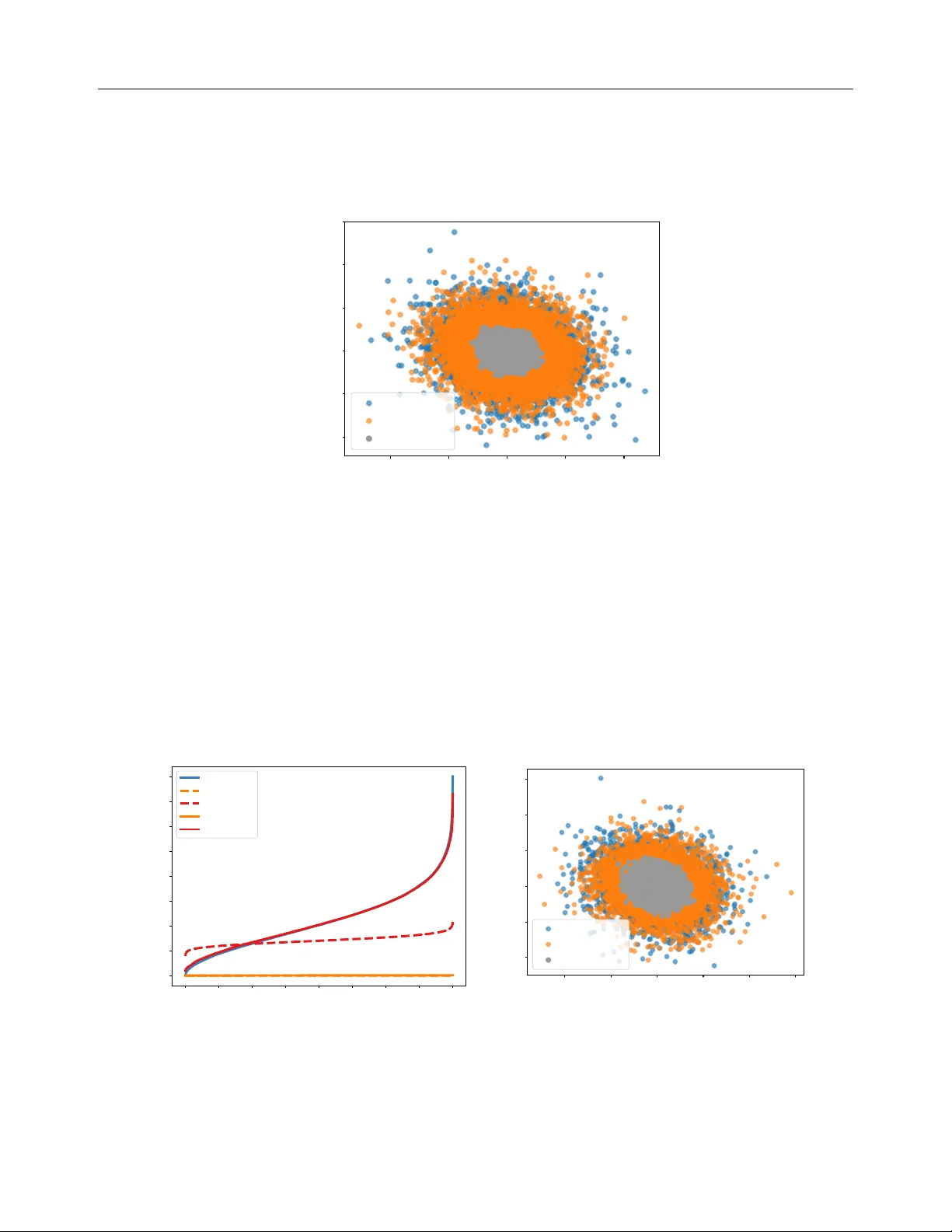
V ariational inference via radial transp ort Luca Ghafourp our 1 , 2 Sinho Chewi 3 Alessio Figalli 1 Aram-Alexandre P o oladian 3 1 ETH Z ¨ uric h 2 Cam bridge 3 Y ale Univ ersity ldg34@cam.ac.uk afigalli@ethz.ch { sinho.chewi,aram-alexandre.pooladian } @yale.edu Abstract In v ariational inference (VI), the practitioner appro ximates a high-dimensional distribution π with a simple surrogate one, often a (pro d- uct) Gaussian distribution. Ho wev er, in many cases of practical interest, Gaussian distri- butions migh t not capture the correct radial profile of π , resulting in p o or cov erage. In this w ork, we approac h the VI problem from the p erspective of optimizing o v er these ra- dial profiles. Our algorithm radVI is a cheap, effectiv e add-on to man y existing VI sc hemes, suc h as Gaussian (mean-field) VI and Laplace appro ximation. W e provide theoretical con- v ergence guarantees for our algorithm, o wing to recen t dev elopmen ts in optimization o v er the W asserstein space —the space of proba- bilit y distributions endow ed with the W asser- stein distance—and new regularit y prop erties of radial transp ort maps in the st yle of Caf- farelli ( 2000 ). 1 In tro duction V ariational inference (VI) is a fundamental optimiza- tion problem that tak es place ov er subsets of probability distributions ( W ainwrigh t and Jordan , 2008 ; Blei et al. , 2017 ). W e consider a standard setup that arises in man y applications, where the practitioner is giv en a high-dimensional p osterior distribution π ∝ exp ( − V ) and the goal is to solv e π ⋆ C : = arg min µ ∈C KL( µ ∥ π ) , Pro ceedings of the 29 th In ternational Conference on Arti- ficial In telligence and Statistics (AIST A TS) 2026, T angier, Moro cco. PMLR: V olume 300. Copyrigh t 2026 b y the au- thor(s). Correspondence to LG and AAP . where C ⊂ P ( R d ) is a fixed set of probability distri- butions. VI is a p o werful computational stand-in for standard Mark ov Chain Mon te Carlo (MCMC) meth- o ds for sampling from unnormalized p osteriors π . In- deed, while MCMC metho ds require sim ulating Marko v c hains for prohibitiv ely long p erio ds of time, it might b e p ossible to instead quickly learn a surrogate density that is a go o d enough approximation to the p osterior for practical purp oses; see the review by Blei et al. ( 2017 ) for more details. In VI, the choice of C ⊂ P ( R d ) is of the utmost imp or- tance. F or example, the case where C is the set of all Gaussians (with p ositiv e definite cov ariance) is known as Gaussian VI ( Barb er and Bishop , 1997 ; Seeger , 1999 ; Opp er and Archam b eau , 2009 ). In large-scale mac hine learning applications, it is also common to optimize o ver the class of Gaussians with diagonal cov ariance, resulting in mean-field Gaussian VI. While these al- gorithms hav e a long history , a rigorous, theoretical analysis is only just emerging, based on the theory of optimal transp ort through W asserstein gradient flo ws ( Am brosio et al. , 2008 ). F or example, the Gaussian case has b een studied by Lambert et al. ( 2022 ); Diao et al. ( 2023 ); Kim et al. ( 2024 ). W e note that it is p ossible to implemen t algorithms based on mixtures of Gaussians as outlined by Lambert et al. ( 2022 ); P etit-T alamon et al. ( 2025 ), though the mathematical analysis in this case is significantly more challenging. Separately , L aplac e approxi mation is an alternativ e means of obtaining a surrogate measure to π , where one considers the following Gaussian approximation N ( x ⋆ , ( ∇ 2 V ( x ⋆ )) − 1 ) where x ⋆ = argmin V . The litera- ture on Laplace approximations is v ast; see e.g., Rob ert and Casella ( 2004 ). Margossian and Saul ( 2025 ) highlight the strengths and weaknesses of existing VI-based algorithms. No- tably , they provide some characterizations for when VI can hop e to exactly reco ver the mean and correlation matrix of a target distribution π . While they are only in terested in these particular statistics, a key detail of the pap er is that the v ariational approximating family V ariational inference via radial transport m ust b e decided in adv ance, which leads to demonstra- ble shortcomings ev en in small-scale examples. 1.1 Con tributions T o mitigate the issues brough t ab out by these appro xi- mations, w e study the VI problem ov er r adial pr ofiles . F or fixed m ∈ R d and Σ ≻ 0, we consider the following v ariational family: p h ( x ) ∝ det(Σ) − 1 / 2 h (( x − m ) ⊤ Σ − 1 ( x − m )) , as h ranges ov er non-negative functions on [0 , ∞ ). If m and Σ are kno wn, or if estimates thereof can b e imputed, then we can assume m = 0 and Σ = I via a whitening pro cedure (see Section 4.5 ). W e henceforth assume that this has b een done, so that our v ariational family is the set C rad of r adial ly symmetric distributions. This family encompasses the standard Gaussian via h ( y ) = exp ( − y / 2), but also Student- t distributions, the non- smo oth Laplace distribution, the logistic distribution, among others. ∗ In this pap er, we prop ose and analyze a tractable algo- rithm for solving π ⋆ rad : = arg min µ ∈C rad KL( µ ∥ π ) , where π ∝ exp ( − V ). Our contributions are of b oth theoretical and computational interest. W e stress that our only assumptions throughout this work will b e on the true p osterior π , namely that π is log-smo oth and strongly log-concav e and centered at the origin. This pair of assumptions has been leveraged in nearly all w orks on the theory of sampling ( Chewi , 2026 ) and in the theoretical and computational study of v ariational inference ( Lambert et al. , 2022 ; Arnese and Lack er , 2024 ; Lac ker et al. , 2024 ; Lav enan t and Zanella , 2024 ; Jiang et al. , 2025 ). In Section 3 , we pro ve existence and uniqueness of the radial minimizer π ⋆ rad , as well as establish regu- larit y prop erties of said minimizer. F or example, if π is log-smo oth and strongly log-concav e, Theorem 3.4 states that π ⋆ rad is as w ell. W e also prov e Caffarelli- t yp e contraction estimates ( Caffarelli , 2000 ) for the corresp onding optimal radial transp ort map T ⋆ rad from the standard Gaussian ρ = N (0 , I ), sa y , to π ⋆ rad ; see Theorem 3.5 . In Section 4 , we embrace the con ven tional wisdom of “parametrizing then optimizing” in order to compute π ⋆ rad , leading to our prop osed algorithm radVI (see ∗ On the other hand, if we fix h and v ary ( m, Σ), w e end up at the theory of elliptical families, see e.g., Muirhead ( 1982 , Section 1.4). Algorithm 1 ). Concretely , w e make use of the repre- sen tation of a giv en radial measure as the pushforw ard of the standard Gaussian b y a radial map T rad . Our approac h is based on carefully parametrizing radial transp ort maps T λ for λ ∈ R J +1 + for some J > 0 where, if J is large enough, our parameterized set should en- compass all p ossible radial maps (see Theorem 4.1 ). Then, writing our ob jectiv e ov er the non-negative or- than t as λ 7→ F ( λ ) = KL(( T λ ) ♯ ρ ∥ π ) ( λ ∈ R J +1 + ) w e sho w that standard Euclidean gradient descent con- v erges to the true optimal radial transp ort map T ⋆ rad , i.e., ∥ T λ ( k ) − T ⋆ rad ∥ L 2 ( ρ ) ≤ ε for all k ≥ e Ω ( ε − 1 ) up to p olynomial factors of the condition n umber of π —see Theorem 4.3 . Notably , our conv ergence guarantees are effectiv ely dimension-fr e e . In Section 5 , we sho w ho w radVI can be (easily) used to impro v e existing VI metho ds on a collection of syn thetic examples. In addition to reco v ering isotropic profiles, w e also sho w ho w radVI can b e used as a preconditioner: giv en any metho d of obtaining a mean-cov ariance pro xy , suc h as through Laplace appro ximation or Gaussian VI, w e sho w how radVI can often impro v e up on the existing appro ximation by b etter capturing the tail b ehavior of the p osterior. As a final example, w e turn to parameter estimation problems (estimating the second momen t, or probabilit y thresholds) giv en an unnormalized posterior. F o cusing on the Neal’s funnel distribution, we sho w ho w radVI on top of full-rank Gaussian VI can lead to substantially improv ed estimates of these quan tities at virtually no added computational cost. W e b eliev e these findings merit further in vestigation. Notation W e write µ ∈ P ( R d ) if µ is a probability measure ov er R d ; µ ∈ P 2 ( R d ) if µ has finite second momen t; µ ∈ P ac ( R d ) if µ has a Leb esgue density; and P 2 , ac ( R d ) = P ac ( R d ) ∩ P 2 ( R d ). F or p ositiv e constants a and b , we write a ≲ b or a = O ( b ) (resp. a ≳ b or a = Ω( b )) to mean there exists a positive constant C suc h that a ≤ C b (resp. a ≥ C b ). If both a ≲ b and b ≲ a , w e write a ≍ b . When omitting logarithmic factors in b , w e write, e.g., a ≲ log b or a = e O ( b ) (analogously for lo wer b ounds). Throughout, implied constants will alw ays b e indep enden t of the dimension and other relev ant problem parameters. W e write the uniform distribution on the unit sphere (denoted S d − 1 ) in R d as Unif . Recall that a function f : R d → R is M -smo oth and m -strongly con vex if 0 ⪯ mI ⪯ ∇ 2 f ⪯ M I . Luca Ghafourp our 1 , 2 Sinho Chewi 3 Alessio Figalli 1 Aram-Alexandre Pooladian 3 2 Bac kground 2.1 Primer on optimal transp ort F or µ, ν ∈ P 2 ( R d ), the squared 2 -Wasserstein distanc e b et ween them is defined as W 2 2 ( µ, ν ) : = inf π ∈ Π( µ,ν ) Z Z ∥ x − y ∥ 2 d π ( x, y ) , (1) where Π( µ, ν ) is the set of joint measures with first marginal µ and second marginal equal to ν . F or more details, see Villani ( 2009 ); Santam brogio ( 2015 ); Chewi et al. ( 2025 ). The asso ciated optimal tr ansp ort map b et ween µ and ν is given by T ⋆ : = arg min T ∈T ( µ,ν ) Z ∥ x − T ( x ) ∥ 2 d µ ( x ) , (2) where T ( µ, ν ) is the set of admissible transp ort maps b et ween µ and ν , which consist of vector-v alued func- tions T : R d → R d suc h that for X ∼ µ , it holds that T ( X ) ∼ ν . Without further assumptions, it is p ossi- ble that such a T ⋆ need not exist. A theorem due to Brenier ( 1991 ) unifies b oth ( 1 ) and ( 2 ). Theorem 2.1 (Brenier’s theorem) . Supp ose µ ∈ P 2 , ac ( R d ) . Then ( 2 ) has a unique minimizer, with W 2 2 ( µ, ν ) = Z ∥ x − T ⋆ ( x ) ∥ 2 d µ ( x ) , and T ⋆ = ∇ φ ⋆ for some c onvex function φ ⋆ . 2.2 Geo desic con v exit y via compatible families of optimal transp ort maps W e no w consider the space of probability measures with densities endo wed with the 2-W asserstein distance, called the Wasserstein sp ac e W 2 : = ( P 2 , ac ( R d ) , W 2 ). Our goal is to formulate the VI problem as an opti- mization problem o ver this space. W e let T rad denote the set of radial (transp ort) maps, whic h are vector-v alued functions T rad : R d → R d with x 7→ T rad ( x ) = Ψ( ∥ x ∥ ) x/ ∥ x ∥ , (3) where Ψ : [0 , ∞ ) → [0 , ∞ ) is strictly monotone and con tin uous. One can c heck that T rad forms a compatible family of optimal transp ort maps (see P anaretos and Zemel , 2020 , Section 2.3.2), and thus ( T rad ) ♯ ρ forms a geo desically conv ex subset of the W asserstein space. F or an in tro duction to the space W 2 fo cused on appli- cations to statistics, see Panaretos and Zemel ( 2020 ); Chewi et al. ( 2025 ). 3 Setup and theoretical results Giv en a p osterior π ∝ exp ( − V ), our ob jectiv e is to compute the follo wing minimizer: π rad ∈ arg min µ ∈C rad KL( µ ∥ π ) , ( radVI ) where we recall that C rad is the set of radially symmet- ric measures. In this section, we first pro ve v arious theoretical properties surrounding π rad , and w e dev elop computational mec hanisms in Section 4 . T o this end, our sole assumption will b e on the true p osterior π ∝ exp ( − V ). Namely , we will assume that π is wel l-c onditione d : it is log-smooth and strongly log-conca ve, i.e., for ℓ V , L V > 0 , 0 ⪯ ℓ V I ⪯ ∇ 2 V ⪯ L V I , ( W C ) and minimized at the origin. These conditions are standard in the theoretical literature on log-concav e sampling ( Chewi , 2026 ) as well as in v ariational infer- ence (see, e.g., Lam b ert et al. , 2022 ; Arnese and Lack er , 2024 ; Lac ker et al. , 2024 ; Lav enan t and Zanella , 2024 ; Jiang et al. , 2025 ). R emark 3.1 . W e note that the smoothness of V is not a particularly strong assumption as, e.g., Gaus- sian mixtures fall in to this class. Ho wev er, the strong con vexit y of V implies unimo dalit y of the posterior, whic h is admittedly stringent. Despite the VI prob- lem b eing well-posed even without this assumption (Prop osition 3.2 ), we require it later in order to obtain guaran tees for our W asserstein gradient flow algorithm. 3.1 Regularit y of radial minimizer W e first collect some basic prop erties of the optimal radial minimizer π ⋆ rad . Proofs of results from this sub- section can b e found in App endix A . W e first state a result concerning the existence and uniqueness of the minimizer π ⋆ rad . Prop osition 3.2. Assume that ther e exists µ ∈ C rad with KL ( µ ∥ π ) < ∞ . Then, ther e exists a unique minimizer to ( radVI ) . Next, we explicitly characterize the stationary condi- tion of the minimizer π ⋆ rad , where the pro of is based on calculus of v ariations. Prop osition 3.3 (Stationary condition) . Supp ose π ∝ exp ( − V ) and a minimizer π ⋆ rad to ( radVI ) exists. Then it holds that π ⋆ rad ∝ exp( − V ) with V ( x ) : = Z S d − 1 V ( ∥ x ∥ θ ) d Unif ( θ ) , (4) wher e Unif is the uniform me asur e on S d − 1 . V ariational inference via radial transport Using Prop osition 3.3 , w e can leverage the existing regularit y of π (through V ) to show that π ⋆ rad is also regular. In particular, log-smo othness and strong log- conca vity are preserved. Prop osition 3.4 (Regularit y of radial minimizer) . Supp ose π satisfies ( W C ) . The r adial minimizer π ⋆ rad also satisfies ( WC ) with the same p ar ameters. 3.2 Regularit y of optimal radial maps W e no w establish regularit y prop erties of optimal radial (transp ort) maps from, say , the standard Gaussian to the minimizer of ( radVI ) . Our main theorem b elo w is essen tially a sp ecialization of Caffarelli’s contraction theorem ( Caffarelli , 2000 ) to the radial comp onen t of the optimal transp ort map. Theorem 3.5 (Regularity of the optimal radial map) . Supp ose π satisfies ( W C ) and c onsider the c orr esp ond- ing minimizer to ( radVI ) , denote d π ⋆ rad . L et T ⋆ rad denote the unique optimal tr ansp ort map fr om ρ to π ⋆ rad , and write T ⋆ rad ( x ) = Ψ ⋆ ( ∥ x ∥ ) x/ ∥ x ∥ . Writing r = ∥ x ∥ , the fol lowing r e gularity c onditions hold: 1 √ L V ≤ (Ψ ⋆ ) ′ ( r ) ≤ 1 √ ℓ V , | (Ψ ⋆ ) ′′ ( r ) | ≲ κ √ ℓ V  1 + d r 2  (1 + | r − √ d | ) , wher e κ : = L V /ℓ V . The first result in Theorem 3.5 follo ws from a direct application of Caffarelli’s contraction theorem; this is made p ossible by Prop osition 3.4 . T o pro ve the sec ond result, w e differen tiate the Monge–Amp` ere equation, and exploit the existing regularity of (the first deriv a- tiv e of ) Ψ ⋆ . A key takea wa y is that under ρ , the norm is tightly concen trated around r = √ d ± O (1), and thus the bound on (Ψ ⋆ ) ′′ is nearly dimension-free. While it is p ossible to differen tiate the Monge–Amp` ere equa- tion a second time and obtain thir d -order control on Ψ ⋆ , w e omit this result as it is not necessary for our purp oses. The full proof of Theorem 3.5 can b e found in App endix B . 4 P arametrize then optimize Recall that our goal is to learn the probability dis- tribution π ⋆ rad giv en query access to the (gradient of the) p oten tial V of the unnormalized p osterior π . Our prop osed algorithm will directly learn the optimal trans- p ort map from ρ (an easy-to-sample reference measure) to the optimal radial distribution π ⋆ rad . W e first note the follo wing equiv alent optimization problems: min µ ∈C rad KL( µ ∥ π ) = min T ∈T rad KL( T ♯ ρ ∥ π ) , where ρ = N (0 , I ). Indeed, an y radial distribution µ ∈ C rad can be expressed as the pushforward of the standard Gaussian with an y other radial transport map in T rad . Thus, in this section, we will b e fo cusing on the optimization problem T ⋆ rad = arg min T ∈T rad KL( T ♯ ρ ∥ π ) , ( radVI - T ) from whic h we recov er the optimal radial distribution. W e follow the approac h put forth by Jiang et al. ( 2025 ), who suggest to appropriately p ar ametrize the space of transp ort maps and then to optimize ov er it. Letting { Ψ j } J j =0 b e a fixed set of basis fun ctions and α > 0, w e consider a parametrized subset of transp ort maps T J ⊆ T rad , giv en by T J : = n α ∥ x ∥ + J X j =0 λ j Ψ j ( ∥ x ∥ )  x ∥ x ∥    λ ∈ R J +1 + o . (5) In the rest of this section, we will address the following questions, whic h naturally arise as a result of our c hoice of parametrization: • What is the prop osed basis { Ψ j } J j =0 ? Ho w large do es J need to be such that T J is a faithful ap- pro ximation to T rad ? • Do es optimizing ov er T J yield a map which is close to T ⋆ rad ? Is it p ossible to obtain optimization guaran tees? 4.1 Appro ximation guarantees W e first describ e our choice of basis. As an arbitrary function Ψ is a contin uous, strictly monotone function, w e parametrize this class of functions by a piecewise linear monotone curv e. Given a cutoff v ariable R > 0, w e consider the following sequence of equi-spaced piecewise monotone functions on the interv al [ √ d − R, √ d + R ] ⊂ R Ψ j ( r ) : = Ψ base ( δ − 1 j ( r − a j )) , (6) where for j ≥ 1, δ j : = δ is the mesh size, { a j } J j =1 are the knots; and for j = 0, δ 0 : = √ d − R and a 0 : = 0. Here, Ψ base ( x ) : = 0 ∨ ( x ∧ 1). Ultimately , w e will choose J = 2 R/δ + 1 (we assume that R is divisible by δ and that R ≤ √ d ). Our first result of this section establishes a “univer- salit y” prop ert y of the set T J from an approximation Luca Ghafourp our 1 , 2 Sinho Chewi 3 Alessio Figalli 1 Aram-Alexandre Pooladian 3 p erspective, and yields the choice of R and J required to complete our construction. Theorem 4.1 (Univ ersal approximation) . L et T ⋆ ∈ T rad which satisfies The or em 3.5 , and let ε ≫ exp( − Ω( d )) . Define T J with α = 1 / √ L V and cho ose R ≍ p log( d/ε ) , J = e Ω( p κ/ε ) with the b asis elements given by ( 6 ) . Then ther e exists a ˆ T ∈ T J , i.e., ther e exists ˆ λ ∈ R J +1 + with ˆ T = T ˆ λ , such that ∥ T ⋆ − ˆ T ∥ L 2 ( ρ ) ≤ ε/ℓ 1 / 2 V , ∥ D ( T ⋆ − ˆ T ) ∥ L 2 ( ρ ) ≤ e O ( κ 1 / 2 ε 1 / 2 /ℓ 1 / 2 V ) . 4.2 Prop osed algorithm: radVI W e now present our basic algorithm. Recall that our ob jective function, the KL divergence, is KL( µ ∥ π ) = V ( µ ) + H ( µ ) + log Z , : = Z V d µ + Z log µ d µ + log Z , where Z > 0 is the unknown normalizing constan t of π . If we write µ = T ♯ ρ , for some transp ort map T , then b y a change-of-v ariables calculation, one obtains (up to omitted constan ts) KL( T ♯ ρ ∥ π ) = Z V ◦ T d ρ − Z log det D T d ρ . W e no w optimize ov er our prescrib ed parametrization. F or T λ ∈ T J , w e see that w e can write the KL div er- gence as a function o ver the non-negative orthant: λ 7→ F ( T λ ) : = KL(( T λ ) ♯ρ ∥ π ) ( λ ∈ R J +1 + ) . (7) T o con tinue, w e require the follo wing observ ation: there exists an isometry b et ween the L 2 ( ρ ) distance on the transp ort maps T λ ∈ T J and a Euclidean distance o ver the weigh ts λ ∈ R J +1 + . Indeed, for any tw o parameters λ, η ∈ R J +1 + , one readily computes ∥ T λ − T η ∥ 2 L 2 ( ρ ) = ∥ P J j =1 ( λ j − η j ) Ψ j ( ∥ x ∥ ) ∥ 2 L 2 ( ρ ) = ( λ − η ) ⊤ Q ( λ − η ) , where Q ∈ S J +1 + is a Gram matrix with entries giv en by Q i,j : = E X ∼ ρ [Ψ i ( ∥ X ∥ ) Ψ j ( ∥ X ∥ )] . W e detail in App endix C.2 ho w to compute the en tries Q i,j via truncated moments of the chi distribution. Th us, con vergence of the radial maps corresp onds to conv ergence of the parameters in a weighte d Euclidean space, namely ( R J +1 + , ∥ · ∥ Q ). In other w ords, a discretization of a gradient flow of ( 7 ) w ould Algorithm 1 radVI Input: P osterior π ∝ exp( − V ) with access to ∇ V F ree parameters: Cho ose K, h > 0 Construct: Basis family { Ψ j } J j =0 and matrix Q Initialize: λ (0) ∈ R J +1 + while k = 0 , 1 , . . . , K − 1 do Compute sto c hastic gradient b ∇ λ F ( T λ ( k ) ) λ ( k +1) = Pro j R J +1 + , ∥·∥ Q  λ ( k ) − hQ − 1 b ∇ λ F ( T λ ( k ) )  end while Return: T λ ( K ) naturally corresp ond to pr oje cte d gr adient desc ent in the w eighted metric ∥ · ∥ Q : λ ( k +1) = Pro j R J +1 + , ∥·∥ Q  λ ( k ) − hQ − 1 ∇ λ F ( T λ ( k ) )  , (8) where h > 0 is the stepsize, and ∇ λ F ( T λ ) is the gradien t of the ob jective function in the parameters λ . Our complete algorithm, called radVI , is presen ted in Algorithm 1 . Note that in practice, a stochastic estimate of the gradient will b e used in place of the full gradien t. Thus, radVI can b e seen as a sp ecial instance of sto chastic pro jected gradient descen t (SPGD). W e discuss this more in Section 4.4 . R emark 4.2 . It is worth stressing that the choice of using gradien t descent as a first-order algorithm w as en- tirely arbitrary , and man y other algorithms (e.g., F rank– W olfe, mirror descent, etc.) are applicable within our framew ork. The functional of interest can b e suitably arbitrary as well; see Jiang et al. ( 2025 ) for more details. 4.3 Optimization guaran tees The main result of this section is the follo wing quanti- tativ e conv ergence of radVI to the optimal radial map. Theorem 4.3 (Con vergence of radVI ) . Supp ose π satisfies ( W C ) , and c onsider the family of tr ansp ort maps c onstructe d via ( 6 ) . Then, the tr ansp ort map T λ ( K ) with ( λ ( k ) ) k ≥ 0 given by ( 8 ) is ε -close to T ⋆ rad (in L 2 ( ρ ) ) so long as J = e Θ ( κ 2 /ε ) , the step size h = e Θ( ε/ ( L V κ 2 )) and for iter ations K = e Ω  κ 5 ε − 1 log(KL(( T λ (0) ) ♯ ρ ∥ π ) /ε 2 )  . W e outline a pro of sketc h, lea ving the fine details to App endix C.4 . Let us first assume that the sequence ( λ ( k ) ) k ≥ 0 ev entually conv erges to some optimal λ ⋆ ∈ R J +1 + . If π satisfies ( W C ) , then the corresp onding T ⋆ rad satisfies the Theorem 3.5 . Also, b y Theorem 4.1 , there V ariational inference via radial transport exists ˆ λ ∈ R J +1 + suc h that T ˆ λ ∈ T J is ε -close to T ⋆ rad for J sufficien tly large. By triangle inequality , w e hav e ∥ T λ ⋆ − T ⋆ rad ∥ 2 L 2 ( ρ ) ≲ ∥ T λ ⋆ − T ˆ λ ∥ 2 L 2 ( ρ ) + ∥ T ˆ λ − T ⋆ rad ∥ 2 L 2 ( ρ ) ≲ ∥ T λ ⋆ − T ˆ λ ∥ 2 L 2 ( ρ ) + ε 2 . App ealing to the strong conv exity of the KL divergence along generalized geo desics, one can show that the remaining term can be b ounded b y precisely b oth terms from Theorem 3.5 ∥ T λ ⋆ − T ˆ λ ∥ 2 L 2 ( ρ ) ≲ κ ∥ T ˆ λ − T ⋆ rad ∥ 2 L 2 ( ρ ) + κ 2 ∥ D ( T ˆ λ − T ⋆ rad ) ∥ 2 L 2 ( ρ ) . (9) See Jiang et al. ( 2025 , App endix C) for a pro of of this fact (in particular, the pro of of their Theorem 5.9 and Corollary C.3). Thus, for J large enough, the mini- mizer o ver T J , i.e., T λ ⋆ , can be made arbitrarily close to T ⋆ rad . T o conclude, it remains to quantitativ ely assess that T λ ( k ) → T λ ⋆ , and then string everything together. By the isometry prop ert y , it holds that ∥ T λ ( k ) − T λ ⋆ ∥ 2 L 2 ( ρ ) = ∥ λ ( k ) − λ ⋆ ∥ 2 Q , where w e recall that Q ≻ 0 is the fixed Gram matrix de- fined from the basis functions. If λ 7→ F ( T λ ) is smo oth and strongly conv ex (with resp ect to ∥ · ∥ Q ), w e can readily apply existing results for the conv ergence of first-order algorithms (see, e.g., Beck , 2017 ). Thank- fully , the requisite prop erties of our functional can b e v erified; see App endix C.3 . Prop osition 4.4. Supp ose π satisfies ( W C ) , and also c onsider T J chosen as in The or em 4.1 . Then λ 7→ F ( T λ ) is ℓ V -str ongly c onvex and e O ( J 2 L V ) -smo oth (with r esp e ct to ∥ · ∥ Q ). R emark 4.5 . Note that the smo othness constant of λ 7→ F ( T λ ) explo des as J → ∞ . This is unsurprising, as the functional µ 7→ KL ( µ ∥ π ) is not smo oth o ver the space of all probability measures. In contrast, our parametrization creates a strict subset of all probabilit y measures, o ver which the constant can b e controlled. 4.4 Sto c hastic optimization In practice, w e use sto chastic pro jected gradien t descent (SPGD) to optimize λ 7→ F ( T λ ) ov er ( R J +1 + , ∥ · ∥ Q ). Recall our full ob jective function (up to constants) is F ( T λ ) = Z V ( T λ ( x )) d ρ ( x ) − Z log det( D T λ ( x )) d ρ ( x ) . W e compute the gradient of the tw o terms separately . F or the first term, we pass the gradient in the weigh ts λ under the exp ectation and, due to the definition of T λ , the inner gradien t is simply ∇ λ V ( T λ ( X )) =  Ψ( ∥ X ∥ )( X/ ∥ X ∥ ) ⊤ ∇ V ( T λ ( X )) , (10) where  Ψ ( r ) : = [Ψ 0 ( r ) , . . . , Ψ J ( r )]. Thus, to compute ∇ λ E X ∼ ρ [ V ( T λ ( X ))], it suffices to use a Monte Carlo appro ximation using i.i.d. draws X 1 , . . . , X N ∼ ρ . F or the second term, w e first compute log det( D T λ ( x )) = ( d − 1) log( α + ⟨ λ,  Ψ( ∥ x ∥ ) ⟩ / ∥ x ∥ ) + log( α + ⟨ λ,  Ψ ′ ( ∥ x ∥ ) ⟩ ) , where  Ψ ′ ( r ) : = [Ψ ′ 0 ( r ) , . . . , Ψ ′ J ( r )]. It is straightforw ard to show that ∇ λ log det ( D T λ ( x )) has an analytical ex- pression, and thus the integrated expression can again b e computed via Mon te Carlo integration. How ever, due to the precise nature of  Ψ and  Ψ ′ , it is p ossible to ev aluate our second integrated quan tity in our ob jec- tiv e using simple univ ariate numerical integration; we briefly touc h on this in App endix C.5 . The next theorem states that radVI still comes with con v ergence guarantees when using stochastic gradient estimates (e.g., Monte Carlo estimates) for ( 10 ) . Un- lik e many works that use SPGD, we pr ove that under the w ell-conditioned assumption, we satisfy a classical b ounde d varianc e prop erty which p ermits us to use existing theory; see App endix C.6 for a pro of. Theorem 4.6 (Conv ergence of sto c hastic radVI ) . As- sume that π is wel l-c onditione d W C and c onsider the family of tr ansp ort maps c onstructe d via ( 6 ) . Then, for al l sufficiently smal l ε , the iter ates of sto chastic pr oje cte d gr adient desc ent yield a me asur e µ ( t ) with the guar ante e ℓ V E ∥ T λ ( k ) − T ⋆ rad ∥ 2 L 2 ( ρ ) ≤ ε 2 , with a numb er of iter ations b ounde d by K = e Ω  dκ 2 J 3 L V ε − 2 log( ∥ T λ (0) − T ⋆ rad ∥ 2 L 2 ( ρ ) /ε )  , and step size h = e Θ ( ε 2 / ( dκ 3 J 3 L V )) . Mor e over, if we cho ose the p ar ameters of our dictionary as in The o- r em 4.1 , then we achieve the same ε -closeness ab ove with K = e Ω  dκ 5 / 2 ε − 5 log( ∥ T λ (0) − T ⋆ rad ∥ 2 L 2 ( ρ ) /ε )  . 4.5 radVI with whitening As we highligh ted in the introduction, a strength of radVI is that it can b e used in conjunction with other v ariational metho ds based on, say , Gaussian distribu- tions, such as Gaussian VI, mean-field Gaussian VI, and Laplace approximation. Algorithm 2 illustrates ho w to use any of these off-the-shelf Gaussian approxi- mation metho ds to whiten the target distribution and impro ve p erformance. Luca Ghafourp our 1 , 2 Sinho Chewi 3 Alessio Figalli 1 Aram-Alexandre Pooladian 3 Algorithm 2 radVI with whitening Input: P osterior π ∝ exp( − V ) with access to ∇ V Whitening stage: 1. Fix ( m, Σ) ∈ R d × S d + 2. Define x 7→ T m, Σ ( x ) : = Σ 1 / 2 x + m 3. Mo dify p osterior via e V ← V ◦ T m, Σ Obtain: ˆ T rad ← radVI (exp( − e V )) Return: Composite map T comp ← T m, Σ ◦ ˆ T rad In summary , any Gaussian measure N ( m, Σ) can b e expressed as ( T m, Σ ) ♯ ρ where ρ = N (0 , I ) and T m, Σ ( x ) = Σ 1 / 2 x + m . Thus, given any Gaussian ap- pro ximation to π , w e can use the corresp onding affine map to whiten the p osterior π ∝ exp ( − V ) by defining e V : = V ◦ T m, Σ . Then, we run radVI on exp ( − e V ), and output the comp osition of these tw o maps. Below, we briefly review t wo standard Gaussian approximation metho ds in the literature. Laplace appro ximations (LA). The Laplace ap- pro ximation metho d o ccurs in tw o stages. F or a p os- terior π ∝ exp ( − V ), we first compute the mo de of the distribution, x ⋆ ∈ arg min x ∈ R d V ( x ), and then we compute ( ∇ 2 V ( x ⋆ )) − 1 . The final approximation to the p osterior π is then π LA = N ( x ⋆ , ( ∇ 2 V ( x ⋆ )) − 1 ) . (11) Note that this metho d fails if ∇ 2 V ( x ⋆ ) is not in v ertible, and is kno wn to b e inaccurate when π is hea vily sk ew ed (when the mo de is far aw ay from the mean). See Kat- sevic h ( 2023 , 2024 ) for recent statistical developmen ts. Gaussian VI (GVI). In Gaussian VI, the practi- tioner replaces C rad in ( radVI ) with N , the set of all normal distributions with p ositive definite co v ariance. The resulting optimization problem b ecomes π GVI ∈ arg min µ ∈N KL( µ ∥ π ) ; (12) see Lambert et al. ( 2022 ); Diao et al. ( 2023 ); Kim et al. ( 2023 ). A ma jor limitation to GVI is the storage and p er-iteration complexit y , as the running cov ariance esti- mate needs to b e stored and inv erted at each iteration, whic h is costly for d ≫ 1. Optimizing o ver pr o duct Gaussian measures (Gaussian mean-field VI, or MFVI) can mitigate these numerical hurdles, reducing the p er- iteration complexit y from O ( d 3 ) to O ( d ) at the cost of p ossibly b eing muc h farther from π . R emark 4.7 . W e briefly mention the work of Liang et al. ( 2022 ), which similarly tries to adjust the tail distributions of their approximated distribution. How- ev er, their approach is (i) parametric in nature, and (ii) 0 2500 5000 7500 10000 10 − 3 10 − 2 10 − 1 10 0 10 1 10 2 10 3 W 2 2 distance Gaussian target Laplace target Logistic target Student-t target Figure 1: Conv ergence of radVI for v arious target distributions. See T able 1 for final-iterate comparisons b et ween GVI and LA. builds off the mean-field v ariational inference p ersp ec- tiv e. Specifically , they only consider pro duct measure appro ximations to the p osteriors. 5 Exp erimen ts In all exp erimen ts, d = 50, w e choose α = 0 . 01 and λ (0) = 1 J , R = √ log d , and δ = d − 1 / 6 as parameters for constructing our dictionary . F or LA, w e use a stan- dard optimization solver and closed-form expressions of the gradient and Hessian. F or GVI, w e use the F orw ard–Backw ard metho d of Diao et al. ( 2023 ). † The candidate p osteriors for the ma jority of this section are the Student- t , Laplace, and logistic distributions. W e remark that none of these distributions fully sat- isfy our requirements. F or instance, none of them are strongly conv ex (in fact, the Student- t distribution is non-log-concav e), and the Laplace distribution is non-smo oth. F or Student- t , w e use 10 degrees of free- dom, which leads to significantly heavier tails than a Gaussian. Nev ertheless, w e are able to sho w that our sc heme can recov er the desired target distribution to b etter accuracy than standard VI metho ds. The precise definitions of these distributions, their p oten tial functions, etc., can b e found in Appendix D.2 . In Sec- tion 5.3 , we study parameter estimation from Neal’s funnel distribution, a standard hierarc hical prior. 5.1 Learning isotropic radial families W e first inv estigate the case where the target measure is isotropic and radially symmetric. As π = π ⋆ rad = ( T ⋆ rad ) ♯ ρ , for any iterate λ ( k ) in our algorithm, we can † The co de used for our implemen tation of radVI and the n umerical experiments are made a v ailable at gith ub.com/gluca99/radVI . V ariational inference via radial transport Isotropic targets Method Gaussian Laplace Logistic Studen t- t LA 2 . 45 × 10 − 4 20 . 00 1 . 6 × 10 3 25 . 87 GVI 7 . 34 × 10 − 4 8 . 24 3 . 96 1 . 99 radVI 1 . 15 × 10 − 4 5 . 37 × 10 − 2 1 . 84 × 10 − 1 1 . 19 × 10 − 1 T able 1: Estimated W asserstein distance betw een v ari- ous VI solutions for learning isotropic targets. appro ximate the L 2 distance b et ween the maps via ∥ T λ ( k ) − T ⋆ rad ∥ 2 L 2 ( ρ ) ≃ 1 n n X i =1 ∥ T λ ( k ) ( X i ) − T ⋆ rad ( X i ) ∥ 2 , where X i ∼ ρ , and we use n = 10 4 to estimate all quan- tities. T ⋆ rad is known in closed form for the Gaussian case and Student- t distribution, but must be solved n umerically for the logistic and Laplace distributions; see App endix D.2 for a short explanation. W e compare the (squared) 2-W asserstein distance b et ween ground truth samples and those generated by LA and GVI. See Figure 1 for a plot comparing the conv ergence of these v arious metho ds. As a sanity chec k, our metho d recov- ers the Gaussian distribution with an error tolerance comparable to Gaussian metho ds. F or the heavy-tailed Studen t- t distribution, how ever, we outp erform these metho ds by wide margins. Repeating the exp erimen t in d = 100 giv es similar results (see App endix E.1 ). It is p erhaps more informative to visually distinguish the approximation schemes. T o this end, we plot the radial profiles of the v arious appro ximation metho ds. F or instance, the top of Figure 2 compares the v arious learned profiles for the Student- t distribution. Unlik e LA or GVI, radVI can find a close radial profile to the target. The corresp onding figures for isotropic Laplace and logistic distributions app ear in App endix E . Finally , we mention that we additionally p erformed a simple sensitivity analysis regarding our hyperpa- rameter α similar to Figure 2 of Jiang et al. ( 2025 ). F o cusing on the isotropic Gaussian case in whic h the ground-truth v alue is α = 1 / √ L V = 1, we run our al- gorithm where we v ary α ∈ { 10 0 , 10 − 1 , 10 − 2 } . Figure 3 sho ws that radVI con v erges to the optimal parameters exp onen tially fast, highligh ting how our algorithm is robust to the c hoice of α . 5.2 Learning anisotropic distributions W e now consider the anisotropic setting, where the dis- tribution has a randomly generated co v ariance parame- ter Σ = AA ⊤ + I , where A ij ∼ N (0 , 1) and m = 0. F ol- lo wing Algorithm 2 , w e first run either LA or GVI to cre- ate Gaussian appro ximations, and then we obtain our complete comp osite map, allo wing us to dra w as many 0 2500 5000 7500 10000 12500 15000 17500 20000 Sorted r 5 10 15 20 25 Sorted radial pushforward T arget radVI LA GVI 0 2500 5000 7500 10000 12500 15000 17500 20000 Sorted r 25 50 75 100 125 150 175 Sorted radial pushforward T arget LA GVI LA+ radVI GVI+ radVI Figure 2: Comparing learned radial profiles of radVI v ersus other approximation metho ds for learning the Studen t- t distribution in the isotropic ( top ) and anisotropic case (b ottom) . 0 2000 4000 6000 8000 10000 10 − 3 10 − 2 10 − 1 10 0 10 1 L 2 loss α = 1 α = 0 . 1 α = 0 . 01 Figure 3: In the case where π is an isotropic Gaussian with d = 50, we v erify that radVI is robust to the c hoice of α . samples as desired. Figure 4 show cases performance on an anisotropic logistic where we visualize generated samples. The Gaussian approximation metho ds fail to capture the correct tail b eha vior, while the whitened Luca Ghafourp our 1 , 2 Sinho Chewi 3 Alessio Figalli 1 Aram-Alexandre Pooladian 3 0 2500 5000 7500 10000 12500 15000 17500 20000 Sorted r 100 200 300 400 500 600 Sorted radial pushforward T arget LA GVI LA+ radVI GVI+ radVI − 200 − 100 0 100 200 x 0 − 200 − 100 0 100 200 x 1 T arget LA+ radVI LA Figure 4: T op: Comparing whitening metho ds for learning the anisotropic logistic distribution, with and without radVI . Bottom: Visual comparison of true target samples, those generated b y LA, and ours (LA+ radVI ). radVI appro ximations do. W e observe the same p erfor- mance for the anisotropic Student- t and Laplace distri- butions; see the b ottom of Figure 2 and App endix E . 5.3 radVI for parameter estimation W e now demonstrate how radVI can correct tail- underestimation for certain p osteriors π . T o illustrate this, first let f : R d → R b e a functional of in terest and consider the problem of estimating E X ∼ π [ f ( X )] . Letting b π denote a generic v ariational approximation, note that w e alwa ys hav e the approximation E X ∼ π [ f ( X )] = E Y ∼ b π [ f ( Y ) π ( Y ) / b π ( Y )] ≈ 1 n n X i =1 [ f ( Y i ) π ( Y i ) / b π ( Y i )] , where Y i ∼ b π are easily-drawn samples. T o inv estigate how radVI can b e used to improv e GVI for parameter estimation, w e study Neal’s funnel distri- bution, a common example in the VI literature ( Neal , d = 25 Parameter E [ z 2 ] = 4 E [ x 2 1 ] ≈ 7 . 389 P ( z > 2) ≈ 0 . 51 GVI 0.274 ± 4 × 10 − 3 1.12 ± 1 . 4 × 10 − 2 0 GVI+radVI 2 . 41 ± 2 × 10 − 2 5 . 96 ± 1 . 0 × 10 − 1 0 . 214 ± 3 × 10 − 3 d = 50 Parameter E [ z 2 ] = 4 E [ x 2 1 ] ≈ 7 . 389 P ( z > 2) ≈ 0 . 51 GVI 0.328 ± 5 × 10 − 3 1.61 ± 2 × 10 − 2 0 GVI+radVI 2 . 51 ± 4 × 10 − 2 6 . 48 ± 2 × 10 − 1 0 . 19 ± 5 × 10 − 3 T able 2: In d ∈ { 25 , 50 } , w e compare the p erformance of GVI and GVI+ radVI for parameter estimation; in paren theses we include the effective sample size. 2003 ; Betancourt and Girolami , 2015 ). F or d > 1, sup- p ose z ∼ N (0 , 4) and x i ∼ N (0 , e z ) for i ∈ [ d ]; one can explicitly write π ∈ P ( R d +1 ) and compute the cor- resp onding log-density and its deriv atives. W e stress that this mo del is misspecified for radial distributions, and instead fall under the category of a structur e d p os- terior ( Sheng et al. , 2025 ). W e follow related work and estimate the following quantities from the p osterior: E [ z 2 ] = 4, E [ x 2 1 ] ≈ 7 . 389, and P ( z > 2) ≈ 0 . 51. In T able 2 , we rep ort our results. W e drew 2000 samples from b oth GVI and GVI+ radVI , and rep orted the estimated parameters av eraged ov er 1000 trials and also computed the standard error (av eraged across the trials). As exp ected, the parameter estimates are significan tly b etter when incorp orating radVI , which w e stress comes with minimal computational cost. F or instance, standard Gaussian VI will rep ort that the tail probability is identically zero whereas our estimate using radVI is significan tly closer to the ground truth. 6 Conclusion W e prop ose and analyze a framew ork for v ariational in- ference ov er the space of r adial transp ort maps, leading to our algorithm, radVI . Under standard assumptions, w e pro ve con vergence guaran tees for our algorithm in b oth the deterministic and sto c hastic settings. Our analysis hinges on nov el regularity prop erties of opti- mal transport maps b et w een radially symmetric dis- tributions. W e demonstrate our ability to learn radial distributions in a suite of exp erimen ts where standard VI metho ds fail to capture the correct behavior. An in teresting op en question is to lift the log-concav e as- sumptions and still obtain optimization guaran tees in this setting, as man y hav e in the sampling literature ( Balasubramanian et al. , 2022 ; Chewi , 2026 ). Ac knowledgemen ts AAP thanks the Y ale Institute for the F oundations of Data Science for financial supp ort. V ariational inference via radial transport References Am brosio, L., Gigli, N., and Sav ar´ e, G. (2008). Gr adient flows: in metric sp ac es and in the sp ac e of pr ob ability me asur es . Springer Science & Business Media. Arnese, M. and Lac ker, D. (2024). Con v ergence of co- ordinate ascent v ariational inference for log-concav e measures via optimal transp ort. arXiv pr eprint arXiv:2404.08792 . Balasubramanian, K., Chewi, S., Erdogdu, M. A., Salim, A., and Zhang, S. (2022). T ow ards a theory of non-log-concav e sampling: first-order stationarity guaran tees for Langevin Monte Carlo. In Confer enc e on L e arning The ory , pages 2896–2923. PMLR. Barb er, D. and Bishop, C. (1997). Ensem ble learning for multi-la yer netw orks. In Jordan, M., Kearns, M., and Solla, S., editors, A dvanc es in Neur al Informa- tion Pr o c essing Systems , volume 10. MIT Press. Bec k, A. (2017). First-or der metho ds in optimization . SIAM. Betancourt, M. and Girolami, M. (2015). Hamiltonian Mon te Carlo for hierarchical mo dels. Curr ent tr ends in Bayesian metho dolo gy with applic ations , 79(30):2– 4. Blei, D., Kucukelbir, A., and McAuliffe, J. (2017). V ari- ational inference: a review for statisticians. Journal of the Americ an Statistic al Asso ciation , 112:859–877. Brenier, Y. (1991). P olar factorization and monotone rearrangemen t of v ector-v alued functions. Communi- c ations on Pur e and Applie d Mathematics , 44(4):375– 417. Bren t, R. P . (1973). Some efficient algorithms for solv- ing systems of nonlinear equations. SIAM Journal on Numeric al A nalysis , 10(2):327–344. Caffarelli, L. A. (2000). Monotonicity prop erties of optimal transp ortation and the FK G and related in- equalities. Communic ations in Mathematic al Physics , 214. Chewi, S. (2026). Log-conca ve sampling. Av ailable at https://chewisinho.github.io/ . Chewi, S., Niles-W eed, J., and Rigollet, P . (2025). Sta- tistic al optimal tr ansp ort , v olume 2364 of L e ctur e Notes in Mathematics . Springer, Cham. ´ Ecole d’ ´ Et ´ e de Probabilit ´ es de Sain t-Flour XLIX – 2019. Chewi, S. and P o oladian, A.-A. (2023). An en- tropic generalization of Caffarelli’s contraction the- orem via cov ariance inequalities. Comptes R endus. Math ´ ematique , 361(G9):1471–1482. Diao, M. Z., Balasubramanian, K., Chewi, S., and Salim, A. (2023). F orward-bac kward Gaussian v aria- tional inference via JKO in the Bures–Wasserstein space. In International Confer enc e on Machine L e arning , pages 7960–7991. PMLR. Jiang, Y., Chewi, S., and P o oladian, A.-A. (2025). Algorithms for mean-field v ariational inference via p olyhedral optimization in the Wasserstein space. F oundations of Computational Mathematics , pages 1–52. Katsevic h, A. (2023). The Laplace approximation accu- racy in high dimensions: a refined analysis and new sk ew adjustment. arXiv pr eprint arXiv:2306.07262 . Katsevic h, A. (2024). The Laplace asymptotic expansion in high dimensions. arXiv pr eprint arXiv:2406.12706 . Kim, K., Oh, J., W u, K., Ma, Y., and Gardner, J. (2023). On the con vergence of black-box v ariational inference. A dvanc es in Neur al Information Pr o c ess- ing Systems , 36:44615–44657. Kim, Y., W ang, W., Carb onetto, P ., and Stephens, M. (2024). A flexible empirical Bay es approac h to m ulti- ple linear regression and connections with p enalized regression. Journal of Machine L e arning R ese ar ch , 25(185):1–59. Lac ker, D., Mukherjee, S., and Y eung, L. C. (2024). Mean field approximations via log-concavit y . Inter- national Mathematics R ese ar ch Notic es , 2024:6008– 6042. Lam b ert, M., Chewi, S., Bac h, F., Bonnab el, S., and Rigollet, P . (2022). V ariational inference via W asser- stein gradient flo ws. A dvanc es in Neur al Information Pr o c essing Systems , 35. La venan t, H. and Zanella, G. (2024). Conv ergence rate of random scan co ordinate ascent v ariational inference under log-concavit y . SIAM Journal on Optimization , 34(4):3750–3761. Liang, F., Mahoney , M., and Hodgkinson, L. (2022). F at–tailed v ariational inference with anisotropic tail adaptiv e flows. In International Confer enc e on Ma- chine L e arning , pages 13257–13270. PMLR. Margossian, C. and Saul, L. K. (2025). V ariational inference in lo cation-scale families: exact recov ery of the mean and correlation matrix. In International Confer enc e on Artificial Intel ligenc e and Statistics , pages 3466–3474. PMLR. Muirhead, R. J. (1982). Asp e cts of multivariate statis- tic al the ory . Wiley Series in Probability and Math- ematical Statistics. John Wiley & Sons, Inc., New Y ork. Neal, R. M. (2003). Slice sampling. The Annals of Statistics , 31(3):705–767. Opp er, M. and Arc hambeau, C. (2009). The v ariational Gaussian appro ximation revisited. Neur al Comput. , 21(3):786–792. Luca Ghafourp our 1 , 2 Sinho Chewi 3 Alessio Figalli 1 Aram-Alexandre Pooladian 3 P anaretos, V. M. and Zemel, Y. (2020). An invitation to statistics in Wasserstein sp ac e . Springer Nature. P etit-T alamon, M., Lambert, M., and Korba, A. (2025). V ariational inference with mixtures of isotropic Gaus- sians. In The Thirty-ninth Annual Confer enc e on Neur al Information Pr o c essing Systems . Rob ert, C. and Casella, G. (2004). Monte Carlo statis- tic al metho ds . Springer-V erlag. San tam brogio, F. (2015). Optimal transport for applied mathematicians. Birk¨ auser, NY , 55(58-63):94. Seeger, M. (1999). Ba y esian model selection for supp ort v ector mac hines, Gaussian pro cesses and other k ernel classifiers. In Solla, S., Leen, T., and M ¨ uller, K., editors, A dvanc es in Neur al Information Pr o c essing Systems , v olume 12. MIT Press. Sheng, S., W u, B., Zhu, B., Chewi, S., and P o ola- dian, A.-A. (2025). Theory and computation for structured v ariational inference. arXiv pr eprint arXiv:2511.09897 . V an Handel, R. (2014). Probability in high dimension. L e ctur e notes (Princ eton University) , 2(3):2–3. Villani, C. (2009). Optimal tr ansp ort: old and new , v olume 338. Springer. Virtanen, P ., Gommers, R., Oliphan t, T. E., Hab er- land, M., Reddy , T., Cournap eau, D., Burovski, E., P eterson, P ., W eck esser, W., Bright, J., et al. (2020). SciPy 1.0: fundamental algorithms for scien tific com- puting in Python. Natur e Metho ds , 17(3):261–272. W ain wright, M. J. and Jordan, M. I. (2008). Graph- ical mo dels, exponential families, and v ariational inference. F oundations and T r ends ® in Machine L e arning , 1:1–305. V ariational inference via radial transp ort A Omitted pro ofs from Section 3.1 A.1 Pro of of Prop osition 3.2 The existence of a minimizer follows from standard argumen ts, since the KL divergence is w eakly low er semicon- tin uous, has (weakly) compact sublevel sets, and C rad is (weakly) closed. Uniqueness follows from strict conv exity of the KL divergence, together with conv exity of C rad : if µ, ν ∈ C rad , then 1 2 ( µ + ν ) ∈ C rad , since a mixture of tw o radial measures is radial. A.2 Pro of of Prop osition 3.3 Recall that KL( µ ∥ π ) = Z V ( y ) d µ ( y ) + Z log( µ ( y )) d µ ( y ) , where µ ∈ C rad . As µ is radial, we can express the ab ov e in p olar co ordinates as s − 1 d KL( µ ∥ π ) = Z ∞ 0 Z S d − 1 V ( r θ ) µ ( r ) r d − 1 d Unif ( θ ) d r + Z ∞ 0 log µ ( r ) µ ( r ) r d − 1 d r , where µ ( r ) : = µ ( r θ ) for some (thus all) θ ∈ S d − 1 , and s d denotes the v olume of S d − 1 . T aking the first v ariation in µ , one computes Z S d − 1 V ( r θ ) d Unif ( θ ) + log µ ( r ) = constan t . Rearranging yields the claim. A.3 Pro of of Prop osition 3.4 W e first require the follo wing computation. Lemma A.1. If V is L V -smo oth and ℓ V -str ongly c onvex, then r 7→ V ( r ) : = R S d − 1 V ( r θ ) d Unif ( θ ) is L V -smo oth and ℓ V -str ongly c onvex. Pr o of. W e compute the first and second deriv ativ es by t wo applications of the chain rule: V ′ ( r ) = d d r Z S d − 1 V ( r θ ) d Unif ( θ ) = Z S d − 1 ⟨∇ V ( r θ ) , θ ⟩ d Unif ( θ ) , V ′′ ( r ) = d d r Z S d − 1 ⟨∇ V ( r θ ) , θ ⟩ d Unif ( θ ) = Z S d − 1 ⟨ θ , ∇ 2 V ( r θ ) θ ⟩ d Unif ( θ ) . As 0 ⪯ ℓ V I ⪯ ∇ 2 V ⪯ L V I , the pro of is complete (where we use that R S d − 1 ∥ θ ∥ 2 2 d Unif ( θ ) = 1). W e no w compute the Hessian of x 7→ V ( ∥ x ∥ ): ∇ V ( ∥ x ∥ ) = V ′ ( ∥ x ∥ ) x ∥ x ∥ , ∇  V ′ ( ∥ x ∥ ) x ∥ x ∥  = V ′′ ( ∥ x ∥ ) xx ⊤ ∥ x ∥ 2 + V ′ ( ∥ x ∥ ) ∥ x ∥  I − xx ⊤ ∥ x ∥ 2  . By a rotation argument, we see that the Hessian can essen tially b e viewed as the following d × d diagonal matrix: diag( V ′′ ( ∥ x ∥ ) , V ′ ( ∥ x ∥ ) / ∥ x ∥ , . . . , V ′ ( ∥ x ∥ ) / ∥ x ∥ ) . By the fundamen tal theorem of calculus and since V ′ (0) = 0 (as a consequence of ∇ V (0) = 0), we see that ℓ V ≤ V ′ ( r ) /r = (1 /r ) Z r 0 V ′′ ( s ) d s ≤ L V , whic h concludes the pro of. Luca Ghafourp our 1 , 2 Sinho Chewi 3 Alessio Figalli 1 Aram-Alexandre Pooladian 3 B Pro of of Theorem 3.5 Let T ⋆ rad denote the optimal transp ort map from ρ = N (0 , I ) to π ⋆ rad . By design, this map should b e of the form T ⋆ rad ( x ) = Ψ ⋆ ( ∥ x ∥ ) x/ ∥ x ∥ : = ψ ⋆ ( ∥ x ∥ ) x , where ψ is some contin uous, strictly monotone function. As ∇ 2 ( − log ρ ) = I and by Prop osition 3.4 , it holds by a tw o-sided version of Caffarelli’s contraction theorem (see, e.g., Chewi and P o oladian , 2023 ) that 1 √ L V I ⪯ D T ⋆ rad ( x ) ⪯ 1 √ ℓ V I . (13) Computing D T ⋆ rad , w e obtain D T ⋆ rad ( x ) = (Ψ ⋆ ) ′ ( ∥ x ∥ ) xx ⊤ ∥ x ∥ 2 + ψ ⋆ ( ∥ x ∥ ) ( I − xx ⊤ / ∥ x ∥ 2 ) . Com bined with ( 13 ), this implies that 1 √ L V ≤ (Ψ ⋆ ) ′ ( ∥ x ∥ ) ≤ 1 √ ℓ V , 1 √ L V ≤ ψ ⋆ ( ∥ x ∥ ) ≤ 1 √ ℓ V , (14) and yields the first claim. F or the second, w e use the log-Monge–Amp` ere equation b et ween ρ and π ⋆ rad : log ρ ( x ) = log π ⋆ rad ( T ⋆ rad ( x )) + log det( D T ⋆ rad ( x )) . Plugging in the expressions for ρ , T ⋆ rad , and π ⋆ rad , one obtains V (Ψ ⋆ ( ∥ x ∥ )) = ∥ x ∥ 2 2 + ( d − 1) log ( ψ ⋆ ( ∥ x ∥ )) + log ((Ψ ⋆ ) ′ ( ∥ x ∥ )) + log c , (15) where c consists of normalizing constants. F rom here, w e set r : = ∥ x ∥ and rewrite ( 15 ) , omitting the argument of Ψ ⋆ for simplicit y: V ◦ Ψ ⋆ = r 2 2 − ( d − 1) log r + ( d − 1) log Ψ ⋆ + log (Ψ ⋆ ) ′ + log c . (16) Differen tiating in r , one obtains (Ψ ⋆ ) ′′ (Ψ ⋆ ) ′ = − r + d − 1 r − ( d − 1) (Ψ ⋆ ) ′ Ψ ⋆ + V ′ (Ψ ⋆ ) (Ψ ⋆ ) ′ . Define the t wo functions F ρ ( r ) : = r 2 2 − ( d − 1) log r , F ⋆ ( r ) : = V ( r ) − ( d − 1) log r . Let r ρ , r ⋆ denote the minimizers of F ρ and F ⋆ resp ectiv ely; thus, r ρ = √ d − 1 , V ′ ( r ⋆ ) − d − 1 r ⋆ = 0 . The in tuition is that under ρ , the norm is concentrated around r ρ , and similarly , under π ⋆ rad , the norm is concen trated around r ⋆ . W e therefore expand ( 16 ) around r ≈ r ρ , Ψ ⋆ ( r ) ≈ r ⋆ . W e start by noting that F ′′ ρ ( r ) = 1 + d − 1 r 2 , F ′′ ⋆ ( r ) = V ′′ ( r ) + d − 1 r 2 . V ariational inference via radial transp ort T a ylor expansion, together with F ′ ρ ( r ρ ) = 0, sho ws that | F ′ ρ ( r ) | =    Z r r ρ F ′′ ρ ( s ) d s    ≤  1 + d − 1 ( r ∧ r ρ ) 2  | r − r ρ | ≲  1 + d r 2  | r − r ρ | . (17) A similar argumen t yields | F ′ ⋆ ( r ) | =    Z r r ⋆ F ′′ ⋆ ( s ) d s    ≤  L V + d − 1 ( r ∧ r ⋆ ) 2  | r − r ⋆ | . T o simplify , w e use r ⋆ = d − 1 V ′ ( r ⋆ ) ≥ d − 1 L V r ⋆ , so r 2 ⋆ ≥ ( d − 1) /L V . Therefore, | F ′ ⋆ ( r ) | ≲  L V + d r 2  | r − r ⋆ | . (18) Substituting ( 17 ) and ( 18 ) into ( 16 ), we see that | (Ψ ⋆ ) ′′ | (Ψ ⋆ ) ′ ≤ | F ′ ρ ( r ) | + | (Ψ ⋆ ) ′ | | F ′ ⋆ (Ψ ⋆ ) | ≲  1 + d r 2  | r − r ρ | + | (Ψ ⋆ ) ′ |  L V + d (Ψ ⋆ ) 2  | Ψ ⋆ − r ⋆ | . (19) The next step is to show that Ψ ⋆ ( r ρ ) ≈ r ⋆ , i.e., that the map Ψ ⋆ appro ximately pushes forward the mo de of the radial part of ρ to the radial part of π ⋆ rad . Lemma B.1. | Ψ ⋆ ( r ρ ) − r ⋆ | ≤ 2 √ ℓ V . Pr o of. W e use the fact that for any α -strongly log-conca ve distribution π in dimension d with mo de x ⋆ , it holds that R ∥ x − x ⋆ ∥ 2 d π ( x ) ≤ d/α (c.f. Chewi , 2026 , “basic lemma”). Let X ρ ∼ ρ , so that Ψ ⋆ ( ∥ X ρ ∥ ) is distributed according to the radial part of π ⋆ rad . The radial parts of ρ and of π ⋆ rad are one-dimensional distributions, with p oten tials F ρ and F ⋆ resp ectiv ely; this implies that they are b oth strongly log-concav e, with resp ectiv e parameters 1 and ℓ V . Therefore, | Ψ ⋆ ( r ρ ) − r ⋆ | ≤ E | Ψ ⋆ ( r ρ ) − Ψ ⋆ ( ∥ X ρ ∥ ) | + E | Ψ ⋆ ( ∥ X ρ ∥ ) − r ⋆ | ≤ 1 √ ℓ V E   r ρ − ∥ X ρ ∥   + E | Ψ ⋆ ( ∥ X ρ ∥ ) − r ⋆ | ≤ 1 √ ℓ V + 1 √ ℓ V = 2 √ ℓ V . Con tinuing from ( 19 ), since Ψ ⋆ ≥ r / √ L V , | (Ψ ⋆ ) ′′ | (Ψ ⋆ ) ′ ≲  1 + d r 2  | r − r ρ | + L V | (Ψ ⋆ ) ′ |  1 + d r 2   | Ψ ⋆ − Ψ ⋆ ( r ρ ) | + | Ψ ⋆ ( r ρ ) − r ⋆ |  ≲  1 + d r 2   | r − r ρ | + L V | (Ψ ⋆ ) ′ |  | r − r ρ | √ ℓ V + 1 √ ℓ V   ≲ κ  1 + d r 2  (1 + | r − r ρ | ) . This pro ves the estimate | (Ψ ⋆ ) ′′ | ≲ κ √ ℓ V  1 + d r 2  (1 + | r − r ρ | ) ≲ κ √ ℓ V  1 + d r 2  (1 + | r − √ d | ) . Luca Ghafourp our 1 , 2 Sinho Chewi 3 Alessio Figalli 1 Aram-Alexandre Pooladian 3 C Omitted pro ofs from Section 4 C.1 Pro of of Theorem 4.1 Our goal is to find a map ˆ T = T ˆ λ suc h that ∥ T ⋆ − ˆ T ∥ 2 L 2 ( ρ ) ≤ ε 2 ℓ V and ∥ D ( T ⋆ − ˆ T ) ∥ 2 L 2 ( ρ ) ≤ ε 2 1 ℓ V . (20) W e will closely follo w the pro of strategy put forth b y Jiang et al. ( 2025 ) with appropriate mo difications throughout. Step 1: Reform ulate the problem in terms of Ψ . Let us write ˆ Ψ for the radial part of ˆ T , i.e., ∥ ˆ T ( x ) ∥ = ˆ Ψ ( ∥ x ∥ ). Immediately , w e notice the following simplification can b e made: ∥ T ⋆ − ˆ T ∥ 2 L 2 ( ρ ) = Z ∥ T ⋆ ( x ) − ˆ T ( x ) ∥ 2 d ρ ( x ) = Z (Ψ ⋆ ( ∥ x ∥ ) − ˆ Ψ( ∥ x ∥ )) 2 d ρ ( x ) = ∥ Ψ ⋆ − ˆ Ψ ∥ 2 L 2 ( e ρ ) , where e ρ : = La w( ∥ X ∥ ) for X ∼ ρ = N (0 , I ). Similarly , ∥ D ( T ⋆ − ˆ T ) ∥ 2 L 2 ( ρ ) = Z    (Ψ ⋆ − ˆ Ψ) ′ ( ∥ x ∥ ) xx ⊤ ∥ x ∥ 2 + ( ψ ⋆ − ˆ ψ )( ∥ x ∥ )  I − xx ⊤ ∥ x ∥ 2     2 F d ρ ( x ) ≲ Z  | (Ψ ⋆ − ˆ Ψ) ′ ( ∥ x ∥ ) | 2 + d ( ψ ⋆ − ˆ ψ ) 2 ( ∥ x ∥ )  d ρ ( x ) ≲ Z  | (Ψ ⋆ − ˆ Ψ) ′ ( r ) | 2 + d ( ψ ⋆ − ˆ ψ ) 2 ( r )  d e ρ ( r ) = ∥ (Ψ ⋆ − ˆ Ψ) ′ ∥ 2 L 2 ( e ρ ) + d ∥ ψ ⋆ − ˆ ψ ∥ 2 L 2 ( e ρ ) . F rom ( 14 ), w e know that 1 / √ L V ≤ (Ψ ⋆ ) ′ ≤ 1 / √ ℓ V . Step 2: Remov e the strongly conv ex part. Recall that by definition of T J and α = 1 / √ L V , ˆ Ψ( r ) = r √ L V + J X j =0 ˆ λ j Ψ j ( r ) | {z } = : ˆ Ψ ⋄ ( r ) . Let us also write Ψ ⋆ ( r ) : = r / √ L V + Ψ ⋆ ⋄ ( r ). Then, ∥ Ψ ⋆ − ˆ Ψ ∥ 2 L 2 ( e ρ ) = ∥ Ψ ⋆ ⋄ − ˆ Ψ ⋄ ∥ 2 L 2 ( e ρ ) , etc. Hence, our goal is equiv alent to approximating Ψ ⋆ ⋄ using a function of the form P J j =0 ˆ λ j Ψ j , where we know that Ψ ⋆ ⋄ satisfies the b ounds 0 ≤ (Ψ ⋆ ⋄ ) ′ ≤ 1 / √ ℓ V − 1 / √ L V . F or simplicit y , we will replace the upp er b ound on (Ψ ⋆ ⋄ ) ′ b y 1 / √ ℓ V , which only makes our problem more difficult. Ha ving reform ulated our goal, we simply write ˆ Ψ for ˆ Ψ ⋄ and Ψ ⋆ for Ψ ⋆ ⋄ in the remaining steps to k eep the notation concise. Step 3: T runcate. Next, we consider the in terv al I : = [ √ d − R, √ d + R ], for some R > 0 that will be chosen later, and equally partition said in terv al into subinterv als of length δ > 0. This defines the dictionary { Ψ j } J j =0 . Next, our construction will ensure that ˆ Ψ ( √ d − R ) = Ψ ⋆ ( √ d − R ) and similarly ˆ Ψ ( √ d + R ) = Ψ ⋆ ( √ d + R )—outside this in terv al, the function ˆ Ψ is a constan t. W e wan t to bound ∥ Ψ ⋆ − ˆ Ψ ∥ 2 L 2 ( e ρ ) = ( T1 ) + ( T2 ) : = Z I | Ψ ⋆ ( r ) − ˆ Ψ( r ) | 2 d e ρ ( r ) + Z R \I | Ψ ⋆ ( r ) − ˆ Ψ( r ) | 2 d e ρ ( r ) . W e require the follo wing lemma. Lemma C.1. F or r / ∈ I , then | Ψ ⋆ ( r ) − ˆ Ψ( r ) | ≤ | r − √ d | / p ℓ V . Pr o of. First take r ≥ √ d + R . Then, as Ψ ⋆ , ˆ Ψ ≥ 0 and b y ( 14 ), | Ψ ⋆ ( r ) − ˆ Ψ( r ) | = | Ψ ⋆ ( r ) − Ψ ⋆ ( √ d + R ) | = Ψ ⋆ ( r ) − Ψ ⋆ ( √ d + R ) ≤ ( r − √ d − R ) / p ℓ V ≤ ( r − √ d ) / p ℓ V . A symmetric argumen t completes the claim. V ariational inference via radial transp ort No w, we b ound via Cauch y–Sch warz, ( T2 ) = Z R \I | Ψ ⋆ ( r ) − ˆ Ψ( r ) | 2 d e ρ ( r ) ≤ ℓ − 1 V Z R \I ( r − √ d ) 2 d e ρ ( r ) ≤ ℓ − 1 V q E  ( ∥ X ∥ − √ d ) 2  P ( ∥ X ∥ / ∈ I ) where X ∼ ρ . Using standard to ols from high-dimensional probability p ertaining to Gaussian tail bounds ( V an Handel , 2014 ), the right-hand side is b ounded b y O ( ℓ − 1 V exp ( − R 2 / 2)). Therefore, if R ≳ p log(1 /ε ) , then ( T1 ) ≤ ε 2 /ℓ V . F or r / ∈ I , ˆ Ψ ′ ( r ) = 0, and | (Ψ ⋆ ) ′ | ≤ 1 / √ ℓ V . Th us, Z R \I | (Ψ ⋆ − ˆ Ψ) ′ | 2 d e ρ ≤ 1 ℓ V P ( ∥ X ∥ / ∈ I ) ≲ exp( − R 2 / 2) ℓ V . Next, for r ≤ √ d − R , ˆ Ψ ( r ) = r Ψ ⋆ ( √ d − R ) / ( √ d − R ), so ˆ ψ ( r ) ≤ Ψ ⋆ ( √ d − R ) / ( √ d − R ) ≤ 1 / √ ℓ V . F or r ≥ √ d + R , ˆ Ψ( r ) = Ψ ⋆ ( √ d + R ), so ˆ ψ ( r ) ≤ Ψ ⋆ ( √ d + R ) / ( √ d + R ) ≤ 1 / √ ℓ V . Since ψ ⋆ ≤ 1 / √ ℓ V ev erywhere, d Z ∞ √ d + R ( ψ ⋆ − ˆ ψ ) 2 d e ρ ≤ d ℓ V P ( ∥ X ∥ / ∈ I ) ≲ d exp( − R 2 / 2) ℓ V . Hence, R ≳ p log( d/ε ) implies R ∥ x ∥ / ∈I ∥ D ( T ⋆ − ˆ T )( x ) ∥ 2 F d ρ ( x ) ≲ ε/ℓ V . Step 4: Control the appro ximation error on I . Recall that our construction should satisfy ˆ Ψ ( √ d − R ) = Ψ ⋆ ( √ d − R ) and ˆ Ψ ( √ d + R ) = Ψ ⋆ ( √ d + R ). Since ˆ Ψ ( √ d − R ) = ˆ λ 0 Ψ 0 ( √ d − R ) = ˆ λ 0 , the first condition amounts to setting ˆ λ 0 = Ψ ⋆ ( √ d − R ). F or the second condition, w e will in fact ensure that ˆ Ψ agrees with Ψ ⋆ at the endp oin ts of every sub-interv al [ a, a + δ ], for each knot a . W e now turn tow ard b ounding ( T1 ). T o do so, consider a sub-interv al [ a, a + δ ] on which ˆ Ψ is affine. Since the graph of ˆ Ψ in terp olates the p oin ts ( a, Ψ ⋆ ( a )) and ( a + δ, Ψ ⋆ ( a + δ )), ˆ Ψ( r ) = Ψ ⋆ ( a ) + δ − 1 (Ψ ⋆ ( a + δ ) − Ψ ⋆ ( a )) ( r − a ) . On the other hand, b y tw o applications of the mean v alue theorem, we hav e Ψ ⋆ ( r ) = Ψ ⋆ ( a ) + (Ψ ⋆ ) ′ ( c 1 ) ( r − a ) , Ψ ⋆ ( a + δ ) = Ψ ⋆ ( a ) + (Ψ ⋆ ) ′ ( c 2 ) δ , for c 1 , c 2 ∈ [ a, a + δ ]. Th us, | Ψ ⋆ ( r ) − ˆ Ψ( r ) | = | ((Ψ ⋆ ) ′ ( c 1 ) − (Ψ ⋆ ) ′ ( c 2 )) ( r − a ) | . Applying the mean v alue theorem again (as Ψ ⋆ has t wo b ounded deriv atives), we hav e that (Ψ ⋆ ) ′ ( c 1 ) − (Ψ ⋆ ) ′ ( c 2 ) = (Ψ ⋆ ) ′′ ( c 3 ) ( c 1 − c 2 ) , for some c 3 ∈ [ c 1 , c 2 ], and th us we hav e a b ound | Ψ ⋆ ( r ) − ˆ Ψ( r ) | = | (Ψ ⋆ ) ′′ ( c 3 ) | | c 1 − c 2 | | r − a | ≤ | (Ψ ⋆ ) ′′ ( c 3 ) | δ 2 . Using the gradien t b ound on (Ψ ⋆ ) ′′ from Theorem 3.5 , w e obtain | Ψ ⋆ ( r ) − ˆ Ψ( r ) | ≲ κδ 2 √ ℓ V sup ξ ∈ [ a,a + δ ]  1 + d ξ 2  (1 + | ξ − √ d | ) ≲ κδ 2 R √ ℓ V , pro vided R ≪ √ d . And so, ov er all of I , this b ecomes sup r ∈I | Ψ ⋆ ( r ) − ˆ Ψ( r ) | ≲ κδ 2 R √ ℓ V . W e no w prov e the uniform bound for the gradient difference D ( T ⋆ − ˆ T ). Since ˆ Ψ ′ ( r ) = (Ψ ⋆ ( a + δ ) − Ψ ⋆ ( a )) /δ = (Ψ ⋆ ) ′ ( c 2 ), it follo ws that | (Ψ ⋆ − ˆ Ψ) ′ ( r ) | = | (Ψ ⋆ ) ′ ( r ) − (Ψ ⋆ ) ′ ( c 2 ) | ≲ κδ R √ ℓ V . Luca Ghafourp our 1 , 2 Sinho Chewi 3 Alessio Figalli 1 Aram-Alexandre Pooladian 3 Similarly , | ψ ⋆ ( r ) − ˆ ψ ( r ) | = | Ψ ⋆ ( r ) − ˆ Ψ( r ) | r ≲ κδ 2 R √ dℓ V . Consequen tly , if we choose δ ≍ ε 1 / 2 / ( κ 1 / 2 R 1 / 2 ), then w e can ensure Z ∥ x ∥∈I ∥ ( T ⋆ − ˆ T )( x ) ∥ 2 d ρ ( x ) ≲ ε 2 ℓ V , Z ∥ x ∥∈I ∥ D ( T ⋆ − ˆ T )( x ) ∥ 2 F d ρ ( x ) ≲ κRε ℓ V . Step 5: Complete the pro of. Combining all of the b ounds, we set R ≍ p log( d/ε ) , δ ≍ p ε/ ( κ log ( d/ε )) . Since w e require R ≪ √ d , this requires d ≫ log(1 /ε ). With these choices, we can ensure ∥ T ⋆ − ˆ T ∥ 2 L 2 ( ρ ) ≤ ε 2 ℓ V , ∥ D ( T ⋆ − ˆ T ) ∥ 2 L 2 ( ρ ) ≲ κε p log( d/ε ) ℓ V . This completes the pro of. C.2 Construction of the Gram matrix In this section, w e describ e how to compute the Gram matrix Q ∈ S J +1 + explicitly , where w e recall that Q i,j : = E X ∼ ρ [Ψ i ( ∥ X ∥ ) Ψ j ( ∥ X ∥ )] = Z ∞ 0 Ψ i ( r ) Ψ j ( r ) d e ρ ( r ) , where d e ρ ( r ) = 1 2 d/ 2 − 1 Γ( d/ 2) r d − 1 e − r 2 / 2 d r , (21) whic h is the distribution of r = ∥ X ∥ for X ∼ N (0 , I ) (also known as the c hi distribution). Indeed, as as w e’ll see b elo w, the piecewise linear nature of { Ψ j } J j =0 will allow us to compute Q i,j . T o this end, we also require the follo wing ob ject, the n -th truncated moment of e ρ ov er an interv al [ a, b ]: M n ( a, b ) : = Z b a r n d e ρ ( r ) = 2 n/ 2 Γ( d/ 2)  Γ  n + d 2 , a 2 2  − Γ  n + d 2 , b 2 2  , where Γ( s, x ) is the upp er incomplete gamma function. T o compute Q i,j for i ≤ j (assuming a i ≤ a j ), we decomp ose the in tegral based on the support of the basis functions. Namely , we consider a small sub-interv al [ a i , a i + δ ] for Ψ i and [ a j , a j + δ ] for Ψ j . Case 1: Disjoin t Ramps ( a j ≥ a i + δ ). The rising part of Ψ j starts after Ψ i has already reached its plateau of 1. The integral splits into the ramp region of Ψ j and the region where b oth functions are unity: Q i,j = Z a j + δ a j (1) ·  r − a j δ  d e ρ ( r ) + Z ∞ a j + δ (1) · (1) d e ρ ( r ) = 1 δ [ M 1 ( a j , a j + δ ) − a j M 0 ( a j , a j + δ )] + M 0 ( a j + δ, ∞ ) . Case 2: Overlapping Ramps ( a j < a i + δ ). In this setting, the domain of integration consists of three non-zero ov erlapping regions: (1) where both are ramps, (2) where Ψ i saturates but Ψ j is still rising, and (3) where b oth saturate: Q i,j = Z a i + δ a j  r − a i δ   r − a j δ  d e ρ ( r ) + Z a j + δ a i + δ (1) ·  r − a j δ  d e ρ ( r ) + Z ∞ a j + δ (1) · (1) d e ρ ( r ) . Expanding the quadratic term in the first integral allows the en tire expression to b e computed as a sum of w eighted moments M n . V ariational inference via radial transp ort C.3 Pro of of Prop osition 4.4 W e follo w the arguments of Jiang et al. ( 2025 ). By Jiang et al. ( 2025 , Prop ositions 5.10 and 5.11), the ob jective λ 7→ F ( T λ ) is ℓ V -strongly conv ex and L V (1 + Υ) smo oth in the ∥ · ∥ Q norm, where Υ > 0 is the smallest p ositiv e constan t such that ∥ D T λ − αI ∥ 2 L 2 ( ρ ) ≤ Υ ∥ T λ − α id ∥ 2 L 2 ( ρ ) for all λ ∈ R J +1 . W riting this out, we need Z    J X j =0 λ j  Ψ ′ j ( ∥ x ∥ ) xx ⊤ ∥ x ∥ 2 + ψ j ( ∥ x ∥ )  I − xx ⊤ ∥ x ∥ 2     2 F d ρ ( x ) = Z n J X j =0 λ j Ψ ′ j ( ∥ x ∥ )  2 + ( d − 1)  J X j =0 λ j ψ j ( ∥ x ∥ )  2 o d ρ ( x ) = Z n J X j =0 λ j Ψ ′ j ( r )  2 + ( d − 1)  J X j =0 λ j ψ j ( r )  2 o d e ρ ( r ) to b e b ounded by Υ Z  J X j =0 λ j Ψ j ( r )  2 d e ρ ( r ) . It suffices to v erify Z a k + δ k a k n J X j =0 λ j Ψ ′ j ( r )  2 + ( d − 1)  J X j =0 λ j ψ j ( r )  2 o d e ρ ( r ) ≤ Υ Z a k + δ k a k  J X j =0 λ j Ψ j ( r )  2 d e ρ ( r ) for eac h k = 0 , 1 , . . . , J separately . If we let ¯ Ψ λ ( ∥ x ∥ ) : = ∥ T λ ( x ) − α x ∥ , this reduces to Z a k + δ k a k  λ 2 k δ − 2 k | {z } T 1 + d − 1 r 2  ¯ Ψ λ ( a k ) + λ k δ − 1 k ( r − a k )  2 | {z } T 2  d e ρ ( r ) ≤ Υ Z a k + δ k a k  ¯ Ψ λ ( a k ) + λ k δ − 1 k ( r − a k )  2 d e ρ ( r ) . Let us start with the case of k ≥ 1. In this case, r ≳ √ d , so the term T 2 is b ounded, up to an absolute constan t, b y the integrand on the righ t-hand side. Thus, for term T 1 , it suffices to prov e R a k + δ a k d e ρ ( r ) ≲ Υ inf ¯ r ∈ R R a k + δ a k ( r − ¯ r ) 2 d e ρ ( r ), i.e., we need a low er b ound on the v ariance of the distribution e ρ restricted to the in terv al [ a k , a k + δ ]. Note that e ρ ∝ exp ( − F ρ ) where F ρ is defined in the pro of of Theorem 3.5 . Using the estimates from that pro of, we know that F ρ is O ( R )-Lipsc hitz on the in terv al [ a k , a k + δ ], hence log e ρ only v aries b y O (1) on this interv al provided δ ≲ 1 /R . The argument of Jiang et al. ( 2025 , Lemma 5.13) now shows that the v ariance is lo wer b ounded by Ω( δ 2 ), and hence our desired estimate holds for Υ ≍ δ − 2 . Next, consider the case k = 0, so that a 0 = 0 and δ 0 = √ d − R . F or the term T 2 , we m ust prov e ( d − 1) R δ 0 0 d e ρ ( r ) ≲ Υ R δ 0 0 r 2 d e ρ ( r ), which holds with Υ ≍ 1: indeed, this follows from the fact that e ρ | [0 ,δ 0 ] is 1-strongly log-concav e with mo de at δ 0 ≍ √ d , so R ( r − δ 0 ) 2 d e ρ | [0 ,δ 0 ] ( r ) ≤ 1. The term T 1 is similar but easier. All in all, this sho ws that we can take Υ ≲ δ − 2 = e Θ( J 2 ). C.4 Pro of of Theorem 4.3 Recall that for λ 7→ F ( T λ ), the smo othness constant is e O ( J 2 L V ). Choosing h = 1 / e Θ ( L V J 2 ), w e ha ve b y standard argumen ts for pro jected gradien t descent for smo oth and strongly conv ex functions ( Beck , 2017 , Theorem 10.29) ∥ T λ ( k ) − T λ ⋆ ∥ 2 L 2 ( ρ ) : = ∥ λ ( k ) − λ ⋆ ∥ 2 Q ≤ ε 2 /ℓ V Luca Ghafourp our 1 , 2 Sinho Chewi 3 Alessio Figalli 1 Aram-Alexandre Pooladian 3 so long as k ≳ log κJ 2 log ( KL(( T λ (0) ) ♯ ρ ∥ π ) /ε 2 ). After tw o applications of triangle inequality , and inv oking ( 9 ) , we arriv e at ∥ T λ ( k ) − T ⋆ rad ∥ 2 L 2 ( ρ ) ≲ ∥ T λ ( k ) − T λ ⋆ ∥ 2 L 2 ( ρ ) + ∥ T λ ⋆ − T ˆ λ ∥ 2 L 2 ( ρ ) + ∥ T ˆ λ − T ⋆ rad ∥ 2 L 2 ( ρ ) ≲ ∥ λ ( k ) − λ ⋆ ∥ 2 Q + κ ∥ T ˆ λ − T ⋆ rad ∥ 2 L 2 ( ρ ) + κ 2 ∥ D ( T ˆ λ − T ⋆ rad ) ∥ 2 L 2 ( ρ ) ≲ ε 2 /ℓ V + κ ∥ T ˆ λ − T ⋆ rad ∥ 2 L 2 ( ρ ) + κ 2 ∥ D ( T ˆ λ − T ⋆ rad ) ∥ 2 L 2 ( ρ ) . F or ε 1 > 0, Theorem 4.1 states that for J = e Ω( p κ/ε 1 ), then w e hav e ∥ T λ ( k ) − T ⋆ rad ∥ 2 L 2 ( ρ ) ≲ log ε 2 /ℓ V + κε 2 1 /ℓ V + κ 3 ε 1 /ℓ V . Cho osing ε 1 ≍ log ε 2 /κ 3 (in the worst case), we conclude that the error tolerance is ε 2 /ℓ V . Then, J = e Θ ( κ 2 /ε ), we ha ve that the num b er of iterations required scales like κ 5 ε − 1 up to logarithmic factors, and the required stepsize is ε/ ( L V κ 2 ) up to logarithmic factors. C.5 Gradien t of the ob jective In the sto c hastic pro jected gradient descent algorithm, we require the gradient with resp ect to λ of F ( T λ ) = Z V ( T λ ( x )) d ρ ( x ) − Z log det D T λ ( x ) d ρ ( x ) . P assing the gradient under the integral, we need to compute ∇ λ F ( T λ ) = Z ∇ λ V ( T λ ( x )) d ρ ( x ) − Z ∇ λ log det D T λ ( x ) d ρ ( x ) (22) W e first compute the gradient of the potential energy . W riting r = ∥ x ∥ and letting { Ψ j } J j =0 denote our basis, the c hain rule gives for each co ordinate j ∈ { 0 , 1 , . . . , J } ∇ λ j V ( T λ ( x )) = Ψ j ( r ) ⟨ x/r , ∇ V  T λ ( x )  ⟩ . Th us, the full gradient b ecomes ∇ λ V ( T λ ( x )) =  Ψ( r ) ⟨ x/r , ∇ V ( T λ ( x )) ⟩ , (23) where  Ψ ( r ) = (Ψ 0 ( r ) , . . . , Ψ J ( r )) ∈ R J +1 + . F or this term, w e approximate the full gradient via Mon te Carlo appro ximation, i.e., ∇ λ E X ∼ ρ [ V ( T λ ( X ))] ≃ 1 n n X i =1  Ψ( ∥ X i ∥ ) ⟨ X i / ∥ X i ∥ , ∇ V ( T λ ( X i )) ⟩ , where X 1 , . . . , X n ∼ ρ . W e next compute the gradien t of the log-determinant term. F or any λ ∈ R J +1 + , one can compute D T λ ( x ) = αr + P J j =0 λ j Ψ j ( r ) r I +  J X j =0 λ j Ψ ′ j ( r ) − 1 r J X j =0 λ j Ψ j ( r )  xx ⊤ r 2 , and, up on rearranging D T λ ( x ) =  α + J X j =0 λ j Ψ ′ j ( r )  xx ⊤ /r 2 +  α + J X j =0 Ψ j ( r ) /r  ( I − xx ⊤ /r 2 ) . The eigen v alue in the radial direction x/r equals α + J X j =0 λ j Ψ ′ j ( r ) , V ariational inference via radial transp ort while eac h of the remainig d − 1 orthogonal directions has eigen v alue α + J X j =0 λ j Ψ j ( r ) /r . Accoun ting for the multiplicit y of these eigenv alues, one arrives at log det D T λ ( x ) = ( d − 1) log  α + ⟨ λ,  Ψ( r ) /r ⟩  + log  α + ⟨ λ,  Ψ ′ ( r ) ⟩  , W riting g λ ( r ) = αr + ⟨ λ, Ψ( r ) ⟩ and thus g ′ λ ( r ) = α + ⟨ λ, Ψ ′ ( r ) ⟩ , differentiating with resp ect to λ yields ∇ λ j log det D T λ ( x ) = ( d − 1)Ψ j ( r ) g λ ( r ) + Ψ ′ j ( r ) g ′ λ ( r ) . (24) F rom ( 24 ) w e hav e ∇ λ j E X ∼ ρ [log det D T λ ( X )] = Z ∞ 0  ( d − 1)Ψ j ( r ) g λ ( r ) + Ψ ′ j ( r ) g ′ λ ( r )  d e ρ ( r ) (25) where e ρ is the radial law of ∥ X ∥ under ρ = N (0 , I ). There are tw o approaches to computing this integral. One approac h is via Monte Carlo. Belo w, we describ e how to efficiently ev aluate the integral deterministically for an y j ∈ { 0 , . . . , J } . T o this end, define the sets I 0 : = [0 , a 1 ] , I ℓ : = [ a ℓ , a ℓ + δ ] for ℓ = 1 , . . . , J , and let I J +1 = { r : r ≥ a J + δ } . Th us, w e can partition the supp ort of e ρ as [0 , ∞ ) = S J +1 j =0 I j . First, notice that Ψ ′ j = 1 /δ on the interv al ℓ = j and zero otherwise. F urthermore, the deriv ative of all other basis functions ev aluates to zero on this interv al (they are only non-zero on their own interv al). Thus, on the in terv al I j , g ′ λ ( r ) = α + λ j Ψ ′ j ( r ), and the second integral b ecomes Z I j 1 /δ α + λ j /δ d e ρ ( r ) = 1 αδ + λ j P ( ∥ X ∥ ∈ I j ) . This can b e computed easily , and takes care of the second part of ( 25 ) for each comp onen t. F or the first part of ( 25 ) , notice that for a given j index, the n umerator of the integrand is zero on all I ℓ for ℓ < j . W e arriv e at ( d − 1) X ℓ ≥ j Z I ℓ Ψ j ( r ) αr + P k λ k Ψ k ( r ) d e ρ ( r ) . Ho wev er, in the denominator, for k < ℓ , Ψ k = 1 and, for k > ℓ , Ψ k = 0 and the in tegral simplifies to ( d − 1) X ℓ ≥ j Z I ℓ Ψ j ( r ) αr + P k<ℓ λ k + λ ℓ Ψ ℓ ( r ) d e ρ ( r ) . The remaining integral can b e easily ev aluated using numerical in tegration, as the density of e ρ is av ailable in closed-form. C.6 Pro of of Theorem 4.6 T o prov e the main result, w e follo w the strategy of Jiang et al. ( 2025 , Lemma 5.16). Setting up notation, recall that ∇ λ V (( T λ ) ♯ ρ ) = ∇ λ E X ∼ ρ [ V ( T λ ( X ))] = E X ∼ ρ  Ψ( ∥ X ∥ ) ⟨ X/ ∥ X ∥ , ∇ V ( T λ ( X )) ⟩ ˆ ∇ λ V (( T λ ) ♯ ρ ) =  Ψ( ∥ ˆ X ∥ ) ⟨ ˆ X / ∥ ˆ X ∥ , ∇ V ( T λ ( ˆ X )) ⟩ , Luca Ghafourp our 1 , 2 Sinho Chewi 3 Alessio Figalli 1 Aram-Alexandre Pooladian 3 where ˆ X ∼ ρ . As the gradient is only sto c hastic in the p oten tial term, we need to b ound E ∥ Q − 1 ( ˆ ∇ λ F ( T λ ) − ∇ λ F ( T λ ) ∥ 2 Q = E ∥ Q − 1 / 2 ( ˆ ∇ λ V (( T λ ) ♯ ρ ) − ∇ λ V (( T λ ) ♯ ρ ) ∥ 2 ≤ c 0 + c 1 E ∥ T λ − T λ ⋆ ∥ 2 L 2 ( ρ ) , for constan ts c 0 , c 1 > 0 whic h dep end on the problem parameters (e.g., ℓ V , L V , d ). T o start, note that it suffices to use the following b ound tr Cov( Q − 1 / 2  Ψ( ∥ X ∥ ) ⟨ X/ ∥ X ∥ , ∇ V ( T λ ( X )) ⟩ ) = E ⟨ Q − 1 ,  Ψ( ∥ X ∥ )  Ψ( ∥ X ∥ ) ⊤ ⟩⟨ X/ ∥ X ∥ , ∇ V ( T λ ( X )) ⟩ 2 ) ≤ J 3 E X ∼ ρ ∥∇ V ◦ T λ ( X ) ∥ 2 . where we b ound ⟨ Q − 1 ,  Ψ ( ∥ x ∥ )  Ψ ( ∥ x ∥ ) ⊤ ⟩ ≲ J 3 . This follows by mimicking Lemma 5.15 by Jiang et al. ( 2025 ) but using the computations from the pro of of Prop osition 4.4 ; we omit this computation. W e b ound this last term as follo ws E ρ ∥∇ V ◦ T λ ∥ 2 ≤ 2 E ρ ∥∇ V ◦ T λ − ∇ V ◦ T λ ⋆ ∥ 2 + 2 E ρ ∥∇ V ◦ T λ ⋆ ∥ 2 ≤ 2 L 2 V ∥ T λ − T λ ⋆ ∥ 2 L 2 ( ρ ) + 2 E ρ ∥∇ V ◦ T λ ⋆ ∥ 2 ≤ 2 L 2 V ∥ T λ − T λ ⋆ ∥ 2 L 2 ( ρ ) + 4 L 2 V ∥ T λ ⋆ − T ⋆ rad ∥ 2 L 2 ( ρ ) + 4 E ρ ∥∇ V ◦ T ⋆ rad ∥ 2 ≤ 2 L 2 V ∥ T λ − T λ ⋆ ∥ 2 L 2 ( ρ ) + 4 L 2 V ∥ T λ ⋆ − T ⋆ rad ∥ 2 L 2 ( ρ ) + 4 κ 2 L V d , where the last inequalit y follows from Lemma C.2 . Using a crude upper bound of L V ∥ T λ ⋆ − T ⋆ rad ∥ 2 L 2 ( ρ ) ≤ κd (whic h can b e derived via Theorem 4.1 , we can simplify the b ound to E ∥ Q − 1 ( ˆ ∇ λ F ( T λ ) − ∇ λ F ( T λ ) ∥ 2 Q ≲ J 3 L 2 V E ∥ T λ − T λ ⋆ ∥ 2 L 2 ( ρ ) + J 3  L 2 V ∥ T λ ⋆ − T ⋆ rad ∥ 2 L 2 ( ρ ) + κ 2 L V d  ≲ J 3 L 2 V E ∥ T λ − T λ ⋆ ∥ 2 L 2 ( ρ ) + J 3 κ 2 dL V . The statemen t follows by employing Theorem 4.3 by Jiang et al. ( 2025 ). Lemma C.2. L et π ∝ exp ( − V ) satisfy W C with V minimize d at the origin, and let π ⋆ rad b e the optimal r adial appr oximation. Then E Y ∼ π ⋆ rad ∥∇ V ( Y ) ∥ 2 ≤ κ 2 L V d . Pr o of. By smo othness of V and strong conv exity of − log( π ⋆ rad ) E Y ∼ π ⋆ rad ∥∇ V ( Y ) ∥ 2 ≤ L 2 V E Y ∼ π ⋆ rad ∥ Y ∥ 2 ≤ κ 2 E Y ∼ π ⋆ rad ∥∇ ( − log π ⋆ rad )( Y ) ∥ 2 . W e conclude b y inv oking a standard fact ab out log-smo oth measures ( Chewi , 2026 , “basic lemma”). Lemma C.3. L et { Ψ j } J j =0 b e our dictionary of choic e, and let Q ij = E X ∼ ρ [Ψ i ( ∥ X ∥ )Ψ j ( ∥ X ∥ )] . Then for any x ∈ R d , it holds that ⟨ Q − 1 ,  Ψ( x )  Ψ( x ) ⊤ ⟩ ≲ M 3 . wher e M = J + 1 . Pr o of. Our goal is to show that Q − 1 is lo wer-bounded by some absolute constant c Q > 0. This is sufficient, as ⟨ Q − 1 ,  Ψ( x )  Ψ( x ) ⊤ ⟩ 1 c Q tr(  Ψ( x )  Ψ( x ) ⊤ ) = 1 c Q J X j =0 Ψ 2 j ( ∥ x ∥ ) ≤ M c Q , where w e used the trivial upp er b ound Ψ j ≤ 1. Ultimately , we wan t to show that 1 /c Q ≲ M 2 . T aking λ ∈ R M + , this is equiv alen t to proving the following low er b ound λ ⊤ Qλ = Z  J X j =0 λ j Ψ j ( r )  2 d e ρ ( r ) = : Z ( e T λ ( r )) 2 d e ρ ( r ) ! ≳ M − 2 ∥ λ ∥ 2 . V ariational inference via radial transp ort W e can low er-b ound this quan tity term b y term along the partitions I 0 = [0 , √ d − R ] and I ℓ = [ a ℓ , a ℓ + δ ]. F or ℓ ≥ 1, Z a ℓ + δ a ℓ ( e T λ ( r )) 2 d e ρ ( r ) ≥ λ 2 ℓ inf m Z a ℓ + δ a ℓ (( r − a ℓ ) /δ − m ) 2 d e ρ ( r ) ≳ λ 2 ℓ Υ − 1 Z a ℓ + δ a ℓ d e ρ ( r ) ≳ λ 2 ℓ Υ − 1 , where, ov er the interv al, e ρ is effectively constant (recall the arguments in Prop osition 4.4 ). Also, for ℓ = 0, w e can use the argumen ts from Prop osition 4.4 ) in this sp ecial case to pro ve that Z δ 0 0 ( e T λ ( r )) 2 d e ρ ( r ) ≥ λ 2 0 δ − 2 0 Z δ 0 0 r 2 d e ρ ( r ) ≳ λ 2 0 . Adding up all the terms, this concludes the pro of as Υ ≍ M 2 . D Exp erimen tal details D.1 Hyp erparameters F or radVI , our sto c hastic estimates use n = 100 samples. F or the isotropic distributions: we use 10000 iterations for all experiments and the learning rate for Gaussian and Student- t w as set to 7 × 10 − 3 , for the the logistic distribution, w e used 5 × 10 − 2 , and 5 × 10 − 3 for Laplace. In the anisotropic case, we use 7 × 10 − 3 for all distributions and with 30000 iterations. T o obtain a Laplace approximation of a p osterior, we use the “minimize” function in Scip y ( Virtanen et al. , 2020 ) with the BFGS optimizer. Our implemen tation of F orw ard-Backw ard VI is exactly as in the publicly av ailable resp ository by Diao et al. ( 2023 ), and we use the same learning rate and num b er of iteration s as our approach. D.2 Syn thetic distributions W e no w go ov er the v arious synthetic distributions we considered throughout this w ork, omitting the trivial Gaussian case. W e begin by defining the Mahalanobis distance r ( x ) : = p ( x − µ ) ⊤ Σ − 1 ( x − µ ) , where µ is the mean and Σ the co v ariance matrix. D.2.1 Studen t- t distribution Let π Stu b e the Studen t- t distribution with ν degrees of freedom in R d , mean µ , and co v ariance Σ. W e sa y X ∼ π Stu if X = µ + Z / p W /ν where Z ∼ N (0 , Σ) and W ∼ χ 2 ν are indep enden t. The density of a d -dimensional Student- t distribution with degrees of freedom ν > 0, mean µ ∈ R d , and scale matrix Σ ∈ R d × d is giv en by π Stu ( x ) = Γ  ν + d 2  Γ  ν 2  ( ν π ) d/ 2 | Σ | 1 / 2  1 + r ( x ) 2 ν  − ν + d 2 . W riting π Stu ∝ exp( − V Stu ), the p oten tial function V is giv en by V Stu ( x ) = ν + d 2 log  1 + r ( x ) 2 ν  + d 2 log( ν π ) + 1 2 log | Σ | + log Γ  ν 2  − log Γ  ν + d 2  . Closed-form radial transp ort map. Here we briefly derive the closed-form expression for the optimal transp ort map from the standard Gaussian to the Student- t distribution, written T ⋆ ( x ) = Ψ ⋆ ( ∥ x ∥ ) x ∥ x ∥ . T o compute T ⋆ , w e inv oke the principle of conserv ation of mass: under a transp ort T that pushes ρ to π , probabilit y mass is preserv ed. F ormally , for all Borel sets A ⊂ R d , π ( A ) = (( T ⋆ ) ♯ ρ )( A ) = ρ  ( T ⋆ ) − 1 ( A )  . Luca Ghafourp our 1 , 2 Sinho Chewi 3 Alessio Figalli 1 Aram-Alexandre Pooladian 3 In the radial setting, it suffices to enforce this on balls of radius r i.e., on sets of the form { x : ∥ x ∥ ≤ r } , yielding, for a random v ariable X ∼ ρ and Y ∼ π , P ( ∥ X ∥ ≤ r ) = P ( ∥ Y ∥ ≤ Ψ ⋆ ( r )) . F or ρ = N (0 , I d ) w e hav e ∥ X ∥ 2 ∼ χ 2 d , hence P ( ∥ X ∥ ≤ r ) = P ( ∥ X ∥ 2 ≤ r 2 ) = F χ 2 d ( r 2 ) , and R is determined implicitly by solving F χ 2 d ( r 2 ) = P ( ∥ Y ∥ ≤ Ψ ⋆ ( r )) . (26) If Y ∼ π Stu , then ∥ Y ∥ 2 /d ∼ F d,ν , where F d,ν is the CDF of the F –distribution with ( d, ν ) degrees of freedom. Hence, P ( ∥ Y ∥ ≤ s ) = P  ∥ Y ∥ 2 d ≤ s 2 d  = F d,ν  s 2 d  , By ( 26 ), F χ 2 d ( r 2 ) = F d,ν  Ψ ⋆ ( r ) 2 d  , and th us, Ψ ⋆ ( r ) = q d F − 1 d,ν  F χ 2 d ( r 2 )  . D.2.2 Laplace distribution Let π Lap b e the Laplace distribution in R d . T o draw X ∼ π Lap with mean parameter µ and cov ariance parameter Σ, apply the transformation X = µ + √ Y Σ 1 / 2 Z , where Y ∼ Exp(1) Z ∼ N (0 , I d ) are indep enden t. The densit y of the d -dimensional symmetric multiv ariate Laplace distribution with mean µ ∈ R d and co v ariance matrix Σ ∈ R d × d is giv en by π Lap ( x ) = 2 (2 π ) d/ 2 | Σ | 1 / 2  r ( x ) 2 2  ν / 2 K ν  √ 2 r ( x )  , (27) where ν = (2 − d ) / 2, and K ν denotes the mo dified Bessel function of the second kind. W riting π Lap ∝ exp ( − V Lap ), w e hav e V Lap ( x ) = − log  2 (2 π ) d/ 2 | Σ | 1 / 2  − ν 2 log  r ( x ) 2 2  − log K ν ( √ 2 r ( x )) . (28) Radial transp ort map. F or Y ∼ π Lap , w e hav e that P ( ∥ Y ∥ ≤ s ) = Z s 0 φ ( u ) d u Z ∞ 0 φ ( t ) d t , φ ( s ) = s d 2 K 1 − d 2 ( √ 2 s ) . By ( 26 ), we can determine Ψ ⋆ implicitly b y solving F χ 2 d ( r 2 ) = Z Ψ ⋆ ( r ) 0 u d 2 K 1 − d 2 ( √ 2 u ) d u Z ∞ 0 t d 2 K 1 − d 2 ( √ 2 t ) d t . Solving the implicit equation for the mapped radius Ψ ⋆ ( r ) point-wise is computationally prohibitiv e. T o circum ven t this, we use an interpolation-based approac h: the radial CDF of the target is pre-computed on a dense grid, and a linear interpolator of its in verse is constructed. The map then reduces to a direct, v ectorized ev aluation of this in terp olator. Alternatively , the equation can b e solved for eac h p oin t using a root-finding algorithm, such as Bren t’s metho d ( Brent , 1973 ), although this approach is less efficient for large datasets. V ariational inference via radial transp ort D.2.3 Logistic distribution Let π Log b e the Logistic distribution in R d with mean µ , cov ariance Σ, and scale parameter s > 0. Unlik e the other cases, we use rejection sampling here. The target distribution is elliptical, so it suffices to sample the Mahalanobis radius, whose densit y is f R ( r ) ∝ r d − 1 exp( − r /s ) (1 + exp( − r /s )) 2 , r > 0 . As prop osal we take R ∼ Gamma ( d, s ), whic h has density g ( r ) ∝ r d − 1 exp ( − r /s ). The acceptance prob ability is α ( r ) = f R ( r ) g ( r ) = 1 (1 + exp( − r /s )) 2 . Accepted radii are com bined with a uniform direction U on the unit sphere, yielding X = µ + Σ 1 / 2 ( RU ). The density of the d -dimensional multiv ariate logistic distribution with mean µ ∈ R d , co v ariance matrix Σ ∈ R d × d , and scale parameter s > 0 is π Log ( x ) = 1 Z ( d, Σ , s ) exp( − r ( x ) /s ) (1 + exp( − r ( x ) /s )) 2 , (29) where Z ( d, Σ , s ) = | Σ | 1 / 2 2 π d/ 2 Γ( d/ 2) s d Γ( d )  1 − 2 1 − d  ζ ( d, 1) . Similarly as b efore, taking the negative logarithm of ( 29 ) realizes the p oten tial V , V log ( x ) = r ( x ) s + 2 log (1 + exp( − r ( x ) /s )) + log Z ( d, Σ , s ) . (30) Radial transp ort map. F or Y ∼ π Log , it holds that P ( ∥ Y ∥ ≤ s ) = Z s 0 φ ( u ) d u Z ∞ 0 φ ( t ) d t , φ ( s ) = s d − 1 e − s (1 + e − s ) 2 . By ( 26 ), we can determine Ψ ⋆ implicitly b y solving F χ 2 d ( r 2 ) = Z Ψ ⋆ ( r ) 0 u d − 1 e − u (1 + e − u ) 2 d u Z ∞ 0 t d − 1 e − t (1 + e − t ) 2 d t . in the same w ay as in the case of the Laplace distribution. E Auxiliary computational results E.1 Higher dimensions Here, w e compare metho ds for isotropic distributions as in T able 1 , but no w with d = 100. W e set the meshsize to d − 1 / 8 and double the n umber of iterations. All other parameters are left the same, and the results are rep orted b elo w in T able 3 . E.2 Figures Luca Ghafourp our 1 , 2 Sinho Chewi 3 Alessio Figalli 1 Aram-Alexandre Pooladian 3 Isotropic targets Metho d Gaussian Laplace Logistic Studen t- t LA 1 . 48 × 10 − 4 43 . 04 7450 68 . 89 GVI 5 . 07 × 10 − 4 18 . 34 8 . 67 5 . 21 radVI 3 . 71 × 10 − 4 7 . 67 × 10 − 2 1 . 96 × 10 − 1 1 . 89 × 10 − 1 T able 3: Estimated W asserstein distance b etw een v arious VI solutions for learning isotropic targets in d = 100. 0 2500 5000 7500 10000 12500 15000 17500 20000 Sorted r 5 10 15 20 25 Sorted radial pushforw ard T arget radVI LA GVI Figure 5: Comparing learned radial profiles of radVI v ersus other approximation metho ds for the isotropic Studen t- t distribution. 0 2500 5000 7500 10000 12500 15000 17500 20000 Sorted r 10 20 30 40 50 60 70 80 Sorted radial pushforw ard T arget radVI LA GVI Figure 6: Comparing learned radial profiles of radVI v ersus other approximation metho ds for the isotropic logistic distribution. V ariational inference via radial transp ort − 40 − 20 0 20 40 x 0 − 40 − 20 0 20 40 60 x 1 T arget LA+ radVI LA Figure 7: Visual comparison of true target samples, those generated by LA, and ours (LA+ radVI ), for learning the anisotropic Studen t- t distribution. 0 2500 5000 7500 10000 12500 15000 17500 20000 Sorted r 0 20 40 60 80 100 120 140 160 Sorted radial pushforward T arget LA GVI LA+ radVI GVI+ radVI − 40 − 20 0 20 40 60 x 0 − 40 − 20 0 20 40 60 x 1 T arget GVI+ radVI GVI Figure 8: Left: Comparing whitening metho ds for learning the anisotropic Laplace distribution, with and without radVI . Righ t: Visual comparison of true target samples, those generated by GVI, and ours (GVI+ radVI ).