RLGT: A reinforcement learning framework for extremal graph theory

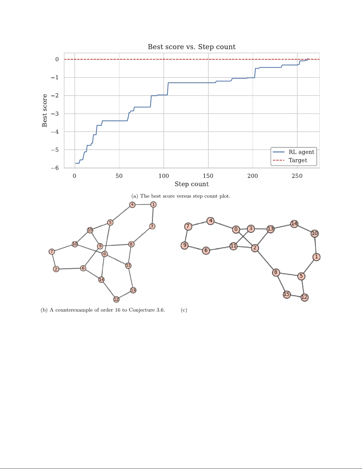
RLGT: A reinforcemen t learning framew ork for extremal graph theory ∗ Iv an Damnjano vić † 1,2 , Uroš Miliv o jević 1 , Irena Ðorđević 1 , and Dragan Stev ano vić ‡ 3 1 F aculty of Ele ctronic Engine ering, University of Niš, Aleksandr a Me dve deva 4, Niš, 18104, Serbia 2 F aculty of Mathematics, Natur al Sciences and Information T e chnolo gies, University of Primorska, Glagoljaška 8, Kop er, 6000, Slovenia 3 Col le ge of Inte gr ative Studies, Ab dul lah Al Salem University, Fir dous Str e et, Blo ck 3, Khaldiya, 72303, Kuwait Abstract Reinforcemen t learning (RL) is a subﬁeld of machine learning that focuses on developing models that can autonomously learn optimal decision-making strategies o ver time. In a recent pioneering paper, W agner demonstrated how the Deep Cross-En tropy RL metho d can b e applied to tac kle v arious problems from extremal graph theory by reformulating them as com binatorial optimization problems. Subsequently , man y researc hers b ecame in terested in reﬁning and extending the framework in tro duced b y W agner, thereb y creating v arious RL en vironments specialized for graph theory . Moreo ver, a num b er of problems from extremal graph theory w ere solved through the use of RL. In particular, sev eral inequalities concerning the Laplacian spectral radius of graphs w ere refuted, new low er b ounds were obtained for certain Ramsey n umbers, and con tributions w ere made to the T urán-type extremal problem in which the forbidden structures are cycles of length three and four. Here, w e presen t Reinforcemen t Learning for Graph Theory (RLGT), a nov el RL framework that systematizes the previous w ork and provides supp ort for both undirected and directed graphs, with or without lo ops, and with an arbitrary num b er of edge colors. The framework eﬃcien tly represen ts graphs and aims to facilitate future RL-based research in extremal graph theory through optimized computational p erformance and a clean and mo dular design. Keyw ords: reinforcemen t learning, extremal graph theory , conjecture solving, machine learning. Mathematics Sub ject Classiﬁcation: 68T05, 68T07, 05C35. 1 In tro duction Reinforcemen t learning (RL) is a subﬁeld of machine learning (ML) that deals with dev eloping mo dels that automatically learn optimal decisions ov er time [33]. A t a high level, an RL system comprises an agen t and an en vironment, with the agent iteratively interacting with the en vironment b y performing actions on it, and the en vironment providing feedbac k in return through observ ations and rewards. In an RL setting, the agent aims to discov er a strategy , called the p olicy , whic h should maximize the long-term success of its actions with resp ect to the rewards returned by the environmen t. Since the agent learns purely by interacting with the en vironment without having an y additional information on the problem b eing solv ed, RL is considered to be muc h more fo cused on goal-directed learning through interaction than other ML paradigms [50]. A com binatorial optimization problem is any problem where a given function f : C → R should b e maximized (resp. minimized) ov er a ﬁnite set of conﬁgurations C . As it turns out, the RL formalism can naturally b e adapted to tackle suc h problems; see [34] and the references therein. This can b e ac hieved b y considering an RL en vironment whose states corresp ond to complete (or partial) conﬁgurations, and where the rewards indicate ho w an action impro ves or worsens a giv en conﬁguration with resp ect to f . Here, we consider the applications of RL to solving combinatorial optimization problems p ertaining to graphs, i.e., extremal graph theory problems. Recen tly , W agner [54] demonstrated how RL can be successfully used to construct coun terexamples that refute graph theory conjectures. His idea was to create an RL environmen t that constructs simple undirected ∗ This researc h was supp orted and funded b y the Ministry of Science, T echnological Dev elopment and Innov ation of the Republic of Serbia, grant n umber 451-03-137/2025-03/200102, and the Science F und of the Republic of Serbia, grant #6767, Lazy walk counts and sp ectral radius of threshold graphs — LZWK. † Corresponding author. ‡ On leav e from the Mathematical Institute of the Serbian Academ y of Sciences and Arts. 1 graphs of a given order n ∈ N b y arranging the  n 2  unordered pairs of vertices in some manner and executing  n 2  binary actions that corresp ond to these pairs. Here, if the i -th action is 1 , then the vertices in the i -th pair should b e adjacen t; otherwise, they should not b e adjacen t. Additionally , a reward is received only after the ﬁnal action is executed, and it should equal a conﬁgurable graph inv ariant f of the constructed graph. Although suc h an environmen t is simple, W agner sho wed that the Deep Cross-Entrop y method [7, 43] can be used in conjunction with it to achiev e satisfactory results for the problem of maximizing a graph inv arian t f ov er the set of graphs of a giv en order. As a direct consequence, it is p ossible to dispro ve inequalities in volving graphs b y transforming the expression L ( G ) ⩽ R ( G ) to L ( G ) − R ( G ) ⩽ 0 and ﬁnding a graph whose corresp onding in v ariant is p ositiv e, where L ( G ) (resp. R ( G ) ) denotes the left-hand (resp. right-hand) side of an inequalit y in graph G . With this approach, W agner dispro ved several conjectured claims either b y directly obtaining a coun terexample or by unco vering structural patterns that help ed man ually construct a counterexample. W agner’s approach w as also successfully used in [49] to refute a conjecture by Akbari, Alazemi and Anđelić [2] on the graph energy and the matc hing n umber of graphs. Afterwards, Ghebleh et al. [24] oﬀered a reimple- men tation of W agner’s approac h to increase its readabilit y , stability and computational performance. In this framew ork, the Deep Cross-Entrop y metho d was again used in conjunction with the RL en vironment introduced b y W agner, but the op erations inv olving states w ere notably implemented more eﬃciently through NumPy -based v ectorization [30]. A dditionally , the ﬁnal reward function was turned in to a separate argumen t so that it could optionally b e executed more eﬃciently using external co de, e.g., Java co de using JPype [37]. With this ap- proac h and by applying the features from the graph6java library [25], the authors succeeded in dispro ving sev eral previously conjectured upp er bounds on the Laplacian sp ectral radius of graphs [10]. W e brieﬂy note that T aieb et al. [52] successfully refuted t wo more of these upp er b ounds by applying the Monte Carlo search tec hnique. Using the same framework dev elop ed in [24], Ghebleh et al. [23] obtained four new lo wer b ounds on small Ramsey num b ers in volving complete bipartite graphs, wheel graphs and bo ok graphs [41]. Afterwards, this framew ork w as used once again by the same authors [22] to help obtain an explicit construction of harmonic graphs [42] with arbitrarily many distinct vertex degrees. Concurren tly , Mehrabian et al. [36] used RL to tackle the T urán-type extremal problem [46] originally p osed b y Erdős [20] in 1975, in which the forbidden structures are cycles of length three and four. In their approach, a diﬀeren t RL environmen t w as used, where the states are all the graphs of a given order and the actions are edge- ﬂipping op erations. By incorp orating curriculum learning [48] into the AlphaZero [45] and tabu search [26, 27] algorithms, they obtained new lo wer b ounds for n ∈ { 64 , 65 , 66 , . . . , 134 } , where n is the graph order. W e men tion in passing that this was achiev ed through a nov el neural netw ork architecture called the Pairformer. In a subsequent pap er, Angileri et al. [4] systematized the previous work by implementing four distinct RL en vironments sp ecialized for graph theory: Linear, Lo cal, Global and Flip. Here, the Linear environmen t is based on W agner’s original approach [54], while Flip is precisely the edge-ﬂipping en vironmen t from the pap er of Mehrabian et al. [36]. The four RL environmen ts were implemented in the ob ject-orien ted paradigm as classes that inherit from the Env class from the Gymnasium library [53], and their states provide supp ort for ﬁnite undirected graphs without m ultiple edges, with or without loops. Additionally , the authors introduced a no vel dataset of graphs lab eled with their Laplacian sp ectra for the purpose of facilitating research inv olving the Laplacian sp ectral prop erties of graphs. Later on, Angileri et al. [5] oﬀered a mo diﬁcation of their RL framew ork and applied it to contribute to the study of Brouw er’s conjecture [11]. W e present Reinforcemen t Learning for Graph Theory (RLGT), a no vel RL framew ork sp ecialized for ex- tremal graph theory that aims to systematize the previous work and bridge the gap b et ween the computationally eﬃcien t approach of Ghebleh et al. [22–24] and the more expressive and ﬂexible approach of Angileri et al. [4, 5]. The framework is implemented in the ob ject-oriented paradigm as a pro ject in the programming language Python , and it is based on the following principles. (1) T o mak e the framew ork fully mo dularized while k eeping the pro ject structure clean, we split the pro ject in to three pack ages: graphs , environments and agents . (2) The graphs pack age contains the core class that enables the user to conv eniently represen t graphs in eight p ossible formats and automatically p erform conv ersions b et ween these formats. This is an impro vemen t o ver the previous approac hes, where no such class existed and the graph format conv ersions w ere left to the end user. (3) Besides represen ting graphs, the graphs pac k age is also capable of representing a batch of graphs as a single ob ject. This is inspired b y the approach of Ghebleh et al. [22–24] and it enables the operations in volving graphs and states to b e p erformed more eﬃciently through NumPy -based vectorization. (4) The graphs and batches of graphs represented in the graphs pack age can b e either undirected or directed, and may or ma y not ha ve lo ops. Essen tially , the only requiremen t is that the represented undirected 2 (resp. directed) graph is ﬁnite and has no m ultiple edges (resp. arcs). A dditionally , the edges (resp. arcs) can b e colored in an arbitrary num b er of colors, whic h pro vides direct support for problems inv olving edge coloring [12]. This extends the previous work, where there was no supp ort for directed graphs or for graphs with more than tw o edge colors. (5) The environments pack age contains the class implementations of RL environmen ts sp ecialized for graph theory . The implemented environmen ts are largely inspired by the approach of Angileri et al. [4, 5]. W e pro vide nine diﬀerent en vironments realized as sev en classes. (6) The agents pac k age con tains the classes corresponding to three diﬀerent RL methods to b e used in conjunction with the av ailable RL environmen ts. This improv es the previous frameworks, where either the pro ject structure was not mo dularized, or the agents were not encapsulated as fully separate entities. The three a v ailable RL metho ds are the Deep Cross-En tropy metho d [7, 43], the REINFOR CE metho d [55], and the Pro ximal Policy Optimization (PPO) metho d [44], and they are all implemented using PyTorch [39]. (7) T o increase stabilit y and repro ducibilit y , we use the Poetry to ol [21] for Python pack aging and dep endency managemen t. In addition, the co de clarit y is impro ved through the Black [32] and isort [13] to ols. Finally , the pytest testing framework [31] is applied to unit-test the framework features, additionally increasing the pro ject stability . In Section 2, we present the graph-theoretic and RL foundations on which the prop osed framework is based. Afterw ards, w e give an o verview of the developed framework in Section 3 and provide justiﬁcations for man y of its implementation details. In Section 4, we provide three applications to concrete graph theory problems that demonstrate the framew ork’s ease of use and eﬃciency . Finally , in Section 5, w e end the pap er with a brief conclusion and discuss possible directions for future work. The Python implemen tation of the presented RL framework can b e found in [16], while the do cumen tation is a v ailable in [15] and the Python Pac k age Index (PyPI) page is av ailable in [17]. 2 Preliminaries In this section, w e in tro duce the basic deﬁnitions from graph theory and RL that are required to comprehend the prop osed framework design and implementation. 2.1 Graph theory All undirected graphs are assumed to b e ﬁnite and without multiple edges, and we consider all directed graphs to b e ﬁnite and without multiple arcs. In particular, lo ops are allo wed in b oth undirected and directed graphs. W e use the term gr aph to refer to either an undirected graph or a directed graph, and we denote the vertex set of a graph G by V ( G ) and the edge set by E ( G ) . The or der of a graph G is the num b er of vertices it con tains, i.e., | V ( G ) | . F or conv enience, we assume that V ( G ) = { 0 , 1 , 2 , . . . , n − 1 } for an y graph G of order n . A dditionally , we assume that all vector, matrix or tensor indexing is zero-based. The adjac ency matrix of a graph G of order n , denoted by A ( G ) , is the binary matrix in R n × n deﬁned by A ( G ) u,v = ( 1 , if u is adjacent to v , 0 , otherwise (0 ⩽ u, v ⩽ n − 1) . Recall that if the graph G is undirected, then A ( G ) is a symmetric matrix. F or other undeﬁned terminology from elementary graph theory , the reader can refer to the standard literature [6, 8, 9, 11, 14, 18, 28]. F or any k ∈ N , a k -e dge-c olor e d lo op e d c omplete undir e cte d gr aph is an undirected graph that con tains all p ossible edges, including lo ops, with each edge being labeled b y a color from the set { 0 , 1 , 2 , . . . , k } . Here, the n umbers 0 , 1 , 2 , . . . , k − 1 represen t the k prop er edge colors, while the n umber k can b e optionally used to lab el an edge that is uncolored, i.e., not colored y et. Similarly , for any k ∈ N , a k -e dge-c olor e d lo op e d c omplete dir e cte d gr aph is a directed graph that contains all p ossible arcs, including lo ops, with eac h arc b eing lab eled by a color from the set { 0 , 1 , 2 , . . . , k } . W e sa y that a k -edge-colored lo op ed complete undirected (resp. directed) graph is ful ly c olor e d if no edge (resp. arc) is labeled by the num b er k . An y undirected graph G can b e view ed as a 2 -edge-colored lo oped complete undirected graph of the same order by coloring the edges of G with the color 1 and the remaining edges with the color 0 . Therefore, undirected graphs naturally corresp ond to 2 -edge-colored lo oped complete undirected graphs. Analogously , directed graphs corresp ond to 2 -edge-colored lo oped complete directed graphs. With this in mind, we can use the k -edge-colored lo oped complete graphs to represent b oth graphs whose edges or arcs are inheren tly colored and those used in extremal graph theory problems without edge coloring. 3 2.2 Reinforcemen t learning In practice, an RL task is typically mo deled as a Markov De cision Pr o c ess (MDP), deﬁned as an ordered triple ( S , A , p ) , where S is the state space, A is the action space, and p : S × A → ∆( S × R ) is the transition function, with ∆( · ) denoting the set of probability distributions ov er its argumen t. Here, p ( s ′ , r | s, a ) is the probability of reac hing the next state s ′ and receiving the rew ard r after the action a is executed in the curren t state s . A p olicy is a strategy used by the agent to select actions while in teracting with the environmen t, formalized as a function π : S → ∆( A ) . An episo dic task is an RL task where a terminal state is even tually reached regardless of ho w the agent acts on the en vironment, whereas a c ontinuing task is one without terminal states, in whic h the agent–en vironment interaction can pro ceed indeﬁnitely . F or further details on RL theory and terminology , the reader can refer to the standard textb o oks [33, 40, 50, 51]. W e consider the problem of maximizing the function f ov er the set of fully colored k -edge-colored loop ed complete (undirected or directed) graphs of order n , for a giv en n ⩾ 2 , k ⩾ 2 and graph in v ariant f . W e are th us only interested in RL tasks designed to build such graphs. T o b egin, we consider only deterministic tasks, whic h means that whenever an action a is executed in a state s , the same next state s ′ is alw ays reac hed and the same rew ard r is alwa ys received. Therefore, we can formalize the transition model through a function of the form S × A → S × R instead of the more general S × A → ∆( S × R ) . Besides, we assume that an RL task is either con tin uing, like the edge-ﬂipping environmen t in tro duced by Mehrabian et al. [36], or it is episo dic and a terminal state is reached after a predetermined num b er of actions, regardless of how the actions are selected, lik e the en vironment from W agner’s original approach [54]. In the case of contin uing tasks, the RL environmen t receiv es a parameter that determines the total n um b er of actions to b e executed within eac h episo de. T o make the graph inv ariant f a fully conﬁgurable parameter of the RL environmen t, we separate the logic b ehind the state transition and the rew ard computation. F or any choice of f , we assume that the same state s ′ is reached from a state s when an action a is executed. Hence, the state transition can b e mo deled through a function of the form t : S × A → S , where s ′ = t ( s, a ) . Additionally , we assume that each state s has an underlying (not necessarily fully colored) k -edge-colored lo oped complete graph φ ( s ) . As for the rew ard computation, our approach is to use graph in v ariant v alues rather than con ven tional RL rewards. In other w ords, when the environmen t reaches a state s , the agen t receives the v alue f ( φ ( s )) . W e believe that such an agent–en vironment interaction is natural in the context of tack ling extremal graph theory problems. In addition, we recognize tw o types of agent–en vironmen t communication settings: sparse and dense. If an RL en vironment uses the sp arse setting , then the attained graph inv arian t is received only after the ﬁnal action, and f ( φ ( s )) need not b e deﬁned for non-ﬁnal states s . Con versely , if the environmen t uses the dense setting , then the attained graph in v ariant is receiv ed after eac h executed action. In the previous work, W agner [54] and Ghebleh et al. [22–24] used the sparse setting, while Mehrabian et al. [36] essentially used the dense setting through telescopic rewards. Our approach is partially inspired by Angileri et al. [4, 5], hence we supp ort b oth communication settings in a mo dularized and clean manner. 3 F ramew ork o v erview The presented RL framew ork was implemen ted in the programming language Python . Although there are more computationally eﬃcient languages, suc h as C , C++ , C# , Java , Rust and Go [38], our choice of language is justiﬁed b y the full supp ort of the tw o well-kno wn deep learning libraries PyTorch [39] and TensorFlow [1] in Python . A dditionally , the vectorized op erations in NumPy pro vide satisfactory computational eﬃciency , especially when executed on a mo dern high-end computer. Finally , due to the expressive p ow er of Python , the framew ork can b e used without extensiv e prior programming exp erience, making it accessible to a wide sp ectrum of end use r s. The framework implementation can b e found in [16], while the do cumen tation is av ailable in [15] and the PyPI page is av ailable in [17]. F or the sak e of modularity , the framework is split into three pack ages: graphs , environments and agents . The graphs pack age encapsulates graphs and batches of graphs, representing them in eight p ossible formats and automatically p erforming all required conv ersions b et w een these formats. The environments pack age contains nine RL en vironments implemented as sev en classes that provide supp ort for v arious graph-building games. A dditionally , this pack age contains several auxiliary functions that help create deterministic or nondeterministic graph generators. The agents pac k age contains the three RL agents corresp onding to the Deep Cross-Entrop y , REINF ORCE, and PPO metho ds, alongside sev eral classes that implement random action mec hanisms. The dep endencies b et ween the three pac k ages are clean, with the graphs pack age ha ving no dep endencies on the other tw o pack ages, and the environments pack age depending only on the graphs pack age. Therefore, the pac k ages follow a lay ered design. The Poetry to ol is used for Python pack aging and dep endency management. The ﬁrst t wo pack ages, graphs and environments , hav e no external dep endencies apart from NumPy , while the third pac k age, agents , addi- tionally dep ends only on PyTorch . F or extendability , only NumPy is considered an obligatory dep endency , while 4 PyTorch is not installed by default. This allo ws the end user to potentially emplo y another deep learning library instead of PyTorch . F or instance, if the user prefers TensorFlow to PyTorch , they can perform the default installation and use only the graphs and environments pack ages together with their own RL metho ds implemen ted in TensorFlow . Alternativ ely , PyTorch can b e installed as an optional dependency , enabling the use of the three av ailable RL methods, all of which are implemented in PyTorch . This approac h highlights the mo dularit y of the framew ork and is natural, since ha ving t wo deep learning libraries installed at the same time is typically undesirable, esp ecially if only one of them is used. T o increase the pro ject stability , pytest is applied to unit-test the framework features. W e additionally use Black and isort to improv e the co de clarity . 3.1 Graphs and graph formats The core comp onen t of the graphs pack age is the Graph class, whic h encapsulates the concept of a k -edge- colored loop ed complete graph. The class essentially b eha v es as a wrapp er around a collection of eight NumPy arra ys, eac h of whic h represents the graph in one of the eigh t supp orted graph formats. Apart from sev eral prop erties, the main functionality that distinguishes the class from a pure o ctuple is the automatic conv ersion b et ween these eight formats. W e view a k -edge-colored lo oped complete graph as a quintuple (edge_colors, is_directed, allow_loops, graph_format, format_representation) , where: (1) edge_colors is the num b er of prop er edge colors, i.e., k , with the requirement that k ⩾ 2 ; (2) is_directed is a b oolean indicating whether the considered graph is a k -edge-colored lo oped complete directed graph or a k -edge-colored loop ed complete undirected graph; (3) allow_loops is a b oolean indicating whether the considered graph is allow ed to hav e lo ops; (4) graph_format is one of the eight supp orted graph formats; and (5) format_representation is the NumPy array represen ting the structure of the considered graph in the c hosen graph format. Although the presence of lo ops can b e inferred from the graph structure, we use this representation b ecause the elements edge_colors , is_directed and allow_loops directly aﬀect how the format_representation NumPy arra y is used to obtain the considered graph. W e provide support for the following eight graph formats. (1) The bitmask format for the out-neighb orho o ds represents the graph structure through a matrix B ∈ Z k × n , where k is the n umber of prop er edge colors and n is the graph order. All entries of B are integers b et ween 0 and 2 n − 1 , so that for any c ∈ { 0 , 1 , 2 , . . . , k − 1 } and u, v ∈ { 0 , 1 , 2 , . . . , n − 1 } , the v -th bit in the binary represen tation of B c,u is one if and only if the edge (resp. arc) from vertex u to v ertex v has color c . If lo ops are not allo wed, then the u -th bit of B c,u is taken to b e zero for any c ∈ { 0 , 1 , 2 , . . . , k − 1 } and u ∈ { 0 , 1 , 2 , . . . , n − 1 } . (2) The bitmask format for the in-neighb orho o ds represents the graph structure in the same w ay as the bitmask format for the out-neighborho ods, with the diﬀerence that the v -th bit of B c,u indicates whether the edge (resp. arc) from vertex v to vertex u has color c , instead of the edge (resp. arc) from vertex u to vertex v . These tw o formats coincid e if the considered graph is undirected. (3) The adjac ency matrix format with c olor numb ers employs a v ariant of the adjacency matrix to represen t the graph structure. More precisely , this format uses a matrix A ∈ Z n × n , where n is the graph order, suc h that for any u, v ∈ { 0 , 1 , 2 , . . . , n − 1 } , the entry A u,v is equal to the color of the edge (resp. arc) from v ertex u to v ertex v . Recall that an uncolored edge (resp. arc) is represented b y the color k , where k is the num b er of prop er edge colors. If lo ops are not allow ed, then the diagonal entries of A are all equal to zero. Moreo ver, if the considered graph is undirected, then the matrix A is symmetric. (4) The adjac ency matrix format with binary slic es is similar to the adjacency matrix format with color n umbers, with the diﬀerence that the colors correspond to separate binary matrices instead of b eing represen ted by integer v alues in a single matrix. More precisely , this format emplo ys a binary tensor A ∈ Z k × n × n , where k is the num b er of proper edge colors and n is the graph order, such that for an y c ∈ { 0 , 1 , 2 , . . . , k − 1 } and u, v ∈ { 0 , 1 , 2 , . . . , n − 1 } , the entry A c,u,v equals one if and only if the edge (resp. arc) from vertex u to v ertex v has color c . If lo ops are not allo wed, then A c,u,u = 0 for an y c ∈ { 0 , 1 , 2 , . . . , k − 1 } and u ∈ { 0 , 1 , 2 , . . . , n − 1 } . (5) The ﬂattene d r ow-major format with c olor numb ers represents the graph structure through a vector in Z ℓ con taining the entries of the matrix A from the adjacency matrix format with color num b ers, arranged in ro w-ma jor order. In other words, the entries are arranged so that the ﬁrst ro w is trav ersed from left to 5 righ t, then the second ro w is trav ersed from left to right, and so on until the last row. Additionally , all redundancy in data storage is av oided. More precisely , if the considered graph is directed and lo ops are not allow ed, then the diagonal entries are omitted. If the graph is undirected, then only the entries from the upp er triangular part of A are arranged in ro w-ma jor order, with or without the diagonal, dep ending on whether lo ops are allow ed. Therefore, ℓ =          n 2 , if the considered graph is directed and lo ops are allow ed , n 2 − n, if the considered graph is directed and lo ops are not allow ed ,  n +1 2  , if the considered graph is undirected and lo ops are allow ed ,  n 2  , if the considered graph is undirected and lo ops are not allow ed , (1) where n is the graph order. (6) The ﬂattene d r ow-major format with binary slic es is similar to the ﬂattened ro w-ma jor format with color n umbers, with the diﬀerence that the colors corresp ond to separate binary vectors instead of being rep- resen ted b y in teger v alues in a single v ector. This format emplo ys a binary matrix F ∈ Z k × ℓ , where k is the num b er of prop er edge colors and ℓ is given b y (1), such that for an y c ∈ { 0 , 1 , 2 , . . . , k − 1 } and i ∈ { 0 , 1 , 2 , . . . , ℓ − 1 } , the en try F c,i equals one if and only if the i -th edge (resp. arc) has color c . Here, the edges (resp. arcs) are assumed to b e arranged in row-ma jor order. (7) The ﬂattene d clo ckwise format with c olor numb ers represents the graph structure in the same w ay as the ﬂattened row-ma jor format with color n umbers, with the diﬀerence that the edges (resp. arcs) are arranged in clo c kwise order instead of row-ma jor order. By clo c kwise order, we mean the order (0 , 0) , (0 , 1) , (1 , 1) , (1 , 0) , (0 , 2) , (1 , 2) , (2 , 2) , (2 , 1) , (2 , 0) , . . . , where the en tries are trav ersed in a clockwise lay er-like manner. Note that if the considered graph is undirected, then the obtained order can equiv alently b e regarded as the column-ma jor order ov er the upp er triangular part of the adjacency matrix. (8) The ﬂattene d clo ckwise format with binary slic es uses the same approach to represent the graph structure as the ﬂattened ro w-ma jor format with binary slices, with the diﬀerence that the edges (resp. arcs) are arranged in clo c kwise order instead of row-ma jor order. T o further reduce redundancy in data storage, we can omit the entries corresp onding to color zero in the bitmask formats and the formats with binary slices, pro vided the considered graph is fully colored. F or example, a bitmask format representation of a fully colored graph can b e given as a matrix in Z ( k − 1) × n instead of Z k × n , where the ro ws corresp ond to colors 1 , 2 , . . . , k − 1 , resp ectiv ely . W e refer to such a format as a r e duc e d format . These format v ariants are w ell deﬁned because if the considered graph is fully colored, then an edge has color zero if it has no color from { 1 , 2 , . . . , k − 1 } , and we can infer whether the giv en format is reduced from the shap e of the format_representation NumPy arra y . Moreo ver, it is natural to ignore color zero for practical reasons in the frequent case where k = 2 . T wo examples of k -edge-colored lo oped complete directed graphs in all eigh t supp orted formats are sho wn in T able 1, and tw o examples of k -edge-colored lo op ed complete undirected graphs in all eight supp orted formats are sho wn in T able 2. Instances of the Graph class are initialized through a pro vided representation quin tuple (edge_colors, is_directed, allow_loops, graph_format, format_representation) . A dditionally , the end user can ini- tialize an instance in more than one graph format, in whic h case all provided format representations need to b e consisten t with one another, i.e., they must represen t the same graph. Afterw ards, the graph can b e accessed in an y of the eight supp orted formats by simply using the corresp onding prop ert y , with all format conv ersions b e- ing p erformed automatically . When conv erting to a bitmask format or a format with binary slices, the reduced format v ariant is alwa ys used when p ossible. Example 3.1. The graph G 1 from T able 1 can be initialized using the Graph constructor as follows. 1 flattened_row_major_colors = np.array( 2 [2, 2, 2, 0, 3, 3, 3, 0, 3, 2, 1, 2, 1, 2, 3, 1], 3 dtype=np.uint8, 4 ) 5 g1 = Graph( 6 edge_colors=3, 7 is_directed=True, 8 allow_loops=True, 9 flattened_row_major_colors=flattened_row_major_colors, 10 ) 6 Graph G 1 Graph G 2 edge_colors 3 3 is_directed True True allow_loops True False Bitmask format for the out-neighborho ods h 8 8 0 0 0 0 4 9 7 0 10 2 i  8 12 0 0 6 0 9 2  Bitmask format for the in-neighborho ods h 0 0 0 3 8 0 4 8 1 13 1 4 i  0 0 2 3 4 9 1 4  A djacency matrix format with color num b ers  2 2 2 0 3 3 3 0 3 2 1 2 1 2 3 1   0 2 2 1 0 0 1 1 2 0 0 2 0 2 0 0  A djacency matrix format with binary slices  0 0 0 1 0 0 0 1 0 0 0 0 0 0 0 0  ,  0 0 0 0 0 0 0 0 0 0 1 0 1 0 0 1  ,  1 1 1 0 0 0 0 0 0 1 0 1 0 1 0 0   0 0 0 1 0 0 1 1 0 0 0 0 0 0 0 0  ,  0 1 1 0 0 0 0 0 1 0 0 1 0 1 0 0  Flattened row-ma jor format with color num b ers  2 2 2 0 3 3 3 0 3 2 1 2 1 2 3 1  ⊺  2 2 1 0 1 1 2 0 2 0 2 0  ⊺ Flattened row-ma jor format with binary slices h 0 0 0 1 0 0 0 1 0 0 0 0 0 0 0 0 0 0 0 0 0 0 0 0 0 0 1 0 1 0 0 1 1 1 1 0 0 0 0 0 0 1 0 1 0 1 0 0 i  0 0 1 0 1 1 0 0 0 0 0 0 1 1 0 0 0 0 1 0 1 0 1 0  Flattened clo c kwise format with color num b ers  2 2 3 3 2 3 1 2 3 0 0 2 1 3 2 1  ⊺  2 0 2 1 0 2 1 1 2 0 2 0  ⊺ Flattened clo c kwise format with binary slices h 0 0 0 0 0 0 0 0 0 1 1 0 0 0 0 0 0 0 0 0 0 0 1 0 0 0 0 0 1 0 0 1 1 1 0 0 1 0 0 1 0 0 0 1 0 0 1 0 i  0 0 0 1 0 0 1 1 0 0 0 0 1 0 1 0 0 1 0 0 1 0 1 0  T able 1: A directed graph G 1 with allow ed lo ops and a directed graph G 2 without allow ed lo ops, both represented in all eight supp orted graph formats. A reduced format is alwa ys used when p ossible. Here, the graph is initialized in the ﬂattened row-ma jor format with color num b ers, and it can then b e accessed in any of the eight supp orted graph formats. 1 print (g1.bitmask_out) 2 print (g1.bitmask_in) 3 print (g1.adjacency_matrix_colors) 4 print (g1.adjacency_matrix_binary) 5 print (g1.flattened_row_major_colors) 6 print (g1.flattened_row_major_binary) 7 print (g1.flattened_clockwise_colors) 8 print (g1.flattened_clockwise_binary) In addition, the Graph class con tains three class metho ds that enable the user to instan tiate a Graph ob ject in exactly one sp eciﬁc type of graph format. F or example, the graph G 2 from T able 1 can b e initialized in the bitmask format for the out-neighborho ods as follows. 1 bitmask = np.array( 2 [ 3 [8, 12, 0, 0], 4 [6, 0, 9, 2], 5 ], 6 dtype=np.uint64, 7 ) 8 g2 = Graph.from_bitmask( 9 bitmask=bitmask, 10 bitmask_type=BitmaskType.OUT_NEIGHBORS, 11 edge_colors=3, 12 is_directed=True, 13 allow_loops=False, 14 ) The follo wing co de snippet initializes the graph G 3 from T able 2 in the adjacency matrix format with binary slices. 7 Graph G 3 Graph G 4 edge_colors 4 2 is_directed False False allow_loops True False Bitmask format for the out-neighborho ods  2 1 0 1 4 2 4 0 1 0 2 0   12 24 25 23 14  Bitmask format for the in-neighborho ods  2 1 0 1 4 2 4 0 1 0 2 0   12 24 25 23 14  A djacency matrix format with color num b ers h 1 0 2 0 3 1 2 1 4 i " 0 0 1 1 0 0 0 0 1 1 1 0 0 1 1 1 1 1 0 1 0 1 1 1 0 # A djacency matrix format with binary slices hh 0 1 0 1 0 0 0 0 0 i , h 1 0 0 0 0 1 0 1 0 i , h 0 0 1 0 0 0 1 0 0 i , h 0 0 0 0 1 0 0 0 0 ii "" 0 0 1 1 0 0 0 0 1 1 1 0 0 1 1 1 1 1 0 1 0 1 1 1 0 ## Flattened row-ma jor format with color num b ers  1 0 2 3 1 4  ⊺  0 1 1 0 0 1 1 1 1 1  ⊺ Flattened row-ma jor format with binary slices  0 1 0 0 0 0 1 0 0 0 1 0 0 0 1 0 0 0 0 0 0 1 0 0   0 1 1 0 0 1 1 1 1 1  Flattened clo c kwise format with color num b ers  1 0 3 2 1 4  ⊺  0 1 0 1 1 1 0 1 1 1  ⊺ Flattened clo c kwise format with binary slices  0 1 0 0 0 0 1 0 0 0 1 0 0 0 0 1 0 0 0 0 1 0 0 0   0 1 0 1 1 1 0 1 1 1  T able 2: An undirected graph G 3 with allow ed lo ops and an undirected graph G 4 without allow ed lo ops, b oth represen ted in all eigh t supp orted graph formats. A reduced format is alwa ys used when p ossible. 1 adjacency_matrix = np.array( 2 [ 3 [ 4 [0, 1, 0], 5 [1, 0, 0], 6 [0, 0, 0], 7 ], 8 [ 9 [1, 0, 0], 10 [0, 0, 1], 11 [0, 1, 0], 12 ], 13 [ 14 [0, 0, 1], 15 [0, 0, 0], 16 [1, 0, 0], 17 ], 18 [ 19 [0, 0, 0], 20 [0, 1, 0], 21 [0, 0, 0], 22 ], 23 ], 24 dtype=np.uint8, 25 ) 26 g3 = Graph.from_adjacency_matrix( 27 adjacency_matrix=adjacency_matrix, 28 color_representation=ColorRepresentation.BINARY_SLICES, 29 edge_colors=4, 30 is_directed=False, 31 allow_loops=True, 32 ) 8 The graph G 4 from T able 2 can be initialized in the ﬂattened clo c kwise format with color num b ers as follows. 1 flattened = np.array([0, 1, 0, 1, 1, 1, 0, 1, 1, 1], dtype=np.uint8) 2 g4 = Graph.from_flattened( 3 flattened=flattened, 4 flattened_ordering=FlattenedOrdering.CLOCKWISE, 5 color_representation=ColorRepresentation.COLOR_NUMBERS, 6 ) Note that by default, a graph is considered undirected, without lo ops, and with tw o prop er edge colors. There- fore, all the corresponding parameters can be omitted when the default v alues are suﬃcien t. The full source co de for Example 3.1 is av ailable in the ﬁle examples/graph_examples.py in [16]. ♢ Besides k -edge-colored lo oped complete graphs, the Graph class also encapsulates batc hes of k -edge-colored lo oped complete graphs. In this case, the graphs in the batc h are required to b e of the same order and with the same num b er of prop er edge colors, and they need to b e of the same t yp e: they are either all directed or all undirected, and either all of them ha ve allo wed loops or none of them ha ve allo wed loops. This enables such batc hes of graphs to be represen table using the same eight graph formats by simply using a NumPy array of one dimension higher. In such format represen tations, the leading dimension corresp onds to the graphs in the batc h, while the remaining dimensions are used in the same w a y as when representing single graphs. It is easy to infer whether a Graph ob ject represen ts a graph or a batch of graphs through the batch_size prop ert y — for batc hes of graphs, it returns the n um b er of graphs in the batch, while for single graphs, it returns None . In addition to the Graph class, the graphs pac k age also con tains several classes that inherit from this class and encapsulate k -edge-colored lo oped complete graphs with some particular structure. W e provide the following classes that inherit from the Graph class: (1) MonochromaticGraph ; (2) EmptyGraph ; (3) CompleteGraph ; (4) AlmostCompleteGraph ; (5) CompleteBipartiteGraph ; (6) CompleteKPartiteGraph ; (7) StarGraph ; (8) PathGraph ; (9) CycleGraph ; (10) WheelGraph ; (11) BookGraph ; and (12) FriendshipGraph . The name of each of these classes determines the kind of graphs it encapsulates. W e mention in passing that all of these graphs ha ve tw o prop er edge colors, besides the graphs encapsulated by the MonochromaticGraph class, which can hav e any n umber of prop er edge colors. F or more details, the reader can refer to the framework do cumen tation [15]. 3.2 RL en vironmen ts The environments pack age contains the abstract class GraphEnvironment , whic h encapsulates RL environmen ts in extremal graph theory applications, alongside several concrete classes that inherit from this class. The t wo primary metho ds of the GraphEnvironment class are reset_batch , which initializes a batch of episo des with a giv en batc h size, and step_batch , whic h tak es a batch of actions and applies them element-wise to the curren t states from the ongoing episodes. These tw o metho ds follo w a Gymnasium -lik e API and naming con ven tion, with the exception that they op erate in batc h mo de. In other words, multiple episo des can b e run and acted on in parallel to increase eﬃciency through NumPy -based vectorization. This strategy is inspired by the approach of Ghebleh et al. [22–24], and it relies on our assumption that all episodes end after a predetermined n umber of actions, regardless of whether the environmen t has contin uing or episo dic RL tasks. The states in an RL environmen t are represented as NumPy vectors of some length and type speciﬁc to the concrete class that inherits from GraphEnvironment . Naturally , batc hes of states are then represented as NumPy matrices of the required shap e and type, with ro ws corresp onding to the states in the batch. It is assumed that there are ﬁnitely many actions, and they are represented by nonnegative integers from { 0 , 1 , 2 , . . . , q − 1 } , where q ⩾ 2 is the total num b er of actions. Similarly , batc hes of actions are represented as NumPy vectors of type numpy.int32 whose entries corresp ond to the actions. W e mention in passing that not every action needs to b e a v ailable for execution at every step, b ut at least one action should b e av ailable in any non-terminal state. Although the reset_batch and step_batch metho ds serve entirely diﬀeren t purp oses, they b oth return the same triple: (1) the batch of states, obtained up on initialization or after applying the provided actions element-wise to the previous states; 9 (2) the batch of graph inv ariant v alues, computed only when required b y the agen t–environmen t communica- tion setting; and (3) the curren t status of the batch of episo des. W e recognize three p ossible statuses that an episo de may ha ve. (1) An episo de is in pr o gr ess if it is in a state that accepts further actions. (2) An episode has terminate d if it has ended due to reaching a terminal state. This status is only p ossible in RL environmen ts wh ere the tasks are episo dic and terminal states exist. (3) An episode has b een trunc ate d if it has ended b ecause the required num b er of steps has b een tak en. In this case, although the current state is not terminal, no further actions should b e p erformed. This status app ears only in RL environmen ts with contin uing tasks. Since all the episodes in an y batch are guaran teed to end at the same time, they alw a ys ha ve the same status, so w e can deﬁne the status of a batch of episo des as the status of any of its episo des. This is precisely the status that the reset_batch and step_batch methods return. Note that w e purp osefully distinguis h b et ween termination and truncation to keep the API consistent with Gymnasium . In the context of graph in v ariant computation, we recognize tw o types of agent–en vironment communication settings: sparse and dense. This setting is a conﬁgurable parameter of each instance of the GraphEnvironment class and can b e reconﬁgured at any step. (1) If the sparse setting is selected, then no batc h of graph in v ariant v alues is computed after each batch of actions, except after the ﬁnal batch. In that case, the returned v alues are equal to f ( φ ( s )) , where φ ( s ) is the batch of underlying graphs corresp onding to the ﬁnal states, and f is a function that accepts a batch of graphs and returns the corresp onding graph in v ariant v alues. (2) If the dense setting is selected, then a batch of graph inv ariant v alues is computed after each batc h of actions, and it is equal to f ( φ ( s )) , where φ ( s ) is the batch of underlying graphs corresp onding to the newly obtained states. (3) A dditionally , if the dense setting is selected, then the graph in v ariant computation ma y optionally b e carried out using a function ∆ f , which accepts tw o batches of graphs of equal size and returns the elemen t- wise diﬀerences of the corresp onding graph inv ariant v alues. In this case, the reset_batch metho d computes the graph in v ariant v alues using f , and afterw ards, the ste p_batch metho d incrementally up dates them using ∆ f . The idea of optionally using ∆ f in the dense setting is natural, since suc h a diﬀerence function may b e more eﬃcien t than inv oking the original graph inv ariant function f . Although the metho ds reset_batch and step_batch are not abstract, their b eha vior is largely determined b y the abstract methods _initialize_batch , _transition_batch and state_batch_to_graph_batch , all of whic h m ust be implemen ted b y any concrete subclass inheriting from GraphEnvironment . The reset_batch metho d initializes the starting states by in voking _initialize_batch and then computes the graph in v ariant v alues if required. Similarly , the step_batch metho d p erforms the state transition through _transition_batch and subsequently computes the graph in v arian t v alues if required. In both metho ds, the graph inv ariant com- putation inv olves in voking the abstract metho d state_batch_to_graph_batch , which encapsulates φ as a pure function. Therefore, concrete sub classes of GraphEnvironment only need to implement the state initialization and state transition logic, without handling the graph inv arian t computation itself, since this is managed en tirely within the GraphEnvironment class. The concrete classes m ust accept the selected communication setting, the graph inv ariant function f , and optionally the graph in v ariant diﬀerence function ∆ f , as constructor arguments, whic h are then passed to the abstract paren t class. Apart from the three men tioned abstract metho ds, any concrete class that inherits from GraphEnvironment m ust also implement the follo wing six abstract properties: (1) state_length , whic h returns the length of the NumPy v ectors representing the states; (2) state_dtype , whic h returns the t yp e of the NumPy vectors representing the states; (3) action_number , whic h returns the total num b er of actions; (4) action_mask , which determines what actions are currently a v ailable for execution in eac h of the episo des that are b eing run in parallel; 10 (5) episode_length , which returns the predetermined length of all the episodes that are currently running or are to b e run; and (6) is_continuing , whic h determines whether the environmen t has contin uing or episo dic RL tasks. These six prop erties provide the interface that allo ws the agent to in teract with the environmen t. W e provide sev en classes that i nherit from GraphEnvironment and encapsulate nine diﬀeren t RL en viron- men ts. These environmen ts can b e split in to three groups: (1) the linear en vironments, whic h are implemen ted using three separate classes LinearBuildEnvironment , LinearSetEnvironment and LinearFlipEnvironment ; (2) the global environmen ts, which are implemen ted using tw o separate classes GlobalSetEnvironment and GlobalFlipEnvironment ; and (3) the local en vironments, whic h are implemented using t wo separate classes LocalSetEnvironment and LocalFlipEnvironment . The class naming is largely inspired b y the work of Angileri et al. [4, 5]. Moreov er, our sev en classes are implemen ted using similar ideas, with the distinction that supp ort is now also pro vided for directed graphs and graphs with more than tw o edge colors, and the agent–en vironment in teraction logic is fully encapsulated on the agent side, with the agent treated as a separate entit y . 3.2.1 Linear environmen ts The LinearBuildEnvironment class implemen ts the Linear Build en vironment, which is directly based on W agner’s original approac h. This environmen t m odels a graph-building game in whic h the edges (resp. arcs) are initially uncolored and are then prop erly colored one by one, either in row-ma jor or clo c kwise order. The user can select the graph order n ⩾ 2 and the num b er of prop er edge colors k ⩾ 2 , as well as choose whether the graphs should b e directed or undirected and whether lo ops should b e allow ed. T he RL tasks in this environmen t are episo dic, and the episo de length equals ℓ as given b y (1), i.e., the length of either of the t wo ﬂattened formats with color num b ers. Eac h state of the Linear Build en vironment is represented b y a binary NumPy vector of length kℓ . In this v ector, the ﬁrst ℓ bits indicate which of the ℓ edges (resp. arcs) hav e b een colored with color 1 ; the second ℓ bits indicate which of the ℓ edges (resp. arcs) hav e b een colored with color 2 ; and so on, up to the ( k − 1) -th blo c k of ℓ bits, where a v alue of 1 indicates whic h of the ℓ edges (resp. arcs) ha ve b een colored with color k − 1 . The ﬁnal ℓ bits represen t a one-hot enco ding of the position determining the next edge (resp. arc) to b e properly colored. In other words, there is either a single v alue of 1 , whose index determines which edge (resp. arc) should b e prop erly colored next, or all v alues are 0 , indicating a state in which all edges (resp. arcs) hav e b een prop erly colored, i.e., a terminal state. The user can conﬁgure whether the edges (resp. arcs) should b e arranged in ro w-ma jor or clockwise order. Each action of the Linear Build en vironment is an integer b et ween 0 and k − 1 that determines which color the next edge (resp. arc) should b e prop erly colored with. The LinearSetEnvironment and LinearFlipEnvironment classes implemen t the Linear Set and Linear Flip en vironments, resp ectiv ely , b oth of whic h are inspired by the Linear en vironment from the framework of Angileri et al. The Linear Set environmen t functions in exactly the same wa y as the Linear Build environmen t, with the diﬀerence that the edges (resp. arcs) are initially fully colored in some manner, and are then trav ersed in row-ma jor or clo c kwise order, and recolored one by one. W e b eliev e that this distinction could pro ve useful while tackling extremal problems where it matters whether the intermediate states corresp ond to full or partial conﬁgurations in some context. The Linear Flip environmen t is similar to the Linear Set en vironment, with the diﬀerence that the n umber of prop er edge colors is ﬁxed to tw o, and each action is a binary num b er that indicates whether the current edge (resp. arc) should be ﬂipped or not. More precisely , if the action is 0 , then the color of the current edge (resp. arc) should sta y the same, and if the action is 1 , then the color should get transformed by the mapping c 7→ 1 − c . In both the Linear Set and the Linear Flip environmen t, the user can conﬁgure the exact mechanism ho w the edges (resp. arcs) should b e initially colored b efore each of them is recolored in the selected order. This mec hanism is encapsulated as a graph generator, i.e., a function that accepts a p ositiv e integer and generates a batc h of graphs with the corresp onding batch size. Every time a batch of episo des is initialized, the conﬁgured graph generator is inv ok ed and the generated batch of graphs is used to obtain the initial states. Note that a graph generator ma y be b oth deterministic and nondeterministic. The environments pac k age contains four auxiliary functions that help create v arious graph generators, including the deterministic generator in which all the graphs in the batch are set to the same provided graph. Example 3.2. The follo wing co de snipp et creates a Linear Build en vironment that builds 4 -edge-colored lo op ed complete undirected graphs of order three with allow ed lo ops and the edges arranged in clockwise order. 11 1 def graph_invariant(graph_batch: Graph): 2 zero_color_mask = (graph_batch.flattened_row_major_colors == 0).astype(np.float32) 3 return np. sum (zero_color_mask, axis=1) ** 2 4 5 e1 = LinearBuildEnvironment( 6 graph_invariant=graph_invariant, 7 graph_order=3, 8 flattened_ordering=FlattenedOrdering.CLOCKWISE, 9 edge_colors=4, 10 allow_loops=True, 11 ) Here, the dense communication setting is selected b y default and the conﬁgured graph inv ariant is the square of the num b er of edges colored with color 0 . Assume that our goal is to initialize a batc h of four uncolored graphs and then prop erly color their edges so that the obtained format representations for the adjacency matrix format with color num b ers are given by the matrices h 0 3 1 3 0 1 1 1 2 i , h 0 2 0 2 3 2 0 2 0 i , h 0 1 2 1 0 3 2 3 0 i and h 1 3 2 3 1 0 2 0 1 i , resp ectiv ely . T o do this, w e ﬁrst initialize the batch of four uncolored graphs as follo ws. 1 state_batch, graph_invariant_batch, status = e1.reset_batch(4) Afterw ards, we execute the corresp onding batc hes of actions. 1 state_batch, graph_invariant_batch, status = e1.step_batch(np.array([0, 0, 0, 1], dtype=np.int32)) 2 state_batch, graph_invariant_batch, status = e1.step_batch(np.array([3, 2, 1, 3], dtype=np.int32)) 3 state_batch, graph_invariant_batch, status = e1.step_batch(np.array([0, 3, 0, 1], dtype=np.int32)) 4 state_batch, graph_invariant_batch, status = e1.step_batch(np.array([1, 0, 2, 2], dtype=np.int32)) 5 state_batch, graph_invariant_batch, status = e1.step_batch(np.array([1, 2, 3, 0], dtype=np.int32)) 6 state_batch, graph_invariant_batch, status = e1.step_batch(np.array([2, 0, 0, 1], dtype=np.int32)) It is not diﬃcult to v erify that these actions lead to the desired batch of underlying graphs. The full source for Example 3.2 can b e found in the ﬁle examples/environment_examples.py in [16]. ♢ 3.2.2 Global environmen ts The GlobalSetEnvironment class implements the Global Set en vironment, which mo dels a graph-building game in whic h the edges (resp. arcs) are initially fully colored in some manner, and then in each step, any edge (resp. arc) can b e properly recolored with an y color. The user can select the graph order n ⩾ 2 and the num b er of prop er edge colors k ⩾ 2 , and also choose whether the graphs should b e directed or undirected and whether loops should b e allow ed. A dditionally , the user can conﬁgure the graph generator that controls ho w the initial states are obtained every time a batch of episo des is initialized. The RL tasks in this environmen t are contin uing, and the episo de length can b e selected as a conﬁgurable parameter. Eac h state of the Global Set environmen t is represented by a binary NumPy vector of length ( k − 1) ℓ , where ℓ is given by (1). In this vector, the ﬁrst ℓ bits indicate whic h of the edges (resp. arcs) are curren tly colored with color 1 ; the second ℓ bits indicate whic h of the edges (resp. arcs) are currently colored with color 2 ; and so on, up to the last blo c k of ℓ bits, where a v alue of 1 indicates which of the edges (resp. arcs) are currently colored with color k − 1 . Here, the edges (resp. arcs) are assumed to b e arranged in row-ma jor or clo c kwise order, and the user can select whic h of these t wo orders should b e applied. Each action of the Global Set environmen t is an integer a ∈ { 0 , 1 , 2 , . . . , k ℓ − 1 } , such that a mo d ℓ signiﬁes the index of the edge (resp. arc) that should b e prop erly recolored, while ⌊ a ℓ ⌋ determines which color the c hosen edge (resp. arc) should be prop erly recolored with. W e note that our Global Set en vironment is inspired by the Global and Flip environmen ts from the framework of Angileri et al. The diﬀerence is that edges are recolored instead of ﬂipp ed, pro viding supp ort for graphs with more than t wo edge colors. In addition, the environments pac k age contains the GlobalFlipEnvironment class, whic h implements tw o v ariations of the Global Flip en vironment that directly corresp ond to the Global and Flip en vironmen ts from the framework of Angileri et al. These environmen ts are similar to our Global Set en vironment, with the diﬀerence that the num b er of prop er edge colors is ﬁxed to tw o, and each action indicates whether a selected edge (resp. arc) should b e ﬂipp ed or not. The states in the tw o Global Flip environmen ts are represented in the same wa y as in the Global Set environmen t. 12 The action spaces of the tw o Global Flip environmen ts are not the same. The user can select one of the t wo environmen t v ariations b y conﬁguring the bo olean flip_only parameter. If flip_only is set to False , then each action is an integer a ∈ { 0 , 1 , 2 , . . . , 2 ℓ − 1 } , such that a mo d ℓ signiﬁes the index of the selected edge (resp. arc), while ⌊ a ℓ ⌋ is a binary num b er that indicates whether the selected edge (resp. arc) should be ﬂipp ed. In this case, the selected edge (resp. arc) do es not necessarily hav e to b e ﬂipp ed. On the other hand, if the flip_only parameter is set to True , then each action is an in teger from { 0 , 1 , 2 , . . . , ℓ − 1 } that signiﬁes the index of the edge (resp. arc) to be ﬂipp ed. Here, one edge (resp. arc) is selected in each step and it m ust b e ﬂipp ed. Therefore, the v ariation of our Global Flip en vironment where flip_only is False corresp onds to the Global en vironment from the framew ork of Angileri et al., while the v ariation where flip_only is True corresp onds to the Flip environmen t from the same previous framework. Example 3.3. Assume that our goal is to create a Global Flip environmen t that builds 2 -edge-colored loop ed complete undirected graphs of order ﬁve and without allow ed lo ops. In addition, we wan t to arrange the edges in row-ma jor order and to enforce edge ﬂipping in each step. Such an en vironment can be instantiated using the following co de snipp et. 1 def graph_invariant(graph_batch: Graph): 2 degrees = np. sum (graph_batch.adjacency_matrix_colors, axis=2) 3 return np. sum (degrees**2, axis=1).astype(np.float32) 4 5 e2 = GlobalFlipEnvironment( 6 graph_invariant=graph_invariant, 7 graph_order=5, 8 episode_length=4, 9 flip_only=True, 10 flattened_ordering=FlattenedOrdering.ROW_MAJOR, 11 initial_graph_generator=create_fixed_graph_generator( 12 fixed_graph=MonochromaticGraph( 13 graph_formats={GraphFormat.FLATTENED_ROW_MAJOR_COLORS}, 14 graph_order=5, 15 selected_color=1, 16 ), 17 graph_format=GraphFormat.FLATTENED_ROW_MAJOR_COLORS, 18 ), 19 sparse_setting=True, 20 ) Here, w e ha ve selected the sparse communication setting and conﬁgured the graph in v ariant to be the sum of squares of all v ertex degrees. W e ha ve also conﬁgured the episode length to four and ensured that the all edges in eac h initial graph are colored with color 1 . The latter was achiev ed by using the auxiliary create_fixed_graph_generator function together with the MonochromaticGraph class, whic h instan tiates graphs where all the edges (resp. arcs) are colored with the same color. W e can then initialize tw o parallel episo des as follows. 1 state_batch, graph_invariant_batch, status = e2.reset_batch(2) No w, supp ose w e execute the follo wing batches of actions. 1 state_batch, graph_invariant_batch, status = e2.step_batch(np.array([0, 2], dtype=np.int32)) 2 state_batch, graph_invariant_batch, status = e2.step_batch(np.array([1, 7], dtype=np.int32)) 3 state_batch, graph_invariant_batch, status = e2.step_batch(np.array([5, 1], dtype=np.int32)) 4 state_batch, graph_invariant_batch, status = e2.step_batch(np.array([9, 7], dtype=np.int32)) Executing the abov e co de snipp et truncates the episo des and leads to the underlying graphs whose format represen tations for the adjacency matrix format with color num b ers are giv en b y " 0 0 0 1 1 0 0 1 0 1 0 1 0 1 1 1 0 1 0 0 1 1 1 0 0 # and " 0 1 0 0 1 1 0 1 1 1 0 1 0 1 1 0 1 1 0 1 1 1 1 1 0 # , resp ectiv ely . The full source co de for Example 3.3 is av ailable in the ﬁle examples/environment_examples.py in [16]. ♢ 13 3.2.3 Lo cal en vironments The LocalSetEnvironment and LocalFlipEnvironment classes implement the Lo cal Set environmen t and tw o v ariations of the Lo cal Flip environmen t, resp ectiv ely , all of which are inspired b y the Local en vironment from the framework of Angileri et al. The Local Set en vironment mo dels a graph-building game in whic h the edges (resp. arcs) are initially fully colored in some manner, and the agent mov es from one vertex to another according to a chosen strategy , thereb y trav ersing the existing edges (resp. arcs) and prop erly recoloring them. More precisely , in each step, the agent is lo cated at a v ertex and must select an edge incident to this vertex or an arc starting at this vertex, then trav erse it and mov e to the other endp oin t of the trav ersed edge (resp. arc). While trav ersing an edge (resp. arc), the agent also prop erly recolors it with a selected color. As in the previous en vironments, the user can select the graph order n ⩾ 2 and the num b er of prop er edge colors k ⩾ 2 , as well as c ho ose whether the graphs should b e directed or undirected and whether lo ops should b e allow ed. Additionally , the user can conﬁgure the graph generator that controls ho w the initial states are obtained when a batc h of episodes is initialized. The user can also select the vertex at which the agent should start the recoloring pro cedure. The RL tasks in the Local Set en vironment are contin uing, with the episo de length b eing a conﬁgurable parameter. Eac h state of the Lo cal Set en vironment is represen ted b y a binary NumPy v ector of length ( k − 1) ℓ + n , where ℓ is given by (1). In this vector, the ﬁrst ( k − 1) ℓ bits hav e the same meaning as in the global and linear en vironments. Once again, the edges (resp. arcs) are assumed to be arranged in ro w-ma jor or clockwise order, and the user can select which of these tw o orders should b e applied. The ﬁnal n bits of the state vector represent a one-hot enco ding of the p osition determining the vertex where the agent is currently lo cated. In other words, there is a single v alue of 1 whose index determines the vertex where the agent is located. Each action of the Lo cal Set en vironment is an integer a ∈ { 0 , 1 , 2 , . . . , k n − 1 } , such that a mo d n signiﬁes the v ertex that the agen t should mo ve to from the current v ertex, while ⌊ a n ⌋ determines which color the trav ersed edge (resp. arc) should b e prop erly recolored with. Note that, unlik e in the previous environmen ts where an y action is av ailable for execution in any non-terminal state, it is prohibited to mov e from a vertex to itself if lo ops are not allow ed. The t wo v ariations of the Local Flip environmen t function in exactly the same w ay as the Lo cal Set en vi- ronmen t, with the diﬀerence that the num b er of prop er edge colors is ﬁxed to tw o, and eac h action indicates whether a tra versed edge (resp. arc) should b e ﬂipp ed or not. The states in the t wo Lo cal Flip en vironments are represented in the same w ay as in the Local Set environmen t. The action spaces of the t wo Local Flip en vironments are not the same, and the user can select one of the tw o environmen t v ariations b y conﬁguring the bo olean flip_only parameter, similarly to the Global Flip en vironments. If flip_only is set to False , then eac h action is an integer a ∈ { 0 , 1 , 2 , . . . , 2 n − 1 } , suc h that a mo d n signiﬁes the v ertex that the agen t should mov e to from the current v ertex, while ⌊ a n ⌋ is a binary num b er that indicates whether the trav ersed edge (resp. arc) should be ﬂipped. On the other hand, if flip_only is set to True , then each action is an in teger from { 0 , 1 , 2 , . . . , n − 1 } that signiﬁes the v ertex that the agent should mo ve to, with the trav ersed edge (resp. arc) b eing necessarily ﬂipp ed. Example 3.4. The follo wing code snipp et creates a Lo cal Set environmen t that builds 3 -edge-colored loop ed complete directed graphs of order four and without allo w ed loops, such that the agen t starts the recoloring pro cedure at vertex 0 . 1 def graph_invariant(graph_batch: Graph): 2 adj_1 = graph_batch.adjacency_matrix_binary[:, -2, :, :] 3 trace_sum_1 = np.trace(adj_1 @ adj_1 @ adj_1, axis1=1, axis2=2) 4 5 adj_2 = graph_batch.adjacency_matrix_binary[:, -1, :, :] 6 trace_sum_2 = np.trace(adj_2 @ adj_2 @ adj_2, axis1=1, axis2=2) 7 8 return (trace_sum_1 + trace_sum_2).astype(np.float32) / 3.0 9 10 e3 = LocalSetEnvironment( 11 graph_invariant=graph_invariant, 12 graph_order=4, 13 episode_length=6, 14 flattened_ordering=FlattenedOrdering.ROW_MAJOR, 15 edge_colors=3, 16 is_directed=True, 17 starting_vertex=0, 18 ) 14 W e ha ve also selected the dense communication setting by default and conﬁgured the graph inv arian t to b e the com bined num b er of 1 - and 2 -mono chromatic directed cycles of length three. In addition, the arcs ha ve been arranged in ro w-ma jor order and the episode length has b een conﬁgured to six. W e can now initialize a single episo de as follows. 1 state_batch, graph_invariant_batch, status = e3.reset_batch(1) Assume that our goal is to trav erse the directed w alk (0 , 2 , 3 , 0 , 1 , 3 , 0) , so that all the trav ersed arcs are colored with color 1 , apart from the last one, which is colored with color 2 . This can b e achiev ed through the following co de snipp et. 1 state_batch, graph_invariant_batch, status = e3.step_batch(np.array([6], dtype=np.int32)) 2 state_batch, graph_invariant_batch, status = e3.step_batch(np.array([7], dtype=np.int32)) 3 state_batch, graph_invariant_batch, status = e3.step_batch(np.array([4], dtype=np.int32)) 4 state_batch, graph_invariant_batch, status = e3.step_batch(np.array([5], dtype=np.int32)) 5 state_batch, graph_invariant_batch, status = e3.step_batch(np.array([7], dtype=np.int32)) 6 state_batch, graph_invariant_batch, status = e3.step_batch(np.array([8], dtype=np.int32)) As it turns out, the combined num b er of 1 - and 2 -monochromatic directed cycles of length three starts at 0 , then b ecomes 1 in the third step, then reaches 2 in the ﬁfth step, and ﬁnally returns to 0 in the ﬁnal step. This can easily b e veriﬁed by executing the full source co de for Example 3.4, whic h can b e found in the ﬁle examples/environment_examples.py in [16]. ♢ 3.3 Agen ts and RL methods The agents pack age contains the abstract class GraphAgent , which encapsulates RL agen ts in extremal graph theory applications, together with three concrete classes that inherit from this class. The main metho ds of the GraphAgent class are reset , whic h initializes (or reinitializes) the agent and prepares it to start the learning pro cess, and step , which p erforms a single iteration of the learning pro cess. Both of these metho ds are abstract and need to b e implemented by an y concrete sub class of GraphAgent . The metho d names follo w the same naming pattern as the primary metho ds of GraphEnvironment . In addition, an y concrete class that inherits from GraphAgent must also implement the following three abstract prop erties: (1) step_count , whic h returns the n um b er of executed learning iterations; (2) best_score , whic h returns the best v alue of the target graph inv ariant achiev ed so far; and (3) best_graph , whic h returns a graph attaining the b est achiev ed graph inv ariant v alue. W e provide three diﬀerent RL metho ds: the Deep Cross-En tropy , the REINF ORCE, and the PPO metho d, implemen ted using PyTorch in the DeepCrossEntropyAgent , ReinforceAgent , and PPOAgent classes, resp ec- tiv ely . All of these classes inherit from GraphAgent and implemen t an RL agent that interacts with a conﬁg- urable instance of GraphEnvironment by pla ying the graph-building game induced by the environmen t, thereby generating graphs. The DeepCrossEntropyAgent class implements an RL agent using the Deep Cross-Entrop y metho d. In each iteration of the learning pro cess, the agent plays a predeterm ined num b er of parallel graph-building games and executes batches of actions according to a strategy mo deled b y a policy net work. The sparse comm unication setting is enforced, and the graph inv ariant v alue is computed for the underlying graph of the ﬁnal state of eac h episode. Afterwards, a certain n umber of episodes with the highest graph inv ariant v alues are used to train the p olicy netw ork with cross-entrop y loss, while another subset of top-p erforming episo des is carried ov er to the next generation. This completes one iteration of the learning pro cess. The user can select the n umber of parallel episo des to b e run in eac h generation, the num b er of top-p erforming episo des used for training the p olicy net work, and the num b er of top-p erforming episodes carried ov er to the next generation. In addition, it is p ossible to conﬁgure the p olicy netw ork itself, as well as the optimizer resp onsible for up dating its parameters. The ReinforceAgent class encapsulates an RL agent that uses the REINFOR CE metho d. In each iteration of the learning process, the agent plays a conﬁgured num b er of parallel graph-building games and selects actions according to a strategy modeled b y a p olicy netw ork, as in the DeepCrossEntropyAgent class. Unlik e the DeepCrossEntropyAgent class, the ReinforceAgent class enforces the dense communication setting and computes b oth the ﬁnal graph in v ariant v alues and the discounted returns at each step for all episo des run in parallel. While computing the discounted returns, the reward is naturally deﬁned as the increase b et ween consecutiv e graph inv arian t v alues. Afterwards, a sp eciﬁed num b er of episo des with the highest graph inv ariant v alues are used to train the p olicy net w ork according to the REINFOR CE algorithm, whic h completes one 15 iteration of the learning process. As in the DeepCrossEntropyAgent class, the user can select the num b er of parallel episo des to b e run in each generation and the n um b er of top-p erforming episo des used for training the p olicy netw ork. Additionally , it is p ossible to conﬁgure the p olicy netw ork, the optimizer resp onsible for training it, the discount factor used when computing the discounted returns, and whether a baseline should be applied in the training pro cess to reduce v ariance. The PPOAgent class implements an RL agent using the PPO metho d. Similar to the ReinforceAgent class, the agent generates a conﬁgured num b er of graphs p er learning iteration and computes the corresp onding graph in v ariant v alues and discounted returns, with the rew ard deﬁned as the increase betw een consecutive graph in v ariant v alues. Unlike the ReinforceAgent class, t wo neural netw orks are emplo y ed: the policy netw ork, whic h mo dels the strategy used to play the graph-building game, and the v alue net work, whic h estimates the desirabilit y of a giv en state. A speciﬁed n umber of episo des with the highes t graph in v ariant v alues are used to train b oth netw orks according to the PPO algorithm, which completes one iteration of the learning pro cess. Most of the parameters conﬁgurable in the ReinforceAgent class are also a v ailable in the PPOAgent class, together with some additional parameters sp eciﬁc to the PPO algorithm. F or instance, the user can choose the n umber of ep o c hs executed in each learning iteration, the clamping co eﬃcien t used when computing the p olicy loss in each ep och, as well as the co eﬃcien t that scales the v alue loss when computing the total loss. F or more details, the reader can refer to the framework do cumentation [15]. F or the sak e of b etter exploration, all three concrete classes inheriting from GraphAgent support the exe- cution of random actions. More precisely , at eac h step there is a giv en probabilit y of the action issued b y the p olicy being ignored and a randomly c hosen action b eing performed instead. In this case, the computation of the random action probability is gov erned b y a conﬁgurable mechanism encapsulated in the abstract class RandomActionMechanism . W e oﬀer three concrete classes that inherit from this class and exhibit diﬀeren t be- ha viors for con trolling the random action probabilit y . By default, the random action probabilit y is set to zero, i.e., no random actions are executed. Example 3.5. As already men tioned, Ghebleh et al. [24] used their reimplementation of W agner’s approach to disprov e many of the upp er b ounds on the Laplacian spectral radius previously conjectured in [10]. Among the refuted upp er b ounds, one w as the following. Conjecture 3.6 ([24, Upper b ound 3]) . F or any nontrivial c onne cte d simple gr aph G , we have µ ( G ) ⩽ max v ∈ V ( G )  m ( v ) 2 d ( v ) + m ( v )  , wher e µ ( G ) denotes the L aplacian sp e ctr al r adius of gr aph G , d ( v ) is the de gr e e of a vertex v in G , and m ( v ) is the aver age de gr e e of al l the neighb ors of a vertex v in G . W e now demonstrate ho w the RLGT framework can b e applied to concisely disprov e Conjecture 3.6. T o b egin, we need to implement the graph inv ariant function, which in our situation is G 7→ µ ( G ) − max v ∈ V ( G )  m ( v ) 2 d ( v ) + m ( v )  . Although there are more eﬃcient or faster w ays to do this, the follo wing code snipp et is suﬃcien t for our example. 1 def graph_invariant(graph_batch: Graph) -> np.ndarray: 2 adjacency_matrix_batch = graph_batch.adjacency_matrix_colors.astype(np.float64) 3 4 d_batch = adjacency_matrix_batch. sum (axis=2) 5 d_batch_fixed = np.maximum(d_batch, 1) 6 m_batch = adjacency_matrix_batch @ d_batch[..., None] 7 m_batch = m_batch[..., 0] / d_batch_fixed 8 m_batch_fixed = np.maximum(m_batch, 1) 9 10 laplacian_matrix_batch = -adjacency_matrix_batch 11 index_range = np.arange(adjacency_matrix_batch.shape[1]) 12 laplacian_matrix_batch[:, index_range, index_range] += d_batch 13 spectrum_batch = np.linalg.eigvalsh(laplacian_matrix_batch) 14 mu_batch = spectrum_batch[:, -1] 15 16 right_hand_side_batch = np. max (m_batch_fixed**2 / d_batch_fixed + m_batch_fixed, axis=1) 17 result = mu_batch - right_hand_side_batch 18 16 19 temp = graph_batch.adjacency_matrix_colors.astype( bool ) | np.eye( 20 graph_batch.graph_order, dtype= bool 21 ) 22 power = 1 23 while power < graph_batch.graph_order - 1: 24 temp = (temp @ temp).astype( bool ) 25 power *= 2 26 27 result[~np. all (temp[:, 0, :], axis=1)] = -10.0 28 29 return result.astype(np.float32) Note that the function abov e assigns a graph inv ariant v alue of − 10 to any disconnected graph, since the conjecture applies only to connected graphs. With the graph in v ariant function at our disposal, the entire conjecture disprov al can b e carried out through the following short co de snipp et. 1 def a1_example(graph_order: int ): 2 policy_network = nn.Sequential( 3 nn.Linear(graph_order * (graph_order - 1), 72), 4 nn.ReLU(), 5 nn.Dropout(0.2), 6 nn.Linear(72, 12), 7 nn.ReLU(), 8 nn.Dropout(0.2), 9 nn.Linear(12, 2), 10 ) 11 12 agent = DeepCrossEntropyAgent( 13 environment=LinearBuildEnvironment( 14 graph_invariant=graph_invariant, 15 graph_order=graph_order, 16 ), 17 policy_network=policy_network, 18 optimizer=optim.Adam(policy_network.parameters(), lr=0.003), 19 ) 20 21 print ( "Deep Cross-Entropy agent + Linear Build environment" ) 22 print ( "Starting..." ) 23 agent.reset() 24 25 while True: 26 agent.step() 27 print (f "Learning iterations: {agent.step_count}. Best score: {agent.best_score:.3f}." ) 28 29 if agent.best_score > 0.0001: 30 print ( "Success! The following graph is a solution:" ) 31 print (agent.best_graph.adjacency_matrix_colors) 32 33 break 34 35 if agent.step_count >= 1000: 36 print ( "Restarting..." ) 37 agent.reset() 38 39 40 if __name__ == "__main__" : 41 a1_example(graph_order=16) In the ab o ve co de, the Deep Cross-Entrop y agent is used in conjunction with the Linear Build environmen t to eﬃcien tly ﬁnd a coun terexample of order 16 to Conjecture 3.6. All default arguments are used, and the p olicy net work arc hitecture is the same as in [24]. The corresp onding b est score versus step count plot appears in Figure 1a, while tw o obtained counterexample graphs of order 16 are sho wn in Figures 1b and 1c. The full source co de for Example 3.5 is av ailable in the ﬁle examples/agent_examples.py in [16]. In this ﬁle, there are t wo more agent–en vironment com binations capable of refuting Conjecture 3.6: the REINFOR CE agent together 17 with the Global Flip environmen t with enforced edge ﬂipping, and the PPO agent together with the Lo cal Set en vironment. ♢ 0 50 100 150 200 250 Step count 6 5 4 3 2 1 0 Best score Best score vs. Step count RL agent T arget (a) The b est score v ersus step count plot. (b) A counterexample of order 16 to Conjecture 3.6. (c) Another counterexample of order 16 to Conjecture 3.6. Figure 1: The b est score v ersus step coun t plot for the Deep Cross-En tropy agent based disproof of Conjec- ture 3.6, and tw o coun terexamples of order 16 . 4 Applications In this section, we present three applications of the RLGT framework to concrete extremal graph theory prob- lems, illustrating the framework’s eﬃciency and expressive p o wer. The ﬁrst application extends Example 3.5 to all the conjectures dispro ved in [24], while the other tw o address unrelated problems. The full source co de and execution results for these applications are av ailable in the applications folder in [16]. 4.1 Laplacian sp ectral radius The L aplacian sp e ctr al r adius of a graph G , denoted by µ ( G ) , is the largest eigenv alue of the Laplacian matrix of G . While reimplementing W agner’s approach, Ghebleh et al. [24] inv estigated 68 upp er b ounds on the Laplacian sp ectral radius previously conjectured in [10], all of which hav e the form µ ( G ) ⩽ max v ∈ V ( G ) h ( d ( v ) , m ( v )) or µ ( G ) ⩽ max uv ∈ E ( G ) h ( d ( u ) , m ( u ) , d ( v ) , m ( v )) , 18 where d ( v ) denotes the degree of a vertex v in the graph G , m ( v ) denotes the a verage degree of all the neighbors of a vertex v in G , and h is some conﬁgurable real function. Note that in the latter case, h must b e symmetric with respect to u and v . Using their newly implemen ted RL framework, Ghebleh et al. successfully dispro v ed 25 of these conjectured inequalities, while ﬁve more were refuted via exhaustive search without RL. Conjecture 3.6, whic h we dispro ved in Example 3.5, is actually Upp er b ound 3 from [24, App endix B]. W e no w demonstrate the eﬃciency of the RLGT framew ork by replicating the RL-based dispro ofs from [24], i.e., b y obtaining new coun terexamples to all the inequalities previously refuted via RL. This can b e achiev ed b y rew orking the graph in v ariant function from Example 3.5 as follows. 1 def compute_graph_invariant(graph_batch: Graph, expression_index: int ) -> np.ndarray: 2 adjacency_matrix_batch = graph_batch.adjacency_matrix_colors.astype(np.float64) 3 4 d_batch = adjacency_matrix_batch. sum (axis=2) 5 d_batch_fixed = np.maximum(d_batch, 1) 6 m_batch = adjacency_matrix_batch @ d_batch[..., None] 7 m_batch = m_batch[..., 0] / d_batch_fixed 8 m_batch_fixed = np.maximum(m_batch, 1) 9 10 laplacian_matrix_batch = -adjacency_matrix_batch 11 index_range = np.arange(adjacency_matrix_batch.shape[1]) 12 laplacian_matrix_batch[:, index_range, index_range] += d_batch 13 spectrum_batch = np.linalg.eigvalsh(laplacian_matrix_batch) 14 mu_batch = spectrum_batch[:, -1] 15 16 if expression_index <= 32: 17 right_hand_side_batch = np. max ( 18 LAPLACIAN_EXPRESSIONS[expression_index](d_batch_fixed, m_batch_fixed), axis=1 19 ) 20 else : 21 b, u, v = np.nonzero(np.triu(graph_batch.adjacency_matrix_colors, k=1)) 22 23 du = d_batch_fixed[b, u] 24 mu = m_batch_fixed[b, u] 25 dv = d_batch_fixed[b, v] 26 mv = m_batch_fixed[b, v] 27 28 all_right_hand_sides = LAPLACIAN_EXPRESSIONS[expression_index](du, mu, dv, mv) 29 np.nan_to_num(all_right_hand_sides, nan=-1000.0, copy=False) 30 right_hand_side_batch = np.full(graph_batch.batch_size, -np.inf) 31 np.maximum.at(right_hand_side_batch, b, all_right_hand_sides) 32 33 result = mu_batch - right_hand_side_batch 34 35 temp = graph_batch.adjacency_matrix_colors.astype( bool ) | np.eye( 36 graph_batch.graph_order, dtype= bool 37 ) 38 power = 1 39 while power < graph_batch.graph_order - 1: 40 temp = (temp @ temp).astype( bool ) 41 power *= 2 42 43 result[~np. all (temp[:, 0, :], axis=1)] = -10.0 44 45 return result.astype(np.float32) Here, LAPLACIAN_EXPRESSIONS is a global dictionary containing all the right-hand side functions h . By conﬁguring the agen t and the environmen t in largely the same manner, it is indeed p ossible to replicate the results from [24]. The full source co de of this script is provided in the auto_laplacian_solver.py ﬁle, while the obtained counterexample graphs are giv en in the auto_laplacian_solutions.txt ﬁle in the bitmask format, with each line corresponding to a separate graph. The auto_laplacian_checker.py SageMath [56] script can no w con venien tly be used to verify the v alidity of these coun terexamples and en umerate all the conjectured inequalities that hav e b een disprov ed. F or more details, the reader can refer to [16]. 19 4.2 Graph energy and matching num b er Before we pro ceed, we need some additional deﬁnitions and notation. The ener gy of a simple graph G , denoted b y E ( G ) , is the sum of absolute v alues of all the eigenv alues of A ( G ) , as introduced by Gutman [29] in 1978. Also, the matching numb er of a simple graph G , denoted by ν ( G ) , is the size of a maxim um matching in G . Finally , let ∆( G ) denote the maximum vertex degree in a graph G . In a recent pap er, Akbari, Alazemi and Anđelić in vestigated the relationship b et w een the graph energy and matc hing n umber, pro ving the follo wing theorem. Theorem 4.1 ([2, Theorem 18]) . F or any c onne cte d gr aph G with ∆( G ) ⩾ 6 , we have E ( G ) ⩽ 2 ν ( G ) p ∆( G ) . It is natural to ask whether the conditions from Theorem 4.1 can b e relaxed, leading to the follo wing conjecture. Conjecture 4.2 ([2, Conjecture 23]) . F or any c onne cte d gr aph G  ∼ = C 3 , C 5 , C 7 with ∆( G ) ∈ { 2 , 3 , 4 , 5 } , we have E ( G ) ⩽ 2 ν ( G ) p ∆( G ) . Using W agner’s original approach, Conjecture 4.2 was recen tly refuted [49] through an inﬁnite num b er of coun terexamples. The structural patterns of these counterexample graphs were uncov ered via RL, allowing the man ual construction of tw o inﬁnite families of counterexamples. W e no w demonstrate ho w Conjecture 4.2 can b e easily refuted by applying the RLGT framework together with SageMath , whic h is useful for computing the matc hing num b ers. The graph inv ariant function G 7→ E ( G ) − 2 ν ( G ) p ∆( G ) can b e implemented using the SageMath features as follows. 1 def graph_invariant(graph_batch) -> np.ndarray: 2 scores = np.empty(graph_batch.batch_size, dtype=np.float32) 3 4 for index in range (graph_batch.batch_size): 5 g = Graph(matrix(graph_batch.adjacency_matrix_colors[index])) 6 if not g.is_connected(): 7 scores[index] = -2000.0 8 continue 9 10 delta = max (g.degree()) 11 if delta > 5: 12 scores[index] = -2000.0 13 continue 14 15 nu = len (g.matching()) 16 eigenvalues = g.adjacency_matrix().eigenvalues() 17 energy = sum ( abs (eigenvalue) for eigenvalue in eigenvalues) 18 19 scores[index] = energy - 2 * nu * sqrt(delta) 20 21 return scores The ab o ve function assigns a graph inv arian t v alue of − 2000 to any disconnected graph or graph whose maxim um v ertex degree is at least six. Using this function together with the Deep Cross-En tropy agent in conjunction with the Linear Build en vironment, we can easily dispro ve Conjecture 4.2 by ﬁnding counterexam- ples of order 14 . The corresp onding b est score versus step count plot app ears in Figure 2a, while t wo obtained coun terexample graphs of order 14 are shown in Figures 2b and 2c. Observ e that these t wo coun terexamples resem ble the graphs from one of the tw o inﬁnite families of counterexamples constructed in [49], highligh ting the p ositiv e outcome of the agent learning pro cess. The full source co de for the conjecture solving SageMath script is provided in the wine_glasses_solver.py ﬁle, while four obtained counterexamples are giv en in the wine_glasses_solutions.txt ﬁle in the same format as in Subsection 4.1. The v alidit y of the obtained coun terexamples can easily be v eriﬁed by running the wine_glasses_checker.py SageMath script. 4.3 Mostar index W e end the section with one non-application, i.e., an unsuccessful attempt to refute a conjecture. The Mostar index of a connected simple graph G , denoted by Mo( G ) , is deﬁned as Mo( G ) : = X uv ∈ E ( G ) | n G ( u, v ) − n G ( v , u ) | , 20 0 50 100 150 200 250 Step count 7 6 5 4 3 2 1 0 Best score Best score vs. Step count RL agent T arget (a) The b est score v ersus step count plot. (b) A counterexample of order 14 to Conjecture 4.2. (c) Another counterexample of order 14 to Conjecture 4.2. Figure 2: The b est score versus step count plot for the dispro of of Conjecture 4.2, and t wo counterexamples of order 14 . where n G ( u, v ) is the n umber of vertices in G closer to u than to v and n G ( v , u ) is deﬁned analogously , as recen tly introduced b y Došlić et al. [19] and indep enden tly disco vered by Sharafdini and Réti [47]. Also, let G 1 ∨ G 2 denote the join of tw o graphs G 1 and G 2 , i.e., the graph that arises b y taking tw o disjoint copies of G 1 and G 2 and adding all the edges with one endp oin t in G 1 and the other in G 2 . Despite b eing natural, the follo wing conjecture on the extremality of the Mostar index still seems to b e op en. Conjecture 4.3 ([3, 19]) . F or any n ⩾ 3 , the gr aph K ⌊ n/ 3 ⌋ ∨ K ⌈ 2 n/ 3 ⌉ attains the maximum Mostar index among al l c onne cte d simple gr aphs of or der n . Since Conjecture 4.3 in volv es an extremal problem, the choice of graph in v ariant function is clear: G 7→ Mo( G ) . The following co de snipp et shows how this function can quickly b e implemen ted using SageMath . 1 def mostar_index(graph_batch: rlgt_graphs.Graph) -> np.ndarray: 2 scores = np.empty(graph_batch.batch_size, dtype=np.float32) 3 4 for index in range (graph_batch.batch_size): 5 g = Graph(matrix(graph_batch.adjacency_matrix_colors[index])) 6 if not g.is_connected(): 7 scores[index] = -2000.0 21 8 continue 9 10 transmissions = [ sum (row) for row in g.distance_matrix().rows()] 11 12 mostar = 0 13 for u, v, _ in g.edges(): 14 mostar += abs (transmissions[u] - transmissions[v]) 15 16 scores[index] = mostar 17 18 return scores By conﬁguring the Deep Cross-Entrop y agent in conjunction with the Linear Build en vironment in largely the same manner as in Subsections 4.1 and 4.2, we could not disprov e Conjecture 4.3. Ho wev er, the agent did show clear signs of learning, and for many small v alues of n ∈ N , say n ⩽ 24 , by restarting the learning pro cess suﬃ- cien tly many times, we could reach the greatest achiev ed graph inv ariant v alue of exactly Mo  K ⌊ n/ 3 ⌋ ∨ K ⌈ 2 n/ 3 ⌉  or close to this n umber. F or example, the b est score versus step count plot for the case n = 21 is shown in Fig- ure 3; we do not provide the obtained graph b ecause it is merely isomorphic to K 7 ∨ K 14 . Since Conjecture 4.3 can quickly be veriﬁed for each n ∈ { 3 , 4 , 5 , . . . , 11 } by using the geng to ol from the pack age nauty [35] together with SageMath , this provides further evidence that the conjecture may b e true. Therefore, even if the RLGT framew ork cannot refute a conjecture of interest, it could still provide insigh t into whether the conjecture holds. The full source co de for this SageMath script that attempted to disprov e Conjecture 4.3 is a v ailable in the ﬁle mostar_index_attempter.py . 0 25 50 75 100 125 150 175 Step count 400 600 800 1000 1200 Best score Best score vs. Step count RL agent T arget Figure 3: The b est score v ersus step count plot for the unsuccessful attempt to disprov e Conjecture 4.3 for the case n = 21 . 5 Conclusion In addition to b eing computationally eﬃcient, the main adv antage of the presen ted RL framework o ver existing approac hes lies in its mo dularit y , expressiv e p o wer and ease of use. The notion of a graph is treated indep enden tly of the RL en vironment logic, and automatic con versions b etw een sev eral natural graph formats are supp orted. The agent–en vironment in teraction logic is fully encapsulated on the agen t side, with the agen t implemented as a separate en tity rather than b eing interw ov en with the en vironment logic, as is common in many existing framew orks. Moreov er, the RLGT framework supp orts directed graphs and graphs with more than t wo edge colors, which were not considered in earlier approaches. The framework includes nine diﬀerent RL en vironments implemen ted as seven classes inheriting from GraphEnvironment , and three RL methods implemented as classes inheriting from GraphAgent . The com- 22 putational results from Section 4 show that the Deep Cross-Entrop y agent combined with the Linear Build en vironment p erforms particularly w ell, with comparable results obtainable using the other linear en viron- men ts. While other agent–en vironment combinations can yield p ositiv e results, as shown in Subsection 4.1, the learning pro cess is generally less stable. F or example, when disproving Conjecture 3.6 using a global or lo cal en vironment, satisfactory p erformance requires the use of the REINFOR CE or PPO agen t together with an initial graph generator that pro duces cycle graphs. Without these adjustments, the non-linear en vironments do not pro vide reliable results. Similarly , the REINF OR CE and PPO agen ts do not p erform well with the linear en vironments. This b eha vior ma y partly b e due to the nature of the graph in v ariant functions considered in Section 4, all of which assign a large negative v alue to disconnected graphs. Such functions could destabilize training pro cedures that rely on discounted returns. These observ ations suggest sev eral directions for future researc h. One natural question is ho w the RL agen ts for extremal graph theory problems can b e further reﬁned. In particular, it could b e useful to inv estigate mo diﬁcations of the REINFOR CE or PPO metho ds that improv e their stability and p erformance in this setting. More broadly , exploring alternative RL metho ds for extremal graph theory applications remains an op en and promising av en ue. Since the choice of agent dep ends strongly on the sp eciﬁc problem, the mo dular design of the prop osed framework facilitates the implementation of new approaches that can b e used in conjunction with the existing RL environmen ts. Another natural direction for future researc h concerns the developmen t of new RL environmen ts for extremal graph theory . As discussed b y Angileri et al. [4], the c hoice of environmen t can signiﬁcan tly inﬂuence the optimization pro cess. Designing alternativ e environmen ts, including those with nondeterministic RL tasks, may therefore pro ve v aluable. The prop osed framework do es not imp ose deterministic assumptions on environmen ts , and can thus b e extended to accommodate such settings. A c kno wledgmen ts The authors are grateful to Nino Bašić for his useful comments and suggestions. Conﬂict of in terest The authors declare that they hav e no conﬂict of interest. References [1] M. Abadi, A. Agarw al, P . Barham, E. Brevdo, Z. Chen, C. Citro, G. S. Corrado, A. Da vis, J. Dean, M. Devin, S. Ghemaw at, I. Go odfellow, A. Harp, G. Irving, M. Isard, Y. Jia, R. Józefowicz, Ł. Kaiser, M. Kudlur, J. Leven b erg, D. Mané, R. Monga, S. Mo ore, D. Murra y , C. Olah, M. Sch uster, J. Shlens, B. Steiner, I. Sutskev er, K. T alwar, P . T uck er, V. V anhouc ke, V. V asudev an, F. Viégas, O. Viny als, P . W arden, M. W attenberg, M. Wick e, Y. Y u and X. Zheng, T ensorFlow: Large-scale machine learning on heterogeneous distributed systems, 2016, arXiv:1603.04467 [cs.DC] . [2] S. Akbari, A. Alazemi and M. Anđelić, Upp er b ounds on the energy of graphs in terms of matching n umber, Appl. A nal. Discr ete Math. 15 (2021), 444–459, https://doi.org/10.2298/AADM201227016A . [3] A. Ali and T. Došlić, Mostar index: Results and persp ectiv es, Appl. Math. Comput. 404 (2021), 126245, https://doi.org/10.1016/j.amc.2021.126245 . [4] F. Angileri, G. Lom bardi, A. F ois, R. F araone, C. Metta, M. Salvi, L. A. Bianchi, M. F an tozzi, S. G. Galfrè, D. Pa vesi, M. Parton and F. Morandin, A systematization of the W agner framew ork: Graph theory conjectures and reinforcemen t learning, in: D. P edreschi, A. Monreale, R. Guidotti, R. Pellungrini and F. Naretto (eds.), Disc overy Scienc e , volume 15243 of L e ctur e Notes in Computer Scienc e , Springer, Cham, 2025, pp. 325–338, https://doi.org/10.1007/978- 3- 031- 78977- 9_21 . [5] F. Angileri, G. Lom bardi, A. F ois, R. F araone, C. Metta, M. Salvi, L. A. Bianchi, M. F antozzi, S. G. Galfrè, D. P av esi, M. Parton and F. Morandin, Analyzing RL components for W agner’s framework via Brouw er’s conjecture, Mach. L e arn. 114 (2025), Art. No. 242, https://doi.org/10.1007/s10994- 025- 06890- 2 . [6] N. Biggs, A lgebr aic Gr aph The ory , 2nd edition, Cambridge Mathematical Library , Cambridge Univ ersity Press, Cambridge, 1993, https://doi.org/10.1017/CBO9780511608704 . [7] P .-T. de Boer, D. P . Kro ese, S. Mannor and R. Y. Rubinstein, A tutorial on the cross-entrop y metho d, A nn. Op er. R es. 134 (2005), 19–67, https://doi.org/10.1007/s10479- 005- 5724- z . 23 [8] B. Bollobás, Mo dern Gr aph The ory , volume 184 of Gr aduate T exts in Mathematics , Springer, New Y ork, NY, 1998, https://doi.org/10.1007/978- 1- 4612- 0619- 4 . [9] J. A. Bondy and U. S. R . Murty , Gr aph The ory with Applic ations , Elsevier Science Publishing Co., Inc., New Y ork, NY, 1976. [10] V. Branko v, P . Hansen and D. Stev anović, Automated conjectures on upp er bounds for the largest Laplacian eigen v alue of graphs, Line ar Algebr a Appl. 414 (2006), 407–424, https://doi.org/10.1016/j.laa.2005. 10.017 . [11] A. E. Brouw er and W. H. Haemers, Sp e ctr a of Gr aphs , Univ ersitext, Springer, New Y ork, NY, 2012, https://doi.org/10.1007/978- 1- 4614- 1939- 6 . [12] Y. Cao, G. Chen, G. Jing, M. Stiebitz and B. T oft, Graph edge coloring: A surv ey , Gr aphs Combin. 35 (2019), 33–66, https://doi.org/10.1007/s00373- 018- 1986- 5 . [13] T. Crosley , et al., isort , https://pycqa.github.io/isort/ . [14] D. Cvetk ović, M. Doob and H. Sachs, Sp e ctr a of Gr aphs: The ory and Applic ation , 2nd edition, Johann Am brosius Barth V erlag, Heidelb erg–Leipzig, 1980. [15] I. Damnjano vić, U. Miliv o jević, I. Ðorđević and D. Stev anović, A reinforcement learning framework for extremal graph theory (GitHub do cumen tation), https://ivan- damnjanovic.github.io/rlgt/ . [16] I. Damnjano vić, U. Miliv o jević, I. Ðorđević and D. Stev anović, A reinforcement learning framework for extremal graph theory (GitHub rep ository), https://github.com/Ivan- Damnjanovic/rlgt . [17] I. Damnjano vić, U. Miliv o jević, I. Ðorđević and D. Stev anović, A reinforcement learning framework for extremal graph theory (PyPI page), https://pypi.org/project/RLGT/ . [18] R. Diestel, Gr aph The ory , 5th edition, volume 173 of Gr aduate T exts in Mathematics , Springer Berlin, Heidelb erg, 2017, https://doi.org/10.1007/978- 3- 662- 53622- 3 . [19] T. Došlić, I. Martinjak, R. Škrek ovski, S. Tipurić Spužević and I. Zubac, Mostar index, J. Math. Chem. 56 (2018), 2995–3013, https://doi.org/10.1007/s10910- 018- 0928- z . [20] P . Erdős, Some recent progress on extremal problems in graph theory , Congr. Numer. 14 (1975), 3–14. [21] S. Eustace, et al., Poetry , https://python- poetry.org/ . [22] M. Ghebleh, S. Al-Y akoob, A. Kanso and D. Stev anović, Graphs ha ving t wo main eigenv alues and arbitrarily man y distinct vertex degrees, Appl. Math. Comput. 495 (2025), 129311, https://doi.org/10.1016/j. amc.2025.129311 . [23] M. Ghebleh, S. Al-Y akoob, A. Kanso and D. Stev anović, Reinforcemen t learning for graph theory , I I. Small Ramsey n umbers, A rt Discr ete Appl. Math. 8 (2025), #P1.07, https://doi.org/10.26493/2590- 9770.1788.8af . [24] M. Ghebleh, S. Al-Y akoob, A. Kanso and D. Stev anović, Reinforcement learning for graph theory , I: Reimplemen tation of W agner’s approach, Discr ete Appl. Math. 380 (2026), 468–479, https://doi.org/ 10.1016/j.dam.2025.10.047 . [25] M. Ghebleh, A. Kanso and D. Stev ano vć, Graph6Ja v a: A researc her-friendly Ja v a framew ork for testing conjectures in chemical graph theory , MA TCH Commun. Math. Comput. Chem. 81 (2019) 737–770, https: //match.pmf.kg.ac.rs/electronic_versions/Match81/n3/match81n3_737- 770.pdf . [26] F. Glov er, T abu se arc h — P art I, ORSA J. Comput. 1 (1989), 190–206, https://doi.org/10.1287/ijoc. 1.3.190 . [27] F. Glov er and M. Laguna, T abu search, in: D.-Z. Du and P . M. Pardalos (eds.), Handb o ok of Combinato- rial Optimization , Springer, Boston, MA, 1998, pp. 2093–2229, https://doi.org/10.1007/978- 1- 4613- 0303- 9_33 . [28] C. Go dsil and G. Royle, Algebr aic Gr aph The ory , volume 207 of Gr aduate T exts in Mathematics , Springer, New Y ork, NY, 2001, https://doi.org/10.1007/978- 1- 4613- 0163- 9 . [29] I. Gutman, The energy of a graph, Ber. Math.-Statist. Sekt. F orschungsz. Gr az. 103 (1978), 1–22. 24 [30] C. R. Harris, K. J. Millman, S. J. v an der W alt, R. Gommers, P . Virtanen, D. Cournap eau, E. Wieser, J. T aylor, S. Berg, N. J. Smith, R. Kern, M. Picus, S. Hoy er, M. H. v an Kerkwijk, M. Brett, A. Haldane, J. F ernández del Río, M. Wiebe, P . P eterson, P . Gérard-Marchan t, K. Sheppard, T. Reddy , W. W eck esser, H. Abbasi, C. Gohlke and T. E. Oliphant, Array programming with NumPy , Natur e 585 (2020), 357–362, https://doi.org/10.1038/s41586- 020- 2649- 2 . [31] H. Krek el, et al., pytest , https://docs.pytest.org/ . [32] Ł. Langa, et al., Black , https://black.readthedocs.io/en/stable/ . [33] M. Lapan, De ep R einfor c ement L e arning Hands-On , 2nd edition, Pac kt Publishing, Birmingham, 2020. [34] N. Mazya vkina, S. Sviridov, S. Iv ano v and E. Burnaev, Reinforcement learning for com binatorial optimiza- tion: A survey , Comput. Op er. R es. 134 (2021), 105400, https://doi.org/10.1016/j.cor.2021.105400 . [35] B. D. McKa y and A. Pip erno, Practical graph isomorphism, II, J. Symb. Comput. 60 (2014) 94–112, https://doi.org/10.1016/j.jsc.2013.09.003 . [36] A. Mehrabian, A. Anand, H. Kim, N. Sonnerat, M. Balog, Gh. Comanici, T. Berariu, A. Lee, A. Ruoss, A. Bulano v a, D. T oy ama, S. Blackw ell, B. Romera P aredes, P . V eličk ović, L. Orseau, J. Lee, A. M. Naredla, D. Precup and A. Zs. W agner, Finding increasingly large extremal graphs with AlphaZero and tabu search, in: K. Larson (ed.), Pr o c e e dings of the Thirty-Thir d International Joint Confer enc e on A rtiﬁcial Intel ligenc e , IJCAI Organization, 2024, pp. 6985–6993, https://doi.org/10.24963/ijcai.2024/772 . [37] S. Menard, L. Nell, et al., JPype , https://jpype.readthedocs.io/en/latest/ . [38] S. Nanz and C. A. F uria, A comparative study of programming languages in Rosetta Co de, 2015, arXiv:1409.0252 [cs.SE] . [39] A. Paszk e, S. Gross, F. Massa, A. Lerer, J. Bradbury , G. Chanan, T. Killeen, Z. Lin, N. Gimelshein, L. An tiga, A. Desmaison, A. Köpf, E. Y ang, Z. De Vito, M. Raison, A. T ejani, S. Chilamkurthy , B. Steiner, L. F ang, J. Bai and S. Chintala, PyT orch: An imp erativ e style, high-p erformance deep learning library , 2019, arXiv:1912.01703 [cs.LG] . [40] W. B. P ow ell, R einfor c ement L e arning and Sto chastic Optimization: A Uniﬁe d F r amework for Se quen- tial De cisions , 1st edition, John Wiley & Sons, Inc., Hoboken, NJ, 2022, https://doi.org/10.1002/ 9781119815068 . [41] S. P . Radziszowski, Small Ramsey num b ers, Ele ctr on. J. Combin. DS01 (2024), https://doi.org/10. 37236/21 . [42] P . Rowlinson, The main eigenv alues of a graph: A survey , Appl. Anal. Discr ete Math. 1 (2007), 445–471, https://doi.org/10.2298/AADM0702445R . [43] R. Y. Rubinstein, Optimization of computer simulation mo dels with rare even ts, Eur. J. Op er. R es. 99 (1997), 89–112, https://doi.org/10.1016/S0377- 2217(96)00385- 2 . [44] J. Sch ulman, F. W olski, P . Dhariw al, A. Radford and O. Klimov, Proximal Policy Optimization algorithms, 2017, arXiv:1707.06347 [cs.LG] . [45] D. Silv er, J. Schritt wieser, K. Simony an, I. Antonoglou, A. Huang, A. Guez, T. Hub ert, L. Baker, M. Lai, A. Bolton, Y. Chen, T. Lillicrap, F. Hui, L. Sifre, G. v an den Driessche, T. Graepel and D. Hassabis, Mastering the game of Go without human knowledge, Natur e 550 (2017), 354–359, https://doi.org/10. 1038/nature24270 . [46] M. Simonovits, Extremal graph problems, degenerate extremal problems, and sup ersaturated graphs, in: J. A. Bondy and U. S. R. Murty (eds.), Pr o gr ess in Gr aph The ory , Academic Press, T oron to, ON, 1984, pp. 419–437. [47] R. Sharafdini and T. Réti, On the transmission-based graph top ological indices, Kr agujevac J. Math. 44 (2020), 41–63, https://doi.org/10.46793/KgJMat2001.041S . [48] P . So viany , R. T. Ionescu, P . Rota and N. Sebe, Curriculum learning: A survey , Int. J. Comput. Vision 130 (2022), 1526–1565, https://doi.org/10.1007/s11263- 022- 01611- x . [49] Ð. Stev ano vić, I. Damnjanović and D. Stev anović, Finding coun terexamples for a conjecture of Akbari, Alazemi and Anđelić, 2021, arXiv:2111.15303 [math.CO] . 25 [50] R. S. Sutton and A. G. Barto, R einfor c ement L e arning: An Intr o duction , 2nd edition, Adaptiv e Computa- tion and Machine Learning, MIT Press, Cambridge, MA, 2018. [51] Cs. Szep esv ári, A lgorithms for R einfor c ement L e arning , 1st edition, Syn thesis Lectures on Artiﬁcial Intel- ligence and Machine Learning, Springer, Cham, 2010, https://doi.org/10.1007/978- 3- 031- 01551- 9 . [52] L. T aieb, M. Roucairol, T. Cazenav e and A. Harutyun yan, Automated refutation with Monte Carlo search of graph theory conjectures on the maximum Laplacian eigenv alue, in: Y. Zhang, M. Hladík and H. Mo osaei (eds.), L e arning and Intel ligent Optimization , volume 15744 of L e ctur e Notes in Computer Scienc e , Springer, Cham, 2026, pp. 52–63, https://doi.org/10.1007/978- 3- 032- 09156- 7_4 . [53] M. T ow ers, A. Kwiatk owski, J. T erry , J. U. Balis, G. De Cola, T. Deleu, M. Goulão, A. Kallin teris, M. Krimmel, A. KG, R. P erez-Vicente, A. Pierré, S. Sc hulhoﬀ, J. J. T ai, H. T an and O. G. Y ounis, Gymnasium: A standard interface for reinforcement learning environmen ts, 2025, arXiv:2407.17032 [cs.LG] . [54] A. Zs. W agner, Constructions in com binatorics via neural netw orks, 2021, arXiv:2104.14516 [math.CO] . [55] R. J. Williams, Simple statistical gradient-follo wing algorithms for connectionist reinforcement learning, Mach. L e arn. 8 (1992), 229–256, https://doi.org/10.1007/BF00992696 . [56] The Sage Dev elop ers, SageMath, the Sage Mathematics Softw are System (V ersion 10.8), 2025, https: //www.sagemath.org . 26

RLGT: A reinforcement learning framework for extremal graph theory

Original Paper

Comments & Academic Discussion

Leave a Comment

Original Paper

Related Papers

Comments & Academic Discussion

Leave a Comment