Anti-causal domain generalization: Leveraging unlabeled data

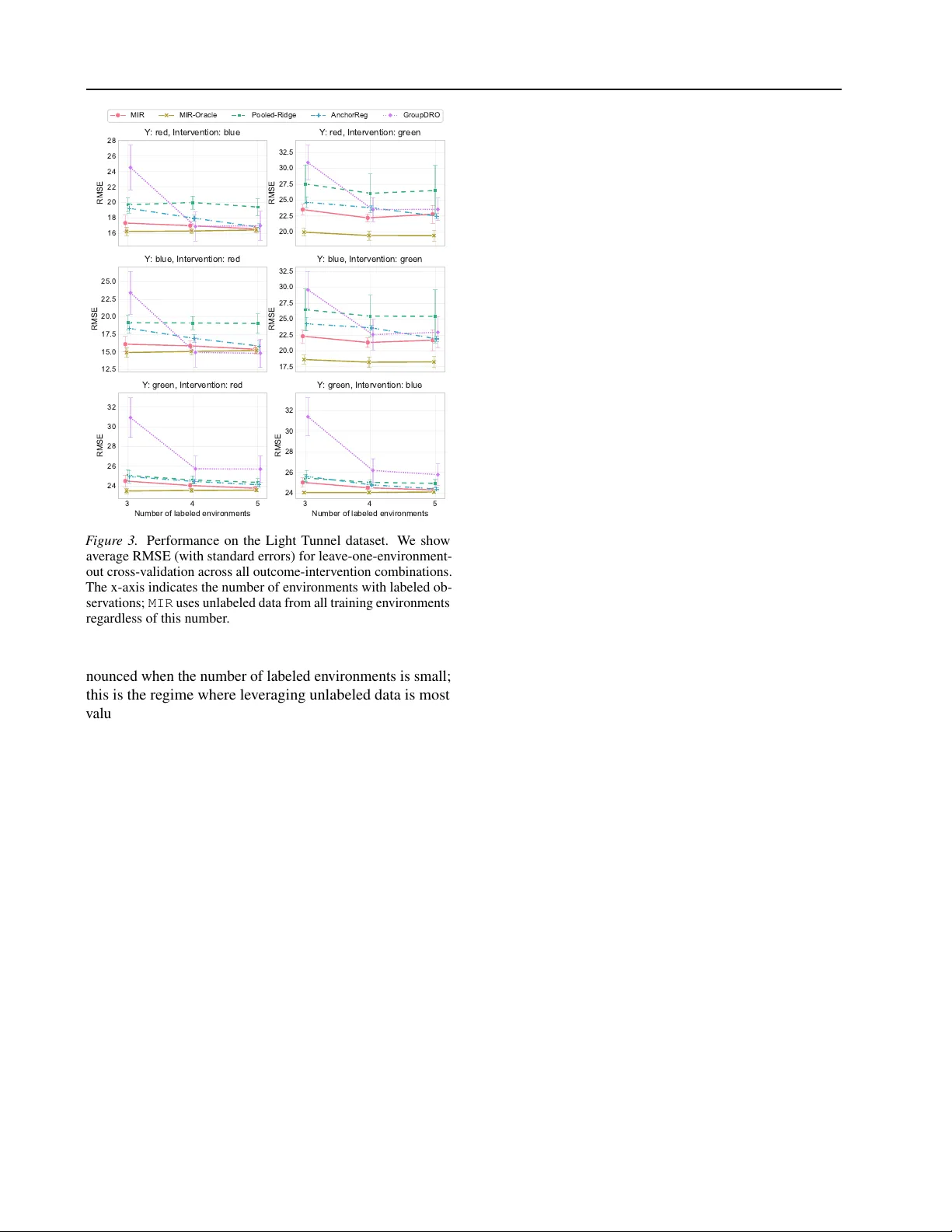
Anti-causal domain generalization: Lev eraging unlabeled data Sorawit Saengky ongam 1 Juan L. Gamella Andrew C. Miller 1 Jonas P eters 2 Nicolai Meinshausen 2 Christina Heinze-Deml 1 Abstract The problem of domain generalization concerns learning predictiv e models that are robust to distri- bution shifts when deployed in new , pre viously un- seen en vironments. Existing methods typically re- quire labeled data from multiple training en viron- ments, limiting their applicability when labeled data are scarce. In this work, we study domain generalization in an anti-causal setting, where the outcome causes the observed cov ariates. Under this structure, en vironment perturbations that af- fect the cov ariates do not propagate to the out- come, which moti v ates regularizing the model’ s sensitivity to these perturbations. Crucially , es- timating these perturbation directions does not require labels, enabling us to le verage unlabeled data from multiple en vironments. W e propose two methods that penalize the model’ s sensitivity to variations in the mean and cov ariance of the cov ariates across en vironments, respectively , and prov e that these methods have worst-case opti- mality guarantees under certain classes of en vi- ronments. Finally , we demonstrate the empirical performance of our approach on a controlled phys- ical system and a physiological signal dataset. 1. Introduction Machine learning models are often trained on data from a limited set of en vironments and subsequently deployed in new , pre viously unseen en vironments. A central challenge in this setting is domain generalization: learning predicti ve models that perform well not only on the training en viron- ments but also on nov el test en vironments that may dif fer from those seen during training ( Blanchard et al. , 2011 ; Muandet et al. , 2013 ). This challenge is particularly acute in high-stakes applications, such as healthcare, where dis- tribution shifts between hospitals, patient populations, or measurement devices can significantly impact model perfor- 1 Apple 2 ETH Zürich. Correspondence to: Sorawit Saengky- ongam . Pr eprint. F ebruary 20, 2026. mance ( Subbaswamy & Saria , 2020 ; DeGra ve et al. , 2021 ). One prominent approach to domain generalization lev erages the framework of structural causal models (SCMs; Pearl , 2009 ; Peters et al. , 2016 ) to characterize the mechanisms by which distrib utions shift across en vironments. Under this frame work, one can identify predictors that remain in- variant, and hence robust, across a class of environments implied by the underlying structural causal model. This perspectiv e has led to a variety of methods that exploit in- variance for robust prediction ( Rojas-Carulla et al. , 2018 ; Magliacane et al. , 2018 ; Arjovsk y et al. , 2019 ; Heinze-Deml & Meinshausen , 2021 ; Rothenhäusler et al. , 2021 ; Pfister et al. , 2021 ; Saengkyongam et al. , 2022 ; Shen et al. , 2026 ). Howe ver , existing methods typically require labeled data from multiple en vironments to estimate in variance proper - ties, which limits their applicability when labeled data are scarce or expensi ve to obtain. In many practical settings, unlabeled data are more abun- dant than labeled data. This motiv ates studying domain generalization in a type of semi-supervised setting: learning robust models using labeled data from only a small number of en vironments while le veraging unlabeled data from man y others. A key question we address is under which assump- tions unlabeled data can pro vide useful information about the structure of distrib ution shifts, e ven without outcome labels. This work demonstrates that this is possible under an anti-causal learning setting, where the outcome Y causes the observed predictors X . Anti-causal structures arise naturally in many applications. In healthcare, a patient’ s underlying physiological state (the outcome) often causes the observ able measurements (the predictors). In speech recognition, the spoken content (the outcome) causes the observed audio signal (the predictors). In an anti-causal setting, en vironment perturbations that only af fect the predictors X do not propagate to the out- come Y . Nevertheless, such pert urbations can induce both cov ariate and concept shifts (see Section 3 ), harming predic- tiv e performance in unseen en vironments. T o mitigate these distributional shifts, we dev elop regularization strategies that penalize sensiti vity to en vironment perturbations. Cru- cially , the perturbation directions can be estimated solely from the marginal distribution of X , without requiring la- 1 Anti-causal domain generalization: Lev eraging unlabeled data bels. W e provide theoretical guarantees showing that our regularized estimators are optimal for worst-case risk o ver a class of en vironments characterized by the directions of vari- ation in the unlabeled data, with the degree of extrapolation controlled by the regularization strength. Contributions. Our main contributions are as follo ws. 1. W e formalize an anti-causal domain generalization framew ork in a semi-supervised setting, where labeled data are a vailable from a few en vironments, and unla- beled data are av ailable from many others (Section 3 ). 2. W e propose two regularization strategies, Mean-based In v ariant Regularization (MIR) and V ariance-based In v ariant Re gularization (VIR), that exploit distribu- tional variations in the unlabeled data to encourage robustness. W e provide theoretical guarantees, sho w- ing that the regularized estimators are optimal in terms of worst-case risk ov er certain classes of environments (Section 4 ). 3. W e ev aluate our methods on two real-world datasets that naturally exhibit an anti-causal structure: a con- trolled physical system and a physiological signal dataset (Section 7 ). 2. Related W ork Our work b uilds on the literature that exploits in variance in heterogeneous data to address domain generalization; see Bühlmann ( 2020 ) for an overvie w . The concept of in vari- ant prediction ( Peters et al. , 2016 ) has been employed to identify robust (or stable) predictors across v arious settings ( Rojas-Carulla et al. , 2018 ; Heinze-Deml et al. , 2018 ; Magli- acane et al. , 2018 ; Pfister et al. , 2021 ; Heinze-Deml & Mein- shausen , 2021 ; Saengkyongam et al. , 2023 ; 2024a ). Se veral works ha ve e xtended this idea from selecting in variant pre- dictors to incorporating in variance as a re gularization term ( Arjovsk y et al. , 2019 ; Heinze-Deml & Meinshausen , 2021 ; Rothenhäusler et al. , 2021 ; Saengkyongam et al. , 2022 ; Shen et al. , 2026 ). These methods le verage causal frame works to establish theoretical guarantees for distributional rob ustness within certain classes of distributions implied by SCMs. T o the best of our kno wledge, none of the aforementioned works considers e xtracting in variance from unlabeled data. Our work utilizes assumptions from anti-causal structures, which allo w us to define an inv ariance regularization that depends solely on unlabeled observations. While Schölkopf et al. ( 2012 ) discuss the implications of anti-causal learning in a single-domain semi-supervised setting, we e xtend these ideas to semi-supervised domain generalization. Anti-causal structures were also considered in Heinze-Deml & Mein- shausen ( 2021 ); V eitch et al. ( 2021 ); Makar et al. ( 2022 ); Jiang & V eitch ( 2022 ) for domain generalization, b ut not within a semi-supervised setting. Our theoretical guarantees are closely related to those in Rothenhäusler et al. ( 2021 ) and Shen et al. ( 2026 ); ho we ver , ours differ by e xplicitly le ver - aging anti-causal assumptions to derive guarantees from in v ariance regularization that uses only unlabeled data. Another line of research focuses on explicitly optimizing worst-case group performance ( Meinshausen & Bühlmann , 2015 ; Bühlmann & Meinshausen , 2015 ; Hu et al. , 2018 ; Sagaw a et al. , 2020 ; Freni et al. , 2025 ), a framework of- ten kno wn as Group Distrib utionally Robust Optimization (GroupDR O). In GroupDR O, rob ustness is typically defined with respect to test distributions that are con vex combi- nations of training distributions, which limits the model’ s ability to extrapolate beyond the training support. In con- trast, our method considers test distributions that may lie outside the con ve x hull of the training distrib utions. Specifi- cally , we define plausible directions of extrapolation based on the directions of v ariation observed in the unlabeled data. While Krueger et al. ( 2021 ) consider extrapolation beyond con ve x combinations by optimizing the worst-case affine combination of training risks, the directions along which the model can extrapolate from the training distributions are, to our knowledge, less well-characterized. 3. Anti-causal domain generalization in a semi-supervised setting This section formalizes the setting and goal of our work. Setting 3.1 (Multi-en vironment anti-causal learning) . Let E be a collection of en vir onments, we consider the following class of structural causal models inde xed by e ∈ E : S ( e ) :      U : = ε U Y : = g 0 ( U, ε Y ) X : = f 0 ( Y , U , ε X ) + ε e , (1) e X Y U f 0 wher e X ∈ R d denotes the pr edictors, U ∈ R q denotes the unobserved confounders, Y ∈ R denotes the outcome, ( ε U , ε Y , ε X ) ar e jointly independent noise variables, and for each e ∈ E , the en vir onment perturbation ε e ∼ P e ε satisfies ε e ⊥ ⊥ ( ε U , ε Y , ε X ) . W ithout loss of gener ality , we assume that f 0 ( Y , U , ε X ) and g 0 ( U, ε Y ) have zer o mean. Remark 3.2 . (i) Although the SCM ( 1 ) imposes certain restrictions, such as the absence of a direct ef fect from e to Y , this model class can still capture non-trivial distrib ution shifts. In particular , it allows for both cov ariate shift and concept shift simultaneously: for some e 1 , e 2 ∈ E , we may have both P e 1 X  = P e 2 X and P e 1 Y | X  = P e 2 Y | X . (ii) The unobserved confounders U do not play a significant role in this model class in that removing U from the SCM ( 1 ) would not introduce any conditional independencies that could be exploited for domain generalization. 2 Anti-causal domain generalization: Lev eraging unlabeled data Notation. For each en vironment e ∈ E , we denote by P e X,Y the distribution induced by S ( e ) , and by E e and V ar e the corresponding expectation and v ariance. 3.1. Learning setting W e are giv en observations from p training en vironments E tr : = { e 1 , . . . , e p } ⊆ E , where we hav e • Labeled data from a small set of en vironments: D tr X,Y = { ( X i , Y i , E i ) } k i =1 such that ( X i , Y i ) ∼ P E i X,Y , where E i ∈ L ⊂ E tr , with L denoting the set of labeled en vironments, and k is the total number of labeled observations. W e assume { E 1 , . . . , E k } = L . • Unlabeled data from all training environments: D tr X = { ( X j , E j ) } n j =1 such that X j ∼ P E j X , where E j ∈ E tr and n is the total number of unlabeled observations, with n ≥ k (the first k observations are the X i and E i in D tr X,Y ). W e assume 1 { E 1 , . . . , E n } = E tr . Let F be a function class of interest. Our goal is to learn a predictiv e function f tr ∈ F using D tr X,Y and D tr X such that it generalizes well to an unseen test en vironment e tst ∈ E . Since we do not have additional information on the test en vironment e tst , it can be any environment in E , so possibly e tst / ∈ E tr . W e consider the worst-case risk as the objective: sup e ∈E E e [ ℓ ( f tr ( X ) , Y )] , (2) where ℓ : R × R → R is a giv en loss function. As discussed in Section 2 , the objecti ve ( 2 ) depends cru- cially on the class of en vironments E under consideration. Our approach characterizes the class E using the directions of variation observ ed in the unlabeled data. This allo ws the model to extrapolate along such directions, with the de gree of extrapolation controlled by a regularization parameter . W e now introduce our approach and formalize these ideas. 4. Data-driven r obust r egression The ke y idea of our approach is to le verage the in variance encoded in the assumed SCM ( 1 ) : the en vironment pertur- bations ε e are independent of the outcome Y , i.e., ∀ e ∈ E : ε e ⊥ ⊥ Y . (3) Intuitiv ely , if we can characterize the structure of the v ari- ations in ε e across en vironments, we can penalize models along these directions, since (i) under Setting 3.1 , such v ari- ations are the source of distributional shifts across en viron- ments, and (ii), by ( 3 ) , these v ariations carry no information about the outcome. Although ε e is not directly observ able, we show in Theorems 4.1 and 4.2 that it is possible to learn 1 This assumption ensures that we observe at least one observa- tion from each en vironment in E tr . prov ably robust models by exploiting distributional shifts estimated from unlabeled data. T o this end, we de velop reg- ularization strate gies that penalize models according to their sensitivity to these inferred shifts to promote rob ustness to en vironment shifts. In this section, we focus on the setting where F consists of linear functions and the loss ℓ is the squared error . Howe ver , these are not fundamental limitations; we discuss extensions to other loss functions and nonlinear models in Section 6 . For the remainder of this section, let E be a collection of en vironments such that { P e ε } e ∈E contains all probability dis- tributions ov er R d . W e define E tr [ · ] : = 1 |L| P e ∈L E e [ · ] as the av erage expectation ov er labeled training en vironments. 4.1. Mean-based In variant Regularization (MIR) Our first regularization strategy targets variations in the means of ε e across en vironments. Define the matrix of en vironment-specific cov ariate means as K : =  E e 1 [ X ] · · · E e p [ X ]  ∈ R d × p , which can be estimated solely from the unlabeled data. W e consider the following re gularized regression coef ficients: β MIR γ = argmin β ∈ R d E tr [( Y − β ⊤ X ) 2 ] + γ β ⊤ V ar( K ) β , (4) where V ar( K ) : = 1 p K K ⊤ −  1 p K 1 p  1 p K 1 p  ⊤ denotes the cov ariance matrix of the en vironment means and 1 p is the vector of ones. In Setting 3.1 , f 0 ( Y , U, ε X ) has zero mean, and hence E e [ X ] = E e [ ε e ] for all en vironments e ∈ E . The matrix K therefore equals K = µ tr ε : =  E [ ε e 1 ] · · · E [ ε e p ]  . Thus, the MIR regularization term β ⊤ V ar( K ) β penalizes sensitivity to mean shifts in en vironment perturbations ε e . In Theorem 4.1 belo w , we establish a dual characterization of ( 4 ) in terms of distributional rob ustness: the model coef- ficients that minimize the regularized objecti ve ( 4 ) are also optimal for the worst-case risk under a class of mean-shift perturbations, with the size of this class controlled by the regularization parameter γ . (All proofs are in Appendix A .) Theorem 4.1 (MIR Rob ustness) . Define ∆ ⋄ γ : =  A ∈ R d × d : 0 ⪯ A ⪯ γ V ar( µ tr ε )  . Under Setting 3.1 , we have β MIR γ ∈ argmin β ∈ R d sup e ∈E ⋄ γ E e [( Y − β ⊤ X ) 2 ] , wher e E ⋄ γ : = { e tst ∈ E : ∃ A ∈ ∆ ⋄ γ s.t. E e tst [ ε e ε ⊤ e ] = E tr [ ε e ε ⊤ e ] + A } . 3 Anti-causal domain generalization: Lev eraging unlabeled data 4 2 0 2 4 X 1 2.0 1.5 1.0 0.5 0.0 0.5 1.0 1.5 2.0 X 2 e 1 e 2 e 3 e 4 e 5 e 6 e 7 e 8 e 9 e t e s t OLS M I R ( = 1 0 ) M I R ( = 1 ) * t e s t T r a i n i n g e n v i r o n m e n t m e a n s : [ e i ] T e s t e n v i r o n m e n t m e a n : [ e t e s t ] V a r ( K ) ( 2 s t d ) F igur e 1. Illustration of MIR. Blue points represent the training en vironment perturbation means E [ ε e i ] , and the green star repre- sents the test environment mean. The red ellipse represents the cov ariance structure of the regularization matrix V ar( K ) , with red arrows indicating its (scaled) eigenv ectors. The annotated arro ws show the directions of the OLS and MIR solutions with different regularization strengths γ , as well as the optimal solution β ∗ test for the test en vironment e tst . Figure 1 illustrates MIR using a simulated example with p = 10 en vironments and 2-dimensional cov ariates, where one en vironment is held out as the test environment. The en vironment perturbation means { E [ ε e i ] } 10 i =1 are generated from a Gaussian distribution with a cov ariance structure such that one eigen v alue is much larger than the other . The figure shows the direction of the ordinary least squares (OLS) solution, the MIR solutions for two regularization strengths γ ∈ { 1 , 10 } , and the optimal solution β ∗ test for the test en vironment e tst . The regularization strength γ con- trols the tradeoff between the OLS solution ( γ = 0 ) and the direction of least variability . The optimal choice of γ for a giv en test en vironment depends on ho w far the test en vironment mean is from the training centroid: guarding against larger shifts requires stronger re gularization. In this example, V ar( K ) is full rank, so as γ increases, the so- lution rotates away from the direction of high variability (the first eigen vector) to ward the direction of least v ariance (the second eigen vector), and then shrinks tow ard zero as γ → ∞ . More generally , when V ar( K ) is not full rank, the solution shrinks tow ard a v ector in the null space of V ar( K ) as γ → ∞ ; this null space corresponds to the subspace of directions that are in v ariant across training en vironments. 4.2. V ariance-based In variant Regularization (VIR) Our second strategy tar gets variations in the cov ariances of ε e across en vironments. For each e ∈ E , define the co vari- ance matrix G e X : = V ar e ( X ) and the av erage cov ariance ¯ G X : = 1 p P p j =1 G e j X . W e consider the following objecti ve: β VIR γ = argmin β ∈ R d E tr [( Y − β ⊤ X ) 2 ] + γ β ⊤ 1 p p X i =1 ( G e i X − ¯ G X ) 2 ! β . (5) This regularization penalizes models that are sensitive to variations in the co variances observ ed in the unlabeled data. Analogously to the MIR case, this objectiv e admits a distri- butionally rob ust interpretation: robustness is defined with respect to shifts in the co variances of ε e , with the size of the perturbation set controlled by γ . Theorem 4.2 (VIR Robustness) . F or each e ∈ E , let G e ε : = V ar e ( ε e ) and ¯ G ε : = 1 p P p j =1 G e j ε . Define ∆ † γ : = ( A ∈ R d × d : 0 ⪯ A ⪯ γ 1 p p X i =1 ( G e i ε − ¯ G ε ) 2 ) . Under Setting 3.1 , we have β VIR γ ∈ argmin β ∈ R d sup e ∈E † γ E e [( Y − β ⊤ X ) 2 ] , wher e E † γ : = { e tst ∈ E : ∃ A ∈ ∆ † γ s.t. E e tst [ ε e ε ⊤ e ] = E tr [ ε e ε ⊤ e ] + A } . T o provide further intuition for VIR, consider the case where the cov ariance matrices of the en vironment per- turbations, { G e i ε } p i =1 , share a common eigenbasis, i.e., there exists an orthogonal matrix Q ∈ R d × d such that, for all i ∈ { 1 , . . . , p } : G e i ε = Q Λ e i Q ⊤ , where Λ e i = diag( λ e i 1 , . . . , λ e i d ) is the diagonal matrix of eigen values of G e i ε . Define the per-coordinate variance of eigen values across en vironments as σ 2 j : = 1 p p X i =1  λ e i j − ¯ λ j  2 , where ¯ λ j : = 1 p p X i =1 λ e i j . In Appendix B , we show that the VIR re gularization term simplifies to β ⊤ 1 p p X i =1 ( G e i X − ¯ G X ) 2 ! β = d X j =1 σ 2 j ( ˜ β j ) 2 , (6) where ˜ β = Q ⊤ β denotes the model coefficients projected onto the shared eigenspace. Recall that the eigen values λ e i j represent the v ariance along the j -th eigen vector direction in en vironment e i . This simplification provides a clear inter - pretation: VIR applies stronger regularization to directions along which the variances dif fer more across en vironments, thereby encouraging the model to rely on directions that are more stable. Remark 4.3 . (i) Appendix C discusses an alternati ve formu- lation of VIR that directly penalizes changes in the v ariance of predictions V ar( β ⊤ X ) across en vironments. Although this may sound intuitive, it is vulnerable to a cancellation issue: there may exist directions β that cancel out the ob- served training shifts, yielding zero penalty ev en though the direction is sensiti ve to unseen shifts. Our VIR av oids this issue; see the appendix for such an example. (ii) In practice, en vironment perturbations may affect both the means and cov ariances. W e can combine both re gularization terms in 4 Anti-causal domain generalization: Lev eraging unlabeled data a single objecti ve, as discussed in Appendix D . (iii) Under a linear model class with mean squared error loss, only the first two moments of the en vironment perturbation ε e tst af- fect the test loss. For nonlinear models and other losses (see Section 6 ), higher-moment shifts may also af fect the test loss, and extending our frame work to account for these (e.g., via a distributional metric) is a direction for future w ork. 5. Finite-sample estimators In this section, we discuss finite-sample estimators for the regularized regressions introduced in Section 4 . W e first present the population-lev el solutions and introduce plug-in estimators based on sample quantities. W e then discuss consistency of the resulting estimators. 5.1. Population-le vel solutions Consider the MIR and VIR objectiv es ( 4 ) and ( 5 ) with squared error loss. Both objecti ves are quadratic in β and ad- mit closed-form solutions. The population-le vel minimizer takes the form β γ =  E tr [ X X ⊤ ] + γ H  − 1 E tr [ X Y ] , (7) where H ∈ R d × d is a positive semi-definite matrix that encodes the directions of variation of en vironment perturba- tions ε e . Specifically , for MIR, we hav e H MIR = V ar( K ) , and for VIR, H VIR = 1 p P p i =1  G e i X − ¯ G X  2 . 5.2. Plug-in estimators Giv en labeled data D tr X,Y and unlabeled data D tr X (as defined in Section 3.1 ), we construct plug-in estimators by replacing population quantities with their sample counterparts. Let X ∈ R k × d denote the design matrix with rows X ⊤ i and Y ∈ R k denote the outcome vector , both constructed from the labeled data D tr X,Y . The plug-in estimator is ˆ β γ =  1 k X ⊤ X + γ ˆ H  − 1 1 k X ⊤ Y , (8) where ˆ H ∈ R d × d is estimated from the unlabeled data D tr X . For MIR, we use ˆ H MIR : = 1 p ˆ K ˆ K ⊤ −  1 p ˆ K 1 p  1 p ˆ K 1 p  ⊤ , (9) where ˆ K : =  ˆ µ e 1 X · · · ˆ µ e p X  ∈ R d × p and ˆ µ e i X : = 1 n i P j ∈N i X j is the sample mean of cov ariates in envi- ronment e i , with N i : = { j ∈ { 1 , . . . , n }| E j = e i } and n i : = |N i | . For VIR, we use ˆ H VIR : = 1 p p X i =1  ˆ G e i X − ˆ ¯ G X  2 , (10) where ˆ G e i X : = 1 n i P j ∈N i ( X j − ˆ µ e i X )( X j − ˆ µ e i X ) ⊤ is the sample cov ariance matrix in en vironment e i and ˆ ¯ G X : = 1 p P p i =1 ˆ G e i X is the av erage sample cov ariance across en vi- ronments. The follo wing proposition establishes that the plug-in esti- mators are consistent for the population-lev el solutions. Proposition 5.1 (Consistenc y) . Assume that E e [ ∥ X ∥ 2 2 ] < ∞ for all e ∈ E tr and E e [ Y 2 ] < ∞ for all e ∈ L , and that E tr [ X X ⊤ ] + γ H is non-singular . If k → ∞ and, for all i ∈ { 1 , . . . , p } , n i → ∞ , we have ˆ β γ p − → β γ . (11) 6. Extension: Different loss functions and nonlinear models In the previous sections, we considered the setting where F is the class of linear functions and the loss ℓ is the squared error . This section discusses e xtensions of our approach to other loss functions and to nonlinear models. 6.1. Other loss functions It is straight-forward to apply the proposed methods to other loss functions: the regularization terms (both MIR and VIR) depend solely on the unlabeled data, so the only change to the optimization problem for learning is the addition of a quadratic term. For example, for the MIR objecti ve we get argmin β ∈ R d E tr [ ℓ ( β ⊤ X, Y )] + γ 1 p β ⊤ V ar( K ) β , (12) where K =  E e 1 [ X ] · · · E e p [ X ]  is defined as before. Although the precise robustness guarantee differs from The- orem 4.1 , the intuition remains the same: we penalize β in directions that are sensiti ve to v ariation in the means of ε e . VIR can be applied analogously by replacing the MIR regularization term with that of VIR defined in ( 5 ). W e vie w this flexibility as another adv antage of our approach compared to methods that rely on residual in variance, such as Anchor regression ( Rothenhäusler et al. , 2021 ). In partic- ular , extending Anchor regression to other losses requires defining new notions of residuals with more in volv ed regu- larization terms ( K ook et al. , 2022 ). 6.2. Nonlinear models T o apply our approach to high-dimensional and/or unstruc- tured data, we adopt a representation learning perspecti ve: we first transform X via a nonlinear map ϕ and then apply a linear predictor on top of the learned representation ϕ ( X ) . The regularization is then applied to the linear predictor . This corresponds to modeling en vironment perturbations in a latent space rather than in the observed co variate space, 5 Anti-causal domain generalization: Lev eraging unlabeled data which is particularly relev ant when X consists of unstruc- tured data such as sensors, images, or text, where en viron- ment perturbations may be more meaningfully captured in a learned representation. Similar considerations have been discussed in, e.g., Rosenfeld et al. ( 2022 ); Saengkyongam et al. ( 2024b ); Šola et al. ( 2025 ); v on Kügelgen et al. ( 2025 ). Concretely , for a function class Φ , we consider the MIR objectiv e argmin ϕ ∈ Φ ,β ∈ R d ′ E tr [ ℓ ( β ⊤ ϕ ( X ) , Y )] + γ 1 p β ⊤ V ar( K ϕ ) β , (13) where K ϕ : =  E e 1 [ ϕ ( X )] · · · E e p [ ϕ ( X )]  ∈ R d ′ × p and d ′ is the dimension of the representation. Here, the regular- ization encourages the linear predictor β to be insensitiv e to en vironment perturbations in the representation space. VIR can be extended analogously by computing the variance of cov ariances in the representation space, as in ( 5 ). In many applications, the representation ϕ may be learned separately from the objecti ve ( 13 ) rather than through joint optimization. Given the recent advancements in founda- tion models that provide meaningful representations across various data modalities, our re gularization strategy can be naturally combined with these pretrained representations by fine-tuning the linear head β using the objectiv e ( 13 ) while keeping the representation ϕ fixed. W e adopt this approach in our real-world experiments (see Section 7.2 ). 7. Experiments W e ev aluate our methods on two complementary real-world datasets that naturally exhibit anti-causal structure: a con- trolled physical system and a real-w orld biomedical appli- cation. Full details on experimental setups are pro vided in Appendix E and F . 7.1. Causal Chamber: The Light T unnel The Light T unnel ( Gamella et al. , 2025 ) is a real, control- lable, optical e xperiment designed for benchmarking ma- chine learning methods. The tunnel consists of dif ferent light sources, polarizers and sensors that allow to measure and manipulate the physical v ariables of the system, while providing a causal ground truth of the effects between them. For our experiments, we focus on the main RGB light source and its ef fect on the different light-intensity sensors placed throughout the tunnel (Figure 2 ). W e select the brightness setting of one of the three color channels (red, green or blue) as the outcome Y ∈ R and use the measurements produced by the sensors as the predictors X ∈ R 6 . W e create six environments e ∈ E by performing inter- ventions on another color channel by shifting the uniform distribution from which their brightness settings are sam- Light source Light sensor Light sensor Light sensor red green blue ir_1 vis_1 ir_2 vis_2 ir_3 vis_3 M M M M M M I I I F igur e 2. Diagram of the light tunnel and the subset of variables used in our experiment: the outcomes or intervention tar gets red , green and blue , and the light-intensity measurements ir_1 , vis_1 , . . . , vis_3 used as predictors. Figure adapted from Gamella et al. ( 2025 ), licensed under CC BY 4.0. pled. By construction, these interventions induce only mean shifts in the covariate distribution, making this a suitable setting to ev aluate MIR (VIR is e valuated in another e xperi- ment, see Section 7.2 ). W e repeat the overall experiment six times by considering each outcome-intervention pair (e.g., outcome red with intervention on blue), resulting in a total of six experiments with six distinct en vironments each. Baselines. W e compare the following methods: (i) Pooled-Ridge : Ridge regression pooling data across all training en vironments. (ii) MIR : Our mean-based in- variant regularization, with the regularization parameter selected via leav e-one-en vironment-out cross-validation on the training en vironments. (iii) MIR-Oracle : Our method with the regularization parameter tuned on the test envi- ronment, serving as an upper bound on MIR performance. (iv) AnchorReg : Anchor regression ( Rothenhäusler et al. , 2021 ). (v) GroupDRO : Group distrib utionally robust opti- mization ( Sagaw a et al. , 2020 ). Evaluation setup. For each outcome-intervention pair, we adopt a leav e-one-en vironment-out ev aluation protocol: one environment is held out for testing while models are trained on the remaining fi ve en vironments. T o e valuate the semi-supervised setting, we vary the number of training en vironments that have labeled data from 3 to 5, while using unlabeled data from all training en vironments for MIR . Predicti ve performance is assessed using root mean squared error (RMSE) on the held-out en vironment (Figure 3 ). Results. Figure 3 sho ws the results across all outcome- intervention pairs. Pooled-Ridge performs poorly when generalizing to unseen en vironments, particularly when few labeled en vironments are av ailable. This indicates that, in this experiment, standard empirical risk minimization is not sufficient to generalize to unseen environments. MIR achiev es lo wer or comparable error to all baselines across all settings. The improvement over baselines is most pro- 6 Anti-causal domain generalization: Lev eraging unlabeled data 16 18 20 22 24 26 28 RMSE Y : red, Intervention: blue 20.0 22.5 25.0 27.5 30.0 32.5 RMSE Y : red, Intervention: green 12.5 15.0 17.5 20.0 22.5 25.0 RMSE Y : blue, Intervention: red 17.5 20.0 22.5 25.0 27.5 30.0 32.5 RMSE Y : blue, Intervention: green 3 4 5 Number of labeled environments 24 26 28 30 32 RMSE Y : green, Intervention: red 3 4 5 Number of labeled environments 24 26 28 30 32 RMSE Y : green, Intervention: blue MIR MIR-Oracle Pooled-Ridge AnchorReg GroupDRO F igur e 3. Performance on the Light Tunnel dataset. W e show av erage RMSE (with standard errors) for leav e-one-en vironment- out cross-validation across all outcome-intervention combinations. The x-axis indicates the number of en vironments with labeled ob- servations; MIR uses unlabeled data from all training environments regardless of this number . nounced when the number of labeled en vironments is small; this is the re gime where le veraging unlabeled data is most val uable. Comparing MIR and MIR-Oracle suggests that leav e-one-en vironment-out cross-validation often yields re g- ularization parameters that are close to being optimal but also that there are settings which carry potential for im- prov ed ways of choosing the regularization parameter . 7.2. V italDB: Strok e V olume Prediction fr om Arterial W av eforms As a real-world application in the healthcare domain, we apply our approach to predicting strok e volume from arte- rial pressure wa veform (APW) signals using data from the V italDB dataset ( Lee et al. , 2022 ). Predicting stroke v ol- ume for unseen subjects is challenging due to pronounced between-subject v ariability that induces distribution shifts. This task exhibits a natural anti-causal structure: the stroke volume Y causally influences the observed arterial pressure wa veform X , while unobserved physiological factors U may affect both. Prepr ocessing. Absolute prediction of hemodynamic pa- rameters from arterial wav eforms typically requires subject- specific calibration, such as thermodilution, to establish a baseline reference point ( Saugel et al. , 2021 ; Manduchi et al. , 2024 ). W ithout such calibration, dif ferences in base- line physiology across subjects (e.g., due to age, v ascular stiffness, or body composition) may confound the relation- ship between waveform features and absolute hemodynamic values. In the context of Setting 3.1 , these baseline dif fer- ences correspond to direct shifts from E to U (or Y ), which would violate the assumption that the en vironment does not affect Y (through U ). W e therefore focus on predicting vari ations in stroke v olume rather than absolute v alues. Con- cretely , we consider a subject-centered approach where both predictors and outcomes are mean-centered within each sub- ject. T o obtain absolute predictions, one can combine our predictions with a baseline reference point from standard calibration procedures ( Saugel et al. , 2021 ). In this subject- centered setting, mean shifts are remo ved by construction, making our V ariance-based In variant Re gularization (VIR) the appropriate method to address the remaining covariance shifts in X across subjects. Featur e representation. F ollowing the formulation in Section 6.2 , we extract 140-dimensional embeddings from arterial pressure wav eforms using a pretrained con volu- tional neural network dev eloped by Manduchi et al. ( 2024 ); Palumbo et al. ( 2025 ). This model was trained using a neural posterior estimator ( Lueckmann et al. , 2017 ) on synthetic data generated from the OpenBF cardiov ascular simula- tor ( Benemerito et al. , 2024 ), which models hemodynamics based on physiological parameters. The learned embeddings capture physiologically relev ant features of the arterial pres- sure wa veform without requiring labeled clinical data for training ( Manduchi et al. , 2024 ; Palumbo et al. , 2025 ). This pretrained representation serves as the fix ed nonlinear map ϕ , and we apply all considered methods to the linear head on top of these embeddings. Concretely , we have: • X ∈ R 140 : APW embeddings (subject-centered) • Y ∈ R : Stroke v olume variations (subject-centered) • e ∈ E : Indi vidual subjects ( n = 128 subjects) Baselines. W e consider the same baselines as in Sec- tion 7.1 , with the exception of AnchorReg . Since the subject-centered preprocessing remov es all mean shifts by construction, the Anchor re gression regularization term is zero by design. Evaluation setup. W e treat each subject as a distinct en- vironment and adopt a leave-one-subject-out e valuation pro- tocol: one subject is held out for testing while models are trained on the remaining subjects. T o e valuate the semi- supervised setting, we vary the number of training subjects with labeled observations from 20 to 127, while using un- labeled data from all training subjects for VIR. Predictiv e 7 Anti-causal domain generalization: Lev eraging unlabeled data 0% 10% 20% 30% 40% 50% 60% 70% 80% 90% 100% Quantile 2 4 6 8 nMSE Above Quantile VIR VIR-Oracle Pooled-Ridge GroupDRO (a) Robustness analysis VIR VIR-Oracle Pooled-Ridge GroupDRO 0.4 0.2 0.0 0.2 0.4 0.6 0.8 1.0 Spearman Correlation (b) T racking performance F igur e 4. Performance on V italDB dataset when all 128 training subjects hav e labeled data. (a) CV aR (av erage nMSE for subjects whose errors are abov e a giv en quantile) as a function of quantile threshold. (b) Distrib ution of per-subject Spearman’ s correlations between predicted and true stroke v olume v ariations. VIR achiev es improv ed rob ustness, especially on worse-performing subjects, while maintaining tracking performance comparable to baselines. performance is assessed on the held-out subject using nor- malized mean squared error (nMSE), defined as the mean squared error di vided by the variance of the subject’ s out- come. This normalization ensures that subjects with differ - ent outcome variability contrib ute equally to the ev aluation; otherwise, subjects with larger stroke volume v ariations would dominate the aggre gate error . T o assess robustness, we report the conditional value at risk (CV aR), computed as the a verage nMSE for subjects above a giv en quantile threshold of the nMSE distribution, where higher quantiles correspond to worse-performing subjects. Additionally , we report Spearman’ s correlation between predicted and true stroke v olume variations to e valuate tracking performance (i.e., how well predictions follo w the temporal v ariations within a subject regardless of magnitude). Results. Figure 4a sho ws the robustness analysis when all 128 training subjects have labeled data, where each point represents the CV aR at a given quantile threshold. The Pooled-Ridge baseline exhibits poor robustness; its error increases substantially for more difficult sub- jects. GroupDRO improv es o ver Pooled-Ridge but still shows relativ ely poor performance on dif ficult subjects. In contrast, VIR achiev es lower nMSE across all quantiles. 20 50 80 127 Number of labeled environments 0.5 0.6 0.7 0.8 0.9 1.0 A verage nMSE VIR VIR-Oracle Pooled-Ridge GroupDRO F igur e 5. Performance on V italDB dataset as a function of the number of labeled en vironments. VIR improv es ov er baselines across all settings. The improvement is most pronounced when few labeled en vironments are av ailable. Since dif ficult subjects correspond to those with larger dis- tributional shifts, this is consistent with VIR’ s objecti ve of penalizing sensitivity to such shifts. A natural follow-up question is whether these robustness gains compromise tracking performance. Regularization could improv e worst-case nMSE simply by shrinking pre- dictions to ward zero rather than by learning rob ust structure. Figure 4b sho ws the distribution of per-subject Spearman correlations. VIR achiev es median correlation comparable to Pooled-Ridge , with both methods centered around 0.8. The rob ustness improvements therefore do not come at the cost of tracking accuracy . Lastly , Figure 5 sho ws av erage nMSE as a function of the number of labeled en vironments. VIR yields lower errors than Pooled-Ridge and GroupDRO in all settings. The improv ement is most pronounced when the number of la- beled en vironments is small: in this regime, the regulariza- tion matrix estimated from unlabeled data provides informa- tion on en vironment perturbations that may not be possible to infer from labeled data alone. When all training subjects hav e labeled data, VIR still sho ws improv ements over the baselines, which suggests that our approach yields benefits beyond the semi-supervised setting. Ho wev er , ho w to best tune the hyperparameter γ remains an open problem, as the gap between VIR and VIR-Oracle remains significant. 8. Conclusion W e presented a frame work for anti-causal learning that le ver- ages unlabeled multi-en vironment data to improv e domain generalization. Our proposed methods have worst-case op- timality guarantees and admit closed-form estimators. Ex- periments on a real-world physical system and a biomedical application demonstrate the ef fectiv eness of our approach. This work opens avenues for improving domain general- ization in settings where obtaining labels from multiple en vironments is dif ficult but unlabeled data are ab undant. 8 Anti-causal domain generalization: Lev eraging unlabeled data Impact Statement This paper presents work tow ards making machine learning models more robust and safe for deployment under distribu- tion shift. By dev eloping methods that le verage unlabeled data to improve worst-case performance in unseen envi- ronments, our contributions ha ve potential positi ve societal impact in applications where reliability is critical. W e do not foresee ethical concerns with this work. The methods are general-purpose tools for robust prediction, the datasets used in all experiments hav e been peer -revie wed and are publicly av ailable, and the computational require- ments are minimal. References Arjovsk y , M., Bottou, L., Gulrajani, I., and Lopez- Paz, D. In v ariant risk minimization. arXiv preprint arXiv:1907.02893 , 2019. Benemerito, I., Melis, A., W ehenkel, A., and Marzo, A. openbf: an open-source finite volume 1d blood flow solver . Physiological Measurement , 2024. Blanchard, G., Lee, G., and Scott, C. Generalizing from sev eral related classification tasks to a new unlabeled sample. In Advances in neural information pr ocessing systems , volume 24, 2011. Bühlmann, P . Inv ariance, causality and rob ustness. Statisti- cal Science , 35(3):404–426, 2020. Bühlmann, P . and Meinshausen, N. Magging: maximin aggregation for inhomogeneous lar ge-scale data. Pr o- ceedings of the IEEE , 104(1):126–135, 2015. DeGrav e, A. J., Janizek, J. D., and Lee, S.-I. Ai for radio- graphic covid-19 detection selects shortcuts ov er signal. Natur e Machine Intellig ence , 3(7):610–619, 2021. Freni, F ., Fries, A., Kühne, L., Reichstein, M., and Peters, J. Maximum risk minimization with random forests. arXiv pr eprint arXiv:2512.10445 , 2025. Gamella, J. L., Peters, J., and Bühlmann, P . Causal cham- bers as a real-world physical testbed for ai methodology . Natur e Machine Intellig ence , 7(1):107–118, 2025. Heinze-Deml, C. and Meinshausen, N. Conditional v ariance penalties and domain shift rob ustness. Machine Learning , 110(2):303–348, 2021. Heinze-Deml, C., Peters, J., and Meinshausen, N. In variant causal prediction for nonlinear models. J ournal of Causal Infer ence , 6(2):1–35, 2018. Hu, W ., Niu, G., Sato, I., and Sugiyama, M. Does distribu- tionally rob ust supervised learning gi ve rob ust classifiers? In International Confer ence on Machine Learning , pp. 2029–2037. PMLR, 2018. Jiang, Y . and V eitch, V . In variant and transportable represen- tations for anti-causal domain shifts. Advances in Neural Information Pr ocessing Systems , 35:20782–20794, 2022. K ook, L., Sick, B., and Bühlmann, P . Distributional anchor regression. Statistics and Computing , 32(3):39, 2022. Krueger , D., Caballero, E., Jacobsen, J.-H., Zhang, A., Bi- nas, J., Zhang, D., Le Priol, R., and Courville, A. Out-of- distribution generalization via risk extrapolation (rex). In International confer ence on machine learning , pp. 5815– 5826. PMLR, 2021. Lee, H.-C., Park, Y ., Y oon, S. B., Y ang, S. M., Park, D., and Jung, C.-W . V italdb, a high-fidelity multi-parameter vital signs database in surgical patients. Scientific Data , 9(1): 279, 2022. Lueckmann, J.-M., Goncalves, P . J., Bassetto, G., Öcal, K., Nonnenmacher , M., and Macke, J. H. Flexible statistical inference for mechanistic models of neural dynamics. Advances in neural information pr ocessing systems , 30, 2017. Magliacane, S., V an Ommen, T ., Claassen, T ., Bongers, S., V ersteeg, P ., and Mooij, J. M. Domain adaptation by using causal inference to predict in variant conditional distributions. Advances in neural information pr ocessing systems , 31, 2018. Makar , M., Packer , B., Moldov an, D., Blalock, D., Halpern, Y ., and D’Amour , A. Causally motiv ated shortcut remov al using auxiliary labels. In International Confer ence on Artificial Intelligence and Statistics , pp. 739–766. PMLR, 2022. Manduchi, L., W ehenkel, A., Behrmann, J., Pegolotti, L., Miller , A. C., Sener , O., Cuturi, M., Sapiro, G., and Jacobsen, J.-H. Lev eraging cardio vascular simulations for in-viv o prediction of cardiac biomarkers. arXiv pr eprint arXiv:2412.17542 , 2024. Meinshausen, N. and Bühlmann, P . Maximin ef fects in inhomogeneous large-scale data. Annals of Statistics , 43 (4):1801–1830, 2015. Muandet, K., Balduzzi, D., and Schölkopf, B. Domain generalization via inv ariant feature representation. In Pr oceedings of the 30th International Confer ence on Ma- chine Learning , pp. 10–18. PMLR, 2013. 9 Anti-causal domain generalization: Lev eraging unlabeled data Palumbo, E., Saengk yongam, S., Cerv era, M. R., Behrmann, J., Miller , A. C., Sapiro, G., Heinze-Deml, C., and W e- henkel, A. Hybrid modeling of photoplethysmography for non-in vasi ve monitoring of cardio v ascular parameters. arXiv pr eprint arXiv:2511.14452 , 2025. Pearl, J. Causality: Models, Reasoning, and Infer ence . Cam- bridge University Press, New Y ork, USA, 2nd edition, 2009. Peters, J., Bühlmann, P ., and Meinshausen, N. Causal in- ference by using in variant prediction: identification and confidence interv als. Journal of the Royal Statistical So- ciety . Series B (Statistical Methodology) , pp. 947–1012, 2016. Pfister , N., Williams, E. G., Peters, J., Aebersold, R., and Bühlmann, P . Stabilizing variable selection and re gres- sion. The Annals of Applied Statistics , 15(3):1220–1246, 2021. Rojas-Carulla, M., Schölkopf, B., T urner , R., and Peters, J. In variant models for causal transfer learning. The Journal of Machine Learning Resear ch , 19(1):1309–1342, 2018. Rosenfeld, E., Ravikumar , P ., and Risteski, A. Domain- adjusted regression or: Erm may already learn features sufficient for out-of-distrib ution generalization. arXiv pr eprint arXiv:2202.06856 , 2022. Rothenhäusler , D., Meinshausen, N., Bühlmann, P ., and Peters, J. Anchor regression: Heterogeneous data meet causality . Journal of the Royal Statistical Society: Series B (Statistical Methodology) , 83(2):215–246, 2021. Saengkyongam, S., Henckel, L., Pfister , N., and Peters, J. Exploiting independent instruments: Identification and distribution generalization. In International Confer ence on Machine Learning , pp. 18935–18958. PMLR, 2022. Saengkyongam, S., Thams, N., Peters, J., and Pfister , N. In v ariant policy learning: A causal perspecti ve. IEEE transactions on pattern analysis and machine intelligence , 45(7):8606–8620, 2023. Saengkyongam, S., Pfister , N., Klasnja, P ., Murphy , S., and Peters, J. Effect-in variant mechanisms for policy generalization. Journal of Machine Learning Resear ch , 25(34):1–36, 2024a. Saengkyongam, S., Rosenfeld, E., Ravikumar , P . K., Pfister , N., and Peters, J. Identifying representations for inter- vention extrapolation. In International Confer ence on Learning Repr esentations , 2024b. Sagaw a, S., K oh, P . W ., Hashimoto, T . B., and Liang, P . Distributionally rob ust neural networks for group shifts: On the importance of re gularization for worst-case gen- eralization. In International Confer ence on Learning Repr esentations , 2020. Saugel, B., K ouz, K., Scheeren, T . W ., Greiwe, G., Hoppe, P ., Romagnoli, S., and de Backer , D. Cardiac output estimation using pulse wav e analysis—physiology , al- gorithms, and technologies: a narrativ e re view . British journal of anaesthesia , 126(1):67–76, 2021. Schölkopf, B., Janzing, D., Peters, J., Sgouritsa, E., Zhang, K., and Mooij, J. On causal and anticausal learning. Pr oceedings of the 29th International Confer ence on Ma- chine Learning , pp. 459–466, 2012. Shen, X., Bühlmann, P ., and T aeb, A. Causality-oriented robustness: exploiting general noise interv entions in lin- ear structural causal models. Journal of the American Statistical Association (to appear) , pp. 1–20, 2026. Šola, M., Bühlmann, P ., and Shen, X. Causality-inspired ro- bustness for nonlinear models via representation learning. arXiv pr eprint arXiv:2505.12868 , 2025. Subbaswamy , A. and Saria, S. From de velopment to deploy- ment: dataset shift, causality , and shift-stable models in health ai. Biostatistics , 21(2):345–352, 2020. V eitch, V ., D’Amour , A., Y adlo wsky , S., and Eisenstein, J. Counterfactual in variance to spurious correlations in text classification. Advances in neur al information pr ocessing systems , 34:16196–16208, 2021. von Kügelgen, J., Ketterer , J., Shen, X., Meinshausen, N., and Peters, J. Representation learning for dis- tributional perturbation extrapolation. arXiv preprint arXiv:2504.18522 , 2025. 10 Anti-causal domain generalization: Lev eraging unlabeled data A. Proofs Throughout this section, we work under Setting 3.1 . W e use the notation introduced in Section 4 . For the proofs, we additionally define for an y en vironment e ∈ E : • M e ε : = E [ ε e ε ⊤ e ] , the second moment matrix of the perturbation, • ¯ M ε : = 1 |L| P e ∈L M e ε , the av erage second moment across labeled en vironments. A.1. Preliminary Lemma The following lemma provides a decomposition of the mean squared error that separates en vironment-in v ariant and en vironment-specific components. Lemma A.1 (MSE Decomposition) . Under Setting 3.1 , for any β ∈ R d and any en vir onment e ∈ E , E e [( Y − β ⊤ X ) 2 ] = R 0 ( β ) + β ⊤ M e ε β , wher e R 0 ( β ) : = E [( Y − β ⊤ f 0 ( Y , U, ε X )) 2 ] does not depend on the en vir onment e . Pr oof. Under Setting 3.1 , we hav e X = f 0 ( Y , U, ε X ) + ε e . Define Z : = f 0 ( Y , U, ε X ) . Expanding the squared error: E e [( Y − β ⊤ X ) 2 ] = E [( Y − β ⊤ Z − β ⊤ ε e ) 2 ] = E [( Y − β ⊤ Z ) 2 ] | {z } (I) − 2 E [( Y − β ⊤ Z ) · β ⊤ ε e ] | {z } (II) + E [( β ⊤ ε e ) 2 ] | {z } (III) . W e analyze each term separately . T erm (I): This equals R 0 ( β ) by definition. It depends only on the joint distrib ution of ( ε Y , ε U , ε X ) , which is in variant across en vironments by Setting 3.1 . T erm (II): By the independence of ε e from ( ε Y , ε U , ε X ) stated in Setting 3.1 , we can factorize the expectation: E [( Y − β ⊤ Z ) · β ⊤ ε e ] = E [ Y − β ⊤ Z ] · E [ β ⊤ ε e ] . By Setting 3.1 , E [ Z ] = E [ f 0 ( Y , U, ε X )] = 0 and E [ Y ] = E [ g 0 ( U, ε Y )] = 0 . Therefore, E [ Y − β ⊤ Z ] = 0 , and T erm (II) vanishes. T erm (III): This equals E [( β ⊤ ε e ) 2 ] = β ⊤ E [ ε e ε ⊤ e ] β = β ⊤ M e ε β . Combining these results: E e [( Y − β ⊤ X ) 2 ] = R 0 ( β ) + β ⊤ M e ε β . □ A.2. Proof of Theor em 4.1 Recall that µ tr ε : =  E [ ε e 1 ] · · · E [ ε e p ]  ∈ R d × p denotes the matrix of perturbation means across all training en vironments E tr = { e 1 , . . . , e p } . Pr oof. The proof proceeds in three steps. Step 1: Express the MSE for en vir onments in E ⋄ γ . By Lemma A.1 , for any en vironment e ∈ E , E e [( Y − β ⊤ X ) 2 ] = R 0 ( β ) + β ⊤ M e ε β . Step 2: Compute the supremum o ver E ⋄ γ . W e claim that sup e ∈E ⋄ γ β ⊤ M e ε β = β ⊤ ¯ M ε β + sup A ∈ ∆ ⋄ γ β ⊤ Aβ . (14) 11 Anti-causal domain generalization: Lev eraging unlabeled data T o establish ( 14 ), we show that { M e ε − ¯ M ε : e ∈ E ⋄ γ } = ∆ ⋄ γ : • By definition of E ⋄ γ , for ev ery e ∈ E ⋄ γ , we hav e M e ε − ¯ M ε ∈ ∆ ⋄ γ . • Con versely , for ev ery A ∈ ∆ ⋄ γ , the matrix ¯ M ε + A is positi ve semi-definite (as the sum of tw o positiv e semi-definite matrices). Since E contains all en vironments whose perturbation distribution ranges o ver all probability distrib utions on R d , there exists e ∈ E with M e ε = ¯ M ε + A . This e belongs to E ⋄ γ by definition, and hence A ∈ { M e ε − ¯ M ε : e ∈ E ⋄ γ } . This set equality implies: sup e ∈E ⋄ γ β ⊤ M e ε β = sup e ∈E ⋄ γ β ⊤ ( ¯ M ε + ( M e ε − ¯ M ε )) β = β ⊤ ¯ M ε β + sup e ∈E ⋄ γ β ⊤ ( M e ε − ¯ M ε ) β = β ⊤ ¯ M ε β + sup A ∈ ∆ ⋄ γ β ⊤ Aβ , where the last equality uses { M e ε − ¯ M ε : e ∈ E ⋄ γ } = ∆ ⋄ γ . Therefore, sup e ∈E ⋄ γ E e [( Y − β ⊤ X ) 2 ] = R 0 ( β ) + sup e ∈E ⋄ γ β ⊤ M e ε β = R 0 ( β ) + β ⊤ ¯ M ε β + sup A ∈ ∆ ⋄ γ β ⊤ Aβ . W e now e valuate sup A ∈ ∆ ⋄ γ β ⊤ Aβ . Upper bound: For any A ∈ ∆ ⋄ γ , the constraint 0 ⪯ A ⪯ γ V ar( µ tr ε ) implies β ⊤ Aβ ≤ γ β ⊤ V ar( µ tr ε ) β . Attainability: Define A ∗ : = γ V ar( µ tr ε ) . W e verify that A ∗ ∈ ∆ ⋄ γ : • A ∗ is symmetric since V ar( µ tr ε ) is a cov ariance matrix. • A ∗ is positiv e semi-definite since V ar( µ tr ε ) is positiv e semi-definite. • A ∗ ⪯ γ V ar( µ tr ε ) holds with equality . Therefore, A ∗ ∈ ∆ ⋄ γ , and the upper bound is achiev ed: sup A ∈ ∆ ⋄ γ β ⊤ Aβ = γ β ⊤ V ar( µ tr ε ) β . (15) Combining the abov e, sup e ∈E ⋄ γ E e [( Y − β ⊤ X ) 2 ] = R 0 ( β ) + β ⊤ ¯ M ε β + γ β ⊤ V ar( µ tr ε ) β . (16) Step 3: Relate to the MIR objective. W e compute the average training MSE o ver labeled en vironments. By Lemma A.1 , E tr [( Y − β ⊤ X ) 2 ] = 1 |L| X e ∈L E e [( Y − β ⊤ X ) 2 ] = 1 |L| X e ∈L  R 0 ( β ) + β ⊤ M e ε β  = R 0 ( β ) + β ⊤ ¯ M ε β . (17) Substituting ( 17 ) into ( 16 ), sup e ∈E ⋄ γ E e [( Y − β ⊤ X ) 2 ] = E tr [( Y − β ⊤ X ) 2 ] + γ β ⊤ V ar( µ tr ε ) β . (18) 12 Anti-causal domain generalization: Lev eraging unlabeled data Finally , we show that K = µ tr ε . Under Setting 3.1 , for each training environment e i , E e i [ X ] = E [ f 0 ( Y , U, ε X ) + ε e i ] = E [ f 0 ( Y , U, ε X )] + E [ ε e i ] . Since E [ f 0 ( Y , U, ε X )] = 0 by Setting 3.1 , we hav e E e i [ X ] = E [ ε e i ] . Therefore, K =  E e 1 [ X ] · · · E e p [ X ]  =  E [ ε e 1 ] · · · E [ ε e p ]  = µ tr ε . Since K = µ tr ε , we hav e V ar( K ) = V ar( µ tr ε ) . Substituting into ( 18 ), sup e ∈E ⋄ γ E e [( Y − β ⊤ X ) 2 ] = E tr [( Y − β ⊤ X ) 2 ] + γ β ⊤ V ar( K ) β . The right-hand side is precisely the MIR objectiv e ( 4 ) . Since the equality holds for all β ∈ R d , minimizing ov er β on both sides yields β MIR γ = argmin β ∈ R d  E tr [( Y − β ⊤ X ) 2 ] + γ β ⊤ V ar( K ) β  = argmin β ∈ R d sup e ∈E ⋄ γ E e [( Y − β ⊤ X ) 2 ] . □ A.3. Proof of Theor em 4.2 Recall the notation from Section 4 : for each en vironment e i ∈ E tr , G e i X denotes the cov ariance matrix of X , G e i ε denotes the cov ariance matrix of ε e i , and ¯ G X : = 1 p P p i =1 G e i X and ¯ G ε : = 1 p P p i =1 G e i ε denote their averages across all training en vironments. Lemma A.2. The matrix V ε : = 1 p P p i =1 ( G e i X − ¯ G X ) 2 is symmetric and positive semi-definite. Pr oof. Each G e i X − ¯ G X is symmetric (as a dif f erence of covariance matrices). The square of a symmetric matrix is symmetric and positiv e semi-definite. The sum of positive semi-definite matrices is positi ve semi-definite. □ Pr oof of Theorem 4.2 . The proof follows the same structure as the proof of Theorem 4.1 . Step 1: Express the MSE for en vir onments in E † γ . By Lemma A.1 , for any en vironment e ∈ E , E e [( Y − β ⊤ X ) 2 ] = R 0 ( β ) + β ⊤ M e ε β . Step 2: Compute the supremum o ver E † γ . W e claim that sup e ∈E † γ β ⊤ M e ε β = β ⊤ ¯ M ε β + sup A ∈ ∆ † γ β ⊤ Aβ . (19) T o establish ( 19 ), we show that { M e ε − ¯ M ε : e ∈ E † γ } = ∆ † γ : • By definition of E † γ , for ev ery e ∈ E † γ , we hav e M e ε − ¯ M ε ∈ ∆ † γ . • Con versely , for ev ery A ∈ ∆ † γ , the matrix ¯ M ε + A is positi ve semi-definite (as the sum of tw o positiv e semi-definite matrices). Since E contains all en vironments whose perturbation distribution ranges o ver all probability distrib utions on R d , there exists e ∈ E with M e ε = ¯ M ε + A . This e belongs to E † γ by definition, and hence A ∈ { M e ε − ¯ M ε : e ∈ E † γ } . This set equality implies: sup e ∈E † γ β ⊤ M e ε β = sup e ∈E † γ β ⊤ ( ¯ M ε + ( M e ε − ¯ M ε )) β = β ⊤ ¯ M ε β + sup e ∈E † γ β ⊤ ( M e ε − ¯ M ε ) β = β ⊤ ¯ M ε β + sup A ∈ ∆ † γ β ⊤ Aβ , 13 Anti-causal domain generalization: Lev eraging unlabeled data where the last equality uses { M e ε − ¯ M ε : e ∈ E † γ } = ∆ † γ . Therefore, sup e ∈E † γ E e [( Y − β ⊤ X ) 2 ] = R 0 ( β ) + sup e ∈E † γ β ⊤ M e ε β = R 0 ( β ) + β ⊤ ¯ M ε β + sup A ∈ ∆ † γ β ⊤ Aβ . W e now e valuate sup A ∈ ∆ † γ β ⊤ Aβ . Upper bound: For any A ∈ ∆ † γ , the constraint 0 ⪯ A ⪯ γ V ε implies β ⊤ Aβ ≤ γ β ⊤ V ε β . Attainability: Define A ∗ : = γ V ε . By Lemma A.2 , V ε is symmetric and positive semi-definite, so A ∗ is as well. The constraint A ∗ ⪯ γ V ε holds with equality . Therefore, A ∗ ∈ ∆ † γ , and the upper bound is achiev ed: sup A ∈ ∆ † γ β ⊤ Aβ = γ β ⊤ V ε β . (20) Combining the abov e, sup e ∈E † γ E e [( Y − β ⊤ X ) 2 ] = R 0 ( β ) + β ⊤ ¯ M ε β + γ β ⊤ V ε β . (21) Step 3: Relate to the VIR objective. By the same calculation as in ( 17 ), E tr [( Y − β ⊤ X ) 2 ] = 1 |L| X e ∈L E e [( Y − β ⊤ X ) 2 ] = R 0 ( β ) + β ⊤ ¯ M ε β . (22) Substituting ( 22 ) into ( 21 ), sup e ∈E † γ E e [( Y − β ⊤ X ) 2 ] = E tr [( Y − β ⊤ X ) 2 ] + γ β ⊤ V ε β . (23) It remains to show that V ε = 1 p P p i =1 ( G e i X − ¯ G X ) 2 . Under Setting 3.1 , we have X = Z + ε e where Z : = f 0 ( Y , U, ε X ) . Since ε e is independent of ( ε Y , ε U , ε X ) , the cov ariance of X in en vironment e i decomposes as: G e i X = G Z + G e i ε , (24) where G Z : = V ar( Z ) denotes the cov ariance of Z , which does not depend on the environment. T aking the average across all training en vironments, ¯ G X = 1 p p X i =1 G e i X = G Z + ¯ G ε . Therefore, for each training en vironment e i , G e i X − ¯ G X = G e i ε − ¯ G ε . (25) Consequently , 1 p p X i =1 ( G e i X − ¯ G X ) 2 = 1 p p X i =1 ( G e i ε − ¯ G ε ) 2 = V ε . (26) 14 Anti-causal domain generalization: Lev eraging unlabeled data Substituting into ( 23 ), sup e ∈E † γ E e [( Y − β ⊤ X ) 2 ] = E tr [( Y − β ⊤ X ) 2 ] + γ β ⊤ 1 p p X i =1 ( G e i X − ¯ G X ) 2 ! β . The right-hand side is precisely the VIR objecti ve ( 5 ) . Since the equality holds for all β ∈ R d , minimizing ov er β on both sides yields β VIR γ = argmin β ∈ R d ( E tr [( Y − β ⊤ X ) 2 ] + γ β ⊤ 1 p p X i =1 ( G e i X − ¯ G X ) 2 ! β ) = argmin β ∈ R d sup e ∈E † γ E e [( Y − β ⊤ X ) 2 ] . □ A.4. Proof of Pr oposition 5.1 Pr oof. Recall the assumptions of Proposition 5.1 : (i) E e [ ∥ X ∥ 2 2 ] < ∞ for all e ∈ E tr , (ii) E e [ Y 2 ] < ∞ for all e ∈ L , (iii) E tr [ X X ⊤ ] + γ H is non-singular . For each labeled en vironment e ∈ L , let k e denote the number of samples from en vironment e , so that k = P e ∈L k e . W e assume balanced sampling, i.e., k e /k → 1 / |L| for each e ∈ L (the proof for unbalanced sampling follows analogously with E tr [ · ] defined as the corresponding weighted av erage). The finite-sample estimator admits the closed-form solution: ˆ β γ =  1 k X ⊤ X + γ ˆ H  − 1  1 k X ⊤ Y  . W e establish the conv ergence in probability of each component. 1. Labeled data conv ergence: The sample second moment from the labeled data can be written as: 1 k X ⊤ X = X e ∈L k e k 1 k e X i : E i = e X i X ⊤ i ! . By assumption (i), E e [ ∥ X ∥ 2 2 ] < ∞ for all e ∈ L ⊆ E tr , which implies E e [ X X ⊤ ] has finite entries. The W eak Law of Large Numbers then implies that for each e ∈ L , 1 k e X i : E i = e X i X ⊤ i p − → E e [ X X ⊤ ] as k e → ∞ . Since k e /k → 1 / |L| by the balanced sampling assumption, it follows that: 1 k X ⊤ X p − → 1 |L| X e ∈L E e [ X X ⊤ ] = E tr [ X X ⊤ ] . Similarly , by assumptions (i) and (ii), the W eak Law of Large Numbers then yields: 1 k X ⊤ Y p − → E tr [ X Y ] . 2. Unlabeled data con vergence: By assumption (i), E e [ ∥ X ∥ 2 2 ] < ∞ for all e ∈ E tr , which ensures that the first and second moments of X are finite in each training en vironment. The W eak Law of Large Numbers implies that for each en vironment e i ∈ E tr , as n i → ∞ : • For MIR: ˆ µ e i X p − → E e i [ X ] , and hence ˆ K p − → K . 15 Anti-causal domain generalization: Lev eraging unlabeled data • For VIR: ˆ G e i X p − → G e i X , and hence ˆ ¯ G X p − → ¯ G X . The matrix ˆ H is a continuous function of these en vironment-specific moments: for MIR, ˆ H = V ar( ˆ K ) , and for VIR, ˆ H = 1 p P p i =1 ( ˆ G e i X − ˆ ¯ G X ) 2 . By the Continuous Mapping Theorem, ˆ H p − → H . 3. Combined con vergence: By the properties of conv ergence in probability (specifically , that con vergence in probability is preserved under addition), 1 k X ⊤ X + γ ˆ H p − → E tr [ X X ⊤ ] + γ H . By assumption (iii), E tr [ X X ⊤ ] + γ H is non-singular . Since matrix in version is continuous at non-singular matrices, a final application of the Continuous Mapping Theorem yields: ˆ β γ p − → ( E tr [ X X ⊤ ] + γ H ) − 1 E tr [ X Y ] = β γ . This concludes the proof. □ B. Derivation of VIR under shar ed eigenbasis W e derive the simplification of the VIR re gularization term under the assumption that the perturbation cov ariance matrices { G e i ε } p i =1 share a common eigenbasis. Suppose there exists an orthogonal matrix Q ∈ R d × d such that for all i ∈ { 1 , . . . , p } , G e i ε = Q Λ e i Q ⊤ , where Λ e i = diag( λ e i 1 , . . . , λ e i d ) with λ e i j ≥ 0 for all j . Under Setting 3.1 , we ha ve X = Z + ε e where Z := f 0 ( Y , U, ε X ) . Since ε e is independent of ( Y , U, ε X ) , the cov ariance of X in en vironment e i decomposes as G e i X = G Z + G e i ε , where G Z := V ar( Z ) does not depend on the en vironment (see the proof of Theorem 4.2 ). Therefore, G e i X − ¯ G X = G e i ε − ¯ G ε . The av erage perturbation cov ariance matrix is ¯ G ε = 1 p p X i =1 G e i ε = 1 p p X i =1 Q Λ e i Q ⊤ = Q 1 p p X i =1 Λ e i ! Q ⊤ = Q ¯ Λ Q ⊤ , where ¯ Λ = diag( ¯ λ 1 , . . . , ¯ λ d ) and ¯ λ j = 1 p P p i =1 λ e i j . The deviation from the a verage is G e i ε − ¯ G ε = Q Λ e i Q ⊤ − Q ¯ Λ Q ⊤ = Q (Λ e i − ¯ Λ) Q ⊤ . Since Λ e i − ¯ Λ = diag( λ e i 1 − ¯ λ 1 , . . . , λ e i d − ¯ λ d ) is diagonal, its square is (Λ e i − ¯ Λ) 2 = diag  ( λ e i 1 − ¯ λ 1 ) 2 , . . . , ( λ e i d − ¯ λ d ) 2  . Therefore, ( G e i ε − ¯ G ε ) 2 = Q (Λ e i − ¯ Λ) Q ⊤ Q (Λ e i − ¯ Λ) Q ⊤ = Q (Λ e i − ¯ Λ) 2 Q ⊤ , where we used the orthogonality of Q , i.e., Q ⊤ Q = I . 16 Anti-causal domain generalization: Lev eraging unlabeled data A veraging o ver en vironments, 1 p p X i =1 ( G e i ε − ¯ G ε ) 2 = 1 p p X i =1 Q (Λ e i − ¯ Λ) 2 Q ⊤ = Q 1 p p X i =1 (Λ e i − ¯ Λ) 2 ! Q ⊤ = Q diag ( σ 2 1 , . . . , σ 2 d ) Q ⊤ , where σ 2 j = 1 p p X i =1 ( λ e i j − ¯ λ j ) 2 is the variance of the j -th eigen value across en vironments. Since G e i X − ¯ G X = G e i ε − ¯ G ε , we hav e 1 p p X i =1 ( G e i X − ¯ G X ) 2 = 1 p p X i =1 ( G e i ε − ¯ G ε ) 2 = Q diag ( σ 2 1 , . . . , σ 2 d ) Q ⊤ . The VIR regularization term is therefore β ⊤ 1 p p X i =1 ( G e i X − ¯ G X ) 2 ! β = β ⊤ Q diag ( σ 2 1 , . . . , σ 2 d ) Q ⊤ β = ˜ β ⊤ diag( σ 2 1 , . . . , σ 2 d ) ˜ β = d X j =1 σ 2 j ( ˜ β j ) 2 , where ˜ β = Q ⊤ β denotes the coefficients in the shared eigenbasis. This sho ws that VIR applies regularization proportional to σ 2 j along the j -th eigen vector direction. Directions with lar ger variance in eigen values across en vironments receiv e stronger regularization, encouraging the model to rely on directions where the cov ariance structure is more stable. C. Comparison of VIR f ormulations W e compare two formulations of the VIR re gularization. Let A i : = G e i X − ¯ G X for i ∈ { 1 , . . . , p } denote the de viation of the cov ariance matrix in en vironment e i from the av erage. Note that each A i is symmetric. Current VIR as in Section 4.2 : R current ( β ) : = β ⊤ 1 p p X i =1 A 2 i ! β = 1 p p X i =1 β ⊤ A 2 i β = 1 p p X i =1 ∥ A i β ∥ 2 2 , where the last equality follows from the symmetry of A i . Alternativ e VIR: R alt ( β ) : = 1 p p X i =1 V ar e i ( β ⊤ X ) − 1 p p X i =1 V ar e i ( β ⊤ X ) ! 2 = 1 p p X i =1  β ⊤ A i β  2 . The key dif ference is that R current penalizes the norm of A i β , while R alt penalizes the square of the quadratic form β ⊤ A i β . Since A i is typically indefinite (ha ving both positiv e and negati ve eigen values), there may exist directions β for which the positi ve and neg ativ e contributions cancel, yielding β ⊤ A i β = 0 ev en though A i β  = 0 . Such directions receiv e no regularization under R alt but are re gularized under R current . 17 Anti-causal domain generalization: Lev eraging unlabeled data Example: The risk of alter native VIR. Consider d = 2 cov ariates and p = 2 en vironments with the follo wing cov ariance matrices: G e 1 X =  2 0 0 1  , G e 2 X =  1 0 0 2  . The av erage is: ¯ G X = 1 2 ( G e 1 X + G e 2 X ) =  1 . 5 0 0 1 . 5  , and the deviations are: A 1 = G e 1 X − ¯ G X =  0 . 5 0 0 − 0 . 5  , A 2 = G e 2 X − ¯ G X =  − 0 . 5 0 0 0 . 5  . Alternativ e VIR. Consider β = (1 , 1) ⊤ . W e compute: β ⊤ A 1 β =  1 1   0 . 5 0 0 − 0 . 5   1 1  =  1 1   0 . 5 − 0 . 5  = 0 . 5 − 0 . 5 = 0 . Similarly , β ⊤ A 2 β = − 0 . 5 + 0 . 5 = 0 . Thus: R alt ( β ) = 1 2  0 2 + 0 2  = 0 , and β = (1 , 1) ⊤ receiv es no regularization under the alternati ve VIR. Current VIR. F or the same β = (1 , 1) ⊤ , we compute: A 1 β =  0 . 5 0 0 − 0 . 5   1 1  =  0 . 5 − 0 . 5  , ∥ A 1 β ∥ 2 2 = 0 . 5 2 + ( − 0 . 5) 2 = 0 . 5 . Similarly , A 2 β = ( − 0 . 5 , 0 . 5) ⊤ and ∥ A 2 β ∥ 2 2 = 0 . 5 . Thus: R current ( β ) = 1 2 (0 . 5 + 0 . 5) = 0 . 5 > 0 , and β = (1 , 1) ⊤ is regularized under the current VIR. T est en vironment. Now consider a test en vironment with: G e test X =  3 0 0 1  , A test = G e test X − ¯ G X =  1 . 5 0 0 − 0 . 5  . For β = (1 , 1) ⊤ : β ⊤ A test β =  1 1   1 . 5 − 0 . 5  = 1 . 5 − 0 . 5 = 1  = 0 . The predictor β = (1 , 1) ⊤ that was unpenalized by the alternativ e VIR is sensitiv e to the test en vironment shift. In contrast, the current VIR regularizes this β , encouraging robustness to such shifts. Summary . The current VIR imposes a strictly stronger in variance condition than the alternati ve VIR in the sense that R current ( β ) = 0 implies R alt ( β ) = 0 , but not vice versa. The alternati ve VIR is vulnerable to cancellation ef fects when A i is indefinite, allo wing directions β with β ⊤ A i β = 0 but A i β  = 0 to escape regularization. The current VIR avoids this issue by penalizing ∥ A i β ∥ 2 2 , which is non-negati ve for each en vironment. This ensures that no cancellation can occur across en vironments: the only way to achiev e R current ( β ) = 0 is to ha ve A i β = 0 for all i . 18 Anti-causal domain generalization: Lev eraging unlabeled data D. Combined MIR-VIR In practice, environment perturbations may af fect both the means and cov ariances. W e can combine both regularization terms in a single objectiv e: β MIR-VIR γ 1 ,γ 2 = argmin β ∈ R d E tr [( Y − β ⊤ X ) 2 ] + γ 1 β ⊤ V ar( K ) β + γ 2 β ⊤ 1 p p X i =1 ( G e i X − ¯ G X ) 2 ! β . (27) The separate regularization parameters γ 1 and γ 2 allow for dif ferent degrees of rob ustness to mean and cov ariance shifts, respectiv ely . E. Light T unnel: Further experimental details W e use the Light T unnel dataset ( Gamella et al. , 2025 ), a controlled optical system designed for benchmarking machine learning methods. The system consists of RGB light sources and light-intensity sensors placed along a tunnel. The brightness settings of the light sources causally influence the sensor readings, providing a kno wn causal ground truth. E.1. Data Description Predictors. Each data point consists of 6 sensor readings: • Three infrared sensors: ir_1 , ir_2 , ir_3 • Three visible light sensors: vis_1 , vis_2 , vis_3 These sensor readings serve as predictors X ∈ R 6 . Outcomes. W e consider three prediction tasks corresponding to the brightness settings of the three color channels: red , green , and blue . For each task, the outcome Y ∈ R is the brightness setting of the corresponding color channel. E.2. Experimental Design Outcome-Intervention Configurations. For each outcome v ariable, we use data from the dataset’ s reference en vironment and intervention en vironments where the outcome is not directly intervened upon. W e test 6 configurations combining 3 outcome variables with 2 intervention v ariables each: • Outcome red : Use data from reference + blue/green intervention en vironments • Outcome blue : Use data from reference + red/green intervention en vironments • Outcome green : Use data from reference + red/blue intervention en vironments This yields configurations: (red, blue), (red, green), (blue, red), (blue, green), (green, red), (green, blue), where the first element is the outcome and the second is the intervention v ariable used for en vironment discretization. En vironment Construction. For each configuration, we construct 6 discrete en vironments as follows: 1. Pool data from the reference environment and the corresponding interv ention en vironments. 2. Partition the pooled data into 6 bins based on the value of the intervention v ariable using uniform binning (equal-width intervals). 3. Assign each data point to one of 6 environments e 1 , . . . , e 6 based on its bin. By construction, these en vironments dif fer in the mean of the intervention v ariable, which induces mean shifts in the predictor distribution. Evaluation Pr otocol. W e use leave-one-en vironment-out ev aluation: 1. Hold out one environment as the test set. 2. From the remaining 5 training en vironments, randomly select n labeled ∈ { 3 , 4 , 5 } en vironments to hav e labeled data (both X and Y ). 19 Anti-causal domain generalization: Lev eraging unlabeled data 3. The remaining training environments ha ve only unlabeled data ( X only). 4. T rain models using labeled data from the selected en vironments; for MIR , additionally use unlabeled data from all training en vironments to estimate the regularization matrix. 5. Evaluate on the held-out test en vironment using RMSE. 6. Repeat steps 2–5 for 20 random selections of labeled environments. When n labeled = 5 , all training en vironments hav e labels, so no repeated trials are needed. E.3. Methods and Hyperparameters W e compare the following methods: • MIR : Our Mean-based Inv ariant Regularization (Section 4.1 ). • MIR-Oracle : MIR with the robustness parameter selected using the test en vironment (upper bound on MIR perfor- mance). • Pooled-Ridge : Ridge regression pooling data across all labeled training en vironments. • AnchorReg : Anchor regression ( Rothenhäusler et al. , 2021 ). • GroupDRO : Group distributionally robust optimization ( Sag awa et al. , 2020 ). Hyperparameter Grids. W e search ov er the following v alues: • MIR / MIR-Oracle : Robustness parameter γ ∈ { 10 − 2 , 10 − 1 , 10 0 , 10 1 , 10 2 , 10 3 , 10 4 , 10 5 } . • Pooled-Ridge : Ridge parameter α ∈ { 10 − 2 , 10 − 1 , 10 0 , 10 1 , 10 2 , 10 3 , 10 4 , 10 5 } . • AnchorReg : Robustness parameter γ ∈ { 10 − 2 , 10 − 1 , 10 0 , 10 1 , 10 2 , 10 3 , 10 4 , 10 5 } . • GroupDRO : η ∈ { 10 − 2 , 10 − 1 , 10 0 , 10 1 , 10 2 , 10 3 } . Hyperparameter Selection. For all methods except MIR-Oracle , we select hyperparameters using lea ve-one- en vironment-out cross-v alidation over the labeled training en vironments: 1. For each hyperparameter v alue, perform leave-one-en vironment-out cross-validation o ver the n labeled labeled training en vironments. 2. Compute the average MSE across folds. 3. Select the hyperparameter with the lowest a verage MSE. 4. Train the final model on all labeled training en vironments using the selected hyperparameter . For MIR-Oracle , the rob ustness parameter is selected based on performance on the held-out test en vironment. F . V italDB: Further experimental details W e use the V italDB dataset ( Lee et al. , 2022 ), a collection of physiological time series recorded from surgical patients. The dataset contains vital sign measurements and hemodynamic parameters recorded during surgery . F .1. Data Description For each subject, we ha ve a time series of arterial pressure wa veform (APW) and stroke v olume pairs. Each observation represents 8 seconds of APW signal and the corresponding av erage stroke volume ov er that interval. Different subjects hav e different total numbers of time steps, with an a verage of 362 time steps per subject. Predictors. For each subject, we extract embeddings from the APW signals using the pretrained CNN model described in Section 7.2 . Each 8-second APW segment is mapped to an embedding in R 140 . Outcomes. For each subject, the outcomes are stroke v olume measurements, each corresponding to the av erage stroke volume o ver the corresponding 8-second interv al. 20 Anti-causal domain generalization: Lev eraging unlabeled data Subject-centering. W e center both predictors and outcomes within each subject: X i ← X i − ¯ X i , Y i ← Y i − ¯ Y i , where ¯ X i and ¯ Y i denote the within-subject means computed ov er time steps. F .2. Experimental Design En vironment Definition. Each subject defines one en vironment. W ith 128 subjects in total, we hav e 128 en vironments e 1 , . . . , e 128 . Evaluation Pr otocol. W e use leave-one-subject-out e valuation: 1. Hold out one subject as the test environment. 2. From the remaining 127 training subjects, randomly select n labeled ∈ { 20 , 50 , 80 , 127 } subjects to hav e labeled data (both X and Y ). 3. The remaining training subjects have only unlabeled data ( X only). 4. Train models using labeled data from the selected subjects; for VIR , additionally use unlabeled data from all training subjects to estimate the regularization matrix. 5. Evaluate on the held-out test subject. 6. Repeat steps 2–5 for 20 random selections of labeled subjects. When n labeled = 127 , all training subjects hav e labels, so standard leave-one-subject-out cross-v alidation is performed without repeated trials. F .3. Methods and Hyperparameters W e compare the following methods: • VIR : Our V ariance-based In variant Re gularization (Section 4.2 ). • VIR-Oracle : VIR with the robustness parameter selected using the test subject (upper bound on VIR performance). • Pooled-Ridge : Ridge regression pooling data across all labeled training subjects. • GroupDRO : Group distributionally robust optimization ( Sag awa et al. , 2020 ). Hyperparameter Grids. W e search ov er the following v alues: • VIR / VIR-Oracle : Robustness parameter γ ∈ { 10 2 , 10 3 , 10 4 , 10 5 } . • Pooled-Ridge : Ridge parameter α ∈ { 10 2 , 10 3 , . . . , 10 10 } . • GroupDRO : η ∈ { 10 − 2 , 10 − 1 , 10 0 , 10 1 , 10 2 , 10 3 } . Hyperparameter Selection. For all methods except VIR-Oracle , we select hyperparameters using leav e-one-subject- out cross-validation o ver the labeled training subjects: 1. For each hyperparameter configuration, perform leav e-one-subject-out cross-validation ov er all n labeled labeled training subjects. 2. Compute the average MSE across folds. 3. Select the hyperparameter configuration with the lowest a verage MSE. 4. Train the final model on all labeled training subjects using the selected hyperparameters. For VIR-Oracle , the rob ustness parameter is selected based on performance on the held-out test subject. Prediction P ost-Processing . For all methods, we apply mo ving av erage smoothing with a window size of 4 minutes to both predictions and ground truth outcomes. 21