Semi-Supervised Learning on Graphs using Graph Neural Networks

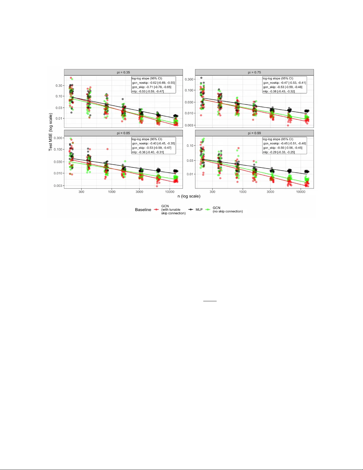
Semi-Sup ervised Learning on Graphs using Graph Neural Net w orks Jun tong Chen ∗ Claire Donnat † Olga Klopp ‡ Johannes Sc hmidt-Hieb er § ∗ Sc ho ol of Mathematical Sciences, Xiamen Universit y † Departmen t of Statistics, Universit y of Chicago ‡ ESSEC Business School § Departmen t of Applied Mathematics, Universit y of T w ente Abstract Graph neural net works (GNNs) w ork remarkably well in semi-supervised no de regression, y et a rigorous theory explaining when and why they succeed remains lacking. T o address this gap, w e study an aggregate-and-readout mo del that encompasses several common mes- sage passing arc hitectures: no de features are ﬁrst propagated o ver the graph then mapp ed to resp onses via a nonlinear function. F or least-squares estimation ov er GNNs with linear graph conv olutions and a deep ReLU readout, we pro ve a sharp non-asymptotic risk b ound that separates appro ximation, sto c hastic, and optimization errors. The b ound mak es explicit ho w p erformance scales with the fraction of lab eled no des and graph-induced dep endence. Appro ximation guaran tees are further derived for graph-smo othing follow ed by smo oth non- linear readouts, yielding con vergence rates that reco v er classical nonparametric behavior under full sup ervision while characterizing p erformance when lab els are scarce. Numerical exp erimen ts v alidate our theory , providing a systematic framework for understanding GNN p erformance and limitations. 1 In tro duction Graph Neural Net works (GNNs) ha v e b ecome the default to ol for semi-supervised prediction on graphs: giv en a graph G = ( V , E ) on n = |V | no des with features X i , w e observe a resp onse v ariable Y i on a subset of no des, and aim to predict the rest [ 35 , 49 , 52 , 66 ]. A cen tral assumption in this setting is that the graph sp eciﬁes how information propagates across no des, whic h, if eﬃcien tly lev eraged, can substan tially b oost prediction. GNNs ha ve ac hieved strong p erformance for no de-lev el prediction on in teraction graphs such as so cial or h yp erlink netw orks where they 1 predict outcomes like website traﬃc, future engagemen t, or satisfaction from partial lab els [ 4 , 12 , 34 ]. They are also increasingly used in spatially resolved omics, where no des are sp ots or cells connected b y spatial neigh b orho ods and the goal is to predict exp ensive assays (e.g., gene or protein measuremen ts) from observed mo dalities b y propagating lo cal con text through the graph [ 21 , 24 ]; we present real-data case studies in Section 4 . Semi-sup ervised learning on graphs has a rich and long history in the statistics literature. Classical graph semi-sup ervised learning is dominated by (i) Laplacian-based regularization [ 3 ] and (ii) lab el propagation [ 70 , 65 ]. While b oth of these approaches hav e b een extensiv ely studied and b eneﬁt from solid theoretical guarantees, they focus on spatial regularization, often ignoring no de features. By con trast, mo dern GNNs inject no de features in to propagation and deliv er strong empirical p erformance across domains. One of the k ey ingredien ts of their success lies in the use of message-passing lay ers that p erform a localized a veraging of features, eﬀectiv ely acting as a learnable low-pass ﬁlter on the graph signal [ 11 ]. The propagation rule enables the model to learn represen tations that are smooth across the graph and discriminative in their features. [ 28 ] empirically sho wed that graph con v olutional netw orks (GCNs), one of the earliest t yp es of GNNs, signiﬁcantly outperform manifold regularization and transductive SVMs, establishing GNNs as the dominant paradigm for graph semi-sup ervised learning. While a v ariety of GNN arc hitectures hav e b een prop osed (e.g. [ 60 , 69 ]), they largely share the same spirit: all inv olv e an initial aggregation of node information through a message-passing algorithm b efore its synthesis in to an output via a readout step (see App endix A for an extended discussion of related w orks). Despite their success in v arious practical applications, a rigorous statistical foundation for GNNs in the semi-sup ervised regime remains elusive. This theoretical gap is particularly strik- ing giv en the paradoxical empirical b eha vior of these mo dels: while GNNs can achiev e stable p erformance with limited lab els [ 41 ], they sim ultaneously exhibit high sensitivit y to structural p erturbations [ 15 , 71 ]. T o address this, w e study nonparametric semi-supervised no de regression under a comp ositional data-generating mechanism that lev erages message passing. W e fo cus on t wo k ey problems: (i) how graph-induced propagation aﬀects the eﬀective complexity of the pre- dictor, and (ii) ho w w ell the GNN class appro ximates the underlying regression function when it admits a propagation–nonlinearit y comp ositional form. The main contributions of this work are threefold: (i) A sharp oracle inequality for general estimators in the semi-sup ervised graph regression setting (Theorem 1 ) that decomp oses prediction error in to optimization error + approximation error + sto c hastic error. Crucially , our analysis explicitly characterizes ho w these errors dep end on the unmasked prop ortion and the graph’s top ology through a single parameter. (ii) Appro ximation theory for message passing: W e analyze the approximation capa- bilities of GNNs with linear graph conv olution lay ers follo w ed b y deep ReLU net works. W e show that this arc hitecture can approximate functions formed by the comp osition of 2 a graph-induced propagation step and a Hölder-smooth syn thesizing (readout) function (Lemma 4 ). (iii) Rates that expose lab el-scarcit y and graph eﬀects. Com bining (i) and (ii), w e deriv e explicit conv ergence rates for the least-squares GNN estimator (Theorem 2 ). With a properly c hosen arc hitecture (depth and width scaling with graph size), the estima- tor achiev es a conv ergence rate gov erned b y the smo othness of the underlying regression function and its intrinsic input dimension. Our analysis builds on the oracle-inequalit y and approximation-theoretic framework developed for sparse deep ReLU netw orks in classical nonparametric regression, most notably [ 46 ]. The semi-sup ervised graph setting, how ev er, introduces tw o core challenges that require nov el ana- lytical to ols. First, resp onses are observ ed only on a random subset of no des; we incorp orate this missingness mec hanism directly into the risk decomp osition to quantify the eﬀect of lim- ited sup ervision. Second, graph propagation induces non trivial statistical dep endencies b ecause predictions at each no de rely on ov erlapping neighborho o ds; we introduce a b ounded receptive ﬁeld assumption to model this graph-structured dep endency and, via graph coloring, develop concen tration arguments tailored to lo calized interactions. Com bined with new metric entrop y b ounds for the graph-con volutional comp onent and approximation guarantees for comp ositions of graph ﬁlters and Hölder-smo oth functions, this framew ork yields explicit non-asymptotic risk b ounds and con vergence rates for least-squares estimation ov er GNN classes. Notably , this gen- eral rate recov ers the optimal minimax rate for standard (non-graph) regression in the sp ecial case of full sup ervision and purely lo cal no de resp onses. This article is structured as follows. In Section 2 , we introduce the semi-sup ervised regression setting with graph-structured data. W e analyze GNN-based estimation in Section 3 , where, under a lo calit y condition, we establish an oracle inequality for any given estimator and explicitly c haracterize the con v ergence rate of the least squares estimator in terms of the prop ortion of lab eled no des and the graph’s receptiv e ﬁeld. Numerical experiments on b oth syn thetic and real-w orld datasets are presented in Section 4 . W e conclude in Section 5 and all the related pro ofs are provided in the App endix. Notation : W e set N 0 = { 0 , 1 , 2 , . . . } , N = { 1 , 2 , . . . } , R + = (0 , ∞ ) , and [ m ] = { 1 , . . . , m } . In this pap er, vectors and matrices are denoted by b old low ercase and upp ercase letters, respec- tiv ely . In sp eciﬁc contexts, we ma y use b old low ercase letters for ﬁxed matrices to distinguish them from their random counterparts. F or a d 1 × d 2 matrix M , deﬁne the entry-wise maxim um norm ∥ M ∥ ∞ = max i ∈ [ d 1 ] ,j ∈ [ d 2 ] | M i,j | , the row-sum norm ∥ M ∥ 1 , ∞ = max i ∈ [ d 1 ] X j ∈ [ d 2 ] | M i,j | , 3 and the F rob enius norm ∥ M ∥ F =  X i ∈ [ d 1 ] ,j ∈ [ d 2 ] M 2 i,j . W e denote the i -th ro w of M b y M i, · . F or p -dimensional ro w or column v ectors v = ( v 1 , . . . , v p ) , w e deﬁne | v | ∞ = max 1 ≤ i ≤ p | v i | and | v | 1 = P p i =1 | v i | . F or any a ∈ R , ⌊ a ⌋ denotes the largest in teger strictly less than a and ⌈ a ⌉ the smallest integer greater than or equal to a . W e use log 2 for the binary logarithm and log for the natural logarithm. F or a set C , we denote its cardinality b y |C | . F or tw o nonnegative sequences ( α n ) n and ( β n ) n , w e write α n ≲ β n if there exists a constan t c suc h that α n ≤ cβ n holds for all n , and w e write α n ≍ β n when α n ≲ β n ≲ α n . If the function v alue h ( x ) is a matrix, we denote the i -th row of h ( x ) by ( h ( x )) i or, if no am biguity arises, b y h i ( x ) . F or any tw o real-v alued functions f , g : X → R , their sup-norm distance is deﬁned as ∥ f − g ∥ L ∞ ( X ) = sup x ∈X | f ( x ) − g ( x ) | . F or any tw o v ector-v alued functions f = ( f 1 , . . . , f m ) ⊤ , g = ( g 1 , . . . , g m ) ⊤ where each comp onen t function satisﬁes f i , g i : X → R , the sup-norm distance b et ween f and g is deﬁned as ∥ f − g ∥ L ∞ ( X ) = max 1 ≤ i ≤ m sup x ∈X   f i ( x ) − g i ( x )   . When the domain X is clear from context, we simply write ∥ · ∥ ∞ . 2 Statistical setting Consider a graph G = ( V , E ) with v ertex set V and edge set E . Let n = |V | denote the num b er of v ertices. W e enco de the graph structure through its adjacency matrix A = ( A i,j ) ∈ { 0 , 1 } n × n , deﬁned by A i,j = ® 1 , if j ∈ N ( i ) , 0 , otherwise , where N ( i ) ⊆ V denotes the set of neighbors of no de i . W e deﬁne e A = A + I n as the adjacency matrix with self-loops, and let D and e D b e the corresponding diagonal degree matrices of A and e A , resp ectively . Each no de i ∈ { 1 , . . . , n } is assumed to hav e a feature v ector X i ∈ X , where X is a compact subset of R d . F or simplicit y , we assume X = [0 , 1] d throughout the pap er. W e assume that the feature v ectors X 1 , . . . , X n are indep enden t dra ws from distributions P X i on [0 , 1] d . The feature matrix X ∈ [0 , 1] n × d con tains X ⊤ i in its i -th row. In the semi-sup ervised framework, we observ e a random subset of no des Ω ⊆ V . F or each no de i ∈ Ω , b oth the feature vector X i and the resp onse Y i ∈ R are observed. F or no des in the complemen t Ω c = V \ Ω , only the features are av ailable. W e assume no des are included in Ω indep enden tly with probability π ∈ (0 , 1] , and denote b y ω i ∼ Bernoulli( π ) 4 the corresp onding Bernoulli indicator. The ob jectiv e is to predict the resp onse v alues for all no des in Ω c . This means that the (training) dataset is  X 1 , . . . , X n  ∪ { Y i } i ∈ Ω . (1) W e consider a no de-level regression problem on a graph, where resp onses asso ciated with indi- vidual no des dep end not only on their own features but also on the features of neighboring nodes through the graph structure. T o capture such structural dep endencies, w e adopt a comp ositional mo deling framework that separates feature propagation from lo cal prediction. F ormally , for eac h no de i ∈ { 1 , . . . , n } , the resp onse Y i is assumed to follow the statistical mo del Y i = φ ∗  ψ ∗ A ,i ( X )  + ε i , (2) for indep enden t ε i ∼ N (0 , 1) that are also indep enden t of X . The resulting (ov erall) regression function is given b y f ∗ = ( f ∗ 1 , . . . , f ∗ n ) ⊤ with f ∗ i = φ ∗ ◦ ψ ∗ A ,i , (3) and is assumed to admit a tw o-stage structure: the resp onse is obtained b y applying a shared nonlinear map φ ∗ : R d → R to the propagated features. The high-dimensional inner (regression) function ψ ∗ A : [0 , 1] n × d → [ − M , M ] n × d , maps to matrices with entries b ounded in absolute v alue by a chosen constan t M ≥ 1 ; the subscript A indicates the dep endence on the graph adjacency matrix. This function aggregates information across the graph to produce propagated no de features. Here, ψ ∗ A ,i : [0 , 1] n × d → [ − M , M ] 1 × d denotes the restriction of ψ ∗ A to its i -th row. In man y GNN architectures, feature propagation is implemented b y applying a linear graph ﬁlter to no de features. Common ﬁlters are p olynomials in a graph op erator, suc h as the Laplacian L = D − A , the adjacency ma- trix or normalized v ariants lik e e D − 1 / 2 e A e D − 1 / 2 and e D − 1 e A [ 10 , 28 , 32 ]. F urther examples are discussed in [ 28 , Section 6] and the survey [ 61 ]. Motiv ated b y these constructions, w e assume that the inner regression function ψ ∗ A is close to a matrix p olynomial with respect to a cho- sen graph propagation op erator S A . More precisely , let P k ( β , S A ) denote the set of functions ψ : [0 , 1] n × d → [ − M , M ] n × d of the form ψ ( x ) = k X j =1 θ j S j A x , (4) where S A is an n × n graph propagation op erator that leverages the connectivity enco ded in A , and the co eﬃcien ts θ j satisfy | θ j | ≤ β for some constant β > 0 . Typically , S A exhibits a lo w-dimensional structure, such as row-wise sparsity [ 22 , 64 ]. The j -th p o wer of S A c haracter- izes feature propagation o v er j hops, while the co eﬃcien ts θ j quan tify the inﬂuence of j -hop neigh b orho ods. T o accommo date settings where the propagation ma y only b e approximately p olynomial, due to nonlinearities or mo del mismatch, we introduce the ρ -neighborho o d F ρ ( β , k , S A ) = ß f : [0 , 1] n × d → [ − M ρ , M ρ ] n × d    inf g ∈P k ( β , S A ) sup x ∈X n ∥ f ( x ) − g ( x ) ∥ ∞ ≤ ρ ™ , (5) 5 with M ρ = M + ρ . W e then assume that the inner (regression) function satisﬁes ψ ∗ A ∈ F ρ ( β , k , S A ) . In the sp ecial case where S A is symmetric with eigendecomp osition S A = U ⊤ ΛU , an y f ∈ P k ( β , S A ) can b e expressed as f ( x ) = U ⊤ k X j =1 θ j Λ j ! U x . Consequen tly , a function g ( x ) = U ⊤ QU x lies within distance ρ (in sup-norm) of some f ∈ P k ( β , S A ) provided that the sp ectral ﬁlter Q satisﬁes ∥ Q − P ( Λ ) ∥ F ≤ ρ/ √ n , where P ( Λ ) = P k j =1 θ j Λ j . In particular, when ρ = 0 , the inner regression function simpliﬁes to the exact p olynomial form. Consequently , mo del ( 2 ) resembles a multi-index mo del, a class of functions extensively studied in recent theoretical deep learning literature [ 19 , 38 , 7 , 43 ]. Let v ec( X ) ∈ R nd denote the vectorized feature matrix X , and let V i ∈ R nd × d denote the linear map induced by S A . W e can then rewrite the mo del as Y i = φ ∗  V ⊤ i v ec( X )  + ε i . This form ulation reveals that eac h response dep ends on a low-dimensional pro jection of the global feature matrix, passed through a shared nonlinearity φ ∗ . Ho wev er, unlike the classical m ulti-index mo del where the pro jection is typically ﬁxed or unstructured, here the index maps { V i } n i =1 are node-sp eciﬁc and structurally constrained b y the graph top ology , reﬂecting the aggregation of lo cal neighborho o d information. 3 Estimation using GNNs In this section, we emplo y graph neural netw orks to approximate the target function and derive a generalization b ound for the resulting estimator. The architecture of the considered GNNs consists of tw o main comp onen ts: graph conv olutional la yers follow ed by deep feedforward neural net works. The precise architecture is sp eciﬁed in detail as follows. Graph con volutional netw orks (GCNs) provide a natural approach for approximating the target function ψ ∗ A that propagates no de feature information. A GCN typically takes the feature matrix x ∈ [0 , 1] n × d and a presp eciﬁed propagation matrix T as the input and pro duces a transformed version of the input feature matrix [ 28 ]. Sp eciﬁcally , let L represent the num b er of GCN lay ers. F or each ℓ ∈ { 0 , . . . , L − 1 } , the output of the lay ers can b e deﬁned recursively via H ( ℓ +1) T ( x ) = σ GCN  T H ( ℓ ) T ( x ) W ℓ +1  , (6) where H (0) T = x , σ GCN denotes the activ ation function, applied element-wise, and W ℓ +1 are d × d w eight matrices, whose entries are learnable parameters. Empirical studies demonstrate that 6 linear GCNs, that is, σ GCN = id , ac hiev e accuracy comparable to their nonlinear coun terparts in v arious downstream tasks [ 60 , 58 ]. Theoretically , [ 41 ] shows that nonlinearit y do es not enhance GCN expressivity . The linear setting has b een further explored under the name p oly-GNN in [ 57 ] and compared to standard GCNs in [ 39 , 40 ]. In particular, for the linear feature propagation deﬁned in ( 4 ), the iden tity function is a w ell-motiv ated choice for the activ ation; w e therefore set σ GCN = id . Dra wing inspiration from residual connections, w e aggregate the outputs of all conv olutional lay ers through a w eighted sum rather than using only the last la y er. This approac h of incorp orating connections from previous la yers preserves m ulti-scale represen tations from diﬀerent neighborho o d levels, th us mitigating the ov er-smoothing phenomenon [ 9 , 31 , 68 ]. A ccordingly , G ( L, T ) is deﬁned as the class of functions of the form P L ℓ =1 γ ℓ H ( ℓ ) T , that is G ( L, T ) = ( x 7→ L X ℓ =1 γ ℓ T ℓ x W 1 · · · W ℓ      W ℓ ∈ [ − 1 , 1] d × d and γ ℓ ∈ [ − 1 , 1] ) , (7) where the co eﬃcients γ ℓ are reweigh ting parameters. Deep feedforw ard neural netw orks are commonly applied after graph con v olutional lay ers to syn thesize the propagated feature vectors and pro duce ﬁnal no de-lev el outputs [ 67 , 61 , 62 ]. Here we follow the same paradigm and refer to this comp onen t as deep neural netw orks (DNNs). Let the width v ector p = ( p 0 , p 1 , . . . , p L +1 ) ∈ N L +2 satisfy p 0 = d and p L +1 = 1 , and let ReLU( u ) = max { 0 , u } denote the ReLU activ ation function. W e deﬁne F ( L, p ) as the class of deep ReLU neural netw orks of depth L ∈ N 0 and width vector p , comprising all functions f : R d → R of the form f ( x ) = Θ L ◦ ReLU ◦ Θ L − 1 ◦ · · · ◦ ReLU ◦ Θ 0 ( x ) , (8) where, for ℓ = 0 , . . . , L , Θ ℓ ( y ) = M ℓ y + b ℓ . Here, M ℓ is a p ℓ × p ℓ +1 w eight matrix, b ℓ is a bias v ector of size p ℓ +1 , and the ReLU activ ation function is applied comp onen t-wise to any given vector. Again, we assume that all en tries of the w eight matrices and bias vectors lie within [ − 1 , 1] . In practice, sparsity in neural netw orks is often encouraged through techniques such as regularization or sp ecialized arc hitectures [ 17 ]. A notable example is drop out, whic h promotes sparse activ ation patterns by randomly deactiv ating units during training, thereby ensuring that each neuron is activ e only for a small s ubset of the training data [ 51 ]. In line with the framew ork introduced b y [ 46 ], we explicitly enforce parameter sparsit y b y restricting the netw ork to utilize only a limited n umber of non-zero parameters. More precisely , let ∥ M ℓ ∥ 0 and | b ℓ | 0 denote the num b er of non-zero entries in the weigh t matrix M ℓ and bias v ector b ℓ , resp ectiv ely . F or any s ≥ 1 and F > 0 , we deﬁne the class of s -sparse DNNs, truncated to the range [ − F , F ] , as F ( L, p , s, F ) = ( ( f ∨ − F ) ∧ F : f ∈ F ( L, p ) , L X ℓ =0 ∥ M ℓ ∥ 0 + | b ℓ | 0 ≤ s ) . (9) 7 ( X 3 , Y 3 ) ( X 1 , Y 1 ) X 2 X 4 X 5 X 6 X 7 ( X ′ 1 , Y 1 ) GCN Comp onen t (F eature Propagation) b Y 1 X ′ 11 X ′ 1 d . . . DNN Comp onen t (Prediction) Input V ector X ′ 1 Figure 1: Graph feature propagation follow ed b y a nonlinear readout: a linear message-passing blo c k generates propagated features, whic h are then mapped to no de-lev el predictions via a ReLU DNN. In conclusion, the considered graph neural netw orks class is given by F ( T , L 1 , L 2 , p , s, F ) = n f : f i ( x ) = h  g i ( x )  , h ∈ F ( L 2 , p , s, F ) , g ∈ G ( L 1 , T ) o , (10) where L 1 , L 2 ∈ N 0 are the resp ective depths of the con volutional and feedforward lay ers, and T is a pre-sp eciﬁed conv olutional op erator. Figure 1 provides a schematic explanation of the constituen t blo c ks. An y estimator of the regression function is based on the training data { X 1 , . . . , X n } ∪ { Y i } i ∈ Ω with Ω the random set of unmask ed response v ariables. The statistical p erformance of an estimator e f = ( e f 1 , . . . , e f n ) ⊤ : [0 , 1] n × d → R n is measured by the prediction error R Ä e f , f ∗ ä = E ñ 1 n n X i =1 Ä e f i ( X ′ ) − φ ∗  ψ ∗ A ,i ( X ′ )  ä 2 ô , (11) where X ′ is an indep enden t copy of X and the exp ectation is taken ov er all the randomness in the mo del, that is, the randomness induced by Ω ∪ { ( X i , X ′ i , ε i ) } n i =1 . Among v arious estimators, we are primarily interested in analyzing the p erformance of the least-squares estimator ov er the class F ( T , L 1 , L 2 , p , s, F ) constructed from the unmask ed no des in Ω ⊆ { 1 , . . . , n } , that is, b f ∈ argmin f ∈F ( T ,L 1 ,L 2 , p ,s,F ) 1 n X i ∈ Ω  Y i − f i ( X )  2 . (12) By the deﬁnition of F ( T , L 1 , L 2 , p , s, F ) , this estimator admits a decomp osition satisfying for all i ∈ Ω , b f i ( X ) = b φ ◦ b ψ i ( X ) , where b φ ∈ F ( L 2 , p , s, F ) and b ψ ∈ G ( L 1 , T ) . 8 3.1 Oracle-t yp e inequality W e b egin by introducing the prerequisites. Let ε = ( ε 1 , . . . , ε n ) ⊤ and ω = ( ω 1 , . . . , ω n ) ⊤ . F or an y estimator e f returning a netw ork in F with output e f i at the i -th no de, the optimization error is deﬁned as ∆ F n Ä e f , f ∗ ä = E ε , ω , X " 1 n X i ∈ Ω  Y i − e f i ( X )  2 − inf f ∈F 1 n X i ∈ Ω  Y i − f i ( X )  2 # . (13) It measures the exp ected diﬀerence b et ween the training loss of e f and the training loss of the global minimum ov er all net w ork ﬁts in the class F , where the data { ( X i , Y i ) } are generated according to the true regression function f ∗ in ( 3 ). The optimization error is nonnegative and v anishes if e f is an empirical risk minimizer ov er F . The complexity of the vector-v alued function class F is measured by its metric entrop y . Recall that for any tw o functions f , g : X n → R n , with f = ( f 1 , . . . , f n ) ⊤ and g = ( g 1 , . . . , g n ) ⊤ , their sup-norm distance is giv en b y ∥ f − g ∥ ∞ = max 1 ≤ i ≤ n ∥ f i − g i ∥ ∞ . F or any δ > 0 , we sa y a class of functions F ′ is a δ -cov er of F with resp ect to the sup-norm, if for any f ∈ F , there exists a function g ∈ F ′ suc h that ∥ f − g ∥ ∞ ≤ δ . W e denote the smallest δ -co ver of F b y F δ . The δ -cov ering num ber N ( δ , F , ∥ · ∥ ∞ ) is the cardinality of F δ . If no ﬁnite δ -co ver exists, the co vering num b er is deﬁned to b e inﬁnite. The metric entrop y (or simply entrop y) of F at scale δ > 0 is log N ( δ, F , ∥ · ∥ ∞ ) . F or brevity , we simplify this notation in some con texts to log N δ . A k ey insight from statistical learning theory is that the sto c hastic error dep ends critically on this measure of mo del complexity [ 55 , 2 , 46 ]. A k ey technical diﬀerence with standard nonparametric regression is that, even if the no de features { X i } n i =1 are sampled indep enden tly and the noises { ε i } n i =1 are indep endent, the empir- ical loss is not a sum of indep enden t terms once prediction uses graph propagation. Indeed, for a general graph-based predictor f ∈ F , each no dal output f i ( X ) may dep end on the features of man y no des through message passing, so the squared error contributions from each no de i , s ( f ) i ( X ) =  f i ( X ) − f ∗ i ( X )  2 can b e statistically coupled through shared co ordinates of X . T o quantify this dep endence in the analysis, we formalize a b ounded-inﬂuence prop erty: each no dal loss s ( f ) i ( X ) dep ends on features from only a limited n umber of no des, while the features from any given no de aﬀect at most a b ounded num b er of loss terms. The following assumption captures this via a single parameter m , which will app ear as a multiplicativ e factor in the oracle inequality and can b e in terpreted as an upp er b ound on the eﬀective receptive-ﬁeld size under graph propagation. W e now state this lo calit y condition formally as an assumption on the true regression function f ∗ and the base class F . Assumption 1. L et m b e a p ositive inte ger. F or any f = ( f 1 , . . . , f n ) ⊤ ∈ F ⊂ { g : R n × d → R n } , f ∗ = ( f ∗ 1 , . . . , f ∗ n ) ⊤ , and any ar gument x ∈ R n × d , assume that 9 (i) e ach function x 7→ s ( f ) i ( x ) =  f i ( x ) − f ∗ i ( x )  2 with i ∈ [ n ] dep ends on at most m c o or dinates of x = ( x 1 , . . . , x n ) ⊤ ; (ii) e ach c o or dinate x j inﬂuenc es at most m functions s ( f ) i . This assumption naturally arises from common graph propagation mec hanisms and GNN arc hitectures. F or instance, consider a k -step p olynomial ﬁlter f ( x ) = P k j =1 θ j S j x , where the propagation matrix S is symmetric and corresp onds to an undirected graph of maxim um degree ∆ (with self-lo ops). In this case, each output f i ( x ) dep ends only on features within k hops of no de i , and one may c ho ose m = ∆ k . Similarly , for a depth- L 1 linear GCN with propagation matrix T (unit diagonal) and with at most m T non-zero entries p er row and p er column, each no dal output dep ends on at most m L 1 T input feature vectors; hence we may tak e m = m L 1 T . Building up on the existing no de graph, Assumption 1 allows us to deﬁne a new dep endency graph for { s ( f ) i } n i =1 . An edge b et ween no des i and j in this dep endency graph exists when s ( f ) i and s ( f ) j share a common input co ordinate. Under Assumption 1 , this graph has maxim um degree at most m ( m − 1) . A direct implication of this b ounded degree is the existence of a (disjoin t) partition P 1 ∪ · · · ∪ P r = { 1 , . . . , n } with r ≤ m ( m − 1) + 1 . Here, eac h part P ℓ comprises indices such that for any distinct i, j ∈ P ℓ , the losses s ( f ) i ( X ) and s ( f ) j ( X ) share no co v ariate v ector. This key insight makes it p ossible to deriv e tigh t concen tration b ounds for functions exhibiting this type of sparse lo cal dep endence. The following theorem states an oracle-type inequalit y that holds for any estimator e f con- structed from a general mo del class F . Theorem 1. Assume Assumption 1 holds with m ≥ 1 . F or 0 < δ ≤ 1 , let F δ b e a δ -cov er of F whose entrop y satisﬁes log N δ ≥ 1 . Supp ose that there exists a constan t F ≥ 1 such that ∥ f i ∥ ∞ ≤ F for all i ∈ [ n ] and all f ∈ F ∪ F δ ∪ { f ∗ } . Then, for any ε ∈ (0 , 1] , (1 − ε ) 2 ∆ F n ( e f , f ∗ ) − E 1 ( ε, n, δ ) ≤ R ( e f , f ∗ ) ≤ 2(1 + ε ) 2 Ç inf f ∈F E ñ 1 n n X i =1  f i ( X ) − f ∗ i ( X )  2 ô + ∆ F n ( e f , f ∗ ) π + E 2 ( ε, n, π , δ ) å , where E 1 ( ε, n, δ ) = C 1 Å m 2 F 2 log N δ εn + δ F ã , E 2 ( ε, n, π , δ ) = C 2 ï (1 + ε ) m 2 F 2 log N δ εnπ + F δ √ π + F 2 N δ ò , with C 1 , C 2 > 0 univ ersal constants. The pro of of Theorem 1 is p ostponed to Section D . The result indicates that the upp er b ound for the prediction error of an arbitrary estimator e f based on mo del F can b e decomp osed in to 10 three main terms: the appro ximation error b et ween F and the target f ∗ , the sto c hastic error E 2 ( ε, n, π , δ ) go verned b y the complexit y of F , and the optimization error ∆ F n ( e f , f ∗ ) , whic h quan tiﬁes the training error discrepancy betw een the chosen estimator and the empirical risk minimizer. When π = 1 (full sup ervision) and pro vided the co vering num b er N δ is not to o small, our result recov ers the same dep endence on n as in standard regression [ 46 ] (Theorem 2). The b ounds diﬀer by a m ultiplicative factor of m 2 , which accounts for the graph-induced dep endency . The distinct roles of m and π in Theorem 1 shed ligh t on the seemingly con tradictory phenomena observed in practice. On one hand, the upp er b ound is scaled by the expected prop ortion of observ ed sample pairs π ; when π remains constant, even if small, the p rediction error increases only by a constant multiplicativ e factor. This explains why GNNs can achiev e satisfactory generalization with limited supervision [ 32 , 28 ]. On the other hand, structural p erturbations suc h as edge rewiring or dropping can fundamentally alter the graph geometry , resulting in performance instabilit y [ 15 , 71 ]. In our bound, this sensitivit y is quan tiﬁed b y the receptive ﬁeld size m , which dep ends in tricately on the netw ork’s expansion prop erties. F or instance, in a ring lattice, m grows only linearly with the n umber of propagation steps. Ho wev er, adding a few “shortcut” edges triggers a phase transition to a small-w orld regime, where the neigh b orho od size m may shift from linear to exp onen tial expansion [ 59 ]. Such structural shifts signiﬁcan tly relax the generalization b ounds, thereby accounting for the high sensitivit y of GNNs to top ological p erturbations that bridge distan t clusters. In what follo ws, w e pro vide a more precise analysis fo cusing on the prop osed GNN class F ( T , L 1 , L 2 , p , s, F ) . The result b elo w establishes an upp er bound for the metric en tropy of F ( T , L 1 , L 2 , p , s, ∞ ) . Because the inequality   ( f ∨ − F ) ∧ F − ( g ∨ − F ) ∧ F   ∞ ≤ ∥ f − g ∥ ∞ holds, the same entrop y b ound immediately extends to the b ounded class F ( T , L 1 , L 2 , p , s, F ) . Recall that for a matrix M = ( M i,j ) , the row-sum norm is ∥ M ∥ 1 , ∞ = max i P j | M i,j | . Prop osition 1. Let L 1 ≥ 1 . F or any 0 < δ ≤ 1 , log N  δ, F ( T , L 1 , L 2 , p , s, ∞ ) , ∥ · ∥ ∞  ≤  d 2 L 1 + L 1 + s + 1  log L ( L 1 , L 2 ) δ L 2 +1 Y k =0 ( p k + 1) 2 ! , where L ( L 1 , L 2 ) = 2 L 1 ( L 1 + L 2 + 2)( ∥ T ∥ 1 , ∞ ∨ 1) L 1 d L 1 . The pro of of Prop osition 1 is deferred to Section E . Observ e that the considered GNNs hav e a total of ( d 2 + 1) L 1 + s trainable parameters. In practice, GCNs emplo y few lay ers, so L 1 is typically indep enden t of n , and the feature dimension d is also commonly assumed to b e ﬁnite [ 48 , 45 ]. When the widths p k of the deep ReLU netw orks are b ounded by order n γ and n is suﬃciently large, the logarithmic term simpliﬁes to ≲ L 2 log[( n γ ∨ L 2 ) /δ ] for any δ ≤ 1 . Consequen tly , up to a constant factor dep ending on ∥ T ∥ 1 , ∞ , d , and L 1 , the metric entrop y of 11 F ( T , L 1 , L 2 , p , s, F ) at scale δ ≤ 1 can b e b ounded b y ≲ sL 2 log[( n γ ∨ L 2 ) /δ ] . Therefore, the depth and sparsit y of the DNN comp onen t pla y an essen tial role in determining the en tropy . Based on Theorem 1 and Prop osition 1 , we obtain the following result. Corollary 2. Supp ose Assumption 1 holds with m ≥ 1 , and the true regression function f ∗ satisﬁes ∥ f ∗ i ∥ ∞ ≤ F for all i ∈ [ n ] and some F ≥ 1 . Let e f be an y estimator in the class F = F ( T , L 1 , L 2 , p , s, F ) , where s ≥ 2 and L 1 , L 2 ≥ 1 . Assume N  1 /n, F , ∥·∥ ∞  ≳ n. Deﬁne κ n = ( d 2 L 1 + s )  log  nL 1 ( L 1 + L 2 )  + ( L 1 + 1) log  ∥ T ∥ 1 , ∞ ∨ d  + L 2 log s  . Then, for any ε ∈ (0 , 1] , there exists C ε > 0 dep ending only on ε such that (1 − ε ) 2 ∆ F n ( e f , f ∗ ) − C ε m 2 F 2 κ n n ≤ R ( e f , f ∗ ) ≤ 2(1 + ε ) 2 ñ inf f ∈F ( T ,L 1 ,L 2 , p ,s,F ) ∥ f − f ∗ ∥ 2 ∞ + ∆ F n ( e f , f ∗ ) π ô + C ε m 2 F 2 π κ n n . The pro of of Corollary 2 is p ostp oned to Section D . Theorem 1 and Corollary 2 provide not only an upper b ound but also a low er b ound on the prediction error in terms of the optimization error ∆ F n ( e f , f ∗ ) . In particular, Corollary 2 implies that for any ε ∈ (0 , 1] , R ( e f , f ∗ ) ≥ (1 − ε ) 2 ∆ F n ( e f , f ∗ ) − C ε m 2 F 2 κ n n , for a p ositiv e constant C ε . Consequen tly , the optimization error acts as a ﬂo or for the achiev- able prediction accuracy: unless the training algorithm returns an approximate empirical risk minimizer with ∆ F n ( e f , f ∗ ) ≲ m 2 F 2 κ n /n , the prediction risk cannot achiev e the statistical rate implied b y the mo del complexit y . This highlights an explicit computational–statistical trade-oﬀ in our setting: to b eneﬁt from the statistical guarantees, the optimization error must b e driv en b elo w the intrinsic “statistical resolution” of the function class. When e f = b f is the empirical minimizer deﬁned as in ( 12 ), the optimization error ∆ F n ( b f , f ∗ ) is zero and the error upp er b ound reveals a bias-v ariance trade-oﬀ b et ween the approximation error of f ∗ based on mo del F ( T , L 1 , L 2 , p , s, F ) and the v ariance terms dep ending on the complexity of F ( T , L 1 , L 2 , p , s, F ) . F or b oth GCN and DNN components, stacking to o many lay ers worsens the upp er b ound, as this is reﬂected in the term κ n . 3.2 Appro ximation with GNNs This section analyzes the appro ximation capabilit y of the class F ( T , L 1 , L 2 , p , s, F ) deﬁned in ( 10 ), whic h ultimately provides the appro ximation error inf f ∈F ( T ,L 1 ,L 2 , p ,s,F ) ∥ f − f ∗ ∥ ∞ in Corollary 2 . W e ﬁrst consider the approximation of the target class F 0 ( β , k , T ) by the GCN class G ( L 1 , T ) . 12 Lemma 3. Let F 0 ( β , k , T ) b e the function class deﬁned in ( 5 ). If L 1 ≥ k , and β ≤ 1 , then F 0 ( β , k , T ) ⊆ G ( L 1 , T ) . The pro of of Lemma 3 is deferred to Section F . The ab o ve result demonstrates that, when the propagation op erators coincide, GCNs with suﬃcient depth and parameters constrained to [ − 1 , 1] contain the function class F 0 ( β , k , T ) with normalized co eﬃcien ts. Additionally , for any function f ∈ F ρ ( β , k , T ) with ρ > 0 , Lemma 3 implies that there exists g ∈ G ( L 1 , T ) satisfying ∥ f − g ∥ ∞ ≤ ρ . In the case where β > 1 , any f ∈ F 0 ( β , k , T ) can be expressed as f = β h , where h ∈ F 0 (1 , k , T ) . Th us, the original approximation problem reduces to approximating the normalized function class F 0 (1 , k , T ) , while the scaling factor β will b e handled separately b y the DNN comp onent. A k ey feature of the GNN class deﬁned in ( 10 ) is that it produces predictions through succes- siv e nonlinear transformations applied to the propagated features: the DNN “readout” is itself a comp osition of simple maps (aﬃne transformations and p oin twise nonlinearities). Motiv ated b y this arc hitectural structure, w e mo del φ ∗ as a ﬁnite comp osition of smo oth, lo w-dimensional building blo c ks, allowing complex dep endencies in d v ariables to b e assembled hierarchically from simpler interactions. Bey ond matc hing the net work structure, this assumption is also statisti- cally meaningful: if each intermediate comp onen t dep ends only on a small num b er of v ariables, then appro ximation and estimation rates are gov erned by the corresp onding in trinsic dimensions rather than the am bient dimension d . This helps mitigate the curse of dimensionality , as shown e.g. in [ 46 , 26 , 1 ]. Concretely , we assume that φ ∗ admits the representation φ ∗ = g ∗ q ◦ g ∗ q − 1 ◦ · · · ◦ g ∗ 0 , where each g ∗ i = ( g ∗ i, 1 , . . . , g ∗ i,d i +1 ) ⊤ maps [ a i , b i ] d i to [ a i +1 , b i +1 ] d i +1 . F urthermore, for every j ∈ { 1 , . . . , d i +1 } , we assume that g ∗ i,j is α i -Hölder smo oth and dep ends on at most t i v ariables. W e no w formalize this notion b y recalling Hölder balls and then deﬁning the resulting compositional function class. F or any α > 0 , we sa y a function f is of α -Hölder smo othness if all its partial deriv atives up to order ⌊ α ⌋ exist and are b ounded, and the partial deriv atives of order ⌊ α ⌋ are ( α − ⌊ α ⌋ ) -Hölder con tinuous. Given t ∈ N and α > 0 , deﬁne the α -Hölder ball with radius K ≥ 0 , denoted by H α t ( D , K ) , as the collection of functions f : D ⊂ R t → R suc h that X β =( β 1 ,...,β t ) ∈ N t 0 P t j =1 β j <α ∥ ∂ β f ∥ ∞ + X β ∈ N t 0 P t j =1 β j = ⌊ α ⌋ sup x , y ∈D x  = y   ∂ β f ( x ) − ∂ β f ( y )   | x − y | α −⌊ α ⌋ ∞ ≤ K , where for any β = ( β 1 , . . . , β t ) ∈ N t 0 , ∂ β = ∂ β 1 · · · ∂ β t . Within the framework, we assume that eac h constituent function g ∗ i,j ∈ H α i t i ([ a i , b i ] t i , K ) . 13 Consequen tly , the underlying comp ositional function class is given b y G ( q , d , t , α , K ) = ¶ g q ◦ · · · ◦ g 0 : g i = ( g i,j ) j : [ a i , b i ] d i → [ a i +1 , b i +1 ] d i +1 , g i,j ∈ H α i t i ([ a i , b i ] t i , K ) , for some | a i | , | b i | ≤ K © , (14) where q ∈ N 0 , d = ( d 0 , . . . , d q +1 ) ∈ N q +2 with d 0 = 1 and d q +1 = 1 , t = ( t 0 , . . . , t q ) ∈ N q +1 , α = ( α 0 , . . . , α q ) ∈ R q +1 + , and K ≥ 0 . The i -th en try t i of the v ector t indicates the eﬀectiv e input dimension for every g i,j , with j = 1 , . . . , d i +1 . F or an y function f = g q ◦ · · · ◦ g 0 ∈ G ( q , d , t , α , K ) , where each comp onen t g i p ossesses certain smo othness prop erties, the ov erall comp osition f exhibits a sp eciﬁc lev el of smo othness determined b y its constituents. The classical d -v ariate Hölder class corresp onds to the sp ecial case where q = 0 and t 0 = d . In contrast, for the case q = 1 with α 0 , α 1 ≤ 1 and d 0 = d 1 = t 0 = t 1 = 1 , the comp osite function f = g 1 ◦ g 0 ac hieves a smo othness of order α 0 α 1 , as established in [ 44 , 26 , 1 ]. F or general compositions, the eﬀectiv e smo othness parameters are deﬁned for i = 0 , . . . , q − 1 by α ∗ i = α i q Y ℓ = i +1 ( α ℓ ∧ 1) , (15) with α ∗ q = α q . These parameters inﬂuence the con vergence rate of the netw ork estimator. Previous studies hav e established that deep ReLU netw orks are capable of eﬀectiv ely ap- pro ximating comp ositional smooth function classes [ 46 , 8 ]. Combined with Lemma 3 , this leads to the follo wing approximation error bound, proving that the target regression function class F ρ ( β , k , S A ) can b e well approximated b y F ( S A , L 1 , L 2 , p , s, F ) with appropriate architecture. Lemma 4. Let φ ∗ ∈ G ( q , d , t , α , K ) with K ≥ 1 b e deﬁned in ( 14 ), and let ψ ∗ A ∈ F ρ ( β , k , S A ) with ρ < 1 b e deﬁned in ( 5 ). Set Q 0 = 1 , Q i = (2 K ) α i for i ∈ [ q − 1] , and Q q = K (2 K ) α q . F or any N i ∈ N such that N i ≥ ( α i + 1) t i ∨ ( Q i + 1) e t i , there exists f ∈ F ( S A , L 1 , L 2 , p , s, F ) satisfying L 1 ≥ k , L 2 ≤ C 3 log 2 n, N = max i =0 ,...,q N i , s ≤ C 4 N log 2 n p = Å d, 3 ° β M § d, C 5 N , . . . , C 5 N , 1 ã , and F ≥ K, suc h that for every f ∗ j = φ ∗ ◦ ψ ∗ A ,j , j = 1 , . . . , n , ∥ f j − f ∗ j ∥ ∞ ≤ C 6 " q X i =0 Å N − α i t i i + N i n − α i + t i 2 α ∗ i + t i ã Q q ℓ = i +1 ( α ℓ ∧ 1) + ρ Q q i =0 ( α i ∧ 1) # , where C 3 , C 4 , C 5 , C 6 are numerical constants that do not dep end on n . The pro of is p ostponed to Section F . Lemma 4 decomp oses the appro ximation error into t wo terms asso ciated with approximating F ρ ( β , k , S A ) and G ( q, d , t , α , K ) . The eﬀective smo othness 14 α ∗ i quan tify the appro ximation rate. In particular, when N i ≍ n t i / (2 α ∗ i + t i ) holds for all i , the ﬁrst term in the brack et b ecomes q X i =0 Å N − α i t i i + N i n − α i + t i 2 α ∗ i + t i ã Q q ℓ = i +1 ( α ℓ ∧ 1) ≲ q max i =0 ,...,q n − α ∗ i 2 α ∗ i + t i . This scenario arises when we later incorporate the mo del complexit y from Prop osition 1 to determine an appropriate netw ork arc hitecture for estimation. The preceding analysis characterizes the appro ximation error asso ciated with using the true propagation op erator S A . F or practical situations where the implemen ted op erator T deviates from S A , the next result shows that this deviation introduces an additional error term b ey ond ρ . Lemma 5. Let T and S A b e n × n matrices with resp ectiv e row sparsity at most d T and d S A . If ∥ T − S A ∥ F ≤ τ , then for an y p ositiv e integer L 1 , any ro w index j ∈ { 1 , . . . , n } , and any x ∈ [0 , 1] n × d , we hav e       L 1 X i =1 θ i ( T i − S i A ) x ! j, ·       ∞ ≤ τ p d T + d S A " L 1 X i =1 i | θ i |  ∥ T ∥ 1 , ∞ ∨ ∥ S A ∥ 1 , ∞  i − 1 # . The pro of is giv en in Section F . Lemma 5 shows that the additional approximation error induced by using an implemen ted propagation op erator T instead of the target op erator S A is con trolled b y three factors: (i) their Euclidean distance τ = ∥ T − S A ∥ F , (ii) the lo cal sparsity lev els d T , d S (n umber of nonzeros p er row), and (iii) an ampliﬁcation term P L 1 i =1 i | θ i | ( ∥ T ∥ 1 , ∞ ∨ ∥ S A ∥ 1 , ∞ ) i − 1 arising from rep eated propagation. In particular, if L 1 and {| θ i |} L 1 i =1 are treated as constan ts, the mismatch contribution scales as ≲ τ p d T + d S A . F or sparse “real-life” netw orks, it is natural to assume that the n umber of connections p er no de grows slo wly with n ; a common regime, as shown in [ 5 , 63 ], is d T , d S A ≲ log n. Under this logarithmic-degree scaling, Lemma 5 yields a mismatc h term of order τ √ log n pro- vided ∥ T ∥ 1 , ∞ ∨ ∥ S A ∥ 1 , ∞ remains O (1) , a condition satisﬁed by commonly used normalized prop- agation op erators suc h as row sto c hastic matrices. If instead T is an unnormalized adjacency- t yp e op erator with O (1) weigh ts, then ∥ T ∥ 1 , ∞ t ypically scales like the maxim um degree and hence also ≲ log n in this regime, yielding an at-most p olylogarithmic dep endence on n through P L 1 i =1 | θ i | i (log n ) i − 1 (and therefore ≲ τ (log n ) L 1 − 1 / 2 when L 1 is ﬁxed). 3.3 Con v ergence rate of the least-squares estimator Throughout th is section, we assume that the propagation function ψ ∗ A ∈ F 0 ( β , k , S A ) and the outer function φ ∗ ∈ G ( q , d , t , α , K ) . The aim is to examine the rate of conv ergence of the least-squares estimator b f deﬁned in ( 12 ) ov er the class F ( S A , L 1 , L 2 , p , s, F ) . 15 By deﬁnition ( 13 ), the optimization error ∆ F ( S A ,L 1 ,L 2 , p ,s,F ) n ( b f , f ∗ ) v anishes if b f is the em- pirical risk minimizer. Therefore, Corollary 2 sho ws that the prediction error of b f admits a bias-v ariance decomp osition consisting of a bias term plus a v ariance term that dep ends on the net work class. Prop osition 1 and Lemma 4 demonstrate that using netw ork mo dels with more parameters increases the v ariance while t ypically reducing the bias. In the next result, we sho w that when the net w ork architecture is well-c hosen, the least-squares estimator b f conv erges to the true regression function. Theorem 2. Supp ose Assumption 1 holds for some m ≥ 1 and that the unknown regression function f ∗ has i -th component of the form f ∗ i = φ ∗ ◦ ψ ∗ A ,i , where φ ∗ ∈ G ( q, d , t , α , K ) with K ≥ 1 and ψ ∗ A ∈ F 0 ( β , k , S A ) . Set N i = ⌈ n t i / ( t i +2 α ∗ i ) ⌉ , N = max i =0 ,...,q N i , and let b f b e the least-squares estimator ov er the netw ork class F ( S A , L 1 , L 2 , p n , s n , F ) , where the netw ork arc hitecture satisﬁes (i) L 1 ≥ k ; (ii) 1 ≤ L 2 ≤ C 7 log 2 n ; (iii) p n = Ä d, 3 ⌈ β M ⌉ d, C 8 N , . . . , C 8 N , 1 ä ; (iv) 2 ≤ s n ≤ C 9 N log 2 n ; (v) F ≥ K . Then, for all suﬃciently large n , R ( b f , f ∗ ) ≤ C 10 m 2 log 3 n π max i =0 ,...,q n − 2 α ∗ i 2 α ∗ i + t i . Here, C 7 , C 8 , C 9 , C 10 are numerical constants indep endent of n . The pro of follo ws from a consequence of Lemma 4 and Corollary 2 , and is deferred to Section D . Theorem 2 pro vides an explicit non-asymptotic conv ergence rate for the least-squares estimator o v er the GNN class F ( S A , L 1 , L 2 , p n , s n , F ) under the compositional mo del f ∗ i = φ ∗ ◦ ψ ∗ A ,i . The b ound exhibits the following salient features. The con v ergence rate is go v erned by the in trinsic regularity of φ ∗ , sp eciﬁcally by its eﬀective smo othness parameters α ∗ i deﬁned in ( 15 ) and the asso ciated intrinsic dimensions t i . Ultimately , the ov erall rate is determined b y the b ottlenec k max i =0 ,...,q n − 2 α ∗ i / (2 α ∗ i + t i ) . In particular, in the classical Hölder case ( q = 0 , t 0 = d ), Theorem 2 reco vers the minimax-optimal rate n − 2 α/ (2 α + d ) in terms of the sample size n , up to logarithmic factors. F or target functions φ ∗ with a gen uinely comp ositional structure, ho w ever, the con v ergence rate dep ends only on the smaller intrinsic dimensions t i , thereby mitigating the curse of dimensionality . While matching the minimax rate with resp ect to the sample size n , as noted b elow The- orem 1 , the factor m 2 /π c haracterizes a key departure from standard regression, explicitly quan tifying the interaction b et w een graph-induced dep endence and semi-sup ervised learning. F or graphs of bounded degree with ﬁxed propagation depth, m is essen tially constant (up to 16 p olylog factors). When m grows rapidly with n (for instance, due to large depth L 1 or the presence of high-degree h ubs), the com bined term m 2 /π may dominate. This rev eals an explicit bias-v ariance trade-oﬀ in message passing: while increasing L 1 (or employing less lo calized prop- agation) reduces approximation bias for ψ ∗ A , it simultaneously increases the dep endence p enalt y through m . Th us, L 1 should b e k ept near the target ﬁlter order k , and normalized propagation op erators (with b ounded ∥ S A ∥ 1 , ∞ ) are recommended to control constants. 4 Numerical exp erimen ts In this section, w e empirically v alidate our theoretical ﬁndings through syn thetic and real w orld exp erimen ts. Speciﬁcally , we seek to (i) conﬁrm the con vergence rate of the prediction error as a function of the sample size n (as provided by Theorem 2 ), and (ii) ev aluate how the graph top ology , as captured by the av erage and maxim um degree ∆ , aﬀects the deca y rate of the MSE. T o this end, we compare four neural netw ork architectures: • MLP (no propagation). Set Z = X and predict b Y = b f ( Z ) with a ReLU MLP b f ∈ DNN L D , where L D denotes the depth of the neural netw ork. • GCN (no skip connections). Propagate features with L G ∈ { 1 , 2 , 3 } linear GCN la y ers b g ∈ GCN L G to obtain Z = b g ( X ) , then predict with an MLP head b Y = b f ( Z ) , ˆ f ∈ DNN L D . • GCN (skip connections). Compute la y erwise representations H ( ℓ ) S A ( X ) and form a con vex com bination Z = P L ℓ =1 w ℓ H ( ℓ ) S A ( X ) with w ℓ = exp( α ℓ ) / P L k =1 exp( α k ) , then predict b Y = b f ( Z ) with b f ∈ DNN L D . • MaGNet-inspired m ulti-scale model . W e adapt MaGNet to no de regression by ag- gregating multi-hop linear con volutions H ( ℓ ) S ( X ) = S ℓ XW with S = D − 1 / 2 AD − 1 / 2 (no self-lo ops), forming Z = P L ℓ =1 w ℓ H ( ℓ ) S ( X ) , and applying an MLP head no de-wise. The fusion weigh ts w ℓ are either learned end-to-end or set via the critic mo de of [ 68 ]. 4.1 Ev aluating con v ergence rate T o ev aluate the results established in Theorem 2 , w e consider a cycle (ring) graph with n no des and a b ounded degree of ∆ = 3 (including self-lo ops). W e generate node features as X i i.i.d. ∼ Unif [0 , 1] and construct propagated features as Z = k X j =1 θ j S j A X , 17 Figure 2: MSE (ov er 20 trials) as a function of training samples n , with the unmasked prop ortion held constant at π ∈ { 0 . 35 , 0 . 75 , 0 . 85 , 0 . 95 } . Estimators are distinguished by color: GCN with skip connections, GCN without skip connections, and the MLP baseline. where S A is taken as a neighborho o d a verage and the co eﬃcien ts θ j are b ounded. The resp onses are generated as Y i = φ ∗ ( Z i, · ) + ε i with ε i i.i.d. ∼ N (0 , 1) . W e set φ ∗ ( z ) = BM  Sigmoid  z scale  , where BM denotes a sample path of a Brownian motion, obtained by discretizing the interv al [0 , 1] in to 2 12 equal-length subin terv als. This ensures that φ ∗ has Hölder regularity α ≈ 1 / 2 [ 30 ]. Node resp onses Y i are observed on a random subset (inclusion probabilit y π ). Models are trained and ev aluated on an indep enden t cop y of the features X ′ . Results are compared across metho ds and for diﬀeren t v alues of π in Figure 2 . Recall that Theorem 2 p oin ts to a learning rate of order n − 2 α/ (2 α + t ) . F or the considered sim ulation setup, t = 1 and α is close to 1 / 2 . Theorem 2 th us p ostulates a conv ergence rate of approximately n − 1 / 2 in this setting. As shown in Figure 2 , for large training sets (high π ), the ﬁtted slop e is appro ximately − 1 / 2 , in go o d agreement with the theoretical prediction. W e also note, how ever, that for v ery lo w π , the slop e deviates from its exp ected v alue; This is particularly salient in Figure 3 , where w e 18 Figure 3: Left: Fitted slop es of log (MSE) vs. log( n ) as a function of connection probability π . Righ t : log(MSE) as a function of the eﬀectiv e sample size n eﬀ = n × π for the GCN with skip connections, as prop osed in Equation ( 7 ). plot the ﬁtted slop e as a function of the prop ortion of training data π , and observe signiﬁcan tly lo wer slop es for extremely small v alues of π (for instance, around − 0 . 95 for π = 0 . 01 ). This eﬀect could b e explained b y an increase in the relative contribution of the optimization error in lo w-data regimes (consistent with Corollary 2 , which p osits that optimization error imp oses a lo wer b ound on prediction accuracy). The righ t subplot of Figure 3 , which shows p erformance (as measured by the test MSE) against the eﬀectiv e n umber of training samples, highligh ts indeed a low-sample regime ( n eﬀ < 100 ), characterized by higher MSE and a stagnation phase b efore improv ement ( n eﬀ ≥ 100 ). Figure 4 is a log-log plot of the MSE as a function of the in verse of the labeled no des prop ortion 1 /π . Interestingly , for smaller datasets, the results seem to b e in agreement with theory , with a linear increase for small v alues of π (large v alues of log(1 /π ) ). As n increases, the ﬁtted slop e decreases (e.g., to 0 . 67 at n = 3 , 200 ), whic h is consistent with a regime in whic h π -indep enden t comp onen ts of the error (e.g. optimization eﬀects) b ecome non-negligible relative to the 1 /π sto c hastic term. This suggests that the worst-case 1 /π dep endence in the b ound can b e conserv ative in large- n settings. 4.2 Assessing the impact of graph top ology T o v alidate the dep endency of Theorem 2 on the receptiv e ﬁeld size m , w e generate syn thetic graphs ( n = 3000 ) with a ﬁxed av erage degree ¯ δ across four distinct top ologies: (i) Erdős–Rén yi graphs with π = ¯ δ /n ; (ii) sto c hastic block mo dels on 2 blo c ks of equal size, with intra-class probability π within = 19 Figure 4: MSE (o ver 20 trials) as a function of log (1 /π ) across diﬀeren t graph sizes. Estimators are distinguished b y color: GCN with skip connections, GCN without skip connections, and the MLP baseline. 0 . 55 ¯ δ /n and inter-class probability π between = 0 . 055 ¯ δ /n ; (iii) random geometric graphs with radius τ = » ¯ δ / ( π n ) ); (iv) Barabási–Alb ert graphs with parameter m = ⌊ ¯ δ / 2 ⌋ . No de features are sampled as X i i.i.d. ∼ N (0 , σ 2 I d ) , with σ 2 = 1 b y default. Propagated features are generated as Z = P k j =1 θ j S j A X for v arious choices of the graph conv olution op erator S A . Eac h co eﬃcien t θ j is sampled uniformly at random, follow ed b y ro w-normalization of θ = ( θ 1 , . . . , θ k ) . T o ensure comparability across top ologies, we standardize Z and control for Laplacian energy (a measure of signal smo othness). Let φ ∗ b e a ﬁxed-arc hitecture DNN of depth L 2 = 2 (default) with random parameters, ReLU activ ations, and residual connections. W e deﬁne the ra w targets as y i = φ ∗ ( Z i, · ) , which are then standardized to ˜ y i = y i − y /s y . The ﬁnal resp onses are generated as Y i = ˜ y i + ε i , ε i ∼ N (0 , σ 2 ) . Figure 5 illustrates the impact of the maximum degree in Barabási–Albert graphs across diﬀeren t propagation op erators S A (with matched data generation): the GCN conv olution ( S A = e D − 1 / 2 e A e D − 1 / 2 ), Sage ( S A = e D − 1 e A ), and a GINE-st yle sum op erator [ 62 ] ( S A = e A ). The sum con volution is particularly sensitive to the maximal degree — as predicted b y Theo- rem 2 , higher maximal degrees yield considerably w orse MSE. This eﬀect is how ev er substantially mitigated for degree-av eraging ﬁlters. Our discussion of Theorem 2 highlights the imp ortance of c ho osing degree-a v eraging op erators — particularly to con trol constants in the rate. This 20 Figure 5: P erformance of the GCN (with skip connection) as a function of the maxim um degree of the graph ( x -axis), for diﬀeren t con volution types (columns) and v alues of ¯ δ (colors) on a Barabási–Alb ert graph. exp erimen t demonstrates that the b ound in Theorem 2 is accurate for the sum op erator but remains conserv ativ e for degree-av eraging op erators. Figure 6 exhibits the p erformance of v arious metho ds versus lab el fraction π across top olo- gies, using con volution with a ﬁxed a verage degree ¯ δ = 2 . Notably , the p erformance of the GCN with skipp ed connections is stable across graph top ologies. This conﬁrms the fact that, with the eﬀect of the maximal degree mitigated, as predicted by Theorem 2 , the primary driver of the error b ounds lies in the size of the receptive ﬁeld, rather than the connectedness of the graph (or other spectral properties), as is the case in other graph-regularization-based approaches [ 23 , 54 ]. 4.3 P erformance on real-w orld data W e ev aluate the p erformance of GNNs on tw o diﬀerent datasets: (i) The California Housing Dataset [ 42 ] 1 , a dataset of 20,640 observ ations of prop ert y at- tributes from the 1990 U.S. Census, group ed at the blo c k group level (small geographical unit). The goal is to predict the median house v alue based on 9 attributes (median income, house age, a v erage num ber of ro oms, num b er of b edro oms p er household, as well as size of the household, group p opulation, and latitude and longitude). Data p oin ts are embedded within a k -NN graph based on their spatial co ordinates. (ii) The Wikip edia Chameleon dataset 2 , a graph of 2,277 Wikip edia pages ab out chameleons connected by 31,421 m utual h yp erlinks; each no de has sparse text-derived features indi- 1 The California Housing Dataset can be found as part of the sklearn library . 2 The Wikipedia Chameleon Dataset can b e found at: ht tps://sn ap.stan ford.ed u/data/w ikipedi a- arti c le- networks.html 21 Figure 6: Performance of the diﬀeren t baselines av eraged o ver 5 exp erimen ts as a function of π ( x -axis) and the graph type (columns). Here, all GCN versions use L = 2 la yers, and the a verage degree was ﬁxed to ¯ δ = 2 across top ologies. cating whic h “informativ e nouns” app ear in the article, and the regression target is the page’s av erage monthly traﬃc (Oct 2017–No v 2018). In con trast to the California Housing dataset, this dataset is muc h denser and higher dimensional. W e further compare the graph neural net works and MLP baselines to Tikhonov and Lapla- cian smo othing. The optimal parameters (i.e. the num b er of GNN conv olutions and the depth of the neural netw ork head) were selected based on the performance of eac h metho d on held-out no des in a calibration set. Figure 7 reports test p erformance across architectures. Imp ortan tly , this ﬁgure measures transductiv e generalization—error on previously unseen no des in the same graph—whereas our theory focuses on the inductiv e risk. Despite this mismatc h, the same qualitativ e pic- ture emerges: the GNN mo del (with GCN diﬀusion) p erforms b est ov erall, with one notable exception on California Housing, where Tikhonov regularization impro ves substan tially as π increases and b ecomes highly competitive. On the less homophilic Wikip edia dataset, neural arc hitectures dominate the classical baselines. Overall, these examples reinforce the practical relev ance of our function class: relativ e to a plain MLP , the GNN class consistently reduces error b oth in the transductive ev aluation shown here and in the inductive regime studied throughout the pap er. 5 Conclusion In this work, we addressed the problem of semi-sup ervised regression on graph-structured data. Inspired by the “aggregate and readout” mechanism, we introduced a natural statistical mo del where node responses are generated by a smooth graph-propagation op erator follo wed by a 22 Figure 7: Performance of the diﬀerent baselines as a function of the prop ortion of no des used for training for the California Housing and Wikip edia datasets. F or Wikip edia, display ed MSE v alues are capp ed at 3 to keep the scale readable; some MA GNET and MAGNET-critic replicates exceed this v alue. m ultiv ariate nonlinear mapping. Under lo cality conditions on the receptive ﬁelds, we derived a general oracle inequality that decomp oses the prediction error into optimization, appro ximation, and sto c hastic components. This b ound explicitly quantiﬁes the inﬂuence of critical factors such as the prop ortion of unmasked no des and the underlying graph top ology . Building up on this result, we further pro vided an analysis of th e stochastic and appro ximation error, establishing a non-asymptotic conv ergence rate for the least-squares estimator when the outer function b elongs to a comp osition of Hölder smoothness classes. These theoretical ﬁndings help explain the seemingly contradictory phenomenon observ ed in practice, whereby GNNs excel with limited lab els yet may remain vulnerable to graph p erturbations, and oﬀer insights into the design of future GNN architectures. W e b eliev e this work op ens several promising av en ues for future research. First, while our results provide explicit bounds on the statistical risk of the least-squares estimator, the opti- mization error ∆ F n , which is go verned by the training dynamics, remains to b e analyzed. In practice, GNNs are trained via sto chastic gradient descent (SGD) rather than global risk min- imization. While some progress has b een made in characterizing the implicit regularization of SGD in standard i.i.d. regression and classiﬁcation settings [ 18 , 50 ], understanding these dy- namics in the presence of graph-induced dep endencies remains an op en challenge. Inv estigating ho w the graph structure inﬂuences the optimization landscape and whether SGD induces an implicit regularization that controls the eﬀectiv e capacity of the netw ork, thereby keeping ∆ F n small, is a problem of signiﬁcan t v alue in its own righ t. Second, the present analysis relies on the lo calit y parameter m , as sp eciﬁed in Assumption 1 , to quantify graph-induced dep endence. While this eﬀectively captures the b eha vior of message- 23 passing arc hitectures on b ounded-degree graphs, it yields conserv ative b ounds for dense graphs or arc hitectures with global readouts. It is, therefore, in teresting to explore in future work how sp ectral prop erties of the graph, suc h as the sp ectral gap or conductance, could b e utilized to deriv e tighter concentration inequalities that do not rely solely on w orst-case receptive ﬁeld sizes. Notably , [ 29 ] has preliminarily inv estigated this direction within a Bay esian approac h for graph denoising without no de features. Finally , the current framework assumes the graph structure is ﬁxed and known; how ev er, in man y real-world ap plications, the observed graph may b e noisy or incomplete. Extending the risk analysis to settings where the graph top ology is learned join tly with the regression function (laten t graph learning) or analyzing the minimax rates under adv ersarial edge p erturbations w ould b e a signiﬁcant step to wards understanding and improving the stability of GNNs. A c kno wledgemen ts C. Donnat ackno wledges supp ort by the National Science F oundation (A ward Num b er 2238616), as well as the resources provided by the Universit y of Chicago’s Research Computing Center. The w ork of Olga Klopp was funded by CY Initiative (grant “Inv estissemen ts d’A venir” ANR- 16-IDEX-0008) and Lab ex MME-DII (ANR11-LBX-0023-01). This w ork w as partially done while O. Klopp and C. Donnat were visiting the Simons Institute for the Theory of Computing. J. S.-H. ackno wledges supp ort by the ERC grant A2B (gran t agreement num b er 101124751). A Related w orks Semi-sup ervised learning on graphs has a rich and long history in statistics and machine learn- ing. Earlier work fo cused on spatial regularization, often ignoring the no de features. Notably , building on the notion of smo oth functionals on graphs, Belkin et al. [ 3 ] dev elop ed a regulariza- tion framework for semi-sup ervised learning. They prop osed to minimize the squared error loss function augmented by a ridge-t yp e graph smo othness p enalt y and provide b ounds on the em- pirical and generalization errors. Crucially , these results suggest that p erformance is driv en by the graph’s geometry (t ypically , through the second eigenv alue of the graph Laplacian), rather than its size n . F ollow-up work considered the extension of this approac h lev eraging the ℓ 1 - p enalt y (also referred to as graph trend ﬁltering), highlighting the strong inﬂuence of the graph in driving the error rate [ 23 ]. P arallel to regularization approac hes, label propagation algorithms were in tro duced to ex- plicitly exploit graph structure. [ 70 ] and [ 65 ] prop osed iterative algorithms where no de lab els are propagated to neighboring no des based on edge weigh ts. Theoretically , these metho ds can b e viewed as computing a harmonic function on the graph that is constrained by the b oundary conditions induced by the lab eled data; sp eciﬁcally , the solution minimizes a quadratic energy 24 function induced b y the graph Laplacian. While computationally eﬃcient and theoretically grounded in harmonic analysis, standard lab el propagation is inherently transductive and typi- cally fails to incorporate the no de features X i , relying solely on the graph top ology and observed lab els. More recently , Graph Conv olutional Netw orks (GCN) [ 28 ] bridged the gap b et w een feature- based learning and graph regularization. Unlik e traditional lab el propagation, whic h op erates solely on graph top ology , GCNs integrate no de features X i directly in to the propagation mec h- anism. By approximating sp ectral graph conv olutions to the ﬁrst order [ 20 , 11 ], the GCN lay er p erforms a lo calized feature av eraging that functions as a learnable lo w-pass ﬁlter. This ap- proac h resolves a k ey limitation of traditional lab el propagation: it allows for inductiv e learning on unseen no des and exploits feature correlations. A v ariet y of GNN architectures contin ue to b e proposed [ 60 , 69 ]; they largely share a foundational spirit with GCNs, in v olving ﬁrst the aggregation of no de information and then its synthesis into an output via a readout step. Existing theory on GNNs has progressed along several complementary axes. A ﬁrst line of w ork studies expressivity , relating message-passing GNNs to the W eisfeiler–Lehman (WL) hier- arc hy: standard neigh b orho od-aggregation architectures are at most as p o werful as the 1-WL test in distinguishing graph structures, whic h motiv ates more expressive higher-order or inv ari- an t/equiv arian t constructions [ 62 , 37 , 36 ]. A second line develops generalization guarantees for no de-lev el prediction in the transductive/semi-supervised regime, using stability , transductive Rademac her complexit y , and P A C-Bay esian tools, and makes explicit how quantities such as graph ﬁlters, degree/sp ectrum, or diﬀusion op erators con trol the generalization gap [ 56 , 14 , 13 , 33 , 25 ]. A third line clariﬁes the algorithmic role of propagation through sp ectral/graph-signal and dynamical-systems lenses: GCN-st yle lay ers act as low-pass (Laplacian-smo othing) op era- tors, while rep eated propagation can pro v ably induce ov er-smo othing and loss of discriminativ e p o w er as depth gro ws [ 41 , 27 ]. Despite this progress, existing results often analyze either approx- imation/expressivit y or statistical generalization in isolation, and frequently rely on linearized mo dels or sp eciﬁc graph generativ e assumptions. This lea v es open the need for a nonpara- metric, ﬁnite-sample theory that jointly accounts for message-passing approximation error and statistical complexity under partial lab eling and graph-induced dep endence. B Scop e of the w ork T able 1 compares existing mainstream arc hitectures with our comp ositional framework. C Key supp orting lemmas and pro ofs This section introduces the key technical results to establish the main theorem. Recall from the main text that for an y matrix-v alued function ev aluation f ( x ) ∈ R n × d , 25 Arc hitecture Co vered? Notes / Wh y (not) GCN [ 28 ] / SGC ✓ Linear propagation with a ﬁxed graph op erator (e.g., Laplacian) follow ed b y a learned readout. P olynomial GNNs ✓ Propagation is a p olynomial in a ﬁxed op erator; ﬁts P ℓ γ ℓ T ℓ XW ℓ and related forms. APPNP / Diﬀusion ✓ P ersonalized PageRank-st yle diﬀusion is linear in features (ﬁxed op erator), follow ed b y an MLP read- out. Skip-connected GCN ✓ Directly cov ered b y weigh ted sums of multiple prop- agation depths. GraphSA GE (mean) p artial Mean aggregation is linear if aggregator w eights are ﬁxed; feature-dep enden t gating falls outside the scop e. GA T (Atten tion) ✗ A ttention makes the propagation op erator data- dep enden t, violating the ﬁxed-op erator assumption. MPNN v arian ts ✗ Message-passing functions depend on ( h i , h j , e ij ) ; propagation is no longer a ﬁxed linear op erator. T able 1: Cov erage of common GNN arc hitectures b y our theoretical framework. b oth f i ( x ) and ( f ( x )) i denote the i -th row of f ( x ) . F or a function f : R n × d → R n , a matrix X ∈ R n × d , and a binary vector ω = ( ω 1 , . . . , ω n ) ⊤ ∈ { 0 , 1 } n , we deﬁne the (semi)-norms ∥ f ∥ 2 n, ω = 1 n n X i =1 ω i  f i ( X )  2 and ∥ f ∥ 2 n = 1 n n X i =1  f i ( X )  2 . T o set the stage for the established results, w e ﬁrst provide some necessary preliminary inequalities. Lemma 6 (Bernstein’s inequalit y , see e.g. Corollary 2.11 of [ 6 ]) . Let U 1 , . . . , U n b e indep enden t random v ariables with E [ U i ] = 0 and | U i | ≤ M almost surely for all i . Then, for any t > 0 , P Ç      n X i =1 U i      ≥ t å ≤ 2 exp Å − t 2 / 2 P n i =1 V ar( U i ) + M t/ 3 ã . The next result is a v arian t of T alagrand’s concentration inequality [ 53 ]. It follows from in version of the tail b ound in Theorem 3.3.16 of [ 16 ]. 26 Theorem 7. Let ( S, S ) b e a measurable space. Let X 1 , . . . , X n b e indep enden t S -v alued random v ariables and let G b e a countable set of functions f = ( f 1 , ..., f n ) : S → [ − K, K ] n suc h that E [ f k ( X k )] = 0 for all f ∈ G and k = 1 , ..., n . Set Z = sup f ∈G n X k =1 f k ( X k ) and deﬁne the v ariance pro xy V n = 2 K E [ Z ] + sup f ∈G n X k =1 E î  f k ( X k )  2 ó . Then, for all t ≥ 0 , P ( Z − E [ Z ] ≥ t ) ≤ exp  − t 2 4 V n + (9 / 2) K t  . W e no w establish the following t w o lemmas, whic h bridge the semi-sup ervised empirical loss and the ov erall no dal prediction p erformance. Lemma 8. Let f ∗ b e a function and G a coun table class of functions with log |G | ≥ 1 , all mapping R n × d to R n and having the form f ( x ) =  f 1 ( x ) , . . . , f n ( x )  ⊤ with ∥ f i ∥ ∞ ≤ F for all i and some constan t F ≥ 1 . With probabilit y at least 1 − 2 / |G | , for all f ∈ G suc h that π n ∥ f − f ∗ ∥ 2 n > 3600 F 2 log |G | , we ha ve ∥ f − f ∗ ∥ 2 n, ω ≥ π ∥ f − f ∗ ∥ 2 n 2 . (16) Pr o of. W e apply the p eeling argumen t. Let ν = 3600 F 2 log |G | /π and set α = 6 / 5 . The even t B = ® ∃ f ∈ F suc h that n ∥ f − f ∗ ∥ 2 n > ν , ∥ f − f ∗ ∥ 2 n, ω < π ∥ f − f ∗ ∥ 2 n 2 ´ is the complement of the even t that we wish to analyze. F or ℓ ∈ N , w e deﬁne the sets S ℓ = ¶ f : α ℓ − 1 ν < n ∥ f − f ∗ ∥ 2 n ≤ α ℓ ν © and the corresp onding even ts B ℓ = ® ∃ f ∈ S ℓ suc h that π ∥ f − f ∗ ∥ 2 n − ∥ f − f ∗ ∥ 2 n, ω > π ν α ℓ − 1 2 n ´ . In fact, we can restrict the consideration to a ﬁnite ℓ since ∥ f − f ∗ ∥ 2 n ≤ 4 F 2 . If the ev en t B holds for some f , then f belongs to some S ℓ and B ⊂ S ∞ ℓ =1 B ℓ . Lemma 9 implies that P ( B ℓ ) ≤ exp Ä − 5 . 6 α ℓ log |G | ä . 27 Applying the union b ound, w e obtain that P ( B ) ≤ ∞ X ℓ =1 P ( B ℓ ) ≤ ∞ X ℓ =1 exp( − 5 . 6 α ℓ log |G | ) ≤ ∞ X ℓ =1 exp ( − 5 . 6 ℓ log |G | log α ) ≤ exp ( − 5 . 6 log |G | log α ) 1 − exp ( − 5 . 6 log |G | log α ) ≤ exp ( − log |G | ) 1 − exp ( − log |G | ) . Giv en that log |G | ≥ 1 , the pro of is complete. Lemma 9. Supp ose f ∗ = ( f ∗ 1 , . . . , f ∗ n ) ⊤ with ∥ f ∗ i ∥ ∞ ≤ F . Let G b e a coun table class of functions f : R n × d → R n of the form f ( x ) =  f 1 ( x ) , . . . , f n ( x )  ⊤ , where eac h comp onen t function f i : R n × d → R satisﬁes ∥ f i ∥ ∞ ≤ F for some constant F > 0 . Let α = 6 / 5 and let ν = 3600 F 2 log |G | /π with log |G | ≥ 1 . F or ℓ ∈ N , deﬁne S ℓ = ¶ f ∈ G : α ℓ − 1 ν < n ∥ f − f ∗ ∥ 2 n ≤ α ℓ ν © , and Z ℓ = sup f ∈ S ℓ Ä π ∥ f − f ∗ ∥ 2 n − ∥ f − f ∗ ∥ 2 n, ω ä . Then, for each ℓ ∈ N , P Ç Z ℓ > π ν α ℓ − 1 2 n å ≤ exp Ä − 5 . 6 α ℓ log |G | ä . Pr o of. W e ﬁrst provide an upp er b ound on E [ Z ℓ ] and then show that Z ℓ concen trates around its exp ectation. Let η f = P n i =1 ( π − ω i ) ( f i ( x ) − f ∗ i ( x )) 2 . By deﬁnition of Z ℓ , we hav e Z ℓ = sup f ∈ S ℓ 1 n n X i =1 ( π − ω i ) ( f i ( x ) − f ∗ i ( x )) 2 = sup f ∈ S ℓ η f n . Observ e that   ( π − ω i )  f i ( x ) − f ∗ i ( x )  2   ≤ 4 F 2 , and for f ∈ S ℓ , n X i =1 V ar î ( ω i − π ) ( f i ( x ) − f ∗ i ( x )) 2 ó ≤ 4 F 2 π (1 − π ) n X i =1 ( f i ( x ) − f ∗ i ( x )) 2 ≤ 4 F 2 π ν α ℓ . (17) 28 Applying Bernstein’s inequality (Lemma 6 ), we deriv e that for all f ∈ S ℓ , P ( η f ≥ t ) ≤ exp Å − t 2 / 2 4 F 2 π ν α ℓ + 4 F 2 t/ 3 ã . F or any T ≥ π ν α ℓ / 5 , the union b ound giv es E [ nZ ℓ ] ≤ Z ∞ 0 P ( nZ ℓ ≥ t ) dt ≤ T + Z ∞ T P ( nZ ℓ ≥ t ) dt ≤ T + |G | Z ∞ T exp Å − t 2 / 2 4 F 2 π ν α ℓ + 4 F 2 t/ 3 ã dt ≤ T + |G | Z ∞ T exp Å − t 44 F 2 ã dt = T + 44 |G | F 2 e −T / (44 F 2 ) . T aking T = π ν α ℓ / 5 and using the facts that ν = 3600 F 2 log |G | /π and log |G | ≥ 1 , w e can deduce that E [ Z ℓ ] ≤ 5 π ν α ℓ 24 n , for an y ℓ ∈ N . (18) Next, we sho w that Z ℓ concen trates around its exp ectation b y applying T alagrand’s concen- tration inequality (Theorem 7 ). F or each ℓ , we apply Theorem 7 with Z = sup f ∈ S ℓ η f = nZ ℓ , whic h implies K = 4 F 2 . Combining ( 17 ) and ( 18 ), we also know that V n = 8 F 2 E [ Z ] + 4 F 2 π ν α ℓ ≤ 5 F 2 π ν α ℓ 3 + 4 F 2 π ν α ℓ ≤ 6 F 2 π ν α ℓ . Hence, applying Theorem 7 with t = 5 π ν α ℓ 24 , we obtain P Ç nZ ℓ > π ν α ℓ − 1 2 å ≤ P Ç nZ ℓ − n E [ Z ℓ ] > 5 π ν α ℓ 24 å ≤ exp Å − 25 π ν α ℓ 24(24 2 + 90) F 2 ã ≤ exp Ä − 5 . 6 α ℓ log |G | ä , whic h completes the pro of. 29 D Pro of of main theorems D.1 A uxiliary results T o prepare for the pro of of Theorem 1 , we ﬁrst state tw o preliminary lemmas. Lemma 10. Let U 1 , . . . , U r b e nonnegative random v ariables. Then, E ñ r Y k =1 U k ô ≤ r Y k =1 ( E [ U r k ]) 1 /r . Pr o of. The statement is a consequence of the extension of Hölder’s inequalit y to sev eral func- tions. T o v erify this, one should c ho ose the indices in Hölder’s inequalit y to b e p 1 = . . . = p r = r whic h then gives 1 /p 1 + . . . + 1 /p r = 1 . Lemma 11. Let V 1 , . . . , V k b e indep enden t, real-v alued random v ariables with E [ V i ] = 0 and | V i | ≤ M almost surely for each i . Then, for 0 ≤ λ < 3 / M , E " exp λ k X i =1 V i !# ≤ exp ( λ 2 2(1 − λM / 3) k X i =1 E [ V 2 i ] ) . Pr o of. Using j ! ≥ 2 · 3 j − 2 for j ≥ 2 , w e hav e for | t | < 3 , e t ≤ 1 + t + t 2  [2(1 − | t | / 3)] . This implies that for any λ satisfying 0 ≤ λ < 3 / M , e λV i ≤ 1 + λV i + λ 2 V 2 i 2(1 − λM / 3) . T aking exp ectations on b oth sides and using E [ V i ] = 0 gives E î e λV i ó ≤ 1 + λ 2 2(1 − λM / 3) E [ V 2 i ] ≤ exp ß λ 2 2(1 − λM / 3) E [ V 2 i ] ™ , where the last inequality uses 1 + u ≤ e u for all u ∈ R . By indep endence, this b ound extends to the sum P k i =1 V i . D.2 Pro of of Theorem 1 F or any estimator e f ∈ F , deﬁne ∆ F n Ä e f , f ∗   X ä = E ε , ω ï 1 n X i ∈ Ω  Y i − e f i ( X )  2 − inf f ∈F 1 n X i ∈ Ω  Y i − f i ( X )  2   X ò , (19) and consequently , ∆ F n Ä e f , f ∗ ä = E X î ∆ F n Ä e f , f ∗   X äó . 30 Pr o of of The or em 1 . W e may restrict to the case log N δ ≤ n . Since R ( e f , f ∗ ) ≤ 4 F 2 , the upp er b ound holds trivially when log N δ ≥ n . T o v erify that the lo wer b ound is also v alid in this case, let ¯ f ∈ argmin f ∈F 1 n n X i =1 ω i  Y i − f i ( X )  2 b e an empirical risk minimizer ov er F . Observ e that E ε , ω î ∥ e f − f ∗ ∥ 2 n, ω ó − E ε , ω  ∥ ¯ f − f ∗ ∥ 2 n, ω  = ∆ F n Ä e f , f ∗   X ä + E ε , ω ñ 2 n n X i =1 ε i ω i e f i ( X ) ô − E ε , ω ñ 2 n n X i =1 ε i ω i ¯ f i ( X ) ô , (20) whic h implies that almost surely ∆ F n Ä e f , f ∗   X ä ≤ E ε , ω î ∥ e f − f ∗ ∥ 2 n, ω ó +      E ε , ω ñ 2 n n X i =1 ε i ω i e f i ( X ) ô      +      E ε , ω ñ 2 n n X i =1 ε i ω i ¯ f i ( X ) ô      ≤ 4 F 2 + 4 F E ε Ç 1 n n X i =1 | ε i | å ≤ 8 F 2 . Th us ∆ F n ( e f , f ∗ ) ≤ 8 F 2 . Since m, F ≥ 1 , the low er b ound also holds for log N δ ≥ n . In the follo wing, w e consider the case when 1 ≤ log N δ ≤ n . The pro of pro ceeds in ﬁv e steps that are denoted by (I)-(V). • Step (I): Conditionally on X , for any estimator e f ∈ F , we b ound      E ε , ω ñ 2 n n X i =1 ε i ω i e f i ( X ) ô      ≤ 6 √ π δ + 4 s E ε , ω î ∥ e f − f ∗ ∥ 2 n, ω ó log N δ n . • Step (I I): Conditionally on X , we show for any ε ∈ (0 , 1] , E ε , ω î ∥ e f − f ∗ ∥ 2 n, ω ó ≤ (1 + ε ) ï inf f ∈F π ∥ f − f ∗ ∥ 2 n + 6 δ √ π + 4(1 + ε ) log N δ nε + ∆ F n Ä e f , f ∗   X ä ò . • Step (I I I): Conditionally on X , we relate E ε , ω [ ∥ e f − f ∗ ∥ 2 n, ω ] to E ε , ω [ ∥ e f − f ∗ ∥ 2 n ] . Via isometry , w e pro ve that for any ε > 0 , E ε , ω î ∥ e f − f ∗ ∥ 2 n ó ≤ 2(1 + ε ) " inf f ∈F ∥ f − f ∗ ∥ 2 n + 1 + ε ε 1804 F 2 log N δ nπ + 4 F 2 N δ + 6 δ √ π + 12 F δ + ∆ F n Ä e f , f ∗   X ä π # . 31 • Step (IV): W e connect R ( e f , f ∗ ) and E ε , ω , X [ ∥ e f − f ∗ ∥ 2 n ] via (1 − ε ) E ε , ω , X î ∥ e f − f ∗ ∥ 2 n ó − 13 m 2 F 2 log N δ nε − 16 δ F ≤ R Ä e f , f ∗ ä ≤ (1 + ε ) Å E ε , ω , X î ∥ e f − f ∗ ∥ 2 n ó + 10(1 + ε ) m 2 F 2 ε log N δ n + 12 δ F ã . • Step (V): F or any ε ∈ (0 , 1] , we prov e the low er b ound E ε , ω î ∥ e f − f ∗ ∥ 2 n ó ≥ (1 − ε ) Å ∆ F n Ä e f , f ∗   X ä − 4 log N δ nε − 12 δ √ π ã . W e then obtain the asserted low er b ound of the theorem by taking E X of Step (V) and combining this with Step (IV), and the corresp onding upp er b ound by taking E X of Step (I II) and combining this with Step (IV). Step (I): Bounding the exp ectation of noise terms. F or any estimator e f ∈ F whose i -th comp onen t is denoted by e f i , we ﬁrst sho w that      E ε , ω ñ 2 n n X i =1 ε i ω i e f i ( X ) ô      ≤ 6 √ π δ + 4 s E ε , ω î ∥ e f − f ∗ ∥ 2 n, ω ó log N δ n . (21) Step 1.1: U sing a c overing ar gument. By the deﬁnition of F δ as a δ -co vering of F , for any (random) estimator e f ∈ F , there exists a (random) function f ′ ∈ F δ suc h that for every index i ∈ { 1 , . . . , n } , ∥ e f i − f ′ i ∥ ∞ ≤ δ. (22) This implies that      E ε , ω ñ n X i =1 ε i ω i Ä e f i ( X ) − f ′ i ( X ) ä ô      ≤ δ E ε , ω ñ n X i =1 ω i | ε i | ô . Since E ε , ω ( ω i | ε i | ) ≤ π , for each i , w e obtain      E ε , ω ñ n X i =1 ε i ω i Ä e f i ( X ) − f ′ i ( X ) ä ô      ≤ nπ δ. (23) Step 1.2: U sing Gaussian c onc entr ation. Recall that ω = ( ω 1 , . . . , ω n ) ⊤ . F or an y ﬁxed f ∈ F δ , we deﬁne the random v ariable ξ f = P n i =1 ε i ω i [ f i ( X ) − f ∗ i ( X )] √ n ∥ f ∗ − f ∥ n, ω . 32 Conditionally on ω and with X ﬁxed, since the ε i ∼ N (0 , 1) are mutually indep enden t, it follows that ξ f ∼ N (0 , 1) . Applying Lemma C.1 in [ 46 ] to the second inequality , we can derive that E ε , ω  ξ 2 f ′  = E ω  E ε  ξ 2 f ′ | ω  ≤ E ω ï E ε Å max f ∈F δ ξ 2 f | ω ãò ≤ 3 log N δ + 1 . (24) Using the Cauch y-Sch w arz inequality and ( 24 ) yields E ε , ω  ∥ f ′ − f ∗ ∥ n, ω | ξ f ′ |  ≤ » E ε , ω  ∥ f ′ − f ∗ ∥ 2 n, ω  q E ε , ω î ξ 2 f ′ ó ≤ » E ε , ω  ∥ f ′ − f ∗ ∥ 2 n, ω  p 3 log N δ + 1 ≤ Å q E ε , ω î ∥ e f − f ∗ ∥ 2 n, ω ó + √ π δ ã p 3 log N δ + 1 . (25) Observ e that since f ∗ is ﬁxed, then for each i = 1 , . . . , n, E ε , ω [ ε i ω i f ∗ i ( X )] = π E ε [ ε i f ∗ i ( X )] = 0 . (26) Th us, follo wing from ( 23 ) and ( 26 ), w e ha ve for any estimator e f ,      E ε , ω ñ 2 n n X i =1 ε i ω i e f i ( X ) ô      =      E ε , ω ñ 2 n n X i =1 ε i ω i î e f i ( X ) − f ∗ i ( X )  ó ô      ≤ 2 π δ +      E ε , ω ñ 2 n n X i =1 ε i ω i  f ′ i ( X ) − f ∗ i ( X )  ô      ≤ 2 π δ + 2 √ n E ε , ω  ∥ f ′ − f ∗ ∥ n, ω | ξ f ′ |  . (27) Plugging ( 25 ) into ( 27 ) yields      E ε , ω ñ 2 n n X i =1 ε i ω i e f i ( X ) ô      ≤ 2 π δ + 2 Å q E ε , ω î ∥ e f − f ∗ ∥ 2 n, ω ó + √ π δ ã … 3 log N δ + 1 n ≤ 2 π δ + 4 s E ε , ω î ∥ e f − f ∗ ∥ 2 n, ω ó log N δ n + 4 √ π δ ≤ 6 √ π δ + 4 s E ε , ω î ∥ e f − f ∗ ∥ 2 n, ω ó log N δ n , where the second inequalit y follows from 1 ≤ log N δ ≤ n , and the last from 0 < π ≤ 1 . This completes Step (I). Step (I I): Bounding the term E ε , ω [ ∥ e f − f ∗ ∥ 2 n, ω ] . The goal of this step is to show that for any (random) estimator e f ∈ F and an y ε ∈ (0 , 1] , E ε , ω î ∥ e f − f ∗ ∥ 2 n, ω ó ≤ (1 + ε ) ï inf f ∈F π ∥ f − f ∗ ∥ 2 n + 6 δ √ π + 4(1 + ε ) log N δ nε + ∆ F n Ä e f , f ∗   X ä ò . 33 Step 2.1: De c omp osing the empiric al risk diﬀer enc e. By the deﬁnition of ∆ F n ( e f , f ∗ | X ) in ( 19 ), for any deterministic function f ∈ F , we hav e E ε , ω ñ 1 n n X i =1 ω i  Y i − e f i ( X )  2 ô ≤ E ε , ω ñ 1 n n X i =1 ω i  Y i − f i ( X )  2 ô + ∆ F n Ä e f , f ∗   X ä and therefore E ε , ω î ∥ e f − f ∗ ∥ 2 n, ω ó = E ε , ω ñ 1 n n X i =1 ω i  e f i ( X ) − f ∗ i ( X )  2 ô = E ε , ω ñ 1 n n X i =1 ω i  e f i ( X ) − Y i + ε i  2 ô = E ε , ω ñ 1 n n X i =1 ω i Ä  e f i ( X ) − Y i  2 + 2 ε i  e f i ( X ) − Y i  + ε 2 i ä ô ≤ E ε , ω ñ 1 n n X i =1 ω i Ä  f i ( X ) − Y i  2 + 2 ε i  e f i ( X ) − Y i  + ε 2 i ä ô + ∆ F n Ä e f , f ∗   X ä ≤ E ε , ω ñ 1 n n X i =1 ω i Ä ( f i ( X ) − f ∗ i ( X ) − ε i ) 2 + 2 ε i e f i ( X ) − ε 2 i ä ô + ∆ F n Ä e f , f ∗   X ä ≤ π ∥ f − f ∗ ∥ 2 n + E ε , ω ñ 2 n n X i =1 ε i ω i e f i ( X ) ô + ∆ F n Ä e f , f ∗   X ä . (28) Step 2.2: A pplying noise exp e ctation b ound. F or any real num bers a, b ≥ 0 and any parameter ε > 0 , 2 √ ab ≤ ε 1 + ε a + 1 + ε ε b, whic h implies that 4 s E ε , ω î ∥ e f − f ∗ ∥ 2 n, ω ó log N δ n ≤ ε 1 + ε E ε , ω î ∥ e f − f ∗ ∥ 2 n, ω ó + 1 + ε ε 4 log N δ n . Using the result ( 21 ) from Step (I), we deriv e for any ε > 0 ,      E ω , ε ñ 2 n n X i =1 ε i ω i e f i ( X ) ô      ≤ ε 1 + ε E ε , ω î ∥ e f − f ∗ ∥ 2 n, ω ó + 1 + ε ε 4 log N δ n + 6 √ π δ . It therefore follows from ( 28 ) that for an y ε > 0 , E ε , ω î ∥ e f − f ∗ ∥ 2 n, ω ó ≤ (1 + ε ) ï inf f ∈F π ∥ f − f ∗ ∥ 2 n + 1 + ε ε 4 log N δ n + 6 √ π δ + ∆ F n Ä e f , f ∗   X ä ò . 34 Step (I II): Bounding the estimation risk via isometry . In this step, we relate E ε , ω [ ∥ e f − f ∗ ∥ 2 n, ω ] to E ε , ω [ ∥ e f − f ∗ ∥ 2 n ] and show for any ε > 0 , E ε , ω î ∥ e f − f ∗ ∥ 2 n ó ≤ 2(1 + ε ) " inf f ∈F ∥ f − f ∗ ∥ 2 n + 1804 (1 + ε ) F 2 log N δ εnπ + 4 F 2 N δ + 6 δ √ π + 12 F δ + ∆ F n Ä e f , f ∗   X ä π # . Deﬁne C 1 as the even t that π n ∥ e f − f ∗ ∥ 2 n > 3600 F 2 log N δ + 6 F πnδ. Observ e that E ε , ω î ∥ e f − f ∗ ∥ 2 n ó = E ε , ω î ∥ e f − f ∗ ∥ 2 n 1 l( C 1 ) ó + E ε , ω î ∥ e f − f ∗ ∥ 2 n 1 l ( C c 1 ) ó (29) and E ε , ω î ∥ e f − f ∗ ∥ 2 n 1 l ( C c 1 ) ó ≤ 3600 F 2 log N δ π n + 6 F δ . (30) T o bound E ε , ω î ∥ e f − f ∗ ∥ 2 n 1 l( C 1 ) ó , w e apply Lemma 8 . Recall that f ′ ∈ F δ is the (random) function closest to e f , meaning that for all i = 1 , . . . , n , ∥ f ′ i − e f i ∥ ∞ ≤ δ. This yields ∥ e f − f ∗ ∥ 2 n = 1 n n X i =1  e f i ( X ) − f ∗ i ( X )  2 = 1 n n X i =1  e f i ( X ) − f ′ i ( X ) + f ′ i ( X ) − f ∗ i ( X )  2 ≤ ∥ f ′ − f ∗ ∥ 2 n + 6 F δ . (31) Let C 2 denote the even t that π n ∥ f ′ − f ∗ ∥ 2 n > 3600 F 2 log N δ . By ( 31 ), ev ent C 1 implies C 2 . Combining this with ( 31 ), we deduce E ε , ω î ∥ e f − f ∗ ∥ 2 n 1 l( C 1 ) ó ≤ E ε , ω  ∥ f ′ − f ∗ ∥ 2 n 1 l( C 1 )  + 6 F δ ≤ E ε , ω  ∥ f ′ − f ∗ ∥ 2 n 1 l( C 2 )  + 6 F δ . (32) Next, we b ound E ε , ω  ∥ f ′ − f ∗ ∥ 2 n 1 l( C 2 )  . Deﬁning E as the even t that ∥ f ′ − f ∗ ∥ 2 n, ω ≥ π ∥ f ′ − f ∗ ∥ 2 n 2 , 35 w e can rewrite E ε , ω  ∥ f ′ − f ∗ ∥ 2 n 1 l( C 2 )  = E ε , ω  ∥ f ′ − f ∗ ∥ 2 n 1 l( E ∩ C 2 )  + E ε , ω  ∥ f ′ − f ∗ ∥ 2 n 1 l( E c ∩ C 2 )  . Applying Lemma 8 with G = F δ , we know that P ( E c ∩ C 2 ) ≤ 2 N δ , whic h further implies that E ε , ω  ∥ f ′ − f ∗ ∥ 2 n 1 l( C 2 )  ≤ 2 π E ε , ω  ∥ f ′ − f ∗ ∥ 2 n, ω  + 8 F 2 N δ . (33) Com bining ( 32 ) and ( 33 ), we obtain E ε , ω î ∥ e f − f ∗ ∥ 2 n 1 l( C 1 ) ó ≤ 2 π E ε , ω  ∥ f ′ − f ∗ ∥ 2 n, ω  + 8 F 2 N δ + 6 F δ . (34) Substituting equations ( 30 ) and ( 34 ) in to ( 29 ) gives E ε , ω î ∥ e f − f ∗ ∥ 2 n ó ≤ 2 π E ε , ω  ∥ f ′ − f ∗ ∥ 2 n, ω  + 8 F 2 N δ + 3600 F 2 log N δ π n + 12 F δ . (35) Moreo ver, observe that with F ≥ 1 , ∆ F n  f ′ , f ∗   X  − ∆ F n Ä e f , f ∗   X ä = E ε , ω ñ 1 n n X i =1 ω i   Y i − f ′ i ( X )  2 −  Y i − e f i ( X )  2  ô = E ε , ω ñ 1 n n X i =1 ω i  2 Y i  e f i ( X ) − f ′ i ( X )  +  f ′ i ( X )  2 −  e f i ( X )  2  ô = E ε , ω ñ 1 n n X i =1 ω i  2  f ∗ i ( X ) + ε i  e f i ( X ) − f ′ i ( X )  +  f ′ i ( X )  2 −  e f i ( X )  2  ô ≤ 4 π F δ + 2 δ E ε , ω ñ 1 n n X i =1 ω i | ε i | ô ≤ 6 π F δ . (36) By applying the result from Step (I I) with e f = f ′ and using ( 36 ), we obtain from ( 35 ) that E ε , ω î ∥ e f − f ∗ ∥ 2 n ó ≤ 2(1 + ε ) ñ inf f ∈F ∥ f − f ∗ ∥ 2 n + 1 + ε ε 4 log N δ nπ + 6 δ √ π + ∆ F n ( e f , f ∗   X ) π + 6 F δ ô + 8 F 2 N δ + 3600 F 2 log N δ π n + 12 F δ ≤ 2(1 + ε ) ñ inf f ∈F ∥ f − f ∗ ∥ 2 n + 1 + ε ε 1804 F 2 log N δ nπ + 4 F 2 N δ + 6 δ √ π + 12 F δ + ∆ F n ( e f , f ∗   X ) π ô . 36 Step (IV): Relating the prediction error to the p opulation risk. This step yields the follo wing tw o-sided b ound for the prediction error of an y (random) estimator e f . More precisely , w e sho w that for any ε ∈ (0 , 1] , (1 − ε ) E ε , ω , X î ∥ e f − f ∗ ∥ 2 n ó − 20 F 2 m log N δ nε − 15 m 2 F 2 (log N δ ) 3 / 4 n 3 / 4 − 16 δ F ≤ R Ä e f , f ∗ ä ≤ (1 + ε ) Ç E ε , ω , X î ∥ e f − f ∗ ∥ 2 n ó + 15(1 + ε ) mF 2 ε log N δ n + 15 m 2 F 2 (log N δ ) 3 / 4 n 3 / 4 + 12 δ F å . Recall that all results from the previous three steps are established conditionally on the ﬁxed design p oin ts X 1 , . . . , X n . Step 4.1: Generate random v ectors X ′ 1 , . . . , X ′ n that ha ve the same join t distribution as X 1 , . . . , X n and are indep enden t of the original sample. W e denote the resulting feature matrix b y X ′ , with rows ( X ′ 1 ) ⊤ , . . . , ( X ′ n ) ⊤ . F or any f ∈ F ∪ F δ and all i = 1 , . . . , n , deﬁne s ( f ) i ( X ) =  f i ( X ) − f ∗ i ( X )  2 ∈  0 , 4 F 2  , (since ∥ f i ∥ ∞ , ∥ f ∗ i ∥ ∞ ≤ F ) and Z ( f ) i = E X ′ [ s ( f ) i ( X ′ )] − s ( f ) i ( X ) ∈  − 4 F 2 , 4 F 2  , D f = 1 n n X i =1 Z ( f ) i . F or an estimator e f , recall that the prediction error was deﬁned as R Ä e f , f ∗ ä = E ε , ω , X , X ′ ñ 1 n n X i =1 s ( e f ) i ( X ′ ) ô . Deﬁne the deviation term D = E ε , ω , X [ D e f ] = R ( e f , f ∗ ) − E ε , ω , X [ ∥ e f − f ∗ ∥ 2 n ] . Step 4.2: Bounding | D | . W e claim that for any giv en f , under Assumption 1 , there exists an integer r ≤ m ( m − 1) + 1 and a (d isjoin t) partition P 1 ∪ · · · ∪ P r = { 1 , . . . , n } suc h that i, j ∈ P ℓ if s ( f ) i ( X ) and s ( f ) j ( X ) dep end on diﬀerent rows of X , that is, they do not share a single co v ariate vector. T o prov e the claim, we build a new graph with v ertices 1 , . . . , n, where vertex i and j are connected b y an edge if and only if s ( f ) i ( X ) and s ( f ) j ( X ) dep end on at least one shared cov ariate v ector. Ev ery vertex in this new graph has edge degree b ounded by ≤ m ( m − 1) . T o see this, w e consider no de i corresp onding to s ( f ) i ( X ) . By condition (i) of Assumption 1 , s ( f ) i ( X ) can depend 37 on at most m cov ariate v ectors in X . A ccording to condition (ii), eac h of those m co v ariate v ectors can itself dep end on at most m − 1 of s ( f ) j ( X ) with j  = i . Therefore, the degree of any no de i in the new graph is at most m ( m − 1) . Since no de i was chosen arbitrarily , this b ound holds for every no de. W e no w examine a v ertex coloring of the new graph. This is an assignmen t of a color to eac h v ertex with the constrain t that neighboring vertices must receive diﬀerent colors. Using a greedy sequen tial coloring scheme guarantees that at most r ≤ ∆ max + 1 colors are suﬃcient, where ∆ max denotes the maxim um vertex degree. In our case, this yields the b ound r ≤ m ( m − 1) + 1 . Grouping all v ertices of the same color into one set yields the disjoint partition P 1 ∪ · · · ∪ P r of { 1 , . . . , n } with the prop erties stated ab o ve, thereby pro ving the claim. In particular, the claim implies that D f can b e rewritten as D f = 1 n r X ℓ =1 V ( f ) ℓ where V ( f ) ℓ = X i ∈P ℓ Z ( f ) i , (37) and each V ( f ) ℓ is a sum of indep enden t random v ariables. F or eac h block ℓ = 1 , . . . , r , the random v ariables { Z ( f ) i : i ∈ P ℓ } satisfy | Z ( f ) i | ≤ 4 F 2 almost surely . Applying Lemma 11 to the sum V ( f ) ℓ = P i ∈P ℓ Z ( f ) i yields, for any λ such that 0 ≤ 4 F 2 λr < 3 , E î exp Ä λr V ( f ) ℓ äó ≤ exp " λ 2 r 2 2(1 − 4 F 2 λr / 3) X i ∈P ℓ E î ( Z ( f ) i ) 2 ó # . (38) Substituting the blo c kwise bound ( 38 ) into Lemma 10 , w e b ound, for an y λ satisfying 0 ≤ 4 F 2 λr < 3 , E ñ exp Ç λ r X ℓ =1 V ( f ) ℓ åô ≤ r Y ℓ =1 Ä E î exp Ä λr V ( f ) ℓ äóä 1 r ≤ r Y ℓ =1 exp " λ 2 r 2(1 − 4 F 2 λr / 3) X i ∈P ℓ E î ( Z ( f ) i ) 2 ó #! ≤ exp ñ λ 2 r 2(1 − 4 F 2 λr / 3) n X i =1 E î ( Z ( f ) i ) 2 ó ô . (39) Observ e that n X i =1 E î ( Z ( f ) i ) 2 ó ≤ n X i =1 E h Ä s ( f ) i ( X ) ä 2 i ≤ 4 F 2 n R ( f , f ∗ ) . (40) 38 Plugging ( 40 ) into ( 39 ) and using Marko v’s Inequality , we deduce that for any t > 0 and any λ satisfying 0 ≤ λ < 3 / (4 rF 2 ) , P ( nD f ≥ t ) ≤ e − λt E ñ exp Ç λ r X ℓ =1 V ( f ) ℓ åô ≤ exp ï − λt + 4 F 2 λ 2 r n R ( f , f ∗ ) 2(1 − 4 r F 2 λ/ 3) ò . (41) T aking λ = t 4 F 2 r n R ( f , f ∗ ) + 4 r F 2 t/ 3 in the right-hand side of ( 41 ) yields the one-sided tail b ound P ( nD f ≥ t ) ≤ exp ï − t 2 8 F 2 r n R ( f , f ∗ ) + 8 F 2 r t/ 3 ò . (42) Since the same argument applies to − D f , substituting t → nt yields the tw o-sided inequality P ( | D f | ≥ t ) ≤ 2 exp ï − nt 2 8 F 2 r R ( f , f ∗ ) + 8 F 2 r t/ 3 ò . (43) Using √ a + b ≤ √ a + √ b , for all a, b ≥ 0 , we deduce from ( 43 ) that for all u > 0 , P | D f | ≥  8 F 2 r u R ( f , f ∗ ) n + 8 F 2 r u 3 n ! ≤ 2 e − u . (44) T aking a union b ound ov er F δ and using the fact that f ′ ∈ F δ , w e obtain from ( 44 ) that for all u > 0 , P | D f ′ | ≥  8 F 2 r u R ( f ′ , f ∗ ) n + 8 F 2 r u 3 n ! ≤ 2 N δ e − u . Set B 1 =  8 r F 2 R ( f ′ , f ∗ ) n and B 2 = 8 F 2 r 3 n , and deﬁne G ( u ) = B 1 u 1 / 2 + B 2 u. T aking u 0 = log(2 N δ ) , it then follows from the integration that E  | D f ′ |  = Z ∞ 0 P  | D f ′ | > t  dt = Z ∞ 0 P  | D f ′ | > G ( u )  G ′ ( u ) du ≤ Z u 0 0 G ′ ( u ) du + Z ∞ u 0 2 N δ e − u G ′ ( u ) du ≤ G ( u 0 ) + 2 N δ Z ∞ u 0 e − u Å B 1 2 √ u + B 2 ã du ≤ 1 . 7 B 1 p log N δ + 2 . 7 B 2 log N δ , (45) 39 where w e use 1 ≤ log N δ ≤ n in the last inequality . Using the fact that ∥ f ′ i − e f i ∥ ∞ ≤ δ for all i , w e obtain from ( 45 ) that | D | ≤ E î | D e f | ó ≤ E  | D f ′ |  + 8 δ F ≤ 1 . 7 B 1 p log N δ + 2 . 7 B 2 log N δ + 8 δ F ≤ 7 . 2 r F 2 log N δ n + 4 . 81 F  r R ( f ′ , f ∗ ) log N δ n + 8 δ F ≤ 7 . 2 r F 2 log N δ n + 4 . 81 F s r î R ( e f , f ∗ ) + 4 δ F ó log N δ n + 8 δ F . (46) Step 4.3: A pplying a quadr atic b ound. Let a, b, c, d b e p ositive real num b ers satisfying | a − b | ≤ 2 c √ a + d. Then, for any ε ∈ (0 , 1] , the follo wing inequalit y holds (1 − ε ) b − d − c 2 ε ≤ a ≤ (1 + ε )( b + d ) + (1 + ε ) 2 ε c 2 . (47) Applying ( 47 ) with a = R Ä e f , f ∗ ä + 4 δ F , b = E ε , ω , X î ∥ e f − f ∗ ∥ 2 n ó , c = 4 . 81 F √ r log N δ 2 √ n , d = 7 . 2 r F 2 log N δ n + 12 δ F , using the fact that r ≤ m 2 , we derive from ( 46 ) that (1 − ε ) E ε , ω , X î ∥ e f − f ∗ ∥ 2 n ó − 13 m 2 F 2 log N δ nε − 16 δ F ≤ R Ä e f , f ∗ ä ≤ (1 + ε ) Å E ε , ω , X î ∥ e f − f ∗ ∥ 2 n ó + 10(1 + ε ) m 2 F 2 ε log N δ n + 12 δ F ã , where the upp er b ound employs the inequality 2 ≤ (1 + ε ) /ε . Step (V): Lo wer b ound for E ε , ω [ ∥ e f − f ∗ ∥ 2 n ] . In this step, w e will sho w that for an y ε ∈ (0 , 1] , E ε , ω î ∥ e f − f ∗ ∥ 2 n ó ≥ (1 − ε ) Å ∆ F n Ä e f , f ∗   X ä − 4 log N δ nε − 12 δ √ π ã . Let ¯ f = ( ¯ f 1 , . . . , ¯ f n ) ⊤ b e any global empirical risk minimizer ov er F ; that is, ¯ f ∈ argmin f ∈F n X i =1 ω i  Y i − f i ( X )  2 . Using ( 20 ) and the result from Step (I), we can deduce that E ε , ω î ∥ e f − f ∗ ∥ 2 n, ω ó − E ε , ω  ∥ ¯ f − f ∗ ∥ 2 n, ω  ≥ ∆ F n Ä e f , f ∗   X ä − 4 s Ä E ε , ω î ∥ e f − f ∗ ∥ 2 n, ω ó + E ε , ω  ∥ ¯ f − f ∗ ∥ 2 n, ω  ä log N δ n − 12 √ π δ . (48) 40 F or any ε ∈ (0 , 1) and a, b ≥ 0 , using the inequality 2 √ ab ≤ ε 1 − ε a + 1 − ε ε b, (49) w e b ound 4 s E ε , ω î ∥ e f − f ∗ ∥ 2 n, ω ó log N δ n ≤ ε 1 − ε E ε , ω î ∥ e f − f ∗ ∥ 2 n, ω ó + 4(1 − ε ) log N δ nε . (50) Moreo ver, taking ε = 1 / 2 in ( 49 ) yields the b ound 4  E ε , ω  ∥ ¯ f − f ∗ ∥ 2 n, ω  log N δ n ≤ E ε , ω  ∥ ¯ f − f ∗ ∥ 2 n, ω  + 4 log N δ n . (51) By deﬁnition, E ε , ω [ ∥ e f − f ∗ ∥ 2 n ] ≥ E ε , ω [ ∥ e f − f ∗ ∥ 2 n, ω ] . Substituting ( 50 ) and ( 51 ) into ( 48 ), we obtain E ε , ω [ ∥ e f − f ∗ ∥ 2 n ] ≥ E ε , ω î ∥ e f − f ∗ ∥ 2 n, ω ó ≥ (1 − ε ) Å ∆ F n Ä e f , f ∗   X ä − 4 log N δ nε − 12 √ π δ ã . (52) When ε = 1 , the low er b ound holds trivially . In conclusion, the low er b ound follows by com bining Step (IV) with the exp ectation ov er X of Step (V)’s result, and the upp er b ound follows by combining Step (IV) with the exp ectation o ver X of Step (I II)’s result. D.3 Pro of of Corollary 2 Pr o of. Consider the feedforw ard part of the netw ork class that is denoted b y F ( L 2 , p , s, ∞ ) . Using the identit y (19) in [ 46 ] to remov e inactive no des, we deduce that F ( L 2 , p , s, ∞ ) = F  L 2 , ( p 0 , p 1 ∧ s, p 2 ∧ s, . . . , p L 2 ∧ s, p L 2 +1 ) , s, ∞  . (53) Using this identit y and c ho osing δ = 1 /n in Prop osition 1 yields a metric entrop y b ound for the whole class log N  1 /n, F ( T , L 1 , L 2 , p , s, F ) , ∥ · ∥ ∞  ≤ log N  1 /n, F ( T , L 1 , L 2 , p , s, ∞ ) , ∥ · ∥ ∞  = log N  1 /n, F ( T , L 1 , L 2 , ( p 0 , p 1 ∧ s, p 2 ∧ s, . . . , p L 2 ∧ s, p L 2 +1 ) , s, ∞  , ∥ · ∥ ∞ ) ≤ ( d 2 L 1 + L 1 + s + 1) log î 2 2 L 2 +5 nL 1 ( L 1 + L 2 + 2)( ∥ T ∥ 1 , ∞ ∨ 1) L 1 d L 1 +2 s 2 L 2 ó ≤ 18( d 2 L 1 + s ) log î nL 1 ( L 1 + L 2 + 2)( ∥ T ∥ 1 , ∞ ∨ d ) L 1 +1 s L 2 ó , (54) 41 where the last inequality is due to s ≥ 2 and L 2 ≥ 1 . Under the condition N  1 /n, F ( T , L 1 , L 2 , p , s, F ) , ∥ · ∥ ∞  ≥ C n, with some numerical constant C > 0 , and setting δ = 1 /n , it follo ws from F ≥ 1 and π ∈ (0 , 1] that 24 F δ √ π + 4 F 2 N δ ≤ 24 F nπ + 4 F 2 C n ≤ Å 24 + 4 C ã F 2 nπ . T ogether with ( 54 ) and Theorem 1 (and the conditions m, F ≥ 1 and 0 < π ≤ 1 ), this pro ves the assertion. D.4 Pro of of Theorem 2 Pr o of. The pro of is based on applying Corollary 2 . W e ﬁrst v erify that N  1 n , F ( S A , L 1 , L 2 , p n , s n , F ) , ∥ · ∥ ∞  ≳ n. (55) Observ e that the function class includes constan t functions; that is, for an y ﬁxed v ∈ [0 , 1] , there exists a function in F ( S A , L 1 , L 2 , p n , s n , F ) that outputs v at all no des, given any input. This can be realized by setting all parameters except the bias in the ﬁnal lay er of the ReLU net work to zero and taking b L 2 = v . In particular, let Γ = ⌈ n/ 3 ⌉ and deﬁne the set of functions M = { f (0) , . . . , f (Γ − 1) } by f ( j ) ≡ 3 j n , for all j = 0 , . . . , Γ − 1 . With F ≥ 1 and s n ≥ 2 , w e hav e M ⊆ F ( S A , L 1 , L 2 , p n , s n , F ) and the functions satisfy    f ( i ) − f ( j )    ∞ ≥ 3 n > 2 n , for all i  = j. Then any sup-norm ball of radius 1 /n can contain at most one function from M . W e obtain N  1 n , F ( S A , L 1 , L 2 , p n , s n , F ) , ∥ · ∥ ∞  ≥ n 3 , whic h v eriﬁes ( 55 ). T aking N i = ° n t i 2 α ∗ i + t i § , N = max i =0 ,...,q N i and the net work parameters L 1 , L 2 , p n , s n , F satisfying Theorem 2 , for suﬃciently large n , Lemma 4 yields inf f ∈F ( S A ,L 1 ,L 2 , p n ,s n ,F ) ∥ f − f ∗ ∥ ∞ ≤ C q ,β, d , t , α ,M ,F max i =0 ,...,q n − α ∗ i 2 α ∗ i + t i . (56) 42 A dditionally , under the given conditions, for all suﬃcien tly large n , w e can b ound ( d 2 L 1 + s )  log  nL 1 ( L 1 + L 2 )  + ( L 1 + 1) log  ∥ S A ∥ 1 , ∞ ∨ d  + L 2 log s  ≤ C d,L 1 , ∥ S A ∥ 1 , ∞ sL 2 log( nsL 2 ) , (57) where C d,L 1 , ∥ S A ∥ 1 , ∞ is a p ositive constant dep ending only on d , L 1 , and ∥ S A ∥ 1 , ∞ . Substituting ( 56 ) and ( 57 ) into Corollary 2 with ε = 1 gives that for suﬃciently large n , R ( b f , f ∗ ) ≤ C q ,β, d , t , α ,M ,F max i =0 ,...,q n − 2 α ∗ i 2 α ∗ i + t i + C d,L 1 , ∥ S A ∥ 1 , ∞ m 2 F 2 π sL 2 log( nsL 2 ) n ≤ C q ,β, d , t , α ,M ,F max i =0 ,...,q n − 2 α ∗ i 2 α ∗ i + t i + C q ,β, d , t , α ,M ,L 1 , ∥ S A ∥ 1 , ∞ m 2 F 2 π N n log 3 n ≤ C q ,β, d , t , α ,M ,F ,L 1 , ∥ S A ∥ 1 , ∞ m 2 log 3 n π max i =0 ,...,q n − 2 α ∗ i 2 α ∗ i + t i , whic h completes the pro of. E Pro of of the co v ering num b er b ound T o pro ve Prop osition 1 , w e ﬁrst sho w that for an y t w o GCNs with matrix parameters and rew eighting co eﬃcien ts diﬀering b y at most ε , their outputs, for any given input, diﬀer by at most a v alue prop ortional to ε . Recall that for a matrix M = ( M i,j ) , its row-sum norm is given b y ∥ M ∥ 1 , ∞ = max i X j | M i,j | . Lemma 12. Let G ( L 1 , T ) denote the class of functions deﬁned in ( 7 ). If g , h ∈ G ( L 1 , T ) are tw o GCNs with corresp onding weigh t matrices W g ℓ , W h ℓ and rew eighting co eﬃcien ts γ g ℓ , γ h ℓ satisfying    W g ℓ − W h ℓ    ∞ ≤ ε, | γ g ℓ − γ h ℓ | ≤ ε, for all ℓ ∈ { 1 , . . . , L 1 } , then for any x ∈ [0 , 1] n × d , ∥ g ( x ) − h ( x ) ∥ ∞ ≤ ( L 2 1 + L 1 )  ∥ T ∥ 1 , ∞ ∨ 1  L 1 d L 1 ε. Pr o of. W e denote by H ( ℓ ) T ,g and H ( ℓ ) T ,h the functions corresp onding to the ℓ -th la yer of netw orks g and h , resp ectively . First, we sho w by induction that for each ℓ = 1 , . . . , L 1 ,    H ( ℓ ) T ,g ( x ) − H ( ℓ ) T ,h ( x )    ∞ ≤ ℓ ∥ T ∥ ℓ 1 , ∞ d ℓ ε. (58) 43 F or ℓ = 1 , we can deduce from ( 6 ) that    H (1) T ,g ( x ) − H (1) T ,h ( x )    ∞ =    T x  W g 1 − W h 1     ∞ ≤ ∥ T ∥ 1 , ∞ dε. Assuming the claim holds for ℓ − 1 ∈ { 1 , . . . , L 1 − 1 } , we pro ve it now for ℓ . T o this end,    H ( ℓ ) T ,g ( x ) − H ( ℓ ) T ,h ( x )    ∞ =    T H ( ℓ − 1) T ,g ( x ) W g ℓ − T H ( ℓ − 1) T ,h ( x ) W h ℓ    ∞ ≤    T  H ( ℓ − 1) T ,g ( x ) − H ( ℓ − 1) T ,h ( x )  W g ℓ    ∞ +    T H ( ℓ − 1) T ,h ( x )  W g ℓ − W h ℓ     ∞ ≤ ∥ T ∥ 1 , ∞ î ( ℓ − 1) ∥ T ∥ ℓ − 1 1 , ∞ d ℓ − 1 ε ó d + ∥ T ∥ 1 , ∞  ∥ T ∥ ℓ − 1 1 , ∞ d ℓ − 1  dε ≤ ℓ ∥ T ∥ ℓ 1 , ∞ d ℓ ε. Hence, by deﬁnition ( 7 ) and the fact that | γ g ℓ | , | γ h ℓ | ≤ 1 , for ℓ = 1 . . . , L 1 , ∥ g ( x ) − h ( x ) ∥ ∞ =       L 1 X ℓ =1 γ g ℓ H ( ℓ ) T ,g ( x ) − L 1 X ℓ =1 γ h ℓ H ( ℓ ) T ,h ( x )       ∞ ≤       L 1 X ℓ =1 γ g ℓ H ( ℓ ) T ,g ( x ) − L 1 X ℓ =1 γ g ℓ H ( ℓ ) T ,h ( x )       ∞ +       L 1 X ℓ =1 γ g ℓ H ( ℓ ) T ,h ( x ) − L 1 X ℓ =1 γ h ℓ H ( ℓ ) T ,h ( x )       ∞ ≤ L 1 X ℓ =1    H ( ℓ ) T ,g ( x ) − H ( ℓ ) T ,h ( x )    ∞ +    γ g ℓ − γ h ℓ    ·       L 1 X ℓ =1 H ( ℓ ) T ,h ( x )       ∞ ≤ L 2 1  ∥ T ∥ 1 , ∞ ∨ 1  L 1 d L 1 ε + L 1  ∥ T ∥ 1 , ∞ ∨ 1  L 1 d L 1 ε ≤ L 1 ( L 1 + 1)  ∥ T ∥ 1 , ∞ ∨ 1  L 1 d L 1 ε. Pr o of of Pr op osition 1 . Let g , h ∈ F ( T , L 1 , L 2 , p , s, ∞ ) b e tw o netw orks such that their weigh t matrices and bias vectors diﬀer b y at most ε in each entry . By deﬁnition, for each j ∈ [ n ] w e ha ve g j = g 0 ◦ g 1 ,j and h j = h 0 ◦ h 1 ,j , where g 0 , h 0 ∈ F ( L 2 , p , s, ∞ ) and g 1 , h 1 ∈ G ( L 1 , T ) . W e ﬁrst show that for any j ∈ [ n ] and an y x ∈ [0 , 1] n × d ,   g 0 ◦ g 1 ,j ( x ) − h 0 ◦ h 1 ,j ( x )   ≤ L 1 ( L 1 + L 2 + 2) " L 2 +1 Y k =0 ( p k + 1) #  ∥ T ∥ 1 , ∞ ∨ 1  L 1 d L 1 ε. 44 F or any x ∈ [0 , 1] n × d , the triangle inequality yields | g 0 ◦ g 1 ,j ( x ) − h 0 ◦ h 1 ,j ( x ) | ≤ | g 0 ◦ g 1 ,j ( x ) − h 0 ◦ g 1 ,j ( x ) | + | h 0 ◦ g 1 ,j ( x ) − h 0 ◦ h 1 ,j ( x ) | . (59) Let g i 1 ,j ( x ) denote the i -th comp onen t of g 1 ,j ( x ) ∈ R 1 × d . Observe that by the deﬁnition of g 1 ,j , for all i,    g i 1 ,j ( x )    ≤ L 1 X ℓ =1 ∥ T ∥ ℓ 1 , ∞ d ℓ . (60) Since all parameters in the weigh t matrices and shift vectors of F ( L 2 , p , s, ∞ ) lie within [ − 1 , 1] , it follows from the pro of of Lemma 5 in [ 46 ] that the function h 0 is Lipschitz with a Lipsc hitz constan t b ounded by Q L 2 k =0 p k . T ogether with Lemma 12 , we obtain | h 0 ◦ g 1 ,j ( x ) − h 0 ◦ h 1 ,j ( x ) | ≤ L 2 Y k =0 p k ! | g 1 ,j ( x ) − h 1 ,j ( x ) | ∞ ≤ L 2 Y k =0 p k ! î L 1 ( L 1 + 1)  ∥ T ∥ 1 , ∞ ∨ 1  L 1 d L 1 ε ó . (61) Applying the argument from the pro of of Lemma 5 in [ 46 ] (sp eciﬁcally , the last step in the chain of inequalities on page 15) together with ( 60 ), we obtain | g 0 ◦ g 1 ,j ( x ) − h 0 ◦ g 1 ,j ( x ) | ≤ ε ( L 2 + 1) " L 2 +1 Y k =0 ( p k + 1) # L 1 X ℓ =1 ∥ T ∥ ℓ 1 , ∞ d ℓ ! . (62) Th us, substituting ( 61 ) and ( 62 ) into ( 59 ), it follows that   g 0 ◦ g 1 ,j ( x ) − h 0 ◦ h 1 ,j ( x )   ≤ ε ( L 2 + 1) " L 2 +1 Y k =0 ( p k + 1) # L 1 X ℓ =1 ∥ T ∥ ℓ 1 , ∞ d ℓ ! + L 2 Y k =0 p k ! î L 1 ( L 1 + 1)  ∥ T ∥ 1 , ∞ ∨ 1  L 1 d L 1 ε ó ≤ L 1 ( L 1 + L 2 + 2) " L 2 +1 Y k =0 ( p k + 1) #  ∥ T ∥ 1 , ∞ ∨ 1  L 1 d L 1 ε. This implies that for any δ > 0 , constructing a δ -cov ering of F ( T , L 1 , L 2 , p , s, ∞ ) only requires discretizing the netw ork parameters with grid size ρ δ = δ L 1 ( L 1 + L 2 + 2) î Q L 2 +1 k =0 ( p k + 1) ó  ∥ T ∥ 1 , ∞ ∨ 1  L 1 d L 1 . When δ ≤ 1 and L 1 ≥ 1 , it follo ws that ρ δ ≤ 1 . The GCN part has ( d 2 + 1) L 1 parameters in total and all parameters tak e v alues in [ − 1 , 1] . F or the class F ( L 2 , p , s, ∞ ) , the total num b er of parameters is b ounded by L 2 X k =0 ( p k + 1) p k +1 ≤ L 2 +1 Y k =0 ( p k + 1) . 45 T o pick s non-zero parameters, there are at most [ Q L 2 +1 k =0 ( p k + 1)] s com binations. Therefore, we obtain that N  δ, F ( T , L 1 , L 2 , p , s, ∞  , ∥ · ∥ ∞ ) ≤   X s ∗ ≤ s 2 ρ δ " L 2 +1 Y k =0 ( p k + 1) #! s ∗   Å 2 ρ δ ã ( d 2 +1) L 1 ≤ 2 ρ δ " L 2 +1 Y k =0 ( p k + 1) #! s +1 Å 2 ρ δ ã ( d 2 +1) L 1 ≤ Ñ 2 L 1 ( L 1 + L 2 + 2)( ∥ T ∥ 1 , ∞ ∨ 1) L 1 d L 1 δ " L 2 +1 Y k =0 ( p k + 1) # 2 é ( d 2 +1) L 1 + s +1 . T aking logarithms yields the result. F Pro ofs for the appro ximation theory F.1 Pro of of Lemma 3 Pr o of. It suﬃces to sho w that, under the given condition, for every f ∈ F 0 ( β , k , T ) , one can ﬁnd a function g ∈ G ( L 1 , T ) such that f ≡ g . Recall that for any g ∈ G ( L 1 , T ) and any input x ∈ [0 , 1] n × d , the output takes the form g ( x ) = L 1 X ℓ =1 γ ℓ H ( ℓ ) T ,g ( x ) , where for ℓ ∈ { 1 , . . . , L 1 } , H ( ℓ ) T ,g ( x ) = T H ( ℓ − 1) T ,g ( x ) W g ℓ , with H (0) T ,g ( x ) = x . Here, W g ℓ ∈ R d × d are the parameter matrices asso ciated with the function g , with each of its entries lying in [ − 1 , 1] . Under the giv en conditions, ev ery target function f ∈ F 0 ( β , k , T ) admits the representation f ( x ) = k X i =1 θ i T i x , where | θ i | ≤ β ≤ 1 . F or k ≤ L 1 , the parameter c hoice W g ℓ = I d , for 1 ≤ ℓ ≤ k , and W g ℓ = 0 , for ℓ > k yields for 1 ≤ ℓ ≤ k , H ( ℓ ) T ,g ( x ) = T H ( ℓ − 1) T ,g ( x ) I d = TT ℓ − 1 x I d = T ℓ x 46 and H ( ℓ ) T ,g ( x ) = 0 , for ℓ > k. Let γ ℓ = θ ℓ for 1 ≤ ℓ ≤ k and θ ℓ = 0 otherwise. Summing the outputs from ℓ = 1 to L 1 then completes the pro of. F.2 Pro of of Lemma 4 T o prov e Lemma 4 , we apply a direct consequence of Theorem 1 in [ 46 ] (page 1891), incorp orating the necessary adjustmen ts detailed in the correction note [ 47 ]. It shows that deep neural netw orks can eﬀectively approximate ﬁnite comp ositions of Hölder smo oth functions. Lemma 13. Let t i ∈ N and α i > 0 , for i = 0 , . . . , q and let α ∗ i b e deﬁned as in ( 15 ). Set m i = ⌈ ( α i + t i ) log 2 n/ (2 α ∗ i + t i ) ⌉ , L ′ i = 8 + ( m i + 5)(1 + ⌈ log 2 ( t i ∨ α i ) ⌉ ) , and s i = 141( t i + α i + 1) 3+ t i ( m i + 6) . Let φ ∗ ∈ G ( q , d , t , α , K ) and let Q 0 = 1 , Q i = (2 K ) α i for i ∈ [ q − 1] , and Q q = K (2 K ) α q . F or any N i ∈ N such that N i ≥ ( α i + 1) t i ∨ ( Q i + 1) e t i , there exists h ∈ F  L, ( d, 6 r N , . . . , 6 r N , 1) , s, ∞  with L = 3 q + q X i =0 L ′ i , r = max i =0 ,...,q d i +1 ( t i + ⌈ α i ⌉ ) , N = max i =0 ,...,q N i , s ≤ q X i =0 d i +1 ( s i N + 4) , and a p ositive constant C depending only on q , d , t , α , K , such that sup x ∈ [0 , 1] d | φ ∗ ( x ) − h ( x ) | ≤ C " q X i =0 Å N − α i t i i + N i n − α i + t i 2 α ∗ i + t i ã Q q ℓ = i +1 ( α ℓ ∧ 1) # . The pro of of Lemma 4 relies moreov er on the following stability lemma for comp ositions of Hölder smo oth functions. It quantiﬁes how input p erturbations propagate through the comp o- sitional structure. Lemma 14. F or 0 ≤ i ≤ q , let h i = ( h i, 1 , . . . , h i,d i +1 ) ⊤ b e deﬁned on [0 , 1] d i , where eac h h i,j ∈ H α i t i ([0 , 1] t i , Q i ) , Q i ≥ 1 and d q +1 = 1 . Then, for any functions u, v : D → [ 0 , 1] d 0 ,   h q ◦ . . . ◦ h 0 ◦ u − h q ◦ . . . ◦ h 0 ◦ v   ∞ ≤ Q q q − 1 Y ℓ =0 Q ( α ℓ +1 ∧ 1) ℓ ! ∥ u − v ∥ Q q ℓ =0 ( α ℓ ∧ 1) ∞ . Pr o of. The pro of is based on a sligh t modiﬁcation of the pro of of Lemma 3 in [ 46 ]. Deﬁne H i = h i ◦ . . . ◦ h 0 . It follows that ∥ H i ◦ u − H i ◦ v ∥ ∞ = ∥ h i ◦ H i − 1 ◦ u − h i ◦ H i − 1 ◦ v ∥ ∞ ≤ Q i ( ∥ H i − 1 ◦ u − H i − 1 ◦ v ∥ ∞ ) α i ∧ 1 . (63) Applying ( 63 ) rep eatedly and using the fact that Q i ≥ 1 yields the result. 47 Pr o of of L emma 4 . F or an y v ector or matrix v and constan ts K 1 , K 2 , w e write K 1 v + K 2 to denote the entrywise aﬃne transformation v j 7→ K 1 v j + K 2 for all entries v j . F or any function f ∗ whose j -th comp onen t f ∗ j = φ ∗ ◦ ψ ∗ A ,j with ψ ∗ A ∈ F ρ ( β , k , S A ) , we can rewrite it as f ∗ j = φ ∗ β ◦ ψ ∗ β ,j , where φ ∗ β ( z ) = φ ∗ ( β z ) , ψ ∗ β ,j ( x ) = ψ ∗ A ,j ( x ) β . Consequen tly , ψ ∗ β ∈ F 0 (1 , k , S A ) if ψ ∗ A ∈ F 0 ( β , k , S A ) . Lemma 3 implies that there exists g ∈ G ( L 1 , S A ) with L 1 ≥ k such that for all j = 1 , . . . , n , ∥ g j − ψ ∗ β ,j ∥ ∞ ≤ ρ < 1 . (64) Giv en that ψ ∗ A ,j ( x ) ∈ [ − M , M ] d for an y x ∈ [0 , 1] n × d , the ( j, i ) -th en try of g ( x ) ∈ R n × d , denoted b y g i j ( x ) , satisﬁes | g i j ( x ) | ≤ M /β + ρ . In the sequel, we denote J = M /β + ρ to simplify the notation. Observ e that b oth ¯ ψ ∗ β ,j = ψ ∗ β ,j / (2 J ) + 1 / 2 and ¯ g = g / (2 J ) + 1 / 2 are functions on [0 , 1] n × d with outputs in [0 , 1] n × d . Deﬁne g ∗ β 0 ( z ) = g ∗ 0 ( β z ) . Then, under the representation φ ∗ = g ∗ q ◦ · · · ◦ g ∗ 0 , where eac h g ∗ i,j ∈ H α i t i ([ a i , b i ] t i , K ) with K ≥ 1 , we ha ve φ ∗ β = g ∗ q ◦ · · · ◦ g ∗ β 0 . Deﬁne h ∗ β 0 = g ∗ β 0 (2 J · −J ) 2 K + 1 2 = g ∗ 0 (2 β J · − β J ) 2 K + 1 2 , and for i = 1 , . . . , q − 1 , h ∗ i = g ∗ i (2 K · − K ) 2 K + 1 2 , h ∗ q = g ∗ q (2 K · − K ) . As a consequence, for ϕ = ψ ∗ β ,j or g j , we hav e φ ∗ β ◦ ϕ = g ∗ q ◦ · · · ◦ g ∗ β 0 ◦ ϕ = h ∗ q ◦ · · · ◦ h ∗ β 0 ◦ Å ϕ 2 J + 1 2 ã . (65) By deﬁnition, w e hav e h ∗ β 0 ,j ∈ H α 0 t 0 ([0 , 1] t 0 , (2 β J ) α 0 ) , h ∗ i,j ∈ H α i t i ([0 , 1] t i , (2 K ) α i ) for i = 1 , . . . , q − 1 , and h ∗ q ,j ∈ H α q t q ([0 , 1] t q , K (2 K ) α q ) . Observ e that β J ≥ M ≥ 1 and K ≥ 1 . Then, combining ( 64 ) with Lemma 14 yields ∥ φ ∗ β ◦ g j − φ ∗ β ◦ ψ ∗ β ,j ∥ ∞ =    g ∗ q ◦ · · · ◦ g ∗ β 0 ◦ g j − g ∗ q ◦ · · · ◦ g ∗ β 0 ◦ ψ ∗ β ,j    ∞ =    h ∗ q ◦ · · · ◦ h ∗ β 0 ◦ ¯ g j − h ∗ q ◦ · · · ◦ h ∗ β 0 ◦ ¯ ψ ∗ β ,j    ∞ ≤ (2 β J ) α 0 K q Y ℓ =1 (2 K ) α ℓ    ¯ g j − ¯ ψ ∗ β ,j    Q q ℓ =0 ( α ℓ ∧ 1) ∞ ≤ C · ρ Q q ℓ =0 ( α ℓ ∧ 1) , (66) 48 where C > 0 dep ends only on q , β , α , M and K . Deﬁne ˜ φ ∗ β = φ ∗ β (2 J · −J ) . Then ˜ φ ∗ β ∈ G ( q , d , t , α , K ′ ) where K ′ dep ends only on β , M , K and α . A ccording to Lemma 13 , for any N i ∈ N such that N i ≥ ( α i + 1) t i ∨ ( Q i + 1) e t i , there exists ˜ h ∈ F  L, ( d, 6 r N , . . . , 6 r N , 1) , s  with L ≍ C q , t , α log 2 n, r = C d , t , α , N = max i =0 ...,q N i , s ≤ C q , d , t , α N log 2 n, (67) suc h that sup x ∈ [0 , 1] d | ˜ φ ∗ β ( x ) − ˜ h ( x ) | ≤ C q , d , t , α ,K ′ " q X i =0 Å N − α i t i i + N i n − α i + t i 2 α ∗ i + t i ã Q q ℓ = i +1 ( α ℓ ∧ 1) # , (68) where all constants dep end only on the parameters app earing in their subscripts. The b ound ( 68 ) further implies that if w e deﬁne h = ˜ h ( · / (2 J ) + 1 / 2) , then ∥ h ◦ g j − φ ∗ β ◦ g j ∥ ∞ = ∥ ˜ h ◦ ¯ g j − ˜ φ ∗ β ◦ ¯ g j ∥ ∞ ≤ C q , d , t , α ,K ′ " q X i =0 Å N − α i t i i + N i n − α i + t i 2 α ∗ i + t i ã Q q ℓ = i +1 ( α ℓ ∧ 1) # . Observ e that the function ζ ( z ) = z / (2 J ) + 1 / 2 for z = ( z 1 , . . . , z d ) ⊤ ∈ R d can b e realized via a ReLU netw ork where all parameters are b ounded in [ − 1 , 1] . The cons truction pro ceeds co ordinate-wise. F or eac h z i with i = 1 , . . . , d , w e implement the transformation using t wo la yers. In the ﬁrst la yer, w e use 2 ⌈ 1 / J ⌉ + 1 neurons to compute a ( i ) 1 = · · · = a ( i ) ⌈ 1 / J ⌉ = ReLU(1 · z i + 0) , a ( i ) ⌈ 1 / J ⌉ +1 = · · · = a ( i ) 2 ⌈ 1 / J ⌉ = ReLU( − 1 · z i + 0) , and a ( i ) 2 ⌈ 1 / J ⌉ +1 = ReLU(0 · z i + 0 . 5) . In the ﬁrst lay er, we use in total M 1 = 2 d (2 ⌈ 1 / J ⌉ + 1) parameters. In the second lay er, we pro ceed ζ i = 1 2 ⌈ 1 / J ⌉− 1 X k =1 a ( i ) k + Å 1 2 J − ⌈ 1 / J ⌉ − 1 2 ã a ( i ) ⌈ 1 / J ⌉ + Å − 1 2 ã 2 ⌈ 1 / J ⌉− 1 X k = ⌈ 1 / J ⌉ +1 a ( i ) k + Å − 1 2 J + ⌈ 1 / J ⌉ − 1 2 ã · a ( i ) 2 ⌈ 1 / J ⌉ + 1 · a ( i ) 2 ⌈ 1 / J ⌉ +1 . This yields ζ i = z i / (2 J ) + 1 / 2 for all z i ∈ R , with the netw orks parameters all lying within [ − 1 , 1] . Observe that the output lay er from the preceding construction can b e combined with the input lay er of the netw ork F  L, ( d, 6 r N , . . . , 6 r N , 1) , s  . This yields h ∈ F  L + 1 , ( d, (2 ⌈ 1 / J ⌉ + 1) d, 6 r N , . . . , 6 r N , 1) , s  , (69) 49 where s = s + M 1 + ((2 ⌈ 1 / J ⌉ + 1) d + 1)6 r N , L , r , and s are as sp eciﬁed in ( 67 ). Consequen tly , ∥ h ◦ g j − φ ∗ β ◦ g j ∥ ∞ ≤ C q , d , t , α ,K ′ " q X i =0 Å N − α i t i i + N i n − α i + t i 2 α ∗ i + t i ã Q q ℓ = i +1 ( α ℓ ∧ 1) # . (70) Com bining ( 66 ) with ( 70 ), w e ﬁnd that there exists a netw ork h in the class ( 69 ) such that ∥ h ◦ g j − φ ∗ β ◦ ψ ∗ β ,j ∥ ∞ ≤ ∥ h ◦ g j − φ ∗ β ◦ g j ∥ ∞ + ∥ φ ∗ β ◦ g j − φ ∗ β ◦ ψ ∗ β ,j ∥ ∞ ≤ C q ,β, d , t , α ,M ,K " q X i =0 Å N − α i t i i + N i n − α i + t i 2 α ∗ i + t i ã Q q ℓ = i +1 ( α ℓ ∧ 1) + ρ Q q i =0 ( α i ∧ 1) # . Deﬁne h F = ( h ∨ − F ) ∧ F truncating the netw ork output to [ − F , F ] . Observ e that with F ≥ K , ∥ h F ◦ g j − φ ∗ β ◦ ψ ∗ β ,j ∥ ∞ ≤ ∥ h ◦ g j − φ ∗ β ◦ ψ ∗ β ,j ∥ ∞ ≤ C q ,β, d , t , α , M,K " q X i =0 Å N − α i t i i + N i n − α i + t i 2 α ∗ i + t i ã Q q ℓ = i +1 ( α ℓ ∧ 1) + ρ Q q i =0 ( α i ∧ 1) # . This completes the pro of. F.3 Pro of of Lemma 5 Pr o of. Let d max = d T + d S A and A = ∥ T ∥ 1 , ∞ ∨ ∥ S A ∥ 1 , ∞ . Given that ∥ T − S A ∥ F ≤ τ and each ro w has at most d max nonzero entries, for an y i = 1 , . . . , n , the Cauch y-Sc hw arz inequality giv es ∥ T − S A ∥ 1 , ∞ ≤ max i ∈ [ n ] n X j =1 | ( T − S A ) i,j | ≤ p d max max i ∈ [ n ] Ã n X j =1 | ( T − S A ) i,j | 2 ≤ p d max τ . (71) W e now prov e that for any p ositiv e in teger i and ro w index j ∈ { 1 , . . . , n } ,     ( T i − S i A ) x  j, ·    ∞ ≤ i p d max τ A i − 1 . Decomp osing T i − S i A = P i − 1 ℓ =0 T ℓ ( T − S A ) S i − 1 − ℓ A , yields     ( T i − S i A ) x  j, ·    ∞ =    e ⊤ j ( T i − S i A ) x    ∞ ≤ i − 1 X ℓ =0    e ⊤ j T ℓ ( T − S A ) S i − 1 − ℓ A x    ∞ , (72) 50 where e j represen ts the j -th standard basis vector. F or each ℓ , let v ( ℓ ) = e ⊤ j T ℓ ∈ R 1 × n . It follo ws that for each term    e ⊤ j T ℓ ( T − S A ) S i − 1 − ℓ A x    ∞ ≤    v ( ℓ ) ( T − S A ) S i − 1 − ℓ A    1 · ∥ x ∥ ∞ ≤    v ( ℓ ) ( T − S A ) S i − 1 − ℓ A    1 . (73) F rom ( 73 ), w e can further b ound the right-hand side    v ( ℓ ) ( T − S A ) S i − 1 − ℓ A    1 = n X m =1      n X h =1 v ( ℓ ) h " n X p =1 ( T − S A ) h,p ( S i − 1 − ℓ A ) p,m #      ≤ n X m =1 n X h =1    v ( ℓ ) h    " n X p =1 | ( T − S A ) h,p | ·    ( S i − 1 − ℓ A ) p,m    # ≤    v ( ℓ )    1 · ∥ T − S A ∥ 1 , ∞ · ∥ S i − 1 − ℓ A ∥ 1 , ∞ ≤ p d max τ ·    e ⊤ j T ℓ    1 · ∥ S i − 1 − ℓ A ∥ 1 , ∞ , (74) where the last inequality follows from ( 71 ). W e claim that | e ⊤ j T ℓ | 1 ≤ ∥ T ∥ ℓ 1 , ∞ for all ℓ ≥ 0 . When ℓ = 0 , the b ound is immediate since | e ⊤ j | 1 = 1 ≤ ∥ T ∥ 0 1 , ∞ = 1 . Now assume the claim holds for some ℓ − 1 ≥ 0 , i.e.,    e ⊤ j T ℓ − 1    1 = n X h =1 | v ( ℓ − 1) h | ≤ ∥ T ∥ ℓ − 1 1 , ∞ . W e show that it also holds for ℓ . Observ e that    e ⊤ j T ℓ    1 =    Ä e ⊤ j T ℓ − 1 ä T    1 = n X m =1      n X h =1 v ( ℓ − 1) h T h,m      ≤ n X h =1    v ( ℓ − 1) h    Ç n X m =1 | T h,m | å ≤ ∥ T ∥ ℓ 1 , ∞ . This completes the induction and prov es the claim. Similarly , we can show that ∥ S i − 1 − ℓ A ∥ 1 , ∞ ≤ ∥ S A ∥ i − 1 − ℓ 1 , ∞ , for 0 ≤ ℓ ≤ i − 1 . Plugging these tw o b ounds in to ( 74 ) yields    e ⊤ j T ℓ ( T − S A ) S i − 1 − ℓ A x    ∞ ≤ p d max τ A i − 1 . T ogether with ( 72 ), this gives     ( T i − S i A ) x  j, ·    ∞ ≤ i A i − 1 p d max τ . Hence, we conclude for any j ∈ [ n ] ,       L 1 X i =1 θ i  T i − S i A  x  j, ·      ∞ ≤ L 1 X i =1 | θ i |     ( T i − S i A ) x  j, ·    ∞ ≤ p d max τ L 1 X i =1 | θ i |A i − 1 i ! . 51 References [1] Y annick Baraud and Lucien Birgé. Estimating comp osite functions b y mo del selection. A nn. Inst. H. Poinc ar é Pr ob ab. Statist. , 50(1):285–314, 2014. [2] P eter L. Bartlett, Olivier Bousquet, and Shahar Mendelson. Lo cal Rademacher complexi- ties. A nn. Statist. , 33(4), 2005. [3] Mikhail Belkin, Irina Matveev a, and P artha Niyogi. Regularization and semi-supervised learning on large graphs. In Confer enc e on L e arning The ory (COL T) , pages 624–638, 2004. [4] Rianne v an den Berg, Thomas N Kipf, and Max W elling. Graph conv olutional matrix com- pletion. In Pr o c e e dings of the 24th A CM SIGKDD International Confer enc e on K now le dge Disc overy & Data Mining , 2018. [5] An thony Bonato, David F. Gleich, Myungh wan Kim, Dieter Mitsc he, P a weł Prałat, Y anhua Tian, and Stephen J. Y oung. Dimensionality of so cial netw orks using motifs and eigenv alues. PL oS ONE , 9(9):e106052, Sep 2014. [6] Stéphane Bouc heron, Gábor Lugosi, and Pascal Massart. Conc entr ation Ine qualities: A Nonasymptotic The ory of Indep endenc e . Oxford Universit y Press, Oxford, 2013. [7] Joan Bruna and Daniel Hsu. Survey on algorithms for m ulti-index mo dels. Stat. Sci. , 40(3):378–391, 2025. [8] Jun tong Chen. Robust nonparametric regression based on deep ReLU neural net works. J. Stat. Plan. Infer. , 233:106182, 2024. [9] Ming Chen, Zeng W ei, Zengfeng Huang, Bolin Ding, and Y ujing Li. Simple and deep graph con volutional netw orks. In International Confer enc e on Machine L e arning (ICML) , pages 1725–1735, 2020. [10] F. R. Chung. Sp e ctr al Gr aph The ory . Amer. Math. So c., 1997. [11] Mic haël Deﬀerrard, Xa vier Bresson, and Pierre V andergheynst. Con volutional neural net- w orks on graphs with fast lo calized sp ectral ﬁltering. In Neur al Information Pr o c essing Systems (NeurIPS) , pages 3844–3852, 2016. [12] Y ue Deng. Recommender systems based on graph em b edding techniques: A review. IEEE A c c ess , 10:51587–51633, 2022. [13] P ascal Esser, Leena Chenn uru V ankadara, and Debarghy a Ghoshdastidar. Learning theory can (sometimes) explain generalisation in graph neural net works. In Neur al Information Pr o c essing Systems (NeurIPS) , pages 27043–27056, 2021. 52 [14] Vikas Garg, Stefanie Jegelka, and T ommi Jaakkola. Generalization and represen tational limits of graph neural netw orks. In International Confer enc e on Machine L e arning (ICML) , pages 3419–3430, 2020. [15] Simon Geisler, T obias Sc hmidt, Hakan Sirin, Daniel Zügner, Aleksandar Bo jc hevski, and Stephan Günnemann. Robustness of graph neural net works at scale. In Neur al Information Pr o c essing Systems (NeurIPS) , pages 7637–7649, 2021. [16] Ev arist Giné and Richard Nic kl. Mathematic al F oundations of Inﬁnite-Dimensional Statis- tic al Metho ds . Cam bridge Universit y Press, 2016. [17] Ian Go o dfello w, Y osh ua Bengio, and Aaron Courville. De ep L e arning . MIT Press, 2016. [18] Suriy a Gunasekar, Blak e E W o odworth, Srinadh Bho janapalli, Behnam Neyshabur, and Nathan Srebro. Implicit regularization in matrix factorization. In Neur al Information Pr o c essing Systems (NeurIPS) , 2017. [19] Karl Ha jjar and Lénaïc Chizat. On the symmetries in the dynamics of wide tw o-la yer neural net works. Ele ctr on. r es. ar ch. , 31(4):2175–2212, 2023. [20] Da vid K Hammond, Pierre V andergheynst, and Rémi Grib on v al. W av elets on graphs via sp ectral graph theory . A ppl. Comput. Harmon. A nal. , 30(2):129–150, 2011. [21] Jindong Han, Hao Liu, Hao yi Xiong, and Jing Y ang. Semi-sup ervised air quality forecasting via self-sup ervised hierarchical graph neural net w ork. IEEE T r ans. K now l. Data Eng. , 35(5):5230–5243, 2022. [22] Ranggi Hwang, Minhoo Kang, Jiwon Lee, Dongyun Kam, Y oung joo Lee, and Minso o Rhu. Gro w: A row-stationary sparse-dense GEMM accelerator for memory-eﬃcient graph con- v olutional neural netw orks. In IEEE International Symp osium on High-Performanc e Com- puter A r chite ctur e (HPCA) , pages 42–55, 2023. [23] Jan-Christian Hütter and Philipp e Rigollet. Optimal rates for total v ariation denoising. In Confer enc e on L e arning The ory (COL T) , pages 1115–1146, 2016. [24] Xiao Jiang, Zean Tian, and Kenli Li. A graph-based approac h for missing sensor data imputation. IEEE Sens. J. , 21(20):23133–23144, 2021. [25] Haotian Ju, Dongyue Li, Aneesh Sharma, and Hongy ang R Zhang. Generalization in graph neural net w orks: Improv ed P AC-Ba y esian bounds on graph diﬀusion. In International Confer enc e on A rtiﬁcial Intel ligenc e and Statistics (AIStats) , pages 6314–6341, 2023. [26] Anatoli Juditsky , Oleg Lepski, and Alexandre T sybako v. Nonparametric estimation of comp osite functions. A nn. Statist. , 37(3):1360–1404, 2009. 53 [27] Nicolas Keriven. Not to o little, not to o m uch:A theoretical analysis of graph (ov er) smo oth- ing. In Neur al Information Pr o c essing Systems (NeurIPS) , v olume 35, pages 2268–2281, 2022. [28] Thomas N. Kipf and Max W elling. Semi-sup ervised classiﬁcation with graph conv olutional net works. In International Confer enc e on L e arning R epr esentations (ICLR) , 2017. [29] Alisa Kiric henko and Harry v an Zanten. Estimating a smo oth function on a large graph by Ba yesian Laplacian regularisation. Ele ctr on. J. Stat. , 11(1):891 – 915, 2017. [30] Thomas Kleyn tssens and Sam uel Nicolay . F rom the brownian motion to a m ultifractal pro cess using the Lévy–Ciesielski construction. Stat. Pr ob ab. L ett. , 186:109450, 2022. [31] Guohao Li, Matthias Müller, Bernard Ghanem, and Vladlen Koltun. T raining graph neural net works with 1000 lay ers. In International Confer enc e on Machine L e arning (ICML) , 2021. [32] Qimai Li, Zhic hao Han, and Xiao-Ming W u. Deep er insigh ts in to graph con v olutional net works for semi-su pervised learning. In AAAI Confer enc e on A rtiﬁcial Intel ligenc e , 2018. [33] Renjie Liao, Raquel Urtasun, and Ric hard Zemel. A P AC-Ba y esian approac h to general- ization b ounds for graph neural netw orks. arXiv pr eprint arXiv:2012.07690 , 2020. [34] Hao Ma, Dengy ong Zhou, Chao Liu, Michael R. Lyu, and Irwin King. Recommender systems with so cial regularization. In A CM International Confer enc e on W eb Se ar ch and Data Mining , pages 287–296, 2011. [35] Jiaqi Ma, W eijing T ang, Ji Zhu, and Qiaozhu Mei. A ﬂexible generative framework for graph-based semi-sup ervised learning. In Neur al Information Pr o c essing Systems (NeurIPS) , volume 32, 2019. [36] Haggai Maron, Heli Ben-Hamu, Hadar Serviansky , and Y aron Lipman. Pro v ably p o werful graph netw orks. In Neur al Information Pr o c essing Systems (NeurIPS) , v olume 32, 2019. [37] Christopher Morris, Martin Ritzert, Matthias F ey , William L Hamilton, Jan Eric Lenssen, Gaura v Rattan, and Martin Grohe. W eisfeiler and leman go neural: Higher-order graph neural net works. In Pr o c e e dings of the AAAI c onfer enc e on artiﬁcial intel ligenc e , pages 4602–4609, 2019. [38] Alireza Mousavi-Hosseini, Denny W u, and Murat A. Erdogdu. Learning multi-index mo dels with neural netw orks via mean-ﬁeld Langevin dynamics. In International Confer enc e on L e arning R epr esentations (ICLR) , 2025. [39] Hoang NT and T akanori Maehara. Revisiting graph neural netw orks: All we hav e is lo w- pass ﬁlters. arXiv pr eprint arXiv:1905.09550 , 2019. 54 [40] Hoang NT, T akanori Maehara, and T suyoshi Murata. Revisiting graph neural netw orks: Graph ﬁltering p ersp ectiv e. In International Confer enc e on Pattern R e c o gnition (ICPR) , pages 8376–8383, 2021. [41] Ken ta Oono and T aiji Suzuki. Graph neural netw orks exp onen tially lose expressive p o wer for no de classiﬁcation. In International Confer enc e on L e arning R epr esentations (ICLR) , 2020. [42] R Kelley P ace and Ronald Barry . Sparse spatial autoregressions. Stat. Pr ob ab. L ett. , 33(3):291–297, 1997. [43] Suzanna P arkinson, Greg Ongie, and Reb ecca Willett. ReLU neural netw orks with lin- ear lay ers are biased tow ards single- and multi-index mo dels. SIAM J. Math. Data Sci. , 7(3):1021–1052, 2025. [44] K olyan Ra y and Johannes Schmidt-Hieber. A regularity class for the ro ots of nonnegative functions. A nn. Mat. Pur. A ppl. , 196(6):2101–2113, 2017. [45] Mic hael Ritter, Christina Blume, Yiheng T ang, Areeba P atel, Bh uvic Patel, Natalie Berghaus, Jasim Kada Benotmane, Jan Kuec k elhaus, Y ahay a Y ab o, Jun yi Zhang, Elena Grabis, Giulia Villa, Da vid Niklas Zimmer, Amir Khriesh, Philipp Siev ers, Zaira Sefer- b ek o v a, F elix Hinz, Vidhy a M Ra vi, Marcel Seiz-Rosenhagen, Miriam Ratliﬀ, Christel Herold-Mende, Oliv er Schnell, Juergen Beck, W olfgang Wick, and F elix Sahm. Spatially resolv ed transcriptomics and graph-based deep learning improv e accuracy of routine CNS tumor diagnostics. Nat. Canc er , 6(4):550–565, 2025. [46] Johannes Sc hmidt-Hieb er. Nonparametric regression using deep neural netw orks with ReLU activ ation function. A nn. Statist. , 48(4):1875 – 1897, 2020. [47] Johannes Sc hmidt-Hieb er and Don V u. Correction to “Nonparametric regression using deep neural net works with ReLU activ ation function” . A nn. Statist. , 52(1):413–414, 2024. Correction to the 2020 article. [48] Qianqian Song, Jing Su, and W ei Zhang. scGCN is a graph conv olutional netw orks algo- rithm for knowledge transfer in single cell omics. Nat. Commun. , 12(1):3826, 2021. [49] Zixing Song, Xiangli Y ang, Zenglin Xu, and Irwin King. Graph-based semi-supervised learning: A comprehensive review. IEEE T r ans. Neur al Netw. L e arn. Syst. , 34(11):8174– 8194, 2022. [50] Daniel Soudry , Elad Hoﬀer, Mor Shpigel Nacson, Suriya Gunasekar, and Nathan Srebro. The implicit bias of gradient descent on separable data. J. Mach. L e arn. R es. , 19(1):2822– 2878, 2018. 55 [51] Nitish Sriv asta v a, Geoﬀrey Hinton, Alex Krizhevsky , Ilya Sutskev er, and Ruslan Salakhut- dino v. Drop out: A simple wa y to prev en t neural net w orks from ov erﬁtting. J. Mach. L e arn. R es. , 15:1929–1958, 2014. [52] Jelena Sto jano vic, Milos Jo v ano vic, Djordje Gligorijevic, and Zoran Obradovic. Semi- sup ervised learning for structured regression on partially observed attributed graphs. In SIAM International Confer enc e on Data Mining , pages 217–225, 2015. [53] Mic hel T alagrand. New concen tration inequalities in pro duct spaces. Invent. Math. , 126(3):505–563, 1996. [54] Huy T ran, Sansen W ei, and Claire Donnat. The generalized elastic net for least squares regression with net work-aligned signal and correlated design. IEEE T r ans. Signal Inf. Pr o c ess. Netw. , 2025. [55] Aad W. v an der V aart and Jon A. W ellner. W e ak Conver genc e and Empiric al Pr o c esses: With A pplic ations to Statistics . Springer Series in Statistics. Springer, second edition, 2023. [56] Saurabh V erma and Zhi-Li Zhang. Stabilit y and generalization of graph con v olutional neural netw orks. In Pr o c e e dings of the 25th A CM SIGKDD International Confer enc e on K now le dge Disc overy & Data Mining , pages 1539–1548, 2019. [57] Lucian Vinas and Arash A. Amini. Sharp b ounds for Poly-GNNs and the eﬀect of graph noise. arXiv pr eprint arXiv:2407.19567 , 2024. [58] Xiyuan W ang and Muhan Zhang. Ho w p o werful are sp ectral graph neural net works? In International Confer enc e on Machine L e arning (ICML) , pages 23341–23362, 2022. [59] Duncan J. W atts and Steven H. Strogatz. Collective dynamics of ‘small-w orld’ netw orks. Natur e , 393(6684):440–442, 1998. [60] F elix W u, Amauri Souza, Tian yi Zhang, Christopher Fifty , T ao Y u, and Kilian W einberger. Simplifying graph con volutional netw orks. In International Confer enc e on Machine L e arn- ing (ICML) , pages 6861–6871, 2019. [61] Zonghan W u, Shirui Pan, F engw en Chen, Guo dong Long, Chengqi Zhang, and Philip S Y u. A comprehensive survey on graph neural netw orks. IEEE T r ans. Neur al Netw. L e arn. Syst. , 32(1):4–24, 2021. [62] Keyulu Xu, W eihua Hu, Jure Lesko v ec, and Stefanie Jegelka. How p o werful are graph neural netw orks? In International Confer enc e on L e arning R epr esentations (ICLR) , 2019. [63] F eng Xue and P . R. Kumar. The num ber of neighbors needed for connectivity of wireless net works. Wir el. Netw. , 10(2):169–181, 2004. 56 [64] Mingyu Y an, Lei Deng, Xing Hu, Ling Liang, Y ujing F eng, Xiaoch un Y e, Zhimin Zhang, Dongrui F an, and Y uan Xie. HyGCN: A GCN accelerator with h ybrid arc hitecture. In IEEE International Symp osium on High-Performanc e Computer A r chite ctur e (HPCA) , pages 15– 29, 2020. [65] Dengy ong Zhou, Olivier Bousquet, Thomas Lal, Jason W eston, and Bernhard Schölk opf. Learning with local and global consistency . In Neur al Information Pr o c essing Systems (NeurIPS) , pages 321–328, 2003. [66] F an Zhou, T engfei Li, Haib o Zhou, Hongtu Zh u, and Jieping Y e. Graph-based semi- sup ervised learning with non-ignorable non-response. In Neur al Information Pr o c essing Systems (NeurIPS) , 2019. [67] Jie Zhou, Ganqu Cui, Shengding Hu, Zhengyan Zhang, Cheng Y ang, Zhiyuan Liu, Lifeng W ang, Changc heng Li, and Maosong Sun. Graph neural netw orks: A review of metho ds and applications. AI Op en , 1:57–81, 2020. [68] W enzhuo Zhou, Annie Qu, Keiland W Co oper, Norbert F ortin, and Babak Shah baba. A mo del-agnostic graph neural net work for in tegrating lo cal and global information. J. A mer. Statist. A sso c. , 120(550):1225–1238, 2025. [69] Jiong Zh u, Y ujun Y an, Lingxiao Zhao, Mark Heimann, Leman Akoglu, and Danai Koutra. Bey ond homophily in graph neural netw orks: Current limitations and eﬀective designs. In International Confer enc e on Machine L e arning (ICML) , pages 11968–11979, 2020. [70] Xiao jin Zh u and Zoubin Ghahramani. Learning from lab eled and unlab eled data with lab el propagation. In T e ch. R ep., T e chnic al R ep ort CMU-CALD-02–107 . Carnegie Mellon Univ ersity , 2002. [71] Daniel Zügner, Amir Akbarnejad, and Stephan Günnemann. Adv ersarial attacks on neural net works for graph data. In Pr o c e e dings of the 24th A CM SIGKDD International Confer enc e on K now le dge Disc overy & Data Mining , pages 2847–2856, 2018. 57

Semi-Supervised Learning on Graphs using Graph Neural Networks

Original Paper

Comments & Academic Discussion

Leave a Comment

Original Paper

Related Papers

Comments & Academic Discussion

Leave a Comment