M-estimation under Two-Phase Multiwave Sampling with Applications to Prediction-Powered Inference

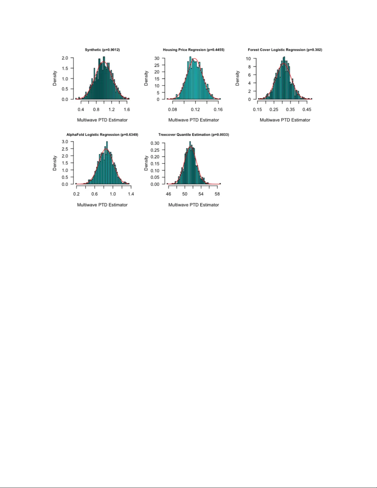
M-estimation under Tw o-Phase Multiw a v e Sampling with Applications to Prediction-P o w ered Inference Dan M. Kluger ∗ 1,2 and Stephen Bates 2 1 Institute for Data, Systems, and So ciet y , Massac husetts Institute of T ec hnology 2 Departmen t of Electrical Engineering and Computer Science, Massach usetts Institute of T echnology Abstract In tw o-phase multiw av e sampling, inexp ensiv e measurements are collected on a large sample and exp ensiv e, more informativ e measurements are adaptiv ely obtained on subsets of units across multiple w a ves. Adaptiv ely collecting the exp ensiv e measurements can increase eﬃciency but complicates statistical inference. W e giv e v alid estimators and conﬁdence interv als for M- estimation under adaptive tw o-phase multiw av e sampling. W e fo cus on the case where pro xies for the exp ensiv e v ariables—such as predictions from pretrained machine learning mo dels—are a v ailable for all units and prop ose a Multiwave Pr e dict-Then-Debias estimator that com bines pro xy information with the exp ensiv e, higher-quality measurements to improv e eﬃciency while remo ving bias. W e establish asymptotic linearity and normalit y and prop ose asymptotically v alid conﬁdence in terv als. W e also develop an appro ximately greedy sampling strategy that impro ves eﬃciency relativ e to uniform sampling. Data-based sim ulation studies support the theoretical results and demonstrate eﬃciency gains. Keyw ords: active inference, adaptiv e designs, M-estimation, tw o-phase multiw a ve sampling, Ney- man allo cation 1 In tro duction With recen t adv ances in mac hine learning and artiﬁcial in telligence, researchers are increasingly assem bling and analyzing large sample datasets in which some v ariables are algorithmic outputs rather than direct measuremen ts of the quantit y of interest. F or example, a study ma y use a predicted protein structure from a protein language mo del rather than a structure measured with crystallograph y , b ecause the latter is costly and time intensiv e. In this situation, naively applying traditional metho ds for statistical analysis will result in biased estimators and in v alid conﬁdence in terv als. Nonetheless, there is an emerging to ol kit of statistical metho ds that do w ork with suc h data, pro vided the analyst do es ha v e access to a small amount of gold standar d direct measuremen ts to complement algorithmic predictions (e.g., Angelop oulos et al., 2023a; Song et al., 2026). In this paper, we consider the v ersion of this problem where the researc her can adaptiv ely collect suc h gold standard measurements. This has the promise of increasing sample eﬃciency , resulting in narro wer conﬁdence in terv als for the parameter of interest with the same amount of data. A ma jor ∗ Corresp onding author: dkluger@mit.edu 1 tec hnical challenge is that adaptive sampling schemes can introduce statistical dep endencies across the samples, rendering it substantially more c hallenging to conduct v alid statistical inference. In this work, w e introduce a new estimator and conﬁdence in terv als for the adaptive setting and prov e their v alidit y . Our w ork can b e viewed as an instance of t wo-phase multiw a v e sampling (McIsaac and Co ok, 2015; Chen and Lumley, 2020, 2022) in which exp ensiv e v ariables are adaptively collected across m ultiple measurement w av es. While the literature on t wo-phase multiw a ve sampling also studies practical sampling strategies and estimators in the regime w e study , to our kno wledge this literature has not established asymptotic normalit y of M-estimators using theory that accounts for statistical dep endencies induced by the prop osed sampling strategies. Moreov er, muc h of the w ork in this literature assumes stratiﬁed sampling from pre-sp eciﬁed strata. In this pap er, w e consider more ﬂexible sampling strategies that do not require stratiﬁcation. Sim ultaneously , our w ork can also b e viewed as a part of the broader adaptiv e sampling and exp erimen tal design literature, and it is closely related to recent research on Activ e Statistical Inference (Zrnic and Candes, 2024). Giv en the diﬃculty of constructing asymptotically normal estimators in adaptiv e sampling settings, most studies restrict their attention to one of t wo simpler adaptiv e sampling regimes. The ﬁrst is a data splitting regime, in whic h the optimal sampling rule is estimated on an indep enden t pilot dataset and inference is conducted on the remaining data using standard asymptotic theory for i.i.d. samples. This leads to v alidit y , but loses p o wer since the pilot sample is discarded. The second sampling regime is online sampling: the data is observed in a sequence and the decision of whether to measure a data p oin t must b e made once and for all based on data collected up to that p oin t. This sampling scheme allo ws for the use of martingale tec hniques to construct conﬁdence in terv als. How ev er, a ma jor limitation of the online regime is that it do es not allow revisiting earlier samples if they are not measured. In contrast, in our work, if some particularly v aluable data p oin ts were not measured in early w av es, they are likely to still b e measured in later wa v es after a b etter estimate of the optimal sampling strategy is obtained. W e discuss related work in detail in Section 6. 1.1 Our con tribution W e in tro duce an estimator for the tw o-phase m ultiwa v e setting. W e prov e that this estimator is asymptotically linear and asymptotically normal, and use this to provide asymptotic conﬁdence in terv als. T o our knowledge, this is the ﬁrst approach to M-estimation in t wo-phase m ultiwa v e sampling with theoretical guarantees. W e also discuss how the user should c ho ose the sampling strategy for increased statistical eﬃciency . 1.2 Outline The outline of this pap er is as follo ws. In S ection 2, we introduce the formal setting and notation and describ e the p oin t estimator and its corresp onding conﬁdence interv als. In Section 3, we presen t our main theoretical results whic h (i) establish asymptotic linearity of the p oin t estimator in M- estimaton tasks under fairly mild conditions (ii) pro vide a central limit theorem for the p oin t estimator and (iii) establish conditions under which the conﬁdence interv als are asymptotically v alid. In Section 4, we use the asymptotic v ariance form ula obtained in the previous section to motiv ate sampling strategies that are designed to reduce asymptotic v ariance. In Section 5, we conduct sim ulations to test the empirical p erformance and cov erage of a few of these sampling strategies. In Section 6, we review related work. The pro ofs for all theoretical results are provided in the app endix. 2 2 Setting, p oin t estimator, and conﬁdence in terv al construction In this section, we formally in tro duce our notation and setting and describ e t wo-phase proxy- assisted m ultiwa v e sampling. W e then in tro duce appropriate in verse probability w eights that can b e used in these settings. F or M-estimation tasks, we prop ose a Predict-Then-Debias t yp e esti- mator (Chen and Chen, 2000; Kluger et al., 2025) that lev erages all av ailable data and presen t corresp onding conﬁdence interv als. Throughout the text, we supp ose V ≡ ( X c , ˜ X e , X e ) ∼ P V is a random v ector in R q in whic h X e denotes a v ector of exp ensiv e-to-measure v ariables, ˜ X e denotes a c heap-to-measure estimate of X e , and X c is a vector of other v ariables of interest or auxiliary v ariables that are also cheap-to- measure. W e use the shorthand notation X ≡ ( X c , X e ) ∈ R p to denote the vector of gold standard measuremen ts for all v ariables of in terest. It will also b e con v enient to let ˜ X ≡ ( X c , ˜ X e ) ∈ R p denote the cheap-to-measure vector of estimates for all v ariables of in terest. W e use X ⊆ R p and ˜ X ⊆ R p to denote the supp orts of X and ˜ X , resp ectiv ely , whic h satisfy P V ( X ∈ X ) = 1 = P V ( ˜ X ∈ ˜ X ). W e use P ≡ { π : ˜ X → (0 , 1) } to denote the space of p ossible lab eling rules (a lab elling rule maps ˜ X observ ations to a probabilit y that the corresp onding X e will b e measured). F or p ositiv e in tegers n w e use [ n ] = { 1 , . . . , n } to denote the set of the ﬁrst n p ositiv e integers. W e use S N =  τ : [ N ] → [ N ] suc h that τ is bijective  (that is S N is the collection of p erm utations of the ﬁrst N integers). W e use o p (1) to denote sequences that conv erge in probabilit y to 0 as N → ∞ and O p (1) to denote sequences that are b ounded in probabilit y as N → ∞ . With sligh t abuse of notation, for each p ositiv e integer j w e let e j denote the j th standard basis v ector in R d ∗ whose dimension d ∗ dep ends on the context. Unless otherwise sp eciﬁed, sums and pro ducts o ver ranges of indices in which the low er limit exceeds the upp er limit are deﬁned to b e 0 and 1, resp ectiv ely . 2.1 Tw o-phase pro xy-assisted m ultiwa v e sampling In tw o-phase proxy-assisted m ultiwa v e sampling, Phase I inv olv es collecting a large sample of size N in whic h the less exp ensiv e v ariables ˜ X = ( X c , ˜ X e ) are measured for eac h sample but mea- suremen t of the exp ensiv e v ariable X e is reserved for Phase I I. Phase I I in volv es K w a ves. In eac h w av e, X e i measuremen ts are collected on a subset of the N samples using indep enden t Bernoulli sampling. The probability that an X e i measuremen t is collected is a function of the av ailable data for the i th sample ˜ X i = ( X c i , ˜ X e i ) and a lab elling rule that is learned on data from previous wa v es. The procedure, which we refer to as t wo-phase proxy-assisted multiw a v e sampling is formally stated in the b o x b elo w, with elab orations and assumptions ab out eac h step subsequen tly provided. Tw o-phase proxy-assisted m ultiwa v e sampling sc heme Phase I (Inexp ensiv e v ariable collection): Collect an i.i.d. sample of size N from the sup erpopulation. F or each i ∈ [ N ], observe the inexp ensiv e v ariables ˜ X i = ( X c i , ˜ X e i ), while the exp ensiv e v ariable X e i remains unobserved. Data av ailable after Phase I is denoted by D 0 ≡ ( ˜ X i ) N i =1 . Phase I I (Adaptive m ultiwa v e measuremen ts): F or wa ves k = 1 , . . . , K : 1. Learn lab elling rule: Use all data collected prior to w av e k , denoted by D k − 1 , and apply the lab elling strategy A ( k ) π to obtain a lab elling rule π ( k ) D k − 1 = A ( k ) π ( D k − 1 ) ∈ P . 3 2. Select units for measurement: F or each i ∈ [ N ], compute the lab elling probability π ( k ) D k − 1 ( ˜ X i ) . Dra w U ( k ) i i.i.d. ∼ Unif [0 , 1] indep enden tly of D k − 1 and set I ( k ) i ≡ 1 { U ( k ) i ⩽ π ( k ) D k − 1 ( ˜ X i ) } . 3. Collect measuremen ts: Observe X e i if b oth I ( k ) i = 1 and X e i has not b een previously measured. Data av ailable after wa v e k is denoted by D k ≡  ( I ( j ) i , I ( j ) i X e i ) k j =1 , ˜ X i  N i =1 . Observ ed data after Phase I I: The resulting dataset (and other sampling information that is helpful to store for estimation and inference) is denoted b y D out ≡   I ( j ) i , U ( j ) i , π ( j ) D j − 1 ( ˜ X i )  K j =1 , ˜ X i , I i X e i  N i =1 , where I i ∈ { 0 , 1 } is an indicator of whether X e i w as measured in an y of the K wa ves. W e now elab orate on assumptions and implementation requirements for speciﬁc steps within t wo-phase proxy-assisted multiw a ve sampling. In Phase I, we assume that the N samples collected are i.i.d. from the sup erp opulation of in terest. While the X e i v alues are unobserv ed in Phase I, the following assumption states that the data would b e an i.i.d. sample if X e i w ere collected for all Phase I samples. Assumption 1 (i.i.d. Phase I samples) . V 1 , . . . , V N i.i.d. ∼ P V , where V i ≡ ( X c i , ˜ X e i , X e i ) for i ∈ [ N ]. In each wa v e k in Phase I I, the lab elling strategy A ( k ) π is a presp eciﬁed function that maps all previously observ ed data (and sampling indicators), denoted b y D k − 1 , to a lab elling rule in P ≡ { π : ˜ X → (0 , 1) } . If the labelling rule π ∈ P is selected, then for each i ∈ [ N ], X e i is to b e measured with probability π ( ˜ X i ) according to indep enden t Bernoulli sampling. If X e i has already b een measured in a previous wa v e, a measurement of it is not collected again (for simplicity , we consider settings where X e i can b e measured without noise so rep eated measurements are of no v alue). W e also supp ose that the presp eciﬁed lab elling strategy A ( k ) π is suﬃciently regular to not in tro duce measurabilit y concerns (more sp eciﬁcally , for eac h i ∈ [ N ] and k ∈ [ K ] w e assume that the w av e k lab eling probabilities for sample i , given b y [ A ( k ) π ( D k − 1 )]( ˜ X i ) can b e expressed as a measurable function of D k − 1 and ˜ X i ). Exploration of lab elling strategies A ( k ) π that result in eﬃcien t estimation of the parameter of interest is deferred to Section 4. 2.2 Multiw a ve in verse probabilit y weigh ts W e next in tro duce in verse probabilit y-type weigh ts that are appropriate for tw o-phase m ultiwa v e sampling settings. F or each i ∈ [ N ], and k ∈ { 2 , . . . , K } , deﬁne W ( k ) i ≡  k − 1 Y j =1 1 − I ( j ) i 1 − π ( j ) D j − 1 ( ˜ X i )  I ( k ) i π ( k ) D k − 1 ( ˜ X i ) , (1) and W (1) i ≡ I (1) i /π (1) D 0 ( ˜ X i ) for i ∈ [ N ]. W e next aggregate the weigh ts across the K wa v es. In particular, ﬁx c 1 , c 2 , . . . , c K ∈ [0 , 1] such that P K k =1 c k = 1, and deﬁne the following multiw a ve 4 in verse probability weigh ts W i ≡ K X k =1 c k W ( k ) i for all i ∈ [ N ] . (2) The presp eciﬁed c k determine ho w muc h weigh t should b e given to each wa ve, and as a starting p oin t can b e made prop ortional to the exp ected size of each wa v e. W e remark that these weigh ts are not the same as those seen in some other works on tw o-phase m ultiwa v e sampling (Chen et al., 2025b; Y ang et al., 2022). In those works the inv erse probability w eights are giv en by calculating the total probability of a sample b eing labelled ov er the course of all wa v es. Our construction of the w eigh ts enables us to establish theoretical guarantees by recursiv e applications of the to wer prop ert y where we condition on data from previous w av es. W e exp ect that some prop erties of the multiw av e inv erse probability weigh ts W i , such as their lack of pairwise correlations, may b e useful in other contexts, and we record them in App endix A. 2.3 Multiw a ve Predict-Then-Debias M-estimator Our fo cus is on M-estimation settings where there is some presp eciﬁed loss function l θ : R p → R parameterized by θ ∈ Θ ⊆ R d and the goal is to estimate the well-deﬁned quantit y of in terest θ 0 ≡ arg min θ ∈ Θ E [ l θ ( X )] . (3) As examples, the loss function l θ ( · ) could be chosen such that θ 0 is a population mean, a p opulation quan tile, or a p opulation regression co eﬃcien t in a GLM or robust regression mo del that regresses one comp onen t of X on other comp onen ts of X . W e b egin with 3 simple estimators (the ﬁrst tw o of which use Phase I I information): ˆ θ II ≡ arg min θ ∈ Θ 1 N N X i =1 W i l θ ( X i ) , ˆ γ II ≡ arg min θ ∈ Θ 1 N N X i =1 W i l θ ( ˜ X i ) , and ˆ γ I ≡ arg min θ ∈ Θ 1 N N X i =1 l θ ( ˜ X i ) . (4) W e then combine these estimators into our prop osed Multiwave Pr e dict-Then-Debias estimator ˆ θ MPD = ˆ Ω ˆ γ I + ( ˆ θ II − ˆ Ω ˆ γ II ) , (5) where ˆ Ω ∈ R d × d is a tuning parameter for impro ved eﬃciency that we will discuss in due course. The reader can keep in mind the case where ˆ Ω is the identit y matrix as an intuitiv e sp ecial case. The idea b ehind the estimator is as follo ws. The estimator ˆ θ II minimizes an empirical weigh ted loss whose exp ected v alue is E [ l θ ( X )] (see Prop osition A.4 in the App endix for details), so ˆ θ II is an estimator targeting the estimand of in terest θ 0 . Likewise, ˆ γ II and ˆ γ I minimize empirical loss functions whose exp ected v alues are E [ l θ ( ˜ X )], so these estimators target the quantit y γ 0 ≡ arg min θ ∈ Θ E [ l θ ( ˜ X )] . Imp ortan tly , γ 0 is generally not equal to θ 0 , since the distribution of ˜ X is not the same as that of X . Still, ˆ γ I has low v ariance b ecause it is based on all N samples, so it is useful to anc hor on this quan tity . Then, we add a bias-correction term such that the resulting estimator targets θ 0 . In this manuscript, we will show that this estimator is consistent and asymptotically normal. Moreo ver, it results in improv ed eﬃciency compared to baseline approac hes such as ˆ θ II and other non-adaptiv e strategies. W e will also give a consisten t v ariance estimator, which leads to v alid conﬁdence in terv als. 5 2.4 Asymptotic v ariance estimator and conﬁdence in terv als A formula for the asymptotic v ariance of ˆ θ MPD will subsequently b e given in Theorem 3, and w e state a consisten t v ariance estimator here. Deﬁne the follo wing: ˆ Σ 11 ≡ 1 N N X i =1 W 2 i ˙ l ˆ θ II ( Y i )[ ˙ l ˆ θ II ( X i )] T , ˆ Σ 12 ≡ 1 N N X i =1 W 2 i ˙ l ˆ θ II ( X i )[ ˙ l ˆ γ I ( ˜ X i )] T , ˆ Σ 22 ≡ 1 N N X i =1 W 2 i ˙ l ˆ γ I ( ˜ X i )[ ˙ l ˆ γ I ( ˜ X i )] T , ˆ Σ 13 ≡ 1 N N X i =1 W i ˙ l ˆ θ II ( X i )[ ˙ l ˆ γ I ( ˜ X i )] T , ˆ Σ 33 ≡ 1 N N X i =1 ˙ l ˆ γ I ( ˜ X i )[ ˙ l ˆ γ I ( ˜ X i )] T , ˆ H θ 0 ≡ 1 N N X i =1 W i ¨ l ˆ θ II ( X i ) , and ˆ H γ 0 ≡ 1 N N X i =1 ¨ l ˆ γ I ( ˜ X i ) . (6) Ab o v e for eac h x ∈ X ∪ ˜ X and θ ′ ∈ Θ, ˙ l θ ′ ( x ) and ¨ l θ ′ ( x ) denote the gradient and Hessian, resp ectiv ely , of the map θ 7→ l θ ( x ) ev aluated at θ = θ ′ . (W e remark that in some cases θ 7→ l θ is not diﬀerentiable or t wice diﬀerentiable at θ = ˆ θ II or θ = ˆ γ I , in which case the cov ariance matrices in (6) ma y not b e clearly deﬁned. In such cases w e deﬁne ˙ l θ ′ ( x ) and ¨ l θ ′ ( x ) in terms of the ﬁrst and second order upp er righ t-hand Dini partial deriv ativ es to ensure that the ab o ve estimators are w ell-deﬁned). Letting ˆ Ω ∈ R d × d b e the (p ossibly data dep enden t) tuning matrix used to construct ˆ θ MPD , an estimator for the asymptotic v ariance of ˆ θ MPD is then given by ˆ Σ MPD ≡ ˆ H − 1 θ 0 ˆ Σ 11 ˆ H − 1 θ 0 + ˆ Ω ˆ H − 1 γ 0  ˆ Σ 22 − ˆ Σ 33  ˆ H − 1 γ 0 ˆ Ω T + ˆ H − 1 θ 0 ( ˆ Σ 13 − ˆ Σ 12 ) ˆ H − 1 γ 0 ˆ Ω T +  ˆ H − 1 θ 0 ( ˆ Σ 13 − ˆ Σ 12 ) ˆ H − 1 γ 0 ˆ Ω T  T . (7) Tw o-sided (1 − α )-conﬁdence interv als for the j th comp onen t of θ 0 are then given by C (1 − α ) j ≡ h ˆ θ MPD j − z 1 − α/ 2 q ˆ Σ MPD j j / N , ˆ θ MPD j + z 1 − α/ 2 q ˆ Σ MPD j j / N i for each j ∈ [ d ] , α ∈ (0 , 1) , (8) where abov e z 1 − α/ 2 denotes the (1 − α/ 2)-th quantile of a standard normal distribution. Un- der certain assumptions, this v ariance estimator is consisten t and these conﬁdence interv als are asymptotically v alid; we turn to the technical details next. 3 Asymptotic theory In this section, we study the asymptotic properties of the estimator ˆ θ MPD under tw o-phase pro xy-assisted multiw a ve sampling. In particular, we show that under relativ ely mild regularity conditions, ˆ θ MPD is consistent and asymptotically linear. Here the asymptotic linear expansion in volv es statistically dep enden t w eights ( W i ) N i =1 . Under additional assumptions, we establish that ˆ θ MPD is asymptotically normal. Finally , under additional regularity conditions w e show that the conﬁdence in terv als deﬁned at (8) are asymptotically v alid. 3.1 Consistency , √ N -consistency , and asymptotic linearity W e b egin b y requiring that the probabilities π ( k ) D k − 1 ( ˜ X i ) are b ounded aw a y from zero and one, as is commonplace. Assumption 2 . There exists a constant b ∈ (0 , 1 / 2) that do es not dep end on N suc h that almost surely π ( k ) D k − 1 ( ˜ X i ) ∈ [ b, 1 − b ] for each k ∈ [ K ] and i ∈ [ N ]. 6 The constant b may b e arbitrarily close to 0, but may not decrease as N → ∞ . In our setting, w e ha ve the capabilit y to ensure that this assumption holds, since w e con trol the lab elling probabilities. Next, w e require regularity conditions of the loss function to enable M-estimation. In particular, for eac h θ ∈ Θ deﬁne L ( θ ) ≡ E [ l θ ( X )] and ˜ L ( θ ) ≡ E [ l θ ( ˜ X )] to b e the p opulation losses and we supp ose that the loss l θ ( · ) satisﬁes the following conditions. Assumption 3 (Regularity conditions for M-estimation) . (i) θ 7→ l θ ( x ) is conv ex for every x ∈ X ∪ ˜ X . (ii) Across the domain Θ, θ 0 is the unique minimizer of L ( θ ) and γ 0 is the unique minimizer of ˜ L ( θ ) with θ 0 and γ 0 b eing in the interior of set Θ. (iii) θ 7→ l θ ( x ) is diﬀerentiable at θ = θ 0 for all x ∈ X and θ 7→ l θ ( ˜ x ) is diﬀerentiable at θ = γ 0 for all ˜ x ∈ ˜ X . (iv) θ 7→ l θ ( X ) is lo cally Lipsc hitz around θ = θ 0 and θ 7→ l θ ( ˜ X ) is lo cally Lipsc hitz around θ = γ 0 . In particular, there exists neighborho ods L θ 0 of θ 0 and L γ 0 of γ 0 , and there exists functions M , ˜ M : R p → (0 , ∞ ) such that E [ M 2 ( X )] < ∞ , E [ ˜ M 2 ( ˜ X )] < ∞ , and such that for all x ∈ X and θ, θ ′ ∈ L θ 0 , | l θ ( x ) − l θ ′ ( x ) | < M ( x ) || θ − θ ′ || while for all ˜ x ∈ ˜ X and θ , θ ′ ∈ L γ 0 , | l θ ( ˜ x ) − l θ ′ ( ˜ x ) | < ˜ M ( ˜ x ) || θ − θ ′ || . (v) The p opulation losses giv en by L ( θ ) and ˜ L ( θ ) b oth admit a 2nd-order T a ylor expansions ab out θ 0 and γ 0 , resp ectiv ely , and the Hessians ∇ 2 L ( θ 0 ) and ∇ 2 ˜ L ( γ 0 ) are nonsingular. (vi) E [ l 2 θ 0 ( X )] < ∞ and E [ l 2 γ 0 ( ˜ X )] < ∞ . The ab o ve assumptions are fairly standard in M-estimation theory (e.g, v an der V aart (1998); Angelop oulos et al. (2023c)), ev en when the data are an i.i.d. sample rather than our more chal- lenging adaptiv e sampling setting. Under Assumption 3, deﬁne H θ 0 ≡ ∇ 2 L ( θ 0 ) = ∇ 2 θ E [ l θ ( X )]   θ = θ 0 , H γ 0 ≡ ∇ 2 ˜ L ( γ 0 ) = ∇ 2 θ E [ l θ ( ˜ X )]   θ = γ 0 , and ˙ l θ ′ ( x ) ≡ ∇ θ l θ ( x )   θ = θ ′ , where the ﬁnal quan tity is deﬁned for any x ∈ R p and θ ′ ∈ Θ such that θ 7→ l θ ( x ) is diﬀerentiable at θ = θ ′ . Under Assumption 3(v), H θ 0 and H γ 0 exist and are in vertible while under Assumption 3(iii), ˙ l θ 0 ( X ) and ˙ l γ 0 ( ˜ X ) exist almost surely . Assumptions 1, 2, and 3 are suﬃcien t to ensure that ˆ θ II , ˆ γ II , and ˆ γ I are each √ N -consisten t estimators for θ 0 , γ 0 , and γ 0 resp ectiv ely , and that they each admit asymptotic linear expansions. Theorem 1. Under two-phase pr oxy-assiste d multiwave sampling and Assumptions 1, 2, and 3, √ N   ˆ θ II ˆ γ II ˆ γ I   −   θ 0 γ 0 γ 0   ! = − 1 √ N N X i =1   H − 1 θ 0 0 0 0 H − 1 γ 0 0 0 0 H − 1 γ 0     W i ˙ l θ 0 ( X i ) W i ˙ l γ 0 ( ˜ X i ) ˙ l γ 0 ( ˜ X i )   + o p (1) . Mor e over, the ab ove ar e O p (1) . As a corollary , in the setting of Theorem 1, ˆ θ MPD is consistent for θ 0 and asymptotically linear, pro vided that the ˆ Ω conv erges in probabilit y as N → ∞ . 7 Corollary 2. Under two-phase pr oxy-assiste d multiwave sampling and Assumptions 1, 2, and 3, and if the tuning matrix ˆ Ω p − → Ω as N → ∞ , ˆ θ MPD p − → θ 0 as N → ∞ and √ N  ˆ θ MPD − θ 0  = − 1 √ N N X i =1  W i H − 1 θ 0 ˙ l θ 0 ( X i ) + (1 − W i )Ω H − 1 γ 0 ˙ l γ 0 ( ˜ X i )  + o p (1) . (9) This conclusion ab out ˆ θ MPD is the asp ect of this section of most metho dological in terest. W e will next lev erage this result to prov e asymptotic normality , but ﬁrst we pause to comment on the tec hnical challenges b ehind the ab o ve result. Theorem 1 and it’s proof make up a ma jor technical contribution of this pap er. Asymptotic linearit y is common in i.i.d. settings, but extending it to the adaptive setting is delicate. In particular, in App endix B.3 w e use similar symmetrization and chaining arguments for empirical pro cesses as seen in canonical texts suc h as v an der V aart (1998); V ershynin (2018) and v an der V aart and W ellner (2023). In contrast to these, ho wev er, we decomp ose empirical weigh ted pro cesses in to m ultiple terms, each of which can b e controlled b y symmetrization arguments when conditioning on data from prior wa v es by lev eraging conditional indep endencies of the form I ( k ) i | = I ( k ) i ′ | D k − 1 for i  = i ′ . Our mo diﬁed symmetrization and chaining argumen ts also leverage the b oundedness of the w eights (Assumption 2) to establish that exp ected ﬂuctuations of the relev an t lo cal empirical pro cesses are still controlled at a suﬃcien tly fast rate in our dep endency regime. 3.2 Asymptotic normalit y W e next turn to asymptotic normality . Under nonadaptive sampling, an asymptotic linear ex- pansion such as the one in Corollary 2 together with the central limit theorem (CL T) and Slutsky’s immediately establish asymptotic normalit y . Ho wev er, in t wo-phase pro xy-assisted multiw a ve sam- pling, the standard m ultiv ariate central limit cannot b e applied b ecause the terms b eing av eraged are not statistically indep enden t. W e introduce additional assumptions that are suﬃcien t to ensure that ˆ θ MPD is asymptotically normal. Assumption 4 (Regularity conditions for establishing asymptotic normality) . (i) Symmetric lab el ling str ate gies. F or each k ∈ { 0 } ∪ [ K ] and p erm utation τ ∈ S N , let D ( τ ) k ≡  ( I ( j ) τ ( i ) , I ( j ) τ ( i ) · X e τ ( i ) ) k j =1 , ˜ X τ ( i )  N i =1 denote a p erm utation of the data that is a v ailable after the k th w av e according to the p erm utation τ . Recall A ( k ) π ( D k − 1 ) ∈ P is a mapping ˜ X → (0 , 1). F or eac h k ∈ [ K ] and permutation τ ∈ S N , π ( k ) D k − 1 ≡ A ( k ) π ( D k − 1 ) = A ( k ) π ( D ( τ ) k − 1 ). (ii) L 1 c onver genc e of lab el ling rules . F or each k ∈ [ K ] there exists a measurable function ¯ π ( k ) : ˜ X → [ b, 1 − b ], such that lim N →∞ E  | π ( k ) D k − 1 ( ˜ X 1 ) − ¯ π ( k ) ( ˜ X 1 ) |  = 0 . (iii) Bounde d moments of or der gr e ater than 2. There exists an η ∗ > 0, such that for each j ∈ [ d ], E    [ ˙ l θ 0 ( X )] j   2+ η ∗  < ∞ and E    [ ˙ l γ 0 ( ˜ X )] j   2+ η ∗  < ∞ . Assumption 4(i) can b e ensured b y an in vestigator who is c ho osing a lab elling strategy , and will hold if the adaptive labelling strategy only giv es preference based on the v alues of the data that w as previously observ ed rather than the particular index of each sample. W e remark that Assumption 4(i) is not strictly necessary and can be remov ed if Assumption 4(ii) is strengthened to state that lim N →∞ sup i ∈ [ N ] E  | π ( k ) D k − 1 ( ˜ X i ) − ¯ π ( k ) ( ˜ X i ) |  = 0. Assumption 4(ii) is a fairly common condition requiring that the lab elling rules from eac h w av e conv erge as N → ∞ . If we are in an asymptotic 8 regime where the n umber of w av es remains ﬁxed as N → ∞ the lab elling strategies can be carefully c hosen so that this assumption holds (e.g., using parametric or consisten t nonparametric approaches to learn a go o d labelling rule). Notably , the L 1 con vergence of the lab elling rule can happ en at an y arbitrarily slo w rate, while other theoretical results in the adaptive exp erimen t literature (e.g., Hahn et al. (2011); Li and Owen (2024); Nw ankwo et al. (2025)) assume particular rates of conv ergence. In order to present a formula for the asymptotic v ariance of ˆ θ MPD it is conv enien t to deﬁne ¯ π (1: k ) ( ˜ x ) ≡ ¯ π ( k ) ( ˜ x ) k − 1 Y j =1  1 − ¯ π ( j ) ( ˜ x )  for k ∈ [ K ] , ˜ x ∈ ˜ X . (10) The ab o ve quantit y can b e thought of as a limiting probabilit y of a sample with cheap-to-measure data ˜ x b eing selected for lab elling in the k th wa v e, but not in previous w av es. Deﬁne also Σ 11 ≡ K X k =1 c 2 k E h ˙ l θ 0 ( X )[ ˙ l θ 0 ( X )] T ¯ π (1: k ) ( ˜ X ) i , Σ 12 ≡ K X k =1 c 2 k E h ˙ l θ 0 ( X )[ ˙ l γ 0 ( ˜ X )] T ¯ π (1: k ) ( ˜ X ) i , Σ 13 ≡ E  ˙ l θ 0 ( X )[ ˙ l γ 0 ( ˜ X )] T  , Σ 22 ≡ K X k =1 c 2 k E h ˙ l γ 0 ( ˜ X )[ ˙ l γ 0 ( ˜ X )] T ¯ π (1: k ) ( ˜ X ) i , and Σ 33 ≡ E  ˙ l γ 0 ( ˜ X )[ ˙ l γ 0 ( ˜ X )] T  . (11) F or an y ﬁxed tuning matrix Ω ∈ R d × d , the asymptotic v ariance is then Σ MPD (Ω) ≡ H − 1 θ 0 Σ 11 H − 1 θ 0 + Ω H − 1 γ 0  Σ 22 − Σ 33  H − 1 γ 0 Ω T + H − 1 θ 0 (Σ 13 − Σ 12 ) H − 1 γ 0 Ω T +  H − 1 θ 0 (Σ 13 − Σ 12 ) H − 1 γ 0 Ω T  T . (12) Theorem 3. Under two-phase pr oxy-assiste d multiwave sampling and Assumptions 1,2, 3, and 4, if ˆ Ω p − → Ω , √ N ( ˆ θ MPD − θ 0 ) d − → N  0 , Σ MPD (Ω)  as N → ∞ . The main pro of strategy is to introduce weigh ts that are b oth (i) statistically indep enden t of eac hother and (ii) asymptotically close enough to the statistically dep enden t w eights ( W i ) N i =1 . Up to o p (1) terms, the asymptotic linear expansion in Corollary 2 can then b e rewritten in terms of these statistically indep enden t weigh ts, enabling the application of the standard m ultiv ariate cen tral limit theorem. 3.3 Conﬁdence in terv al v alidit y T o establish asymptotic v alidity of the conﬁdence interv als using the previous asymptotic nor- malit y result, it remains to establish that the asymptotic cov ariance estimator at (7) is consisten t. T o ensure consistent asymptotic cov ariance matrix estimation, we introduce the following assump- tions on the loss function l θ ( · ). Assumption 5 (Regularity conditions for consistent v ariance estimation) . (i) θ 7→ l θ ( x ) is c ontinuously twice diﬀerentiable at θ = θ 0 for all x ∈ X while θ 7→ l θ ( ˜ x ) is c ontinuously twice diﬀerentiable at θ = γ 0 for all ˜ x ∈ ˜ X . Moreo ver, the loss is smo oth enough suc h that 2nd deriv atives and expectations can b e swapped so that E [ ¨ l θ 0 ( X )] = H θ 0 and E [ ¨ l γ 0 ( ˜ X )] = H γ 0 . 9 (ii) F or each j, j ′ ∈ [ d ] there exists functions L j j ′ , ˜ L j j ′ : R p → [0 , ∞ ] satisfying E [ L j j ′ ( X )] < ∞ and E [ ˜ L j j ′ ( ˜ X )] < ∞ as well as a neighborho o d B j j ′ of θ 0 and a neighborho o d ˜ B j j ′ of γ 0 , such that | [ ¨ l θ ( x )] j j ′ | ≤ L j j ′ ( x ) for all θ ∈ B j j ′ and x ∈ X , and | [ ¨ l θ ( ˜ x )] j j ′ | ≤ ˜ L j j ′ ( ˜ x ) for all θ ∈ ˜ B j j ′ and ˜ x ∈ ˜ X . (iii) F or eac h j, j ′ ∈ [ d ], E  [ ¨ l θ 0 ( X )] j j ′  2  < ∞ , E  [ ˙ l θ 0 ( X )] j  4  < ∞ , and E  [ ˙ l γ 0 ( ˜ X )] j  4  < ∞ . The abov e assumptions are all smo othness and b ounded moment conditions on the ﬁrst and second deriv ativ es of θ 7→ l θ ( X ) and θ 7→ l θ ( ˜ X ) in neighborho ods of θ 0 and γ 0 , resp ectiv ely . They are suﬃcient, although p erhaps not necessary , for establishing the consistency estimators deﬁned at (6) in the following sense. Prop osition 4. Under two-phase pr oxy-assiste d multiwave sampling and Assumptions 1, 2, 3, 4, and 5, ˆ Σ 11 p − → Σ 11 , ˆ Σ 12 p − → Σ 12 , ˆ Σ 22 p − → Σ 22 , ˆ Σ 13 p − → Σ 13 , ˆ Σ 33 p − → Σ 33 , ˆ H θ 0 p − → H θ 0 , and ˆ H γ 0 p − → H γ 0 as N → ∞ . T o b e in the setting of Theorem 3, we need to c ho ose a tuning matrix ˆ Ω such that ˆ Ω p − → Ω for some Ω ∈ R d × d . A fairly general w ay to choose the tuning matrix is to tak e it to b e some function of the empirical matrices ab o ve: ˆ Ω = f  ˆ Σ 11 , ˆ Σ 12 , ˆ Σ 22 , ˆ Σ 13 , ˆ Σ 33 , ˆ H θ 0 , ˆ H γ 0  for some f : ( R d × d ) 7 → R d × d . (13) It will also b e con venien t to deﬁne Ω f ≡ f  Σ 11 , Σ 12 , Σ 22 , Σ 13 , Σ 33 , H θ 0 , H γ 0  for each f : ( R d × d ) 7 → R d × d . (14) By the con tinuous mapping theorem and Proposition 4, if ˆ Ω satisﬁes (13) for some function f that is con tinuous at (Σ 11 , Σ 12 , Σ 22 , Σ 13 , Σ 33 , H θ 0 , H γ 0 ), ˆ Ω conv erges in probabilit y to Ω f ∈ R d × d . W e can th us combine Theorem 3 and Prop osition 4 to get the following result, which establishes asymptotically v alid conﬁdence in terv als for θ 0 . Prop osition 5. Supp ose the data ar e c ol le cte d via two-phase pr oxy-assiste d multiwave sampling, that Assumptions 1, 2, 3, 4, and 5 hold and that ˆ θ MPD is tune d using a tuning matrix ˆ Ω given by (13) for some f : ( R d × d ) 7 → R d × d that is c ontinuous at (Σ 11 , Σ 12 , Σ 22 , Σ 13 , Σ 33 , H θ 0 , H γ 0 ) . Then, ˆ Σ MPD p − → Σ MPD (Ω f ) as N → ∞ , wher e ˆ Σ MPD , Σ MPD ( · ) , and Ω f , ar e deﬁne d at Equations (7) , (12) , and (14) , r esp e ctively. Mor e over, if Σ MPD (Ω f ) ≻ 0 , then lim N →∞ P  [ θ 0 ] j ∈ C (1 − α ) j  = 1 − α for e ach j ∈ [ d ] , α ∈ (0 , 1) , wher e C (1 − α ) j denotes the (1 − α ) -c onﬁdenc e interval for the j th c omp onent of θ 0 deﬁne d at (8) . 4 Cho osing sampling rules to increase eﬃciency The app eal of t wo-phase m ultiwa v e sampling is that w e can choose to sample p oin ts that are most informativ e, increasing eﬃciency . In particular, sampling in multiple w av es allo ws us to adaptiv ely up date our sampling strategy as w e acquire more data and b etter understand which future data is likely to b e most b eneﬁcial. W e no w turn our attention to the lab eling strategy A ( k ) π for each k ∈ [ K ], discussing c hoices that lead to impro ved eﬃciency . Subsequen tly , w e brieﬂy discuss the choice of the tuning matrix ˆ Ω and weigh ts c 1 , . . . , c K ∈ [0 , 1]. 10 4.1 An appro ximate greedy optimal strategy In this subsection, w e present a strategy to for sampling in each wa v e that is designed to increase precision. W e fo cus on settings where the inv estigator is primarily in terested in a design that will lead to narrow conﬁdence interv als for the j th comp onen t of θ 0 for some ﬁxed j ∈ [ d ]. (Other ob jectives can b e considered in our framework but are omitted due to space constraints. See Y ang et al. (2025b) which studies A-optimalit y and Li and Ow en (2024) whic h studies more general information functions in related settings). F or simplicity , w e develop eﬃcien t designs for the case where c 1 , . . . , c K are ﬁxed and presp eciﬁed and the tuning matrix ˆ Ω = I d × d . Fix j ∈ [ d ]. T o state the asymptotic v ariance of ˆ θ MPD j when ˆ Ω = I d × d , it helps to deﬁne Σ c ≡  H − 1 θ 0 − H − 1 γ 0  T  0 Σ 13 Σ T 13 Σ 33   H − 1 θ 0 − H − 1 γ 0  and to deﬁne ψ j : X × ˜ X → R to b e a function given by ψ j ( x, ˜ x ) ≡  e T j H − 1 θ 0 ˙ l θ 0 ( x ) − e T j H − 1 γ 0 ˙ l γ 0 ( ˜ x )  2 for each x ∈ X , ˜ x ∈ ˜ X . (15) In the setting of Theorem 3, for any k ∗ ∈ [ K ], the asymptotic v ariance of ˆ θ MPD j is given by  Σ MPD ( I d × d )  j j = c 2 k ∗ E " ψ j ( X , ˜ X ) ¯ π (1: k ∗ ) ( ˜ X ) # + K X k ′ = k ∗ +1 c 2 k ′ E " ψ j ( X , ˜ X ) ¯ π (1: k ′ ) ( ˜ X ) # | {z } Depends on A ( k ) π for k > k ∗ + k ∗ − 1 X k ′ =1 c 2 k ′ E " ψ j ( X , ˜ X ) ¯ π (1: k ′ ) ( ˜ X ) # − [Σ c ] j j | {z } Does not depend on A ( k ∗ ) π choice . Note that b y (11) the matrix Σ c do es not dep end on the lab eling strategies {A ( k ) π } K k =1 or the limiting lab elling rules { ¯ π ( k ) } K k =1 , so the matrix Σ c can b e ignored when studying sampling strategies {A ( k ) π } K k =1 that w ould be eﬃcien t. W e next consider lab elling strategies for minimizing the asymptotic v ariance ab ov e in a greedy manner. In particular, ﬁx k ∗ ∈ [ K ] such that k ∗ ≥ 2. W e supp ose that the inv estigator will c ho ose their labelling strategy A ( k ∗ ) π for the k ∗ th w av e to minimize asymptotic v ariance in a scenario where the k ∗ th wa v e is last wa v e. Note that the choice of lab elling strategy A ( k ∗ ) π do es not inﬂuence the quan tities ¯ π (1: k ′ ) ( ˜ X ) in the abov e equation for k ′ < k ∗ whereas the terms with ¯ π (1: k ′ ) ( ˜ X ) for k ′ > k ∗ dep end on lab elling strategies after the k ∗ th wa v e and w ould not app ear in the ab ov e formula had the k ∗ th wa v e b een the last one. Th us when c ho osing the lab eling strategy A ( k ∗ ) π for the k ∗ th wa v e, the last tw o terms can b e completely ignored. Mean while, the 2nd term is ignored in a greedy approac h that assumes the k ∗ th wa v e will b e the last one. Recalling formula (10) and noting that c k ∗ ≥ 0 and all but the last term in the ab ov e v ariance decomp osition are ignored in a greedy optimization setting, we supp ose that the inv estigator c ho oses the lab elling strategy A ( k ∗ ) π with the goal of achieving a near optimal solution to the optimization problem ﬁnd a ¯ π ( k ∗ ) : R p → (0 , ∞ ) minimizing E " ψ j ( X , ˜ X ) Q k ∗ − 1 k =1  1 − ¯ π ( k ) ( ˜ X )  − 1 ¯ π ( k ∗ ) ( ˜ X ) # sub ject to E [ ¯ π ( k ∗ ) ( ˜ X )] ≤ B k ∗ and ¯ π ( k ∗ ) ( ˜ x ) ∈ [ b, 1 − b ] for ˜ x ∈ ˜ X . (16) 11 Ab o ve B k ∗ imp oses a budget constrain t on the exp ected n umber of lab els that can b e collected in the k ∗ th w av e and b ∈ (0 , 1 / 2) is an ov erlap b ound that constrains the search to lab elling rules that will satisfy Assumption 2. As in (Zrnic and Candes, 2024; Chen et al., 2025b) we now relax the constraint on the range of ¯ π ( k ∗ ) ( · ) to b e a nonnegativit y constrain t. Ignoring this b oundedness constrain t then corresp onds to an optimization problem with a solution that has app eared in the imp ortance sampling literature (Kahn and Marshall, 1953; Ow en, 2013) (we state and re-derive this with our notation in Lemma E.1 in the app endix). In particular, replacing the constraint that ¯ π ( k ∗ ) ( ˜ x ) ∈ [ b, 1 − b ] with a weak er restriction that ¯ π ( k ∗ ) ( ˜ x ) ∈ (0 , ∞ ) for ˜ x ∈ ˜ X , the solution to the optimization problem at (16) has an optimal ¯ π ( k ∗ ) ( · ) giv en b y ¯ π ( k ∗ ) opt ( ˜ X ) ∝ s ϱ j ( ˜ X ) Q k ∗ − 1 k =1  1 − ¯ π ( k ) ( ˜ X )  , where ϱ j ( ˜ X ) ≡ E [ ψ j ( X , ˜ X ) | ˜ X ] , (17) and where ¯ π ( k ∗ ) opt ( · ) is scaled by a prop ortionalit y constant so that E [ ¯ π ( k ∗ ) opt ( ˜ X )] = B k ∗ . F or a ﬁxed k ∗ ∈ [ K ] such that k ∗ ≥ 2, w e consider a lab elling strategy that would result in a labelling rule π ( k ∗ ) D k ∗ − 1 ( · ) rule that approximates ¯ π ( k ∗ ) opt ( · ), while satisfying budget and o verlap constrain ts. In particular, for eac h ˜ x ∈ ˜ X , let ˆ ¯ π ( k ∗ ) opt,init ( ˜ x ) = q ˆ ϱ j ( ˜ x ) · k ∗ − 1 Y k =1  1 − π ( k ) D k − 1 ( ˜ x )  − 1 / 2 for each ˜ x ∈ ˜ X . Ab o ve ˆ ϱ j ( · ) is any estimate for the function ϱ j ( · ) that is learned using the data D k ∗ − 1 . (In the next subsection, w e discuss approac hes for estimating ϱ j ( · )). Also note that for eac h k ∈ [ k ∗ − 1], π ( k ) D k − 1 ( · ) w ould hav e already b een calculated in wa v es prior to the k ∗ th wa v e and provides an estimate for its asymptotic (large N ) limit ¯ π ( k ) ( · ). Using ˆ ¯ π opt,init as a lab elling rule is not guaranteed meet the budget constraint or the ov erlap constraint. W e sho w a simple p ost-ho c mo diﬁcation to satisfy these constraints in App endix E.2 and use this in exp erimen ts. F or k ∗ = 1, direct estimation of the function ϱ j ( · ) at (17) is not feasible prior to the ﬁrst wa v e of Phase I I because of lack of X e observ ations. Instead, for the ﬁrst w a ve we prop ose setting π (1) D 0 ( ˜ X i ) = n (1) targ / N for eac h i ∈ [ N ] so that ﬁrst stage is a uniform random sample that broadly explores the cov ariate space. (W e note that other strategic choices that lev erage D 0 data from Phase I are p ossible for the ﬁrst wa v e of Phase I I but b eyond the scop e of the present w ork. See, for example, Chen and Lumley (2020), which uses priors to select the lab elling rules for the ﬁrst w av e of Phase I I). R emark 1 . Exact solutions to the optimization in (16), rather than our relaxation approach, ha ve b een considered elsewhere in the adaptive exp erimen t and sampling literature. See Li and Owen (2024) for a numerical algorithm giving optimal prop ensities in batc h adaptive exp eriment settings and Theorem 1 in W ang et al. (2025) that gives an optimal solution under a relaxation of the o verlap constraint to a constrain t that ¯ π ( k ∗ ) ( ˜ x ) ∈ [0 , 1]. 4.2 Plug-in estimates W e next discuss a wa y to estimate ϱ j ( · ) after eac h wa v e of Phase I I. Throughout this subsection w e will ﬁx k ∗ ∈ [ K ] \ { 1 } , and discuss estimating ϱ j ( · ) after w av e k ∗ − 1 has b een completed. Note that b y (15) and (17), ϱ j ( ˜ X ) = E  e T j H − 1 θ 0 ˙ l θ 0 ( X ) − e T j H − 1 γ 0 ˙ l γ 0 ( ˜ X )  2   ˜ X  . Since estimates of γ 0 and H γ 0 are av ailable from the Phase I data (see ˆ γ I and ˆ H γ 0 deﬁned at (4) and (6)), the main c hallenge is that θ 0 and H θ 0 are not kno wn precisely and must b e estimated from the limited n umber of 12 samples collected in earlier w av es of Phase I I. In particular, prior to the start of wa v e k ∗ w e can use the estimator of θ 0 giv en by ˆ θ II , ( k ∗ − 1) = arg min θ ∈ Θ n 1 N P k ∗ − 1 k ′ =1 c k ′ N X i =1 k ∗ − 1 X k =1 c k W ( k ) i l θ ( X i ) o , whic h corresp onds to the consisten t estimator ˆ θ II studied in Sections 2 and 3 under the k ∗ − 1 wa v es in Phase I I. Analogously to (6), we can estimate H θ 0 with ˆ H ( k ∗ − 1) θ 0 = 1 N P k ∗ − 1 k ′ =1 c k ′ N X i =1 k ∗ − 1 X k =1 c k W ( k ) i ¨ l ˆ θ II , ( k ∗ − 1) ( X i ) . Th us deﬁning Y ( k ∗ − 1) i =  e T j [ ˆ H ( k ∗ − 1) θ 0 ] − 1 ˙ l ˆ θ II , ( k ∗ − 1) ( X i ) − e T j ˆ H − 1 γ 0 ˙ l ˆ γ I ( ˜ X i )  2 for i ∈ [ N ] note that Y ( k ∗ − 1) i appro ximates the quan tity inside the conditional exp ectation in the formula for ϱ j and that Y ( k ∗ − 1) i can b e ev aluated for each i ∈ I ( k ∗ − 1) where I ( k ∗ − 1) ⊆ [ N ] denotes the samples in which the lab el X e i w as collected in a wa v e prior to wa ve k ∗ . W e no w consider tw o approaches to estimating ϱ j ( ˜ x ). 4.2.1 Estimating optimal lab elling rule with mac hine learning First, w e use machine learning to estimate a conditional exp ectation in the formula for the greedy optimal lab elling rule. In particular, w e train a machine learning mo del that predicts Y ( k ∗ − 1) i v alues using ˜ X i v alues trained on the sample ( Y ( k ∗ − 1) i , ˜ X i ) i ∈I ( k ∗ − 1) , resulting in a learned function that w e deﬁne as ˆ ϱ j ( · ). In this man uscript we consider using k-nearest neighbors to learn a function that predicts Y ( k ∗ − 1) i from ˜ X i , since it is a univ ersal function appro ximator and our theory allo ws for the use of metho ds ev en with a slo w rate of con vergence. 4.2.2 Estimating the greedy optimal lab elling probabilities in each strata The second approac h we consider is to stratify the space ˜ X and assign ϱ j ( ˜ x ) to b e constant within each strata. Partition ˜ X in to L presp eciﬁed strata S 1 , . . . , S L suc h that ∪ L r =1 S r = ˜ X and S r ∩ S r ′ = ∅ for r  = r ′ . W e then let ϱ (strat) j ( · ) b e a coarsening of ϱ j ( · ) giv en b y ϱ (strat) j ( ˜ x ) = L X r =1 1 { ˜ x ∈ S r } · E [ ψ j ( X , ˜ X ) | ˜ X ∈ S r ] for ˜ x ∈ ˜ X . Plugging in estimates for E [ ψ j ( X , ˜ X ) | ˜ X ∈ S r ] that are deriv ed in App endix E.3, w e use a coarsened estimator for ϱ j ( · ) giv en b y the piecewise function ˆ ϱ (strat) j ( ˜ x ) = L X r =1 1 { ˜ x ∈ S r } · N − 1 P N i =1 P k ∗ − 1 k =1 c k W ( k ) i 1 { ˜ X i ∈ S r } · Y ( k ∗ − 1) i N − 1 P N i =1 1 { ˜ X i ∈ S r } · P k ∗ − 1 k ′ =1 c k ′ ! for ˜ x ∈ ˜ X . Using ˆ ϱ (strat) j corresp onds to a strategy commonly seen in the tw o-phase m ultiwa v e sampling liter- ature in whic h strata are prese lected and the num ber of samples in eac h strata is determined using Neyman allo cation to minimize the v ariance of estimated inﬂuence function terms (e.g., Chen and Lumley, 2020). 13 4.3 Optimal tuning matrix F or ﬁxed v alues of { c k } K k =1 , w e can select the tuning matrix ˆ Ω to minimize the asymptotic v ariance of ˆ θ MPD . In this case, as shown in Chen and Chen (2000) and App endix E.4, the asymp- totically optimal choice of tuning matrix is giv en by ˆ Ω opt = ˆ H − 1 θ 0 ( ˆ Σ 12 − ˆ Σ 13 )( ˆ Σ 22 − ˆ Σ 33 ) − 1 ˆ H γ 0 . (18) This c hoice will minimize the asymptotic v ariance of ˆ θ MPD j (sim ultaneously for all j ∈ [ d ]) among all choices of tuning matrices, and in the setting of Prop osition 5 will result in asymptotically v alid conﬁdence in terv als. After data collection the { c k } K k =1 could also b e tuned. In particular, for a ﬁxed Ω, one can ﬁnd an analytic formula for the asymptotically optimal c hoice { c k } K k =1 . Ho wev er, our current theory do es not guarantee the v alidit y of conﬁdence interv als with p ost-ho c tuning of the { c k } K k =1 , so w e do not pursue this further here. In our simulations we set c k = n ( k ) targ /  P K k ′ =1 n ( k ′ ) targ  to b e the fraction of the budget that is allo cated to wa v e k and put this forward as a reasonable default. 5 Numerical exp erimen ts In this section w e presen t ﬁv e experiments using three diﬀeren t datasets and one synthetic dataset to v alidate the cov erage guaran tees in Prop osition 5 and to empirically study the eﬃciency gains that can b e obtained by the strategies discussed in Section 4. All exp erimen ts fo cus on M-estimation tasks: either the estimand is a quan tile or a p opulation regression co eﬃcient from a linear or logistic regression mo del. In all exp eriments we consider the eﬃciency gains from the appro ximately greedy optimal labelling strategy discussed in Section 4. W e compare to the baseline of a single-w av e Predict-Then-Debias approac h where Phase I I is a uniform random sample. In these exp erimen ts, we presen t the results using t wo diﬀerent approac hes for estimating the sampling rule in (17): nearest-neighbors estimation (Section 4.2.1) and stratiﬁcation (Section 4.2.2). W e also v ary the n umber of wa ves K . W e describ e the exp erimental setup and datasets in more detail next. 5.1 Ov erview of exp eriments In eac h of ﬁve exp eriments, w e treat the empirical distribution of a large fully observ ed dataset of size N Super as the sup erp opulation distribution P V . The target parameter θ 0 is deﬁned as the empirical risk minimizer computed using all N Super observ ations. F or each experiment and for each K ∈ { 1 + 1 , 1 + 5 , 1 + 25 } , we conduct 1 , 000 Monte Carlo simulations of tw o-phase pro xy-assisted m ultiwa v e sampling. In each simulation, a Phase I sample of size N is drawn with replacement from the N Super observ ations. Phase I I uses a total expected labelling budget of n targ . The ﬁrst (“explore”) w av e uses i.i.d. Bernoulli sampling with exp ected size n (1) targ . The remaining budget is split evenly across the subsequent K − 1 adaptive wa v es so that for k ≥ 2, the exp ected num ber of lab els collected in wa ve k is n ( k ) targ = ( n targ − n (1) targ ) / ( K − 1) . After Phase I I, we compute the Multiwa ve Predict-Then-Debias estimator ˆ θ MPD using the asymptotically optimal tuning matrix and construct 90% conﬁdence interv als giv en by (8). W e com- pare results from adaptiv e sampling to a baseline in whic h Phase I I consists of an i.i.d. Bernoulli sample with the same exp ected total lab elling budget n targ . In the baseline, the Predict-Then- Debias estimator with an optimal tuning matrix is used. T able 1 summarizes the datasets, es- timands, and v alues of N Super , N , n targ , and n (1) targ /n targ used in each experiment. Additional implemen tation details are pro vided in Appendix F. 14 Ev aluation metrics. F or each metho d and v alue of K , we summarize performance across the 1 , 000 Monte Carlo sim ulations using three metrics. First, we compute the ro ot mean squared error (RMSE) of the estimator relative to the sup erp opulation v alue θ 0 . Second, we rep ort empirical co verage of the nominal 90% conﬁdence in terv als. Third, to quan tify eﬃciency gains relative to uniform sampling with the same exp ected lab elling budget n targ , we compute an eﬀectiv e sample size ratio based on squared conﬁdence interv al width ratios, adjusting for sto c hastic diﬀerences in the realized n umber of lab elled samples. Results are aggregated across sim ulations and presented in Figure 1. T o assess the normal appro ximation in Theorem 3, Figure 2 displays the empirical distribution of ˆ θ MPD across simulations. F or exp eriments with d > 1, the ev aluation metrics fo cus on the comp onent of interest indicated b y Column 3 in T able 1. T able 1: Summary of exp eriments. The penultimate column giv es the exp ected n um b er of complete samples in eac h simulation. The ﬁnal column gives the prop ortion of the lab elling budget that was allo cated to the ﬁrst w av e, with the remaining budget split ev enly among the subsequen t wa v es. Exp # Dataset Estimand N Super N n targ n (1) targ /n targ 1 Synthetic Linear regression co eﬀ. for treatment 3 × 10 6 20 , 000 2 , 000 1/4 2 Housing Price Linear regression co eﬀ. for nightligh t 46 , 418 10 , 000 1 , 000 1/4 3 AlphaF old Logistic regression co eﬀ. for interaction 10 , 802 20 , 000 5 , 000 1/3 4 T ree cov er Logistic regression co eﬀ. for p opulation 67 , 968 10 , 000 1 , 000 1/4 5 T ree cov er 0 . 75th quantile of tree cov er 67 , 968 10 , 000 1 , 000 1/4 5.2 Datasets W e consider one synthetic exp erimen t and four data-based exp erimen ts spanning linear regres- sion, logistic regression, and quan tile M-estimation tasks. V ariables not explicitly stated to b e measured in Phase I I are simulated to b e observed in Phase I. Additional details on the datasets and the construction of Phase I strata are provided in App endix F.2. Syn thetic exp eriment. W e generated a large syn thetic superp opulation of size N Super = 3 × 10 6 consisting of an outcome Y , a contin uous co v ariate Z cov , a binary treatmen t Z trt , and an error-prone pro xy ˜ Z trt . The estimand is the p opulation regression co eﬃcient for Z trt in a linear regression of Y on ( Z cov , Z trt ). The data-generating pro cess was constructed so that (i) regression residuals were heterosk edastic with v ariance dep ending strongly on the Phase I co v ariates, and (ii) prediction errors in ˜ Z trt w ere diﬀerential (i.e., Z trt  | = Y | ( Z cov , ˜ Z trt )). In Phase I, only ( Y , Z cov , ˜ Z trt ) were observed, while Z trt w as measured in Phase I I. F or the stratiﬁed adaptive approac h, ˜ X was partitioned into 18 strata based on discretizations of ( Y , Z cov , ˜ Z trt ). Housing price exp eriment. W e used a dataset of N Super = 46 , 418 grid cells containing housing price, income, nightligh t in tensity , and road length from Rolf et al. (2021a,b) that has previously b een used to study the Predict-Then-Debias metho d (Lu et al., 2025; Kluger et al., 2025). The estimand is the p opulation regression co eﬃcient for nightligh t in tensity in a linear regression of housing price on income, nightligh t intensit y , and road length. In Phase I, proxy measures of nigh t- ligh t in tensity and road length derived from daytime satellite imagery w ere observ ed; corresp onding gold-standard measuremen ts were only collected in Phase I I. F or the stratiﬁed adaptive approach, ˜ X w as partitioned into 15 strata based on discretizations of housing price and predicted nigh tlight in tensity . 15 AlphaF old experiment. W e analyzed N Super = 10 , 802 protein regions with indicators for acet y- lation and ubiquitination and an outcome indicating whether the region is internally disordered (Bludau et al., 2022; Angelop oulos et al., 2023b). The estimand is the in teraction co eﬃcient in a logistic regression of disorder status on acet ylation, ubiquitination, and their in teraction. In Phase I, predictions of disorder status w ere observ ed; corresp onding gold-standard lab els were only collected in Phase I I. Because ˜ X is discrete, the stratiﬁed adaptiv e rule partitions observ ations according to the four combinations of acet ylation and ubiquitination indicators. F orest co v er exp eriment. W e used N Super = 67 , 968 grid cells containing p ercent tree co ver, p opulation, and elev ation taken from the previously mentioned data source (Rolf et al., 2021a,b). The estimand is the logistic regression co eﬃcien t for p opulation when regressing a binary forest co ver indicator (based on a 10% tree cov er threshold) on elev ation and population. In Phase I, proxy measures of forest cov er and p opulation w ere observed; corresp onding gold-standard measurements w ere only collected in Phase I I. F or stratiﬁed adaptiv e sampling, ˜ X was partitioned into 12 strata based on discretizations of predicted p opulation and estimated forest cov er. T ree cov er quantile exp erimen t. Using the same dataset, we estimate the 0.75-quantile of p ercen t tree co ver. In Phase I, only pro xy predictions of tree cov er were observ ed; gold-standard measuremen ts were collected in Phase I I. F or stratiﬁed adaptive sampling, ˜ X w as partitioned in to 13 strata based on discretizations of predicted tree co ver. Quan tile estimation required weigh ted quan tile estimation and w eighted density estimation at the target quantile; implemen tation details are pro vided in App endix F.2. 5.3 Results Across exp erimen ts, adaptive implementations of t wo-phase proxy-assisted m ultiwa v e sampling consisten tly reduced RMSE relative to uniform Phase I I sampling and yielded eﬀective sample size gains of up to approximately 1.8 (Figure 1). In most se ttings, the mac hine learning–based approx- imation to the greedy optimal lab elling rule outp erformed the stratiﬁed appro ximation, reﬂecting information loss induced by coarse or sub optimal discretizations of ˜ X . The primary exception w as the AlphaF old exp erimen t, where ˜ X is discrete and stratiﬁcation do es not incur approximation er- ror. In the tree co ver quan tile exp eriment, stratiﬁcation also p erformed comparably to the machine learning approac h, as the Phase I v ariables were b ounded and one-dimensional. Increasing the num b er of w av es from 2 to 6 yielded mo dest eﬃciency gains in some exp erimen ts (Syn thetic, Housing Price, and F orest Co ver), while further increasing to 26 wa v es pro vided no discernible additional b eneﬁt. This pattern is consistent with prior ﬁndings (Y ang et al., 2022) suggesting limited returns b eyond a small n umber of adaptiv e wa v es. Eﬃciency gains were largest in the synthetic (Exp eriment 1), AlphaF old interaction (Exp eriment 3), and tree cov er quantile (Exp erimen t 5) settings. In the synthetic exp eriment, heteroskedastic residual v ariance and diﬀerential proxy error induced substantial heterogeneity in the informative- ness of samples, fav oring adaptiv e allocation. In the AlphaF old experiment, imbalance in one binary co v ariate made targeted sampling particularly b eneﬁcial for estimating the in teraction co eﬃcient. In the quantile estimation task, adaptive prioritization of observ ations likely to lie near the target quan tile could ha ve substantially improv ed precision. Across exp eriments and adaptive strategies, empirical co verage of the nominal 90% conﬁdence in terv als was close to nominal (Figure 1). Slight undercov erage was observed in the quantile ex- p erimen t, lik ely reﬂecting the diﬃcult y of accurately estimating probabilit y densities (required for Hessian estimation) with a small n umber of samples. 16 Synthetic Housing Price AlphaF old F orest Cover T ree Cover Quantile 0.8 1.0 1.2 RMSE 0.75 1.00 1.25 1.50 1.75 2.00 Relative Efficiency 1 2 6 26 2 6 26 1 2 6 26 2 6 26 1 2 6 26 2 6 26 1 2 6 26 2 6 26 1 2 6 26 2 6 26 0.6 0.7 0.8 0.9 1.0 Number of wa ves in Phase II Empirical Coverage Sampling Unif or m sampling Adaptive (str atified) Adaptive (with kNN) Figure 1: Comparison of tw o-phase multiw a ve sampling strategies. The baseline strategy (grey) in volv es one wa ve of uniform random sampling and is compared to adaptiv e sampling with either 2, 6, or 26 w av es in Phase I I and with either the stratiﬁed approac h describ ed in Section 4.2.2 (blue) or a kNN-based approach describ ed in Section 4.2.1 (green) for appro ximating a greedy op- timal lab elling rule. F or all sampling strategies considered the (Multiwa ve) Predict-Then-Debias estimator with the optimal tuning matrix was used. Each column corresp onds to a diﬀerent ex- p erimen t, with the column n umber corresp onding to the exp eriment num b er. The ﬁrst ro w sho ws the RMSEs calculated across the 1 , 000 simulations after b eing rescaled by a constant so that the uniform sampling baseline would hav e an RMSE of 1. The second ro w shows the eﬃciency relativ e to the uniform sampling baseline a veraged across the 1 , 000 simulations. The third ro w gives the empirical cov erage of the 90% conﬁdence interv als across the 1 , 000 sim ulations with the dashed line giving the nominal co verage. The error bars giv e ± 2 standard errors for the ev aluation metric b eing plotted. Note that the uniform sampling baseline has smaller standard errors b ecause 6 , 000 sim ulations of the baseline w ere conducted. In the AlphaF old exp eriments, w e do not consider kNN approac hes due to the feature space b eing discrete. 17 Figure 2: Histograms of the Multiwa v e Predict-Then-Debias estimator under t wo-phase multiw a ve sampling across 1 , 000 sim ulations. Each histogram corresp onds to a diﬀerent exp eriment (T able 1) and w e depict the results when the num ber of w av es K = 6. F or all experiments, with the exception of the AlphaF old one, the kNN-based approac h for estimating the greedy optimal lab elling rule (Section 4.2.1) was used. The histogram y-axis is rescaled to the density scale with the red lines giving a Gaussian distribution with a mean and v ariance matching the empirical ones from the sim ulation. The panel titles giv e the p-v alue from a Shapiro-Wilks test for normality . Consisten t with Theorem 3, the sampling distributions of ˆ θ MPD w ere approximately normal across exp eriments (Figure 2). The most noticeable deviations from normalit y o ccurred in the quan tile setting, again lik ely due to slo wer conv ergence in density estimation. 6 Related w ork This pap er is most closely related to the literature on tw o-phase multiw a ve sampling. It also closely relates to the Active Inference literature, as our fo cus is on settings where predictions from mac hine learning models (or some other pro xy) are c heaply a v ailable for all samples and the missing v alues that are collected are the gold standard lab els. Our work also has some similarities with the literature on inference under adaptive exp erimen ts and bandits, as a n umber of pap ers in those ﬁelds develop theoretical inference guarantees that account for the statistical dep endencies induced b y the adaptiv e designs. 6.1 Tw o-phase sampling literature In tw o-phase sampling designs, an inv estigator collects cheap-to-measure v ariables X (I) from N samples (or sub jects) in Phase I, and then in Phase I I measures a more exp ensive v ariable X (II) on 18 a subset of the N samples. Tw o-phase sampling results in a dataset of the form ( I i , X (I) i , I i X (II) i ) N i =1 where I i ∈ { 0 , 1 } is an indicator of whether a measurement of X (II) i w as collected in Phase I I. In principle, the second phase of sampling can b e conducted in order to minimize the v ariance of an estimator that will ultimately b e deploy ed. How ever, as we discuss next, a cen tral challenge in the t wo-phase sampling literature is that the optimal sampling rule is not known a priori and estimat- ing it can induce statistical dep endencies across the samples ( I i , X (I) i , I i X (II) i ) N i =1 that complicate statistical inference. Optimal sampling design in Phase I I (theoretically or using pilot or historical data): When the goal is to estimate the mean of a univ ariate X (II) and X (I) is a categorical strata indicator, it is well known that using Neyman-W right allo cation to conduct Phase I I (Neyman, 1934; W right, 2017) will result in optimal estimation of E [ X (II) ]. When X (I) is instead a random vector of auxiliary v ariables, Gilb ert et al. (2014) gives optimal Phase I I sampling rules for estimating means or diﬀerences of means of v ariables measured in Phase I I. Beyond mean estimation tasks, when the Phase I data is discrete (or viewed as discrete for the purp oses of ﬁnding an optimal design), other w orks study optimal sampling designs for a v ariet y of regression co eﬃcient estimators when either the outcome v ariable (P ep e et al., 1994) or some of the cov ariates (Reilly and Pepe, 1995; Reilly, 1996; McIsaac and Co ok, 2014) are unobserved prior to Phase I I. T ao et al. (2020) studies optimal Phase I I sampling strategies for semiparametric regression mo dels in whic h some of the cov ariates are unobserved prior to Phase II. W ang et al. (2025) studies optimal sampling strategies for Phase I I of tw o-phase designs when the estimand of interest is deﬁned in a mo del-free manner and p ossibly m ultidimensional. While these works deriv e theoretically optimal Phase I I sampling sc hemes, a k ey practical challenge is that in the formulas for optimal Phase I I sampling probabilities, some parameters (t ypically conditional means or v ariances of functions of X (II) conditional on X (I) ) are unkno wn and require measurements of Phase I I data to b e estimated. T o address this issue, many of the ab ov e works adv o cate that in vestigators estimate these unknown parameters using historical data or a small pilot sample of ( X (I) , X (II) ) data that is used for determining an optimal Phase I I sampling sc heme but is discarded for statistical inference purp oses (to av oid distribution shift or statistical dep endency issues). Other works suggest merging in ternal pilot data with adaptively collected data from a subsequent optimal sample, and for simplicity , ignoring in tro duced statistical dep endencies. F or example, Wittes and Brittain (1990) argue that this practice impro ves p ow er, while ac knowledging that it can lead to minor statistical T yp e I errors that are slightly inﬂated ab o ve the nominal level. Similarly , W ang e t al. (2025) after developing new optimal sampling form ulas that dep end on unknown parameters, prop ose a one-step estimator that also uses the pilot data, arguing that practical b eneﬁts of doing so outw eigh the limited violations of the i.i.d. structure needed for formal theoretical analysis. The authors note the complications inv olved in rigorously accoun ting for the dep endencies, noting that it constitutes future work. Breaking Phase I I in to multiple w a v es (t wo-phase m ultiw a ve sampling): An alternativ e to using pilot or historical data to estimate an optimal Phase I I sampling rule is to break the Phase I I data collection in to multiple wa v es. B efore eac h wa v e, all previously collected data is used to estimate unkno wn parameters in an eﬃcient sampling rule for the upcoming w av e (notably , after the ﬁrst wa v e, paired internal samples of ( X (I) , X (II) ) are a v ailable for determining sampling probabilities in subsequent w a ves). This sampling pro cedure is often referred to as tw o-phase m ultiwa v e sampling. Optimal designs for this sampling pro cedure hav e b een studied for a n um b er of t wo-phase regression estimators. F or example, optimal t wo-phase m ultiwa v e sampling designs hav e b een deriv ed and studied for mean-score (McIsaac and Co ok, 2015), inv erse-probabilit y weigh ted 19 (IPW) (Chen and Lumley, 2020), and generalized raking (Chen and Lumley, 2022; Y ang et al., 2025b) estimators of regression co eﬃcien ts, with the latter t w o studies prop osing the use of Neyman allo cation on the estimated inﬂuence functions’ realized v alues. Optimal design accounting for the lab elling probabilities of the ﬁrst wa v e of Phase I and extensions to tw o-phase regression estimators estimators based on maxim um likelihoo d, conditional lik eliho o d, and pseudo-score approaches w ere considered in Y ang et al. (2022). Two-phase m ultiwa v e sampling designs ha ve b een implemented in electronic health record studies (Shepherd et al., 2022) and in a recen t R pac k age (Y ang et al., 2025a), suggesting the practical promise and app eal of these designs. The simulations of Chen and Lumley (2020) and concurrent w ork (Chen et al., 2025b) study t wo-phase multiw a ve sampling designs in our motiv ating setting of interest in which the Phase I data includes an inexp ensive pro xy (or estimate) of the exp ensive v ariable measured in Phase II data. While the t wo-phase multiw a ve sampling literature has developed practically app ealing ap- proac hes and has demonstrated eﬃciency gains, we note tw o ma jor gaps in this literature. First, m uch of the work in this literature assumes either discrete Phase I data (e.g., McIsaac and Co ok (2015); Y ang et al. (2022)) or presp eciﬁed strata for the Phase I data (e.g., Chen and Lumley (2022)), restricting their search for optimal Phase I I sampling strategies to those that assign the same sampling probabilities to all samples within the same strata. (W e note that recent work (Chen et al., 2025b) has extended b eyond these settings dra wing on ideas from the Activ e Inference literature). Second, in t wo-phase multiw a ve sampling, the resulting sample ( I i , X (I) i , I i X (II) i ) N i =1 is not i.i.d. as the lab elling indicators I i are not statistically indep endent of ( I i ′ , X (I) i ′ , I i ′ X (II) i ′ ) for i  = i ′ . T o our knowledge, none of the works in the multiw a ve sampling literature pro vide theo- retical guarantees of asymptotic normality or conﬁdence interv als with theoretical guarantees that explicitly account for these statistical dep endencies. Instead, these works derive optimal sampling strategies under i.i.d. settings, and verify in sim ulations that the conﬁdence interv als for the result- ing w eigh ted estimators attain the nominal co verage. W e b eliev e that adding theoretical guarantees to this literature can broaden the appeal of tw o-phase m ultiwa v e sampling designs and facilitate more comprehensive inv estigation of optimal designs (e.g., b eyond optimal strata-sp eciﬁc lab elling probabilities). Asymptotic theory for dep endency in t wo-phase sampling: Some work in the t wo-phase sampling literature has established empirical pro cess theory and asymptotic theory for M- or Z- estimators that accounts for certain t yp es of statistical dep endence b et ween Phase II inclusion indicators I i , although we remark that such works do not directly apply to our motiv ating setting of interest. F or example, Zhou et al. (2013) pro ves asymptotic normality of regression estimators for a sp ecial case of tw o-phase tw o-w av e sampling designs in which the second w av e of Phase I I inv olv es collecting a simple random subsample among the samples that are exp ected to ha ve extreme v alues of the missing co v ariate. Breslo w and W ellner (2007), Breslo w and W ellner (2008), and Saegusa and W ellner (2013) develop asymptotic theory for tw o-phase stratiﬁed sampling designs where in Phase I I a ﬁxed n umber of samples within eac h strata are collected randomly without replacemen t, inducing particular correlation structures b et ween the Phase I I observ ation indicators. More generally , Han and W ellner (2021) develops empirical pro cess theory that is used to sho w asymptotic normality for M- and Z-estimators under a broad class of sampling designs which ma y hav e complex dep endency structures. One of their stated assumptions is that the N Phase I I sampling indicators are statistically indep enden t of the N Phase I I (exp ensive, p ossibly unobserv ed) v ariables, conditionally on the N Phase I observ ations. How ev er, the dep endency structure induced in tw o-phase multiw a ve sampling does not ﬁt this criteria as observ ations from earlier wa v es are used to determine whether other samples are collected in future wa ves. 20 6.2 Prediction-P o wered and Activ e Inference literature Driv en by the growing use of pretrained machine learning mo dels, a rapidly gro wing literature is inv estigating metho ds for using machine learning predictions to impute missing data to increase the p ow er of statistical analyses, while using complete, lab elled samples to maintain reliabilit y . This literature, whic h w e refer to as the Prediction-Po w ered Inference literature (Angelopoulos et al., 2023a), develops a family of metho ds that ha ve origins in the semiparametric literature for missing data (Robins et al., 1994; Tsiatis, 2006) and the survey sampling literature (S¨ arndal et al., 2003; Chen and Chen, 2000) literature. See Song et al. (2026) for an o verview of the Prediction- P ow ered Inference literature. W e now comment in detail on tw o strands most directly related to our in vestigation. Activ e Inference literature: In the Active Inference setting (Zrnic and Candes, 2024), an in vestigator has access to a large unlab elled dataset and pretrained prediction mo del. They hav e a limited budget for collecting lab els and wan t to do so in a strategic manner. Under indep enden t Bernoulli lab elling, a formula for the (appro ximately) optimal lab elling probabilities can b e derived as a function of the features; how ev er, these optimal lab elling probabilities must b e estimated from the data which can induce complex dep endencies b etw een the data that complicate inference. This literature has considered a n umber of approaches to circumv ent this challenge of statistical dep endency . Zrnic and Candes (2024); Gligoric et al. (2025) prop ose ordering the unlab elled data, deciding whether or not to collect lab els for the curren t sample based on previous samples in the ordering, and conducting inference using the martingale central limit theorem. In con trast to our w ork, they do not consider settings in which the decision of whether or not to label early samples in the ordering can b e revisited. F or mean estimation tasks, Ao et al. (2024) and Hamilton et al. (2025) dev elop approaches that allo w for revisiting samples with lo w indices, although it remains unknown whether their approac hes can b e extended to M-estimation tasks. Zrnic and Candes (2024) also considers a setting where optimal lab elling probabilities can b e roughly estimated using historical data and are not estimated adaptively (preserving statistical independence). In particular, for some settings and estimators of interest, the uncertaint y in the machine learning mo del is the primary unkno wn quantit y that must b e estimated from the data. In this vein, some works (Fisc h et al., 2024; Li et al., 2025) suggest that when predictions are tak en from pretrained LLMs, estimates of the uncertaint y in eac h prediction can b e directly queried from the LLM and need not b e adaptiv ely estimated using the lab elled sample that the inv estigator assem bles. F o cusing on mean estimation tasks and settings with av ailable uncertain ty scores from historical mo dels, Chen et al. (2025a) consider balanced sampling constraints, whic h induces statistical dep endencies but allows for further eﬃciency gains (w e remark that the authors do consider more general M-estimation tasks, but ac knowledge that due to the complexit y of the sampling design they do not provide any theory , v ariance estimates, or conﬁdence interv als for more general M-estimators). T o our kno wledge, the adaptiv e lab elling schemes from this literature that are most similar to our tw o-phase multiw av e sampling setting can b e found in Nwankw o et al. (2025) and Chen et al. (2025b). Nwankw o et al. (2025) develops an approac h for estimating av erage treatment eﬀects in settings where ground truth measurements of the outcome v ariable are collected adaptively in Phase I I. They account for the statistical dep endencies by assuming that the lab elling probabilities con verge to some limiting v alue at a fast enough rate. Chen et al. (2025b) consider Z-estimation tasks in tw o-phase m ultiwa v e sampling settings where the ground truth lab els of a prediction are collected adaptiv ely across multiple wa v es in Phase II. How ev er, they do not presen t theoretical guaran tees under the adaptiv e sampling regime where the sampling probabilities dep end on the observ ed data (they do provid e guaran tees in a non-adaptiv e i.i.d. setting that they also study). 21 Estimator debiasing approaches: Muc h of the Prediction-Po wered Inference literature, includ- ing the Activ e Inference literature, fo cuses on p oin t estimators that minimize a mo diﬁed, debiased loss function. The debiased loss function consists of a biased empirical loss that is calculated using the predictions from man y samples plus a bias correction term for the empirical loss that is cal- culated on the small labelled dataset (Angelop oulos et al., 2023a,c; Zrnic and Candes, 2024). In this pap er, w e instead fo cus on a diﬀerent class of estimators originating in Chen and Chen (2000), that inv olve direct debiasing of the estimators and hav e b een studied in the Prediction-Po w ered Inference literature (Gronsb ell et al., 2024; Zrnic, 2024; Kluger et al., 2025; Lu et al., 2025). As discussed in Kluger et al. (2025), loss debiasing and estimator debiasing approaches result in funda- men tally diﬀeren t estimators (although they align for mean estimation tasks). Estimator debiasing aﬀords more ﬂexibility (e.g., loss debiasing can result in nonconv exit y challenges for logistic re- gression tasks with missing co v ariates) and the abilit y to lean on existing statistical softw are. T o our knowledge, within the Activ e Inference literature, only Chen et al. (2025b) consider estimator debiasing approac hes, ho wev er, their estimator is diﬀeren t than ours b ecause they consider diﬀerent in verse probability weigh ts than w e do, and they also use a sparse tuning approac h to accommo date m ultiple surrogates. 6.3 Adaptiv e exp eriment and m ulti-arm bandit literatures Adaptiv e experiments and multi-arm bandits are common settings that induce statistical de- p endencies that must b e accounted for after data has b een collected. In the adaptive exp eriments and multi-arm bandit literatures, a large b o dy of pap ers hav e developed approaches for conducting statistical inference with theoretical guaran tees that explicitly accounts for these dep endencies. W e roughly buck et the literature in to t wo settings, with the former category b eing the fo cus of a larger statistical literature and the latter category b eing more closely related to tw o-phase multiw a ve sampling designs we study . Much of this literature fo cuses on causal eﬀect estimands, although we remark that other works fo cus on M-estimation tasks (e.g., Zhang et al. (2021)) and estimation of parameters in semi-parametric regression mo dels (Lin et al., 2025). Online adaptive exp eriment and bandit settings: In online settings, a p o ol of T p otential samples or sub jects is temp orally arranged in which at each time t ∈ { 2 , . . . , T } a decision (e.g., a treatmen t decision) is made for sub ject t based on observ ations from the ﬁrst t − 1 observ ations. This setting naturally allo ws for the use of the martingale-based inference techniques to accoun t for the statistical dep endencies in the data and v arious strategies hav e b een prop osed to improv e stabilit y and reduce regularity conditions in these settings (Hadad et al. (2021); Zhang et al. (2021); Co ok et al. (2024); Lin et al. (2025)— see Bibaut and Kallus (2025) for a review on the topic). Similarly , Gupta et al. (2024) considers online settings where the decision is ab out which dataset to query at each time p oin t (rather than whic h treatmen t to give), using martingale approaches for inference. Other works (Dai et al., 2023; Noarov et al., 2025) use Chebyshev’s inequalit y to construct conﬁdence in terv als with theoretical guaran tees that accoun t for the dep endency in online experiment settings. These online settings diﬀer from tw o-phase multiw a ve sampling settings b ecause in t wo-phase multiw a ve sampling settings, decisions ab out the ﬁrst few sub jects in the sequen tial ordering can b e revisited. Adaptiv e exp erimen ts with a small num b er of batc hes: In adaptive exp eriments with a small num b er of batc hes, martingale approac hes suc h as the martingale cen tral limit theorem do not naturally apply . Niu and Ren (2025) study approaches for w eighting IPW estimators in tw o-batc h adaptive exp erimen ts for diﬀerence of mean estimators and accoun t for statistical 22 dep endencies when p o oling the tw o batches, although it remains unknown whether their approach can extend to general M-estimation tasks. Hahn et al. (2011) studies an a verage treatment eﬀect estimator in a t wo-batc h adaptive exp eriment, establishing asymptotic normalit y of an estimator that p o ols across batc hes. They assume that the treatment prop ensities in the second batch are a function of co v ariates that are coarsened to lie in a ﬁnite space and that the adaptively estimated prop ensit y scores conv erge to an asymptotic limit with an error rate of o p ( N − 1 / 2 ). Li and Ow en (2024) studies causal Z-estimation with inﬁnite dimensional nuisance parameters in sequentially conducted, batch randomized exp eriments in an asymptotic regime where the num b er of samples p er batc h is prop ortional to the total num b er of samples across all batches. In their setting, they establish asymptotic normalit y of an estimator that po ols across batches and accounts for statistical dep endency , assuming that the empirical ro ot mean squared error b et ween the adaptive prop ensity score and a limiting prop ensity score is O p ( N − 1 / 4 ). In learn-as-you-go studies (Nev o et al., 2021; Bing et al., 2025), the treatmen t v ariable is a collection of contin uous v ariables and is allo cated in eac h batch based on previous batches in order to minimize cost sub ject to the constraint of suﬃcien tly go o d exp ected outcomes. Accounting for statistical dep endency b et ween batches, Nevo et al. (2021) established asymptotic normalit y of logistic regression estimators using a coupling argumen t on the binary outcomes while Bing et al. (2025) established asymptotic normalit y of more general regression estimators assuming that the regression model’s residuals hav e a distribution that is not inﬂuenced by the interv ention. Ac kno wledgmen ts D.M.K. was supp orted by the MIT Institute for Data Systems and So ciety Michael Hammer P ostdo ctoral F ellowship. D.M.K. and S.B. w ere supp orted by a researc h gift from Generali Group through its researc h partnership with the Laboratory for Information and Decision Systems at MIT. W e thank Alexandra F erran te and Sherrie W ang for commen ts on an early version of this work. References Angelop oulos, A. N., Bates, S., F annjiang, C., Jordan, M. I., and Zrnic, T. (2023a). Prediction- p o wered inference. Scienc e , 382(6671):669–674. Angelop oulos, A. N., Bates, S., F annjiang, C., Jordan, M. I., and Zrnic, T. (2023b). Prediction- p o wered inference: Data sets. 10.5281/zeno do.8397451. Angelop oulos, A. N., Duchi, J. C., and Zrnic, T. (2023c). PPI++: Eﬃcient prediction-p ow ered inference. arXiv pr eprint arXiv:2311.01453 . Ao, R., Chen, H., and Simc hi-Levi, D. (2024). Prediction-guided active exp eriments. Arhami, O. (2025). top olow: F or c e-Dir e cte d Euclide an Emb e dding of Dissimilarity Data . R pack age v ersion 2.0.1. Beygelzimer, A., Kak adet, S., Langford, J., Arya, S., Moun t, D., and Li, S. (2023). FNN: F ast Ne ar est Neighb or Se ar ch Algorithms and Applic ations . R pack age version 1.1.4.1. Bibaut, A. and Kallus, N. (2025). Demystifying inference after adaptive exp eriments. A nnual R eview of Statistics and Its Applic ation , 12(V olume 12, 2025):407–423. 23 Bing, A., Spiegelman, D., Nev o, D., and Lok, J. J. (2025). Learn-as-you-go (lago) trials: optimizing treatmen ts and prev enting trial failure through ongoing learning. Biometrics , 81(2):ujaf061. Bludau, I., Willems, S., Zeng, W.-F., Strauss, M. T., Hansen, F. M., T anzer, M. C., Kara yel, O., Sc hulman, B. A., and Mann, M. (2022). The structural context of posttranslational modiﬁcations at a proteome-wide scale. PL oS biolo gy , 20(5):e3001636. Breslo w, N. E. and W ellner, J. A. (2007). W eighted likelihoo d for semiparametric mo dels and tw o- phase stratiﬁed samples, with application to co x regression. Sc andinavian Journal of Statistics , 34(1):86–102. Breslo w, N. E. and W ellner, J. A. (2008). A z-theorem with estimated n uisance parameters and cor- rection note for ’w eighted lik elihoo d for semiparametric mo dels and t wo-phase stratiﬁed samples, with application to cox regression’. Sc andinavian Journal of Statistics , 35(1):186–192. Chen, B., Zhou, Z., Peng, L., and W ang, Z. (2025a). Balanced activ e inference. In The Thirty-ninth A nnual Confer enc e on Neur al Information Pr o c essing Systems . Chen, J., W ang, H., Lumley , T., Dai, X., and Chen, Y. (2025b). Surrogate- p o wered inference: Regularization and adaptivity . arXiv:2512.21826 [stat.ME]. h ttps://doi.org/10.48550/arXiv.2512.21826. Chen, T. and Lumley , T. (2020). Optimal multiw a ve sampling for regression mo deling in tw o-phase designs. Statistics in Me dicine , 39(30):4912–4921. Chen, T. and Lumley , T. (2022). Optimal sampling for design-based estimators of regression mo dels. Statistics in Me dicine , 41(8):1482–1497. Chen, Y.-H. and Chen, H. (2000). A uniﬁed approach to regression analysis under double-sampling designs. Journal of the R oyal Statistic al So ciety. Series B (Statistic al Metho dolo gy) , 62(3):449– 460. Co ok, T., Mishler, A., and Ramdas, A. (2024). Semiparametric eﬃcient inference in adaptiv e exp erimen ts. In Lo catello, F. and Didelez, V., editors, Pr o c e e dings of the Thir d Confer enc e on Causal L e arning and R e asoning , volume 236 of Pr o c e e dings of Machine L e arning R ese ar ch , pages 1033–1064. PMLR. Dai, J., Gradu, P ., and Harshaw, C. (2023). Clip-ogd: An experimental design for adaptive neyman allo cation in sequen tial exp eriments. In Oh, A., Naumann, T., Glob erson, A., Saenko, K., Hardt, M., and Levine, S., editors, A dvanc es in Neur al Information Pr o c essing Systems , volume 36, pages 32235–32269. Curran Asso ciates, Inc. Fisc h, A., Ma ynez, J., Hofer, R. A., Dhingra, B., Globerson, A., and Cohen, W. W. (2024). Stratiﬁed prediction-p ow ered inference for eﬀectiv e hybrid ev aluation of language mo dels. In The Thirty-eighth A nnual Confer enc e on Neur al Information Pr o c essing Systems . Gilb ert, P . B., Y u, X., and Rotnitzky , A. (2014). Optimal auxiliary-cov ariate-based tw o-phase sam- pling design for semiparametric eﬃcient estimation of a mean or mean diﬀerence, with application to clinical trials. Statistics in Me dicine , 33(6):901–917. Gligoric, K., Zrnic, T., Lee, C., Candes, E., and Jurafsky , D. (2025). Can unconﬁdent LLM annotations be used for conﬁdent conclusions? In Chiruzzo, L., Ritter, A., and W ang, L., editors, 24 Pr o c e e dings of the 2025 Confer enc e of the Nations of the Americ as Chapter of the Asso ciation for Computational Linguistics: Human L anguage T e chnolo gies (V olume 1: L ong Pap ers) , pages 3514–3533, Albuquerque, New Mexico. Asso ciation for Computational Linguistics. Gronsb ell, J., Gao, J., Shi, Y., McCa w, Z. R., and Cheng, D. (2024). Another lo ok at inference after prediction. arXiv pr eprint arXiv:2411.19908 . Gupta, S., Lipton, Z. C., and Childers, D. (2024). Online data collection for eﬃcien t semiparametric inference. arXiv:2411.03195 [stat.ML] . Hadad, V., Hirshberg, D. A., Zhan, R., W ager, S., and A they , S. (2021). Conﬁdence in terv als for p olicy ev aluation in adaptive exp erimen ts. Pr o c e e dings of the National A c ademy of Scienc es , 118(15):e2014602118. Hahn, J., Hirano, K., and Karlan, D. (2011). Adaptiv e exp erimental design using the prop ensity score. Journal of Business & Ec onomic Statistics , 29(1):96–108. Hamilton, M., Lai, J., Zhao, W., Ma ji, S., and Sheldon, D. (2025). Activ e measurement: Eﬃcien t estimation at scale. Han, Q. and W ellner, J. A. (2021). Complex sampling designs: Uniform limit theorems and applications. The Annals of Statistics , 49(1):pp. 459–485. Jump er, J., Ev ans, R., Pritzel, A., Green, T., Figurno v, M., Ronneb erger, O., T un yasuvunak o ol, K., Bates, R., ˇ Z ´ ıdek, A., Potapenko, A., et al. (2021). Highly accurate protein structure prediction with alphafold. Natur e , 596(7873):583–589. Kahn, H. and Marshall, A. W. (1953). Methods of reducing sample size in monte carlo computations. Journal of the Op er ations R ese ar ch So ciety of Americ a , 1(5):263–278. Ka y , M. (2025). ggdist: Visualizations of Distributions and Unc ertainty . R pack age version 3.3.3. Kluger, D. M., Lu, K., Zrnic, T., W ang, S., and Bates, S. (2025). Prediction-pow ered inference with imputed cov ariates and nonuniform sampling. arXiv:2501.18577 [stat.ME]. h ttps://doi.org/10.48550/arXiv.2501.18577. Li, H. H. and Ow en, A. B. (2024). Double mac hine learning and design in batch adaptiv e exp eri- men ts. Journal of Causal Infer enc e , 12(1):20230068. Li, P ., Zrnic, T., and Candes, E. (2025). Robust sampling for active statistical inference. In The Thirty-ninth A nnual Confer enc e on Neur al Information Pr o c essing Systems . Lin, L., Khamaru, K., and W ainwrigh t, M. J. (2025). Semiparametric inference based on adaptiv ely collected data. The Annals of Statistics , 53(3):989 – 1014. Lu, K., Kluger, D. M., Bates, S., and W ang, S. (2025). Regression co eﬃcient estimation from remote sensing maps. R emote Sensing of Envir onment , 330:114949. McIsaac, M. A. and Co ok, R. J. (2014). Resp onse-dep enden t tw o-phase sampling designs for biomark er studies. Canadian Journal of Statistics , 42(2):268–284. McIsaac, M. A. and Co ok, R. J. (2015). Adaptive sampling in tw o-phase designs: a biomark er study for progression in arthritis. Statistics in Me dicine , 34(21):2899–2912. 25 Nev o, D., Lok, J. J., and Spiegelman, D. (2021). Analysis of “learn-as-you-go” (LAGO) studies. The A nnals of Statistics , 49(2):793 – 819. Neyman, J. (1934). On the tw o diﬀerent asp ects of the representativ e metho d: The metho d of stratiﬁed sampling and the metho d of purp osive selection. Journal of the R oyal Statistic al So ciety , 97(4):558–625. Niu, Z. and Ren, Z. (2025). Assumption-lean w eak limits and tests for tw o-stage adaptive exp eri- men ts. arXiv:2505.10747 [math.ST] . https://doi.org/10.48550/arXiv.2505.10747. Noaro v, G., F ogliato, R., Bertran, M. A., and Roth, A. (2025). Stronger neyman regret guarantees for adaptiv e exp erimental design. In F orty-se c ond International Confer enc e on Machine L e arning . Nw ankwo, E., Goldkind, L., and Zhou, A. (2025). Batc h-adaptive annotations for causal inference with text-based outcomes. In NeurIPS 2025 Workshop MLxOR: Mathematic al F oundations and Op er ational Inte gr ation of Machine L e arning for Unc ertainty-Awar e De cision-Making . Osw alt, S. N., Smith, W. B., Miles, P . D., and Pugh, S. A. (2019). F or est R esour c es of the Unite d States, 2017: a te chnic al do cument supp orting the F or est Servic e 2020 RP A Assessment . U.S. Departmen t of Agriculture, F orest Service. Ow en, A. B. (2013). Monte Carlo the ory, metho ds and examples , chapter 9. https://artowen. su.domains/mc/ . P ep e, M. S., Reilly , M., and Fleming, T. R. (1994). Auxiliary outcome data and the mean score metho d. Journal of Statistic al Planning and Infer enc e , 42(1):137–160. Reilly , M. (1996). Optimal sampling strategies for t wo-stage studies. Americ an Journal of Epi- demiolo gy , 143(1):92–100. Reilly , M. and P ep e, M. S. (1995). A mean score metho d for missing and auxiliary cov ariate data in regression mo dels. Biometrika , 82(2):299–314. Robins, J. M., Rotnitzky , A., and Zhao, L. P . (1994). Estimation of regression co eﬃcients when some regressors are not alwa ys observ ed. Journal of the Americ an Statistic al Asso ciation , 89(427):846– 866. Rolf, E., Pro ctor, J., Carleton, T., Bolliger, I., Shank ar, V., Ishihara, M., Rech t, B., and Hsiang, S. (2021a). A generalizable and accessible approach to mac hine learning with global satellite imagery . Natur e Communic ations , 12(1):4392. Rolf, E., Pro ctor, J., Carleton, T., Bolliger, I., Shank ar, V., Ishihara, M., Rech t, B., and Hsiang, S. (2021b). A generalizable and accessible approach to machine learning with global satellite imagery . https://www.codeocean.com/capsule/6456296/tree/v2 . Saegusa, T. and W ellner, J. A. (2013). W eighted likelihoo d estimation under t wo-phase sampling. The A nnals of Statistics , 41(1):269 – 295. S¨ arndal, C.-E., Swensson, B., and W retman, J. (2003). Mo del assiste d survey sampling . Springer Science & Business Media. Shepherd, B. E., Han, K., Chen, T., Bian, A., Pugh, S., Duda, S. N., Lumley , T., Heerman, W. J., and Shaw, P . A. (2022). Multiwa v e v alidation sampling for error-prone electronic health records. Biometrics , 79(3):2649–2663. 26 Song, Y., Kluger, D. M., Parikh, H., and Gu, T. (2026). Dem ystifying prediction pow ered inference. arXiv:2601.20819 [stat.ML]. h ttps://doi.org/10.48550/arXiv.2601.20819. T ao, R., Zeng, D., and Lin, D.-Y. (2020). Optimal designs of tw o-phase studies. Journal of the A meric an Statistic al Asso ciation , 115(532):1946–1959. PMID: 33716361. Tsiatis, A. A. (2006). Mo dels and Metho ds for Missing Data , pages 137–150. Springer Series in Statistics. Springer. v an der V aart, A. W. (1998). Asymptotic Statistics . Cam bridge Series in Statistical and Probabilistic Mathematics. Cambridge Universit y Press. v an der V aart, A. W. and W ellner, J. A. (2023). We ak Conver genc e and Empiric al Pr o c esses: With Applic ations to Statistics (2nd Edition) . Springer Series in Statistics. Springer. V ershynin, R. (2018). High-Dimensional Pr ob ability: An Intr o duction with Applic ations in Data Scienc e . Cam bridge Series in Statistical and Probabilistic Mathematics. Cambridge Universit y Press. W ang, R., W ang, Q., and Miao, W. (2025). A maximin optimal approac h for sampling designs in t wo-phase studies. arXiv:2312.10596v3 [stat.ME] . Wittes, J. and Brittain, E. (1990). The role of in ternal pilot studies in increasing the eﬃciency of clinical trials. Statistics in Me dicine , 9(1-2):65–72. W right, T. (2017). Exact optimal sample allo cation: More eﬃcien t than neyman. Statistics & Pr ob ability L etters , 129:50–57. Y ang, C., Diao, L., and Co ok, R. J. (2022). Adaptiv e resp onse-dep endent t wo-phase designs: Some results on robustness and eﬃciency . Statistics in Me dicine , 41(22):4403–4425. Y ang, J. B., Lumley , T., Shepherd, B. E., and Shaw, P . A. (2025a). Optim um allo cation for adaptive m ulti-wa v e sampling in r: The r pack age optimall. Journal of Statistic al Softwar e , 114(10):1–31. Y ang, J. B., Shepherd, B. E., Lumley , T., and Shaw, P . A. (2025b). Optimal tw o-phase sampling designs for generalized raking estimators with multiple parameters of in terest. [stat.ME]. h ttps://doi.org/10.48550/arXiv.2507.16945. Zhang, K. W., Janson, L., and Murphy , S. (2021). Statistical inference with m-estimators on adap- tiv ely collected data. A dvanc es in Neur al Information Pr o c essing Systems (NeurIPS) , 34:7460– 7471. Zhou, H., Xu, W., Zeng, D., and Cai, J. (2013). Semiparametric inference for data with a contin- uous outcome from a tw o-phase probabilit y-dep endent sampling scheme. Journal of the R oyal Statistic al So ciety Series B: Statistic al Metho dolo gy , 76(1):197–215. Zrnic, T. (2024). A note on the prediction-p ow ered b o otstrap. arXiv pr eprint arXiv:2405.18379 . Zrnic, T. and Candes, E. (2024). Active statistical inference. In Salakhutdino v, R., Kolter, Z., Heller, K., W eller, A., Oliver, N., Scarlett, J., and Berkenk amp, F., editors, Pr o c e e dings of the 41st International Confer enc e on Machine L e arning , volume 235 of Pr o c e e dings of Machine L e arning R ese ar ch , pages 62993–63010. PMLR. 27 App endix T able of Con ten ts A Prop erties of multiw a ve in verse probability w eights 29 A.1 Helpful notation and lemmas for simplifying weigh ted exp ectations . . . . . . . . . 29 A.2 Impact of weigh ts on exp ectations and pairwise cov ariances . . . . . . . . . . . . . 32 A.3 Exchangeabilit y prop erties . . . . . . . . . . . . . . . . . . . . . . . . . . . . . . . . 34 A.4 Implications of L 1 con vergence assumption . . . . . . . . . . . . . . . . . . . . . . 36 A.5 Asymptotic simpliﬁcations for exp ectations with squared weigh ts . . . . . . . . . . 37 B Asymptotics for M-estimators 42 B.1 Helpful prop erties of weigh ted av erages . . . . . . . . . . . . . . . . . . . . . . . . . 43 B.2 Pro of of p oint estimator consistency . . . . . . . . . . . . . . . . . . . . . . . . . . 45 B.3 Control on lo cal empirical pro cess via symmetrization and chaining . . . . . . . . . 47 B.4 Pro of of √ N -consistency of p oint estimators . . . . . . . . . . . . . . . . . . . . . . 56 B.5 Helpful lemmas for proving asymptotic linearity (Theorem 1) . . . . . . . . . . . . 58 B.6 Pro of of asymptotic linearity (Theorem 1) . . . . . . . . . . . . . . . . . . . . . . . 62 B.7 Pro of of consistency and asymptotic linearity of the Multiwa ve PTD estimator (Corollary 2) . . . . . . . . . . . . . . . . . . . . . . . . . . . . . . . . . . . . . . . 64 C Establishing asymptotic normality 65 C.1 Helpful prop erties of i.i.d. approximations to the weigh ts . . . . . . . . . . . . . . . 65 C.2 Pro of of Theorem 3 . . . . . . . . . . . . . . . . . . . . . . . . . . . . . . . . . . . . 74 D Consisten t cov ariance estimation and v alid conﬁdence interv als 76 D.1 Lemmas for proving consistency of cov ariance estimators . . . . . . . . . . . . . . . 76 D.2 Pro of of Prop osition 4 . . . . . . . . . . . . . . . . . . . . . . . . . . . . . . . . . . 79 D.3 Pro of of Prop osition 5 . . . . . . . . . . . . . . . . . . . . . . . . . . . . . . . . . . 83 E Finding eﬃcient lab elling strategies 83 E.1 A tractable mo diﬁcation to the optimization problem . . . . . . . . . . . . . . . . . 83 E.2 Enforcing the budget and ov erlap constraints . . . . . . . . . . . . . . . . . . . . . 84 E.3 F ormula for estimated optimal strata-sp eciﬁc lab elling probabilities . . . . . . . . . 85 E.4 Asymptotically optimal tuning matrix . . . . . . . . . . . . . . . . . . . . . . . . . 86 F Additional sim ulation and dataset details 86 F.1 Mon te Carlo pro cedure . . . . . . . . . . . . . . . . . . . . . . . . . . . . . . . . . . 86 F.2 Additional dataset details . . . . . . . . . . . . . . . . . . . . . . . . . . . . . . . . 87 28 A Prop erties of m ultiw a v e inv erse probabilit y w eigh ts In this app endix w e establish useful properties of the multiw a ve inv erse probability weigh ts W i under tw o-phase proxy-assisted multiw a ve sampling. W e brieﬂy summarize some of the more notable prop erties, which are then pro ven in subsequent subsections. Using the weigh ts W i , enables unbiased estimation of the mean of functions of V , even though V is only fully observed on some (likely non uniform) random subset of the N samples. F urther, the m ultiwa v e in verse probability w eights W i is that using them do es not induce correlations b et ween samples (although, notably , they do induce statistical dep endency). More sp eciﬁcally , under tw o- phase proxy-assisted m ultiwa v e sampling and Assumption 1, for an y ﬁxed, measurable functions f , g : R q → R and for any i, i ′ ∈ [ N ] such that i  = i ′ , (i) E [ W i f ( V i )] = E [ f ( V )], and (ii) Co v  W i f ( V i ) , W i ′ g ( V i ′ )  = Co v  W i f ( V i ) , g ( V i ′ )  = 0. Prop erties (i) and (ii) ab o ve are formally established in Prop ositions A.4 and A.5, and can also b e c heck ed using recursive applications of the tow er prop ert y (in whic h data from earlier and earlier w av es are conditioned upon). Under further assumptions, w e pro ve that cov ariances of the form Co v  W 2 i f ( V i ) , W 2 i ′ g ( V i ′ )  con verge to 0 as N → ∞ (see Prop osition A.14). Another notable prop ert y of the weigh ts W i is that in our motiv ating setting they are exchange- able. In particular, under tw o-phase proxy-assisted multiw a ve sampling and Assumptions 1 and 4(i), ( I i , W i , X i , ˜ X i ) N i =1 is an exchangeable sequence of N random vectors (see Proposition A.7). A.1 Helpful notation and lemmas for simplifying weigh ted exp ectations Recall that for eac h i ∈ [ N ] and k ∈ [ K ], the multiw a ve inv erse probabilit y weigh ts deﬁned in Equations (1) and (2) are giv en by W ( k ) i ≡  k − 1 Y j =1 1 − I ( j ) i 1 − π ( j ) D j − 1 ( ˜ X i )  I ( k ) i π ( k ) D k − 1 ( ˜ X i ) and W i ≡ K X k =1 c k W ( k ) i , where c 1 , . . . , c K ∈ [0 , 1] are presp eciﬁed constan ts satisfying P K k =1 c k = 1. It will also b e conv enien t to deﬁne W (0) i ≡ 1 for each i ∈ [ N ] . T o study exp ectations of quantities when multiplied by W ( k ) i , we start by expressing W ( k ) i as a pro duct of K terms. In particular, deﬁne ϕ − 1 , ϕ 0 , ϕ 1 : [0 , 1] → [0 , 1] b y ϕ − 1 ( t ) ≡ 1 − t, ϕ 0 ( t ) = t, and ϕ 1 ( t ) = 1 for all t ∈ [0 , 1] , (19) and deﬁne sgn : Z → {− 1 , 0 , 1 } to give the sign of an input integer given by sgn( z ) ≡      1 if z > 0 , 0 if z = 0 , − 1 if z < 0 , for z ∈ Z Next deﬁne W ( k,j ) i ≡ ϕ sgn( j − k )  I ( j ) i  ϕ sgn( j − k )  π ( j ) D j − 1 ( ˜ X i )  for each i ∈ [ N ] , j ∈ [ K ] , k ∈ { 0 } ∪ [ K ] , (20) 29 and observ e that for k < j , W ( k,j ) i = 1 and that W ( k ) i = k Y j =1 W ( k,j ) i = K Y j =1 W ( k,j ) i for each i ∈ [ N ] , k ∈ { 0 } ∪ [ K ] . (21) T o study exp ectations of quantities when multiplied by W ( k ) i it is also critical to explicitly state some prop erties of tw o-phase pro xy-assisted multiw a ve sampling. In particular, recall that for j ∈ [ K ], I ( j ) i for i = 1 , . . . , N are from Bernoulli dra ws that are indep endent conditionally on D j − 1 eac h with success probability π ( j ) D j − 1 ( ˜ X i ). Thus under t w o-phase pro xy-assisted m ultiwa v e sampling, E [ I ( j ) i | D j − 1 ] = π ( j ) D j − 1 ( ˜ X i ) for all j ∈ [ K ] , i ∈ [ N ] , (22) and  I ( j ) i , I ( j ) i ′  | = ( V i , V i ′ ) | D j − 1 and I ( j ) i | = I ( j ) i ′ | D j − 1 for all j ∈ [ K ] , i, i ′ ∈ [ N ] , such that i  = i ′ . (23) The ab ov e prop erties and deﬁnition can b e used to prov e the follo wing auxiliary lemma, which enables simpliﬁcations of weigh ted exp ectations when conditioning on D j − 1 . Lemma A.1. Under two-phase pr oxy-assiste d multiwave sampling, for any ﬁxe d, me asur able f , g : R q → R , and for al l k , k ′ ∈ { 0 } ∪ [ K ] , j ∈ [ K ] , s, s ′ ∈ { 1 , 2 } , and i, i ′ ∈ [ N ] such that i  = i ′ , E  W ( k,j ) i  s  W ( k ′ ,j ) i ′  s ′ f ( V i ) g ( V i ′ ) | D j − 1  = E  f ( V i ) g ( V i ′ ) | D j − 1   ϕ sgn( j − k )  π ( j ) D j − 1 ( ˜ X i )  s − 1  ϕ sgn( j − k ′ )  π ( j ) D j − 1 ( ˜ X i ′ )  s ′ − 1 . Pr o of. Fix a measurable f , g : R q → R . F urther ﬁx k , k ′ ∈ { 0 } ∪ [ K ], j ∈ [ K ], s, s ′ ∈ { 1 , 2 } , and i, i ′ ∈ [ N ] such that i  = i ′ . F or conv enience, let r = sgn( j − k ) and r ′ = sgn( j − k ′ ). Note that by considering all 3 p ossible cases in (19) and applying (22), E [ ϕ r ( I ( j ) i ) | D j − 1 ] = ϕ r  π ( j ) D j − 1 ( ˜ X i )  , and similarly , E [ ϕ r ′ ( I ( j ) i ′ ) | D j − 1 ] = ϕ r ′  π ( j ) D j − 1 ( ˜ X i ′ )  . Also note that by examining (19), regardless of the v alues of I ( j ) i , I ( j ) i ′ ∈ { 0 , 1 } , s, s ′ ∈ { 1 , 2 } and r , r ′ ∈ {− 1 , 0 , 1 } ,  ϕ r ( I ( j ) i )  s = ϕ r ( I ( j ) i ) and  ϕ r ′ ( I ( j ) i ′ )  s ′ = ϕ r ′ ( I ( j ) i ′ ) , b ecause ϕ r ∗ ( I ) ∈ { 0 , 1 } for an y I ∈ { 0 , 1 } and r ∗ ∈ {− 1 , 0 , 1 } . Next note that π ( j ) D j − 1 ( ˜ X i ) and π ( j ) D j − 1 ( ˜ X i ′ ) are measurable functions of D j − 1 and ϕ r , ϕ r ′ , f and g are all measurable functions. Hence, by deﬁnition (20), the abov e result, and the conditional indep endence prop erties of t wo- 30 phase pro xy-assisted m ultiwa v e sampling given in (23), E  W ( k,j ) i  s  W ( k ′ ,j ) i ′  s ′ f ( V i ) g ( V i ′ ) | D j − 1  = E " ϕ r ( I ( j ) i ) · ϕ r ′ ( I ( j ) i ′ ) f ( V i ) g ( V i ′ )  ϕ r  π ( j ) D j − 1 ( ˜ X i )  s ·  ϕ r ′  π ( j ) D j − 1 ( ˜ X i ′ )  s ′      D j − 1 # = E  ϕ r ( I ( j ) i ) · ϕ r ′ ( I ( j ) i ′ ) f ( V i ) g ( V i ′ ) | D j − 1   ϕ r  π ( j ) D j − 1 ( ˜ X i )  s ·  ϕ r ′  π ( j ) D j − 1 ( ˜ X i ′ )  s ′ = E  ϕ r ( I ( j ) i ) · ϕ r ′ ( I ( j ) i ′ ) | D j − 1  · E  f ( V i ) g ( V i ′ ) | D j − 1   ϕ r  π ( j ) D j − 1 ( ˜ X i )  s ·  ϕ r ′  π ( j ) D j − 1 ( ˜ X i ′ )  s ′ = E  ϕ r ( I ( j ) i ) | D j − 1  · E  ϕ r ′ ( I ( j ) i ′ ) | D j − 1  · E  f ( V i ) g ( V i ′ ) | D j − 1   ϕ r  π ( j ) D j − 1 ( ˜ X i )  s ·  ϕ r ′  π ( j ) D j − 1 ( ˜ X i ′ )  s ′ = E  f ( V i ) g ( V i ′ ) | D j − 1   ϕ r  π ( j ) D j − 1 ( ˜ X i )  s − 1 ·  ϕ r ′  π ( j ) D j − 1 ( ˜ X i ′ )  s ′ − 1 , where the last equalit y follows from a previously established result. Recalling that we had set r = sgn( j − k ) and r ′ = sgn( j − k ′ ), this prov es the desired result. The follo wing lemma shows that m ultiplying quantities by the multiw av e in verse probability w eights W ( k ) i and W ( k ′ ) i ′ do es not c hange its expected v alue, and readily sets up the pro ofs of Prop ositions A.4 and A.5. The pro of of the lemma inv olves a recursive application of the tow er prop ert y as w ell as Lemma A.1 in the case where s = s ′ = 1. Lemma A.2. Under two-phase pr oxy-assiste d multiwave sampling, for any ﬁxe d, me asur able f , g : R q → R , E  W ( k ) i W ( k ′ ) i ′ f ( V i ) g ( V i ′ )  = E  f ( V i ) g ( V i ′ )  for al l k , k ′ ∈ { 0 } ∪ [ K ] , al l i, i ′ ∈ [ N ] such that i  = i ′ . Pr o of. Fix a measurable f , g : R q → R . F urther ﬁx k , k ′ ∈ { 0 } ∪ [ K ] and i, i ′ ∈ [ N ] such that i  = i ′ . By applying Lemma A.1 in the sp ecial case where s = s ′ = 1, note that E  W ( k,j ) i W ( k ′ ,j ) i ′ f ( V i ) g ( V i ′ ) | D j − 1  = E  f ( V i ) g ( V i ′ ) | D j − 1  for each j ∈ [ K ] . (24) The pro of of this lemma will follow by noting that by (21), E  W ( k ) i W ( k ′ ) i ′ f ( V i ) g ( V i ′ )  = E h K Y j =1 W ( k,j ) i W ( k ′ ,j ) i ′ f ( V i ) g ( V i ′ ) i and recursiv ely applying the to wer prop ert y conditioning on D j − 1 for decreasing j . F ormally , we will pro ve by induction that for eac h j ∗ ∈ [ K ], E h j ∗ Y j =1 W ( k,j ) i W ( k ′ ,j ) i ′  f ( V i ) g ( V i ′ ) i = E [ f ( V i ) g ( V i ′ )] . (25) In the case where j ∗ = 1, (25) holds b ecause b y the tow er prop erty and (24), E  W ( k, 1) i W ( k ′ , 1) i ′ f ( V i ) g ( V i ′ )  = E  E [ W ( k, 1) i W ( k ′ , 1) i ′ f ( V i ) g ( V i ′ ) | D 0 ]  = E  E [ f ( V i ) g ( V i ′ ) | D 0 ]  = E [ f ( V i ) g ( V i ′ )] . 31 Next ﬁx some j ∗ ∈ [ K − 1]. Since for j ≤ j ∗ , W ( k,j ) i and W ( k ′ ,j ) i ′ are measurable functions of D j ∗ , b y the to wer prop erty and (24), E h j ∗ +1 Y j =1 W ( k,j ) i W ( k ′ ,j ) i ′ f ( V i ) g ( V i ′ ) i = E h j ∗ Y j =1 W ( k,j ) i W ( k ′ ,j ) i ′  E [ W ( k,j ∗ +1) i W ( k ′ ,j ∗ +1) i ′ f ( V i ) g ( V i ′ ) | D j ∗ ] i = E h j ∗ Y j =1 W ( k,j ) i W ( k ′ ,j ) i ′  E [ f ( V i ) g ( V i ′ ) | D j ∗ ] i = E h j ∗ Y j =1 W ( k,j ) i W ( k ′ ,j ) i ′  f ( V i ) g ( V i ′ ) i = E [ f ( V i ) g ( V i ′ )] , where the last step holds pro vided that (25) holds for j ∗ . Hence we hav e shown that for an y j ∗ ∈ [ K − 1], if (25) holds for j ∗ , then (25) also holds for j ∗ + 1, and additionally , (25) holds in the case where j ∗ = 1. Th us, b y induction, (25) holds for all j ∗ ∈ [ K ]. By recalling the alternative form ula for W ( k ) i and W ( k ′ ) i ′ at (21), and applying Equation (25) in the case where j ∗ = K , E  W ( k ) i W ( k ′ ) i ′ f ( V i ) g ( V i ′ )  = E h K Y j =1 W ( k,j ) i W ( k ′ ,j ) i ′ f ( V i ) g ( V i ′ ) i = E [ f ( V i ) g ( V i ′ )] . Recalling that for i ∈ [ N ], b y deﬁnition W (0) i = 1, we obtain the follo wing corollary . This corollary is subsequently used to prov e Prop osition A.4. Corollary A.3. Under two-phase pr oxy-assiste d multiwave sampling, for any ﬁxe d, me asur able f : R q → R , E  W ( k ) i f ( V i )  = E  f ( V i )  for al l i ∈ [ N ] , k ∈ [ K ] . Pr o of. Fix f : R q → R to b e a measurable function. T ake g 1 : R q → R to b e a constant function that satisﬁes g 1 ( v ) = 1 for all v ∈ R q and recall that b y deﬁnition for an y i ′ ∈ [ N ], W (0) i ′ = 1. By applying Lemma A.2 in the case where g = g 1 and k ′ = 0, it follo ws that for each k ∈ [ K ] and i, i ′ ∈ [ N ], such that i  = i ′ , E [ W ( k ) i f ( V i )] = E  W ( k ) i W (0) i ′ f ( V i ) g 1 ( V i ′ )  = E [ f ( V i ) g 1 ( V i ′ )] = E [ f ( V i )] . A.2 Impact of w eigh ts on exp ectations and pairwise co v ariances Prop osition A.4. Under two-phase pr oxy-assiste d multiwave sampling and Assumption 1, for any me asur able function f : R q → R , E [ W i f ( V i )] = E [ f ( V )] for e ach i ∈ [ N ] and henc e E h 1 N N X i =1 W i f ( V i ) i = E [ f ( V )] . 32 Pr o of. Fix f : R q → R to b e a measurable function, and supp ose that Assumption 1 holds. By linearit y of expectation, the deﬁnition for W i in (2), and Corollary A.3, for an y i ∈ [ N ], E [ W i f ( V i )] = K X k =1 c k E [ W ( k ) i f ( V i )] = K X k =1 c k E [ f ( V i )] = E [ f ( V )] , where the last step follo ws from Assumption 1 and b ecause P K k =1 c k = 1. Hence, by linearity of exp ectation, E  N − 1 P N i =1 W i f ( V i )  = N − 1 P N i =1 E [ W i f ( V i )] = E [ f ( V )] . Prop osition A.5. Under two-phase pr oxy-assiste d multiwave sampling and Assumption 1, for any ﬁxe d, me asur able functions f , g : R q → R and i, i ′ ∈ [ N ] such that i  = i ′ , Co v  W i f ( V i ) , W i ′ g ( V i ′ )  = Co v  W i f ( V i ) , g ( V i ′ )  = 0 . Pr o of. Fix f , g : R q → R to b e measurable functions, and supp ose that Assumption 1 holds. Next ﬁx i , i ′ ∈ [ N ] such that i  = i ′ . Note that b y deﬁnition of W i in (2) and by applying Lemma A.2 and Corollary A.3, Co v  W i f ( V i ) , W i ′ g ( V i ′ )  = K X k =1 K X k ′ =1 c k c k ′ Co v  W ( k ) i f ( V i ) , W ( k ′ ) i ′ g ( V i ′ )  = K X k =1 K X k ′ =1 c k c k ′  E  W ( k ) i W ( k ′ ) i ′ f ( V i ) g ( V i ′ )  − E  W ( k ) i f ( V i )  E  W ( k ′ ) i ′ g ( V i ′ )   = K X k =1 K X k ′ =1 c k c k ′  E  f ( V i ) g ( V i ′ )  − E  f ( V i )  E  g ( V i ′ )   = K X k =1 K X k ′ =1 c k c k ′ Co v  f ( V i ) , g ( V i ′ )  = 0 . Ab o ve, the last step holds b ecause by Assumption 1, V i | = V i ′ , so Co v  f ( V i ) , g ( V i ′ )  = 0. By a similar argumen t, and noting that by deﬁnition W (0) i ′ = 1, Co v  W i f ( V i ) , g ( V i ′ )  = K X k =1 c k Co v  W ( k ) i f ( V i ) , g ( V i ′ )  = K X k =1 c k  E  W ( k ) i W (0) i ′ f ( V i ) g ( V i ′ )  − E  W ( k ) i f ( V i )  E  g ( V i ′ )   = K X k =1 c k  E  f ( V i ) g ( V i ′ )  − E  f ( V i )  E  g ( V i ′ )   = K X k =1 c k Co v  f ( V i ) , g ( V i ′ )  = 0 . 33 A.3 Exc hangeabilit y prop erties In this subsection w e formally pro ve exc hangeability results that hold under Assumption 1 that V 1 , . . . , V N are i.i.d. when the labelling strategy is symmetric (Assumption 4(i)). Some readers ma y ﬁnd these results intuitiv e and prefer to skip the formal pro ofs in this subsection. W e ﬁrst pro ve a more general lemma, and then present some implications of the lemma that are cited in later parts of the app endix. F or the m ore general lemma it is con venien t to deﬁne ξ i ≡  V i ,  π ( j ) D j − 1 ( ˜ X i ) , U ( j ) i , I ( j ) i  K j =1  ∈ R q +3 K for each i ∈ [ N ] . (26) It is worth noting that for eac h i ∈ [ N ], W i can b e expressed as ﬁxed, measurable function of the corresp onding ξ i v alue (see Equations (1) and (2)). Lemma A.6. Under two-phase pr oxy-assiste d multiwave sampling and Assumptions 1 and 4(i), ( ξ i ) N i =1 is an exchange able se quenc e of r andom ve ctors. Pr o of. F or each i ∈ [ N ], recursively deﬁne ξ (0) i ≡ V i and ξ ( k ) i ≡  ξ ( k − 1) i , π ( k ) D k − 1 ( ˜ X i ) , U ( k ) i , I ( k ) i  for k = 1 , . . . , K . W e will prov e b y induction that for eac h k ∈ { 0 } ∪ [ K ], ( ξ ( k ) i ) N i =1 is an exc hangeable sequence of ( q + 3 k )-dimensional random vectors. By Assumption 1, V 1 , . . . , V N are i.i.d. (and hence exchangeable), implying that ( ξ ( k ) i ) N i =1 is an exchangeable sequence of random v ectors in the case where k = 0. Next ﬁx k ∈ [ K ] and when assuming the inductive hypothesis that ( ξ ( k − 1) i ) N i =1 is an exchangeable sequence of random vectors, we will sho w that ( ξ ( k ) i ) N i =1 is an exchangeable sequence of random v ectors. T o do this ﬁrst ﬁx a p ermutation τ ∈ S N . Next note that by Assumption 4(i),  ξ ( k − 1) τ ( i ) , π ( k ) D k − 1 ( ˜ X τ ( i ) )  N i =1 =  ξ ( k − 1) τ ( i ) ,  A ( k ) π ( D k − 1 )  ( ˜ X τ ( i ) )  N i =1 =  ξ ( k − 1) τ ( i ) ,  A ( k ) π ( D ( τ ) k − 1 )  ( ˜ X τ ( i ) )  N i =1 . Next let h ( · ) and h ∗ ( · ) b e ﬁxed measurable functions such that h ( ξ ( k − 1) i ) ≡  ( I ( j ) i , I ( j ) i · X e i ) k − 1 j =1 , ˜ X i  and h ∗ ( ξ ( k − 1) i ) ≡ ˜ X i for each i ∈ [ N ]. Recalling the deﬁnition of D ( τ ) k − 1 and D k − 1 , observ e that D ( τ ) k − 1 =  h ( ξ ( k − 1) τ ( i ′ ) )  N i ′ =1 and D k − 1 =  h ( ξ ( k − 1) i ′ )  N i ′ =1 . By the inductive h yp othesis ( ξ ( k − 1) i ) N i =1 is exc hangeable, and hence the sequence of N (long) random vectors indexed by i satisﬁes  ξ ( k − 1) i , ( ξ ( k − 1) i ′ ) N i ′ =1  N i =1 dist =  ξ ( k − 1) τ ( i ) , ( ξ ( k − 1) τ ( i ′ ) ) N i ′ =1  N i =1 . Com bining previous results, since A ( k ) π is a ﬁxed lab elling strategy ,  ξ ( k − 1) τ ( i ) , π ( k ) D k − 1 ( ˜ X τ ( i ) )  N i =1 =  ξ ( k − 1) τ ( i ) ,  A ( k ) π ( D ( τ ) k − 1 )  ( ˜ X τ ( i ) )  N i =1 = ξ ( k − 1) τ ( i ) , h A ( k ) π   h ( ξ ( k − 1) τ ( i ′ ) )  N i ′ =1 i h ∗ ( ξ ( k − 1) τ ( i ) )  ! N i =1 dist = ξ ( k − 1) i , h A ( k ) π   h ( ξ ( k − 1) i ′ )  N i ′ =1 i h ∗ ( ξ ( k − 1) i )  ! N i =1 =  ξ ( k − 1) i ,  A ( k ) π ( D k − 1 )  ( ˜ X i )  N i =1 =  ξ ( k − 1) i , π ( k ) D k − 1 ( ˜ X i )  N i =1 . 34 Next recall that U ( k ) 1 , . . . , U ( k ) N i.i.d. ∼ Unif[0 , 1] are the quan tities that are generated indep enden tly of  ξ ( k − 1) i , π ( k ) D k − 1 ( ˜ X i )  N i =1 in tw o-phase pro xy-assisted m ultiwa v e sampling and hence by the previous result  ξ ( k − 1) τ ( i ) , π ( k ) D k − 1 ( ˜ X τ ( i ) ) , U ( k ) τ ( i )  N i =1 dist =  ξ ( k − 1) i , π ( k ) D k − 1 ( ˜ X i ) , U ( k ) i  N i =1 . This further implies  ξ ( k − 1) τ ( i ) , π ( k ) D k − 1 ( ˜ X τ ( i ) ) , U ( k ) τ ( i ) , 1  U ( k ) τ ( i ) ≤ π ( k ) D k − 1 ( ˜ X τ ( i ) )   N i =1 dist =  ξ ( k − 1) i , π ( k ) D k − 1 ( ˜ X i ) , U ( k ) i , 1  U ( k ) i ≤ π ( k ) D k − 1 ( ˜ X i )   N i =1 . Recalling that under tw o-phase proxy-assisted multiw av e sampling, for i ∈ [ N ], I ( k ) i = 1  U ( k ) i ≤ π ( k ) D k − 1 ( ˜ X i )  and that by deﬁnition for i ∈ [ N ], ξ ( k ) i =  ξ ( k − 1) i , π ( k ) D k − 1 ( ˜ X i ) , U ( k ) i , I ( k ) i  , we can simplify eac h side of the ab ov e expression to get that  ξ ( k ) τ ( i )  N i =1 dist =  ξ ( k ) i  N i =1 . Because this argument that  ξ ( k ) τ ( i )  N i =1 dist =  ξ ( k ) i  N i =1 holds under for any ﬁxed p erm utation τ ∈ S N ,  ξ ( k ) i  N i =1 is an exchangeable sequence of random vectors. Th us w e hav e shown that when w e assume the inductive h yp othesis that for some k ∈ [ K ],  ξ ( k − 1) i  N i =1 is an exc hangeable sequence of random vectors it follows that  ξ ( k ) i  N i =1 is an exc hange- able sequence of random vectors. Recalling that  ξ (0) i  N i =1 is an exc hangeable sequence of random v ectors, we hav e thus shown b y induction that for each k ∈ { 0 } ∪ [ K ], ( ξ ( k ) i ) N i =1 is an exchangeable sequence of random vectors. T o complete the pro of observe that by deﬁnition ξ i = ξ ( K ) i for each i ∈ [ N ], and hence ( ξ i ) N i =1 is an exchangeable sequence of random v ectors. The following result is a consequence of this lemma. Throughout the text it enables us to alternate b et ween exp ectations that are taken with resp ect to the i th (and i ′ th) sample with exp ectations that are taken with resp ect to the 1st (and 2nd) sample. Prop osition A.7. Under two-phase pr oxy-assiste d multiwave sampling and Assumptions 1 and 4(i), ( I i , W i , X i , ˜ X i ) N i =1 is an exchange able se quenc e of r andom ve ctors. Pr o of. Recall that for eac h i ∈ [ N ], V i ≡ ( X c i , ˜ X e i , X e i ), ˜ X i ≡ ( X c i , ˜ X e i ), X i ≡ ( X c i , X e i ), and b y Equation (1) and (2) and the deﬁnition of I i , W i = K X k =1 c k  k − 1 Y j =1 1 − I ( j ) i 1 − π ( j ) D j − 1 ( ˜ X i )  I ( k ) i π ( k ) D k − 1 ( ˜ X i ) and I i = 1  I ( k ) i = 1 for some k ∈ [ K ]  . Because by Deﬁnition (26), ξ i ≡  V i ,  π ( j ) D j − 1 ( ˜ X i ) , U ( j ) i , I ( j ) i  K j =1  for each i ∈ [ N ] , it follo ws that there exists a ﬁxed, measurable function h : R q +3 K → R 2+2 p suc h that h ( ξ i ) = ( I i , W i , X i , ˜ X i ) for each i ∈ [ N ]. Letting h b e such a ﬁxed function, and noting that by Lemma A.6 ( ξ i ) N i =1 is an exchangeable sequence of random v ectors, it follows that  h ( ξ i )  N i =1 = ( I i , W i , X i , ˜ X i ) N i =1 , is an exchangeable sequence of random v ectors. 35 W e brieﬂy state a corollary to Prop osition A.7. This corollary is used when establishing con- sistency of the cov ariance estimators in Prop osition B.3. Corollary A.8. In the setting Pr op osition A.7, for e ach ﬁxe d N ∈ Z + and i ∈ [ N ] , ( ˆ θ II , ˆ γ I , X i , ˜ X i ) and ( ˆ θ II , ˆ γ I , X 1 , ˜ X 1 ) have the same joint distribution. Pr o of. Fix N ∈ Z + and i ∈ [ N ]. Let τ ∈ S N b e some p ermutation such that τ ( i ) = 1. Next observ e that ˆ θ II and ˆ γ I can b oth b e view ed as functions of the av ailable data after the ﬁnal wa v e, D K . W e write ˆ θ II = ˆ θ II ( D K ) and ˆ γ I = ˆ γ I ( D K ) to emphasize that these estimators are functions of the observed data. Recall from (4) that ˆ θ II ( D K ) = arg min θ ∈ Θ 1 N N X i ′ =1 W i ′ l θ ( X i ′ ) and ˆ γ I ( D K ) = arg min θ ∈ Θ 1 N N X i ′ =1 l θ ( ˜ X i ′ ) . As a consequence of Assumption 4(i), p erm uting the indices of the samples do es not c hange the ab o ve t w o empirical (w eighted) loss functions, so ˆ θ II ( D K ) = ˆ θ II ( D ( τ ) K ) and ˆ γ I ( D K ) = ˆ γ I ( D ( τ ) K ) where D ( τ ) K =  ( I ( j ) τ ( i ′ ) , I ( j ) τ ( i ′ ) · X e τ ( i ′ ) ) K j =1 , ˜ X τ ( i ′ )  N i ′ =1 . Next observe that as a consequence of Prop osition A.7, ( D K , X i , ˜ X i ) and ( D ( τ ) K , X τ ( i ) , ˜ X τ ( i ) ) hav e the same joint distribution. Com bining these results and recalling τ ( i ) = 1,  ˆ θ II ( D K ) , ˆ γ I ( D K ) , X i , ˜ X i  dist =  ˆ θ II ( D ( τ ) K ) , ˆ γ I ( D ( τ ) K ) , X τ ( i ) , ˜ X τ ( i )  =  ˆ θ II ( D K ) , ˆ γ I ( D K ) , X 1 , ˜ X 1  . A.4 Implications of L 1 con v ergence assumption The follo wing lemma enables us to switch from a statement ab out L 1 con vergence of the lab elling rule assumed b y Assumption 4(ii), to other notions of L -type conv ergence of the lab elling rule. The pro of leverages Assumption 2 that the lab elling probabilities are bounded a wa y from 0 and 1. Lemma A.9. Under two-phase pr oxy-assiste d multiwave sampling and Assumptions 1, 2, 4(i) and 4(ii), for any j ∈ [ K ] , r ∈ {− 1 , 0 , 1 } , l ≥ 1 , lim N →∞ E h    1 ϕ r  π ( j ) D j − 1 ( ˜ X i )  − 1 ϕ r  ¯ π ( j ) ( ˜ X i )     l i = 0 , wher e i is a ﬁxe d p ositive inte ger that do es not incr e ase with N , and ϕ r is deﬁne d at (19) . Pr o of. Fix j ∈ [ K ], r ∈ {− 1 , 0 , 1 } l ≥ 1 and i to b e a p ositive in teger that do es not increase as N → ∞ . Next consider the three functions h − 1 , h 0 , h 1 : [ b, 1 − b ] → R giv en by h − 1 ( t ) ≡ 1 ϕ − 1 ( t ) = 1 1 − t , h 0 ( t ) ≡ 1 ϕ 0 ( t ) = 1 t , and h 1 ( t ) ≡ 1 ϕ 1 ( t ) = 1 for t ∈ [ b, 1 − b ] , where b ∈ (0 , 1 / 2). Note that regardless of the v alue of r ∈ {− 1 , 0 , 1 } , the maxim um deriv ativ e of h r ( · ) satisﬁes sup t ∈ [ b, 1 − b ] | h ′ r ( t ) | ≤ b − 2 . Since by Assumptions 2 and 4(ii), π ( j ) D j − 1 ( ˜ X i ) ∈ [ b, 1 − b ] and 36 ¯ π ( j ) ( ˜ X i ) ∈ [ b, 1 − b ] almost surely , E h    1 ϕ r  π ( j ) D j − 1 ( ˜ X i )  − 1 ϕ r  ¯ π ( j ) ( ˜ X i )     l i = E    h r  π ( j ) D j − 1 ( ˜ X i )  − h r  ¯ π ( j ) ( ˜ X i )    l  ≤ E  sup t ∈ [ b, 1 − b ] | h ′ r ( t ) | · | π ( j ) D j − 1 ( ˜ X i ) − ¯ π ( j ) ( ˜ X i ) |  l  ≤ b − 2 l E    π ( j ) D j − 1 ( ˜ X i ) − ¯ π ( j ) ( ˜ X i )   l  ≤ b − 2 l E    π ( j ) D j − 1 ( ˜ X i ) − ¯ π ( j ) ( ˜ X i )    ≤ b − 2 l E    π ( j ) D j − 1 ( ˜ X 1 ) − ¯ π ( j ) ( ˜ X 1 )    . Ab o ve the p en ultimate step holds b ecause   π ( j ) D j − 1 ( ˜ X i ) − ¯ π ( j ) ( ˜ X i )   ∈ [0 , 1] almost surely and l ≥ 1, while the ﬁnal step follo w b ecause ¯ π ( j ) is a ﬁxed function while  ˜ X i , π ( j ) D j − 1 ( ˜ X i )  N i =1 is an exc hange- able sequence of random vectors (as a direct consequence of Lemma A.6). By considering eac h side of the ab ov e inequality as N → ∞ and the lab eling rule conv ergence assumption (Assumption 4(ii)), 0 ≤ lim sup N →∞ E h    1 ϕ r  π ( j ) D j − 1 ( ˜ X i )  − 1 ϕ r  ¯ π ( j ) ( ˜ X i )     l i ≤ b − 2 l lim sup N →∞ E    π ( j ) D j − 1 ( ˜ X 1 ) − ¯ π ( j ) ( ˜ X 1 )    = 0 , implying the desired result. A.5 Asymptotic simpliﬁcations for exp ectations with squared w eigh ts In this subsection, we study the asymptotic prop erties of exp ectations of quantities m ultiplied b y ( W ( k ) 1 ) 2 ( W ( k ′ ) 2 ) 2 for eac h k , k ′ ∈ { 0 } ∪ [ K ]. The results are ultimately used to prov e Prop osition A.14 which establishes that cov ariances of the form Cov  W 2 1 f ( V 1 ) , W 2 2 g ( V 2 )  deca y asymptotically . F or eac h k , k ′ , κ ∈ { 0 } ∪ [ K ], deﬁne Ξ ( k,k ′ ,κ ) ≡ Q κ j =1  W ( k,j ) 1  2  W ( k ′ ,j ) 2  2 Q K j = κ +1 ϕ sgn( j − k )  ¯ π ( j ) ( ˜ X 1 )  · ϕ sgn( j − k ′ )  ¯ π ( j ) ( ˜ X 2 )  and a v arian t without the  W ( k,κ ) 1  2 and  W ( k ′ ,κ ) 2  2 terms in the numerator by Ξ ( k,k ′ ,κ ) − ≡ Q κ − 1 j =1  W ( k,j ) 1  2  W ( k ′ ,j ) 2  2 Q K j = κ +1 ϕ sgn( j − k )  ¯ π ( j ) ( ˜ X 1 )  · ϕ sgn( j − k ′ )  ¯ π ( j ) ( ˜ X 2 )  . In the ab ov e deﬁnitions, when the low er limit is larger than the upp er limit of a pro duct, that pro duct is deﬁned to b e 1. Next recall deﬁnition (10) that ¯ π (1: k ) ( ˜ x ) = ¯ π ( k ) ( ˜ x ) k − 1 Y j =1  1 − ¯ π ( k ) ( ˜ x )  for k ∈ [ K ] , ˜ x ∈ ˜ X , and deﬁne ¯ π (1:0) ( ˜ x ) ≡ 1 for ˜ x ∈ ˜ X . Note that by formula (19) for ϕ − 1 , ϕ 0 , ϕ 1 , Ξ ( k,k ′ , 0) = 1 ¯ π (1: k ) ( ˜ X 1 ) · ¯ π (1: k ′ ) ( ˜ X 2 ) . (27) 37 Mean while recalling the alternativ e formulas for W ( k ) 1 and W ( k ′ ) 2 at (21), Ξ ( k,k ′ ,K ) =  K Y j =1 W ( k,j ) 1  2  K Y j =1 W ( k ′ ,j ) 2  2 =  W ( k ) 1  2  W ( k ′ ) 2  2 . (28) The next lemma allows us to relate Ξ ( k,k ′ ,κ ) to Ξ ( k,k ′ ,κ ) − quan tities while the lemma after it allo ws us to relate Ξ ( k,k ′ ,κ ) − to Ξ ( k,k ′ ,κ − 1) quan tities. These lemmas, are then applied in an alternating fashion to relate exp ectations with Ξ ( k,k ′ ,K ) to those with Ξ ( k,k ′ , 0) . Lemma A.10. Under two-phase pr oxy-assiste d multiwave sampling, for any ﬁxe d, me asur able f , g : R q → R , and for any k , k ′ , κ ∈ { 0 } ∪ [ K ] , E h Ξ ( k,k ′ ,κ ) f ( V 1 ) g ( V 2 ) i = E " Ξ ( k,k ′ ,κ ) − f ( V 1 ) g ( V 2 ) ϕ sgn( κ − k )  π ( κ ) D κ − 1 ( ˜ X 1 )  · ϕ sgn( κ − k ′ )  π ( κ ) D κ − 1 ( ˜ X 2 )  # . Pr o of. Fix measurable functions f , g : R q → R and further ﬁx k , k ′ , κ ∈ { 0 } ∪ [ K ]. Next note that for j ≤ κ − 1, W ( k,j ) 1 , W ( k ′ ,j ) 1 , ˜ X 1 and ˜ X 2 are all measurable functions of D κ − 1 , while ϕ r and ¯ π ( j ) are nonrandom, measurable functions for r ∈ {− 1 , 0 , 1 } and j ∈ [ K ]. Hence b y deﬁnition of Ξ ( k,k ′ ,κ ) and Ξ ( k,k ′ ,κ ) − and b y the to wer prop erty , E h Ξ ( k,k ′ ,κ ) f ( V 1 ) g ( V 2 ) i = E " Q κ j =1  W ( k,j ) 1  2  W ( k ′ ,j ) 2  2 f ( V 1 ) g ( V 2 ) Q K j = κ +1 ϕ sgn( j − k )  ¯ π ( j ) ( ˜ X 1 )  · ϕ sgn( j − k ′ )  ¯ π ( j ) ( ˜ X 2 )  # = E " Q κ − 1 j =1  W ( k,j ) 1  2  W ( k ′ ,j ) 2  2 E  W ( k,κ ) 1  2  W ( k ′ ,κ ) 2  2 f ( V 1 ) g ( V 2 ) | D κ − 1  Q K j = κ +1 ϕ sgn( j − k )  ¯ π ( j ) ( ˜ X 1 )  · ϕ sgn( j − k ′ )  ¯ π ( j ) ( ˜ X 2 )  # = E h Ξ ( k,k ′ ,κ ) − · E  W ( k,κ ) 1  2  W ( k ′ ,κ ) 2  2 f ( V 1 ) g ( V 2 ) | D κ − 1  i = E " Ξ ( k,k ′ ,κ ) − · E [ f ( V 1 ) g ( V 2 ) | D κ − 1 ] ϕ sgn( κ − k )  π ( κ ) D κ − 1 ( ˜ X 1 )  · ϕ sgn( κ − k ′ )  π ( κ ) D κ − 1 ( ˜ X 2 )  # = E " Ξ ( k,k ′ ,κ ) − f ( V 1 ) g ( V 2 ) ϕ sgn( κ − k )  π ( κ ) D κ − 1 ( ˜ X 1 )  · ϕ sgn( κ − k ′ )  π ( κ ) D κ − 1 ( ˜ X 2 )  # . Ab o ve, the p enultimate step follows from a direct application of Lemma A.1 in the case where i = 1, i ′ = 2, and s = s ′ = 2. Lemma A.11. Supp ose two-phase pr oxy-assiste d multiwave sampling is c onducte d in such a way that Assumptions 1, 2, 4(i), and 4(ii) hold. F or any ﬁxe d, me asur able f , g : R q → R such that for some η > 0 , E  | f ( V ) | 1+ η  < ∞ and E  | g ( V ) | 1+ η  < ∞ , and for any k , k ′ ∈ { 0 } ∪ [ K ] , κ ∈ [ K ] , E " Ξ ( k,k ′ ,κ ) − f ( V 1 ) g ( V 2 ) ϕ sgn( κ − k )  π ( κ ) D κ − 1 ( ˜ X 1 )  · ϕ sgn( κ − k ′ )  π ( κ ) D κ − 1 ( ˜ X 2 )  # = E h Ξ ( k,k ′ ,κ − 1) f ( V 1 ) g ( V 2 ) i + o (1) , wher e o (1) denotes a term that c onver ges to 0 as N → ∞ . 38 Pr o of. Fix f , g : R q → R suc h that for some η > 0, E  | f ( V ) | 1+ η  < ∞ and E  | g ( V ) | 1+ η  < ∞ , and then let η b e suﬃciently small to satisfy this condition on f , g . F urther ﬁx k , k ′ ∈ { 0 } ∪ [ K ], and κ ∈ [ K ]. After ﬁxing these quanties, for the purp oses of this pro of, it will b e conv enien t to deﬁne R ≡ Ξ ( k,k ′ ,κ ) − f ( V 1 ) g ( V 2 ), T ≡  ϕ sgn( κ − k )  π ( κ ) D κ − 1 ( ˜ X 1 )  − 1 , and T ′ ≡  ϕ sgn( κ − k ′ )  π ( κ ) D κ − 1 ( ˜ X 2 )  − 1 , and similarly using the limiting lab eling rules deﬁne ¯ T ≡  ϕ sgn( κ − k )  ¯ π ( κ ) ( ˜ X 1 )  − 1 , ¯ T ′ ≡  ϕ sgn( κ − k ′ )  ¯ π ( κ ) ( ˜ X 2 )  − 1 , No w note that E [ RT T ′ ] = E [ R ¯ T ¯ T ′ ] + E  R ¯ T ( T ′ − ¯ T ′ )] + E  RT ′ ( T − ¯ T )  = E  Ξ ( k,k ′ ,κ − 1) f ( V 1 ) g ( V 2 )  + E  R ¯ T ( T ′ − ¯ T ′ )] + E  RT ′ ( T − ¯ T )  . Ab o ve the second step follows from plugging in the formulas for R , ¯ T , ¯ T ′ , and Ξ ( k,k ′ ,κ ) − in to the ﬁrst term E [ R ¯ T ¯ T ′ ] and by recalling the formula for Ξ ( k,k ′ ,κ − 1) . W e will show that the second and third terms in the ab ov e equation are o (1) in the sense that they conv erge to 0 as N → ∞ , and the pro of will b e completed by plugging in the v alues for R , T , and T ′ in to the left hand side of the ab o ve equation. T o do this, note that by applying Jensen’s inequalit y and subsequen tly Holder’s inequality for the 1 + η and (1 + η ) /η pair,   E  R ¯ T ( T ′ − ¯ T ′ )    ≤ E  | R ¯ T | · | T ′ − ¯ T ′ |  ≤  E  | R ¯ T | 1+ η  1 / (1+ η ) ·  E  | T ′ − ¯ T ′ | 1+1 /η  η / (1+ η ) ≤  E h    Ξ ( k,k ′ ,κ ) − f ( V 1 ) g ( V 2 ) ϕ sgn( κ − k )  ¯ π ( κ ) ( ˜ X 1 )     1+ η i 1 / (1+ η ) ·  E  | T ′ − ¯ T ′ | 1+1 /η  η / (1+ η ) ≤   b − 4 K  1+ η · E    f ( V 1 ) g ( V 2 )   1+ η   1 / (1+ η ) ·  E  | T ′ − ¯ T ′ | 1+1 /η  η / (1+ η ) ≤ b − 4 K  E [ | f ( V ) | 1+ η ] · E [ | g ( V ) | 1+ η ]  1 / (1+ η ) ·  E  | T ′ − ¯ T ′ | 1+1 /η  η / (1+ η ) . Ab o ve the last step hold by Assumption 1, while the p enultimate step follo ws from Assumption 2 that lab eling probabilities lie within [ b, 1 − b ] for some b ∈ (0 , 1 / 2). In particular, under As- sumption 2, for any j ∈ [ K ] and r ∈ {− 1 , 0 , 1 } , | W ( k,j ) 1 | ≤ b − 1 and | W ( k ′ ,j ) 2 | ≤ b − 1 almost surely ,  ϕ r  ¯ π ( κ ) ( ˜ x )  − 1 ≤ b − 1 for all ˜ x ∈ ˜ X , and thus almost surely      Ξ ( k,k ′ ,κ ) − ϕ sgn( κ − k )  ¯ π ( κ ) ( ˜ X 1 )       =      ϕ sgn( κ − k ′ )  ¯ π ( κ ) ( ˜ X 2 )  Q κ − 1 j =1  W ( k,j ) 1  2  W ( k ′ ,j ) 2  2 Q K j = κ ϕ sgn( j − k )  ¯ π ( j ) ( ˜ X 1 )  · ϕ sgn( j − k ′ )  ¯ π ( j ) ( ˜ X 2 )       ≤ b − 4 K . Next, note that by applying Lemma A.9 in the case where i = 2 and l = 1 + 1 /η > 1, lim N →∞ E  | T ′ − ¯ T ′ | 1+1 /η  = lim N →∞ E h    1 ϕ sgn( κ − k ′ )  π ( κ ) D κ − 1 ( ˜ X 2 )  − 1 ϕ sgn( κ − k ′ )  ¯ π ( κ ) ( ˜ X 2 )     1+1 /η i = 0 . Since b − 4 K < ∞ , E  | f ( V ) | 1+ η  < ∞ and E  | g ( V ) | 1+ η  < ∞ , we can com bine the this result with a previous inequalit y to get that lim sup N →∞   E  R ¯ T ( T ′ − ¯ T ′ )    ≤ b − 4 K  E [ | f ( V ) | 1+ η ] · E [ | g ( V ) | 1+ η ]  1 / (1+ η ) ·  lim sup N →∞ E  | T ′ − ¯ T ′ | 1+1 /η  η / (1+ η ) = 0 . 39 W e ha ve thus shown that E  R ¯ T ( T ′ − ¯ T ′ )  = o (1). A similar argumen t (which establishes and lev erages the facts that E  | RT ′ | 1+ η  < ∞ and lim N →∞ E  | T − ¯ T | 1+1 /η  = 0) sho ws that E  RT ′ ( T − ¯ T )  = o (1). T o complete the pro of, recalling an earlier form ula for E [ RT T ′ ], E [ RT T ′ ] = E  Ξ ( k,k ′ ,κ − 1) f ( V 1 ) g ( V 2 )  + E  R ¯ T ( T ′ − ¯ T ′ )] + E  RT ′ ( T − ¯ T )  = E  Ξ ( k,k ′ ,κ − 1) f ( V 1 ) g ( V 2 )  + o (1) . Plugging in the form ulas for R , T , and T ′ in to the left hand side of the ab ov e expression gives the desired result. Prop osition A.12. Supp ose two-phase pr oxy-assiste d multiwave sampling is c onducte d in such a way that Assumptions 1, 2, 4(i), and 4(ii) hold. F or any ﬁxe d, me asur able f , g : R q → R such that for some η > 0 , E  | f ( V ) | 1+ η  < ∞ and E  | g ( V ) | 1+ η  < ∞ , and for any k , k ′ ∈ { 0 } ∪ [ K ] , lim N →∞ E h  W ( k ) 1  2  W ( k ′ ) 2  2 f ( V 1 ) g ( V 2 ) i = E " f ( V 1 ) ¯ π (1: k ) ( ˜ X 1 ) # E " g ( V 2 ) ¯ π (1: k ′ ) ( ˜ X 2 ) # . Pr o of. Fix f , g : R q → R to be measurable functions such that for some η > 0, E  | f ( V ) | 1+ η  < ∞ and E  | g ( V ) | 1+ η  < ∞ . Next ﬁx k , k ′ ∈ { 0 } ∪ [ K ]. Note that b y Equations (27) and (28) and b ecause ( V 1 , ˜ X 1 ) | = ( V 2 , ˜ X 2 ) under Assumption 1, it will suﬃce to show that lim N →∞ E  Ξ ( k,k ′ ,K ) f ( V 1 ) g ( V 2 )  = E  Ξ ( k,k ′ , 0) f ( V 1 ) g ( V 2 )  . T o pro ve the ab ov e claim we will sho w that E  Ξ ( k,k ′ ,κ ) f ( V 1 ) g ( V 2 )  = E  Ξ ( k,k ′ ,κ − 1) f ( V 1 ) g ( V 2 )  + o (1) for all κ ∈ [ K ] , (29) where o (1) is a term that conv erges to 0 as N → ∞ , and then recursively apply (29). T o verify the claim in (29), ﬁx κ ∈ [ K ] and note that by a direct application of Lemma A.10 and then Lemma A.11, E  Ξ ( k,k ′ ,κ ) f ( V 1 ) g ( V 2 )  = E " Ξ ( k,k ′ ,κ ) − f ( V 1 ) g ( V 2 ) ϕ sgn( κ − k )  π ( κ ) D κ − 1 ( ˜ X 1 )  · ϕ sgn( κ − k ′ )  π ( κ ) D κ − 1 ( ˜ X 2 )  # = E h Ξ ( k,k ′ ,κ − 1) f ( V 1 ) g ( V 2 ) i + o (1) . The ab ov e argumen t holds for an y κ ∈ [ K ], proving (29). As a consequence of (29), lim N →∞ K X κ =1 E  Ξ ( k,k ′ ,κ ) f ( V 1 ) g ( V 2 )  − E  Ξ ( k,k ′ ,κ − 1) f ( V 1 ) g ( V 2 )  ! = 0 . By simplifying the telescoping sum in the abov e expression and adding E  Ξ ( k,k ′ , 0) f ( V 1 ) g ( V 2 )  (a quan tity that do es not v ary with N ) to each side of the abov e equation, lim N →∞ E  Ξ ( k,k ′ ,K ) f ( V 1 ) g ( V 2 )  = E  Ξ ( k,k ′ , 0) f ( V 1 ) g ( V 2 )  = E " f ( V 1 ) g ( V 2 ) ¯ π (1: k ) ( ˜ X 1 ) · ¯ π (1: k ′ ) ( ˜ X 2 ) # = E " f ( V 1 ) ¯ π (1: k ) ( ˜ X 1 ) # · E " g ( V 2 ) ¯ π (1: k ′ ) ( ˜ X 2 ) # . 40 Ab o ve the 2nd equality follows from plugging in the formula for Ξ ( k,k ′ , 0) at (27). The ﬁnal equality ab o ve follo ws because b y Assumption 1, V 1 | = V 2 , where V 1 = ( ˜ X 1 , X e 1 ) and V 2 = ( ˜ X 2 , X e 2 ), while ¯ π (1: k ) and ¯ π (1: k ′ ) are ﬁxed functions that do not dep end on the observed data. The pro of is completed b y plugging in the form ula at (28) that Ξ ( k,k ′ ,K ) =  W ( k ) 1  2  W ( k ′ ) 2  2 in to the left hand side of the ab o ve equation. Corollary A.13. Supp ose two-phase pr oxy-assiste d multiwave sampling is c onducte d in such a way that Assumptions 1, 2, 4(i), and 4(ii) hold. F or any ﬁxe d, me asur able f : R q → R such that for some η > 0 , E  | f ( V ) | 1+ η  < ∞ and for any k ∈ [ K ] and i ∈ { 1 , 2 } , lim N →∞ E h  W ( k ) i  2 f ( V i ) i = E " f ( V ) ¯ π (1: k ) ( ˜ X ) # . Pr o of. Fix k ∈ [ K ] and a measurable f : R q → R such that for some η > 0, E  | f ( V ) | 1+ η  < ∞ . Next recall that W (0) 2 = 1 b y deﬁnition and let g 1 : R q → R b e a constant function deﬁned by g 1 ( v ) = 1 for all v ∈ R q . Applying Prop osition A.12 in the case where g = g 1 , k ′ = 0, k = k , and f = f , lim N →∞ E h  W ( k ) 1  2 f ( V 1 ) i = E " f ( V 1 ) ¯ π (1: k ) ( ˜ X 1 ) # · 1 = E " f ( V ) ¯ π (1: k ) ( ˜ X ) # , where the last step follo ws from Assumption 1. T o complete the pro of note that by Proposition A.7 establishing exchan geability ,  W ( k ) 1  2 f ( V 1 ) and  W ( k ) 2  2 f ( V 2 ) ha ve the same distribution. Hence lim N →∞ E h  W ( k ) 2  2 f ( V 2 ) i = lim N →∞ E h  W ( k ) 1  2 f ( V 1 ) i = E " f ( V ) ¯ π (1: k ) ( ˜ X ) # . The follo wing prop osition is a consequence of previous results. It is ev entually used when establishing the consistency of the cov ariance matrix estimators ˆ Σ 11 , ˆ Σ 12 , and ˆ Σ 22 deﬁned at (6), whic h hav e W 2 i terms in their formulas. Prop osition A.14. Supp ose two-phase pr oxy-assiste d multiwave sampling is c onducte d in such a way that Assumptions 1, 2, 4(i), and 4(ii) hold. F or any ﬁxe d, me asur able f , g : R q → R such that for some η > 0 , E  | f ( V ) | 1+ η ] < ∞ and E  | g ( V ) | 1+ η ] < ∞ , lim N →∞ Co v  W 2 1 f ( V 1 ) , W 2 2 g ( V 2 )  = 0 . (30) Pr o of. Fix measurable f , g : R q → R such that for some η > 0, E  | f ( V ) | 1+ η ] < ∞ and E  | g ( V ) | 1+ η ] < ∞ . T o establish (30), it helps to ﬁrst show that lim N →∞ Co v  W ( k ) 1  2 f ( V 1 ) ,  W ( k ′ ) 2  2 g ( V 2 )  = 0 for any k, k ′ ∈ [ K ] . (31) T o do this ﬁx k , k ′ ∈ [ K ] and let o (1) denote terms that conv erge to 0 as N → ∞ . Note that by 41 applying Prop osition A.12 and Corollary A.13 Co v  W ( k ) 1  2 f ( V 1 ) ,  W ( k ′ ) 2  2 g ( V 2 )  = E  W ( k ) 1  2  W ( k ′ ) 2  2 f ( V 1 ) g ( V 2 )  − E  W ( k ) 1  2 f ( V 1 )  E  W ( k ′ ) 2  2 g ( V 2 )  = E " f ( V 1 ) ¯ π (1: k ) ( ˜ X 1 ) # E " g ( V 2 ) ¯ π (1: k ′ ) ( ˜ X 2 ) # + o (1) − E " f ( V ) ¯ π (1: k ) ( ˜ X ) # + o (1) ! E " g ( V ) ¯ π (1: k ′ ) ( ˜ X ) # + o (1) ! = o (1) , where the last step uses the fact that ¯ π (1: k ) , ¯ π (1: k ′ ) , f and g are all ﬁxed functions while V 1 and V 2 ha ve the same distribution as V . This conﬁrms (31) holds. T o establish (30) recall that for i ∈ [ N ], W i = P K k =1 c k W ( k ) i where c 1 , . . . , c K are presp eciﬁed constan ts such that P K k =1 c k = 1. Next note that for any i ∈ [ N ] and j, j ′ ∈ [ K ] such that j  = j ′ , W ( j ) i W ( j ′ ) i = 0, b ecause by Deﬁnition (1) when j  = j ′ , W ( j ) i W ( j ′ ) i will b e a pro duct inv olving the term I ( j ∧ j ′ ) i (1 − I ( j ∧ j ′ ) i ) = 0. Combining this result with the formula for W i , it follo ws that W 2 1 = P K k =1 c 2 k  W ( k ) 1  2 and W 2 2 = P K k ′ =1 c 2 k ′  W ( k ′ ) 2  2 . Thu s b y (31), lim N →∞ Co v  W 2 1 f ( V 1 ) , W 2 2 g ( V 2 )  = K X k =1 K X k ′ =1 c 2 k c 2 k ′ lim N →∞ Co v  W ( k ) 1  2 f ( V 1 ) ,  W ( k ′ ) 2  2 g ( V 2 )  = 0 . B Asymptotics for M-estimators In this appendix we establish the consistency , √ N -consistency , and asymptotic linearity of M- estimators under tw o-phase proxy-assisted multiw a ve sampling. Throughout this section, it will b e con venien t to deﬁne empirical (w eighted) av eraging op erators S N , ˜ S N and ˜ P N , such that for any p ∗ ∈ Z + and ﬁxed function f : R p → R p ∗ , S N f = 1 N N X i =1 W i f ( X i ) , ˜ S N f = 1 N N X i =1 W i f ( ˜ X i ) , and ˜ P N f = 1 N N X i =1 f ( ˜ X i ) . (32) Note that using this notation, ˆ θ MPD consists of the following 3 comp onen t estimators given in Equation (4), ˆ θ II = arg min θ ∈ Θ S N l θ , ˆ γ II = arg min θ ∈ Θ ˜ S N l θ , and ˆ γ I = arg min θ ∈ Θ ˜ P N l θ . (33) In this app endix we study the asymptotic prop erties of these 3 comp onent estimators. In the next sub section we present a helpful lemma, and some prop erties of the empirical w eighted a veraging op erators S N , ˜ S N and ˜ P N . These prop erties of av erages are subsequently used to prov e, consistency , √ N -consistency and asymptotic linearit y of the 3 estimators in (33). 42 B.1 Helpful prop erties of w eigh ted av erages Lemma B.1. Under two-phase pr oxy-assiste d multiwave sampling and Assumptions 1 and 2, for any ﬁxe d, me asur able function g : R q → R , V ar  1 N N X i =1 W i g ( V i )  ≤ K N b 2 K · E [ g 2 ( V )] . If in addition E [ g 2 ( V )] < ∞ , 1 N N X i =1 W i g ( V i ) p − → E [ g ( V )] as N → ∞ . Pr o of. Fix a measurable function g : R q → R . Recall that by Prop osition A.5, for each i, i ′ ∈ [ N ] suc h that i  = i ′ , Cov  W i g ( V i ) , W i ′ g ( V i ′ )  = 0. Hence, V ar  1 N N X i =1 W i g ( V i )  = 1 N 2 N X i =1 V ar  W i g ( V i )  ≤ 1 N 2 N X i =1 E  W 2 i g 2 ( V i )  . Next recall F ormula (2) that W i = P K k =1 c k W ( k ) i and note that by F orm ula (1) W ( k ) i W ( k ′ ) i = 0 for an y i ∈ [ N ] and k , k ′ ∈ [ K ] such that k  = k ′ . Hence for each i ∈ [ N ], W 2 i = P K k =1 c 2 k  W ( k ) i  2 . Th us for eac h i ∈ [ N ], E  W 2 i g 2 ( V i )  = K X k =1 c 2 k E  W ( k ) i  2 g 2 ( V i )  ≤ K X k =1 c 2 k b − 2 k E  g 2 ( V i )  ≤ K b − 2 K E [ g 2 ( V )] . Ab o ve the ﬁrst inequalit y holds b ecause for eac h i ∈ [ N ] and k ∈ [ K ], | W ( k ) i | ≤ b − k almost surely (as a consequence of F ormula (1) and Assumption 2). The second inequalit y holds b ecause c k ≤ 1 for eac h k ∈ [ K ] and b ecause E [ g 2 ( V i )] = E [ g 2 ( V )] for each i ∈ [ N ] by Assumption 1. Com bining the tw o results displa yed ab ov e, V ar  1 N N X i =1 W i g ( V i )  ≤ 1 N 2 N X i =1 E  W 2 i g 2 ( V i )  ≤ K N b 2 K · E [ g 2 ( V )] . T o complete the pro of, further supp ose that E [ g 2 ( V )] < ∞ . Note that under this constraint the ab o ve inequality implies that lim N →∞ V ar  1 N N X i =1 W i g ( V i )  = 0 . By Prop osition A.4, E [ 1 N P N i =1 W i g ( V i )] = E [ g ( V )], so by Chebyshev’s inequality , for any ϵ > 0, lim sup N →∞ P     1 N N X i =1 W i g ( V i ) − E [ g ( V )]    > ϵ  ≤ lim sup N →∞ V ar  1 N P N i =1 W i g ( V i )  ϵ 2 = 0 . Th us 1 N P N i =1 W i g ( V i ) p − → E [ g ( V )] as N → ∞ when E [ g 2 ( V )] < ∞ . 43 The following corollary gives some notable prop erties of the empirical weigh ted av eraging op- erators S N and ˜ S N . Corollary B.2. Under two-phase pr oxy-assiste d multiwave sampling and Assumptions 1 and 2, for any p ∗ ∈ Z + and ﬁxe d, me asur able f , ˜ f : R p → R p ∗ the fol lowing thr e e pr op erties hold. (I) Unbiase dness: E [ S N f ] = E [ f ( X )] and E [ ˜ S N ˜ f ] = E [ ˜ f ( ˜ X )] . (II) Consistency: if we further supp ose that E  [ f ( X )] 2 j  < ∞ and E  [ ˜ f ( ˜ X )] 2 j  < ∞ for e ach j ∈ [ p ∗ ] , then as N → ∞ , S N f p − → E [ f ( X )] and ˜ S N ˜ f p − → E [ ˜ f ( ˜ X )] . (III) V arianc e upp er b ound: If p ∗ = 1 , V ar( S N f ) ≤ K · E [ f 2 ( X )] N b 2 K , and V ar( ˜ S N ˜ f ) ≤ K · E [ ˜ f 2 ( ˜ X )] N b 2 K . Pr o of. T o prov e (I) and (II), ﬁx p ∗ ∈ Z + and a measurable functions f , ˜ f : R p → R p ∗ . F or each j ∈ [ p ∗ ] deﬁne f j , ˜ f j : R p → R to b e functions that give the j th comp onent of f and ˜ f , given b y f j ( x ) = e T j f ( x ) and ˜ f j ( x ) = e T j ˜ f ( x ) for x ∈ R p . T o prov e (I), note that for each j ∈ [ p ∗ ], by Prop osition A.4 and b ecause ˜ X i and X i are each giv en by a subset of entries of V i , e T j E [ S N f ] = E h 1 N N X i =1 W i f j ( X i ) i = E [ f j ( X )] and e T j E [ ˜ S N ˜ f ] = E h 1 N N X i =1 W i ˜ f j ( ˜ X i ) i = E [ ˜ f j ( ˜ X )] . Since the ab ov e expression holds for each j ∈ [ p ∗ ], E [ S N f ] = E [ f ( X )] and E [ ˜ S N ˜ f ] = E [ ˜ f ( ˜ X )], pro ving (I). T o prov e (I I), further supp ose that for eac h j ∈ [ p ∗ ], E [ f 2 j ( X )] < ∞ and E [ ˜ f 2 j ( ˜ X )] < ∞ . Next ﬁx j ∈ [ p ∗ ]. Note that b ecause ˜ X i and X i are each giv en by a subset of entries of V i , b y Lemma B.1, as N → ∞ , e T j S N f = 1 N N X i =1 W i f j ( X i ) p − → E [ f j ( X )] and e T j ˜ S N ˜ f = 1 N N X i =1 W i ˜ f j ( ˜ X i ) p − → E [ ˜ f j ( ˜ X )] . Th us we ha v e shown that for eac h j ∈ [ p ∗ ], as N → ∞ , e T j S N f p − → E [ f j ( X )] and e T j ˜ S N ˜ f p − → E [ ˜ f j ( ˜ X )]. Because en trywise conv ergence in probability implies cov ergenece in probabilit y (e.g., Theorem 2.7 in v an der V aart (1998)), it follows that S N f p − → E [ f ( X )] and ˜ S N ˜ f p − → E [ ˜ f ( ˜ X )] as N → ∞ , proving (I I). T o prov e (I I I), ﬁx f , ˜ f : R p → R . Because ˜ X i and X i are each giv en b y a subset of en tries of V i , b y Lemma B.1, V ar( S N f ) = V ar  1 N N X i =1 W i f ( X i )  ≤ K · E [ f 2 ( X )] N b 2 K , and V ar( ˜ S N ˜ f ) = V ar  1 N N X i =1 W i ˜ f ( ˜ X i )  ≤ K · E [ ˜ f 2 ( ˜ X )] N b 2 K , completing the pro of of (I I I). 44 B.2 Pro of of p oint estimator consistency In the following prop osition we establish consistency of ˆ θ II , ˆ γ II , and ˆ γ I . The pro of leverages the conv exity of the loss function and uses argumen ts similar to that seen in Angelop oulos et al. (2023c). Prop osition B.3. Under two-phase pr oxy-assiste d multiwave sampling and Assumptions 1, 2, and 3, ˆ θ II p − → θ 0 , ˆ γ II p − → γ 0 , and ˆ γ I p − → γ 0 as N → ∞ . Pr o of. First note that under Assumptions 1 and 3, ˆ γ I p − → γ 0 , b y standard consistency argumen ts for M-estimators based on i.i.d. samples (e.g., one can show this b y applying Prop osition 1 of Angelop oulos et al. (2023c) for the case where λ = 0). W e thus will sho w that ˆ θ II p − → θ 0 , and w e remark that the pro of that ˆ γ II p − → γ 0 follo ws from an analogous argument. T o do this ﬁx ϵ 1 > 0. F or any ϵ > 0, deﬁne B ( θ 0 ; ϵ ) ≡ { θ ∈ R d : || θ − θ 0 || 2 ≤ ϵ } to b e a ball of radius ϵ ab out θ 0 . Next ﬁx ϵ ∈ (0 , ϵ 1 ] to b e small enough suc h that B ( θ 0 ; ϵ ) ⊂ Θ (which is p ossible by Assumption 3(ii)) and such that B ( θ 0 ; ϵ ) ⊂ L θ 0 , where L θ 0 the neighborho o d ab out θ 0 guaran teed b y Assumption 3(iv). Let M : R p → (0 , ∞ ) b e the function guaranteed by Assumption 3(iv) that satisﬁes E [ M 2 ( X )] < ∞ and | l θ ( x ) − l θ ′ ( x ) | < M ( x ) || θ − θ ′ || for all x ∈ X and θ , θ ′ ∈ L θ 0 . W e start b y using a standard cov ering argument to sho w that sup θ ∈ B ( θ 0 ; ϵ ) | S N l θ − L ( θ ) | p − → 0 , as N → ∞ . (34) T o do this ﬁx η > 0. Let δ = η / (3 E [ M ( X )]) ∈ (0 , ∞ ) and tak e C δ ⊂ B ( θ 0 ; ϵ ) to b e a ﬁnite δ -cov ering of B ( θ 0 ; ϵ ). Observe that for any θ ∈ B ( θ 0 ; ϵ ) there exists a θ ′ ∈ C δ suc h that || θ − θ ′ || 2 < δ , and hence for such a choice of θ ′ ∈ C δ , | S N l θ − L ( θ ) | ≤ | S N l θ − S N l θ ′ | + | S N l θ ′ − L ( θ ′ ) | + | L ( θ ′ ) − L ( θ ) | ≤ S N | l θ − l θ ′ | + | E [ l θ ′ ( X ) − l θ ( X )] | + | S N l θ ′ − L ( θ ′ ) | ≤ S N | l θ − l θ ′ | + E [ | l θ ′ ( X ) − l θ ( X ) | ] + | S N l θ ′ − L ( θ ′ ) | ≤ || θ − θ ′ || 2 · S N M + E [ M ( X ) · || θ ′ − θ || 2 ] + | S N l θ ′ − L ( θ ′ ) | ≤  S N M + E [ M ( X )]  δ + sup θ ∗ ∈C δ | S N l θ ∗ − L ( θ ∗ ) | = 2 η 3 + ( S N M − E [ M ( X )]) δ + sup θ ∗ ∈C δ | S N l θ ∗ − L ( θ ∗ ) | . Deﬁning T 1 ( δ ) ≡ ( S N M − E [ M ( X )]) δ and T 2 ( δ ) ≡ sup θ ∗ ∈C δ | S N l θ ∗ − L ( θ ∗ ) | , since the ab ov e argument inequalit y holds for an y θ ∈ B ( θ 0 ; ϵ ), it follows that sup θ ∈ B ( θ 0 ; ϵ ) | S N l θ − L ( θ ) | ≤ 2 η 3 + T 1 ( δ ) + T 2 ( δ ) , and hence P  sup θ ∈ B ( θ 0 ; ϵ ) | S N l θ − L ( θ ) | > η  ≤ P  T 1 ( δ ) + T 2 ( δ ) > η 3  . Since E [ M 2 ( X )] < ∞ , b y Corollary B.2, S N M p − → E [ M ( X )] and thus T 1 ( δ ) p − → 0. In addition for an y θ ∗ ∈ C δ , | θ ∗ − θ 0 | < ϵ , so b y the Cauch y-Sch w artz inequality and Assumption 3(iv), E [ l 2 θ ∗ ( X )] = E [ l 2 θ 0 ( X )] + E [ | l θ ∗ ( X ) − l θ 0 ( X ) | 2 ] + 2 E  l θ 0 ( X )  l θ ∗ ( X ) − l θ 0 ( X )  ≤ E [ l 2 θ 0 ( X )] + ϵ 2 E [ M 2 ( X )] + 2 q ϵ 2 E [ M 2 ( X )] E [ l 2 θ 0 ( X )] < ∞ . 45 Ab o ve the claim of ﬁniteness follows from Assumptions 3(iv) and 3(vi). Since E [ l 2 θ ∗ ( X )] < ∞ for all θ ∗ ∈ C δ , by Corollary B.2, S N l θ ∗ p − → L ( θ ∗ ) for all θ ∗ ∈ C δ . Recalling T 2 ( δ ) ≡ sup θ ∗ ∈C δ | S N l θ ∗ − L ( θ ∗ ) | and that C δ is a ﬁnite set, it follows that T 2 ( δ ) p − → 0. By the contin uous mapping theorem and an earlier result T 1 ( δ ) + T 2 ( δ ) p − → 0. Hence tanking the limit as N → ∞ of eac h side of an inequalit y displa yed ab ov e implies that lim N →∞ P  sup θ ∈ B ( θ 0 ; ϵ ) | S N l θ − L ( θ ) | > η  = 0 . Since this argument holds for any ﬁxed η > 0, result (34) holds. No w let ∂ B ( θ 0 ; ϵ ) ≡ { θ ∈ R d : || θ − θ 0 || 2 = ϵ } . Note that b y Assumption 3(iv), for any θ , θ ′ ∈ ∂ B ( θ 0 ; ϵ ), | L ( θ ) − L ( θ ′ ) | ≤ E [ | l θ ( X ) − l θ ′ ( X ) | ] ≤ E [ M ( X )] || θ − θ ′ || 2 . As a consequence θ 7→ L ( θ ) is con tinuous on ∂ B ( θ 0 ; ϵ ). Because ∂ B ( θ 0 ; ϵ ) is compact, by the Bolzano-W eierstrass theorem and the fact that θ 7→ L ( θ ) is contin uous on ∂ B ( θ 0 ; ϵ ), there exists a θ ∗ ∈ ∂ B ( θ 0 ; ϵ ) suc h that L ( θ ∗ ) = inf θ ∈ ∂ B ( θ 0 ; ϵ ) L ( θ ). Letting δ ∗ ≡ L ( θ ∗ ) − L ( θ 0 ), b y the uniqueness of θ 0 as the minimizer of θ 7→ L ( θ ) (see Assumption 3(ii)), δ ∗ = L ( θ ∗ ) − L ( θ 0 ) = inf θ ∈ ∂ B ( θ 0 ; ϵ )  L ( θ ) − L ( θ 0 )  > 0 . No w ﬁx an y ˜ θ ∈ Θ \ B ( θ 0 ; ϵ ) and we will ﬁnd a low er b ound on S N l ˜ θ − S N l θ 0 that do es not dep end on the sp eciﬁc choice of ˜ θ . T o do this deﬁne λ ≡ ϵ || ˜ θ − θ 0 || 2 ∈ (0 , 1] and θ ′ ≡ λ ˜ θ + (1 − λ ) θ 0 . First observ e that || θ ′ − θ 0 || 2 = λ || ˜ θ − θ 0 || 2 = ϵ and hence θ ′ ∈ ∂ B ( θ 0 ; ϵ ). Also note that by the deﬁnition of conv exit y and by Assumption 3(i), for all x ∈ X l θ ′ ( x ) ≤ λl ˜ θ ( x ) + (1 − λ ) l θ 0 ( x ) ⇒ l ˜ θ ( x ) − l θ 0 ( x ) ≥ 1 λ  l θ ′ ( x ) − l θ 0 ( x )  for all x ∈ X . Since S N is a linear op erator that takes a p ositive weigh ted sum of N terms, we can apply the S N op erator to each side of the ab ov e inequality to get that if X i ∈ X for eac h i ∈ [ N ] then, S N l ˜ θ − S N l θ 0 ≥ 1 λ  S N l θ ′ − S N l θ 0  ≥ S N l θ ′ − S N l θ 0 =  S N l θ ′ − L ( θ ′ )  +  L ( θ ′ ) − L ( θ 0 )  +  L ( θ 0 ) − S N l θ 0  ≥ δ ∗ − 2 sup θ ∈ B ( θ 0 ; ϵ ) | S N l θ − L ( θ ) | , where the last inequalit y follows from a previous result and b ecause θ ′ ∈ ∂ B ( θ 0 ; ϵ ) ⊂ B ( θ 0 ; ϵ ). Note that the ab ov e low er b ound holds for all ˜ θ ∈ Θ \ B ( θ ; ϵ ), provided that X i ∈ X for each i ∈ [ N ] (an almost sure o ccurrence). Hence taking the inﬁm um of b oth sides of the ab o ve inequality across ˜ θ ∈ Θ \ B ( θ ; ϵ ), it follows that almost surely inf ˜ θ ∈ Θ \ B ( θ ; ϵ ) S N l ˜ θ − S N l θ 0 ≥ δ ∗ − 2 sup θ ∈ B ( θ 0 ; ϵ ) | S N l θ − L ( θ ) | . Th us if || ˆ θ II − θ 0 || 2 > ϵ , then almost surely inf ˜ θ ∈ Θ \ B ( θ 0 ; ϵ ) S N l ˜ θ ≤ S N l θ 0 ⇒ δ ∗ ≤ 2 sup θ ∈ B ( θ 0 ; ϵ ) | S N l θ − L ( θ ) | ⇒ sup θ ∈ B ( θ 0 ; ϵ ) | S N l θ − L ( θ ) | > δ ∗ 3 . 46 By monotonicit y of probabilit y measure and recalling that ϵ 1 ≥ ϵ it follo ws that P  || ˆ θ II − θ 0 || 2 > ϵ 1  ≤ P  || ˆ θ II − θ 0 || 2 > ϵ  ≤ P  sup θ ∈ B ( θ 0 ; ϵ ) | S N l θ − L ( θ ) | > δ ∗ 3  . By (34), the right hand side go es to zero as N → ∞ , so by nonnegativity of probability measure, lim N →∞ P  || ˆ θ II − θ 0 || 2 > ϵ 1  = 0. Since this argumen t holds for any ﬁxed ϵ 1 > 0, ˆ θ II p − → θ . An analogous argumen t sho ws that ˆ γ II p − → γ . B.3 Con trol on lo cal empirical pro cess via symmetrization and c haining F or eac h θ ∈ Θ deﬁne ∆ N ( θ ) ≡  S N l θ − L ( θ )  −  S N l θ 0 − L ( θ 0 )  and ˜ ∆ N ( θ ) ≡  ˜ S N l θ − ˜ L ( θ )  −  ˜ S N l γ 0 − ˜ L ( γ 0 )  . (35) T o study the asymptotics of ˆ θ II and ˆ γ II , we will need to control ﬂuctuations of ∆ N ( θ ) and ˜ ∆ N ( θ ) in a neighborho o d of θ 0 and γ 0 , resp ectiv ely . More formally for any δ ′ > 0 and θ ′ ∈ R d deﬁne the Euclidean ball B ( θ ′ ; δ ′ ) ≡ { θ ∈ R d : || θ − θ ′ || 2 ≤ δ ′ } , and deﬁne for each δ > 0 and δ 0 > 0 the follo wing mo duli of contin uit y ω N ,δ 0 ( δ ) ≡ sup θ,θ ′ ∈ B ( θ 0 ; δ 0 ) || θ − θ ′ || 2 ≤ δ    ∆ N ( θ ) − ∆ N ( θ ′ )    and ˜ ω N ,δ 0 ( δ ) ≡ sup θ,θ ′ ∈ B ( γ 0 ; δ 0 ) || θ − θ ′ || 2 ≤ δ    ˜ ∆ N ( θ ) − ˜ ∆ N ( θ ′ )    . (36) In the follo wing lemmas, we use a chaining and symmetrization argument to upp er b ound E [ ω N ,δ 0 ( δ )] and E [ ˜ ω N ,δ 0 ( δ )]. This upp erb ound is later used to establish √ N -consistency and asymptotic lin- earit y of ˆ θ II and ˆ γ II . T o do this it helps to ﬁrst deﬁne for each δ 0 , δ the function classes F δ 0 ( δ ) ≡ n l θ − l θ ′ : R p → R suc h that θ , θ ′ ∈ B ( θ 0 ; δ 0 ) , || θ − θ ′ || 2 ≤ δ o , and ˜ F δ 0 ( δ ) ≡ n l θ − l θ ′ : R p → R suc h that θ , θ ′ ∈ B ( γ 0 ; δ 0 ) , || θ − θ ′ || 2 ≤ δ o , (37) and to note that the follo wing lemma holds b y applying a standard c haining argument. Lemma B.4. Assume Assumption 3 holds and ﬁx any δ > 0 , N ∈ Z + , and δ 0 > 0 such that B ( θ 0 ; δ 0 ) ⊆ L θ 0 and B ( γ 0 ; δ 0 ) ⊆ L γ 0 . If we let R 1 , . . . , R N i.i.d. ∼ Unif {− 1 , 1 } b e i.i.d. R ademacher variables then for any ﬁxe d se quenc es a 1 , a 2 , . . . , a N ∈ [0 , b − K ] , x 1 , x 2 , . . . , x N ∈ X and ˜ x 1 , ˜ x 2 , . . . , ˜ x N ∈ ˜ X , E h sup f ∈F δ 0 ( δ )   N X i =1 R i a i f ( x i )   i ≤ 4 b − K C u √ d p δ δ 0 v u u t N X i =1 M 2 ( x i ) and E h sup f ∈ ˜ F δ 0 ( δ )   N X i =1 R i a i f ( ˜ x i )   i ≤ 4 b − K C u √ d p δ δ 0 v u u t N X i =1 ˜ M 2 ( ˜ x i ) . A b ove C u ∈ (0 , ∞ ) is a universal c onstant that do es not dep end on N , δ, δ 0 , b, K , d , or the se quenc es ( a i ) N i =1 , ( x i ) N i =1 , and ( ˜ x i ) N i =1 . 47 Pr o of. Fix N ∈ Z + , δ > 0 , δ 0 > 0 suc h that B ( θ 0 ; δ 0 ) ⊆ L θ 0 and B ( γ 0 ; δ 0 ) ⊆ L γ 0 ( L θ 0 is the neigh b orho o d from Assumption 3(iv) in whic h θ 7→ l θ ( X ) is locally M ( X )-Lipschitz). F urther ﬁx a 1 , a 2 , . . . , a N ∈ [0 , b − K ], x 1 , x 2 , . . . , x N ∈ X and ˜ x 1 , ˜ x 2 , . . . , ˜ x N ∈ ˜ X , and let R 1 , . . . , R N i.i.d. ∼ Unif {− 1 , 1 } b e i.i.d. Rademacher v ariables. Note that by Assumption 3(iv), | l θ ( x i ) − l θ ′ ( x i ) | ≤ M ( x i ) || θ − θ ′ || 2 for all θ, θ ′ ∈ B ( θ 0 ; δ 0 ) and i ∈ [ N ] . Next deﬁne Z ( θ ) ≡ N X i =1 R i a i l θ ( x i ) for all θ ∈ B ( θ 0 ; δ 0 ) , and observ e that b y Deﬁnition of F δ 0 ( δ ) at (37), E " sup f ∈F δ 0 ( δ )   N X i =1 R i a i f ( x i )   # = E " sup θ,θ ′ ∈ B ( θ 0 ; δ 0 ) || θ − θ ′ ||≤ δ | Z ( θ ) − Z ( θ ′ ) |    # . No w let || · || ψ 2 denote the sub-Gaussian norm. Applying Lemma 2.2.8 of v an der V aart and W ellner (2023), for any θ , θ ′ ∈ B ( θ ; δ 0 ), || Z ( θ ) − Z ( θ ′ ) || ψ 2 =     N X i =1 R i a i  l θ ( x i ) − l θ ′ ( x i )      ψ 2 ≤ √ 6  N X i =1 a 2 i  l θ ( x i ) − l θ ′ ( x i )  2  1 / 2 ≤ √ 6  N X i =1 b − 2 K M 2 ( x i ) || θ − θ ′ || 2  2  1 / 2 = √ 6 · b − K v u u t N X i =1 M 2 ( x i ) · || θ − θ ′ || 2 . Th us letting s N ≡ b − K q P N i =1 M 2 ( x i ) and letting ρ N ( θ , θ ′ ) ≡ s N || θ − θ ′ || 2 for all θ , θ ′ ∈ B ( θ 0 ; δ 0 ) , it follo ws that || Z ( θ ) − Z ( θ ′ ) || ψ 2 ≤ √ 6 ρ N ( θ , θ ′ ) for all θ , θ ′ ∈ B ( θ 0 ; δ 0 ). Hence the sto c hastic pro cess { Z ( θ ) : θ ∈ B ( θ 0 ; δ 0 ) } is sub-Gaussian with resp ect to the semi-metric ρ N . { Z ( θ ) : θ ∈ B ( θ 0 ; δ 0 ) } is also a separable sto chastic pro cess b ecause there exists a countably dense subset of B ( θ 0 ; δ 0 ), and for each ﬁxed realization of ( R i ) N i =1 , θ 7→ Z ( θ ) is contin uous. Since { Z ( θ ) : θ ∈ B ( θ 0 ; δ 0 ) } is a separable and sub-Gaussian process with resp ect to the semi-metric ρ N , we can apply a v arian t of Dudley’s integral inequalit y found in Corollary 2.2.9 of v an der V aart and W ellner (2023) to obtain that E " sup θ,θ ′ ∈ B ( θ 0 ; δ 0 ) ρ N ( θ,θ ′ ) ≤ δ s N | Z ( θ ) − Z ( θ ′ ) | # ≤ C u Z δ s N 0 p log D ( ϵ, ρ N ) d ϵ, 48 where C u ∈ (0 , ∞ ) is a universal constant and D ( ϵ, ρ N ) is the maximum num b er of ϵ separated p oints in the semimetric space  B ( θ 0 ; δ 0 ) , ρ N  . Next, for any ϵ > 0 and seminorm ρ , let N  ϵ, B ( θ 0 ; δ 0 ) , ρ  b e the minimal n umber of ϵ -balls (with resp ect to the seminorm ρ ) that co ver B ( θ 0 ; δ 0 ), and observ e that D ( ϵ, ρ N ) ≤ N  ϵ/ 2 , B ( θ ; δ 0 ) , ρ N  ≤ N  ϵ 2 s N , B ( θ 0 ; δ 0 ) , || · || 2  ≤  1 + 4 s N δ 0 ϵ  d . Hence, we can combine the tw o previous inequalities to get that E " sup θ,θ ′ ∈ B ( θ 0 ; δ 0 ) ρ N ( θ,θ ′ ) ≤ δ s N | Z ( θ ) − Z ( θ ′ ) | # ≤ C u Z δ s N 0 r d log  1 + 4 s N δ 0 ϵ  d ϵ ≤ C u √ d Z δ s N 0 r 4 s N δ 0 ϵ d ϵ = 4 C u √ d p δ δ 0 s N . No w recalling an earlier formula and noting that for θ , θ ′ ∈ B ( θ 0 ; δ 0 ), || θ − θ ′ || ≤ δ if and only if ρ N ( θ , θ ′ ) ≤ δ s N , it follows that E " sup f ∈F δ 0 ( δ )   N X i =1 R i a i f ( x i )   # = E " sup θ,θ ′ ∈ B ( θ 0 ; δ 0 ) || θ − θ ′ ||≤ δ | Z ( θ ) − Z ( θ ′ ) |    # = E " sup θ,θ ′ ∈ B ( θ 0 ; δ 0 ) ρ N ( θ,θ ′ ) ≤ δ s N | Z ( θ ) − Z ( θ ′ ) | # ≤ 4 C u √ d p δ δ 0 s N = 4 b − K C u √ d p δ δ 0 v u u t N X i =1 M 2 ( x i ) . . An iden tical argumen t shows that E h sup f ∈ ˜ F δ 0 ( δ )   N X i =1 R i a i f ( ˜ x i )   i ≤ 4 b − K C u √ d p δ δ 0 v u u t N X i =1 ˜ M 2 ( ˜ x i ) . Lemma B.5. Under two-phase pr oxy-assiste d multiwave sampling and Assumptions 1, 2, and 3, ther e exists a c onstant C ∈ (0 , ∞ ) , such that for al l δ > 0 , N ∈ Z + , and δ 0 > 0 such that B ( θ 0 ; δ 0 ) ⊆ L θ 0 and B ( γ 0 ; δ 0 ) ⊆ L γ 0 , E  ω N ,δ 0 ( δ )  ≤ C p δ δ 0 N − 1 / 2 and E  ˜ ω N ,δ 0 ( δ )  ≤ C p δ δ 0 N − 1 / 2 , wher e ω N ,δ 0 ( δ ) and ˜ ω N ,δ 0 ( δ ) ar e deﬁne d at (36) . Pr o of. Because the pro of deriving upp er b ounds for E  ω N ,δ 0 ( δ )  and E  ˜ ω N ,δ 0 ( δ )  is length y , we ﬁrst giv e an o verview of the steps b elo w: 1. deriving an upp er b ound on ω N ,δ 0 ( δ ) in which each term in the upp er b ound has an exp ectation that can b e b ounded via a symmetrization argumen t (see Inequality (39)), 49 2. dev eloping a symmetrization argument that is sp eciﬁc to our multiw a ve sampling setting where the weigh ts are not statistically indep endent, 3. applying the c haining-based result in Lemma B.4 conditionally on the data to upp er b ound the exp ectation of the symmetrized pro cesses, 4. upp er bounding the exp ectation of a remaining term in Inequalit y (39) using a standard symmetrization and chaining argument for i.i.d. pro cesses, and 5. com bining terms in an upp erb ound for E [ ω N ,δ 0 ( δ )] and noting that an iden tical argument giv es an upper b ound on E  ˜ ω N ,δ 0 ( δ )  . Throughout the pro of w e will ﬁx N ∈ Z + , δ > 0 , δ 0 > 0 suc h that B ( θ 0 ; δ 0 ) ⊆ L θ 0 and B ( γ 0 ; δ 0 ) ⊆ L γ 0 ( L θ 0 is the neighborho o d from Assumption 3(iv) in which θ 7→ l θ ( X ) is locally M ( X )-Lipschitz). Upp er b ounding ω N ,δ 0 ( δ ) : Recalling the deﬁnitions in F orm ulas (36), (35), and (37) ω N ,δ 0 ( δ ) = sup θ,θ ′ ∈ B ( θ 0 ; δ 0 ) || θ − θ ′ || 2 ≤ δ    S N l θ − L ( θ ) −  S N l θ ′ − L ( θ ′ )     = sup θ,θ ′ ∈ B ( θ 0 ; δ 0 ) || θ − θ ′ || 2 ≤ δ    1 N N X i =1 W i  l θ ( X i ) − l θ ′ ( X i )  − E [ l θ ( X ) − l θ ′ ( X )]    = sup f ∈F δ 0 ( δ )    1 N N X i =1 W i f ( X i ) − E [ f ( X )]    = sup f ∈F δ 0 ( δ )    K X k =1 c k  1 N N X i =1 W ( k ) i f ( X i ) − E [ f ( X )]     ≤ K X k =1 sup f ∈F δ 0 ( δ )    1 N N X i =1 W ( k ) i f ( X i ) − E [ f ( X )]    , where the last tw o steps hold b ecause P K k =1 c k = 1 with c k ∈ [0 , 1] for eac h k ∈ [ K ]. T o simplify the upp er b ound ab ov e, for eac h k ∈ [ K ] and i ∈ [ N ] recall from Deﬁnition (20) and Equation (21), that W ( k,j ) i =              I ( j ) i π ( j ) D j − 1 ( ˜ X i ) if j = k 1 − I ( j ) i 1 − π ( j ) D j − 1 ( ˜ X i ) if j < k 1 if j > k and W ( k ) i = k Y j =1 W ( k,j ) i . F or eac h k ∈ [ K ] and i ∈ [ N ] deﬁne T ( k, 0) i ≡ 1 , and T ( k,k ′ ) i ≡ k ′ Y j =1 W ( k,j ) i for k ′ ∈ [ k ] , and note that with these deﬁnitions, for any k ∈ [ K ], W ( k ) i = T ( k,k ) i − T ( k, 0) i + 1 = 1 + k − 1 X k ′ =0  T ( k,k ′ +1) i − T ( k,k ′ ) i  = 1 + k − 1 X k ′ =0  W ( k,k ′ +1) i − 1  T ( k,k ′ ) i . 50 Plugging this expression into a previous inequalit y , ω N ,δ 0 ( δ ) ≤ K X k =1 sup f ∈F δ 0 ( δ )    1 N N X i =1 W ( k ) i f ( X i ) − E [ f ( X )]    = K X k =1 sup f ∈F δ 0 ( δ )    1 N N X i =1 k − 1 X k ′ =0  W ( k,k ′ +1) i − 1  T ( k,k ′ ) i f ( X i ) + 1 N N X i =1 f ( X i ) − E [ f ( X )]    ≤ K X k =1 k − 1 X k ′ =0 sup f ∈F δ 0 ( δ )    1 N N X i =1  W ( k,k ′ +1) i − 1  T ( k,k ′ ) i f ( X i )    + K sup f ∈F δ 0 ( δ )    1 N N X i =1 f ( X i ) − E [ f ( X )]    . Th us if w e deﬁne, ω ( k,k ′ ) N ,δ 0 ( δ ) ≡ sup f ∈F δ 0 ( δ )    1 N N X i =1  W ( k,k ′ +1) i − 1  T ( k,k ′ ) i f ( X i )    for k ∈ [ K ] and k ′ ∈ { 0 } ∪ [ k − 1] and ω (IID) N ,δ 0 ( δ ) ≡ sup f ∈F δ 0 ( δ )    1 N N X i =1 f ( X i ) − E [ f ( X )]    , (38) then ω N ,δ 0 ( δ ) ≤ K X k =1 k − 1 X k ′ =0 ω ( k,k ′ ) N ,δ 0 ( δ ) + K · ω (IID) N ,δ 0 ( δ ) . (39) Th us to upp er bound E [ ω N ,δ 0 ( δ )] it suﬃces to ﬁnd an upp er b ound for E [ ω (IID) N ,δ 0 ( δ )] (which can b e done using a standard symmetrization and chaining argument for i.i.d. data) and an upp er b ound for E [ ω ( k,k ′ ) N ,δ 0 ( δ )] for eac h k ∈ [ K ] and k ′ ∈ { 0 } ∪ [ k − 1], which we derive next. Bounding E [ ω ( k,k ′ ) N ,δ 0 ( δ )] with a symmetrization argument for 2-phase m ultiwa v e sampling: Fix k ∈ [ K ] and k ′ ∈ { 0 }∪ [ k − 1] and we will ﬁnd an upp er b ound on E [ ω ( k,k ′ ) N ,δ 0 ( δ )] using a mo diﬁcation of a symmetrization argument that is appropriate in t wo-phase pro xy-assisted m ultiwa v e sampling settings. T o do this, let r = sgn( k ′ + 1 − k ) and recall the functions in recall the functions ϕ − 1 , ϕ 0 : [0 , 1] → [0 , 1] from Equation (19), that are given b y ϕ − 1 ( s ) = 1 − s and ϕ 0 ( s ) = s for all s ∈ [0 , 1]. By the deﬁnitions of W ( k,k ′ +1) i observ e that W ( k,k ′ +1) i = ϕ r ( I ( k ′ +1) i ) ϕ r  π ( k ′ +1) D k ′ ( ˜ X i )  = ϕ r  1  U ( k ′ +1) i ≤ π ( k ′ +1) D k ′ ( ˜ X i )  ϕ r  π ( k ′ +1) D k ′ ( ˜ X i )  for each i ∈ [ N ] , where recall that U ( k ′ +1) i i.i.d. ∼ Unif[0 , 1] w ere generated indep endently of the data D k ′ . Next for eac h k ∗ ∈ [ K ] deﬁne D + k ∗ ≡  ( I ( j ) i ) k ∗ j =1 , X e i , ˜ X i  N i =1 to be an augmented version of the observed data and lab elling indicators D k ∗ =  ( I ( j ) i , I ( j ) i X e i ) k ∗ j =1 , ˜ X i  N i =1 after the k ∗ -th wa v e in whic h the augmentation includes all incompletely observ ed X i = ( X c i , X e i ) v alues. Note that for eac h i ∈ [ N ], W ( k,k ′ +1) i , T ( k,k ′ ) i , and f ( X i ) can all b e written as measurable functions of D + k ′ +1 , so E [ W ( k,k ′ +1) i T ( k,k ′ ) i f ( X i ) | D + k ′ +1 ] = W ( k,k ′ +1) i T ( k,k ′ ) i f ( X i ) for eac h i ∈ [ N ]. Next note that in t wo-phase pro xy-assisted multiw av e sampling U ( k ′ +1) i i.i.d. ∼ Unif[0 , 1] w ere generated indep endently of the data D + k ′ . 51 W e introduce additional v ariables to symmetrize b y generating U ∗ i i.i.d. ∼ Unif[0 , 1] indep endently of ( U ( k ′ +1) i ) N i =1 , ( I ( k ′ +1) i ) N i =1 and D + k ′ . Hence U ∗ i | D + k ′ +1 i.i.d. ∼ Unif[0 , 1]. De ﬁne W ∗ ( k,k ′ +1) i ≡ ϕ r  1  U ∗ i ≤ π ( k ′ +1) D k ′ ( ˜ X i )  ϕ r  π ( k ′ +1) D k ′ ( ˜ X i )  for each i ∈ [ N ] , and note that regardless of whether r = 0 or r = − 1 , 1 = E h ϕ r  1  U ∗ i ≤ π ( k ′ +1) D k ′ ( ˜ X i )  ϕ r  π ( k ′ +1) D k ′ ( ˜ X i )     D + k ′ +1 i = E [ W ∗ ( k,k ′ +1) i | D + k ′ +1 ] . Com bining previous results and deﬁnitions, ω ( k,k ′ ) N ,δ 0 ( δ ) ≡ sup f ∈F δ 0 ( δ )    1 N N X i =1  W ( k,k ′ +1) i − 1  T ( k,k ′ ) i f ( X i )    = sup f ∈F δ 0 ( δ )      1 N N X i =1  W ( k,k ′ +1) i − E  W ∗ ( k,k ′ +1) i   D + k ′ +1   T ( k,k ′ ) i f ( X i )      = sup f ∈F δ 0 ( δ )      E h 1 N N X i =1  W ( k,k ′ +1) i − W ∗ ( k,k ′ +1) i  T ( k,k ′ ) i f ( X i )    D + k ′ +1 i      ≤ E " sup f ∈F δ 0 ( δ )    1 N N X i =1  W ( k,k ′ +1) i − W ∗ ( k,k ′ +1) i  T ( k,k ′ ) i f ( X i )         D + k ′ +1 # . Since D + k ′ con tains a subset of the v ariables in D + k ′ +1 , b y taking E [ · | D + k ′ ] of each side of the ab ov e inequalit y and the to wer prop erty , E  ω ( k,k ′ ) N ,δ 0 ( δ )   D + k ′  ≤ E " sup f ∈F δ 0 ( δ )    1 N N X i =1  W ( k,k ′ +1) i − W ∗ ( k,k ′ +1) i  T ( k,k ′ ) i f ( X i )         D + k ′ # . (40) No w let R 1 , R 2 , . . . , R N i.i.d. ∼ Unif {− 1 , 1 } b e N indep enden t Rademacher v ariables that are indep enden t of all previously describ ed random v ariables (notably these Rademacher v ariables are indep enden t of D + k , D + k ′ , ( U ( k ′ +1) i ) N i =1 , ( U ∗ i ) N i =1 ). Next recall that conditionally on D + k ′ , for eac h i ∈ [ N ], π ( k ′ +1) D k ′ ( ˜ X i ) is a constant. In addition, conditionally on D + k ′ , ( U ( k ′ +1) i ) N i =1 i.i.d. ∼ Unif[0 , 1] and indep enden tly ( U ∗ i ) N i =1 i.i.d. ∼ Unif[0 , 1]. T h us b ecause W ( k,k ′ +1) i − W ∗ ( k,k ′ +1) i = ϕ r  1  U ( k ′ +1) i ≤ π ( k ′ +1) D k ′ ( ˜ X i )  ϕ r  π ( k ′ +1) D k ′ ( ˜ X i )  − ϕ r  1  U ∗ i ≤ π ( k ′ +1) D k ′ ( ˜ X i )  ϕ r  π ( k ′ +1) D k ′ ( ˜ X i )  , when conditioning on D + k ′ ,  W ( k,k ′ +1) i − W ∗ ( k,k ′ +1) i  N i =1 is a sequence of N indep enden t random 52 v ariables. Moreov er, when conditioning on D + k ′ , for each i ∈ [ N ], W ( k,k ′ +1) i − W ∗ ( k,k ′ +1) i = ϕ r  1  U ( k ′ +1) i ≤ π ( k ′ +1) D k ′ ( ˜ X i )  ϕ r  π ( k ′ +1) D k ′ ( ˜ X i )  − ϕ r  1  U ∗ i ≤ π ( k ′ +1) D k ′ ( ˜ X i )  ϕ r  π ( k ′ +1) D k ′ ( ˜ X i )  dist = ϕ r  1  U ∗ i ≤ π ( k ′ +1) D k ′ ( ˜ X i )  ϕ r  π ( k ′ +1) D k ′ ( ˜ X i )  − ϕ r  1  U ( k ′ +1) i ≤ π ( k ′ +1) D k ′ ( ˜ X i )  ϕ r  π ( k ′ +1) D k ′ ( ˜ X i )  = − ( W ( k,k ′ +1) i − W ∗ ( k,k ′ +1) i ) , and as a consequence for each i ∈ [ N ], W ( k,k ′ +1) i − W ∗ ( k,k ′ +1) i and R i  W ( k,k ′ +1) i − W ∗ ( k,k ′ +1) i  ha ve the same distribution when conditioning on D + k ′ (b ecause R i ∼ Unif {− 1 , 1 } indep enden tly of D + k ′ ). Since conditionally on D + k ′ , ( R i ) N i =1 and  W ( k,k ′ +1) i − W ∗ ( k,k ′ +1) i  N i =1 are b oth sequences of N indep endent v ariables (and moreov er the sequences are indep endent of eachother), it follo ws that conditionally on D + k ′ ,  R i ( W ( k,k ′ +1) i − W ∗ ( k,k ′ +1) i )  N i =1 is a sequence of N indep enden t random v ariables. Combining these results we hav e that conditionally on D + k ′ , b oth  W ( k,k ′ +1) i − W ∗ ( k,k ′ +1) i  N i =1 and  R i ( W ( k,k ′ +1) i − W ∗ ( k,k ′ +1) i )  N i =1 are sequences of N indep endent random v ariables and that conditionally on D + k ′ , W ( k,k ′ +1) i − W ∗ ( k,k ′ +1) i dist = R i ( W ( k,k ′ +1) i − W ∗ ( k,k ′ +1) i ) for each i ∈ [ N ]. Since tw o random vectors that each ha ve indep endent comp onents and the same co ordinate-wise distribution m ust ha ve the same joint distribution it follows that conditionally on D + k ′ ,  W ( k,k ′ +1) i − W ∗ ( k,k ′ +1) i  N i =1 dist =  R i ( W ( k,k ′ +1) i − W ∗ ( k,k ′ +1) i )  N i =1 . Next recall that conditionally on D + k ′ , for each i ∈ [ N ], T ( k,k ′ ) i and f ( X i ) are constants. Combining this with the previous result, conditionally on D + k ′ ,   W ( k,k ′ +1) i − W ∗ ( k,k ′ +1) i  T ( k,k ′ ) i f ( X i )  N i =1 dist =  R i  W ( k,k ′ +1) i − W ∗ ( k,k ′ +1) i  T ( k,k ′ ) i f ( X i )  N i =1 . W e can no w com bine the abov e result with the inequality at (40) to get a symmetrization b ound: E  ω ( k,k ′ ) N ,δ 0 ( δ )   D + k ′  ≤ E " sup f ∈F δ 0 ( δ )    1 N N X i =1  W ( k,k ′ +1) i − W ∗ ( k,k ′ +1) i  T ( k,k ′ ) i f ( X i )         D + k ′ # = E " sup f ∈F δ 0 ( δ )    1 N N X i =1 R i  W ( k,k ′ +1) i − W ∗ ( k,k ′ +1) i  T ( k,k ′ ) i f ( X i )         D + k ′ # ≤ E h sup f ∈F δ 0 ( δ )   1 N N X i =1 R i W ( k,k ′ +1) i T ( k,k ′ ) i f ( X i )      D + k ′ i + E h sup f ∈F δ 0 ( δ )   1 N N X i =1 R i W ∗ ( k,k ′ +1) i T ( k,k ′ ) i f ( X i )      D + k ′ i = 2 · E h sup f ∈F δ 0 ( δ )   1 N N X i =1 R i W ( k,k ′ +1) i T ( k,k ′ ) i f ( X i )      D + k ′ i , where the last step holds b ecause conditionally on D + k ′ ,  W ( k,k ′ +1) i  N i =1 and  W ∗ ( k,k ′ +1) i  N i =1 ha ve the same joint distribution. Noting that W ( k,k ′ +1) i T ( k,k ′ ) i = T ( k,k ′ +1) i , b y taking the exp ectation of 53 eac h side of the ab ov e inequalit y with resp ect to D + k ′ and applying the tow er prop erty , E  ω ( k,k ′ ) N ,δ 0 ( δ )  ≤ 2 E h sup f ∈F δ 0 ( δ )   1 N N X i =1 R i T ( k,k ′ +1) i f ( X i )   i = 2 N · E " E h sup f ∈F δ 0 ( δ )   N X i =1 R i T ( k,k ′ +1) i f ( X i )      D + k i # where the outermost exp ectation is with resp ect to D + k . Applying the chaining result from Lemma B.4: Since conditionally on D + k , T ( k,k ′ +1) i f ( X i ) are constants while R i i.i.d. ∼ Unif {− 1 , 1 } , by applying Lemma B.4 with a i = T ( k,k ′ +1) i ∈ [0 , b − K ] (where almost surely , a i ∈ [0 , b − K ] by Assumption 2) and with x i = X i ∈ X for each i ∈ [ N ], when conditioning on D + k , E h sup f ∈F δ 0 ( δ )   N X i =1 R i T ( k,k ′ +1) i f ( X i )      D + k i ≤ 4 b − K C u √ d p δ δ 0 v u u t N X i =1 M 2 ( X i ) , where C u ∈ (0 , ∞ ) is a universal constant. Combining this with the previously displa yed result, E  ω ( k,k ′ ) N ,δ 0 ( δ )  ≤ 2 N · E h 4 b − K C u √ d p δ δ 0  N X i =1 M 2 ( X i )  1 / 2 i = 8 C u √ d √ δ δ 0 b K √ N E h 1 N N X i =1 M 2 ( X i )  1 / 2 i Recalling by Assumption 3(iv) E [ M 2 ( X )] < ∞ we can let C M , 2 ≡ E [ M 2 ( X )] ∈ (0 , ∞ ) and note that since 2nd moments are alwa ys bigger than the square of a ﬁrst moment, E h 1 N N X i =1 M 2 ( X i )  1 / 2 i ≤  E h 1 N N X i =1 M 2 ( X i ) i 1 / 2 = p E [ M 2 ( X )] = p C M , 2 . Th us combining this with a previous inequality E  ω ( k,k ′ ) N ,δ 0 ( δ )  ≤ C 1 p δ δ 0 N − 1 / 2 where C 1 ≡ 8 b − K C u √ d p C M , 2 . Since the ab ov e argument holds for any k ∈ [ K ] and k ′ ∈ { 0 } ∪ [ k − 1] we hav e th us shown that E  ω ( k,k ′ ) N ,δ 0 ( δ )  ≤ C 1 p δ δ 0 N − 1 / 2 for each k ∈ [ K ] and k ′ ∈ { 0 } ∪ [ k − 1] . (41) Upp erb ounding E [ ω ( I ID ) N ,δ 0 ] using techniques for i.i.d. pro cesses: W e next ﬁnd an up- p erb ound on E [ ω (IID) N ,δ 0 ( δ )] using a standard symmetrization and chaining argument for empir- ical processes of i.i.d. data. Recall that by Assumption 1, X 1 , . . . , X N are i.i.d.. Next let R ∗ 1 , . . . , R ∗ N i.i.d. ∼ Unif {− 1 , 1 } b e N indep endent Rademac her v ariables such that ( R ∗ i ) N i =1 | = ( X i ) N i =1 . By the a standard symmetrization result (e.g., see Lemma 2.3.1 in v an der V aart and W ellner (2023) or Exercise 8.3.24 in V ershynin (2018)), E [ ω (IID) N ,δ 0 ( δ )] = E h sup f ∈F δ 0 ( δ )    1 N N X i =1 f ( X i ) − E [ f ( X )]    i ≤ 2 · E h sup f ∈F δ 0 ( δ )    1 N N X i =1 R ∗ i f ( X i )    i . 54 Note that by applying Lemma B.4 with a i = 1 ∈ [0 , b − K ] and with x i = X i ∈ X for eac h i ∈ [ N ], when conditioning on ( X i ) N i =1 , E h sup f ∈F δ 0 ( δ )   N X i =1 R ∗ i f ( X i )      ( X i ) N i =1 i ≤ 4 b − K C u √ d p δ δ 0  N X i =1 M 2 ( X i )  1 / 2 , where C u ∈ (0 , ∞ ) is a universal constant. Th us com bining previous results and the deﬁnitions of C M , 2 and C 1 ab o ve, by the to wer prop erty , E [ ω (IID) N ,δ 0 ( δ )] ≤ 2 N E h sup f ∈F δ 0 ( δ )    N X i =1 R ∗ i f ( X i )    i = 2 N E " E h sup f ∈F δ 0 ( δ )   N X i =1 R ∗ i f ( X i )      ( X i ) N i =1 i # ≤ 2 N E h 4 b − K C u √ d p δ δ 0  N X i =1 M 2 ( X i )  1 / 2 i = 8 b − K C u √ d √ δ δ 0 √ N E h 1 N N X i =1 M 2 ( X i )  1 / 2 i ≤ 8 b − K C u √ d √ δ δ 0 p C M , 2 √ N = C 1 p δ δ 0 N − 1 / 2 . Com bining terms and completing the pro of: Com bining the ab ov e inequalit y with the inequalities (39) and (41), E [ ω N ,δ 0 ( δ )] ≤ K X k =1 k − 1 X k ′ =0 E [ ω ( k,k ′ ) N ,δ 0 ( δ )] + K · E [ ω (IID) N ,δ 0 ( δ )] ≤ K X k =1 k − 1 X k ′ =0 C 1 p δ δ 0 N − 1 / 2 + K C 1 p δ δ 0 N − 1 / 2 ≤ K 2 C 1 p δ δ 0 N − 1 / 2 . Th us taking C 2 = K 2 C 1 , E [ ω N ,δ 0 ( δ )] ≤ C 2 √ δ δ 0 N − 1 / 2 . Since the pro of holds for any ﬁxed N ∈ Z + , δ > 0 and δ 0 > 0 suc h that B ( θ 0 ; δ 0 ) ⊆ L θ 0 , E [ ω N ,δ 0 ( δ )] ≤ C 2 p δ δ 0 N − 1 / 2 for all N ∈ Z + , δ > 0 , δ 0 > 0 suc h that B ( θ 0 ; δ 0 ) ⊆ L θ 0 , where C 2 ∈ (0 , ∞ ) is a constant that do es not dep end on N , δ or δ 0 . An analogous argument shows that for some constan t ˜ C 2 ∈ (0 , ∞ ), E [ ˜ ω N ,δ 0 ( δ )] ≤ ˜ C 2 p δ δ 0 N − 1 / 2 for all N ∈ Z + , δ > 0 , δ 0 > 0 suc h that B ( γ 0 ; δ 0 ) ⊆ L γ 0 . T aking C = max { C 2 , ˜ C 2 } ∈ (0 , ∞ ), completes the pro of. 55 B.4 Pro of of √ N -consistency of p oin t estimators Using the p oin t estimator consistency result (Prop osition B.3) and a Lemma B.5 which con trols lo cal ﬂuctuations of the empirical process, we can set up the use of a rate-of-conv ergence proof tec h- nique (e.g., see Theorem 5.52 in v an der V aart (1998)) that establishes a stronger, √ N -consistency result. The √ N -consistency of ˆ θ II , ˆ γ II , and ˆ γ I is formalized in the following theorem. W e remark that this √ N -consistency result should b e in terpreted with caution as the v ariance of ˆ γ I can b e orders of magnitude smaller than the v ariances of ˆ θ II and ˆ γ II , esp ecially when the lab elling proba- bilities are close to zero. Nonetheless, establishing √ N -consistency is a critical step in establishing that an estimator is asymptotically linear. Theorem B.6. Under two-phase pr oxy-assiste d multiwave sampling and Assumptions 1, 2, and 3, √ N ( ˆ θ II − θ 0 ) = O p (1) , √ N ( ˆ γ II − γ 0 ) = O p (1) , and √ N ( ˆ γ I − γ 0 ) = O p (1) , wher e O p (1) denotes a se quenc e that is b ounde d in pr ob ability as N → ∞ . Pr o of. Recall that ˆ γ I p − → γ 0 b y Prop osition B.3, so by standard M-estimation theory (e.g., see Corollary 5.53 in v an der V aart (1998)) √ N ( ˆ γ I − γ 0 ) = O p (1). W e fo cus on showing that √ N ( ˆ θ II − θ 0 ) = O p (1) and the result that √ N ( ˆ γ II − γ 0 ) = O p (1) will follo w from an analogous argument. The pro of follows the same general strategy as seen in Theorem 5.52 and Corollary 5.53 in v an der V aart (1998), but it is repro duced and mo diﬁed for our notation and setting in order to establish that the results still hold in spite of the statistically dep enden t sample w eights. T o sho w √ N ( ˆ θ II − θ 0 ) = O p (1), recall the deﬁnitions of ∆ N ( · ) and ω N ,δ 0 ( δ ) from (35) and (36) and the deﬁnition that B ( θ 0 ; δ ) is a ball of radius δ ab out θ 0 , and observe that ∆ N ( θ 0 ) = 0. Moreo ver, sup θ ∈ B ( θ 0 ; δ ) | ∆ N ( θ ) | = sup θ ∈ B ( θ 0 ; δ ) | ∆ N ( θ ) − ∆ N ( θ 0 ) | ≤ sup θ,θ ′ ∈ B ( θ 0 ; δ ) || θ − θ ′ || 2 ≤ δ    ∆ N ( θ ) − ∆ N ( θ ′ )    = ω N ,δ ( δ ) . Let δ ∗ > 0 b e small enough such that B ( θ 0 ; δ ) ⊆ L θ 0 for all δ ∈ (0 , δ ∗ ). By the ab ov e inequalit y and applying Lemma B.5 for the sp ecial case where δ = δ 0 , there exists a C ∈ (0 , ∞ ) such that E h sup θ ∈ B ( θ 0 ; δ ) | ∆ N ( θ ) | i ≤ E [ ω N ,δ ( δ )] ≤ C δ √ N for all N ∈ Z + and δ ∈ (0 , δ ∗ ) . (42) Next we will show that there exists a C 2 ∈ (0 , ∞ ) and δ 2 ∈ (0 , ∞ ) suc h that L ( θ 0 ) − L ( θ ) ≤ − C 2 || θ − θ 0 || 2 2 for all θ ∈ B ( θ 0 ; δ 2 ) . (43) T o v erify this recall that by Assumption 3(v), θ 7→ L ( θ ) admits a 2nd order T aylor expansion ab out θ 0 = arg min θ ∈ Θ L ( θ ), and hence ∇ L ( θ 0 ) = 0. Moreo ver, b y a T aylor expansion, for θ in a neigh b orho o d of θ 0 , for some function h : R d → R suc h lim t → 0 h ( t ) = 0, L ( θ ) − L ( θ 0 ) = 1 2 ( θ − θ 0 ) T H θ 0 ( θ − θ 0 ) + h ( θ − θ 0 ) || θ − θ 0 || 2 2 ≥ 1 2 λ min ( H θ 0 ) || θ − θ 0 || 2 2 + h ( θ − θ 0 ) || θ − θ 0 || 2 2 , where λ min ( · ) is an operator that giv es the smallest eigen v alue of a matrix and H θ 0 = ∇ 2 L ( θ 0 ) is the Hessian. Now since by Assumption 3(i), θ 7→ l θ ( X ) is con vex almost surely θ 7→ L ( θ ) = E [ l θ ( X )] is conv ex and th us H θ 0 = ∇ 2 L ( θ 0 ) ⪰ 0. Since H θ 0 is also nonsingular (by Assumption 3(v)), λ min ( H θ 0 ) > 0. Since lim t → 0 h ( t ) = 0, w e can choose δ 2 > 0 to b e small enough suc h that for 56 all θ ∈ B ( θ 0 ; δ 2 ) b oth | h ( θ − θ 0 ) | ≤ λ min ( H θ 0 ) / 4 and the T aylor expansion displa yed abov e holds. Com bining this with a previous result it follows that for all θ ∈ B ( θ 0 ; δ 2 ), L ( θ ) − L ( θ 0 ) ≥ 1 4 λ min ( H θ 0 ) || θ − θ 0 || 2 2 ⇒ L ( θ 0 ) − L ( θ ) ≤ − C 2 || θ − θ 0 || 2 2 , where C 2 ≡ λ min ( H θ 0 ) / 4 ∈ (0 , ∞ ). This veriﬁes Inequality (43). Ha ving established Inequalities (42) and (43), the rest of the pro of follows from a standard rate of con vergence argument for M-estimators (e.g., Theorem 5.52 in v an der V aart (1998)) using a “p eeling” or “shelling” technique which we exhibit b elo w. T o do this, take ϵ = min { δ ∗ / 2 , δ 2 / 2 } , where δ ∗ , δ 2 are the small p ositive constants b elo w which Inequalities (42) and (43) hold. Next ﬁx N , r ∈ Z + and we will ﬁnd an upp er b ound for P ( √ N || ˆ θ II − θ 0 || 2 > 2 r ). F urther let j ∗ ≡ min { j ∈ N : 2 j > ϵ √ N } . Observ e that if √ N || ˆ θ II − θ 0 || 2 > 2 r , then either √ N || ˆ θ II − θ 0 || 2 ∈ (2 j − 1 , 2 j ] for some j ∈ { r + 1 , r + 2 , . . . , j ∗ } or || ˆ θ II − θ 0 || 2 > ϵ . Hence by the union b ound, if w e deﬁne Θ j ≡ { θ ∈ Θ : √ N || θ − θ 0 || 2 ∈ (2 j − 1 , 2 j ] } , P ( √ N || ˆ θ II − θ 0 || 2 > 2 r ) ≤ j ∗ X j = r +1 P  √ N || ˆ θ II − θ 0 || 2 ∈ (2 j − 1 , 2 j ]  + P ( || ˆ θ II − θ 0 || 2 > ϵ ) ≤ j ∗ X j = r +1 P  inf θ ∈ Θ j S N l θ < S N l θ 0  + P ( || ˆ θ II − θ 0 || 2 > ϵ ) ≤ j ∗ X j = r +1 P  inf θ ∈ Θ j  S N l θ + L ( θ 0 ) − L ( θ )  < S N l θ 0 + sup θ ∈ Θ j  L ( θ 0 ) − L ( θ )   + P ( || ˆ θ II − θ 0 || 2 > ϵ ) = j ∗ X j = r +1 P  inf θ ∈ Θ j ∆ N ( θ ) < sup θ ∈ Θ j  L ( θ 0 ) − L ( θ )   + P ( || ˆ θ II − θ 0 || 2 > ϵ ) , where the ab ov e inequalities follow by monotonicity of probabilit y measure and the formulas and deﬁnitions of ˆ θ II , S N l θ and ∆ N ( θ ) at (33), (32), and (35). Next note that for j ≤ j ∗ , 2 j / √ N < δ 2 so b y Inequalit y (43), sup θ ∈ Θ j  L ( θ 0 ) − L ( θ )  < − C 2  2 j / √ N  2 for eac h j ≤ j ∗ . Com bining this with the previous inequality , 57 P ( √ N || ˆ θ II − θ 0 || 2 > 2 r ) ≤ j ∗ X j = r +1 P  inf θ ∈ Θ j ∆ N ( θ ) < − C 2 · 2 2 j / N  + P ( || ˆ θ II − θ 0 || 2 > ϵ ) ≤ j ∗ X j = r +1 P  sup θ ∈ Θ j | ∆ N ( θ ) | > C 2 · 2 2 j / N  + P ( || ˆ θ II − θ 0 || 2 > ϵ ) ≤ j ∗ X j = r +1 N · E  sup θ ∈ Θ j | ∆ N ( θ ) |  C 2 · 2 2 j + P ( || ˆ θ II − θ 0 || 2 > ϵ ) ≤ N C 2 j ∗ X j = r +1 2 − 2 j E " sup θ ∈ B ( θ 0 ; 2 j √ N ) | ∆ N ( θ ) | # + P ( || ˆ θ II − θ 0 || 2 > ϵ ) ≤ N C 2 j ∗ X j = r +1 2 − 2 j C · 2 j / √ N √ N + P ( || ˆ θ II − θ 0 || 2 > ϵ ) ≤ C C 2 j ∗ X j = r +1 2 − j + P ( || ˆ θ II − θ 0 || 2 > ϵ ) . Ab o ve the p enultimate inequalit y follows from an application of Inequality (42) whic h applies b ecause 2 j / √ N ≤ δ ∗ for all j ≤ j ∗ . Noting that P j ∗ j = r +1 2 − j < P ∞ j = r +1 2 − j ≤ 2 − r letting C 3 = C /C 2 ∈ (0 , ∞ ) the previous inequality implies that P  √ N || ˆ θ II − θ 0 || 2 > 2 r  ≤ C 3 2 − r + P ( || ˆ θ II − θ 0 || 2 > ϵ ) . Note that the ab o ve argument holds for an y ﬁxed N , r ∈ Z + and recall that ϵ = min { δ ∗ / 2 , δ 2 / 2 } did not dep end on N and r . Hence P  √ N || ˆ θ II − θ 0 || 2 > 2 r  ≤ C 3 2 − r + P ( || ˆ θ II − θ 0 || 2 > ϵ ) for all N , r ∈ Z + . No w recall b y Prop osition B.3, ˆ θ II p − → θ 0 . Th us for an y ﬁxed η > 0 we can let N ∗ b e an N such that for N > N ∗ , P ( || ˆ θ II − θ 0 || 2 > ϵ ) < η / 2 and let r ∗ b e an integer suﬃciently large suc h that C 3 2 − r ∗ < η / 2. Thus P  √ N || ˆ θ II − θ 0 || 2 > 2 r ∗  ≤ C 3 2 − r ∗ + P ( || ˆ θ II − θ 0 || 2 > ϵ ) < η for all N > N ∗ , and moreov er for an y η > 0 such a 2 r ∗ ∈ (0 , ∞ ) and an N ∗ ∈ Z + exist that satisfy the ab ov e statemen t. Thus √ N || ˆ θ II − θ 0 || 2 = O p (1). √ N || ˆ γ II − γ 0 || 2 = O p (1) by an analogous argumen t. B.5 Helpful lemmas for pro ving asymptotic linearit y (Theorem 1) T o sho w, ˆ θ II and ˆ γ II are asymptotically linear, w e must ﬁrst establish some prop erties of the gradien t of the loss function ev aluated at θ 0 and γ 0 under Assumption 3. W e recall from the main text that we deﬁned ˙ l θ 0 , ˙ l γ 0 : R p → R d to b e the existing functions guaran teed by Assumption 3(iii) suc h that for almost every x ∈ X and ˜ x ∈ ˜ X b y ˙ l θ 0 ( x ) = ∇ θ l θ ( x )   θ = θ 0 and ˙ l γ 0 ( ˜ x ) = ∇ θ l θ ( ˜ x )   θ = γ 0 . 58 R emark 2 . Under Assumption 3, E [ ˙ l θ 0 ( X )] = 0 and E [ ˙ l γ 0 ( ˜ X )] = 0, and moreov er, for an y x ∈ X and ˜ x ∈ ˜ X , || ˙ l θ 0 ( x ) || ∞ ≤ M ( x ) and || ˙ l γ 0 ( ˜ x ) || ∞ ≤ ˜ M ( ˜ x ), where M ( · ) and ˜ M ( · ) are the Lipschitz functions guaran teed b y Assumption 3(iv). Pr o of. Fix j ∈ [ d ]. Note that there exists an h 0 suc h that for all h ∈ (0 , h 0 ), θ 0 + he j ∈ L θ 0 . Hence for all h ∈ (0 , h 0 ), b y Assumption 3(iv),    l θ 0 + he j ( X ) − l θ 0 ( X ) h    ≤ M ( X ) where E [ M ( X )] < E [1 + M 2 ( X )] < ∞ . Hence by the deﬁnition of a gradien t and the dominated con vergence theorem,  ∇ L ( θ 0 )  j = lim h → 0 L ( θ 0 + he j ) − L ( θ 0 ) h = lim h → 0 E h l θ 0 + he j ( X ) − l θ 0 ( X ) h i = E h lim h → 0 l θ 0 + he j ( X ) − l θ 0 ( X ) h i = E [ e T j ˙ l θ 0 ( X )] , where the last step holds b ecause θ 7→ l θ ( X ) is diﬀeren tiable at θ = θ 0 almost surely b y Assumption 3(iii). Since this argument holds for eac h j ∈ [ d ], it follo ws that ∇ L ( θ 0 ) = E [ ˙ l θ 0 ( X )]. No w b ecause under Assumptions 3(i), 3(v) and 3(ii), θ 7→ L ( θ ) is conv ex, twice diﬀerentiable at θ 0 , and uniquely minimized at θ 0 , its gradient at θ 0 m ust b e zero (i.e., ∇ L ( θ 0 ) = 0). Com bining this with the previous result, E [ ˙ l θ 0 ( X )] = ∇ L ( θ 0 ) = 0. A similar argument sho ws E [ ˙ l γ 0 ( ˜ X )] = ∇ ˜ L ( γ 0 ) = 0. T o establish an upp er b ound on || ˙ l θ 0 ( x ) || ∞ , ﬁx x ∈ X and j ∈ [ d ]. Note that there exists an h 0 suc h that for all h ∈ (0 , h 0 ), θ 0 + he j ∈ L θ 0 . Hence by the deﬁnition of a gradien t and Assumption 3(iv), | [ ˙ l θ 0 ( x )] j | =    lim h → 0 l θ 0 + he j ( x ) − l θ 0 ( x ) h    ≤ lim sup h → 0    l θ 0 + he j ( x ) − l θ 0 ( x ) h    ≤ M ( x ) . Since the ab o ve argument holds for any ﬁxed x ∈ X and j ∈ [ d ], it follows that || ˙ l θ 0 ( x ) || ∞ ≤ M ( x ) for all x ∈ X . An analogous argument sho ws that || ˙ l γ 0 ( ˜ x ) || ∞ ≤ ˜ M ( ˜ x ) for all ˜ x ∈ ˜ X . T o show ˆ θ II and ˆ γ II are asymptotically linear, we m ust also pro ve a helpful lemma about certain cen tered and scaled empirical pro cesses. In particular, deﬁne the op erators G N and ˜ G N to b e op erators such that for any p ∗ ∈ Z + and function f : R p → R p ∗ , G N f ≡ √ N  S N f − E [ f ( X )]  and ˜ G N f ≡ √ N  ˜ S N f − E [ f ( ˜ X )]  . (44) It also helps to deﬁne for eac h h ∈ R d and N ∈ Z + , Z N ( h ) ≡ G N  √ N ( l θ 0 + h/ √ N − l θ 0 )  − h T G N ˙ l θ 0 and ˜ Z N ( h ) = ˜ G N  √ N ( l γ 0 + h/ √ N − l γ 0 )  − h T ˜ G N ˙ l γ 0 . (45) With these deﬁnitions, we can prov e the follo wing lemma whic h is subsequen tly used to establish asymptotic linearit y . Lemma B.7. Under Assumptions 1,2, and 3, for any r ∈ (0 , ∞ ) , sup h ∈ R d || h || 2 ≤ r Z N ( h ) p − → 0 and sup h ∈ R d || h || 2 ≤ r ˜ Z N ( h ) p − → 0 , wher e Z N ( h ) and ˜ Z N ( h ) ar e deﬁne d at (45) . 59 Pr o of. Fix r ∈ (0 , ∞ ) and let B r = { h ∈ R d : || h || 2 ≤ r } denote a Euclidean ball ab out 0. Next observ e that b y (45) for each N ∈ Z + and h ∈ B r , Z N ( h ) ≡ G N  √ N ( l θ 0 + h/ √ N − l θ 0 )  − h T G N ˙ l θ 0 = N · ∆ N  θ 0 + h √ N  − h T G N ˙ l θ 0 , where ∆ N and G N are deﬁned at (35) and (44), resp ectively . W e will ﬁrst sho w that for each h ∈ B r , Z N ( h ) p − → 0. T o do this, ﬁx h ∈ B r and observe that E [ Z N ( h )] = 0 as a consequence of result (I) in Corollary B.2. Next note that by result (II I) in Corollary B.2, V ar  Z N ( h )  = N · V ar  S N  √ N ( l θ 0 + h/ √ N − l θ 0 ) − h T ˙ l θ 0   ≤ K b − 2 K · E h √ N  l θ 0 + h/ √ N ( X ) − l θ 0 ( X )  − h T ˙ l θ 0 ( X )  2 i . By Assumption 3(iii), θ 7→ l θ ( X ) is diﬀerentiable at θ 0 almost surely , and hence almost surely , lim N →∞ √ N  l θ 0 + h/ √ N ( X ) − l θ 0 ( X )  − h T ˙ l θ 0 ( X ) = 0 . Also observe that for almost every X , b y Assumption 3(iv) for N suﬃcien tly large such that θ 0 + h/ √ N ∈ L θ 0 ,  √ N  l θ 0 + h/ √ N ( X ) − l θ 0 ( X )  − h T ˙ l θ 0 ( X )  2 ≤  √ N ·   l θ 0 + h/ √ N ( X ) − l θ 0 ( X )   + | h T ˙ l θ 0 ( X ) |  2 ≤  || h || 2 M ( X ) + || h || 1 || ˙ l θ 0 ( X ) || ∞  2 ≤  || h || 2 M ( X ) + || h || 1 M ( X )  2 = ( || h || 2 + || h || 1 ) 2  M ( X )  2 , where ab ov e, the p enultimate step follows from Remark 2. Since the exp ectation of the righ t hand side of the ab ov e inequality is ﬁnite by Assumption 3(iv), we can apply the dominated conv ergence and a previous p oint wise conv ergence result to get that lim N →∞ E h √ N  l θ 0 + h/ √ N ( X ) − l θ 0 ( X )  − h T ˙ l θ 0 ( X )  2 i = E h lim N →∞  √ N  l θ 0 + h/ √ N ( X ) − l θ 0 ( X )  − h T ˙ l θ 0 ( X )  2 i = 0 . Com bining this with an earlier inequality , it follows that lim N →∞ V ar  Z N ( h )  = 0. Recalling that E [ Z N ( h )] = 0, by Chebyshev’s inequality , for any η > 0, lim sup N →∞ P  | Z N ( h ) | > η  ≤ lim sup N →∞ V ar  Z N ( h )  · η − 2 = 0 , and hence Z N ( h ) p − → 0. Moreo v er, this argumen t holds for an y ﬁxed h ∈ B r . Next let N 0 ∈ Z + b e large enough s uc h that for all N > N 0 , B ( θ 0 ; r N − 1 / 2 ) ⊆ L θ 0 , where B ( θ 0 ; r N − 1 / 2 ) denotes a ball of radius r N − 1 / 2 ab out θ 0 . Moreov er note that for all h ∈ B r and N > N 0 , θ 0 + hN − 1 / 2 ∈ B ( θ 0 ; r N − 1 / 2 ) ⊆ L θ 0 . Observ e that for an y ϵ > 0 and N > N 0 , b y 60 rearranging terms and applying the Cauc hy-Sc h wartz inequality and Lemma B.5, E " sup h 1 ,h 2 ∈ B r || h 1 − h 2 || 2 ≤ ϵ    Z N ( h 1 ) − Z N ( h 2 )    # ≤ N · E " sup h 1 ,h 2 ∈ B r || h 1 − h 2 || 2 ≤ ϵ    ∆ N ( θ 0 + h 1 N − 1 / 2 ) − ∆ N ( θ 0 + h 2 N − 1 / 2 )    # + E " sup h 1 ,h 2 ∈ B r || h 1 − h 2 || 2 ≤ ϵ    ( h 2 − h 1 ) T G N ˙ l θ 0    # ≤ N · E " sup θ,θ ′ ∈ B ( θ 0 ; rN − 1 / 2 ) || θ − θ ′ || 2 ≤ ϵN − 1 / 2    ∆ N ( θ ) − ∆ N ( θ ′ )    # + ϵ · E  || G N ˙ l θ 0 || 2  = N · E  ω N ,r N − 1 / 2 ( ϵN − 1 / 2 )  + ϵ · E  || G N ˙ l θ 0 || 2  ≤ N · C p ϵN − 1 / 2 · r N − 1 / 2 · N − 1 / 2 + ϵ · E  || G N ˙ l θ 0 || 2  = C √ ϵr + ϵ · E  || G N ˙ l θ 0 || 2  . Also observe that since by result (I) in Corollary B.2, E [ G N f ] = 0 for all f : R p → R , E  || G N ˙ l θ 0 || 2  = E h v u u t d X j =1  G N ( e T j ˙ l θ 0 )  2 i ≤ v u u t E h d X j =1  G N ( e T j ˙ l θ 0 )  2 i = v u u t d X j =1 V ar  G N ( e T j ˙ l θ 0 )  , and th us recalling the dention of G N at (44) and result (I I I) of Corollary B.2, E  || G N ˙ l θ 0 || 2  = v u u t d X j =1 N V ar  S N ( e T j ˙ l θ 0 )  ≤ v u u t d X j =1 K b 2 K · E  e T j ˙ l θ 0 ( X )  2  ≤ r dK b 2 K q E  || ˙ l θ 0 ( X ) || 2 ∞  . Letting C 2 = p dK b − 2 K E [ M 2 ( X )] ∈ (0 , ∞ ), b y Remark 2 and the ab o ve inequality , E  || G N ˙ l θ 0 || 2  ≤ C 2 . Com bining this with an earlier inequality (which held for an y ϵ > 0 and N > N 0 ), E " sup h 1 ,h 2 ∈ B r || h 1 − h 2 || 2 ≤ ϵ    Z N ( h 1 ) − Z N ( h 2 )    # ≤ C √ ϵr + C 2 ϵ for an y ϵ > 0 , N > N 0 . No w ﬁx η > 0. Next ﬁx ϵ > 0, deﬁne C ϵ ⊆ B r to b e a ﬁnite ϵ -cov ering of B r (i.e., C ϵ is a ﬁnite set such that for any h ∈ B r , there is an h ′ ∈ C ϵ for which || h − h ′ || ≤ ϵ ). Observ e that for any N > N 0 , by Marko v’s inequality and the ab ov e result, P    sup h ∈ B r Z N ( h )   > η  = P  sup h ′ ∈C ϵ ,h ∈ B r || h − h ′ || 2 ≤ ϵ    Z N ( h ′ ) + Z N ( h ) − Z N ( h ′ )    > η  ≤ P  sup h ′ ∈C ϵ | Z N ( h ′ ) | > η 2  + P  sup h,h ′ ∈ B r || h − h ′ || 2 ≤ ϵ    Z N ( h ) − Z N ( h ′ )    > η 2  ≤ P  max h ∈C ϵ | Z N ( h ) | > η 2  + 2 C √ ϵr + 2 C 2 ϵ η . Since, C ϵ is a ﬁnite subset of B r and we show ed that Z N ( h ) p − → 0 for any ﬁxed h ∈ B r , it follo ws that max h ∈C ϵ | Z N ( h ) | p − → 0. Thus taking the limsup as N → ∞ of each side of the ab ov e inequality , 61 w e get that lim sup N →∞ P    sup h ∈ B r Z N ( h )   > η  ≤ 0 + 2 C √ ϵr + 2 C 2 ϵ η . Since the ab ov e argument holds for any ϵ > 0, we can consider ϵ ↓ 0 and it follo ws that lim sup N →∞ P    sup h ∈ B r Z N ( h )   > η  ≤ 0 ⇒ lim N →∞ P    sup h ∈ B r Z N ( h )   > η  = 0 . Since this argumen t holds for an y η > 0, sup h ∈ B r  Z N ( h )  p − → 0, so b y deﬁnition of B r , the ﬁrst claim in the lemma holds. By an analogous argumen t, sup h ∈ R d || h || 2 ≤ r ˜ Z N ( h ) p − → 0 . W e are no w ready to pro ve Theorem 1, whic h establishes asymptotic linearit y of our M- estimators of interest. The pro of mirrors that in Theorem 5.23 of v an der V aart (1998) which assumes an i.i.d. setting, and cites our previous ﬁndings from Theorem B.6 and B.7 whic h apply to our t wo-phase proxy-assisted m ultiwa v e sampling setting where statistical is induced b y the sampling pro cess. B.6 Pro of of asymptotic linearit y (Theorem 1) W e will show that √ N ( ˆ θ II − θ 0 ) = − √ N H − 1 θ 0 S N ˙ l θ 0 + o p (1). √ N ( ˆ γ II − γ 0 ) = − √ N H − 1 γ 0 ˜ S N ˙ l γ 0 + o p (1) will hold b y an analogous argument while √ N ( ˆ γ I − γ 0 ) = − √ N H − 1 γ 0 ˜ P N ˙ l γ 0 + o p (1) follo ws from a standard result for M-estimators (e.g., Theorem 5.23 in v an der V aart (1998)). T o sho w √ N ( ˆ θ II − θ 0 ) = − √ N H − 1 θ 0 S N ˙ l θ 0 + o p (1), ﬁx any sequence { h N } ∞ N =1 of elements of R d that are b ounded in probabilit y (denoted b y h N = O p (1)). W e will start by showing Z N ( h N ) p − → 0, where Z N ( · ) is deﬁned at (45). T o do this ﬁx ϵ > 0. Next ﬁx η > 0. Since h N = O p (1), there exists an N η ∈ Z + and an r η ∈ (0 , ∞ ) such that P ( || h N || 2 > r η ) ≤ η for all N > N η . Thus choosing such an N η and r η , for any N > N η P  | Z N ( h N ) | > ϵ  ≤ P ( || h N || 2 > r η ) + P     sup h ∈ R d || h || 2 ≤ r η Z N ( h )    > ϵ  ≤ η + P     sup h ∈ R d || h || 2 ≤ r η Z N ( h )    > ϵ  . T aking the lim sup as N → ∞ of eac h side of the ab ov e inequality and noting that b y Lemma B.7 the second term conv erges to 0 as N → ∞ , it follows that lim sup N →∞ P  | Z N ( h N ) | > ϵ  ≤ η . Since this argumen t holds for any η > 0 no matter ho w small, lim sup N →∞ P  | Z N ( h N ) | > ϵ  ≤ 0 implying that lim N →∞ P  | Z N ( h N ) | > ϵ  = 0. Because this argumen t holds for any ϵ > 0, Z N ( h N ) p − → 0. Because Z N ( h N ) p − → 0, the equiv alent statemen t (see deﬁnitions for G N and Z N ( · ) at (44) and (45)) that N S N  l θ 0 + h N / √ N − l θ 0  = N  L ( θ 0 + h N / √ N ) − L ( θ 0 )  + h T N G N ˙ l θ 0 + o p (1) , m ust hold. Now since L ( · ) has a 2nd-order T aylor expansion ab out θ 0 (b y Assumption 3(v)), and b ecause ∇ L ( θ 0 ) = 0 (by Assumptions 3(i), 3(ii), and 3(v)), there is a function a ζ : R d → R that is contin uous at θ 0 that satisﬁes lim z → θ 0 ζ ( z ) = 0 suc h that N  L ( θ 0 + h N / √ N ) − L ( θ 0 )  = N  1 2 N h T N H θ 0 h N + ζ  θ 0 + h N √ N      h N √ N     2 2  = 1 2 h T N H θ 0 h N + o p (1) . 62 Ab o ve the last step holds because h N = O p (1) so || h N || 2 2 = O p (1) and θ 0 + h N / √ N p − → θ 0 , and hence b ecause lim z → θ 0 ζ ( z ) = 0, ζ ( θ 0 + h N / √ N ) p − → 0 by the contin uous mapping theorem. Combining the tw o expressions displa yed ab ov e, it follows that N S N  l θ 0 + h N / √ N − l θ 0  = 1 2 h T N H θ 0 h N + h T N G N ˙ l θ 0 + o p (1) . (46) Notably , (46) holds for any sequence { h N } ∞ N =1 of elements of R d that satisfy h N = O p (1). No w let ˆ h N ≡ √ N ( ˆ θ II − θ 0 ) and ˆ h ∗ N ≡ − H − 1 θ 0 G N ˙ l θ 0 for each N ∈ Z + . By Theorem B.6, ˆ h N = O p (1), and we will next sho w that ˆ h ∗ N = O p (1). T o do this observ e that for an y j ∈ [ d ], E [ e T j ˆ h ∗ N ] = 0 by result (I) in Corollary B.2. Next note that for an y κ > 0 and j ∈ [ d ], b y Cheb yshev’s inequalit y , the deﬁnition for G N at (44), and by applying result (I I I) of Corollary B.2, P ( | e T j ˆ h ∗ N | > κ ) ≤ V ar( e T j ˆ h ∗ N ) κ 2 = N V ar  S N ( e T j H − 1 θ 0 ˙ l θ 0 )  κ 2 ≤ K E  e T j H − 1 θ 0 ˙ l θ 0 ( X )  2  b 2 K κ 2 . This further implies that for eac h κ > 0 and j ∈ [ d ], P ( | e T j ˆ h ∗ N | > κ ) ≤ K κ 2 b 2 K · E  d || e T j H − 1 θ 0 || ∞ || ˙ l θ 0 ( X ) || ∞  2  ≤ K d 2 κ 2 · b 2 K · || e T j H − 1 θ 0 || 2 ∞ E [ M 2 ( X )] , where the last step follows from Remark 2. Since E [ M 2 ( X )] < ∞ (by Assumption 3(iv)), and || e T j H − 1 θ 0 || ∞ < ∞ (by Assumption 3(v)), all terms except κ on the right hand side of the ab ov e inequalit y do not dep end on κ or N and are ﬁnite. Hence for any ϵ > 0, we can pick κ to b e suﬃciently large such that the ab o ve inequalit y implies P ( | e T j ˆ h ∗ N | > κ ) ≤ ϵ . This implies e T j ˆ h ∗ N = O p (1), and b ecause this argumen t holds for eac h j ∈ [ d ], ˆ h ∗ N = O p (1). Since ˆ h N = O p (1) and ˆ h ∗ N = O p (1), and moreo ver θ 0 + ˆ h N / √ N = ˆ θ II and G N ˙ l θ 0 = − H θ 0 ˆ h ∗ N , b y plugging in ˆ h N and then ˆ h ∗ N in to Equation (46), N S N ( l ˆ θ II − l θ 0 ) = 1 2 ˆ h T N H θ 0 ˆ h N + ˆ h T N G N ˙ l θ 0 + o p (1) , and N S N  l θ 0 + ˆ h ∗ N / √ N − l θ 0  = 1 2 ( ˆ h ∗ N ) T H θ 0 ˆ h ∗ N + ( ˆ h ∗ N ) T G N ˙ l θ 0 + o p (1) = − 1 2 ( ˆ h ∗ N ) T H θ 0 ˆ h ∗ N + o p (1) . Observing that ˆ θ II minimizes θ 7→ S N l θ (see (33)), S N ( l ˆ θ II − l θ 0 ) ≤ S N ( l θ 0 + ˆ h ∗ N / √ N − l θ 0 ), and hence b y the previous t wo results 0 ≥ N S N ( l ˆ θ II − l θ 0 ) − N S N ( l θ 0 + ˆ h ∗ N / √ N − l θ 0 ) = 1 2 ˆ h T N H θ 0 ˆ h N + ˆ h T N G N ˙ l θ 0 + 1 2 ( ˆ h ∗ N ) T H θ 0 ˆ h ∗ N + o p (1) = 1 2  ˆ h N − ˆ h ∗ N  T H θ 0  ˆ h N − ˆ h ∗ N  + 1 2 ( ˆ h ∗ N ) T H θ 0 ˆ h N + 1 2 ˆ h T N H θ 0 ˆ h ∗ N + ˆ h T N G N ˙ l θ 0 + o p (1) = 1 2  ˆ h N − ˆ h ∗ N  T H θ 0  ˆ h N − ˆ h ∗ N  + o p (1) , ≥ 1 2 λ min ( H θ 0 ) || ˆ h N − ˆ h ∗ N || 2 2 + o p (1) , λ min ( · ) is an op erator giving the minimum eigen v alue of a matrix. Ab ov e the p en ultimate step follo ws b ecause H θ 0 is a symmetric matrix and b ecause H θ 0 ˆ h ∗ N = − G N ˙ l θ 0 . T o complete the pro of, 63 note that by Assumptions 3(i) and 3(v), H θ 0 ≻ 0, and hence λ min ( H θ 0 ) > 0. Thus dividing each side of the ab ov e inequality by λ min ( H θ 0 ) / 2, a p ositive constant, it follo ws that 0 ≥ || ˆ h N − ˆ h ∗ N || 2 2 + o p (1) . Since norms are nonnegativ e, it m ust b e the case that || ˆ h N − ˆ h ∗ N || 2 2 p − → 0 and hence ˆ h N = ˆ h ∗ N + o p (1). Recalling our deﬁnitions of ˆ h N and ˆ h ∗ N , √ N ( ˆ θ II − θ 0 ) = − H − 1 θ 0 G N ˙ l θ 0 + o p (1) = − √ N H − 1 θ 0 S N ˙ l θ 0 + o p (1) , where the last step ab o ve holds by Deﬁnition (44) for G N and b ecause E [ ˙ l θ 0 ( X )] = 0 by Remark 2. An analogous argument shows that √ N ( ˆ γ II − γ 0 ) = − √ N H − 1 γ 0 ˜ S N ˙ l γ 0 + o p (1). Com bining these results with the standard asymptotic linear expansion of √ N ( ˆ γ I − γ 0 ) for M-estimation in i.i.d. settings, √ N   ˆ θ II ˆ γ II ˆ γ I   −   θ 0 γ 0 γ 0   ! = − √ N    H − 1 θ 0 S N ˙ l θ 0 H − 1 γ 0 ˜ S N ˙ l γ 0 H − 1 γ 0 ˜ P N ˙ l γ 0    + o p (1) . Plugging in the deﬁnitions of the a veraging op erators S N , ˜ S N , and ˜ P N at (32), √ N   ˆ θ II ˆ γ II ˆ γ I   −   θ 0 γ 0 γ 0   ! = − 1 √ N N X i =1   H − 1 θ 0 0 0 0 H − 1 γ 0 0 0 0 H − 1 γ 0     W i ˙ l θ 0 ( X i ) W i ˙ l γ 0 ( ˜ X i ) ˙ l γ 0 ( ˜ X i )   + o p (1) . Moreo ver, the left hand side of the ab ov e equation is O p (1) as a direct consequence of Theorem B.6. B.7 Pro of of consistency and asymptotic linearity of the Multiw av e PTD esti- mator (Corollary 2) In the setting of Corollary 2, ˆ Ω = Ω + o p (1) and Assumptions 1, 2, and 3 hold. Recalling the deﬁnition of ˆ θ MPD at (5) by applying Prop osition B.3, ˆ θ MPD = ˆ Ω ˆ γ I +( ˆ θ II − ˆ Ω ˆ γ II ) =  Ω+ o p (1)  γ 0 + o p (1)  +  θ 0 + o p (1) −  Ω+ o p (1)  γ 0 + o p (1)   = θ 0 + o p (1) . Hence ˆ θ MPD p − → θ 0 as N → ∞ . Since √ N ( ˆ γ II − γ 0 ) = O p (1) and √ N ( ˆ γ I − γ 0 ) = O p (1) b y Theorem B.6, √ N  ˆ θ MPD − θ 0  = √ N  ˆ Ω ˆ γ I + ( ˆ θ II − ˆ Ω ˆ γ II ) − θ 0  = √ N ( ˆ θ II − θ 0 ) + ˆ Ω  − √ N ( ˆ γ II − γ 0 ) + √ N ( ˆ γ I − γ 0 )  = √ N ( ˆ θ II − θ 0 ) +  Ω + o p (1)   − √ N ( ˆ γ II − γ 0 ) + √ N ( ˆ γ I − γ 0 )  = √ N ( ˆ θ II − θ 0 ) + Ω  − √ N ( ˆ γ II − γ 0 ) + √ N ( ˆ γ I − γ 0 )  + o p (1) O p (1) . 64 Letting A Ω ≡  I d × d − Ω Ω  ∈ R d × 3 d and by applying Theorem 1 and rearranging terms, the previous expression simpliﬁes as follows: √ N ( ˆ θ MPD − θ 0 ) = A Ω √ N   ˆ θ II ˆ γ II ˆ γ I   −   θ 0 γ 0 γ 0   ! + o p (1) O p (1) = A Ω − 1 √ N N X i =1   H − 1 θ 0 0 0 0 H − 1 γ 0 0 0 0 H − 1 γ 0     W i ˙ l θ 0 ( X i ) W i ˙ l γ 0 ( ˜ X i ) ˙ l γ 0 ( ˜ X i )   + o p (1) ! + o p (1) = − 1 √ N N X i =1  W i H − 1 θ 0 ˙ l θ 0 ( X i ) + (1 − W i )Ω H − 1 γ 0 ˙ l γ 0 ( ˜ X i )  + o p (1) . C Establishing asymptotic normalit y T o es tablish asymptotic normality of ˆ θ MPD from its asymptotic linear expansion at (9) we in tro duce the follo wing weigh ts ¯ W i ≡ K X k =1 c k k − 1 Y j =1  1 − 1 { U ( j ) i ≤ ¯ π ( j ) ( ˜ X i ) } 1 − ¯ π ( j ) ( ˜ X i )  1 { U ( k ) i ≤ ¯ π ( k ) ( ˜ X i ) } ¯ π ( k ) ( ˜ X i ) for i ∈ [ N ] . (47) Ab o ve ¯ π ( k ) : ˜ X → [ b, 1 − b ] is a ﬁxed function in tro duced in Assumption 4(ii) for eac h k ∈ [ K ], while U ( k ) i i.i.d. ∼ Unif[0 , 1] for i ∈ [ N ], k ∈ [ K ] were generated indep enden tly of the data during tw o-phase pro xy-assisted m ultiw av e sampling. As a consequence ( ¯ W i ) N i =1 are i.i.d.. Although these w eights cannot b e calculated from the data, they still exist as useful theoretical to ols. In the next subsection we prov e some results ab out the i.i.d. w eigh ts ¯ W i , which help us estab- lish asymptotic normality of ˆ θ MPD . Notably , in Prop osition C.5, w e prov e that N − 1 / 2 P N i =1 ( W i − ¯ W i ) f ( V i ) p − → 0 as N → ∞ under our assumptions for an y f : R q → R satisfying a certain b ounded momen t condition. Prop osition C.5 enables us to pro ve a CL T for ˆ θ MPD b y removing the statis- tical dep endency from the W i in the asymptotic linear expansion for ˆ θ MPD . In particular, using Prop osition C.5, the asymptotic linear expansion of ˆ θ MPD at (9) can be restated in terms of the i.i.d. w eights ( ¯ W i ) N i =1 . With i.i.d. samples, the multiv ariate central limit theorem applies enabling us to derive a CL T for ˆ θ MPD under t wo-phase proxy-assisted multiw av e sampling. C.1 Helpful prop erties of i.i.d. appro ximations to the w eights T o study prop erties of the w eights ¯ W i w e start b y introducing and motiv ating an alternative form ula for ¯ W i . Recall from (19) that ϕ − 1 , ϕ 0 , ϕ 1 : [0 , 1] → [0 , 1] are functions given by ϕ − 1 ( t ) = 1 − t, ϕ 0 ( t ) = t, and ϕ 1 ( t ) = 1 for all t ∈ [0 , 1] , from (20) and (21) that for eac h i ∈ [ N ] and k ∈ [ K ] W ( k ) i = k Y j =1 W ( k,j ) i = K Y j =1 W ( k,j ) i where W ( k,j ) i = ϕ sgn( j − k )  I ( j ) i  ϕ sgn( j − k )  π ( j ) D j − 1 ( ˜ X i )  for each j ∈ [ K ] , and from (2) that W i = P K k =1 c k W ( k ) i for each i ∈ [ N ]. Also recall that for each j ∈ [ K ] and i ∈ [ N ], I ( j ) i = 1 { U ( j ) i ≤ π ( j ) D j − 1 ( ˜ X i ) } where the U ( j ) i are i.i.d. Unif[0 , 1] random v ariables. F or each 65 j ∈ [ K ] let ¯ π ( j ) : R p → [ b, 1 − b ] denote the limiting lab elling rule sp eciﬁed in Assumption 4. W e can th us construct i.i.d. weigh ts that are appro ximately equal to W ( k,j ) i and W ( k ) i b y deﬁning for eac h i ∈ [ N ] and k ∈ [ K ] ¯ W ( k ) i ≡ k Y j =1 ¯ W ( k,j ) i = K Y j =1 ¯ W ( k,j ) i where ¯ W ( k,j ) i ≡ ϕ sgn( j − k )  1 { U ( j ) i ≤ ¯ π ( j ) ( ˜ X i ) }  ϕ sgn( j − k )  ¯ π ( j ) ( ˜ X i )  for each j ∈ [ K ] . (48) Using these deﬁnitions and recalling the deﬁnition of ¯ W i from F orm ula (47), observ e that ¯ W i = K X k =1 c k ¯ W ( k ) i for each i ∈ [ N ] . (49) The follo wing lemmas state some helpful prop erties of the weigh ts ¯ W i and the terms in ¯ W ( k ) i and ¯ W ( k,j ) i in its decomp osition. Lemma C.1. Under two-phase pr oxy-assiste d multiwave sampling and Assumption 1 and 4, the fol lowing pr op erties hold (I) ( ¯ W i , V i ) N i =1 ar e i.i.d., and mor e over for e ach i ∈ [ N ] ( W i , ¯ W i , V i ) has the same joint distribu- tion as ( W 1 , ¯ W 1 , V 1 ) . (II) F or any i ∈ [ N ] and me asur able f : R q → R , E [ ¯ W ( k ) i f ( V i )] = E [ f ( V )] for e ach k ∈ [ K ] and mor e over E [ ¯ W i f ( V i )] = E [ f ( V )] . (III) F or any i ∈ [ N ] and me asur able f , g : R q → R , Cov  ¯ W i f ( V i ) , g ( V i )  = Co v  f ( V ) , g ( V )  . (IV) F or e ach i ∈ [ N ] and me asur able f , g : R q → R such that E [ f ( V )] = 0 and E [ g ( V )] = 0 , Co v  ¯ W i f ( V i ) , ¯ W i g ( V i )  = K X k =1 c 2 k E h f ( V ) g ( V ) ¯ π (1: k ) ( ˜ X ) i , wher e ¯ π (1: k ) ( · ) is is deﬁne d at (10) . Pr o of. T o prov e (I), recall from Assumption 1 that ( V i ) N i =1 are i.i.d. and that b y tw o-phase pro xy- assisted m ultiwa v e sampling,  ( U ( j ) i ) K j =1  N i =1 are eac h i.i.d. uniform random v ariables generated indep enden tly of the underlying data ( V i ) N i =1 . Th us  V i , ( U ( j ) i ) K j =1  N i =1 is a sequence of N i.i.d. random vectors in R q + K Noting that for j ∈ [ K ] the function ¯ π ( j ) : R p → [ b, 1 − b ] is a ﬁxed measurable function given by Assumption 4(ii), and recalling that by (48) and (49) ¯ W i = K X k =1 c k k Y j =1 ϕ sgn( j − k )  1 { U ( j ) i ≤ ¯ π ( j ) ( ˜ X i ) }  ϕ sgn( j − k )  ¯ π ( j ) ( ˜ X i )  and V i = ( ˜ X i , X e i ) for each i ∈ [ N ] , it is clear that there exists a ﬁxed, measurable function h : R q + K → R suc h that almost surely ¯ W i = h  V i , ( U ( j ) i ) K j =1  for each i ∈ [ N ]. Let h b e suc h a ﬁxed measurable function. Since  V i , ( U ( j ) i ) K j =1  N i =1 is a sequence of N i.i.d. random vectors and ¯ W i is a ﬁxed, measurable function of the i th vector in the sequence,  ¯ W i , V i , ( U ( j ) i ) K j =1  N i =1 are i.i.d.. This further implies  ¯ W i , V i  N i =1 is i.i.d. sequence of N random vectors in R q +1 . 66 No w ﬁx i ∈ [ N ], and note that as a consequence of Lemma A.6,  W i , V i , ( U ( j ) i ) K j =1  has the same join t distribution as  W 1 , V 1 , ( U ( j ) 1 ) K j =1  . It follows that ( ¯ W i , W i , V i ) =  h  V i , ( U ( j ) i ) K j =1  , W i , V i  dist =  h  V 1 , ( U ( j ) i ) K j =1  , W 1 , V 1  = ( ¯ W 1 , W 1 , V 1 ) . W e hav e th us sho wn ( ¯ W i , W i , V i ) has the same joint distrib ution as ( ¯ W 1 , W 1 , V 1 ), and this argumen t holds for any i ∈ [ N ], completing the pro of of (I). T o pro ve (I I), ﬁx measurable f : R q → R and i ∈ [ N ]. Since U (1) i , . . . , U ( K ) i i.i.d. ∼ Unif[0 , 1] and are indep endent of V i = ( ˜ X i , X e i ) it follows that conditionally on V i , U (1) i , . . . , U ( K ) i i.i.d. ∼ Unif[0 , 1]. Th us, by the deﬁnition of ¯ W ( k ) i at (48), linearity of exp ectation and the tow er prop erty , for each k ∈ [ K ] E [ ¯ W ( k ) i f ( V i )] = E " E h k Y j =1 ϕ sgn( j − k )  1 { U ( j ) i ≤ ¯ π ( j ) ( ˜ X i ) }  ϕ sgn( j − k )  ¯ π ( j ) ( ˜ X i )  · f ( V i )    V i i # = E " E  Q k j =1 ϕ sgn( j − k )  1 { U ( j ) i ≤ ¯ π ( j ) ( ˜ X i ) }  | V i  Q k j =1 ϕ sgn( j − k )  ¯ π ( j ) ( ˜ X i )  · f ( V i ) # = E " Q k j =1 E  ϕ sgn( j − k )  1 { U ( j ) i ≤ ¯ π ( j ) ( ˜ X i ) }  | V i  Q k j =1 ϕ sgn( j − k )  ¯ π ( j ) ( ˜ X i )  · f ( V i ) # = E " E  1 { U ( k ) i ≤ ¯ π ( k ) ( ˜ X i ) } | V i  · Q k − 1 j =1  1 − E  1 { U ( j ) i ≤ ¯ π ( j ) ( ˜ X i ) } | V i  ¯ π ( k ) ( ˜ X i ) Q k − 1 j =1  1 − ¯ π ( j ) ( ˜ X i )  · f ( V i ) # = E " ¯ π ( k ) ( ˜ X i ) Q k − 1 j =1  1 − ¯ π ( j ) ( ˜ X i )  ¯ π ( k ) ( ˜ X i ) Q k − 1 j =1  1 − ¯ π ( j ) ( ˜ X i )  · f ( V i ) # = E [ f ( V i )] = E [ f ( V )] . Ab o ve the third step follows from by the indep endence of U (1) i , . . . , U ( K ) i conditionally on V i , the fourth step uses the deﬁnition of ϕ − 1 and ϕ 0 at (19) and the ﬁnal step uses Assumption 1. Th us w e hav e shown that E [ ¯ W ( k ) i f ( V i )] = E [ f ( V )] for each k ∈ [ K ]. Combining this with the Equation (49) that ¯ W i = P K k =1 c k ¯ W ( k ) i and the fact that P K k =1 c k = 1, E [ ¯ W i f ( V i )] = E [ f ( V )]. Since this argumen t holds for an y ﬁxed, measurable f : R q → R and i ∈ [ N ], (I I) holds. T o prov e (I I I), we directly apply (I I). In particular, ﬁx i ∈ [ N ] and measurable f , g : R q → R . Observ e that the pro duct of f and g denoted b y f g : R q → R is measurable, so applying prop erty (I I) to b oth f and f g , Co v  ¯ W i f ( V i ) , g ( V i )  = E [ ¯ W i f ( V i ) g ( V i )] − E [ ¯ W i f ( V i )] · E [ g ( V i )] = E [ f ( V ) g ( V )] − E [ f ( V )] · E [ g ( V )] . Hence, simplifying the righ t hand side, Cov  ¯ W i f ( V i ) , g ( V i )  = Co v  f ( V ) , g ( V )  , and this argumen t holds for any ﬁxed i ∈ [ N ] and measurable f , g : R q → R . T o prov e (IV), ﬁx i ∈ [ N ] and f , g : R q → R suc h that E [ f ( V )] = 0 and E [ g ( V )] = 0. Observ e from (48), that for k , k ′ ∈ [ K ] suc h that k  = k ′ , ¯ W ( k ) i ¯ W ( k ′ ) i = 0. Combining this with formula (49) that P K k =1 c k ¯ W ( k ) i , it follows that ¯ W 2 i = K X k =1 c 2 k  ¯ W ( k ) i  2 = K X k =1 c 2 k k − 1 Y j =1   1 − 1 { U ( j ) i ≤ ¯ π ( j ) ( ˜ X i ) }   1 − ¯ π ( j ) ( ˜ X i )   1 { U ( k ) i ≤ ¯ π ( k ) ( ˜ X i ) }  ¯ π ( k ) ( ˜ X i )  ! 2 . 67 By recalling deﬁnition (10) and noting that for t ∈ { 0 , 1 } , t 2 = t , this expression simpliﬁes to ¯ W 2 i = K X k =1 c 2 k  ¯ π (1: k ) ( ˜ X i )  2 k − 1 Y j =1  1 − 1 { U ( j ) i ≤ ¯ π ( j ) ( ˜ X i ) }  · 1 { U ( k ) i ≤ ¯ π ( k ) ( ˜ X i ) } . Recalling that V i = ( ˜ X i , X e i ) and that conditionally on V i , U (1) i , . . . , U ( K ) i i.i.d. ∼ Unif[0 , 1], E [ ¯ W 2 i f ( V i ) g ( V i )] = E  f ( V i ) g ( V i ) · E [ ¯ W 2 i | V i ]  = E " K X k =1 f ( V i ) g ( V i ) c 2 k  ¯ π (1: k ) ( ˜ X i )  2 · E h k − 1 Y j =1  1 − 1 { U ( j ) i ≤ ¯ π ( j ) ( ˜ X i ) }  · 1 { U ( k ) i ≤ ¯ π ( k ) ( ˜ X i ) }    V i i # = E " K X k =1 f ( V i ) g ( V i ) c 2 k  ¯ π (1: k ) ( ˜ X i )  2 · k − 1 Y j =1 E  1 − 1 { U ( j ) i ≤ ¯ π ( j ) ( ˜ X i ) }   V i  · E  1 { U ( k ) i ≤ ¯ π ( k ) ( ˜ X i ) }   V i  # = E " K X k =1 f ( V i ) g ( V i ) c 2 k  ¯ π (1: k ) ( ˜ X i )  2 · k − 1 Y j =1  1 − ¯ π ( j ) ( ˜ X i )  · ¯ π ( k ) ( ˜ X i ) # = E " K X k =1 f ( V i ) g ( V i ) c 2 k ¯ π (1: k ) ( ˜ X i ) # = K X k =1 c 2 k E h f ( V ) g ( V ) ¯ π (1: k ) ( ˜ X ) i . Ab o ve the p enultimate step follows from (10) and the last step b y Assumption 1. Com bining this result with the assumption that E [ f ( V )] = 0 and E [ g ( V )] = 0 and Prop ert y (I I) prov ed earlier, Co v  ¯ W i f ( V i ) , ¯ W i g ( V i )  = E [ ¯ W 2 i f ( V i ) g ( V i )] − E [ ¯ W i f ( V i )] · E [ ¯ W i g ( V i )] = E [ ¯ W 2 i f ( V i ) g ( V i )] − E [ f ( V )] E [ g ( V )] = K X k =1 c 2 k E h f ( V ) g ( V ) ¯ π (1: k ) ( ˜ X ) i . Noting that this result holds for an y ﬁxed i ∈ [ N ] and f , g : R q → R such that E [ f ( V )] = 0 and E [ g ( V )] = 0, completes the pro of of (IV). The next Lemma can b e shown using a similar pro of strategy as that used to prov e Prop osition A.5. Lemma C.2. Under two-phase pr oxy-assiste d multiwave sampling and Assumptions 1 and 4, for any me asur able f , g : R q → R , Cov  W i f ( V i ) , ¯ W i ′ g ( V i ′ )  = 0 for e ach i, i ′ ∈ [ N ] such that i  = i ′ . Pr o of. Fix measurable functions f , g : R q → R . Next ﬁx i, i ′ ∈ [ N ] suc h that i  = i ′ . Next recall that for k ∈ [ K ], D k =  ( I ( j ) i , I ( j ) i X e i ) k j =1 , ˜ X i  N i =1 is the observed data after wa v e k . Next for k ∈ [ K ], let D aug k ≡  ( I ( j ) i , U ( j ) i , I ( j ) i X e i ) k j =1 , ˜ X i , V i  N i =1 b e an augmented v ersion of the data after w av e k (which con tains the unobserv ed V i v alues and the uniform U ( j ) i v ariable for j = 1 , . . . , k , but crucially do es not carry information ab out U ( j ) i in later wa v es). W e will ﬁrst sho w that E  W ( k,j ) i ¯ W ( k ′ ,j ) i ′ f ( V i ) g ( V i ′ ) | D aug j − 1  = f ( V i ) g ( V i ′ ) for each k , k ′ , j ∈ [ K ] , (50) 68 where W ( k,j ) i and ¯ W ( k,j ) i are deﬁned at (20) and (48). T o show (50) further ﬁx k , k ′ , j ∈ [ K ]. F or conv enience, let r = sgn( j − k ) and r ′ = sgn( j − k ′ ). Recall that by (19) ϕ − 1 , ϕ 0 , ϕ 1 : [0 , 1] → [0 , 1] are functions given b y ϕ − 1 ( t ) = 1 − t , ϕ 0 ( t ) = t , and ϕ 1 ( t ) = 1. Since conditionally on D aug j − 1 , U ( j ) i , U ( j ) i ′ ∼ Unif[0 , 1] and since D j − 1 , ˜ X i and ˜ X i ′ are eac h comp onen ts of D aug j − 1 , b y considering all 3 p ossible v alues of r and r ′ , E  ϕ r  1 { U ( j ) i ≤ π ( j ) D j − 1 ( ˜ X i ) }    D aug j − 1  = ϕ r  π ( j ) D j − 1 ( ˜ X i )  and E  ϕ r ′  1 { U ( j ) i ′ ≤ ¯ π ( j ) ( ˜ X i ′ ) }    D aug j − 1  = ϕ r ′  ¯ π ( j ) ( ˜ X i ′ )  . Under tw o-phase pro xy-assisted m ultiwa v e sampling U ( j ) i | = U ( j ) i ′ | D aug j − 1 , so combining this with the ab o ve results E  ϕ r  1 { U ( j ) i ≤ π ( j ) D j − 1 ( ˜ X i ) }  ϕ r ′  1 { U ( j ) i ′ ≤ ¯ π ( j ) ( ˜ X i ′ ) }    D aug j − 1  = ϕ r  π ( j ) D j − 1 ( ˜ X i )  · ϕ r ′  ¯ π ( j ) ( ˜ X i ′ )  Th us by deﬁnition (20) and (48) and the ab o ve result, E [ W ( k,j ) i ¯ W ( k ′ ,j ) i ′ f ( V i ) g ( V i ′ ) | D aug j − 1 ] = E " ϕ r  1 { U ( j ) i ≤ π ( j ) D j − 1 ( ˜ X i ) }  · ϕ r ′  1 { U ( j ) i ′ ≤ ¯ π ( j ) ( ˜ X i ′ ) }  f ( V i ) g ( V i ′ ) ϕ r  π ( j ) D j − 1 ( ˜ X i )  · ϕ r ′  ¯ π ( j ) ( ˜ X i ′ )       D aug j − 1 # = f ( V i ) g ( V i ′ ) · E  ϕ r  1 { U ( j ) i ≤ π ( j ) D j − 1 ( ˜ X i ) }  · ϕ r ′  1 { U ( j ) i ′ ≤ ¯ π ( j ) ( ˜ X i ′ ) }    D aug j − 1  ϕ r  π ( j ) D j − 1 ( ˜ X i )  · ϕ r ′  ¯ π ( j ) ( ˜ X i ′ )  = f ( V i ) g ( V i ′ ) . Noting that the ab ov e result holds for eac h ﬁxed k , k ′ , j ∈ [ K ] pro ves (50). Again ﬁx k , k ′ ∈ [ K ] and we will show that Cov  W ( k ) i f ( V i ) , ¯ W ( k ′ ) i ′ g ( V i ′ )  = 0. T o do this w e will ﬁrst pro ve by induction that for each j ∗ ∈ [ K ], E h j ∗ Y j =1 W ( k,j ) i ¯ W ( k ′ ,j ) i ′  f ( V i ) g ( V i ′ ) i = E [ f ( V i ) g ( V i ′ )] . (51) In the case where j ∗ = 1 (51) holds b ecause b y the tow er prop erty and (50), E  W ( k, 1) i ¯ W ( k ′ , 1) i ′ f ( V i ) g ( V i ′ )  = E  E [ W ( k, 1) i ¯ W ( k ′ , 1) i ′ f ( V i ) g ( V i ′ ) | D aug 0 ]  = E [ f ( V i ) g ( V i ′ )] . Next ﬁx some j ∗ ∈ [ K − 1] and assume (51) holds for j ∗ . Since for j ≤ j ∗ , W ( k,j ) i and ¯ W ( k ′ ,j ) i ′ can b e written as ﬁxed, measurable functions of D aug j ∗ , by the tow er prop erty and (50), E h j ∗ +1 Y j =1 W ( k,j ) i ¯ W ( k ′ ,j ) i ′ f ( V i ) g ( V i ′ ) i = E h j ∗ Y j =1 W ( k,j ) i ¯ W ( k ′ ,j ) i ′  E [ W ( k,j ∗ +1) i ¯ W ( k ′ ,j ∗ +1) i ′ f ( V i ) g ( V i ′ ) | D aug j ∗ ] i = E h j ∗ Y j =1 W ( k,j ) i ¯ W ( k ′ ,j ) i ′  f ( V i ) g ( V i ′ ) i = E [ f ( V i ) g ( V i ′ )] , where the last step holds pro vided that (51) holds for j ∗ . Hence we hav e shown that for an y j ∗ ∈ [ K − 1], if (51) holds for j ∗ , then (51) also holds for j ∗ + 1, and additionally , (51) holds in the case where j ∗ = 1. Th us b y induction (51) holds for all j ∗ ∈ [ K ]. 69 By recalling the formulas for W ( k ) i and ¯ W ( k ′ ) i ′ at (21) and (48), and applying Equation (51) in the case where j ∗ = K , E  W ( k ) i ¯ W ( k ′ ) i ′ f ( V i ) g ( V i ′ )  = E h K Y j =1 W ( k,j ) i ¯ W ( k ′ ,j ) i ′ f ( V i ) g ( V i ′ ) i = E [ f ( V i ) g ( V i ′ )] = E [ f ( V i )] E [ g ( V i ′ )] , where the last step ab ov e holds by Assumption 1 since i  = i ′ . By the deﬁnition of cov ariance, Prop ert y (II) in Lemma C.1, and Corollary A.3, and the ab ov e result, Co v  W ( k ) i f ( V i ) , ¯ W ( k ′ ) i ′ g ( V i ′ )  = E  W ( k ) i ¯ W ( k ′ ) i ′ f ( V i ) g ( V i ′ )  − E [ W ( k ) i f ( V i )] E [ ¯ W ( k ′ ) i ′ g ( V i ′ )] = E [ f ( V i )] E [ g ( V i ′ )] − E [ f ( V i )] E [ g ( V i ′ )] = 0 . Th us we hav e sho wn that Cov  W ( k ) i f ( V i ) , ¯ W ( k ′ ) i ′ g ( V i ′ )  = 0 and this argument holds for any ﬁxed k , k ′ ∈ [ K ]. T o complete the pro of recalling (2) and (49), by the previous result, Co v  W i f ( V i ) , ¯ W i g ( V i ′ )  = K X k =1 K X k ′ =1 c k c k ′ Co v  W ( k ) i f ( V i ) , ¯ W ( k ′ ) i ′ g ( V i ′ )  = 0 . W e hav e th us sho wn the desired result for an y ﬁxed measurable functions f , g : R q → R and i, i ′ ∈ [ N ] such that i  = i ′ . Lemma C.3. Under two-phase pr oxy-assiste d multiwave sampling and Assumption 1, 2, and 4, lim N →∞ E  | W ( k,j ) i − ¯ W ( k,j ) i |  = 0 for e ach i ∈ [ N ] , and k , j ∈ [ K ] such that j ≤ k . Pr o of. Fix any i ∈ [ N ] and k , j ∈ [ K ] such that j ≤ k . Let r = sgn( j − k ) and recall from (19) that ϕ r : [0 , 1] → [0 , 1] is giv en by ϕ r ( t ) = t if r = 0 and ϕ r ( t ) = 1 − t if r = − 1. Next let T ≡ ϕ r  1 { U ( j ) i ≤ π ( j ) D j − 1 ( ˜ X i ) }  ϕ r  ¯ π ( j ) ( ˜ X i )  , and w e will show lim N →∞ E [ | W ( k,j ) i − T | ] = 0 and lim N →∞ E [ | T − ¯ W ( k,j ) i | ] = 0. Note that by the deﬁnition of W ( k,j ) i at (20), E [ | W ( k,j ) i − T | ] ≤ E "      ϕ r  1 { U ( j ) i ≤ π ( j ) D j − 1 ( ˜ X i ) }   1 ϕ r  π ( j ) D j − 1 ( ˜ X i )  − 1 ϕ r  ¯ π ( j ) ( ˜ X i )        # ≤ E "      1 ϕ r  π ( j ) D j − 1 ( ˜ X i )  − 1 ϕ r  ¯ π ( j ) ( ˜ X i )       # . T aking the lim sup N →∞ of each side of the ab ov e inequality and applying Lemma A.9 it follows that lim N →∞ E [ | W ( k,j ) i − T | ] = 0. Next letting L ( j ) low er ( ˜ X i , D j − 1 ) ≡ π ( j ) D j − 1 ( ˜ X i ) + ¯ π ( j ) ( ˜ X i ) 2 − | π ( j ) D j − 1 ( ˜ X i ) − ¯ π ( j ) ( ˜ X i ) | 2 and L ( j ) upper ( ˜ X i , D j − 1 ) ≡ π ( j ) D j − 1 ( ˜ X i ) + ¯ π ( j ) ( ˜ X i ) 2 + | π ( j ) D j − 1 ( ˜ X i ) − ¯ π ( j ) ( ˜ X i ) | 2 , 70 b y the deﬁnition for ¯ W ( k,j ) i at (48), regardless of whether r = 0 or r = − 1 E [ | T − ¯ W ( k,j ) i | ] = E "      1 ϕ r  ¯ π ( j ) ( ˜ X i )   ϕ r  1 { U ( j ) i ≤ π ( j ) D j − 1 ( ˜ X i ) }  − ϕ r  1 { U ( j ) i ≤ ¯ π ( j ) ( ˜ X i ) }        # ≤ b − 1 E h    ϕ r  1 { U ( j ) i ≤ π ( j ) D j − 1 ( ˜ X i ) }  − ϕ r  1 { U ( j ) i ≤ ¯ π ( j ) ( ˜ X i ) }     i = b − 1 E    1 { U ( j ) i ≤ π ( j ) D j − 1 ( ˜ X i ) } − 1 { U ( j ) i ≤ ¯ π ( j ) ( ˜ X i ) }    ≤ b − 1 E h 1  U ( j ) i ∈ [ L ( j ) low er ( ˜ X i , D j − 1 ) , L ( j ) upper ( ˜ X i , D j − 1 )  i = b − 1 E h E  1  U ( j ) i ∈ [ L ( j ) low er ( ˜ X i , D j − 1 ) , L ( j ) upper ( ˜ X i , D j − 1 )    D j − 1  i = b − 1 E h   L ( j ) upper ( ˜ X i , D j − 1 ) − L ( j ) low er ( ˜ X i , D j − 1 )   i = b − 1 E  | π ( j ) D j − 1 ( ˜ X i ) − ¯ π ( j ) ( ˜ X i ) |  . Ab o ve the second step follows from Assumption 2 and the p enultimate step follows because in tw o- phase pro xy-assisted multiw a ve sampling, U ( j ) i ∼ Unif[0 , 1] and is generated indep endently of D j − 1 while L ( j ) low er ( ˜ X i , D j − 1 ) and L ( j ) upper ( ˜ X i , D j − 1 ) can b e expressed as measurable functions of D j − 1 . T aking the limsup as N → ∞ of each side of the ab o ve inequalit y and by applying the ex- c hangeability result in Lemma A.6 and Assumption 4, lim sup N →∞ E [ | T − ¯ W ( k,j ) i | ] ≤ lim sup N →∞ b − 1 E  | π ( j ) D j − 1 ( ˜ X i ) − ¯ π ( j ) ( ˜ X i ) |  = b − 1 · lim sup N →∞ E  | π ( j ) D j − 1 ( ˜ X 1 ) − ¯ π ( j ) ( ˜ X 1 ) |  = 0 . Com bining this with an earlier result, 0 ≤ lim sup N →∞ E [ | W ( k,j ) i − ¯ W ( k,j ) i | ] ≤ lim sup N →∞  E [ | W ( k,j ) i − T | ] + E [ | T − ¯ W ( k,j ) i | ]  ≤ 0 . Th us we hav e shown that lim N →∞ E [ | W ( k,j ) i − ¯ W ( k,j ) i | ] = 0 and this argument held for any ﬁxed i ∈ [ N ] and k , j ∈ [ K ] such that j ≤ k . As a corollary to the previous lemma, w e can also use b oundedness of the W ( k,j ) and ¯ W ( k,j ) terms to establish that lim N →∞ E [ | W i − ¯ W i ] | = 0 for eac h i ∈ [ N ]. Corollary C.4. Under two-phase pr oxy-assiste d multiwave sampling and Assumption 1, 2, and 4, lim N →∞ E  | W i − ¯ W i |  = 0 for e ach i ∈ [ N ] . Pr o of. Fix i ∈ [ N ]. Deﬁne T ( k,j ∗ ) i ≡  j ∗ Y j =1 W ( k,j ) i  k Y j = j ∗ +1 ¯ W ( k,j ) i  for each k ∈ [ K ] and j ∗ ∈ { 0 } ∪ [ k ] , where ab o ve we use the conv en tion that a pro duct equals 1 if the low er limit is greater than the upp er limit, and where W ( k,j ) i and ¯ W ( k,j ) i are deﬁned at (20) and (48). Next note for each k ∈ [ K ], W ( k ) i = T ( k,k ) i b y (21) while ¯ W ( k ) i = T ( k, 0) i b y (48), and hence W ( k ) i − ¯ W ( k ) i = T ( k,k ) i − T ( k, 0) i = k X j ′ =1  T ( k,j ′ ) i − T ( k,j ′ − 1) i  , 71 for each k ∈ [ K ]. Note that for each k , j ∈ [ K ] and j ≤ K , | W ( k,j ) i | ≤ b − 1 almost surely by Assumption 2 and | ¯ W ( k,j ) i | ≤ b − 1 b y the fact that ¯ π ( k ) ( ˜ x ) ∈ [ b, 1 − b ] for each ˜ x ∈ ˜ X . Combining this with the previous expressions, for each k ∈ [ K ], E [ | W ( k ) i − ¯ W ( k ) i | ] ≤ k X j ′ =1 E  | T ( k,j ′ ) i − T ( k,j ′ − 1) i |  = k X j ′ =1 E "       W ( k,j ′ ) i − ¯ W ( k,j ′ ) i  j ′ − 1 Y j =1 W ( k,j ) i  k Y j = j ′ +1 ¯ W ( k,j ) i       # ≤ k X j ′ =1 b − k E [ | W ( k,j ′ ) i − ¯ W ( k,j ′ ) i | ] . Next recall by (2) and (49) that W i = P K k =1 c k W ( k ) i and ¯ W i = P K k =1 c k ¯ W ( k ) i where c k ∈ [0 , 1] for eac h k ∈ [ K ], and hence the previous result implies that E [ | W i − ¯ W i | ] = E    K X k =1 c k ( W ( k ) i − ¯ W ( k ) i )    ≤ K X k =1 E [ | W ( k ) i − ¯ W ( k ) i | ] ≤ K X k =1 k X j ′ =1 b − k E [ | W ( k,j ′ ) i − ¯ W ( k,j ′ ) i | ] . T aking the limsup as N → ∞ of eac h side of the ab o ve inequality and applying Lemma C.3, lim N →∞ E [ | W i − ¯ W i | ] = 0. Prop osition C.5. Under two-phase pr oxy-assiste d multiwave sampling and Assumptions 1, 2, and 4, for any me asur able f : R q → R such that E [ | f ( V ) | 2+ η ] < ∞ for some η > 0 , 1 √ N N X i =1 ( W i − ¯ W i ) f ( V i ) p − → 0 as N → ∞ . Pr o of. First ﬁx a measurable f : R q → R such that E [ | f ( V ) | 2+ η ] < ∞ for some η > 0 and let η ∈ (0 , ∞ ) b e one of the v alues such that E [ | f ( V ) | 2+ η ] < ∞ . Next deﬁne C f ≡  E [ | f ( V ) | 2+ η ]  2 2+ η ∈ (0 , ∞ ) . No w ﬁx i, i ′ ∈ [ N ] such that i  = i ′ . Note that Cov  W i f ( V i ) , W i ′ f ( V i ′ )  = 0 by Prop osition A.5 and Cov  ¯ W i f ( V i ) , ¯ W i ′ f ( V i ′ )  = 0 since ( ¯ W i , V i ) N i =1 are i.i.d. by Prop erty (I) in Lemma C.1. Mean- while by Lemma C.2, Co v  W i f ( V i ) , ¯ W i ′ f ( V i ′ )  = 0 and Co v  ¯ W i f ( V i ) , W i ′ f ( V i ′ )  = 0. Combining these results, which hold for any ﬁxed i, i ′ ∈ [ N ] such that i  = i ′ , we hav e thus shown that Co v  ( W i − ¯ W i ) f ( V i ) , ( W i ′ − ¯ W i ′ ) f ( V i ′ )  = 0 for all i, i ′ ∈ [ N ] such that i  = i ′ . 72 Hence V ar  1 √ N N X i =1 ( W i − ¯ W i ) f ( V i )  = 1 N N X i =1 N X i ′ =1 Co v  ( W i − ¯ W i ) f ( V i ) , ( W i ′ − ¯ W i ′ ) f ( V i ′ )  = 1 N N X i =1 V ar  ( W i − ¯ W i ) f ( V i )  = V ar  ( W 1 − ¯ W 1 ) f ( V 1 )  ≤ E [( W 1 − ¯ W 1 ) 2 f 2 ( V 1 )] ≤  E h   W 1 − ¯ W 1   2(2+ η ) η i η 2+ η  E h   f ( V i )   2(2+ η ) 2 i 2 2+ η = C f ·  E h   W 1 − ¯ W 1   2+4 /η i η 2+ η . Ab o ve we use Prop erty (I) in Lemma C.1 in the third step, Holder’s inequality for the (2 + η ) /η and (2 + η ) / 2 pair in the p enultimate step, and we use Assumption 1 and the deﬁnition of C f in the ﬁnal step. Next note that b y the Cauc hy-Sc h wartz inequality , E    W 1 − ¯ W 1   2+4 /η  = E    W 1 − ¯ W 1   3 / 2+4 /η ·   W 1 − ¯ W 1   1 / 2  ≤ q E  | W 1 − ¯ W 1 | 3+8 /η  · E [ | W 1 − ¯ W 1 | ] ≤ q b − K (3+8 /η ) · E [ | W 1 − ¯ W 1 | ] , where the second step holds b ecause W 1 ∈ [0 , b − K ] almos t surely by Assumption 2 and ¯ W 1 ∈ [0 , b − K ] alw ays b ecause ¯ π ( k ) ( ˜ x ) ∈ [ b, 1 − b ] for each ˜ x ∈ ˜ X . Combining tw o previous inequalities, V ar  1 √ N N X i =1 ( W i − ¯ W i ) f ( V i )  ≤ C f  b − K (3+8 /η )  η 2(2+ η ) ·  E [ | W 1 − ¯ W 1 | ]  η 2(2+ η ) . Since lim N →∞ E [ | W 1 − ¯ W 1 | ] = 0 by Corollary C.4, taking the limsup as N → ∞ of each side of the ab o ve inequality implies that lim N →∞ V ar  1 √ N N X i =1 ( W i − ¯ W i ) f ( V i )  = 0 . Next note by Prop osition A.4 and Prop erty (I I) in Lemma C.1, E h 1 √ N N X i =1 ( W i − ¯ W i ) f ( V i ) i = √ N E  1 N N X i =1 W i f ( V i )  − 1 √ N N X i =1 E [ ¯ W i f ( V i )] = √ N E [ f ( V )] − √ N E [ f ( V )] = 0 . Th us for an y ϵ > 0, by Chebyshev’s inequality and the previous results, lim sup N →∞ P      1 √ N N X i =1 ( W i − ¯ W i ) f ( V i )      > ϵ ! ≤ lim sup N →∞ ϵ − 2 · V ar  1 √ N N X i =1 ( W i − ¯ W i ) f ( V i )  ! = 0 . Hence we hav e shown that 1 √ N N X i =1 ( W i − ¯ W i ) f ( V i ) p − → 0 as N → ∞ , and this argument holds for an y measurable f : R q → R such that E [ | f ( V ) | 2+ η ] < ∞ for some η > 0. 73 C.2 Pro of of Theorem 3 By Corollary 2, √ N  ˆ θ MPD − θ 0  = − 1 √ N N X i =1  W i H − 1 θ 0 ˙ l θ 0 ( X i ) + (1 − W i )Ω H − 1 γ 0 ˙ l γ 0 ( ˜ X i )  + o p (1) . Next deﬁne g 1 , g 2 : R p → R d to b e given by g 1 ( x ) = H − 1 θ 0 ˙ l θ 0 ( x ) and g 2 ( ˜ x ) = Ω H − 1 γ 0 ˙ l γ 0 ( ˜ x ) for x ∈ X , ˜ x ∈ ˜ X . Also let ¯ W i b e deﬁned as in (47) for each i ∈ [ N ], and note that w e can rewrite the asymptotic linear expansion for ˆ θ MPD as √ N  ˆ θ MPD − θ 0  = − 1 √ N N X i =1  W i g 1 ( X i ) + (1 − W i ) g 2 ( ˜ X i )  + o p (1) = − 1 √ N N X i =1  ¯ W i g 1 ( X i ) + (1 − ¯ W i ) g 2 ( ˜ X i )  + o p (1) − 1 √ N N X i =1 ( W i − ¯ W i ) g 1 ( X i ) + 1 √ N N X i =1 ( W i − ¯ W i ) g 2 ( ˜ X i ) . W e will next show that the last tw o terms in the ab o ve expression are o p (1). T o do this ﬁx j ∈ [ d ]. Note that since for each i ∈ [ N ], X i and ˜ X i are each subsets of the comp onen ts of V i , we can let f (1) j , f (2) j : R q → R b e the measurable functions such that f (1) j ( V ) = [ g 1 ( X )] j and f (2) j ( V ) = [ g 2 ( ˜ X )] j for each any realization of V = ( X c , ˜ X e , X e ). Now letting η ∗ > 0 b e the constan t from Assumption 4, and since t 7→ | t | 2+ η ∗ is conv ex, by Jensen’s inequalit y and Assumption 4, E  || ˙ l θ 0 ( X ) || 2+ η ∗ 1  = d 2+ η ∗ · E h d X j ′ =1 d − 1 ·   [ ˙ l θ 0 ( X )] j ′    2+ η ∗ i ≤ d 2+ η ∗ · E h d X j ′ =1 d − 1   [ ˙ l θ 0 ( X )] j ′   2+ η ∗ i < ∞ . Since since H θ 0 is nonsingular b y Assumption 3(v), by the deﬁnition of f (1) j and the previous inequalit y , E [ | f (1) j ( V ) | 2+ η ∗ ] = E [ | e T j H − 1 θ 0 ˙ l θ 0 ( X ) | 2+ η ∗ ] ≤ || e T j H − 1 θ 0 || 2+ η ∗ ∞ · E  || ˙ l θ 0 ( X ) || 2+ η ∗ 1  < ∞ . Th us we can apply Prop osition C.5 to get that 1 √ N N X i =1 ( W i − ¯ W i )[ g 1 ( X i )] j = 1 √ N N X i =1 ( W i − ¯ W i ) f (1) j ( V i ) = o p (1) . Since the ab ov e result holds for each j ∈ [ d ], 1 √ N N X i =1 ( W i − ¯ W i ) g 1 ( X i ) = o p (1) and 1 √ N N X i =1 ( W i − ¯ W i ) g 2 ( ˜ X i ) = o p (1) , where the latter claim follows from and analogous argument. 74 Com bining previous this result with an earlier expression for √ N  ˆ θ MPD − θ 0  w e hav e thus sho wn that √ N  ˆ θ MPD − θ 0  = − 1 √ N N X i =1  ¯ W i g 1 ( X i ) + (1 − ¯ W i ) g 2 ( ˜ X i )  + o p (1) . (52) Next note that by Remark 2, and Prop erty (I I) in Lemma C.1, for each i ∈ [ N ], E [ ¯ W i g 1 ( X i ) + (1 − ¯ W i ) g 2 ( ˜ X i )] = E [ g 1 ( X )] + E [ g 2 ( ˜ X )] − E [ g 2 ( ˜ X )] = H − 1 θ 0 E [ ˙ l θ 0 ( X )] = 0 . Moreo ver, by Prop erty (I) in Lemma C.1 ( ¯ W i , X i , ˜ X i ) N i =1 is a sample of N i.i.d. random vectors. Th us in (52) the summation is o ver N i.i.d. random vectors with mean 0, so b y the multiv ariate Cen tral Limit Theorem and Slutsky’s lemma, √ N  ˆ θ MPD − θ 0  = − 1 √ N N X i =1  ¯ W i g 1 ( X i ) + (1 − ¯ W i ) g 2 ( ˜ X i )  + o p (1) d − → N  0 , Σ Ω  , where Σ Ω ≡ V ar  ¯ W 1 g 1 ( X 1 ) + (1 − ¯ W 1 ) g 2 ( ˜ X 1 )  . T o complete the pro of it remains to chec k that Σ Ω deﬁned ab ov e equals Σ MPD (Ω) deﬁned in (12). Observ e that b y Prop erty (I I I) from Lemma C.1, Co v  ¯ W 1  g 1 ( X 1 ) − g 2 ( ˜ X 1 )] j , [ g 2 ( ˜ X 1 )] j ′  = Co v  g 1 ( X ) − g 2 ( ˜ X )] j , [ g 2 ( ˜ X )] j ′  for each j, j ′ ∈ [ d ] . By this result and Assumption 1, the formula formula for Σ Ω can th us be simpliﬁed as follows Σ Ω = V ar  ¯ W 1  g 1 ( X 1 ) − g 2 ( ˜ X 1 )   + V ar  g 2 ( ˜ X 1 )  + Cov  ¯ W 1  g 1 ( X 1 ) − g 2 ( ˜ X 1 ) , g 2 ( ˜ X 1 )  + Cov  g 2 ( ˜ X 1 ) , ¯ W 1  g 1 ( X 1 ) − g 2 ( ˜ X 1 )  = V ar  ¯ W 1  g 1 ( X 1 ) − g 2 ( ˜ X 1 )   + V ar  g 2 ( ˜ X )  + Cov  g 1 ( X ) − g 2 ( ˜ X ) , g 2 ( ˜ X )  + Cov  g 2 ( ˜ X ) , g 1 ( X ) − g 2 ( ˜ X )  . This simpliﬁes to Σ Ω = V ar  ¯ W 1  g 1 ( X 1 ) − g 2 ( ˜ X 1 )   + Cov  g 1 ( X ) , g 2 ( ˜ X )  + Cov  g 2 ( ˜ X ) , g 1 ( X )  − V ar  g 2 ( ˜ X )  (53) W e next simplify each term in (53). T o simplify the ﬁrst term note as a consequence of Remark 2, E [ g 1 ( X ) − g 2 ( ˜ X )] = 0. Hence for each j, j ′ ∈ [ d ], b y Prop erty (IV) in Lemma C.1 Co v  ¯ W 1  g 1 ( X 1 ) − g 2 ( ˜ X 1 )  j , ¯ W 1  g 1 ( X 1 ) − g 2 ( ˜ X 1 )  j ′  = K X k =1 c 2 k E h  g 1 ( X ) − g 2 ( ˜ X )  j  g 1 ( X ) − g 2 ( ˜ X )  j ′ ¯ π (1: k ) ( ˜ X ) i . Since this holds for each j , j ′ ∈ [ d ], V ar  ¯ W 1  g 1 ( X 1 ) − g 2 ( ˜ X 1 )   = K X k =1 c 2 k E " [ g 1 ( X ) − g 2 ( ˜ X )][ g 1 ( X ) − g 2 ( ˜ X )] T ¯ π (1: k ) ( ˜ X ) # . 75 Recalling that g 1 ( X ) = H − 1 θ 0 ˙ l θ 0 ( X ), g 2 ( ˜ X ) = Ω H − 1 γ 0 ˙ l γ 0 ( ˜ X ), and recalling from deﬁnition (11), Σ 11 ≡ K X k =1 c 2 k E h ˙ l θ 0 ( X )[ ˙ l θ 0 ( X )] T ¯ π (1: k ) ( ˜ X ) i , Σ 12 ≡ K X k =1 c 2 k E h ˙ l θ 0 ( X )[ ˙ l γ 0 ( ˜ X )] T ¯ π (1: k ) ( ˜ X ) i , Σ 22 ≡ K X k =1 c 2 k E h ˙ l γ 0 ( ˜ X )[ ˙ l γ 0 ( ˜ X )] T ¯ π (1: k ) ( ˜ X ) i , w e get the follo wing simpliﬁcation V ar  ¯ W 1  g 1 ( X 1 ) − g 2 ( ˜ X 1 )   = H − 1 θ 0 Σ 11 H − 1 θ 0 − H − 1 θ 0 Σ 12 H − 1 γ 0 Ω T − Ω H − 1 γ 0 Σ T 12 H − 1 θ 0 + Ω H − 1 γ 0 Σ 22 H − 1 γ 0 Ω T . Also since b y Remark 2, E [ g 1 ( X )] = 0 and E [ g 2 ( ˜ X )] = 0, and recalling from deﬁnition (11) that Σ 13 = E  ˙ l θ 0 ( X )[ ˙ l γ 0 ( ˜ X )] T  and Σ 33 = E  ˙ l γ 0 ( ˜ X )[ ˙ l γ 0 ( ˜ X )] T  , Co v  g 1 ( X ) , g 2 ( ˜ X )  = E  g 1 ( X )[ g 2 ( ˜ X )] T  = H − 1 θ 0 Σ 13 H − 1 γ 0 Ω T , Co v  g 2 ( ˜ X ) , g 1 ( X )  = E  g 2 ( ˜ X )[ g 1 ( X )] T  = Ω H − 1 γ 0 Σ T 13 H − 1 θ 0 , and V ar  g 2 ( ˜ X )  = E  g 2 ( ˜ X )[ g 2 ( ˜ X )] T  = Ω H − 1 γ 0 Σ 33 H − 1 γ 0 Ω T . Plugging the ab ov e expressions into (53) and rearranging terms, Σ Ω = H − 1 θ 0 Σ 11 H − 1 θ 0 − H − 1 θ 0 Σ 12 H − 1 γ 0 Ω T − Ω H − 1 γ 0 Σ T 12 H − 1 θ 0 + Ω H − 1 γ 0 Σ 22 H − 1 γ 0 Ω T + H − 1 θ 0 Σ 13 H − 1 γ 0 Ω T + Ω H − 1 γ 0 Σ T 13 H − 1 θ 0 − Ω H − 1 γ 0 Σ 33 H − 1 γ 0 Ω T = H − 1 θ 0 Σ 11 H − 1 θ 0 + Ω H − 1 γ 0 (Σ 22 − Σ 33 ) H − 1 γ 0 Ω T + H − 1 θ 0 (Σ 13 − Σ 12 ) H − 1 γ 0 Ω T +  H − 1 θ 0 (Σ 13 − Σ 12 ) H − 1 γ 0 Ω T  T = Σ MPD (Ω) , where Σ MPD (Ω) deﬁned in (12). Since Σ Ω = Σ MPD (Ω), and we show ed earlier that √ N ( ˆ θ MPD − θ 0 ) d − → N (0 , Σ Ω ) it follows that √ N ( ˆ θ MPD − θ 0 ) d − → N  0 , Σ MPD (Ω)  . D Consisten t co v ariance estimation and v alid conﬁdence in terv als D.1 Lemmas for pro ving consistency of co v ariance estimators W e start with the following helpful Lemmas. Lemma D.1. Under two-phase pr oxy-assiste d multiwave sampling and Assumptions 1, 2, 3, 4, and 5, for e ach j , j ′ ∈ [ d ] lim N →∞ E    [ ˙ l ˆ θ II ( X 1 ) − ˙ l θ 0 ( X 1 )] j   2  = 0 and lim N →∞ E    [ ¨ l ˆ θ II ( X 1 ) − ¨ l θ 0 ( X 1 )] j j ′    = 0 , and similarly, lim N →∞ E    [ ˙ l ˆ γ I ( ˜ X 1 ) − ˙ l γ 0 ( ˜ X 1 )] j   2  = 0 and lim N →∞ E    [ ¨ l ˆ γ I ( ˜ X 1 ) − ¨ l γ 0 ( ˜ X 1 )] j j ′    = 0 . Pr o of. By Prop osition B.3, ˆ θ II p − → θ 0 as N → ∞ . Throughout this pro of we will use the notation ˆ θ II N = ˆ θ II to emphasize the dep endence of the estimator ˆ θ II on N . W e will also ﬁx j, j ′ ∈ [ d ] throughout the pro of. 76 Fix ( N m ) ∞ m =1 to b e any increasing subsequence of the natural n umbers. Since ˆ θ II N p − → θ 0 as N → ∞ , there m ust exist a further subsequence ( N m r ) ∞ r =1 satisfying { N m r } ∞ r =1 ⊂ { N m } ∞ m =1 and m 1 < m 2 < . . . such that ˆ θ II N m r a.s. − − → θ 0 as r → ∞ . Fixing such a subsequence ( N m r ) ∞ r =1 and noting that with probability 1, θ 7→ ˙ l θ ( X 1 ) and θ 7→ ¨ l θ ( X 1 ) are b oth contin uous at θ = θ 0 (b y Assumption 5(i)), b y the comp osite limit theorem, lim r →∞   [ ˙ l ˆ θ II N m r ( X 1 ) − ˙ l θ 0 ( X 1 )] j   2 = 0 and lim r →∞   [ ¨ l ˆ θ II N m r ( X 1 ) − ¨ l θ 0 ( X 1 )] j j ′   = 0 with probability 1 . It follo ws that   [ ˙ l ˆ θ II N m r ( X 1 ) − ˙ l θ 0 ( X 1 )] j   2 a.s. − − → 0 and   [ ¨ l ˆ θ II N m r ( X 1 ) − ¨ l θ 0 ( X 1 )] j j ′   a.s. − − → 0 as r → ∞ . Since ˆ θ II N m r a.s. − − → θ 0 , there exists an r 0 suc h that for all r > r 0 , ˆ θ II N m r ∈ L θ 0 ∩ B j j ′ almost surely , where L θ is the neighborho o d of θ 0 for the Lo cal-Lipschitz condition in Assumption 3(iv) and B j j ′ is the neighborho o d of θ 0 from Assumption 5(ii) in which ¨ l θ ( X ) is b ounded by an in tegrable function. F or all r > r 0 since ˆ θ II N m r , θ 0 ∈ B j j ′ almost surely , by Assumption 5(ii), almost surely   [ ¨ l ˆ θ II N m r ( X 1 ) − ¨ l θ 0 ( X 1 )] j j ′   ≤ 2 L j j ′ ( X 1 ) for r > r 0 where E [ L ( X 1 )] < ∞ . Com bining this with the earlier result that   [ ¨ l ˆ θ II N m r ( X 1 ) − ¨ l θ 0 ( X 1 )] j j ′   a.s. − − → 0 as r → ∞ , by the dominated con vergence theorem, lim r →∞ E    [ ¨ l ˆ θ II N m r ( X 1 ) − ¨ l θ 0 ( X 1 )] j j ′    = 0 . Next note that for θ ∈ L θ 0 and x ∈ X , | [ ˙ l θ ( x )] j | ≤ M ( x ) as a consequence of Assumption 3(iv) (for a pro of in the case where θ = θ 0 , see Remark 2). Th us for all r > r 0 since ˆ θ II N m r , θ 0 ∈ L θ 0 almost surely , b y Assumption 3(iv) almost surely ,   [ ˙ l ˆ θ II N m r ( X 1 ) − ˙ l θ 0 ( X 1 )] j   2 ≤ 4 M 2 ( X 1 ) for r > r 0 where E [ M 2 ( X 1 )] < ∞ . Com bining this with the earlier result that   [ ˙ l ˆ θ II N m r ( X 1 ) − ˙ l θ 0 ( X 1 )] j   2 a.s. − − → 0 as r → ∞ , by the dominated con vergence theorem lim r →∞ E    [ ˙ l ˆ θ II N m r ( X 1 ) − ˙ l θ 0 ( X 1 )] j   2  = 0 . Th us w e hav e shown that for an y subsequence ( N m ) ∞ m =1 , there exists a further subsequence ( N m r ) ∞ r =1 suc h that lim r →∞ E    [ ˙ l ˆ θ II N m r ( X 1 ) − ˙ l θ 0 ( X 1 )] j   2  = 0 and lim r →∞ E    [ ¨ l ˆ θ II N m r ( X 1 ) − ¨ l θ 0 ( X 1 )] j j ′    = 0 . It follo ws b y wa y of contradiction that lim N →∞ E    [ ˙ l ˆ θ II N ( X 1 ) − ˙ l θ 0 ( X 1 )] j   2  = 0 and lim N →∞ E    [ ¨ l ˆ θ II N ( X 1 ) − ¨ l θ 0 ( X 1 )] j j ′    = 0 . The pro ofs that lim N →∞ E    [ ˙ l ˆ γ I ( ˜ X 1 ) − ˙ l γ 0 ( ˜ X 1 )] j   2  = 0 and lim N →∞ E    [ ¨ l ˆ γ I ( ˜ X 1 ) − ¨ l γ 0 ( ˜ X 1 )] j j ′    = 0 follo w from analogous argumen ts. As a consequence of the ab o ve lemma, we can derive the following result which will b e useful in pro ving consistence of ˆ Σ 11 , ˆ Σ 12 , ˆ Σ 22 , ˆ Σ 13 , and ˆ Σ 33 . Heuristically the following lemma states that asymptotically the errors in ˆ θ II and ˆ γ I can b e ignored when taking a verages. 77 Lemma D.2. L et ˆ ζ 1 ≡ ˆ θ II and ˆ ζ 2 ≡ ˆ γ I , and let ζ 1 ≡ θ 0 and ζ 2 ≡ γ 0 . Next, as shorthand notation, for e ach i ∈ Z + , deﬁne Y (1) i ≡ X i and Y (2) i ≡ ˜ X i . Under two-phase pr oxy-assiste d multiwave sampling and Assumptions 1, 2, 3, 4, and 5, for any s, s ′ ∈ { 1 , 2 } and r ∈ { 0 , 1 , 2 } , 1 N N X i =1 W r i ˙ l ˆ ζ s ( Y ( s ) i )  ˙ l ˆ ζ s ′ ( Y ( s ′ ) i )  T = 1 N N X i =1 W r i ˙ l ζ s ( Y ( s ) i )  ˙ l ζ s ′ ( Y ( s ′ ) i )  T + o p (1) . Pr o of. Fix s, s ′ ∈ { 1 , 2 } and r ∈ { 0 , 1 , 2 } . Next deﬁne ¯ T ˆ ζ ≡ 1 N N X i =1 W r i ˙ l ˆ ζ s ( Y ( s ) i )  ˙ l ˆ ζ s ′ ( Y ( s ′ ) i )  T and ¯ T ζ ≡ 1 N N X i =1 W r i ˙ l ζ s ( Y ( s ) i )  ˙ l ζ s ′ ( Y ( s ′ ) i )  T , and w e wish to show that ¯ T ˆ ζ = ¯ T ζ + o p (1). T o do this observe that ¯ T ˆ ζ = ¯ T ζ + ¯ T (1) + ¯ T (2) + ¯ T (3) where ¯ T (1) ≡ 1 N N X i =1 W r i  ˙ l ˆ ζ s ( Y ( s ) i ) − ˙ l ζ s ( Y ( s ) i )  ˙ l ζ s ′ ( Y ( s ′ ) i )  T , ¯ T (2) ≡ 1 N N X i =1 W r i  ˙ l ζ s ( Y ( s ) i )  ˙ l ˆ ζ s ′ ( Y ( s ′ ) i ) − ˙ l ζ s ′ ( Y ( s ′ ) i )  T , and ¯ T (3) ≡ 1 N N X i =1 W r i  ˙ l ˆ ζ s ( Y ( s ) i ) − ˙ l ζ s ( Y ( s ) i )  ˙ l ˆ ζ s ′ ( Y ( s ′ ) i ) − ˙ l ζ s ′ ( Y ( s ′ ) i )  T . W e will next show that T (1) p − → 0. T o do this ﬁx j, j ′ ∈ [ d ]. Next ﬁx ϵ > 0. By Assumption 2, for r ∈ { 0 , 1 , 2 } , W r i ∈ [0 , b − 2 K ] almost surely . Also by Corollary A.8, for each ﬁxed N and i ∈ [ N ], ( ˆ θ II , ˆ γ I , X i , ˜ X i ) has the same join t distribution as ( ˆ θ II , ˆ γ I , X 1 , ˜ X 1 ). Thus regardless of the v alue of s, s ′ ∈ { 1 , 2 } and r ∈ { 0 , 1 , 2 } , b y Marko v’s inequality and the previous statemen ts, P    [ T (1) ] j j ′   > ϵ  ≤ 1 ϵ E h    1 N N X i =1 W r i  ˙ l ˆ ζ s ( Y ( s ) i ) − ˙ l ζ s ( Y ( s ) i )  j  ˙ l ζ s ′ ( Y ( s ′ ) i )  j ′    i ≤ 1 N b − 2 K · ϵ N X i =1 E h     ˙ l ˆ ζ s ( Y ( s ) i ) − ˙ l ζ s ( Y ( s ) i )  j  ˙ l ζ s ′ ( Y ( s ′ ) i )  j ′    i ≤ 1 b − 2 K · ϵ · E h     ˙ l ˆ ζ s ( Y ( s ) 1 ) − ˙ l ζ s ( Y ( s ) 1 )  j  ˙ l ζ s ′ ( Y ( s ′ ) 1 )  j ′    i ≤ 1 b − 2 K · ϵ · q E    [ ˙ l ˆ ζ s ( Y ( s ) 1 ) − ˙ l ζ s ( Y ( s ) 1 )] j   2 2  · E  [ ˙ l ζ s ′ ( Y ( s ′ ) 1 )] j ′  2  , where the last step follows from the Cauch y-Sc hw artz inequality . By Remark 2, || ˙ l θ 0 ( X 1 ) || ∞ ≤ M ( X 1 ) and || ˙ l γ 0 ( ˜ X 1 ) || ∞ ≤ ˜ M ( ˜ X 1 ), so E  [ ˙ l ζ s ′ ( Y ( s ′ ) 1 )] j ′  2  ≤ E  M 2 ( X 1 ) + ˜ M 2 ( ˜ X 1 )  = E [ M 2 ( X )] + E [ ˜ M 2 ( ˜ X )] < ∞ , where the last step is follows from Assumption 3(iv). Moreo v er, by Lemma D.1, regardless of whether s equals 1 or 2, lim N →∞ E    [ ˙ l ˆ ζ s ( Y ( s ) 1 ) − ˙ l ζ s ( Y ( s ) 1 )] j   2 2  = 0. Thus, b y taking limit as N → ∞ 78 of eac h side of the ab ov e inequalit y , lim N →∞ P    [ T (1) ] j j ′   > ϵ  = 0. Since this argument holds for an y ﬁxed ϵ > 0, [ T (1) ] j j ′ p − → 0. Moreov er, this argumen t holds for an y ﬁxed j, j ′ ∈ [ d ], so T (1) p − → 0. Similar argumen ts sho w that T (2) p − → 0 and T (3) p − → 0. Com bining this with an earlier decomp osition, ¯ T ˆ ζ = ¯ T ζ + ¯ T (1) + ¯ T (2) + ¯ T (3) = ¯ T ζ + o p (1) . Recalling the deﬁnitions of ¯ T ˆ ζ and ¯ T ζ , and noting the ab ov e argument holds for any r ∈ { 0 , 1 , 2 } and s, s ′ ∈ { 1 , 2 } completes the pro of. D.2 Pro of of Prop osition 4 Prop osition 4 states that under tw o-phase proxy-assisted multiw a ve sampling and Assumptions 1, 2, 3, 4, and 5, ˆ Σ 11 p − → Σ 11 , ˆ Σ 12 p − → Σ 12 , ˆ Σ 22 p − → Σ 22 , ˆ Σ 13 p − → Σ 13 , ˆ Σ 33 p − → Σ 33 , ˆ H θ 0 p − → H θ 0 , and ˆ H γ 0 p − → H γ 0 as N → ∞ . W e will prov e this prop osition by breaking it up in to the follo wing 3 prop ositions, eac h of which establishes consistency of some of the comp onents to the asymptotic v ariance formula. T aken together Prop ositions D.3, D.4, D.5, establish Prop osition 4 W e start b y pro ving the consistency of the Hessian estimators where recall that from (6), that ˆ H θ 0 = 1 N N X i =1 W i ¨ l ˆ θ II ( X i ) and ˆ H γ 0 = 1 N N X i =1 ¨ l ˆ γ I ( ˜ X i ) . Prop osition D.3. In the setting of Pr op osition 4, ˆ H θ 0 p − → H θ and ˆ H γ 0 p − → H γ 0 as N → ∞ . Pr o of. Fix j , j ∈ [ d ]. First observe that [ ˆ H θ 0 ] j j ′ = 1 N N X i =1 W i [ ¨ l θ 0 ( X i )] j j ′ + 1 N N X i =1 W i [ ¨ l ˆ θ II ( X i ) − ¨ l θ 0 ( X i )] j j ′ . No w observe that for any ϵ > 0, by Mark ov’s inequalit y , Assumption 2, and the fact that for a ﬁxed N and i ∈ [ N ], ( ˆ θ II , X i ) and ( ˆ θ II , X 1 ) ha ve the same join t distribution (see Corollary A.8), P     1 N N X i =1 W i [ ¨ l ˆ θ II ( X i ) − ¨ l θ 0 ( X i )] j j ′    > ϵ  ≤ 1 N ϵ · N X i =1 E    W i [ ¨ l ˆ θ II ( X i ) − ¨ l θ 0 ( X i )] j j ′    ≤ 1 N ϵb K · N X i =1 E    [ ¨ l ˆ θ II ( X i ) − ¨ l θ 0 ( X i )] j j ′    = ( ϵb K ) − 1 E    [ ¨ l ˆ θ II ( X 1 ) − ¨ l θ 0 ( X 1 )] j j ′    . T aking N → ∞ of eac h side of the ab ov e inequalit y and applying Lemma D.1, lim sup N →∞ P     1 N N X i =1 W i [ ¨ l ˆ θ II ( X i ) − ¨ l θ 0 ( X i )] j j ′    > ϵ  ≤ ( ϵb K ) − 1 lim sup N →∞ E    [ ¨ l ˆ θ II ( X 1 ) − ¨ l θ 0 ( X 1 )] j j ′    = 0 . Since the ab ov e holds for an y ϵ > 0 , 1 N P N i =1 W i [ ¨ l ˆ θ II ( X i ) − ¨ l θ 0 ( X i )] j j ′ p − → 0, so a previous expression simpliﬁes to [ ˆ H θ 0 ] j j ′ = 1 N N X i =1 W i [ ¨ l θ 0 ( X i )] j j ′ + o p (1) . 79 A similar argument (that do es not in volv e b ounding the weigh ts W i ) establishes that [ ˆ H γ 0 ] j j ′ = 1 N N X i =1 [ ¨ l γ 0 ( ˜ X i )] j j ′ + 1 N N X i =1 [ ¨ l ˆ γ I ( ˜ X i ) − ¨ l γ 0 ( ˜ X i )] j j ′ = 1 N N X i =1 [ ¨ l γ 0 ( ˜ X i )] j j ′ + o p (1) . No w note that by Assumption 5(iii), E  [ ¨ l θ 0 ( X )] j j ′  2  < ∞ , so b y directly applying Lemma B.1, [ ˆ H θ 0 ] j j ′ = 1 N N X i =1 W i [ ¨ l θ 0 ( X i )] j j ′ + o p (1) p − → E  [ ¨ l θ 0 ( X )] j j ′  + 0 = [ H θ 0 ] j j ′ , where the last step holds by Assumption 5(i). Similarly , note that by Assumption 5(ii), E    [ ¨ l γ 0 ( ˜ X )] j j ′    ≤ E [ ˜ L j j ′ ( ˜ X )] < ∞ , and hence by the weak la w of large num b ers, [ ˆ H γ 0 ] j j ′ = 1 N N X i =1 [ ¨ l γ 0 ( ˜ X i )] j j ′ + o p (1) p − → E  [ ¨ l γ 0 ( ˜ X )] j j ′  + 0 = [ H γ 0 ] j j ′ , where the last step holds b y Assumption 5(i). Thus [ ˆ H θ 0 ] j j ′ p − → [ H θ 0 ] j j ′ and [ ˆ H γ 0 ] j j ′ p − → [ H γ 0 ] j j ′ . Since this argument holds for any ﬁxed j, j ′ ∈ [ d ], ˆ H θ 0 p − → H θ 0 and ˆ H γ 0 p − → H γ 0 . W e next sho w that ˆ Σ 13 and ˆ Σ 33 are consistent, where recall from (11) that Σ 13 = E  ˙ l θ 0 ( X )[ ˙ l γ 0 ( ˜ X )] T  and Σ 33 = E  ˙ l γ 0 ( ˜ X )[ ˙ l γ 0 ( ˜ X )] T  , and recall from (6) that ˆ Σ 13 = 1 N N X i =1 W i ˙ l ˆ θ II ( X i )  ˙ l ˆ γ I ( ˜ X i )  T and ˆ Σ 33 ≡ 1 N N X i =1 ˙ l ˆ γ I ( ˜ X i )  ˙ l ˆ γ I ( ˜ X i )  T . Prop osition D.4. In the setting of Pr op osition 4, ˆ Σ 13 p − → Σ 13 and ˆ Σ 33 p − → Σ 33 as N → ∞ . Pr o of. First note that b y direct application of Lemma D.2, ˆ Σ 13 = 1 N N X i =1 W i ˙ l θ 0 ( X i )  ˙ l γ 0 ( ˜ X i )  T + o p (1) and ˆ Σ 33 = 1 N N X i =1 ˙ l γ 0 ( ˜ X i )  ˙ l γ 0 ( ˜ X i )  T + o p (1) . Note that by Remark 2, and Assumption 3(iv) for any j, j ′ ∈ [ d ], E h    [ ˙ l γ 0 ( ˜ X )] j [ ˙ l γ 0 ( ˜ X )] j ′    i ≤ E [ ˜ M 2 ( ˜ X )] < ∞ . Hence since ( ˜ X i ) N i =1 are i.i.d. (Assumption 1) by the w eak law of large n umbers for any j, j ′ ∈ [ d ], [ ˆ Σ 33 ] j j ′ = 1 N N X i =1 [ ˙ l γ 0 ( ˜ X i )] j [ ˙ l γ 0 ( ˜ X i )] j ′ + o p (1) p − → E  [ ˙ l γ 0 ( ˜ X )] j [ ˙ l γ 0 ( ˜ X )] j ′  + 0 = [Σ 33 ] j j ′ , and th us ˆ Σ 33 p − → Σ 33 . No w ﬁx j, j ′ ∈ [ d ]. Note that by Assumption 5(v) and the Cauch y-Sch w artz inequality , E h [ ˙ l θ 0 ( X )] j [ ˙ l γ 0 ( ˜ X )] j ′  2 i ≤ q E  [ ˙ l θ 0 ( X )] j  4  · E  [ ˙ l γ 0 ( ˜ X )] j ′  4  < ∞ . 80 Th us by noting that for each i ∈ Z + , ˜ X i and X i are each random vectors that consist a subset of the comp onents of the random v ector V i and b y applying Lemma B.1, 1 N N X i =1 W i [ ˙ l θ 0 ( X i )] j [ ˙ l γ 0 ( ˜ X i )] j ′ p − → E h [ ˙ l θ 0 ( X )] j [ ˙ l γ 0 ( ˜ X )] j ′ i = [Σ 13 ] j j ′ . Ab o ve the last step follows from the deﬁnition of Σ 13 at (11). Combining this with an earlier result, [ ˆ Σ 13 ] j j ′ = 1 N N X i =1 W i [ ˙ l θ 0 ( X i )] j [ ˙ l γ 0 ( ˜ X i )] j ′ + o p (1) p − → [Σ 13 ] j j ′ . Hence we hav e shown that [ ˆ Σ 13 ] j j ′ p − → [Σ 13 ] j j ′ . Because this argument holds for an y ﬁxed j, j ′ ∈ [ d ], ˆ Σ 13 p − → Σ 13 . W e next sho w that ˆ Σ 11 , ˆ Σ 12 , and ˆ Σ 22 are consistent, where recall from (11) and (6) that Σ 11 ≡ K X k =1 c 2 k E h ˙ l θ 0 ( X )[ ˙ l θ 0 ( X )] T ¯ π (1: k ) ( ˜ X ) i , ˆ Σ 11 ≡ 1 N N X i =1 W 2 i ˙ l ˆ θ II ( Y i )[ ˙ l ˆ θ II ( X i )] T , Σ 12 ≡ K X k =1 c 2 k E h ˙ l θ 0 ( X )[ ˙ l γ 0 ( ˜ X )] T ¯ π (1: k ) ( ˜ X ) i , ˆ Σ 12 ≡ 1 N N X i =1 W 2 i ˙ l ˆ θ II ( X i )[ ˙ l ˆ γ I ( ˜ X i )] T , Σ 22 ≡ K X k =1 c 2 k E h ˙ l γ 0 ( ˜ X )[ ˙ l γ 0 ( ˜ X )] T ¯ π (1: k ) ( ˜ X ) i , ˆ Σ 22 ≡ 1 N N X i =1 W 2 i ˙ l ˆ γ I ( ˜ X i )[ ˙ l ˆ γ I ( ˜ X i )] T . Prop osition D.5. In the setting of Pr op osition 4, ˆ Σ 11 p − → Σ 11 , ˆ Σ 12 p − → Σ 12 , and ˆ Σ 22 p − → Σ 22 as N → ∞ . Pr o of. Fix j, j ′ ∈ [ d ]. W e start by showing that N − 1 P N i =1 W 2 i [ ˙ l θ 0 ( X i )] j [ ˙ l γ 0 ( ˜ X i )] j ′ p − → [Σ 12 ] j j ′ . T o do this ﬁrst note that since for a ﬁxed N , by Proposition A.7, ( W i , X i , ˜ X i , W i ′ , X i ′ , ˜ X i ′ ) hav e the same joint distribution regardless of the v alues of i, i ′ ∈ [ N ]. Hence V ar  1 N N X i =1 W 2 i [ ˙ l θ 0 ( X i )] j [ ˙ l γ 0 ( ˜ X i )] j ′  = 1 N 2 N X i =1 N X i ′ =1 Co v  W 2 i [ ˙ l θ 0 ( X i )] j [ ˙ l γ 0 ( ˜ X i )] j ′ , W 2 i ′ [ ˙ l θ 0 ( X i ′ )] j [ ˙ l γ 0 ( ˜ X i ′ )] j ′  = N N 2 · V ar  W 2 1 [ ˙ l θ 0 ( X 1 )] j [ ˙ l γ 0 ( ˜ X 1 )] j ′  + N ( N − 1) N 2 · Cov  W 2 1 [ ˙ l θ 0 ( X 1 )] j [ ˙ l γ 0 ( ˜ X 1 )] j ′ , W 2 2 [ ˙ l θ 0 ( X 2 )] j [ ˙ l γ 0 ( ˜ X 2 )] j ′  No w observe that b y Cauch y-Sc hw artz and Assumption 5(iii) E h [ ˙ l θ 0 ( X )] j [ ˙ l γ 0 ( ˜ X )] j ′  2 i ≤ q E  [ ˙ l θ 0 ( X )] j  4  · E  [ ˙ l γ 0 ( ˜ X )] j ′  4  < ∞ , so by Prop osition A.14, lim N →∞ Co v  W 2 1 [ ˙ l θ 0 ( X 1 )] j [ ˙ l γ 0 ( ˜ X 1 )] j ′ , W 2 2 [ ˙ l θ 0 ( X 2 )] j [ ˙ l γ 0 ( ˜ X 2 )] j ′  = 0 . 81 Moreo ver by Assumption 2, V ar  W 2 1 [ ˙ l θ 0 ( X 1 )] j [ ˙ l γ 0 ( ˜ X 1 )] j ′  ≤ E h W 4 1  [ ˙ l θ 0 ( X 1 )] j [ ˙ l γ 0 ( ˜ X 1 )] j ′  2 i ≤ b − 4 K E h [ ˙ l θ 0 ( X 1 )] j [ ˙ l γ 0 ( ˜ X 1 )] j ′  2 i < ∞ . Th us we can tak e N → ∞ of eac h side of a previous equation to get that, lim N →∞ V ar  1 N N X i =1 W 2 i [ ˙ l θ 0 ( X i )] j [ ˙ l γ 0 ( ˜ X i )] j ′  = 0 . Next let µ N ≡ E h 1 N N X i =1 W 2 i [ ˙ l θ 0 ( X i )] j [ ˙ l γ 0 ( ˜ X i )] j ′ i = E  W 2 1 [ ˙ l θ 0 ( X 1 )] j [ ˙ l γ 0 ( ˜ X 1 )] j ′  , and note that by Chebyshev’s inequality and the previous result, for any ϵ > 0, lim sup N →∞ P     1 N N X i =1 W 2 i [ ˙ l θ 0 ( X i )] j [ ˙ l γ 0 ( ˜ X i )] j ′ − µ N    > ϵ  ≤ 0 , and hence N − 1 P N i =1 W 2 i [ ˙ l θ 0 ( X i )] j [ ˙ l γ 0 ( ˜ X i )] j ′ − µ N p − → 0 . Next recall that W 1 = P K k =1 c k W ( k ) 1 with W ( k ) 1 W ( k ′ ) 1 = 0 for k , k ′ ∈ [ K ] such that k  = k ′ . Hence W 2 1 = P K k =1 c 2 k ( W ( k ) 1 ) 2 , and moreov er, µ N = K X k =1 c 2 k E  ( W ( k ) 1 ) 2 [ ˙ l θ 0 ( X 1 )] j [ ˙ l γ 0 ( ˜ X 1 )] j ′  . T aking the limit as N → ∞ of eac h side of the ab o ve equation, b y Corollary A.13, lim N →∞ µ N = K X k =1 c 2 k lim N →∞ E  ( W ( k ) 1 ) 2 [ ˙ l θ 0 ( X 1 )] j [ ˙ l γ 0 ( ˜ X 1 )] j ′  = K X k =1 c 2 k E " [ ˙ l θ 0 ( X )] j [ ˙ l γ 0 ( ˜ X )] j ′ ¯ π (1: k ) ( ˜ X ) # = [Σ 12 ] j j ′ , where the last step follows from (11). Clearly , as a consequence µ N = [Σ 12 ] j j ′ + o p (1), so combining this with a previous result 1 N N X i =1 W 2 i [ ˙ l θ 0 ( X i )] j [ ˙ l γ 0 ( ˜ X i )] j ′ =  1 N N X i =1 W 2 i [ ˙ l θ 0 ( X i )] j [ ˙ l γ 0 ( ˜ X i )] j ′ − µ N  + ( µ N − [Σ 12 ] j j ′ ) + [Σ 12 ] j j ′ = o p (1) + o p (1) + [Σ 12 ] j j ′ = [Σ 12 ] j j ′ + o p (1) . Since the ab ov e conv ergence in probabilit y holds for an y ﬁxed j, j ′ ∈ [ d ], 1 N N X i =1 W 2 i ˙ l θ 0 ( X i )[ ˙ l γ 0 ( ˜ X i )] T p − → Σ 12 . Th us recalling the deﬁnition of ˆ Σ 12 at (6) and applying Lemma D.2 with r = 2, s = 1, and s ′ = 2, ˆ Σ 12 = 1 N N X i =1 W 2 i ˙ l ˆ θ II ( X i )[ ˙ l ˆ γ I ( ˜ X i )] T = 1 N N X i =1 W 2 i ˙ l θ 0 ( X i )[ ˙ l γ 0 ( ˜ X i )] T + o p (1) p − → Σ 12 . Hence w e hav e sho wn that ˆ Σ 12 p − → Σ 12 . Analogous arguments sho w that ˆ Σ 11 p − → Σ 11 and ˆ Σ 22 p − → Σ 22 . 82 D.3 Pro of of Prop osition 5 Supp ose ˆ Ω is given by (13), for some ﬁxed f : ( R d × d ) 7 → R d × d that do es not dep end on N and that is contin uous at (Σ 11 , Σ 12 , Σ 22 , Σ 13 , Σ 33 , H θ 0 , H γ 0 ). Note that b y Prop osition 4, the deﬁnition of M Ω , and the contin uous mapping theorem, ˆ Ω = f  ˆ Σ 11 , ˆ Σ 12 , ˆ Σ 22 , ˆ Σ 13 , ˆ Σ 33 , ˆ H θ 0 , ˆ H γ 0  p − → f  Σ 11 , Σ 12 , Σ 22 , Σ 13 , Σ 33 , H θ 0 , H γ 0  = Ω f , as N → ∞ . Th us by the ab o ve result, Prop osition 4 and the deﬁnitions for ˆ Σ MPD and Σ MPD ( · ) at (7) and (12), then ˆ Σ MPD p − → Σ MPD (Ω f ) as N → ∞ , establishing the ﬁrst claim. Next note that by Theorem 3, √ N  ˆ θ MPD − θ 0  d − → N  0 , Σ MPD (Ω f )  . Now ﬁx j ∈ [ d ] and α ∈ (0 , 1) and let z 1 − α/ 2 b e the (1 − α/ 2)-quan tile of a standard Gaussian distribution. By Slutsky’s Lemma, since √ N  ˆ θ MPD j − [ θ 0 ] j  d − → N  0 , [Σ MPD (Ω f )] j j  and ˆ Σ j j p − → [Σ MPD (Ω f )] j j , ( ˆ Σ j j ) − 1 / 2 · √ N  ˆ θ MPD j − [ θ 0 ] j  d − → N  0 , 1  . Th us, recalling from (8) that C (1 − α ) j ≡ h ˆ θ MPD j − z 1 − α/ 2 q ˆ Σ MPD j j / N , ˆ θ MPD j + z 1 − α/ 2 q ˆ Σ MPD j j / N i , observ e lim N →∞ P  [ θ 0 ] j ∈ C (1 − α ) j  = lim N →∞ P  ( ˆ Σ j j ) − 1 / 2 · √ N  ˆ θ MPD j − [ θ 0 ] j  ∈  − z 1 − α/ 2 , z 1 − α/ 2   = 1 − α, where the second step follo ws b y deﬁnition of con vergence in distribution, the symmetry of the standard Gaussian N (0 , 1), and the con tinuit y of the CDF of N (0 , 1). E Finding eﬃcien t lab elling strategies In this app endix we ﬁrst presen t the solution to a tractable mo diﬁcation of the functional optimization problem describ ed in (16). Using this solution lab elling probabilities that do es not necessarily meet the ov erlap constraint. W e then describ e the pro cedure that we used to enforce the ov erlap constrain t while ensuring the budget constraint is met. W e also give further details the adaptiv e pro cedure that uses presp eciﬁed strata to determine the lab elling rule. W e conclude with a demonstration of the asymptotic optimalit y of the tuning matrix at (18). E.1 A tractable mo diﬁcation to the optimization problem The following lemma gives a tractable solution to a mo diﬁcation functional optimization prob- lem describ ed in (16). This solution has app eared app eared in the imp ortance sampling literature (Kahn and Marshall, 1953; Owen, 2013) and more recently in the Activ e Inference literature (Zrnic and Candes, 2024; Chen et al., 2025b), but is restated and rederiv ed with our notation. Lemma E.1. F or any ﬁxe d function g : R p × R p → [0 , ∞ ) and B > 0 , the function π : R p → (0 , ∞ ) that minimizes E [ g ( X , ˜ X ) /π ( ˜ X )] subje ct to the c onstr aint that E [ π ( ˜ X ))] ≤ B is given by π opt ( ˜ X ) = B r g · q E [ g ( X , ˜ X ) | ˜ X ] wher e r g = E h q E [ g ( X , ˜ X ) | ˜ X ] i . (54) 83 Pr o of. Fix an y function π : R p → (0 , ∞ ) suc h that E [ π ( ˜ X )] ≤ B . Observe that b y the tow er prop ert y , the deﬁnition of π opt in Equation (54), rearranging terms, and the Cauc hy-Sc h wartz inequalit y E h g ( X , ˜ X ) π opt ( ˜ X ) i = E h E [ g ( X , ˜ X ) | ˜ X ] π opt ( ˜ X ) i = r g B · E " E [ g ( X , ˜ X ) | ˜ X ] q E [ g ( X , ˜ X ) | ˜ X ] # = 1 B  E h q E [ g ( X , ˜ X ) | ˜ X ] i 2 = 1 B E " s E [ g ( X , ˜ X ) | ˜ X ] π ( ˜ X ) · q π ( ˜ X ) #! 2 ≤ 1 B E h g ( X , ˜ X ) π ( ˜ X ) i E [ π ( ˜ X )] ≤ E h g ( X , ˜ X ) π ( ˜ X ) i . Th us we hav e shown that for any π : R p → (0 , ∞ ) suc h that E [ π ( ˜ X )] ≤ B , E h g ( X , ˜ X ) π opt ( ˜ X ) i ≤ E h g ( X , ˜ X ) π ( ˜ X ) i . Since π opt : R p → (0 , ∞ ) and satisﬁes E [ π opt ( ˜ X )] = B ≤ B , this completes the pro of. E.2 Enforcing the budget and ov erlap constrain ts Recall that the initial estimate for the greedy optimal lab elling rule in wa v e k ∗ is given by ˆ ¯ π ( k ∗ ) opt,init ( ˜ x ) = q ˆ ϱ j ( ˜ x ) · k ∗ − 1 Y k =1  1 − π ( k ) D k − 1 ( ˜ x )  − 1 / 2 for each ˜ x ∈ ˜ X . In this subsection, w e giv e a pro cedure that w as used to mo dify the initial lab elling rule ˆ ¯ π ( k ∗ ) opt,init to meet the budget and ov erlap constraints. Let b targ ∈ (0 , 1 / 2) and n ( k ∗ ) targ denote the desired, user-sp eciﬁed o v erlap threshold and the n um b er of lab els to b e collected in wa ve k ∗ (in exp ectation). A up date of lab elling rule, whic h we denote b y ˆ ¯ π ( k ∗ ) opt,TB : ˜ X → [ b targ , 1 − b targ ], w as then deﬁned by the follo wing pro cedure. Deﬁne the normalization constan t ˆ C ( k ∗ ) ≡ n ( k ∗ ) targ ·  X i ∈U ( k ∗ ) ˆ ¯ π ( k ∗ ) opt,init ( ˜ X i )  − 1 where U ( k ∗ ) ≡  i ∈ [ N ] : I ( k ) i = 0 for all k ∈ [ k ∗ − 1]  is the set of samples for which the lab el X e i has not yet b een obtained prior to the start of wa v e k ∗ . The putative, normalized lab elling probabilities given by ˆ C ( k ∗ ) · ˆ ¯ π ( k ∗ ) opt,init ( ˜ X i ) are then trimmed to lie in [ b targ , 1 − b targ ] b y deﬁning f trim : R → [ b targ , 1 − b targ ], such that f trim ( t ) ≡      b targ if t < b targ t if t ∈ [ b targ , 1 − b targ ] , and 1 − b targ if t > 1 − b targ , 84 and then the exp ected n umber of wa ve k ∗ lab els under such a trimming is giv en by n ( k ∗ ) trim ≡ X i ∈U ( k ∗ ) f trim  ˆ C ( k ∗ ) · ˆ ¯ π ( k ∗ ) opt,init ( ˜ X i )  . In some cases n ( k ∗ ) trim , exceeds or falls b elo w the desired (exp ected) num ber of lab els n ( k ∗ ) targ . In these cases we rebalance the budget by deﬁning slop e constants α ( k ∗ ) ↓ ≡ n ( k ∗ ) targ − b targ |U ( k ∗ ) | n ( k ∗ ) trim − b targ |U ( k ∗ ) | and α ( k ∗ ) ↑ ≡ (1 − b targ ) |U ( k ∗ ) | − n ( k ∗ ) targ (1 − b targ ) |U ( k ∗ ) | − n ( k ∗ ) trim and deﬁning for each ˜ x ∈ ˜ X , ˆ ¯ π ( k ∗ ) opt,TB ( ˜ x ) =        f trim  ˆ C ( k ∗ ) · ˆ ¯ π ( k ∗ ) opt,init ( ˜ x )  if n ( k ∗ ) trim = n ( k ∗ ) targ , b targ + α ( k ∗ ) ↓ ·  f trim  ˆ C ( k ∗ ) · ˆ ¯ π ( k ∗ ) opt,init ( ˜ x )  − b targ  if n ( k ∗ ) trim > n ( k ∗ ) targ , 1 − b targ − α ( k ∗ ) ↑ ·  1 − b targ − f trim  ˆ C ( k ∗ ) · ˆ ¯ π ( k ∗ ) opt,init ( ˜ x )   if n ( k ∗ ) trim < n ( k ∗ ) targ . The abov e lab elling rule ˆ ¯ π ( k ∗ ) opt,TB meets the ov erlap and budget constraint under the mild re- striction that the user sp eciﬁed target o verlap parameter b targ ∈ (0 , 1 / 2) is small enough such that b targ < n ( k ∗ ) targ / |U ( k ∗ ) | < 1 − b targ . In particular, an algebraic calculation shows that the exp ected num b er of lab els collected in wa v e k ∗ is given b y P i ∈U ( k ∗ ) ˆ ¯ π ( k ∗ ) opt,TB ( ˜ X i ) = n ( k ∗ ) targ , while ˆ ¯ π ( k ∗ ) opt,TB : ˜ X → [ b targ , 1 − b targ ], pro vided that b targ < n ( k ∗ ) targ / |U ( k ∗ ) | < 1 − b targ . E.3 F orm ula for estimated optimal strata-sp eciﬁc lab elling probabilities In this subsection we give a form ula and p oint estimator for a quantit y that is used in the stratiﬁed approach for estimating the k ∗ th wa v e’s optimal lab elling probabilities in Section 4.2.2. Recall that in the setting of Section 4.2.2, j ∈ [ d ] is ﬁxed, ˜ X is stratiﬁed into L presp eciﬁed strata, and the goal is to estimate for each r ∈ [ L ], E [ ψ j ( X , ˜ X ) | ˜ X ∈ S r ] where ψ j ( X , ˜ X ) =  e T j H − 1 θ 0 ˙ l θ 0 ( X ) − e T j H − 1 γ 0 ˙ l γ 0 ( ˜ X )  2 , b y (15). F or each i ∈ [ N ] that has an a v ailable lab el prior to the start of wa v e k ∗ , w e also hav e an empirical estimate of ψ j ( X i , ˜ X i ) is given by Y ( k ∗ − 1) i =  e T j [ ˆ H ( k ∗ − 1) θ 0 ] − 1 ˙ l ˆ θ II , ( k ∗ − 1) ( X i ) − e T j ˆ H − 1 γ 0 ˙ l ˆ γ I ( ˜ X i )  2 . Note that for each r ∈ [ L ], by Corollary A.3, E [ ψ j ( X , ˜ X ) | ˜ X ∈ S r ] =  P ( ˜ X ∈ S r )  − 1 E  1 { ˜ X ∈ S r } · ψ j ( X , ˜ X )  = 1 P ( ˜ X ∈ S r ) · E h k ∗ − 1 X k =1  c k P k ∗ − 1 k ′ =1 c k ′  · W ( k ) i 1 { ˜ X i ∈ S r } · ψ j ( X i , ˜ X i ) i = E h P k ∗ − 1 k =1 c k W ( k ) i 1 { ˜ X i ∈ S r } ·  e T j H − 1 θ 0 ˙ l θ 0 ( X i ) − e T j H − 1 γ 0 ˙ l γ 0 ( ˜ X i )  2 i P ( ˜ X ∈ S r ) · P k ∗ − 1 k ′ =1 c k ′ . Th us, in this setting, for each r ∈ [ L ] we estimate E [ ψ j ( X , ˜ X ) | ˜ X ∈ S r ] by N − 1 P N i =1 P k ∗ − 1 k =1 c k W ( k ) i 1 { ˜ X i ∈ S r } · Y ( k ∗ − 1) i N − 1 P N i =1 1 { ˜ X i ∈ S r } · P k ∗ − 1 k ′ =1 c k ′ . 85 E.4 Asymptotically optimal tuning matrix In this subsection w e derive the asymptotically optimal tuning matrix for the m ultiw av e Predict- Then-Debias estimator when the constan ts { c k } K k =1 are ﬁxed. Recall that in the setting of Theorem 3, if ˆ Ω p − → Ω, the asymptotic v ariance of ˆ θ MPD is given by Σ MPD (Ω) = H − 1 θ 0 Σ 11 H − 1 θ 0 + Ω H − 1 γ 0  Σ 22 − Σ 33  H − 1 γ 0 Ω T + H − 1 θ 0 (Σ 13 − Σ 12 ) H − 1 γ 0 Ω T +  H − 1 θ 0 (Σ 13 − Σ 12 ) H − 1 γ 0 Ω T  T . Fix j ∈ [ d ] and observe that if w e let ω j ≡ Ω T e j ∈ R d denote the j th ro w of Ω, [Σ MPD (Ω)] j j = [ H − 1 θ 0 Σ 11 H − 1 θ 0 ] j j + ω T j H − 1 γ 0  Σ 22 − Σ 33  H − 1 γ 0 ω j + 2 e T j H − 1 θ 0 (Σ 13 − Σ 12 ) H − 1 γ 0 ω j , whic h is a quadratic form that is conv ex in ω j (Σ 22 − Σ 33 ⪰ 0, while generally b eing strictly p ositiv e deﬁnite, b ecause it can be shown using Lemma C.1 and Remark 2 that Σ 22 − Σ 33 = V ar  ( ¯ W 1 − 1) ˙ l γ 0 ( ˜ X 1 )  ). Conv ex quadratic forms can b e minimized by setting the gradien t to 0, implying that the choice ω opt j = H γ 0 (Σ 22 − Σ 33 ) − 1 (Σ 12 − Σ 13 ) T H − 1 θ 0 e j , minimizes [Σ MPD (Ω)] j j . Since [Σ MPD (Ω)] j j do es not dep end on other rows of Ω (b esides its j th ro w) and since the ab ov e formula for the optimal choice of the j th row of Ω holds for each j ∈ [ d ], Ω opt =  ω opt 1 . . . ω opt d  T =  H γ 0 (Σ 22 − Σ 33 ) − 1 (Σ 12 − Σ 13 ) T H − 1 θ 0  T = H − 1 θ 0 (Σ 12 − Σ 13 )(Σ 22 − Σ 33 ) − 1 H γ 0 . Th us we prop ose the use of the follo wing tuning matrix ˆ Ω opt = ˆ H − 1 θ 0 ( ˆ Σ 12 − ˆ Σ 13 )( ˆ Σ 22 − ˆ Σ 33 ) − 1 ˆ H γ 0 , whic h is consisten t for Ω opt in the setting of Prop osition 4 (provided that Σ 22 − Σ 33 ≻ 0). This optimal tuning matrix formula matches that seen in Chen and Chen (2000), among others. F Additional sim ulation and dataset details In the next subsection, we provide a more detailed description of the Monte Carlo pro cedure to study tw o-phase proxy-assisted m ultiwa v e sampling on each dataset. In the subsequent subsection, w e provide additional dataset and implementation details ab out eac h of the 5 exp erimen ts. F.1 Mon te Carlo pro cedure F or eac h exp erimen t, we conduct the follo wing analysis. W e start with N Super fully observed samples of ( X c , ˜ X e , X e ) which are taken from a dataset describ ed in Section 5.2. Then for the purp oses of testing our metho ds in a data-driven manner, w e set the empirical distribution of these N Super samples to b e the distribution of the sup erp opulation P V that w e study in the exp eriments. In particular, we calculate the “ground truth” v alue for the parameter of interest θ 0 b y ﬁnding the empirical loss minimizer across the N Super fully observ ed samples. F or each K ∈ { 1 + 1 , 5 + 1 , 25 + 1 } , we p erformed 1 , 000 indep endent Monte Carlo sim ulations. In each simulation: 86 1. Phase I was run b y collecting a sample of size N with replacemen t from the N Super obser- v ations of ( X c , ˜ X e , X e ). This resulted in a Phase I sample ( X c i , ˜ X e i , NA · X e i ) N i =1 , where the X e i v alues are unobserved but stored and withheld in order to implem en t Phase II. 2. The “explore” wa v e of Phase I I w as run by generating I (1) i i.i.d. ∼ Bernoulli( n (1) targ / N ) and collecting X e i observ ations for all i ∈ [ N ] such that I (1) i = 1. 3. The “exploit” w av es of Phase I I: F or each k ∈ [ K ] \ { 1 } , the collected data from previous w av es and from Phase I w as used to estimate an approximate greedy optimal sampling rule, according to the approac h describ ed in Section 4.1. The lab eling rule w as mo diﬁed using the pro cedure in App endix E.2 so that in exp ectation, n ( k ) targ measuremen ts w ere collected in phase k and lab elling probabilities w ere truncated to lie in [ b targ , 1 − b targ ], where n ( k ) targ = n targ − n (1) targ K − 1 and b targ = n ( k ) targ 100 · N . These choices spread the lab elling budget evenly across the K − 1 wa v es and allow ed the lab elling probabilities for uninformative p oints to b e up to 100 times less likely to b e lab elled under adaptiv e sampling compared to under uniform random sampling. 4. P oin t estimators and conﬁdence interv als w ere computed after Phase I I. Using all a v ailable data from b oth phases, ˆ θ II , ˆ γ II , and ˆ γ I deﬁned at (4) w ere computed using standard statistical soft w are for w eighted estimators. The optimal tuning matrix, ˆ θ MPD , and 90% conﬁdence interv als were constructed using form ulas was computed using form ulas (18), (5), and (8), resp ectively . 5. Uniform sampling baseline was considered using the same Phase I data. F or each i ∈ [ N ], I base i i.i.d. ∼ Bernoulli( n targ / N ) was generated. The Predict-Then-Debias estimator of θ 0 (with an optimally tuned matrix ˆ Ω) was ev aluated using the samples ( I base i , X c i , ˜ X e i , I base i X e i ) N i =1 . This baseline used the same Phase I data and same num b er of expected Phase I I samples. Step 3 in volv ed estimating the conditional expectation deﬁned in (17). W e conducted tw o separate sets of the ab o ve Monte Carlo sim ulations b oth with diﬀerent approaches for estimating this quan tity . In the ﬁrst set of sim ulations, we use 20-Nearest-Neighbors (implemented via the knn.reg() function in the FNN pac k age (Beygelzimer et al., 2023)) to estimate the conditional exp ectation in (17). In the second set of simulations, the space ˜ X of Phase I observ ations w as stratiﬁed into presp eciﬁed strata and (17) was approximated with a function that is constant within each strata using the approach describ ed in Section 4.2.2. Details of the presp eciﬁed strata used for each strata can b e found in Section F.2. In summary , the strata w ere selected by taking the cartesian pro duct of p ercentile bins of the one to three v ariables that w ere exp ected to b e most critical for estimating the quantit y of interest. F.2 Additional dataset details In this app endix we giv e additional details ab out the datasets used and implementation of each exp erimen t. 87 Syn thetic Exp eriment: W e generated a large synthetic dataset of an outcome v ariable Y , a con tinuous cov ariate Z cov ∈ R and a binary treatment v ariable Z trt ∈ { 0 , 1 } and a binary estimate ˜ Z trt ∈ { 0 , 1 } of Z trt . The estimand of interest was the p opulation regression co eﬃcient corresp ond- ing to the treatmen t v ariable in a linear regression of Y on ( Z cov , Z trt ). The ( Y , Z cov , Z trt , ˜ Z trt ) data w ere generated so that b oth (i) the residuals when regressing Y on ( Z cov , Z trt ) were heteroskedastic, and (ii) the prediction errors ˜ Z trt − Z trt w ere diﬀerential in the sense that Z trt  | = Y | ( Z cov , ˜ Z trt ). More sp eciﬁcally , we generated Z cov ∼ N (0 , 1) , Z trt ∼ Bernoulli(1 / 2) , ε 1 , ε 2 , ε 3 , ε 4 i.i.d. ∼ N (0 , 1) , and U ∼ Unif(0 , 1) , all indep endently . W e then set the outcome to b e given by Y = Z cov + Z cov + ε Y where ε Y = ε 1 + 10 Z trt ε 2 + | Z cov | ε 3 + 3 Z trt | Z cov | ε 4 , resulting in a setting with a well-speciﬁed linear mo del with heteroskedastic residuals. T o generate a pro xy for Z trt with diﬀerenti al prediction errors, we set the logit scores ξ = 4 Z trt + Z cov + Y / p V ar( Y ) − µ where µ chosen so that ξ had appro ximately mean zero, and let ˜ Z trt = 1 n U ≤ exp( ξ ) 1 + exp( ξ ) o . W e generated a large datsaset with N Super = 3 × 10 6 i.i.d. draws of ( Y , Z cov , Z trt , ˜ Z trt ) from the distribution deﬁned b y the ab o ve generating pro cess. In our exp eriments, gold-standard measure- men ts of Z trt w ere not collected during Phase I (but its proxy ˜ Z trt , Y , and Z cov w ere). F or the stratiﬁed adaptive approac h, ˜ X was partitioned into 18 strata deﬁned by the cartesion pro duct of the terciles of Y , the terciles of Z cov , and the binary v alue of ˜ Z trt . Housing Price Exp eriment: The dataset used consisted of economic and en vironmental v ari- ables from N Super = 46 , 418 distinct ∼ 1km × 1km grid cells and w as tak en from Rolf et al. (2021a,b). It included grid cell-lev el av erages of housing price, income, nightligh t intensit y , and road length as w ell as estimates for nightligh ts and road length based on daytime satellite imagery . F or stratiﬁed adaptiv e sampling, ˜ X was partitioned into 15 strata deﬁned by the Cartesian pro duct of housing price quin tiles and predicted nigh tlight terciles computed from the sup erp opulation. AlphaF old Experiment: The dataset used consisted of N Super = 10 , 802 samples that originated from Bludau et al. (2022) and w as downloaded from Zeno do (Angelop oulos et al., 2023b). Each sample had indicators Z Acet , Z Ubiq ∈ { 0 , 1 } of whether there was acetylation and ubiquitination, and an indicator Y IDR ∈ { 0 , 1 } of whether the protein region w as an internally disordered region (IDR) coupled with a prediction of Y IDR based on AlphaF old (Jump er et al., 2021). W e test the metho d on an estimation task considered in Kluger et al. (2025) where the estimand of in terest is the p opulation-lev el interaction term in the logistic regression of Y IDR on ( Z Acet , Z Ubiq , Z Acet × Z Ubiq ). stratiﬁed adaptiv e sampling, ˜ X was partitioned into four strata according to the four p ossible com binations of Z Acet and Z Ubiq . W e did not consider k-Nearest-Neigh b or approaches for estimating the appro ximate greedy optimal giv en that in this case ˜ X = { 0 , 1 } 3 w as the corners of the unit cub e, so stratiﬁcation could b e done without loss of information while nearest-neighbor approaches w ould face man y instances of arbitrary tie-breaking. 88 F orest Cov er Exp erimen t: The dataset used consisted of N Super = 67 , 968 samples of ∼ 1km × 1km grid cells taken from the previously mentioned data source (Rolf et al., 2021a,b). The v ariables included the p ercent of tree cov er and grid cell-lev el av erages of p opulation and ele- v ation, as well as machine learning-based estimates for treecov er and p opulation. W e binarized the treeco ver v ariable and the machine learning-based predictions of treecov er using the 10% threshold (whic h is meaningful from a forestry p ersp ective (Osw alt et al., 2019)) to construct a forest cov er indicator v ariable and a cheap-to-measure prediction of it. W e test the metho d on an estimation task considered in Kluger et al. (2025) where the estimand of in terest was the logistic regression co eﬃcien t for p opulation when regressing the forest cov er indicator on elev ation and p opulation. F or stratiﬁed adaptive sampling, ˜ X was partitioned in to 12 strata deﬁned by the Cartesian pro duct of the estimated forest cov er indicator and sextiles of predicted p opulation. T ree Co ver Quan tile Exp eriment: Using the same dataset as in the forest cov er exp eriment, w e consider estimating 0.75-quan tile of the p ercent of tree cov er across the all grid-cells. In con trast to the previous forest co ver exp eriment, we do not binarize the p ercen t tree cov er as w e instead seek to estimate its 0.75-quantile. In our exp eriments, gold-standard measuremen ts of p ercen t tree co ver were not collected during Phase I sampling (but a pro xy for it based on satellite imagery w as). F or stratiﬁed adaptive sampling, we stratiﬁed the space ˜ X of Phase I observ ations by calculating the 100 / 15 , 200 / 15 , . . . , 1400 / 15 p ercentiles of the estimated treecov er on the sup erp opulation, and used those cutoﬀs to deﬁne 13 distinct strata (the ﬁrst tw o p ercentiles and the minimum estimated tree cov er were all 0, resulting in fewer than 15 distinct strata). Notably , computing the p oint estimator ˆ θ MPD and its corresp onding conﬁdence interv als re- quired ev aluating quantiles from w eighted samples and estimating the densit y of a con tinuous random v ariable at its quantile. (In quantile estimation the Hessians H θ 0 and H γ 0 are the densities of X and ˜ X at θ 0 and γ 0 , resp ectively). F or implemen tation we used the weighted quantile function from the ggdist R pac k age (Kay, 2025) to estimate quantiles from a weigh ted sample and the weighted kde function from the topolow R pac k age (Arhami, 2025) to estimate the densit y of a random v ariable from a weigh ted sample. 89

M-estimation under Two-Phase Multiwave Sampling with Applications to Prediction-Powered Inference

Original Paper

Comments & Academic Discussion

Leave a Comment

Original Paper

Related Papers

Comments & Academic Discussion

Leave a Comment