First versus full or first versus last: U-statistic change-point tests under fixed and local alternatives

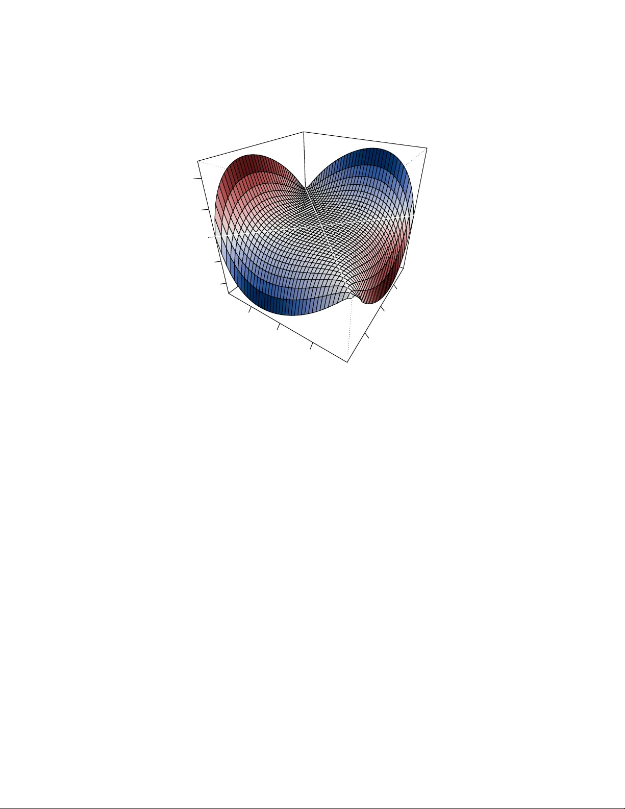
FIRST VERSUS FULL OR FIRST VERSUS LAST: U-ST A TISTIC CHANGE-POINT TESTS UNDER FIXED AND LOCAL AL TERNA TIVES HER OLD DEHLING, D ANIEL V OGEL, AND MAR TIN WENDLER Abstract. The use of U-statistics in the change-point con text has received considerable atten tion in the literature. W e compare tw o approac hes of constructing CUSUM-t ype c hange-p oin t tests, which w e call the first-vs-ful l and first-vs-last approac h. Both ha v e b een pursued b y differen t authors. The question naturally arises if the tw o tests substan tially differ and, if so, which of them is better in whic h data situation. In large samples, b oth tests are similar: they are asymptotically equiv alen t under the n ull hypothesis and under sequences of local alternativ es. In small samples, there may be quite noticeable differences, whic h is in line with a different asymptotic b ehavior under fixed alternatives. W e derive a simple criterion for deciding whic h test is more p ow erful. W e examine the examples Gini’s mean difference, the sample v ariance, and Kendall’s tau in detail. Particularly , when testing for changes in scale by Gini’s mean difference, we sho w that the first-vs- ful l approac h has a higher p ow er if and only if the scale changes from a smaller to a larger v alue – regardless of the p opulation distribution or the lo cation of the change. The asymptotic deriv ations are under weak dep endence. The results are illustrated by n umerical sim ulations and data examples. Contents 1. In tro duction 2 2. Asymptotic results 5 2.1. Null h yp othesis 5 2.2. Lo cal alternativ es 6 2.3. Fixed alternativ es 8 2.4. Consistency 10 2.5. Estimation of change lo cation 11 2.6. Asymptotic distribution under fixed alternativ es 11 3. Examples 12 3.1. Gini’s mean difference 12 3.2. The sample v ariance 15 3.3. Sample co v ariance 17 3.4. Kendall’s tau 17 4. Data example 19 5. Conclusion 21 Ac kno wledgments 23 Date : F ebruary 15, 2026. Key wor ds and phr ases. change-point analysis, CUSUM test, Gini’s mean difference, Kendall’s tau, sam- ple v ariance. MSC 2020: 62F03, 60F17, 62E20. 1 2 HEROLD DEHLING, D ANIEL VOGEL, AND MAR TIN WENDLER App endices 23 App endix A. A general, moment-free framework for dep enden t series 23 App endix B. Proofs of Section 2 and further results 24 B.1. Pro ofs of Section 2.1 (Null h yp othesis) 26 B.2. Pro ofs of Section 2.2 (Lo cal alternativ es) and further results 27 B.3. Conditions for Assumptions 2.5 to hold (Lo cal alternatives) 31 Indep enden t sequences 32 Dep enden t sequences 34 B.4. Pro ofs of Section 2.3 (Fixed alternativ es) 35 B.5. Conditions for Assumptions 2.8 to hold (Fixed alternativ es) 37 Indep enden t sequences 37 Dep enden t sequences 38 B.6. Pro ofs of Section 2.4 (Consistency) 38 B.7. Pro ofs of Section 2.5 (Estimation of change lo cation) 38 B.8. Pro ofs of Section 2.6 (Asymptotic distributions under fixed alternativ es) 40 App endix C. Proofs and further results for Section 3 49 App endix D. Details on long-run v ariance estimation 52 References 54 1. Introduction The classical approac h for testing the constancy of the mean of a time series X 1 , . . . , X n is the CUSUM test based on the test statistic (1.1) T n = max 1 ≤ k ≤ n k √ n   ¯ X 1: k − ¯ X 1: n   , where ¯ X i : j denotes the sample mean computed from X i , . . . , X j for an y t wo integers i, j suc h that 1 ≤ i < j ≤ n . The test statistic ma y equally b e written as (1.2) T n = max 1 ≤ k ≤ n k ( n − k ) n 3 / 2   ¯ X 1: k − ¯ X ( k +1): n   . These tw o represen tations (1.1) and (1.2) suggest tw o differen t views of the CUSUM test statistic: one ma y either view it, for eac h k , as a comparison of the sample mean of the first part of the sample X 1 , . . . , X k to the sample mean of the whole sample or as a comparison of the mean of the first part to the mean of the remaining part X k +1 , . . . , X n . When the CUSUM approac h is extended to a general setting, i.e., when we w an t to test the constancy of some parameter θ ∈ R of the marginal distribution of the observed pro cess, for which an estimator ˆ θ n is av ailable, we ma y consider either of the test statistics T 1 ( ˆ θ n ) = max 1 ≤ k ≤ n k n − 1 / 2 | ˆ θ 1: k − ˆ θ 1: n | and T 2 ( ˆ θ n ) = max 1 ≤ k ≤ n k ( n − k ) n − 3 / 2 | ˆ θ 1: k − ˆ θ ( k +1): n | with ˆ θ i : j b eing defined analogously to ¯ X i : j . If ˆ θ n is a line ar statistic, i.e., if (1.3) ˆ θ n = 1 n n X i =1 ξ ( X i ) U-ST A TISTIC CHANGE-POINT TESTS UNDER AL TERNA TIVES 3 for some function ξ , b oth test statistics are identical, but in general they are not. Both routes to generalizing the CUSUM test statistic, first-vs-ful l and first-vs-last , hav e b een tak en b y different authors. In the present pap er, we analyze the difference b etw een T 1 ( ˆ θ n ) and T 2 ( ˆ θ n ) in the case ˆ θ n is a U-statistic. Let ( X i ) i ∈ Z b e a p -dimensional, stationary sto chastic process. A one-sample U-statistic or order 2 is defined as (1.4) U n = 1  n 2  X 1 ≤ i 0. W e apply the studentized versions of the first-vs- ful l and the first-vs-last GMD test at the 5% significance level using the asymptotic null distribution and the v ariance estimator ˆ σ 2 GMD = 2 n n X i =1  1 n n X j =1 | X i − X j | − g n  2 , where g n is the sample GMD of X 1 , . . . , X n . W e observe the follo wing: (S1) F or sample size n = 4000 and σ = 1 . 08, the first-vs-ful l test has a p ow er of 0.79 and the first-vs-last test has a p ow er of 0.79. Their relative difference in p ow er is less than 0.1%. Under the null h yp otheses, i.e., σ = 1, b oth test hav e a rejection frequency of 0.05. (S2) F or sample size n = 60 and σ = 2 the first-vs-ful l test has a p ow er of 0.70 and the first-vs-last test has a p ow er of 0.61. If the v ariance changes from 1 to 0 . 5, the tw o tests hav e a p ow er of 0.65 and 0.71, resp ectively . In both cases, the relativ e difference is ab out 10%. Under the null h yp othesis, the size of b oth tests is b etw een 0.03 and 0.04. The rejection frequencies stated ab ov e are each based on 10,000 runs and rounded to t w o decimals. These n um b ers may serve as illustration for general principles which will b e sho wn in this pap er: (A) Both test statistics, T 1 ( h ) and T 2 ( h ), ha v e the same asymptotic distribution under the n ull hypothesis. (B) Both test statistics ha v e, for any non-degenerate U-statistic k ernel h , the same asymp- totic distribution under lo cal alternativ es. (C) F or sequences of fixed alternatives, the test statistics generally b ehav e differently . It do es dep end on the sp ecific alternativ e which test has a b etter p ow er. Particularly , the ranking of the tests is determined by only three n umbers: (1.6) θ F = E ( h ( X, X ′ )) , θ G = E ( h ( Y , Y ′ )) , and θ F G = E ( h ( X, Y ′ )) , where X , X ′ , Y , Y ′ are indep enden t with X , X ′ ∼ F , Y , Y ′ ∼ G and F and G b eing the data distributions b efore and after the change, resp ectively . (D) Sp ecifically for Gini’s mean difference, the first-vs-ful l test is alwa ys more p o werful if θ F < θ G , and it is less p o werful if θ F > θ G . (E) Sp ecifically for the sample v ariance, b oth tests are equally p ow erful unless there is a sim ultaneous change in mean. If there is a change in mean, the same relation as for Gini’s mean difference holds. P articularly , (B) implies that in large samples the tests ha v e a similar p o wer, whic h is illustrated by (S1) ab o ve. Lik ewise , (C) suggests that for smaller samples there may b e substan tial differences, as is illustrated by (S2). U-ST A TISTIC CHANGE-POINT TESTS UNDER AL TERNA TIVES 5 The organization of the pap er follows the outline ab ov e: In Section 2.1, we study b oth test statistics under the n ull hypothesis, in Section 2.2 under sequences of local alternatives. Section 2.3 is dev oted to fixed alternatives and the inv estigation of the differences of the tests. Within the fixed-alternative scenario, we further derive results ab out the consistency of the change-point tests (Section 2.4), the change-point lo cation estimation (Section 2.5), and the asymptotic normality of the test statistics (Section 2.6). In Section 3, we examine sev eral p opular U-statistics: Gini’s mean difference, the sample v ariance, the sample cov ari- ance, and Kendall’s tau. W e sho w in particular (D) and (E) and provide further sim ulation results. Section 4 contains data examples, Section 5 concludes. All pro ofs are deferred to the appendix in supplemen tary material. 2. Asymptotic resul ts W e study the asymptotic behavior of b oth test statistics under the n ull h yp othesis, under sequences of lo cal alternatives, under sequences of fixed alternativ es, and the asymptotic b eha vior of the corresp onding maximizing p oin ts, which serv e as estimators for the lo cation of the c hange under one-c hange-p oin t alternativ es. Throughout, ( X i ) i ∈ Z is a p -dimensional, strongly stationary sequence with marginal distribution F and h : R p × R p → R a symmetric k ernel function. W e restrict our attention to real-v alued kernels, but, as in the case of Kendall’s tau, the observ ations may b e multiv ariate. Define, for n ∈ N , the short-hand notation (2.1) D F n ( k ) = k ( U 1: k − U 1: n ) , 2 ≤ k ≤ n, and (2.2) D L n ( k ) = k ( n − k ) n  U 1: k − U ( k +1): n  , 2 ≤ k ≤ n, for the w eigh ted D ifferences processes of the first-vs- F ull and first-vs- L ast approac h, resp ec- tiv ely , so that the corresp onding test statistics (1.5) can b e written as T 1 ( h ) = n − 1 / 2 max 1 ≤ k ≤ n | D F n ( k ) | and T 2 ( h ) = n − 1 / 2 max 1 ≤ k ≤ n | D L n ( k ) | . 2.1. Null h yp othesis. The main to ol for treating U-statistics asymptotically is the Ho- effding decomposition. F or the stationary sequence ( X i ) i ∈ Z , w e write U 1: n as U 1: n = θ + 2 n n X i =1 h 1 ( X i ) + 2 n ( n − 1) X 1 ≤ i 0 (2.6)    p λ ( x )    +    ∂ ∂ λ p λ ( x )    ≤ v ( x ) for al l λ ∈ ( λ 0 − ϵ, λ 0 + ϵ ) and such that (2.7) Z Z | h ( x, y ) | v ( x ) v ( y ) dx dy < ∞ Then Assumption 2.4 is satisfie d for the distributions F and G n with densities f ( x ) and g n ( x ) as define d ab ove, and with ∆ = − 2 a Z Z h ( x, y ) ∂ ∂ λ p λ 0 ( x ) p λ 0 ( x ) dx. This co vers in particular the Gaussian scale family , whic h w e use extensiv ely in the sim ulations in Section 3, see Example B.3 in the App endix. Theorems 2.2 and 2.6 together state the t w o tests, the first-vs-ful l and the first-vs-last , are asymptotic al ly e quivalent , i.e., for an y array ( X in ) of random v ariables falling either under the n ull hypothesis or a lo cal alternativ e, the probabilit y of a differing test decision tends to zero as the sample size tends to infinity . 2.3. Fixed alternatives. So far we hav e noted that the tw o U-statistic c hange-p oin t test statistics are asymptotically equiv alen t. Nevertheless, noteworth y differences in p ow er are observ ed in simulations. The question remains if these differences can b e back ed b y theo- retical results and if conditions can b e given to identify situations where one test is b etter than the other. T ow ard this end, we consider sequences of fixed alternatives. Let ( X i ) i ∈ Z and ( Y i ) i ∈ Z b e t w o p -dimensional, strongly stationary sequences with marginal distribu- tions F and G , resp ectively . W e further require the 2 p -dimensional pro cess ( X i , Y i ) i ∈ Z to b e strongly stationary . Then the data array ( X in ) i ∈ Z ,n ∈ N is constructed analogously to the lo cal-alternativ e set-up: X in = ( X i for i ≤ [ nτ ⋆ ] , Y i for i ≥ [ nτ ⋆ ] + 1 U-ST A TISTIC CHANGE-POINT TESTS UNDER AL TERNA TIVES 9 for some fixed τ ⋆ ∈ (0 , 1). The observ ed data is, as b efore, the triangular cut-out ( X in ) 1 ≤ i ≤ n,n ∈ N . Let ( ˜ X in ) 1 ≤ i ≤ n,n ∈ N b e an indep endent copy of ( X in ) i ∈ Z ,n ∈ N . Recall the definitions of θ F , θ G , and θ F G , cf. (1.6), and let (2.8) ρ F G = θ F G − ( θ F + θ G ) / 2 . W e call ρ F G the e c c entricity of θ F G as it describ es the deviation of the mixed parameter θ F G from the midpoint b et ween θ F and θ G . This offset will play a crucial role in the follo wing: it determines the p ow er ranking of the test. Belo w we employ again the notation θ ij n , h 1 ij n ( x ), and h 2 ij n ( x, y ), as defined in (2.5), but k eep in mind that the arrays ( X in ) and ( ˜ X in ) are now defined slightly different than in Section 2.2. Assumption 2.8 . Let ( X in ) 1 ≤ i ≤ n,n ∈ N and h b e such that (1) the terms E  max l ≤ n    X 1 ≤ i θ G and θ G − θ F 2 < ρ F G < θ F − θ G 2( τ ⋆ − 1 + 1 /τ ⋆ ) , then | Ψ 1 ( t ) | < | Ψ 1 ( τ ⋆ ) | for al l t ∈ [0 , 1] with t  = τ ⋆ . The same is true if θ F < θ G and θ F − θ G 2( τ ⋆ − 1 + 1 /τ ⋆ ) < ρ F G < θ G − θ F 2 . (2) If θ F  = θ G and | ρ F G | ≤ 1 2 min { τ ⋆ 1 − τ ⋆ , 1 − τ ⋆ τ ⋆ }| θ F − θ G | , then for al l t ∈ [0 , 1] with t  = τ ⋆ | Ψ 2 ( t ) | < | Ψ 2 ( τ ⋆ ) | . Similar to the previous t w o results, the implications of Prop osition 2.12 are threefold: First, in a wide range of realistic application cases, b oth tests hav e the desired prop erty and b eha v e alike (consistency of the argmax lo cation estimator). Second, there is no general sup eriorit y of one test o ver the other: neither set of conditions in parts (1) and (2) of Propo- sition 2.12 implies the other. And lastly , the decisive criterion is again the e ccen tricit y ρ F G (it must not b e to o large in absolute v alue), and one can hence easily construct alternatives where the argmax estimator is consistent and alternatives where it is not, see Section 3.2 b elo w and Example C.2 in the supplementary material. 2.6. Asymptotic distribution under fixed alternatives. F rom Theorem 2.9 and Prop o- sition 2.12 we kno w that, under fixed alternativ es, the (1 / √ n )-scaled test statistics n − 1 / 2 T 1 ( h ) and n − 1 / 2 T 2 ( h ) conv erge in probabilit y to differen t v alues Ψ 1 ( τ ⋆ ) and Ψ 2 ( τ ⋆ ), resp ectively . T o complete the asymptotic analysis of the first-vs-ful l and the first-vs-last approach, w e study the asymptotic distribution of the t wo test statistics within the fixed-alternative set- up. W e demonstrate that they differ not only in mean, but we also obtain asymptotic 12 HEROLD DEHLING, DANIEL VOGEL, AND MAR TIN WENDLER v ariances that are generally different. This b ecomes apparent for univ ariate and indep en- den t data sequences and w e restrict our deriv ations to this scenario in the follo wing. Using the notation introduced at the b eginning of Section 2.3 define further h F ( x ) = Z h ( x, y ) dF ( y ) , h G ( x ) = Z h ( x, y ) dG ( y ) . Theorem 2.13. L et the triangular arr ay ( X in ) 1 ≤ i ≤ n,n ∈ N b e r ow-w ise indep endent, and let the assumptions of The or em 2.9 and Pr op osition 2.12 b e satisfie d. L et further the kernel h : R 2 → R b e such that θ F  = θ G and the inte gr als Z Z h 2 ( x, y ) dF ( x ) dF ( Y ) , Z Z h 2 ( x, y ) dF ( x ) dG ( Y ) , Z Z h 2 ( x, y ) dG ( x ) dG ( Y ) ar e al l finite. Then  T 1 ( h ) − √ n | Ψ 1 ( τ ⋆ ) |  → Z 1 ,  T 2 ( h ) − √ n | Ψ 2 ( τ ⋆ ) |  → Z 2 in distribution as n → ∞ , wher e Z 1 , Z 2 ar e c enter e d normal r andom variables with varianc es V ar[ Z 1 ] = 4 τ ⋆ V ar[ h F ( X ) − τ ⋆ h G ( X )] + 4 τ ⋆ 2 (1 − τ ⋆ )V ar[ h G ( Y )] , V ar[ Z 2 ] = 4 τ ⋆ (1 − τ ⋆ ) 2 V ar[ h F ( X )] + 4 τ ⋆ 2 (1 − τ ⋆ )V ar[ h G ( Y )] for a r andom variable X with distribution function F and a r andom variable Y with distri- bution function G . If w e hav e a strictly linear U-statistic, i.e., h ( x, y ) = 1 2 ( h ( x, x ) + h ( y , y )), b oth test statistics are equal, and should hav e the same limit v ariance. This is indeed the case: In this situation, h F ( x ) = 1 2 h ( x, x ) − E [ 1 2 h ( X , X )] and h G ( x ) = 1 2 h ( x, x ) − E [ 1 2 h ( Y , Y )], so V ar[ h F ( X ) − τ ⋆ h G ( X )] = V ar[(1 − τ ⋆ ) h F ( X )] = (1 − τ ⋆ ) 2 V ar[ h F ( X )] and consequently V ar[ Z 1 ] = V ar[ Z 2 ]. This argument do es not apply if the U-statistic is not linear, and the asymptotic v ariances are generally differen t. 3. Examples W e examine four well-kno wn U-statistics in detail: Gini’s mean difference, the sample v ariance, the sample cov ariance, and Kendall’s tau. The former t w o can b e used to detect c hanges in the scale of univ ariate series. So in Sections 3.1 and 3.2 we assume the data series to b e univ ariate with distributions F and G b efore and after the p oten tial c hange-p oin t. In case F and G p ossess Leb esgue densities f and g , resp ectively , w e hav e the following represen tation of the eccen tricit y ρ F G , whic h will b e emplo yed in Prop osition 3.1. (3.1) ρ F G = − 1 2 Z Z h ( x, y ) { f ( x ) − g ( x ) }{ f ( y ) − g ( y ) } dxdy . 3.1. Gini’s mean difference. W e consider the kernel h ( x, y ) = | x − y | , leading to Gini’s mean difference U 1: n = 2 n ( n − 1) X 1 ≤ i 0, a quic k calculation yields θ F = 2 √ π , θ G = 2 √ π σ, θ F G = 2 √ π r 1 2 (1 + σ 2 ) and hence ρ F G = θ F G − ( θ F + θ G ) / 2 ≥ 0. W e find the eccen tricit y is alwa ys p ositive for σ  = 1. This holds indeed generally . Prop osition 3.1. L et the univariate distributions F and G with L eb esgue densities f and g , r esp e ctively, have finite first moments. Then, for the kernel h ( x, y ) = | x − y | , we have ρ F G ≥ 0 . Consequen tly , the p ow er ranking of b oth change-point tests is solely determined by the order of θ F and θ G . F ollowing our criterion from Section 2.3, the first-vs-ful l test is more p o w erful than the first-vs-last test if θ G − θ F > 0, i.e., if the scale of the series changes from a smaller v alue to a larger one. The first-vs-ful l is less p ow erful than the first-vs-last if the scale decreases after the c hange. This is regardless of where the change occurs and of any other aspect of F and G suc h as, e.g., a simultaneous change in lo cation. Also, w e find in the normal examples that θ F G is alwa ys b etw een θ F and θ G . This is also generally true for median-centered sequences. Prop osition 3.2. L et h ( x, y ) = | x − y | and X ∼ F with E | X | < ∞ and F (0) = 1 / 2 , i.e, X is me dian-c enter e d. F urthermor e, for c > 0 , we denote by G = G c the distribution function of cX . Then θ F G ∈ [min { θ F , θ G } , max { θ F , θ G } ] Visualization. Figure 1 illustrates Theorem 2.9 for Gini’s mean difference. The set-up is similar to the simulation example in the Introduction. W e consider a series of indep endent observ ations stemming from F = N (0 , 1) b efore the change at τ ⋆ = 1 / 3 and G = N (0 , 4) afterw ards. The dashed lines in b oth panels depict the limit functions Ψ 1 ( first-vs-ful l test; dark blue) and Ψ 2 ( first-vs-last test; ligh t blue). The jagged lines sho w tra jectories of the corresp onding pro cesses  1 n D F n ( k )  1 ≤ k ≤ n and  1 n D L n ( k )  1 ≤ k ≤ n based on a sequence of n indep enden t observ ations with n = 100 (left panel) and n = 4000 (right panel). Figure 1 visualizes the con verges of the processes to their resp ectiv e deterministic limit as stated by Theorem 2.9. The difference b etw een the tra jectories can b e seen to b e essen tially captured b y the difference b etw een the resp ectiv e limit processes. Sim ulation results. W e consider indep enden t Gaussian pro cesses only . The sample sizes are n = 63 , 250 , 1000 , 4000 with p oten tial c hange-point lo cations at τ ⋆ = 1 / 4 , 1 / 2 and 3 / 4. The heigh t of the c hange is sample-size dep endent. The three scenarios are as follo ws: (1) Null hypothesis: No change o ccurs. The data are standard normal iid sequences. (2) Alternative 1: Before the c hange-p oin t, the observ ations hav e standard deviation 1 and after the change σ n = 1 + 3 / √ n , e.g., σ 63 ≈ 1 . 378, σ 4000 ≈ 1 . 047. (3) Alternative 2: Before the change-point, the observ ations hav e standard deviation σ n and afterw ards 1. T able 1 sho ws empirical rejection frequencies of the first-vs-ful l test and the first-vs-last test for Gini’s mean difference at the asymptotic 5% level. Both test statistics are divided 14 HEROLD DEHLING, DANIEL VOGEL, AND MAR TIN WENDLER 0.0 0.2 0.4 0.6 0.8 1.0 −0.30 −0.25 −0.20 −0.15 −0.10 −0.05 0.00 n = 100 first vs full first vs last 0.0 0.2 0.4 0.6 0.8 1.0 −0.30 −0.25 −0.20 −0.15 −0.10 −0.05 0.00 n = 4000 Ψ 1 Ψ 2 Figure 1. Visualization of Theorem 2.9 for Gini’s mean difference: A c hange o ccurs at τ ⋆ = 1 / 3 from F = N (0 , 1) to G = N (0 , 4). The limit functions Ψ 1 ( first-vs-ful l test; dark blue) and Ψ 2 ( first-vs-last test; ligh t blue) as giv en in Theorem 2.9 along with corresp onding tra jectories of  1 n D F n ( k )  1 ≤ k ≤ n and  1 n D L n ( k )  1 ≤ k ≤ n for a sequence of n indep endent obser- v ations with n = 100 (left panel) and n = 4000 (righ t panel). b y the square ro ot of a long-run v ariance estimate using the Bartlett kernel and a sample- size-dep enden t bandwidth b n = n 1 / 3 , see App endix D. The th us obtained studen tized test statistics are compared to the 95% quantile of the Kolmogoro v distribution, see Remark 2.3 (2). W e observ e the follo wing: As exp ected, a change in the middle of the data ( τ ⋆ = 1 / 2) is easier to detect than an early or late change. Although the height of the c hange was adjusted for the sample size, we see an increase in p ow er with growing sample size n . Concerning the comparison of the tw o approaches, we find our exp ectations based on the theoretical results confirmed: The first-vs-ful l test has a higher p ow er when the v ariance is increasing (Alternativ e 1), while the first-vs-last v ersion has higher p o wer for a decreasing v ariance (Alternativ e 2). The p o wer ranking is indep endent of the lo cation of τ ⋆ . The difference in p ow er is most pronounced for the smallest sample size n = 63. F or n = 4000, the p o w er difference is very small, which is not surprising, as the tw o tests are asymptotically equiv alen t (Theorem 2.6). An asp ect not pursued in this pap er is why one would use Gini’s mean difference as scale estimator in the first place. There are go o d reasons to do so: The estimator Gini’s me an difference is – for practical purp oses – as efficient as the standard deviation at the normal mo del (Nair, 1936), which w e find reflected in the p ow ers of the corresp onding tests when comparing T able 1 to T able 2. F urthermore, Gini’s mean difference is more efficient than the U-ST A TISTIC CHANGE-POINT TESTS UNDER AL TERNA TIVES 15 T able 1. Gini’s mean difference. Empirical rejection frequencies (%) at the 5% significance level of the first-vs-ful l (FvsF) and first-vs-last (FvsL) c hange-p oin t test. Studentized with long-run v ariance estimation (bandwidth b n = n 1 / 3 ). 2000 runs. Sample size n Scenario c hange lo cation test statistic 63 250 1000 4000 Null h yp othesis FvsF 2.9 3.6 4.0 3.8 FvsL 2.1 3.3 4.0 3.9 Alternativ e 1 0.25 FvsF 15.8 28.9 36.8 43.6 0.25 FvsL 9.2 25.1 35.2 42.6 0.5 FvsF 39.5 55.8 63.2 68.8 0.5 FvsL 25.8 51.7 61.5 68.0 0.75 FvsF 26.0 36.5 41.8 43.7 0.75 FvsL 12.7 29.0 39.2 42.1 Alternativ e 2 0.25 FvsF 5.9 25.8 38.1 43.7 0.25 FvsL 9.5 28.6 39.6 44.5 0.5 FvsF 16.8 46.9 60.8 69.8 0.5 FvsL 28.7 51.5 63.1 70.3 0.75 FvsF 4.0 19.6 33.5 41.8 0.75 FvsL 10.8 26.2 36.2 43.7 standard deviation at heavier-tailed distributions (Gerstenberger and V ogel, 2015), which translates to b etter p o wers of the resp ectiv e c hange-p oin t tests (Gerstenberger et al., 2020). 3.2. The sample v ariance. The sample v ariance is obtained by the kernel h ( x, y ) = ( x − y ) 2 / 2, leading to the U-statistic U 1: n = 1 n ( n − 1) X 1 ≤ i θ G , the first-vs-last test is more p ow erful. This holds regardless of the direction of the c hange in mean or where the c hange o ccurs. By Corollary 2.11, w e ha v e that, as long as there is a c hange in v ariance, b oth tests are consisten t. Corollary 2.11 tells further that, if there is no change in v ariance, a c hange in mean renders b oth tests consistent as well. The same holds true for Gini’s mean difference, see Example C.1. F urthermore, by Prop osition 2.12, one can easily construct fixed alternatives where b oth argmax change lo cation estimators are consisten t and fixed alternatives where b oth are not consisten t, simply b y making the difference of the means sufficiently small or large compared to the difference of the v ariances. Incidentally , this is also similarly true for Gini’s mean difference, see Example C.2. Last but not least, one can use Prop osition 3.3 to construct in teresting sequences of lo c al alternativ es. F or instance, consider the sequence of local alternatives F = N (0 , 1) and G n = N ( n − 1 / 4 µ, 1 + n − 1 / 2 ∆) for any real num b ers µ, ∆  = 0. This sequence satisfies Assumption 2.4 (1), i.e., θ F and θ G approac h each other at the 1 / √ n rate, but not Assumption 2.4 (2). The pro cesses ( n − 1 / 2 D F n ([ nt ])) 0 ≤ t ≤ 1 and ( n − 1 / 2 D L n ([ nt ])) 0 ≤ t ≤ 1 con v erge to different limit pro cesses in this case, which can b e seen from the proof of Theorem 2.6, and hence b oth tests hav e different asymptotic pow er. Sim ulation results. W e consider the exact same set-up as in Section 3.1. Again, we apply studen tization with a long-run v ariance estimate using the Bartlett kernel and the band- width b n = n 1 / 3 . The results are given in T able 2. F or n = 250 and larger, the p ow er of b oth tests is essentially the same. F or n = 63, there are some noticeable differences. Except for τ ⋆ = 0 . 75 under Alternative 1, the difference stays within a 2%-p oints margin. It should b e noted that the differences for n = 63 are less pronounced if a smaller bandwidth in the long-run v ariances estimation is used. U-ST A TISTIC CHANGE-POINT TESTS UNDER AL TERNA TIVES 17 T able 2. Sample V ariance. Empirical rejection frequencies (%) at the 5% sig- nificance level of the first-vs-ful l (FvsF) and first-vs-last (FvsL) change-point test. Studen tized with long-run v ariance estimation (bandwidth b n = n 1 / 3 ). 2000 runs. Sample size n Scenario c hange lo cation τ ⋆ test statistic 63 250 1000 4000 Null h yp othesis FvsF 2.9 3.2 4.3 4.4 FvsL 3.3 3.2 4.3 4.4 Alternativ e 1 0.25 FvsF 6.0 18.6 33.8 42.0 0.25 FvsL 6.4 18.3 33.9 41.8 0.5 FvsF 24.5 50.6 63.9 68.7 0.5 FvsL 26.0 50.5 63.6 68.6 0.75 FvsF 17.6 35.4 43.2 45.6 0.75 FvsL 22.1 35.9 43.4 45.6 Alternativ e 2 0.25 FvsF 22.5 34.4 42.4 45.8 0.25 FvsL 20.4 34.1 42.4 45.8 0.5 FvsF 28.7 51.3 63.5 68.2 0.5 FvsL 26.7 51.2 63.4 68.2 0.75 FvsF 8.6 20.1 33.1 40.5 0.75 FvsL 7.6 20.0 33.1 40.6 3.3. Sample cov ariance. The sample co v ariance U 1: n = 1 n ( n − 1) X 1 ≤ i 0 } − 1 { ( x 2 − x 1 )( y 2 − y 1 ) < 0 } . Con trary to Gini’s mean difference and the sample v ariance, for this k ernel h , the eccentricit y ρ F G ma y b e p ositiv e, zero, or negativ e. The ranking of the tests is not solely determined by 18 HEROLD DEHLING, DANIEL VOGEL, AND MAR TIN WENDLER rho1 −0.5 0.0 0.5 rho2 −0.5 0.0 0.5 eccentricity rho_FG −0.04 −0.02 0.00 0.02 0.04 Figure 2. The plot of Example 3.5: It shows the eccentricit y ρ F G on the z-axis as a function of ρ 1 and ρ 2 , i.e., the correlation of the biv ariate centered Gaussian time series b efore and after the change, resp ectively . In the blue region, the first-vs-ful l test is more efficient. the sign of θ G − θ F . The next prop osition states that under certain symmetry conditions on F and G , the eccentricit y is zero. Prop osition 3.4. L et ( X , Y ) ∼ F and G b e such that ( X , − Y ) ∼ G , then, for the kernel h given by (3.2), we have ρ F G = 0 . Example 3.5 (Biv ariate normal distribution) . Consider the biv ariate distribution functions F and G with F = N 2  0 0  ,  1 ρ 1 ρ 1 1  and G = N 2  0 0  ,  1 ρ 2 ρ 2 1  for correlation parameters − 1 < ρ 1 , ρ 2 < 1. The corresp onding v alues of Kendall’s tau are θ F = (2 /π ) arcsin( ρ 1 ) and θ G = (2 /π ) arcsin( ρ 2 ). Figure 2 depicts the eccentricit y ρ F G as function of ρ 1 and ρ 2 and was created by means of numerical integration. The surface is shaded in blue where the first-vs-ful l test is b etter, i.e., where ρ F G has the same sign as θ G − θ F . It is shaded in red where first-vs-last is b etter. On the diagonals, i.e., for ρ 1 = ρ 2 (no c hange) and ρ 1 = − ρ 2 (the situation of Prop osition 3.4), the eccentricit y is zero. Sim ulation results. T able 3 con tains rejection frequencies of the studentized first-vs-ful l and the first-vs-last change-point tests for Kendall’s tau at the asymptotic 5% significance lev el based on 2000 runs for each case. The long-run v ariance estimator uses a Bartlett kernel U-ST A TISTIC CHANGE-POINT TESTS UNDER AL TERNA TIVES 19 T able 3. Kendall’s τ . Empirical rejection frequencies (%) at the 5% significance lev el of the first-vs-ful l (FvsF) and first-vs-last (FvsL) c hange-p oin t test. 2000 runs. With long-run v ariance estimation (bandwidth b n = n 1 / 3 ). c hange test sample size n scenario lo cation τ ⋆ statistic 63 250 1000 4000 NH FvsF 5.3 4.0 4.4 4.8 ρ 1 = ρ 2 = − 3 / √ n FvsL 3.8 4.0 4.0 4.8 Alternativ e 1 0.5 FvsF 55.2 68.0 71.9 73.4 ρ 1 = − 3 / √ n , ρ 2 = 3 / √ n FvsL 53.8 67.6 71.9 73.7 Alternativ e 2 0.5 FvsF 62.1 68.2 72.2 72.9 ρ 1 = 0, ρ 2 = 6 / √ n FvsL 70.1 69.2 71.5 73.2 Alternativ e 3 0.5 FvsF 76.6 70.8 71.0 71.7 ρ 1 = − 6 / √ n , ρ 2 = 0 FvsL 69.7 69.4 71.4 71.6 and bandwidth b n = n 1 / 3 , and is explicitly stated in App endix D. The data sequence are indep enden t biv ariate normal v ariates as in Example 3.5. F our scenarios are considered: (1) Null hypothesis: ρ 1 = ρ 2 = − 3 / √ n , (2) Alternative 1: ρ 1 = − 3 / √ n , ρ 2 = 3 / √ n , (3) Alternative 2: ρ 1 = 0, ρ 2 = 6 / √ n , (4) Alternative 3: ρ 1 = − 6 / √ n , ρ 2 = 0. The change alwa ys o ccurs in the middle of the series at τ ⋆ = 1 / 2. With the sample-size dep enden t c hange heigh t, w e mimic the lo cal-alternative setting, and obtain non-trivial p o w ers for all sample sizes. W e find: Both tests keep the nominal 5% level for sample sizes of at least n = 250. F or large n and changes of small magnitude, b oth tests hav e similar p ow er. F or n = 4000, all rejection frequencies are within a 0.5%-p oint margin of eac h other. This is in line with Theorem 2.6. F or small n and large changes, we observe substan tial differences in p o w er, which are in line with Theorem 2.9 and its consequences: Under all three alternatives, w e ha v e θ G − θ F > 0. By Example 3.5 we know that, under Alternativ e 2, the eccentricit y ρ F G is negative, and hence by the criterion from Section 2.3 the first-vs-last test is more p ow erful. Indeed, for n = 63, w e observ e an 8%-p oints higher p o w er of the first-vs-last test. Under Alternative 3, the picture is reversed: The eccentricit y is p ositive, has the same sign as θ G − θ F . Accordingly , we find the first-vs-ful l test to b e more p ow erful by the same magnitude. Under Alternativ e 1, b oth tests ha v e similar p ow er with a difference of ab out 1.5%-p oints for n = 63 and less for higher sample sizes. This illustrates Proposition 3.4. 4. D a t a example Figure 3 sho ws the ann ual mean discharge ( m 3 /s ) of the Colorado riv er at Lees F erry , AZ, and Cameo, CO, in the 88 years from 1934 to 2021. The data are taken from the webpages 20 HEROLD DEHLING, DANIEL VOGEL, AND MAR TIN WENDLER 0 5000 10000 15000 20000 25000 1935 1945 1955 1965 1975 1985 1995 2005 2015 m 3 s Lees Ferry , AZ Cameo, CO Figure 3. Annual mean discharge ( m 3 /s ) of the Colorado riv er at Lees F erry , AZ (darkblue) and Cameo, CO (ligh tblue) from 1934 to 2021. −1.5 −1.0 −0.5 0.0 0.5 1.0 1.5 1935 1945 1955 1965 1975 1985 1995 2005 2015 first vs full (p−v alue: 0.076) first vs last (p−v alue: 0.019) 5% significance threshold Figure 4. Gini’s mean difference: studen tized change-point pro cesses first- vs-ful l and first-vs-last applied to the Lees F erry series. of the U.S. Geological Service. 1 Lees F erry , AZ, is downstream from Glen Can y on Dam, whic h w as built from 1956 to 1964 and creates Lak e P o w ell. The resulting structural c hange in the ann ual mean disc harge series is clearly visible, affecting particularly the v ariabilit y of the series. Incidentally , the south w estern North American megadrought in recen t years (e.g. Overpeck and Udall, 2020; Williams et al., 2022) do es not b ecome apparent at the series: The disc harge downstream from Lak e Po well remained largely constant (while its w ater level has b een dramatically decreasing). Figure 4 shows the studentized change-point pro cesses first-vs-ful l and first-vs-last , cf. (2.1) and (2.2), for Gini’s mean difference applied to the Lees F erry sequence. All tests in this section use a long-run v ariance estimate with Bartlett kernel and bandwidth b = 2, see App endix D in the supplemen tary material for details. F rom the results of Section 3.1 we 1 h ttps://w aterdata.usgs.go v/nwi s U-ST A TISTIC CHANGE-POINT TESTS UNDER AL TERNA TIVES 21 −1.5 −1.0 −0.5 0.0 0.5 1.0 1.5 1935 1945 1955 1965 1975 1985 1995 2005 2015 first vs full (p−v alue: 0.164) first vs last (p−v alue: 0.184) 5% significance threshold Figure 5. Gini’s mean difference: studen tized change-point pro cesses first- vs-ful l and first-vs-last applied to the Cameo series. kno w that under alternatives where the scale de cr e ases , as it is the case here, the first-vs- last change-point test is more p o werful than the first-vs-ful l test. Indeed, the first-vs-last c hange-p oin t pro cess deviates further from zero, clearly exceeding the asymptotic 5% sig- nificance threshold of ± 1 . 3581, yielding a p-v alue of 0.019. The first-vs-ful l change-point pro cess narrowly stays within the 5% threshold, and the test returns a mild ly signific ant p-v alue of 0.076. Cameo, CO, is lo cated upstream from Lake Po well and is not affected b y any ma jor h ydrological constructions. A pronounced change in scale is neither visible nor plausible for this series. Both Gini’s-mean-difference change-point pro cesses, first-vs-ful l and first- vs-last , are very close to each other, returning p-v alues of 0.164 and 0.184, respectively , cf. Figure 5. Another exp ectable consequence of the construction of the dam is a low er correlation b et w een discharges upstream and downstream from the reserv oir. Figure 6 shows b oth c hange-p oin t pro cesses for Kendall’s tau rank correlation co efficient b etw een the tw o dis- c harge series. In this case, the first-vs-ful l pro cess deviates further than the first-vs-last . The former yields a p-v alue of 0.006, the latter of 0.02. This fits in with the observ ations of Section 3.4, where w e noted that – at least for the normal mo del – the first-vs-ful l Kendall’s- tau test is more p ow erful than first-vs-last under alternativ es where the absolute value of the correlation co efficient decreases. Here, Kendall’s tau essentially decreases from 0.77 in the p eriod 1934–1962 to 0.43 in the p erio d 1965–2021. So here we find a similar picture as in Figure 4 with roles of the t w o tests interc hanged. 5. Conclusion W e studied tw o construction principles of generalized CUSUM test statistics: F or e ac h p oten tial change-point k , the first-vs-ful l approac h compares the estimate ˆ θ 1: k ev aluated at the first k observ ations to the estimate ˆ θ 1: n ev aluated at the whole sample, whereas the first-vs-last approach compares ˆ θ 1: k to the estimate ˆ θ ( k +1): n ev aluated at the remaining n − k observ ations. 22 HEROLD DEHLING, DANIEL VOGEL, AND MAR TIN WENDLER −1.5 −1.0 −0.5 0.0 0.5 1.0 1.5 1935 1945 1955 1965 1975 1985 1995 2005 2015 first vs full (p−v alue: 0.006) first vs last (p−v alue: 0.02) 5% significance threshold Figure 6. Kendall’s τ b etw een Lees F erry and Cameo: studentized c hange- p oin t processes first-vs-ful l and first-vs-last . Within the huge b o dy of literature devoted the change-point problem, authors usually consider one the of tw o approac hes without an y men tion of the respective other or a motiv a- tion of their choice. An exception is Sen (1983), who remarks that they are asymptotically equiv alen t. When discussing the question with colleagues, w e encoun tered tw o opinion camps: Either it is assumed that b oth approaches are generally very similar (as they are iden tical for the original CUSUM test with the sample mean) or it is exp ected that the first-vs-last is generally more p o werful. In this pap er, w e giv e a thorough comparison of the tw o approaches for the class of U-statistics. It turns out that the answer is not as unanimous as rep eatedly b eliev ed: First, the tw o test approaches hav e common prop erties: Under the null hypothesis and lo cal alternatives, where the change-point pro cesses ( D F n ([ nt ])) 0 ≤ t ≤ 1 and ( D L n ([ nt ])) 0 ≤ t ≤ 1 are scaled with 1 / √ n , they hav e the same limit. This can b e summarized by sa ying, they are asymptotically equiv alent. Ho w ever, when scaling with 1 /n in the fixed-alternativ es setting, different limits app ear, whic h is reflected by p ow er differences in small to mo derate sample sizes. W e identify a simple criterion to determine which test is more p ow erful in which situation: the sign of the eccentricit y ρ F G relativ e to the sign of θ G − θ F . The eccentricit y ρ F G of the kernel h at distributions F and G describ es the offset of the mixed parameter θ F G from the cen ter of the interv al b etw een θ F and θ G . Consequently , since the eccen tricit y is symmetric in F and G , w e ha v e that, for an y alternative where first-vs-ful l is more p ow erful, an equally relev an t alternativ e can b e giv en where first-vs-last is more p ow erful by the same order of magnitude – by simply exc hanging F and G . The ensuing question for future researc h is if similar criteria can be giv en for other classes of statistics, e.g., quantile-based estimators (e.g. median, interquartile range), rank-based statistics (e.g. Sp earman’s rho), or the large class of differen tiable functionals of statistics. U-ST A TISTIC CHANGE-POINT TESTS UNDER AL TERNA TIVES 23 A ckno wledgments W e thank Svenja Fischer for p oin ting us to the data source. All figures and simulations w ere done in R 4.1.3 (R Core T eam, 2022) using pac k ages m vtnorm (Genz and Bretz, 2009), p caPP (Filzmoser et al., 2022), and cubature (Narasimhan et al., 2022). Appendices There are in total four app endices: App endix A presen ts the concept of near ep o ch dep endence in probabilit y ( P -NED), where w e essentially follo w Dehling et al. (2017). This class of weakly dep endent pro cesses extends the L 2 -NED class to essentially arbitrarily hea vy-tailed marginal distributions. Within this framew ork w e state regularit y assumptions on the data pro cess and on the U-statistics that guaran tee the high-level conditions we imp ose in the theorems throughout the pap er. Appendix B con tains the pro ofs of the results of Section 2. App endix C contains pro ofs of Section 3. App endix D explicitly states the long-run v ariance estimators used in the sim ulations and the data examples. Appendix A. A general, moment-free framework for dependent series Definition A.1 (Absolute regularit y) . Let (Ω , F , P ) b e a probability space. (1) F or tw o sub- σ -fields A , B of F , w e define the absolute regularity co efficient β ( A , B ) = E [ess sup {| P ( A |B ) − P ( A ) | : A ∈ A} ] . The absolute regularity co efficien t is a measure of dep endence b et w een the σ -fields A and B , it lies betw een 0 and 1, and equals 0 if A and B are indep endent. (2) Let ( Z n ) n ∈ Z b e an r -v ariate, strongly stationary sto c hastic pro cesses on (Ω , F , P ). F or k ≤ n , let F n k = σ ( Z k , . . . , Z n ), where also k = −∞ and n = ∞ are p ermitted. The pro cess ( Z n ) n ∈ Z is called absolutely r e gular if the absolute regularity co efficients β k = β ( F 0 −∞ , F ∞ k ) , k ≥ 1 , con v erge to zero as k → ∞ . Absolute regularit y is also referred to as β -mixing and goes back to V olkonskii and Rozano v (1959). It is a mixing condition stronger than α -mixing and w eak er than ϕ -mixing. Ho w ever, we do not consider absolutely regular pro cesses themselves, but appro ximating functionals of such absolutely regular pro cesses. Sp ecifically , w e use the concept of near ep o ch dep endence in probabilit y ( P -NED). It w as introduced by Dehling et al. (2017) and generalizes the L 2 -NED concept. It is as general as L 2 -NED concerning the serial dep en- dence, but imp oses no momen t conditions. This is useful for b ounded U-statistics lik e Kendall’s tau. Their asymptotics are v alid without any momen t assumptions, and P -NED pro vides a framework for w eakly dep enden t and v ery heavy-tailed sequences. Definition A.2 . Let ( Z in ) i ∈ Z ,n ∈ N b e an array of r -v ariate sto c hastic pro cesses ( n denoting the ro w index). The arra y ( X in ) i ∈ Z ,n ∈ N of p -v ariate sto chastic processes is called ne ar ep o ch dep endent in pr ob ability or short P -ne ar ep o ch dep endent ( P -NED) on the arra y ( Z in ) n ∈ Z if there is a sequence of approximating constants ( a k ) k ∈ N with a k → 0 as k → ∞ , functions 24 HEROLD DEHLING, DANIEL VOGEL, AND MAR TIN WENDLER f n,i,k : R r × (2 k +1) → R p , k ∈ N , and a non-increasing function Φ : (0 , ∞ ) → (0 , ∞ ) such that (A.1) P  | X in − f n,i,k ( Z i − k,n , . . . , Z i + k,n ) | 1 > ε  ≤ a k Φ( ε ) for all k , n ∈ N , i ∈ Z and ε > 0. Here | x | 1 denotes the L 1 -norm of the vector x ∈ R p . F or the most part of Section 2 of the pap er we consider triangular arrays of pro cesses. Hence we define P -NED for arrays, noting that this includes P -NED sequences as sp ecial case b y simply taking all rows identical. F or the v arious functional limit theorems for the pro cesses D F n and D L n , cf. (2.1) and (2.2), resp ectiv ely , in the main pap er, we require the following technical Assumptions A.3, A.4, and A.5 on the data array ( X in ) i ∈ Z ,n ∈ N and the kernel h . Assumption A.3 (W eak dep endence) . The array ( X in ) i ∈ Z ,n ∈ N is P -NED on an absolutely regular arra y ( Z in ) i ∈ Z ,n ∈ N , and there is a δ > 0 such that a k Φ( k − 6 ) = O ( k − 6(2+ δ ) /δ ) , ∞ X k =1 k β δ / (2+ δ ) k < ∞ , where β k , k ∈ N are the absolute regularit y co efficients (Definition A.1) and a k , k ∈ N , and Φ are as in Definition A.2. F urthermore, a uniform moment condition on h ( X i , X j ) is required. W e do not imp ose an y moment conditions on the data sequence itself. Assumption A.4 (Uniform momen ts) . There is a constan t M > 0 such that for all k , n ∈ N and i, j ∈ { 1 , . . . , n } E | h ( X in , X j n ) | 2+ δ ≤ M , E | h ( f n,i,k ( Z i − k,n , . . . , Z i + k,n ) , f n,j,k ( Z j − k ,n , . . . , Z j + k ,n )) | 2+ δ ≤ M . Assumptions A.3 and A.4 are link ed via δ . W eak er moment conditions hav e to b e paid for by a faster decay of the short-range dep endence co efficients and vice versa. The last assumption is also known as the v ariation condition and was introduced b y Denker and Keller (1986). It is a form of Lipschitz contin uit y of the kernel h with resp ect to F . Assumption A.5 (V ariation condition) . Let ( ˜ X in ) i ∈ Z ,n ∈ N b e an indep endent copy of the arra y ( X in ) i ∈ Z ,n ∈ N . There are constan ts L, ϵ 0 > 0 such that for all ϵ ∈ (0 , ϵ 0 ), all n ∈ N , i, j ∈ { 1 , . . . , n } E sup | x − X in |≤ ϵ, | y − ˜ X j n |≤ ϵ    h ( x, y ) − h  X in , ˜ X j n     ! 2 ≤ Lϵ. Appendix B. Proofs of Section 2 and fur ther resul ts Prop osition B.1 b elow will b e emplo y ed in b oth Subsections B.1 Pr o ofs of Se ction 2.1 (Nul l hyp othesis) and B.2 Pr o ofs of Se ction 2.2 (L o c al alternatives) and further r esults . It is form ulated in terms of the arra y ( X in ) i ∈ Z ,n ∈ N as constructed at the b eginning of Section 2.2 (Lo cal alternatives) in the main pap er. When applying it to the null-h yp othesis case, it is understo o d that the arra y consists of identical ro ws ( X i ) i ∈ Z . As in the main pap er, U-ST A TISTIC CHANGE-POINT TESTS UNDER AL TERNA TIVES 25 w e henceforth usually omit the commas separating sev eral indices as long as there is no am biguit y . Let ( ˜ X in ) i ∈ Z ,n ∈ N b e an indep enden t cop y of ( X in ) i ∈ Z ,n ∈ N and define θ ij n = E h h ( X in , ˜ X j n ) i , h 1 ij n ( x ) = E [ h ( x, X j n )] − θ ij n , (B.1) h 2 ij n ( x, y ) = h ( x, y ) − E [ h ( X in , y )] − E [ h ( x, X j n )] + θ ij n . This is the same as (2.5) in the main pap er. Define further U (2) n, 1 ( l ) = 2 l ( l − 1) X 1 ≤ i λ 0 suc h that E  | h ( X , Y ) | ( X 2 + 1)( Y 2 + 1)  < ∞ , where X, Y are t w o indep endent N (0 , b 2 )-distributed random v ariables. B.3. Conditions for Assumptions 2.5 to hold (Lo cal alternatives). In this section w e giv e sp ecific conditions on the array ( X in ) i ∈ Z ,n ∈ N and the U-statistic k ernel h whic h ensure that Assumption 2.5 is satisfied. W e do so for tw o situation: for indep enden t observ ations and within the P -NED framew ork of Section A for dep endent observ ations. W e first state a technical lemma whic h is used in b oth situations. Recall the construction of the “lo cal-alternative array” ( X in ) i ∈ Z ,n ∈ N from the stationary pro cess ( X i ) i ∈ Z and the ro w-wise stationary array ( Y in ) i ∈ Z ,n ∈ N as outlined at the b eginning of Section 2.2. 32 HEROLD DEHLING, DANIEL VOGEL, AND MAR TIN WENDLER Lemma B.4. If for some ϵ > 0 and C > 0 and al l k < m ≤ n E "  m X i = k +1  h 1 i 1 n ( X in ) − h 1 ( X i )  2 # ≤ C n − ϵ ( m − k ) , E "  m X i = k +1  h 1 inn ( X in ) − h 1 ( X i )   2 # ≤ C n − ϵ ( m − k ) , E "  m X i = k +1 i  h 1 i 1 n ( X in ) − h 1 ( X i )   2 # ≤ C n 2 − ϵ ( m − k ) , E "  m X i = k +1 i  h 1 inn ( X in ) − h 1 ( X i )   2 # ≤ C n 2 − ϵ ( m − k ) , then Assumption 2.5 (2) holds. Pr o of. By Theorem 3 of M´ oricz (1976), there exists a constan t C 1 suc h that E   max 1 ≤ k ≤ n      1 √ n k X i =1  h 1 i 1 n ( X in ) − h 1 ( X i )       2   ≤ C 1 n − ϵ log 2 ( n ) n 1 √ n 2 n →∞ − − − → 0 , E   max 1 ≤ k ≤ n      1 √ n k X i =1  h 1 inn ( X in ) − h 1 ( X i )       2   ≤ C 1 n − ϵ log 2 ( n ) n 1 √ n 2 n →∞ − − − → 0 , E   max 1 ≤ k ≤ n      1 n 3 / 2 k X i =1 i  h 1 i 1 n ( X in ) − h 1 ( X i )       2   ≤ C 1 n 2 − ϵ log 2 ( n ) n 1 n 3 n →∞ − − − → 0 , E   max 1 ≤ k ≤ n      1 n 3 / 2 k X i =1 i  h 1 inn ( X in ) − h 1 ( X i )       2   ≤ C 1 n 2 − ϵ log 2 ( n ) n 1 n 3 n →∞ − − − → 0 . The Cheb yshev inequality completes the pro of of Lemma B.4. □ Indep enden t sequences. Lemma B.5 b elo w states conditions on ( X in ) i ∈ Z ,n ∈ N and h that ensure Assumption 2.5 if the elements of ( X in ) i ∈ Z ,n ∈ N are independent. Lemma B.5. L et the arr ay ( X i , X in ) i ∈ Z ,n ∈ N as c onstructe d at the b e ginning of Se ction 2.2 c onsist of indep endent r andom ve ctors. F urther assume ther e ar e c onstants ϵ > 0 , M > 0 such that for al l n ∈ N , i, j ∈ Z (B.9) E h  h ( X 1 , X i ) − h ( X 1 , X in )  2 i ≤ M n − ϵ , (B.10) E h  h ( X 1 , X i ) − h ( X 1 n , X in )  2 i ≤ M n − ϵ , (B.11) E  h 2 ( X in , X j n )  ≤ M . Then Assumption 2.5 is satisfie d. U-ST A TISTIC CHANGE-POINT TESTS UNDER AL TERNA TIVES 33 Pr o of. W e show first that (B.9) and (B.10) together imply the conditions of Lemma B.4 and hence Assumption 2.5 (2) (part 1). W e then sho w that (B.11) implies Assumption 2.5 (1) (part 2). P art 1: Recall that h 1 i 1 n ( x ) = E [ h ( x, X 1 )] − E [ h ( X in , X 1 )] and that h 1 ( x ) = E [ h ( x, X 1 )] − E [ h ( X 2 , X 1 )], so by construction, E [ h 1 ( X i )] = E [ h 1 i 1 n ( X in )] = 0. Using the Jensen in- equalit y for conditional exp ectation and the law of iterated expectations, we get V ar [ h 1 ( X i ) − h 1 i 1 n ( X in )] = V ar h E [ h ( X i , X 1 ) | X i , X in ] − E [ h ( X in , X 1 ) | X i , X in ] i ≤ E h  E [ h ( X i , X 1 ) | X i , X in ] − E [ h ( X in , X 1 ) | X i , X in ]  2 i ≤ E h E h  h ( X i , X 1 ) − h ( X in , X 1 )  2   X i , X in ii = E h  h ( X i , X 1 ) − h ( X in , X 1 )  2 i ≤ M n − ϵ . By the indep endence of the random v ariables, we can conclude that E "  m X i = k +1  h 1 i 1 n ( X in ) − h 1 ( X i )   2 # = V ar " m X i = k +1  h 1 i 1 n ( X in ) − h 1 ( X i )  # = m X i = k +1 V ar [ h 1 i 1 n ( X in ) − h 1 ( X i )] ≤ M n − ϵ ( m − k ) the first assumption of Lemma B.4 holds and the second assumption follows in the same w a y . F or the third assumption, E "  m X i = k +1 i  h 1 i 1 n ( X in ) − h 1 ( X i )   2 # = V ar " m X i = k +1 i  h 1 i 1 n ( X in ) − h 1 ( X i )  # = m X i = k +1 i 2 V ar [ h 1 i 1 n ( X in ) − h 1 ( X i )] ≤ n 2 m X i = k +1 V ar [ h 1 i 1 n ( X in ) − h 1 ( X i )] ≤ M n 2 − ϵ ( m − k ) and w e can apply the same argumen ts for the fourth assumption to complete part 1. P art 2: Assumption (B.11) implies that for all n ∈ N , i, j ∈ { 1 , . . . , n } E  h 2 2 ij n ( X in , X j n )  ≤ 9 M . F urthermore, for all i ′ , j ′ ∈ { 1 , . . . , n } with ( i, j )  = ( i ′ , j ′ ) w e hav e Co v( h 2 ij n ( X in , X j n ) , h 2 i ′ j ′ n ( X i ′ n , X j ′ n )) = 0 , 34 HEROLD DEHLING, DANIEL VOGEL, AND MAR TIN WENDLER see Lee (1990, p. 30). By coun ting the summands, w e get that for all 1 ≤ n 1 ≤ n 2 ≤ n E      X 1 ≤ i 0 , M > 0 such that for al l n ∈ N E h  h ( X 1 , X ′ i ) − h ( X 1 , X ′ in )  2+ δ i ≤ M n − ϵ , (B.12) E h  h ( X 1 , X ′ i ) − h ( X 1 n , X ′ in )  2+ δ i ≤ M n − ϵ . (B.13) Then Assumption 2.5 is met. Pr o of. W e show first that Assumptions A.3 and A.5 together with (B.12) and (B.13) imply the conditions of Lemma B.4 and hence Assumption 2.5 (2) (part 1). W e then show that Assumptions A.3, A.4, and A.5 imply Assumption 2.5 (1) (part 2). P art 1: F ollowing the pro of of Lemma B.5, it can b e shown that E h  h 1 ( X i ) − h 1 i 1 n ( X in )  2 i ≤ M n − ϵ , E h  h 1 ( X i ) − h 1 inn ( X in )  2 i ≤ M n − ϵ . U-ST A TISTIC CHANGE-POINT TESTS UNDER AL TERNA TIVES 35 By Assumption A.3 and Lemma A.2 of Dehling et al. (2017), the arra ys ( h 1 ( X i ) − h 1 inn ( X i )) i ∈ Z ,n ∈ N , ( h 1 ( X i ) − h 1 ( X in )) i ∈ Z ,n ∈ N , ( h 1 ( X i ) − h 1 inn ( X in )) i ∈ Z ,n ∈ N are row-wise L 2 -NED and thus L 1 -NED with approximating constants a k = O ( k − 3 δ / (1+ δ ) ). F rom the proof of Lemma 2.23 of Borovk o v a et al. (2001), it follows that E "  m X i = k +1  h 1 ( X i ) − h 1 inn ( X i )   2+ δ # ≤ C ( m − k )  E    h 1 ( X i ) − h 1 inn ( X i )   2+ δ  2 2+ δ + E    h 1 ( X i ) − h 1 inn ( X i )   2+ δ  1 1+ δ  ≤ C n − ϵ ( m − k ) The other parts of the conditions of Lemma B.4 are shown likewise. P art 2: This can b e shown along the lines of the pro of of Lemma D.6 (i) in Dehling et al. (2017, supplemen tary material). The pro of of Lemma B.6 is complete. □ B.4. Pro ofs of Section 2.3 (Fixed alternatives). Pr o of of The or em 2.9. W e pro ve part (1) concerning D F n . Part (2) for D L n is prov ed analo- gously . Using the Ho effding decomposition, we obtain (B.14) 1 n D F n ([ nt ]) = [ nt ] n 2 [ nt ]([ nt ] − 1) X 1 ≤ i [ nτ ⋆ ] . So for t ≤ τ ⋆ w e hav e [ nt ] n 2 [ nt ]([ nt ] − 1) X 1 ≤ i τ ⋆ , similar calculation also lead to the limit Ψ 1 ( t ). The last row of (B.14) conv erges to 0 uniformly by our Assumption 2.8 (1). F or the tw o middle rows of (B.14), note that h 1 ij n = h 1 i 1 n for j < [ nτ ⋆ ] and h 1 ij n = h 1 inn for j ≥ [ nτ ⋆ ]. F or [ nt ] ≥ [ nτ ⋆ ]. This leads to X 1 ≤ i τ ⋆ Ψ ′ 1 ( t ) = − τ ⋆ ( θ F − θ G ) − 2 τ ⋆ (1 − τ ⋆ ) ρ F G + 2 1 t 2 ( τ ⋆ ) 2 ρ F G whic h is not constan t. Th us, Ψ 1 can not b e equal to 0 on the whole in terv al [0 , 1]. Similarly , for t > τ ⋆ Ψ ′ 2 ( t ) = − τ ⋆ ( θ F − θ G ) − 2 τ ⋆ ρ F G + 2 1 t 2 ( τ ⋆ ) 2 ρ F G is not constant. □ B.7. Pro ofs of Section 2.5 (Estimation of change lo cation). Pr o of of Pr op osition 2.12. W e first pro v e part (1). W e only treat the case θ F > θ G . F or t < τ ⋆ , it follows that Ψ 1 ( τ ⋆ ) − Ψ 1 ( t ) = τ ⋆ (1 − τ ⋆ )( θ F − θ G ) − 2 τ ⋆ τ ⋆ (1 − τ ⋆ ) ρ F G − t (1 − τ ⋆ )( θ F − θ G ) + 2 tτ ⋆ (1 − τ ⋆ ) ρ F G =( τ ⋆ − t )(1 − τ ⋆ )( θ F − θ G ) − 2( τ ⋆ − t ) τ ⋆ (1 − τ ⋆ ) ρ F G > ( τ ⋆ − t )(1 − τ ⋆ )( θ F − θ G ) − ( τ ⋆ − t )(1 − τ ⋆ )( θ F − θ G ) = 0 U-ST A TISTIC CHANGE-POINT TESTS UNDER AL TERNA TIVES 39 as ρ F G < ρ F G < θ F − θ G 2( τ ⋆ − 1+1 /τ ⋆ ) < ( θ F − θ G ) / (2 τ ⋆ ). On the other hand Ψ 1 ( τ ⋆ ) + Ψ 1 ( t ) = τ ⋆ (1 − τ ⋆ )( θ F − θ G ) − 2 τ ⋆ τ ⋆ (1 − τ ⋆ ) ρ F G + t (1 − τ ⋆ )( θ F − θ G ) − 2 tτ ⋆ (1 − τ ⋆ ) ρ F G =( τ ⋆ + t )(1 − τ ⋆ )( θ F − θ G ) − 2( τ ⋆ + t ) τ ⋆ (1 − τ ⋆ ) ρ F G > ( τ ⋆ + t )(1 − τ ⋆ )( θ F − θ G ) − ( τ ⋆ + t )(1 − τ ⋆ )( θ F − θ G ) = 0 as ρ F G < ( θ F − θ G ) / (2 τ ⋆ ). W e conclude that Ψ 1 ( t ) < Ψ 1 ( τ ⋆ ) and Ψ 1 ( t ) > − Ψ 1 ( τ ⋆ ) and th us | Ψ 1 ( t ) | < | Ψ 1 ( τ ⋆ ) | for t < τ ⋆ . Now w e proceed with the other case t > τ ⋆ : Ψ 1 ( τ ⋆ ) − Ψ 1 ( t ) =(1 − τ ⋆ ) τ ⋆ ( θ F − θ G ) + 2 τ ⋆ − τ ⋆ τ ⋆ τ ⋆ ρ F G − 2 τ ⋆ τ ⋆ (1 − τ ⋆ ) ρ F G − (1 − t ) τ ⋆ ( θ F − θ G ) − 2 t − τ ⋆ t τ ⋆ ρ F G + 2 tτ ⋆ (1 − τ ⋆ ) ρ F G =( t − τ ⋆ ) τ ⋆ ( θ F − θ G ) − 2 t − τ ⋆ t τ ⋆ ρ F G + 2( t − τ ⋆ ) τ ⋆ (1 − τ ⋆ ) ρ F G =( t − τ ⋆ ) τ ⋆ ( θ F − θ G ) − 2  1 t + τ ⋆ − 1  ( t − τ ⋆ ) τ ⋆ ρ F G > ( t − τ ⋆ ) τ ⋆ ( θ F − θ G ) − ( t − τ ⋆ ) τ ⋆ ( θ F − θ G ) = 0 as ρ F G < θ F − θ G 2( τ ⋆ − 1+1 /τ ⋆ ) . Finally Ψ 1 ( t ) =(1 − t ) τ ⋆ ( θ F − θ G ) + 2 t − τ ⋆ t τ ⋆ ρ F G − 2 tτ ⋆ (1 − τ ⋆ ) ρ F G > (1 − t ) τ ⋆ ( θ F − θ G ) − t − τ ⋆ t τ ⋆ ( θ F − θ G ) + t (1 − τ ⋆ ) τ ⋆ ( θ F − θ G ) = τ ⋆ ( θ F − θ G )  τ ⋆ t − τ ⋆ t  ≥ 0 as ρ F G > − ( θ F − θ G ) / 2, because ( t − τ ⋆ ) /t ≤ t (1 − τ ⋆ ). W e concluce that 0 ≤ Ψ 1 ( t ) < Ψ 1 ( τ ⋆ ) and th us | Ψ 1 ( t ) | < | Ψ 1 ( τ ⋆ ) | for t > τ ⋆ . The case θ F < θ G is similar and hence omitted. No w we treat part (2) of the prop osition. As b efore, w e only treat the case θ F > θ G . By our assumption, ρ F G ≥ − 1 2 1 − τ ⋆ τ ⋆ ( θ F − θ G ). F or t ∈ [0 , τ ⋆ ), it follows that Ψ 2 ( τ ⋆ ) − Ψ 2 ( t ) = τ ⋆ (1 − τ ⋆ )( θ F − θ G ) − 2 τ ⋆ ( τ ⋆ − τ ⋆ ) 1 − τ ⋆ (1 − τ ⋆ ) ρ F G − t (1 − τ ⋆ )( θ F − θ G ) + 2 t ( τ ⋆ − t ) 1 − t (1 − τ ⋆ ) ρ F G =( τ ⋆ − t )(1 − τ ⋆ )( θ F − θ G ) + 2 τ ⋆ − t 1 − t t (1 − τ ⋆ ) ρ F G ≥ ( τ ⋆ − t )(1 − τ ⋆ )( θ F − θ G ) − ( τ ⋆ − t )(1 − τ ⋆ ) t 1 − t 1 − τ ⋆ τ ⋆ ( θ F − θ G ) > ( τ ⋆ − t )(1 − τ ⋆ )( θ F − θ G ) − ( τ ⋆ − t )(1 − τ ⋆ )( θ F − θ G ) = 0 . 40 HEROLD DEHLING, DANIEL VOGEL, AND MAR TIN WENDLER So Ψ 2 ( t ) < Ψ 2 ( τ ⋆ ). On the other hand, ρ F G < 1 2 ( θ F − θ G ) and consequently Ψ 2 ( τ ⋆ ) + Ψ 2 ( t ) = τ ⋆ (1 − τ ⋆ )( θ F − θ G ) − 2 τ ⋆ ( τ ⋆ − τ ⋆ ) 1 − τ ⋆ (1 − τ ⋆ ) ρ F G + t (1 − τ ⋆ )( θ F − θ G ) − 2 t ( τ ⋆ − t ) 1 − t (1 − τ ⋆ ) ρ F G =( τ ⋆ + t )(1 − τ ⋆ )( θ F − θ G ) − 2 τ ⋆ − t 1 − t t (1 − τ ⋆ ) ρ F G ≥ ( τ ⋆ + t )(1 − τ ⋆ )( θ F − θ G ) − τ ⋆ − t 1 − t t (1 − τ ⋆ )( θ F − θ G ) > ( τ ⋆ + t )(1 − τ ⋆ )( θ F − θ G ) − ( τ ⋆ + t )(1 − τ ⋆ )( θ F − θ G ) = 0 . So w e ha v e that Ψ 2 ( t ) > − Ψ 2 ( τ ⋆ ) and thus | Ψ 2 ( t ) | < | Ψ 2 ( τ ⋆ ) | for t < τ ⋆ . F or t > τ ⋆ , note that b y our assumption ρ F G ≤ 1 2 τ ⋆ 1 − τ ⋆ ( θ F − θ G ) Ψ 2 ( τ ⋆ ) − Ψ 2 ( t ) =(1 − τ ⋆ ) τ ⋆ ( θ F − θ G ) + 2 ( τ ⋆ − τ ⋆ ) τ ⋆ τ ⋆ ρ F G − 2( τ ⋆ − τ ⋆ ) τ ⋆ ρ F G − (1 − t ) τ ⋆ ( θ F − θ G ) − 2 ( t − τ ⋆ ) t τ ⋆ ρ F G + 2( t − τ ⋆ ) τ ⋆ ρ F G =( t − τ ⋆ ) τ ⋆ ( θ F − θ G ) − 2 1 − t t ( t − τ ⋆ ) τ ⋆ ρ F G ≥ ( t − τ ⋆ ) τ ⋆ ( θ F − θ G ) − ( t − τ ⋆ ) τ ⋆ 1 − t t τ ⋆ 1 − τ ⋆ ( θ F − θ G ) > ( t − τ ⋆ ) τ ⋆ ( θ F − θ G ) − ( t − τ ⋆ ) τ ⋆ ( θ F − θ G ) > 0 . Finally , Ψ 2 ( t ) > − Ψ 2 ( τ ⋆ ) for t < τ ⋆ can b e shown in the same wa y , which completes the pro of. □ B.8. Pro ofs of Section 2.6 (Asymptotic distributions under fixed alternatives). Theorem 2.9 shows the conv ergence of the processes  1 n D F n ([ nt ])  0 ≤ t ≤ 1 and  1 n D L n ([ nt ])  0 ≤ t ≤ 1 to the deterministic limit pro cesses Ψ 1 and Ψ 2 , resp ectiv ely . In this section we study the asymptotic distribution of the pro cesses. In Prop osition B.9 b elow we show that √ n  1 n D F n ([ nt ]) − Ψ 1 ( t )  0 ≤ t ≤ 1 and √ n  1 n D L n ([ nt ]) − Ψ 2 ( t )  0 ≤ t ≤ 1 b oth con v erge in distribution to cen tered Gaussian limit pro cesses, whic h lays the foundation for Theorem 2.13. W e consider the fixed alternative, where the random v ariables X in , 1 ≤ i ≤ [ nτ ∗ ], hav e distribution F , and the random v ariables X i = X in , [ nτ ∗ ] + 1 ≤ i ≤ n , hav e distribution G . More sp ecifically , w e assume that ( X i , Y i ) is an i.i.d. pro cess, where the X i ’s ha ve distribution F , the Y i ’s ha ve distribution G , and such that X in = ( X i for 1 ≤ i ≤ k ∗ , Y i for k ∗ + 1 ≤ i ≤ n, where k ∗ is short for [ nτ ∗ ]. The main to ol in the analysis of the asymptotic distribution of our test statistics will be the Ho effding decomposition of the k ernel h ( x, y ). Under the fixed alternativ e, we hav e to deal with three differen t Ho effding decomp ositions of U-ST A TISTIC CHANGE-POINT TESTS UNDER AL TERNA TIVES 41 h ( X in , X j n ), dep ending on whether the random v ariables X in and X j n ha v e distribution F or G , resp ectively . W e define the functions h F ( x ) = Z h ( x, y ) dF ( y ) , h G ( x ) = Z h ( x, y ) dG ( y ) and obtain, e.g., for 1 ≤ i ≤ k ∗ n , k ∗ n + 1 ≤ j ≤ n , h ( X i , X j ) = θ F G + ( h G ( X i ) − θ F G ) + ( h F ( X j ) − θ F G ) + h 2 ,F,G ( X i , X j ) , The other tw o Hoeffding decomp ositions, v alid for 1 ≤ i < j ≤ k ∗ n , and k n + 1 ≤ i < j ≤ n , resp ectiv ely , are giv en by h ( X i , X j ) = θ F + ( h F ( X i ) − θ F ) + ( h F ( X j ) − θ F ) + h F,F ( X i , X j ) h ( X i , X j ) = θ G + ( h G ( X i ) − θ G ) + ( h G ( X j ) − θ G ) + h G,G ( X i , X j ) . In each of these decomp ositions, the 2nd order terms are defined by the ab o v e identities. By definition, the first order terms ha v e mean zero, and the 2nd order terms are degenerate in the sense that, e.g., E ( h F,G ( X i , X j ) | X i ) = 0 for 1 ≤ i ≤ k ∗ n , k ∗ n + 1 ≤ j ≤ n . Prop osition B.9. Under the c ondition of L emma B.7, we have 1 √ n  D F n ([ nt ]) − n Ψ 1 ( t )  0 ≤ t ≤ 1 → ( G 1 ( t )) 0 ≤ t ≤ 1 , (B.15) 1 √ n  D F n ([ nt ]) − n Ψ 2 ( t )  0 ≤ t ≤ 1 → ( G 2 ( t )) 0 ≤ t ≤ 1 (B.16) in distribution in the Skor okho d sp ac e D [0 , 1] , wher e G 1 and G 2 ar e me an-zer o Gaussian pr o c esses with the fol lowing r epr esentations G 1 ( t ) =                  2(1 − t τ ∗ ) W (1) F ( t ) − 2 t τ ∗ ( W (1) F ( τ ∗ ) − W (1) F ( t )) − 2 t τ ∗ ( W (2) F (1) − W (2) F ( τ ∗ )) − 2 t (1 − τ ∗ ) W (1) G ( τ ∗ ) − 2 t (1 − τ ∗ )( W (2) G (1) − W (2) G ( τ ∗ )) , t ≤ τ ∗ 2 τ ∗ ( 1 t − t ) W (1) F ( τ ∗ ) + 2  t − τ ∗ t − t (1 − τ ∗ )  W (1) G ( τ ∗ ) +2 τ ∗ ( 1 t − t )( W (2) F ( t ) − W (2) F ( τ ∗ )) − 2 tτ ∗ ( W (2) F (1) − W (2) F ( t )) +2  t − τ ∗ t − t (1 − τ ∗ )  ( W (2) G ( t ) − W (2) G ( τ ∗ )) − 2 t (1 − τ ∗ )( W (2) G (1) − W (2) G ( t )) , t ≥ τ ∗ (B.17) G 2 ( t ) =            2(1 − t ) W (1) F ( t ) − 2 t τ ∗ − t 1 − t ( W (1) F ( τ ∗ ) − W (1) F ( t )) − 2 t τ ∗ − t 1 − t ( W (2) F (1) − W (2) F ( τ ∗ )) − 2 t (1 − τ ∗ ) 1 − t ( W (1) G ( τ ∗ ) − W (1) G ( t )) − 2 t 1 − τ ∗ 1 − t ( W (2) G (1) − W (2) G ( τ ∗ )) , t ≤ τ ∗ 2 (1 − t ) τ ∗ t W (1) F ( τ ∗ ) + 2 (1 − t )( t − τ ∗ ) t W (1) G ( τ ∗ ) + 2 (1 − t ) τ ∗ t ( W (2) F ( t ) − W (2) F ( τ ∗ )) +2 ( t − τ ∗ )(1 − t ) t ( W (2) G ( t ) − W (2) G ( τ ∗ )) − 2 t ( W (2) G (1) − W (2) G ( t )) , t ≥ τ ∗ , (B.18) and wher e ( W (1) F ( t ) , W (1) G ( t ) , W (2) F ( t ) , W (2) G ( t )) is a four-dimensional Br ownian motion with me an zer o and the same c ovarianc e structur e as ( h F ( X ) , h G ( X ) , h F ( Y ) , h G ( Y )) . 42 HEROLD DEHLING, DANIEL VOGEL, AND MAR TIN WENDLER Pr o of. W e will first analyze U 1: k with the help of the Ho effding decomposition. Recall k ∗ n = [ nτ ∗ ]. F or k ≤ k ∗ n w e obtain U 1: k = 1  k 2  X 1 ≤ i 0. By the con tin uit y of Ψ 1 , this will also hold in a neigh b orho od of τ ⋆ . F urthermore, by Theorem 2.9, D F n ([ nt ]) will also b e p ositiv e with probability going to 1. First note that  T 1 ( h ) − √ n | Ψ 1 ( τ ⋆ ) |  = 1 √ n  sup t ∈ [0 , 1] D F n ([ nt ]) − n Ψ 1 ( τ ⋆ )  ≥ 1 √ n  D F n ([ nτ ⋆ ]) − n Ψ 1 ( τ ⋆ )  By Prop osition B.9, the righ t hand side con v erges in distribution to G 1 ( τ ⋆ ), whic h is a cen- tered normal random v ariable. A short calculation giv es the v ariance as stated in Theorem 2.13. W e still hav e to show that there also exists an upp er b ound which conv erges to the same limit distribution. F or this note that T 1 ( h ) = 1 √ n D F n ([ n ˆ τ 1 ,n ]) b ecause ˆ τ 1 ,n = arg max t | D F n ([ nt ]) | , see (2.13), so 1 √ n  T 1 ( h ) − n | Ψ 1 ( τ ⋆ ) |  = 1 √ n  D F n ([ n ˆ τ 1 ,n ]) − n Ψ 1 ( τ ⋆ )  ≤ 1 √ n  D F n ([ n ˆ τ 1 ,n ]) − n Ψ 1 ( ˆ τ 1 ,n )  as, b y Prop osition 2.12, | Ψ 1 ( t ) | has its maximal v alue at t = τ ⋆ . W e know from the argmax theorem that ˆ τ 1 ,n → τ ⋆ in probabilit y . So for an y ϵ > 0 with probability going to 1  D F n ([ n ˆ τ 1 ,n ]) − √ n Ψ 1 ( ˆ τ 1 ,n )  ≤ sup | t − τ ⋆ |≤ ϵ 1 √ n  D F n ([ nt ]) − n Ψ 1 ( t )  . By the contin uous mapping theorem, we hav e the con vergence sup | t − τ ⋆ |≤ ϵ 1 √ n  D F n ([ nt ]) − n | Ψ 1 ( t )  → sup | t − τ ⋆ |≤ ϵ G 1 ( t ) in distribution. By the con tinuit y of the limit pro cess, we hav e sup | t − τ ⋆ |≤ ϵ G 1 ( t ) → G 1 ( τ ⋆ ) for ϵ → 0, whic h completes the proof of Theorem 2.13. □ Appendix C. Proofs and fur ther resul ts for Section 3 Pr o of of Pr op osition 3.1. W e will sho w (C.1) ρ F G = − 1 2 Z Z | x − y |{ f ( x ) − g ( x ) }{ f ( y ) − g ( y ) } dxdy ≥ 0 using properties of c haracteristic functions. Let a > 0 b e a parameter. The densit y ϕ a ( x ) = 1 π 1 − cos( ax ) ax 2 , x ∈ R , has the characteristic function χ a ( t ) =  1 − | t | a  1 [ − a,a ] ( t ) , t ∈ R , 50 HEROLD DEHLING, DANIEL VOGEL, AND MAR TIN WENDLER see F eller (1971, p. 503) or Cho w and T eicher (1978, p. 271) Hence, by Bo c hner’s theorem (F eller, 1971, p. 623), the function χ a is positive definite. This implies (C.2) Z Z  1 − | x − y | a  1 [ − a,a ] ( x − y ) k ( x ) k ( y ) dxdy ≥ 0 , where k ( x ) is short for ( f ( x ) − g ( x )) 1 {| x |≤ b } with b = a/ 2. Note that | x − y | ≤ a if | x | , | y | ≤ b . Hence 0 ≤ a Z Z  1 − | x − y | a  1 [ − a,a ] ( x − y ) k ( x ) k ( y ) dxdy = a Z b − b Z b − b ( f ( x ) − g ( x ))( f ( y ) − g ( y )) dxdy − Z b − b Z b − b | x − y | ( f ( x ) − g ( x ))( f ( y ) − g ( y )) dxdy for all a > 0. The finite first moments of F and G imply that the first term conv erges to 0 as a → ∞ : a Z b − b Z b − b ( f ( x ) − g ( x ))( f ( y ) − g ( y )) dxdy = 2 b  P F ( | X | ≤ b ) − P G ( | X | ≤ b )  2 = 2 b  P F ( | X | > b ) − P G ( | X | > b )  2 ≤ 2 b  E F [ | X | ] + E G [ | X | ]  2 → 0 b y Mark o v inequalit y as b = a/ 2 → ∞ . By virtue of the dominated con v erge theorem (again using R R | xk ( x ) | < ∞ ), w e conclude ρ F,G = − 1 2 Z R Z R | x − y | ( f ( x ) − g ( x ))( f ( y ) − g ( y )) dxdy = lim b →∞  − 1 2 Z b − b Z b − b | x − y |{ f ( x ) − g ( x ) }{ f ( y ) − g ( y ) }  ≥ 0 This completes the pro of of Proposition 3.1. □ Pr o of of Pr op osition 3.2. Consider the function h 1 ( y ) = Z | x − y | dF ( x ) . It has a minimum in y = 0 and is conv ex b ecause for all x , the mapping y 7→ | x − y | is con v ex. W e conclude that h 1 ( y ) is non-increasing for y < 0 and non-decreasing for y > 0. Let c > 1, then θ F = Z Z | x − y | dF ( x ) dF ( y ) = Z h 1 ( y ) dF ( y ) ≤ Z h 1 ( cy ) dF ( y ) = Z h 1 ( y ) dG ( y ) = Z Z | x − y | dF ( x ) dG ( y ) = θ F G and with the same reasoning θ F G ≤ θ G . The other case c < 1 follo ws b y changing the roles of F and G , and we alw a ys hav e θ F G ∈ [min { θ F , θ G } , max { θ F , θ G } ]. □ U-ST A TISTIC CHANGE-POINT TESTS UNDER AL TERNA TIVES 51 Pr o of of Pr op osition 3.3. Recall h ( x, y ) = ( x − y ) 2 / 2. Let X ∼ F and Y ∼ G b e indep en- den t and let µ = E ( X ) and ν = E ( Y ). Then θ F = V ar( X ), θ G = V ar( Y ), and θ F G = 1 2 E ( X − Y ) 2 = 1 2 E n ( X − µ ) − ( Y − ν ) + ( µ − ν ) o 2 = 1 2 E [( X − µ ) − ( Y − ν )] 2 + E [( X − µ ) − ( Y − ν )]( µ − ν ) + 1 2 ( µ − ν ) 2 = 1 2 [V ar( X ) + V ar( Y )] 2 + 1 2 ( µ − ν ) 2 and hence ρ F G = θ F G − 1 2 ( θ F + θ G ) = 1 2 ( µ − ν ) 2 , whic h completes the pro of of Prop osition 3.3. □ The analogous formula for the sample co v ariance, as given in Section 3.2 of the pap er, is obtained likewise: Let ( X , Y ) and ( X ′ , Y ′ ) b e indep enden t random vectors with biv ariate distributions F and G , resp ectively , and consider the kernel h (( x, y ) , ( x ′ , y ′ )) = ( x − x ′ )( y − y ′ ) / 2. Defining µ F = E ( X ), ν F = E ( Y ), µ G = E ( X ′ ), and ν G = E ( Y ′ ), we ha v e θ F = Co v( X , Y ), θ G = Co v( X ′ , Y ′ ), and θ F G = E h { ( X, Y ) , ( X ′ , Y ′ ) } = 1 2 E { ( X − X ′ )( Y − Y ′ ) } = 1 2 E  ( X − µ F ) − ( X ′ − µ G ) + ( µ F − µ G )  ( Y − ν F ) − ( Y ′ − ν G ) + ( ν F − ν G )  = 1 2  Co v( X , Y ) + Cov( X ′ , Y ′ ) + ( µ F − µ G )( ν F − ν G )  , as all the mixed terms v anish b y indep endence of ( X , Y ) and ( X ′ , Y ′ ). Th us, the eccen tricit y is giv en by ρ F G = θ F G − 1 2 ( θ F + θ G ) = 1 2 ( E F X − E G X )( E F Y − E G Y ) . The following example illustrates Corollary 2.11 for Gini’s mean difference. A c hange in lo cation only ma y lead to a non-zero eccentricit y ρ F G and hence b oth tests will detect this c hange with asymptotic probabilit y 1. Example C.1 . Let h ( x, y ) = | x − y | , so the corresp onding U -statistic is Gini’s mean difference. Let F b e the distribution function for the uniform distribution on [0 , 1] and G b e the uniform distribution function on [1 , 2]. Then θ F = θ G = Z 1 0 Z 1 0 | x − y | dxdy = 1 3 but θ F G = Z 1 0 (1 − x ) dx + Z 2 1 ( y − 1) dy = 1 and ρ F G = 2 / 3. The reasoning can b e extended to a suitable class of distributions, e.g. F ha ving a symmetric density f whose supp ort is a connected set, and G is a shifted version of F . 52 HEROLD DEHLING, DANIEL VOGEL, AND MAR TIN WENDLER The next example illustrates Prop osition 2.12 for Gini’s mean difference. It describ es a situation where b oth tests are consisten t, i.e., they detect the change with asymptotic probabilit y 1, but b oth asso ciated argmax estimators of the c hange-p oint are not consisten t. Example C.2 . Let h ( x, y ) = | x − y | , let F b e the distribution function for the uniform distribution on [0 , 1] and G b e the distribution function for the uniform distribution on [1 , 3]. Some short calculations give θ F = 1 / 3, θ G = 2 / 3, θ F G = 3 / 2 and ρ F G = 1. F or τ ⋆ = 1 / 2, w e obtain Ψ 2 ( t ) =    t 1 2 1 3 − 2 t ( 1 2 − t ) 1 − t 1 2 = 5 t 2 − 2 t 6(1 − t ) for t < τ ⋆ , (1 − t ) 1 2 1 3 + 2 ( t − 1 2 ) t 1 2 − 2( t − 1 2 ) 1 2 = − 7 t 2 +10 t − 3 6 t for t ≥ τ ⋆ . W e ha v e Ψ 2 (1 / 2) = 1 / 12, but the maxim um of the function is at t = p 3 / 7 with Ψ 2 ( p 3 / 7) = 5 / 3 − p 7 / 3 > 1 / 12. So w e find the change-point lo cation estimator ˆ τ 2 ,n = argmax t ∈ [0 , 1]   D L n ([ nt ])   is inconsisten t in this c ase. The reasoning for ˆ τ 1 ,n runs analogously . Pr o of of Pr op osition 3.4. Recall that h (( x 1 , y 1 ) , ( x 2 , y 2 )) = 1 { ( x 2 − x 1 )( y 2 − y 1 ) > 0 } − 1 { ( x 2 − x 1 )( y 2 − y 1 ) < 0 } , hence h { ( x 1 , − y 1 ) , ( x 2 , − y 2 ) } = − h { ( x 1 , y 1 ) , ( x 2 , y 2 ) } , (C.3) h { ( x 1 , y 1 ) , ( x 2 , y 2 ) } = h { ( x 2 , y 2 ) , ( x 1 , y 1 ) } . (C.4) W e show in the following: (I) θ F = − θ G and (I I) ρ F G = 0. Let ( X 1 , Y 1 ), ( X 2 , Y 2 ) b e tw o indep enden t random vectors with distribution F , so b oth ( X 1 , − Y 1 ) and ( X 2 , − Y 2 ) hav e distribution G . P art (I): By (C.3) θ G = E [ h { ( X 1 , − Y 1 ) , ( X 2 , − Y 2 ) } ] = − E [ h { ( X 1 , Y 1 ) , ( X 2 , Y 2 ) } ] = − θ F P art (I I): W e use (C.3) again θ F G = E [ h { ( X 1 , Y 1 ) , ( X 2 , − Y 2 ) } ] = − E [ h { ( X 1 , − Y 1 ) , ( X 2 , + Y 2 ) } ] . No w (C.4) leads to θ F G = − E [ h { ( X 1 , − Y 1 ) , ( X 2 , + Y 2 ) } ] = − E [ h { ( X 2 , Y 2 ) , ( X 1 , − Y 1 ) } ] = − θ F G and we can conclude that θ F G = 0. F urthermore by (I), θ F + θ G = 0, so ρ F G = θ F G − 1 2 ( θ F + θ G ) = 0. □ Appendix D. Det ails on long-run v ariance estima tion The p-v alues rep orted in Section 4 are obtained by comparing the studen tized test sta- tistics to the Kolmogorov distribution, i.e., the distribution of sup 0 ≤ t ≤ 1 | B ( t ) | , where B is a Bro wnian bridge. This means, we divide b oth test statistics T 1 ( h ) and T 2 ( h ), (see (1.5)) b y the following estimate of the long-run v ariance σ 2 h (see (2.4)): ˆ σ 2 h = 4 n − 1 X k = − ( n − 1) W  | k | b n  1 n n −| k | X i =1 ˆ h 1 ( X i ) ˆ h 1 ( X i + | k | ) , U-ST A TISTIC CHANGE-POINT TESTS UNDER AL TERNA TIVES 53 0 2 4 6 8 10 12 −0.2 0.0 0.2 0.4 0.6 0.8 1.0 A CF of Lees Ferry series 0 2 4 6 8 10 12 −0.2 0.0 0.2 0.4 0.6 0.8 1.0 A CF of squared centered series Figure 7. Auto-correlation function of the Lees F erry times series (left) and the squared mean-centered Lees F erry time series (right) 0 2 4 6 8 10 12 −0.4 −0.2 0.0 0.2 0.4 0.6 0.8 1.0 A CF of Cameo series 0 2 4 6 8 10 12 −0.2 0.0 0.2 0.4 0.6 0.8 1.0 A CF of squared centered series Figure 8. Auto-correlation function of the Cameo times series (left) and the squared mean-centered Cameo time series (right) where ˆ h 1 ( x ) = n − 1 P n i =1 h ( x, X i ) − U n , furthermore W is a suitable kernel function, down- w eigh ting higher-lag cov ariance terms, and b n a sample-size dep enden t bandwidth parame- ter. W e follo w here Dehling et al. (2017), who adopt the k ernel estimation by de Jong and Da vidson (2000) for U-statistics and give general conditions on W and b n . Throughout the current pap er, we use the Bartlett (or triangular) k ernel, i.e., W ( x ) = (1 − | x | ) 1 {| x |≤ 1 } . The optimal bandwidth selection problem for long-run v ariance estimation has itself pro duced a substan tial b o dy of literature, see, e.g., Belotti et al. (2023) and the references therein. Our choice of b n = 2 in the data example is motiv ated b y a simple hands-on criterion: Figures 7 and 8 show the auto-correlation function of b oth time series along with the auto-correlation function of the squared mean-cen tered time series. This gives a rough indication that serial dep endencies of lag 2 or higher are negligible for this series. 54 HEROLD DEHLING, DANIEL VOGEL, AND MAR TIN WENDLER References J. Aaronson, R. Burton, H. Dehling, D. Gilat, T. Hill, and B. W eiss. Strong laws for l -and u -statistics. T r ansactions of the Americ an Mathematic al So ciety , 348(7):2845–2866, 1996. A. Aue, S. H¨ ormann, L. Horv´ ath, and M. Reimherr. Break detection in the cov ariance structure of multiv ariate time series mo dels. A nnals of Statistics , 37(6B):4046–4087, 2009. F. Belotti, A. Casini, L. Catania, S. Grassi, and P . P erron. Sim ultaneous bandwidths determination for dk-hac estimators and long-run v ariance estimation in nonparametric settings. Ec onometric R eviews , 42(3):281–306, 2023. B. C. Boniece, L. Horv´ ath, and P . M. Jacobs. Change p oint detection in high dimensional data with u-statistics. TEST , 33(2):400–452, 2024. S. Borovk ov a, R. M. Burton, and H. Dehling. Limit theorems for functionals of mixing pro cesses with applications to U -statistics and dimension estimation. T r ans. A mer. Math. So c. , 353(11):4261–4318, 2001. A. B ¨ uc her and I. Ko jadino vic. Dep endent m ultiplier b o otstraps for non-degenerate U - statistics under mixing conditions with applications. Journal of Statistic al Planning and Infer enc e , 170:83–105, 2016. S. X. Chen and Y.-L. Qin. A t wo-sample test for high-dimensional data with applications to gene-set testing. Annals of Statistics , 38(2):808–835, 2010. Y. S. Chow and H. T eic her. Pr ob ability the ory: indep endenc e, inter change ability, martin- gales . Springer Science & Business Media, 1st edition, 1978. R. M. de Jong and J. Davidson. Consistency of kernel estimators of heteroscedastic and auto correlated co v ariance matrices. Ec onometric a , 68(2):407–424, 2000. H. Dehling, D. V ogel, M. W endler, and D. Wied. T esting for changes in Kendall’s tau. Ec onometric The ory , 33(6):1352–1386, 2017. H. Dehling, K. V uk, and M. W endler. Change-p oint detection based on w eigh ted t wo-sample u-statistics. Ele ctr onic Journal of Statistics , 16(1):862–891, 2022. M. Denker and G. Keller. Rigorous statistical pro cedures for data from dynamical systems . J. Stat. Phys. , 44(1/2):67–93, 1986. W. F eller. An intr o duction to pr ob ability the ory and its applic ations. V ol. II . New Y ork: Wiley , 2nd edition, 1971. P . Filzmoser, H. F ritz, and K. Kalcher. p c aPP: R obust PCA by Pr oje ction Pursuit , 2022. URL https://CRAN.R-project.org/package=pcaPP . R pack age version 2.0-1. A. Genz and F. Bretz. Computation of Multivariate Normal and t Pr ob abilities . Lecture Notes in Statistics. Springer-V erlag, Heidelb erg, 2009. ISBN 978-3-642-01688-2. C. Gersten b erger and D. V ogel. On the efficiency of gini’s mean difference. Statistic al Metho ds & Applic ations , 24(4):569–596, 2015. C. Gerstenberger, D. V ogel, and M. W endler. T ests for scale changes based on pairwise differences. Journal of the A meric an Statistic al Asso ciation , 115(531):1336–1348, 2020. E. Gom bay . U-statistics for sequential change detection. Metrika , 52(2):133–145, 2000. E. Gomba y . U -statistics for change under alternatives. J. Multivariate Anal. , 78(1):139–158, 2001. E. Gomba y and L. Horv´ ath. An application of U -statistics to change-point analysis. A cta Scientiarum Mathematic arum , 60(1):345–357, 1995. U-ST A TISTIC CHANGE-POINT TESTS UNDER AL TERNA TIVES 55 E. Gomba y and L. Horv´ ath. Rates of conv ergence for U -statistic pro cesses and their bo ot- strapp ed v ersions. J. Statist. Plann. Infer enc e , 102(2):247–272, 2002. E. Gomba y , L. Horv´ ath, and M. Hu ˇ sk o v´ a. Estimators and tests for change in v ariances. Statistics & Risk Mo deling , 14(2):145–160, 1996. D. Hawkins. Retrosp ectiv e and sequen tial tests for change in an estimable parameter based on U-statistics. Sankhy¯ a: The Indian Journal of Statistics, Series B , pages 271–286, 1989. C. Incl´ an and G. C. Tiao. Use of cumulativ e sums of squares for retrosp ective detection of c hanges of v ariance. J. Amer. Statist. Asso c. , 89(427):913–923, 1994. C. Kirc h and C. Stoehr. Sequen tial change point tests based on u-statistics. Sc andinavian Journal of Statistics , 49(3):1184–1214, 2022. A. J. Lee. U-statistics: The ory and Pr actic e . New Y ork and Basel: Marcel Dekker, 1990. S. Lee and S. Park. The cusum of squares test for scale changes in infinite order moving a v erage pro cesses. Sc andinavian Journal of Statistics , 28(4):625–644, 2001. B. Liu, C. Zhou, X. Zhang, and Y. Liu. A unified data-adaptive framew ork for high di- mensional change p oint detection. Journal of the R oyal Statistic al So ciety: Series B (Statistic al Metho dolo gy) , 82(4), 2020. D. S. Matteson and N. A. James. A nonparametric approach for m ultiple change p oint analysis of multiv ariate data. Journal of the Americ an Statistic al Asso ciation , 109(505): 334–345, 2014. F. M´ oricz. Moment inequalities and the strong la ws of large num b ers. Pr ob ability The ory and r elate d fields , 35(4):299–314, 1976. U. S. Nair. The standard error of Gini’s mean difference. Biometrika , 28:428–436, 1936. B. Narasimhan, S. G. Johnson, T. Hahn, A. Bouvier, and K. Kiˆ eu. cu- b atur e: A daptive Multivariate Inte gr ation over Hyp er cub es , 2022. URL https://CRAN.R-project.org/package=cubature . R pac k age version 2.0.4.4. J. T. Ov erp ec k and B. Udall. Climate change and the aridification of north america. Pr o- c e e dings of the National A c ademy of Scienc es , 117(22):11856–11858, 2020. J.-F. Quessy , M. Sa ¨ ıd, and A.-C. F avre. Multiv ariate Kendall’s tau for c hange-p oin t detec- tion in copulas. Canad. J. Statist. , 41(1):65–82, 2013. R Core T eam. R: A L anguage and Envir onment for Statistic al Computing . R F oundation for Statistical Computing, Vienna, Austria, 2022. URL https://www.R-project.org/ . P . K. Sen. T ests for c hange-p oin ts based on recursiv e U -statistics. Communic ations in Statistics. Part C: Se quential Analysis: Design Metho ds and Applic ations , 1(4):263–284, 1983. W. F. Stout. Almost Sur e Conver genc e. London: Academic Press, 1974. A. W. v an der V aart and J. A. W ellner. We ak Conver genc e and Empiric al Pr o c esses. With Applic ations to Statistics. Springer Series in Statistics. New Y ork: Springer-V erlag, 1996. V. V olk onskii and Y. A. Rozanov. Some limit theorems for random functions. I. The ory of Pr ob ability & Its Applic ations , 4(2):178–197, 1959. R. W ang, C. Zhu, S. V olgushev, and X. Shao. Inference for change points in high-dimensional data via selfnormalization. The Annals of Statistics , 50(2):781–806, 2022. L. W egner and M. W endler. Robust c hange-p oin t detection for functional time series based on u-statistics and dep endent wild b o otstrap. Statistic al Pap ers , 65(7):4767–4810, 2024. 56 HEROLD DEHLING, DANIEL VOGEL, AND MAR TIN WENDLER D. Wied, M. Arnold, N. Bissan tz, and D. Ziggel. A new fluctuation test for constan t v ariances with applications to finance. Metrika , 75(8):1111–1127, 2012. A. P . Williams, B. I. Co ok, and J. E. Smerdon. Rapid intensification of the emerging south w estern north american megadrough t in 2020–2021. Natur e Climate Change , 12(3): 232–234, 2022. J. M. W o oldridge and H. White. Some in v ariance principles and cen tral limit theorems for dep enden t heterogeneous pro cesses. Ec onometric The ory , 4(2):210–230, 1988. M. Y u and X. Chen. A robust b o otstrap change p oint test for high-dimensional lo cation parameter. Ele ctr onic Journal of Statistics , 16(1):1096–1152, 2022. W. Zhao, L. Zh u, and F. T an. Multiple change point detection for high-dimensional data. TEST , 33(3):809–846, 2024. F akul t ¨ at f ¨ ur Ma thema tik, Ruhr-Universit ¨ at Bochum, 44780 Bochum, Germany Email addr ess : herold.dehling@rub.de MEDICE, 58239 Iserlohn, Germany Email addr ess : daniel.vogel@tu-dortmund.de Otto-von-Guericke-Universit ¨ at Magdebur g, 39106 Ma gdebur g, Germany Email addr ess : martin.wendler@ovgu.de