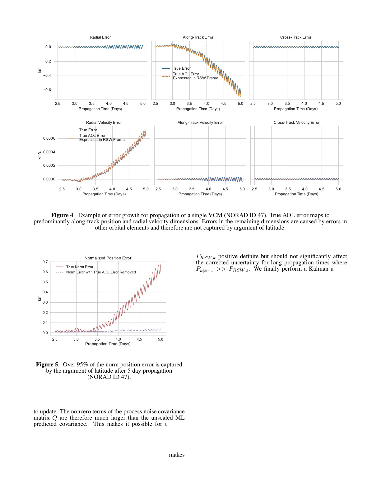
Machine Learning Argument of Latitude Error Model for LEO Satellite Orbit and Covariance Correction

Machine Lear ning Argument of Latitude Err or Model f or LEO Satellite Orbit and Cov ariance Correction Alex Moody Draper Scholar University of Colorado Boulder Boulder , CO alex.moody@colorado.edu Penina Axelrad University of Colorado Boulder Boulder , CO penina.axelrad@colorado.edu Rebecca Russell The Charles Stark Draper Laboratory , Inc. Cambridge, MA rrussell@draper .com Abstract— Low Earth orbit (LEO) satellites are le veraged to support new position, navigation, and timing (PNT) service alternati ves to GNSS. These alternati ves require accurate propagation of satellite position and v elocity with a realistic quantification of uncertainty . It is commonly assumed that the propagated uncertainty distribution is Gaussian; howe ver , the v alidity of this assumption can be quickly compromised by the mismodeling of atmospheric drag. W e de velop a machine learning approach that corrects error gro wth in the argu- ment of latitude for a diverse set of LEO satellites. The improved orbit propagation accurac y extends the applicability of the Gaussian assumption and modeling of the errors with a corrected mean and cov ariance. W e compare the performance of a time-conditioned neural network and a Gaussian Process on datasets computed with an open source orbit propagator and publicly av ailable V ector Cov ariance Message (VCM) ephemerides. The learned models predict the argument of latitude error as a Gaussian distribution giv en parameters from a single VCM epoch and re verse propagation errors. W e sho w that this one-dimensional model captures the effect of mismodeled drag, which can be mapped to the Cartesian state space. The correction method only updates information along the dimensions of dominant error growth, while maintaining the physics-based propagation of VCM cov ariance in the remaining dimensions. W e therefore e xtend the utility of VCM ephemerides to longer time horizons without modifying the functionality of the existing propagator . T A B L E O F C O N T E N T S 1 . I N T R O D U C T I O N . . . . . . . . . . . . . . . . . . . . . . . . . . . . . . . . . . . 1 2 . P RO PAG A T I O N E R R O R D AT A S E T G E N E R A T I O N . . 2 3 . A R G U M E N T O F L A T I T U D E E R RO R M O D E L I N G . . 3 4 . M AC H I N E L E A R N I N G A P P R OAC H . . . . . . . . . . . . . . . . 5 5 . E X P E R I M E N T A L R E S U L T S . . . . . . . . . . . . . . . . . . . . . . . . 7 6 . D I S C U S S I O N . . . . . . . . . . . . . . . . . . . . . . . . . . . . . . . . . . . . . . 9 7 . C O N C L U S I O N S . . . . . . . . . . . . . . . . . . . . . . . . . . . . . . . . . . . . 10 A C K N OW L E D G E M E N T S . . . . . . . . . . . . . . . . . . . . . . . . . . . . . . 10 R E F E R E N C E S . . . . . . . . . . . . . . . . . . . . . . . . . . . . . . . . . . . . . . . . 10 B I O G R A P H Y . . . . . . . . . . . . . . . . . . . . . . . . . . . . . . . . . . . . . . . . . 11 1 . I N T R O D U C T I O N Positioning, na vigation, and timing (PNT) using global na v- igation satellite systems (GNSS) is susceptible to jamming, spoofing, and signal degradation. These limitations have driv en the dev elopment of alternati ve PNT methods le ver - 979-8-3315-7360-7/26/ $31 . 00 ©2026 IEEE 𝛿𝑢 Pro p ag at e d M e an C or rec t e d M e an Pro p ag at e d C ov ar ian c e Co rr e c te d Co v arian c e Arg u m e n t of lat it u d e c or rec t ion 𝛿𝑢 𝑢 A s c ending N ode Figure 1 . Machine learning model predicts errors and variance in the ar gument of latitude to correct both the propagated orbit and cov ariance for a variety of LEO orbit and satellite types. aging Lo w Earth Orbit (LEO) satellites that were not de- signed for PNT . Unlike conv entional satellite-based navi- gation systems, these non-cooperativ e satellites do not em- bed ephemerides in their transmitted signal. Users of non- cooperativ e LEO satellite transmissions must therefore obtain the satellite ephemerides by other means, such as using acti ve radar tracking or passi ve tracking of the signal transmission from known locations. Regardless of the source, updated ephemerides must be downloaded from the tracking service provider and propagated to the time of measurement. The resulting PNT solution accuracy is therefore driven by the orbit propagation accuracy since the last ephemerides up- date. Improved propagation accuracy over long time horizons would reduce the required ephemerides update frequenc y and improv e the robustness of the alternati ve PNT system. Machine learning (ML) techniques are attractiv e for improv- ing orbit prediction accuracy because they are well suited to learn the complex patterns in propagation errors giv en ample historical tracking data [1]. A common hybrid ML approach uses the output of the machine learning model to correct 1 an existing orbit propagator . Peng and Bai ha ve explored using support vector machines, artificial neural networks (ANNs), and Gaussian processes (GPs) to forecast errors in two line element (TLE) ephemerides propagated with the simple general perturbations model 4 (SGP4) propagator [2]. They de veloped an approach to fuse the propagated solution with the machine learning model output using an Extended Kalman Filter and Particle Filter [3][4], assuming both the propagated and correction uncertainty can be trusted. The y tested their approach on a real TLE dataset containing 111 satellites in dif ferent orbital regimes by training a model for each satellite and error dimension in the local orbit frame defined by the radial, along-track and cross-track axes (RSW) [5]. These works demonstrated the practicality and power of the hybrid ML approach, b ut do not focus on generalization of a single model across different satellite types and orbits. In addition, they do not consider how inaccurately propagated cov ariance would affect the fusion approach or how to fore- cast correlations between error dimensions. Sev eral recent works [6][7] hav e focused on generalization across the Starlink constellation using the framework devel- oped by Peng and Bai. These works demonstrated improv ed SGP4 orbit propagation accuracy using a time delay neural network (TDNN) and ANN to predict corrections in all six position and v elocity dimensions for 1 hour and 3.5 day prop- agation windows, respectiv ely . Ho wev er, these methods do not predict corrections to the propagated cov ariance. Further- more, all Starlink satellites hav e similar physical characteris- tics and orbit shapes, reducing the generalization complexity . W e build upon this prior work by expanding the training dataset to include a wide variety of LEO satellites with dif- ferent physical characteristics, orbit sizes, and orbit shapes. Furthermore, our work is the first to extend the hybrid ML approach to more accurate ephemerides produced by the Space Force [8] in vector co variance message (VCM) format [9] and a special perturbations (SP) propagator . By extend- ing the hybrid approach to more accurate ephemerides and propagators [10], we focus on improving orbit and cov ariance accuracy over a week-long time horizon. Additionally , we simplify the modeling approach from prior work by only predicting corrections for the dominant error growth in LEO, which accumulates in the argument of latitude (A OL) dimen- sion (as illustrated in Figure 1). Finally , we correct along dimensions with the most se vere mismodeling by mapping the one dimensional model outputs to the Cartesian frame. This correction includes the mismodeled correlation terms in the covariance matrix. Figure 2 shows how the VCMs, machine learning models, orbit propagator , and correction approach work together to improv e orbit propagation. Section 2 discusses the public VCM dataset and how it is used with the SP propagator to compute propagation errors. Section 3 discusses the mapping of ar gument of latitude error and variance to the Cartesian frame. Section 4 discusses the feature set and ML models used. Finally , Section 5 discusses the performance of the models and correction approach using 1000 LEO satellites ov er a sev en day forecasting window . 2 . P R O PAG AT I O N E R R O R D AT A S E T G E N E R AT I O N VCM Dataset The VCM dataset used in this work was originally cre- ated by the United States Space F orce Space Command (USSP A CECOM) and was distributed publicly by Lav ezzi et Vecto r Co va r ia n ce M ess a ges      VCM Fea t ur e Ext r a ct ion Ma ch in e L ear n in g M o d el SP Or b it Pr o p a ga t o r                       AOL Co r r ect ion     ,       Figure 2 . Orbit propagation correction pipeline using VCMs, open source SP propagator , and machine learning model. T able 1 . Summary of VCM parameters used in modeling and dataset generation Parameter Description Epoch time (UTC) Orbital estimate epoch time, ex- pressed in Coordinated Univ er- sal T ime. J2K Pos/V el X-Y -Z ( k m , km/s ) The position and velocity vector components of the satellite ex- pressed in Earth-Centered Iner- tial reference frame. Ballistic Coef. ( m 2 /k g ) Estimated ballistic coef ficient at epoch. Solar Rad Press Coeff ( m 2 /k g ) Estimated solar radiation pres- sure coefficient at epoch. Geo Pot Degree and order of geopoten- tial model used. Drag Atmospheric density model used. F10, F10A F10 (10.7 cm) solar flux at epoch time and 81-day average solar flux. Sigma U-V -W -Ud-Vd-Wd ( k m , km/s ) Estimated position and veloc- ity error standard de viations in RSW Frame. al, [11] with permission. Each VCM contains state informa- tion for satellites at a single epoch, along with parameters used in the dynamics models for propagation and orbit deter- mination. The original dataset contains 22,303 resident space objects (RSOs) spanning various types of satellites and orbits. T able 1 describes the VCM fields used in our approach. An important limitation of the public dataset is that it only provides the estimation error standard de viations for position and velocity instead of a full covariance matrix. Furthermore, the VCMs truncate most velocity sigmas to zero because they only pro vide 0.1 m/s precision. W ithout correlations and valid velocity uncertainty , the propagated covariance is expected to be significantly inaccurate. Nev ertheless, the position sigmas provide an approximate initial uncertainty 2 500 1000 1500 2000 Orbit A titude ( km ) 10 −11 10 −9 10 −7 10 −5 10 −3 Acce erations ( km / s 2 ) O r b i t P e r t u r b a t i o n s F or ces SRP J2 So id T ides Sun Moon Drag R e ativit( A bedo Earth GM Figure 3 . Accelerations due to individual force models in Orekit orbit propagator ov er various altitudes for an example satellite in an initially circular orbit with a ballistic coefficient of 0.13 m 2 /k g . that can be used for a preliminary analysis of our covariance correction approach. W e reduced the full dataset to a list of 2,486 LEO satellites using information from Space Track. The list of all LEO satellites currently in orbit 2 was first downloaded from Space T rack and then filtered to those satisfying the following criteria: • Classified as having a large radar cross section (RCS) by Space T rack • Perigee altitude less than 1200 km • Not classified as ”Debris” • Not Starlink or OneW eb Large RCS satellites are chosen because they are easier to track with ground stations. W e also set a perigee altitude threshold of 1200 km to focus on satellites most affected by mismodeled atmospheric drag. Figure 3 shows ho w the mag- nitude of the atmospheric drag perturbation increases rapidly as the orbital altitude decreases below 1200 km. W e also remov e the maneuvering OneW eb and Starlink constellations in this study to explore generalization across satellites with natural dynamics. Although other active payloads besides Oneweb and Starlink maneuver , removing the lar ge constel- lations helps increase the percentage of non-maneuvering satellites in the dataset. This list is reduced further to 1,000 objects by removing the remaining maneuv ering satellites. Pr opagator Setup The Orekit [12] open source orbit modeling software is used to propagate the VCM states and cov ariances. The propagator is configured to closely match the dynamic models in the VCM files. The force models shown in T able 2 are inte grated with Dormand-Prince 8(5,3) [13] to propagate each set of VCM initial conditions. By using a high order gravity model and including other significant perturbations in LEO orbit, errors in drag modeling are left as the most significant error 2 https://www.space- track.org/basicspacedata/query/ class/satcat/PERIOD/< 128/DECAY/null- val/CURRENT/Y/ format/csv T able 2 . Orekit Force Models Perturbation For ce Models Solar Radiation Pressure 70 × 70 Gravity (EGM-96) Solid Earth T ides Sun Third Body Moon Third Body Atmospheric Drag (NRLMSISE-00) Relativity Albedo (Knocke) source in the propagator . The ballistic coefficients B C provided in the VCMs are used to initialize the drag model for each satellite. Orekit has separate parameters for the coef ficient of drag, cross sectional area, and mass. The ballistic coef ficient is split up into these parameters by fixing the satellite mass m and adjusting the cross sectional area A to be consistent with the ballistic coefficient B C provided in each VCM epoch: A = mB c C d (1) where C d is fixed at 2.2. This method was compared with using masses from the DISCOS [14] dataset and similar propagation performance was observ ed. The propagator state is initialized using the position and velocity provided for a VCM epoch. Gi ven the velocity sigma values in the VCMs are generally truncated to zero, we set them to the largest value that would not be captured using the file precision. The initial cov ariance is therefore likely to be somewhat conservati ve, giv en the inflation of the velocity sigmas and assumption of no correlation between states in the RSW frame. Pr opagation Err or Computation The propagation errors are computed by initializing the prop- agator at one VCM epoch and propagating forward to future VCM epochs. The VCM states and propagated states are then con verted to osculating orbital elements from Earth Centered Inertial (ECI) positions and velocities. The argument of latitude errors are computed by differencing the osculating orbital elements at each VCM epoch in a 7 day window . The VCM epochs are asynchronous across satellites, so the com- puted errors do not hav e common timestamps or frequency . Although this error computation ignores noise in the refer- ence states, it is a valid approximation, giv en that the VCM uncertainties are small relativ e to the systematic orbit errors we observe after 1.5 days of propagation. The median norm position standard deviation reported in the VCMs used for this study is 14.7 meters, which is significantly less than the 134.5 meter median norm propagation error between 1-1.5 days. 3 . A R G U M E N T O F L AT I T U D E E R R O R M O D E L I N G Although LEO SP propagators can lev erage more accurate force models than SGP4, they are still limited by mismodeled 3 atmospheric drag [15]. Drag force mismodeling is caused by errors in the satellite specific ballistic coefficient and atmospheric density models. Operational semi-empirical atmospheric density models such as NRLMSISE-00 and JB2008 fit an analytical model to historical calibration data to forecast atmospheric densities [1]. These models are especially inaccurate at forecasting density during periods of high solar acti vity [16]. The drag force primarily acts opposite to the direction of spacecraft motion, causing errors to accumulate in the argument of latitude when expressed in orbital elements. By modeling errors in the argument of latitude, we capture the dominant error growth in position and velocity with a single dimension. State T ransformation Hayek and Kassas provide a conv enient transform of errors in the argument of latitude to the RSW frame [17]. The y only consider the argument of latitude error because other orbital elements will accumulate errors at a much slower rate. Therefore, propagated orbital elements are used to map the error in ar gument of latitude ( δ u ) to RSW errors. Since the argument of latitude defines a spacecraft position along an orbit, it can only be used to capture errors in the orbit plane. Equation 2 shows no errors are mapped to the orbit normal direction for both position and velocity . δ X RS W =   r (1 − cos δ u ) r { 2 sin δ u − e [sin( ω − u − 2 δu ))+sin( u − ω )] } 2( e cos ( u − ω )+1) 0   (2) δ ˙ X RS W =   − µ h sin( δ u ) µ {− 2 cos δ u +2+ e [ − cos( ω − u − 2 δ u )+2 cos( δ u + u − ω ) − cos ( u − ω )] } 2 h ( e cos ( u − ω )+1) 0   (3) where µ is the gravitational parameter for Earth and e, u, ω , f , h are the osculating eccentricity , argument of lat- itude, argument of perigee, true anomaly and angular mo- mentum for the propagated state. The argument of latitude correction error uncertainty is mapped to the RSW and ECI coordinate frames with Λ ∆ =  ∂ δ X RS W ∂ δ u ∂ δ ˙ X RS W ∂ δ u  =                   r sin( δ u ) r { cos δu + e cos( ω − u − 2 δ u )) } ( e cos f +1) 0 − µ h cos( δ u ) µ { sin δu − e [sin( ω − u − 2 δu )+ sin ( δ u + u − ω )] } h ( e cos f +1) 0                   (4) P E C I = R RS W T E C I Λ P u Λ T R RS W E C I (5) where P u is the argument of latitude covariance, R RS W E C I is the rotation matrix from ECI to RSW and P E C I is the argument of latitude variance e xpressed in the ECI frame. Corr ection Approac h Our approach corrects the dimensions most affected by drag mismodeling while maintaining accurate propagation infor- mation in the remaining dimensions. Figure 4 shows how the true ar gument of latitude error mapped to the RSW frame captures the secular drift in along-track position and radial velocity . Although the argument of latitude error also maps to the radial position and along-track velocity , it is not re- sponsible for the dominant error growth in those dimensions. Errors in other orbital elements create zero mean oscillations with slowly growing amplitudes. In Figure 5 we show ho w subtracting the mapped true argument of latitude error from the propagated states reduces most of the error for a LEO satellite. For instance, by removing the drift in the along- track dimension, we reduce the norm position error by over 95%. W e therefore only correct the mar ginal distrib ution of the along-track position and radial velocity v ariables. W e modify the fusion approach presented in [3] to account for scenarios where the propagated cov ariance is inaccurate. When the propagator does not properly account for process noise, the propagated covariance becomes unrealistic, and typically overconfident. If the propagated covariance is ov erconfident and a Kalman update is performed with the ML output, the propagated state would be weighted hea vier than the ML correction. W e instead inflate the cov ariance in the along-track position and radial velocity dimensions before performing the Kalman update. This allows for the ML model to inflate the cov ariance if necessary . Consequently , the ML model must output variances consistent with its error predictions for this method to be robust. The propagated state and cov ariance in ECI are defined as X k | k − 1 , P k | k − 1 (6) where X k | k − 1 is a 6 × 1 matrix and P k | k − 1 is a 6 × 6 matrix. The one dimensional predicted argument of latitude error and uncertainty are δ u k , P u,k (7) The propagated state is corrected with the ML predicted error to get a new state estimate ˆ X k . P k | k − 1 is inflated along the correction axes with a scaled version of the ML predicted cov ariance P RS W,k . δ u → δ X RS W , δ ˙ X RS W (computed with (2) & (3)) ˆ X k | k = X k | k − 1 + R RS W T E C I  δ X RS W δ ˙ X RS W  k (8) P RS W,k = Λ P u Λ T + P RS W, 0 (9) Q = α diag (0 , 1 , 0 , 1 , 0 , 0) P RS W,k diag (0 , 1 , 0 , 1 , 0 , 0) (10) P k | k − 1 = P k | k − 1 + Q (11) where α is a scale factor we set to 1e6 and the diagonal matrices are used to select the marginal distribution we want 4                                                                                                         Figure 4 . Example of error growth for propagation of a single VCM (NORAD ID 47). T rue A OL error maps to predominantly along-track position and radial velocity dimensions. Errors in the remaining dimensions are caused by errors in other orbital elements and therefore are not captured by argument of latitude.                                     Figure 5 . Over 95% of the norm position error is captured by the argument of latitude after 5 day propagation (NORAD ID 47). to update. The nonzero terms of the process noise cov ariance matrix Q are therefore much larger than the unscaled ML predicted cov ariance. This makes it possible for the ML cov ariance update to inflate the propagated cov ariance. Fur- thermore, the initial VCM cov ariance is combined with the predicted cov ariance because mapping one dimensional vari- ance into multiple dimensions through a linear transformation creates a singular matrix. Adding the initial cov ariance makes P RS W,k positiv e definite but should not significantly affect the corrected uncertainty for long propagation times where P k | k − 1 >> P RS W, 0 . W e finally perform a Kalman update with the ML predicted cov ariance. H =  0 1 0 0 0 0 0 0 0 1 0 0  R RS W E C I (12) P r ˙ s,k =  P RS W,k (2 , 2) P RS W,k (2 , 4) P RS W,k (4 , 2) P RS W,k (4 , 4)  (13) K = P k | k − 1 H T ( H P k | k − 1 H T + P r ˙ s,k ) − 1 (14) ˆ P k | k = ( I − K H ) P k | k − 1 ( I − K H ) T + K P r ˙ s,k K T (15) where P r ˙ s,k is the 2 × 2 mar ginal distribution of P RS W,k in the along-track position and radial velocity . The measure- ment matrix H maps the propagated cov ariance to this two dimensional frame. W e therefore correct the mismodeled components of the distribution without corrupting accurately propagated information in other dimensions. 4 . M A C H I N E L E A R N I N G A P P RO AC H W e considered two machine learning models for forecasting argument of latitude errors. The first is a time-conditioned feed forward neural network (TCNN) [18], and the second is a heteroscedastic Gaussian process (HGP) [19]. These two 5 models predict means and cov ariance values, allowing us to compare the performance of non-parametric and parametric models for this regression problem. F eature Extraction The selection of features was an iterati ve process through test- ing on smaller datasets and monitoring model performance. Orbital elements used as features were deriv ed from VCM positions and velocities. The features used in the NN are as follows: • Reverse propagation times and along-track errors up to 2 days in the past • Altitude at perigee • Eccentricity • cos( f ) • cos( i ) • B C (VCM Parameter) • F 10 . 7 A (VCM Parameter) • Payload Classification (one-hot encoding) • Rocket Body Classification (one-hot encoding) • ∆ t prop where f is the propagated true anomaly and i is the prop- agated inclination. The cosine is taken of true anomaly to encode distance from perigee or apogee. For eccentric orbits, the propagation error will expand around apogee and shrink around perigee due to orbital dynamics. The cosine is also taken of inclination to map the angle to a value between -1 and 1. Since the VCM epoch spacing differs between satellites, a maximum of 11 epochs in the reverse direction are used to generate features. Satellites that do not have 11 epochs within the 2 day windo w are padded with re verse propag ation errors of zero at time zero. Additionally , the payload and rocket body classifications are pulled from DISCOS and are binary values to encode the satellite type. The 11 rev erse propagation errors, 11 rev erse propagation times, and the 9 other v ariables add up to a feature vector with 31 dimensions. Although HGPs are technically non-parametric, they still require optimization of the kernel function parameters that define the cov ariance functions between data points. The training of a GP has computational complexity of O ( n 3 ) and prediction has computational complexity of O ( n 2 ) [20]. T o reduce the computational load of the HGP , only the longest rev erse propagation epoch is used as a feature, along with altitude at perigee, B c and ∆ t prop . W e arrived at this subset of features through multiple rounds of training and testing the HGP . T ime-Conditioned F eed F orwar d Neural Network The TCNN consists of an input layer, two hidden layers and one output layer . The output layer is a univ ariate Gaussian characterized by the output mean and variance. Each hid- den layer has 128 dimensions and the input layer has 31 dimensions. W e train the TCNN on the argument of latitude propagation error using Gaussian maximum likelihood. The predicted argument of latitude error is assumed to follow a normal distribution δ u ∼ N ( µ δ u , P u ) . The probability density function for the univ ariate Gaussian is p ( δ u | z ) = 1 p 2 π σ ( z ) 2 exp  − ( δ u − f ( z )) 2 2 σ ( z ) 2  (16) where f ( z ) is the learned mean function and σ ( z ) is the learned v ariance function. W e define our loss function L as the negati ve logarithm of the univ ariate Gaussian likelihood. W e train the model by minimizing the loss function through gradient decent and optimize f and σ simultaneously . L = 1 2  ( δ u − f ( z )) 2 σ ( z ) 2 + ln σ ( z ) 2  (17) W e use an exponential activ ation function for the output variance to stabilize training [21]. Heter oscedastic Gaussian Pr ocess The general expression for a GP is given by Rasmussen [22] as, f ( x ) ∼ G P ( m ( x ) , k ( x, x ′ )) (18) where we define the mean function m ( x ) as zero [22]. The kernel function k ( x, x ′ ) defines the cov ariance between two function outputs. Basis functions are typically chosen to produce higher correlation v alues for inputs that are closer together . W e use the common Gaussian basis function. k ( x i , x j ) = exp  − ( x i − x j ) 2 θ  (19) where θ is the length scale for the basis functions. The cov ariance matrix for the GP consists of an N × N matrix where each element ( i, j ) contains the output of the kernel function for the inputs x i , x j . F or a GP with zero mean, the cov ariance matrix fully defines the joint distribution of all function outputs. Giv en a set of observations Y and features X , the predic- tiv e distribution can be found by first estimating the kernel function parameters. They can be found by maximizing the log likelihood function log p ( Y | X , θ ) . Once the parameters are determined, test features x ∗ can be added to the GP cov ariance matrix using the kernel function to correlate x ∗ with all other inputs. The predicti ve distribution is therefore giv en by the conditional probability of y ∗ giv en Y . Since all of the function outputs are jointly Gaussian, the conditional distribution will also be Gaussian and is gi ven by equation 20 and 21 µ ∗ = k ( x ∗ , X )[ K + β − 1 I ] − 1 Y (20) where k ( x ∗ , X ) is the covariance function ev aluated with x ∗ and all other inputs in training set X . β is the precision term representing the constant noise on the observations. σ 2 ∗ = k ( x ∗ , x ∗ ) − k ( x ∗ , X )[ K + β − 1 I ] − 1 k ( X, x ∗ ) (21) The adv antage of GP prediction is that it naturally accounts for epistemic uncertainty . If an input feature vector is far from all of the feature vectors in the model, then the GP would predict an output distribution with lar ge variance. W e also recognize that random modeling errors accumulate during propagation and create noise distributions as a func- tion of the propagation time. W e show an example of the varying noise profile for ar gument of latitude errors in Figure 6. W e therefore use a heteroscedastic Gaussian Process to model the noise with a latent GP . W e use the hetGPy python package for an optimized het- eroscedastic GP framew ork [23]. The package extends the hetGP R package that is designed to handle large datasets through efficient use of replicated inputs [24]. Although 6 Figure 6 . A OL errors used to train the ML models consisting of 50 VCMs propagated 7 days for 800 satellites. the input data is unlikely to hav e many exact replicates due to continuous scales on most input features, the package is efficient at optimizing the hyperparameters for lar ge datasets. Even with the optimized software, training the model with the full dataset and feature list is prohibitiv ely slo w . W e discuss the compromises made during GP training in the following section. 5 . E X P E R I M E N TA L R E S U LT S The machine learning models are trained on data from 800 satellites randomly picked from the 1000 satellite dataset. They are tested on data from the remaining 200 satellites cov ering the same time window . This split of the training and v alidation data allo ws for testing of generalization across satellite orbits and physical characteristics while ignoring temporal ef fects on orbit propagation. Generalization to future time windo ws is briefly in vestigated; howe ver , it will be the focus of future work. W e test each model by predicting argument of latitude errors for v alidation feature vectors. The prediction error is the difference between the model output and the v alidation tar get errors. The prediction error is then compared with the model predicted cov ariance. The model prediction means and variances are mapped to the Cartesian RSW frame where the correction approach described in section 3 is applied. W e then present the improvements made by the model corrections to the true error distribution and co variance realism. All features and labels except for the satellite type classifica- tions are normalized with the mean and standard deviation of the training dataset. x normal ized = x − µ x σ x (22) where x is a feature variable, µ x is the mean of x in the training data, and σ x is the standard deviation of x in training data. During prediction, input features and output error predictions are normalized using the µ x and σ x computed with the training set. T able 3 shows the uncorrected error standard deviations for the training dataset. As expected, most of the error is in the along track position and radial v elocity dimensions. The error T able 3 . V alidation dataset standard deviations in RSW frame after sev en days of propagation σ R r km σ R s km σ R w km σ V r m/s σ V s m/s σ v w m/s 0.23 12 0.013 13 0.043 0.017 3 4 5 6 7 P r o p a g a t i o n T i m e ( D a y s ) − 0 . 0 1 0 − 0 . 0 0 5 0 . 0 0 0 0 . 0 0 5 0 . 0 1 0 0 . 0 1 5 A g u m e n t o f L a t i t u d e P o p a g a t i o n E o ( R a d ) C o e c t e d U n c o e c t e d Figure 7 . TCNN - Corrected and Uncorrected Error Distributions Ov er Time. in the remaining four dimensions is at least two orders of magnitude smaller . Neural-Network P erformance The TCNN was trained using an Adam optimizer [25] with a learning rate of 1 e − 3 and a batch size of 50,000. W e first compare the corrected A OL error distrib ution to the uncorrected A OL distribution for each day of propagation in Figure 7. Unlike a traditional box plot that only shows four quantiles, the enhanced box plot displays quantiles about the mean decreasing by a factor of two [26]. For instance, the innermost box es represent the 25 and 75 percentiles followed by a set of boxes drawn at the 12.5 and 87.5 percentiles. The extreme points are defined as 3/2 times less than than the lower quantile or 3/2 times greater than the upper quantile. The enhanced box plot sho ws how the uncorrected true error distribution is ske wed in the positive direction and contains extremely long tails. The ML corrections not only improve the ske wness but reduce the long tails and spread of the distribution. Figure 8 shows a corner plot of the uncorrected and corrected error distributions in the Earth Centered Inertial (ECI) Carte- sian frame. Each histogram along the diagonal represents the error distribution in one of the six error vector dimensions. The two dimensional marginal distributions for all combina- tions of v ariables are sho wn in scatter plots. All of the scatter plots and histograms in the same column have the same x values and all scatter plots in the same ro w hav e the same y values. The histograms also match the y values for the scatter plots sharing the same row . W e see here how the one dimensional argument of latitude correction maps to the six dimensional ECI Cartesian state space. The uncorrected distribution is non-Gaussian in many 7 40 20 0 20 Y (km) 40 20 0 20 Z (km) 40 20 0 20 Vx (m/s) 20 0 20 40 V y (m/s) 25 0 25 X (km) 40 20 0 20 40 Vz (m/s) 25 0 25 Y (km) 50 25 0 25 Z (km) 40 20 0 20 Vx (m/s) 25 0 25 V y (m/s) 50 0 50 Vz (m/s) Cor r ected Uncor r ected Figure 8 . TCNN - Error reduction in all dimensions of ECI Cartesian frame after A OL correction. marginal distributions. The histograms sho w how the spread of the errors decreases in ev ery dimension with the orbit corrections, resulting in tighter and more Gaussian marginal distributions. Gaussian Pr ocess P erformance In addition to decreasing the number of features as discussed in section 4, we retain every 1,000th sample from the dataset to reduce the memory requirements of the model. This down selection process ensured samples from each satellite remained in the training set. Ho wev er, it did not ensure that there were samples from ev ery satellite every day . W e chose to downsample the dataset by the factor of 1,000 after a few iterations showed it had the best balance of computational resources and performance. T able 4 shows the performance of the HGP compared with the TCNN and uncorrected distributions; where σ R s and σ V r are the standard deviation of the along-track position errors and radial velocity errors, respecti vely; σ ∥ R ∥ and σ ∥ V ∥ are the standard deviation of the norm position and velocity errors, respectiv ely; % D M u ,C is the percent of Mahalanobis distance samples that are less than a consistency threshold in the argument of latitude dimension; and % D M [ R,V ] ,C is the same metric but for position and v elocity in ECI. The consistenc y threshold for % D M u ,C and % D M [ R,V ] ,C is set at the 99th percentile of the χ 2 distribution for one and six degrees of freedom, respectiv ely . It follo ws that if the reported consistency metric is less than 99%, there are more distances abov e the threshold than in the theoretical distribution. The cov ariance would therefore be overconfident more often than expected. If the reported consistency metric is over 99%, the cov ariance would be underconfident more often than expected. The first line of T able 4 shows the uncorrected values. W e compute % D M [ R,V ] ,C with the uncorrected errors and co- variances to show the consistency of the propagator output. Only 7.7% of the uncorrected Mahalanobis distance samples are under the consistency threshold. This is not surprising giv en that process noise is not included and the limited initial cov ariance information av ailable in the public VCM dataset. The final two lines in T able 4 show the same metrics after correcting the errors and co variances with the model out- puts. The corrections from both machine learning models reduce the error sigmas by approximately a factor of two, while increasing the consistency metric from 7.7% to ov er 80%. Although this suggests that the corrected cov ariance is still somewhat overconfident, the correction significantly improv es the co variance consistency . Furthermore, the con- sistency of the one dimensional model outputs are very close 8 T able 4 . Correction performance for HGP and TCNN for 7 day propagation Dataset σ R s km σ V r m/s σ ∥ R ∥ km σ ∥ V ∥ m/s % D M u ,C % D M [ R,V ] ,C Uncorrected 12 13 11 12 - 7.7 TCNN 6.2 6.8 5.5 6.1 95 81 HGP 6.8 7.5 6.1 6.7 97 81 0 5 10 15 20 25 30 Squar ed Mahal anobis Di stance 0.0 0.2 0.4 0.6 0.8 1.0 P r obabil ity 6 DOF Squar ed M a h a l a n obis D ista n c e CD F - 7 Day P r opag ation Uncor r ected T CNN HGP Chi-Squar ed Theor et ical Distr ibu ti on Figure 9 . Cov ariance realism improv ement after A OL correction in ECI Cartesian frame. to matching the theoretical distribution. Both models have ov er 95% of the argument of latitude Mahalanobis distance samples within the consistency threshold. The v ariance out- put by the models is therefore mostly consistent with the true argument of latitude errors, but the mapping to ECI position and velocity cannot correct for all of the inconsistencies in the propagated cov ariance. Figure 9 shows the Mahalanobis distance empirical CDF for the uncorrected, TCNN and HGP results in addition to the theoretical chi-squared distribution for six degrees of freedom. The empirical Mahalanobis distance distrib ution should match the shape of the theoretical distribution if the errors are normally distributed and the variance is scaled correctly . W e see that the uncorrected CDF does not follo w the theoretical distribution and contains many samples with large Mahalanobis distances. The corrected CDFs using the TCNN and HGP have similar performance and are closer to following the theoretical distrib ution. V alidation using Future Epochs W e also in vestigate the generalization of the HGP and TCNN models ov er time and satellites. W e tested time generalization with a validation dataset that contains the same satellites as the original validation dataset, but uses future VCMs to generate the errors. The training dataset therefore does not contain any of the satellites in the v alidation dataset nor any data for the same time window as the validation dataset. T able 5 shows ho w the two models generalize ov er time. The models still improv e the orbit accuracy , but by less than 2 km in position and 2 m/s in velocity . Additionally , the consistency of the TCNN predicted v ariance is 63.9%, versus 95.3% without time generalization. The HGP consistency , howe ver , only decreases by 1.2%. This is due to the inherent ability of Gaussian processes to inflate uncertainty when test samples do not closely align with the training data. 6 . D I S C U S S I O N The experimental results for HGP and TCNN corrections show that both models are capable of improving the orbit and covariance accuracy . The prediction accuracy of both models is very similar . They are within 1 km of each other for position and 1 m/s for velocity . The v ariance prediction accuracy metric is also within 1% for the two models. While both models reduce the position and velocity error standard deviation by about 50%, there are still areas of impro vement. Giv en the HGP model achieved similar performance to the TCNN using only 0.1% of the training dataset and less than half the feature variables, we likely could reduce the feature set used in the TCNN and increase the size of the training dataset to enable more optimization epochs without overfit- ting. Furthermore, gradient descent may not find optimal mean predictions when using heteroscedastic Gaussian loss due to under weighting of points that are difficult to model [27]. Seitzer et al. [27] suggest using a scale factor in the loss function to adjust the dependence of the gradients on predictiv e variance. This method could help improve the mean prediction accuracy while still optimizing the v ariance function. The HGP model suffered from computational complexity of the lar ge training dataset. Sparse HGPs, such as the one used in [5], optimize a subset of feature vectors that best approximate the larger dataset. This method allo ws for more data to be used to train the model without scaling up the computational complexity . The challenge with this method is that the training process is more complex since both the primary feature vectors and the kernel parameters must be optimized simultaneously . Giv en the promising performance of the HGP using a naiv e downsampling of the full dataset, a sparse method trained on the full dataset could perhaps improv e its orbit prediction accuracy . The cov ariance corrections from both models generated Ma- halanobis distance distributions that were closer to the theo- retical χ 2 distribution than the uncorrected distribution. As discussed in section 2, the VCM dataset only contains valid position standard deviations. The true cov ariance matrix for the VCM initial conditions likely contains correlations and velocity sigmas that would be necessary for an accurate representation of the initial uncertainty . Ultimately , we show promising improv ements to covariance realism with our ap- proach but should validate the approach with full covariance information before integration into a na vigation filter . For practical integration of our approach into a navigation pipeline, the machine learning models need to generalize 9 T able 5 . Correction performance for HGP and TCNN for 7 day propagation with time generalization Dataset σ R s km σ V r m/s σ ∥ R ∥ km σ ∥ V ∥ m/s % D M u ,C Uncorrected 12 13 11 12 - TCNN 11 12 11 12 64 HGP 9.9 11 9.3 10 96 well to new satellites and future VCM epochs. The models trained in this work do not generalize ov er new VCM epochs most likely due to the limited windo w of time the training set covers. Depending on the tracking frequency for each satellite the training dataset only spans 1-2 weeks. The training set is therefore unlikely to capture temporal changes to orbit propagation accuracy leading to significant epis- temic uncertainty . This is most likely the reason the TCNN was overconfident in its variance predictions. Ensembling approaches could be taken in future work to account for epistemic uncertainty in the TCNN [28]. Another challenge with generalization across time in LEO orbit propagation is the changes in space weather due to the solar c ycle. The solar cycle fluctuates every 11-years [29] and higher solar activity leads to larger errors in atmospheric density modeling [16]. It is impractical to maintain a dataset spanning the full solar cycle, howe ver , future work will inv estigate if training on a one or two month window improv es time generalization for VCM epochs immediately following the training data. Despite our improvements to orbit accuracy , we recognize that the corrected errors remain on the order of kilometers in the along-track position and meters per second in the radial velocity dimensions. W ithout further improv ements to the models, these errors alone are too large to meet typical PNT system requirements. The remaining dimensions, howe ver , hav e significantly better propagation performance and remain useful for navigation after a sev en day propagation. W ith enough geometric variation, the remaining four dimensions can pro vide accurate information for na vigation. When a filter ingests the propagated state information, it depends on the cov ariance to determine which dimensions are accurate. If the propagated covariance is over confident and the true error distribution is not Gaussian, the filter may fail to lev erage this accurate navigation information. The main benefit of our current correction performance is therefore improving the Gaussianity of the true error distrib ution and the cov ariance realism such that a navigation filter can safely ingest the propagated ephemeris. Finally , another practical application of the current mod- eling performance is to decide which satellites to use for navigation after long propagation times. Gi ven the trained model and at least two VCMs for a ne wly launched LEO satellite, maintainers of alternati ve PNT systems can predict the propagation accuracy . Giv en their mission and system requirements, they can add or reject the satellite from their catalog without additional analysis. T o improv e on this use case, future work will look at training models without re verse propagation errors as features. Therefore, only information from a single VCM epoch would be required to predict orbit propagation accuracy . 7 . C O N C L U S I O N S W e hav e explored using parametric and non-parametric ma- chine learning models to improv e orbit and cov ariance accu- racy for dif ferent LEO satellite types and orbits. By focusing on LEO, most of the propagation error is due to atmospheric drag mismodeling and therefore accumulates in the ar gument of latitude. Instead of training the model on the complex error distributions in the Cartesian frame, we perform regression with the one dimensional errors in the argument of latitude. The argument of latitude prediction from both models reduces the orbit position and velocity accuracy by approximately 50% for validation satellites disjoint from the training set. The TCNN produced more accurate orbit corrections than the HGP on validation data within the same time windo w as the training data. Ho wever , the HGP covariance predictions generalized better across time. Our method demonstrates the ability of a single model to impro ve orbit propagation for different LEO satellites. By improving the accurac y of orbit propagation, we e xtend the time windo w in which alternati ve PNT systems can lev erage VCMs for navigation. A C K N O W L E D G E M E N T S This work w as supported by The Charles Stark Draper Labo- ratory . R E F E R E N C E S [1] F . Caldas and C. Soares, “Machine learning in orbit estimation: A survey , ” Acta Astronautica , vol. 220, pp. 97–107, 2024. [2] H. Peng and X. Bai, “Comparativ e ev aluation of three machine learning algorithms on improving orbit predic- tion accuracy , ” Astr odynamics , vol. 3, no. 4, pp. 325– 343, 2019. [3] ——, “Fusion of a machine learning approach and classical orbit predictions, ” Acta astr onautica , v ol. 184, pp. 222–240, 2021. [4] ——, “Improving accuracy and precision through ma- chine learning fusion using two-line element sets, ” in AIAA SCITECH 2022 F orum , 2022, p. 0863. [5] ——, “A medium-scale study of using machine learning fusion to improve TLE prediction precision without external information, ” Acta Astr onautica , vol. 204, pp. 477–491, 2023. [6] P . E. K ouba, S. Hayek, J. Saroufim, Z. M. Kassas, and E. Fakhoury , “Improved Starlink satellite orbit predic- tion via machine learning with application to oppor- tunistic LEO PNT, ” in Pr oceedings of the 37th Inter- national T echnical Meeting of the Satellite Division of The Institute of Navigation (ION GNSS+ 2024) , 2024, pp. 2424–2433. [7] D. Huang, “ A neural network augmented approach to large-scale satellite orbit propagation, ” Master’ s thesis, Univ ersity of Southern California, 2025. [8] G. Lavezzi, “VCM dataset for the classification of 10 resident space objects, ” Oct. 2024. [Online]. A vailable: https://doi.org/10.5281/zenodo.13892132 [9] 18th Space Defense Squadron, “V ector Co vari- ance Message (VCM), ” https://zenodo.org/records/ 13892132/files/VCM readme.pdf . [10] D. Conke y and M. Zielinski, “ Assessing performance characteristics of the SGP4-XP propag ation algorithm, ” in Advanced Maui Optical and Space Surveillance T ech- nologies Conference , Maui, HI, USA , 2022. [11] G. La vezzi, P . Mun Siew , D. W u, Z. Folcik, V . Rodriguez-Fernandez, J. Price, and R. Linares, “Early classification of space objects based on astro- metric time series data, ” 25th Advanced Maui Optical and Space Surveillance T echnologies. Maui Economic Development Boar d, Maui , 2024. [12] L. Maisonobe, “CS-SI/orekit: 12.2, ” Oct. 2024. [Online]. A vailable: https://doi.org/10.5281/zenodo. 13950582 [13] ——, “Hipparchus-Math/hipparchus: Hipparchus 3.0, ” Oct. 2023. [Online]. A vailable: https://doi.org/10.5281/ zenodo.8418401 [14] H. Klinkrad, “DISCOS - ESA ’ s database and informa- tion system characterising objects in space, ” Advances in Space Resear ch , vol. 11, pp. 43–52, 1991. [15] V . Ray , D. J. Scheeres, S. Alnaqbi, W . K. T obiska, and S. G. Hesar , “ A framew ork to estimate local atmo- spheric densities with reduced drag-coefficient biases, ” Space W eather , v ol. 20, no. 3, p. e2021SW002972, 2022. [16] D. A. Brandt, C. D. Bussy-V irat, and A. J. Ridley , “ A simple method for correcting empirical model densities during geomagnetic storms using satellite orbit data, ” Space W eather , vol. 18, no. 12, p. e2020SW002565, 2020. [17] S. Hayek, J. Saroufim, and Z. M. Kassas, “ Analysis and correction of LEO satellite propagation errors with application to navig ation, ” in Pr oceedings of the 37th International T echnical Meeting of the Satellite Division of The Institute of Navigation (ION GNSS+ 2024) , 2024, pp. 1800–1811. [18] C. M. Bishop, P attern Recognition and Machine Learn- ing . Springer, 2006. [19] K. Kersting, C. Plagemann, P . Pfaf f, and W . Burgard, “Most likely heteroscedastic Gaussian process regres- sion, ” in Pr oceedings of the 24th international confer- ence on Machine learning , 2007, pp. 393–400. [20] H. V an Do, E. V azquez, and T . Q. Long, “Scalable gaussian process for lar ge datasets, ” in International W orkshop on AD V ANCEs in ICT Infrastructur es and Services , 2024. [21] R. L. Russell and C. Reale, “Multiv ariate uncertainty in deep learning, ” IEEE T ransactions on Neural Networks and Learning Systems , vol. 33, no. 12, pp. 7937–7943, 2021. [22] C. E. Rasmussen and C. K. I. Williams, Gaussian Pr o- cesses for Machine Learning . The MIT Press, 2006. [23] D. O’Gara, M. Binois, R. Garnett, and R. A. Hammond, “hetGPy: Heteroskedastic Gaussian process modeling in Python, ” Journal of Open Source Softwar e , vol. 10, no. 106, p. 7518, 2025. [24] M. Binois and R. B. Gramacy , “hetgp: Heteroskedastic Gaussian process modeling and sequential design in R, ” Journal of Statistical Softwar e , vol. 98, pp. 1–44, 2021. [25] D. P . Kingma and J. Ba, “ Adam: A method for stochas- tic optimization, ” arXiv e-prints , v ol. 2014. [26] M. L. W askom, “Seaborn: statistical data visualization, ” Journal of Open Source Software , vol. 6, no. 60, p. 3021, 2021. [Online]. A vailable: https://doi.org/10. 21105/joss.03021 [27] M. Seitzer, A. T av akoli, D. Antic, and G. Martius, “On the pitfalls of heteroscedastic uncertainty estimation with probabilistic neural networks, ” 2022. [Online]. A vailable: https://arxiv .org/abs/2203.09168 [28] A. Acharya, R. Russell, and N. R. Ahmed, “Learning to forecast aleatoric and epistemic uncertainties over long horizon trajectories, ” in 2023 IEEE International Con- fer ence on Robotics and Automation (ICRA) . IEEE, 2023, pp. 12 751–12 757. [29] NOAA Space W eather Prediction Center, “Solar Cycle Progression, ” Sep. 2025, (accessed Sep. 15, 2025). [Online]. A v ailable: https://www .swpc.noaa. gov/products/solar - cycle- progression B I O G R A P H Y [ Alex Moody received his B.S. in Engi- neering from Harvey Mudd College and is currently a graduate student researcher in the Colorado Center for Astrodynam- ics Research at University of Colorado, Boulder . His research is funded by Draper and focuses on navigation util- ity of LEO satellites. Prior to graduate studies, he spent four years dev eloping navigation systems at Draper . P enina Axelrad is a Distinguished Pro- fessor in Aerospace Engineering Sci- ences at the Univ ersity of Colorado Boulder . Her research interests include GNSS-based and alternativ e positioning, navigation, and timing techniques. Dr . Axelrad is a Fellow of the Institute of Navigation and the AIAA, and a Mem- ber of the National Academy of Engi- neering. Rebecca Russell is a Principal Member of the T echnical Staff in the Percep- tion and Embedded Machine Learning Group at Draper . She joined Draper in 2016 after receiving her Ph.D. from MIT and B.S. from Caltech. At Draper , Dr . Russell’ s research focuses on using uncertainty-aware deep learning to solv e challenges in autonomy and navig ation. 11