Certifying Hamilton-Jacobi Reachability Learned via Reinforcement Learning

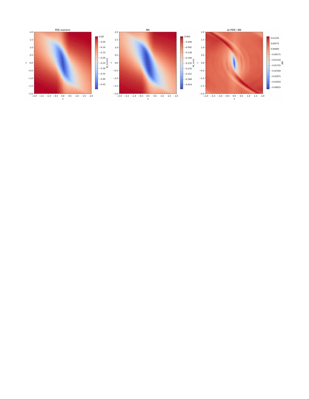
JOURNAL OF L A T E X CLASS FILES, VOL. 14, NO. 8, A UGUST 2021 1 Certifying Hamilton-Jacobi Reachability Learned via Reinforcement Learning Prashant Solanki 1 , Isabelle El-Hajj, Jasper J. v an Beers, Erik-Jan van Kampen, Coen C. de V isser Abstract —W e pr esent a framework to certify Hamilton–Jacobi (HJ) reachability learned by reinf orcement lear ning (RL). Building on a discounted initial time travel-cost formulation that makes small-step RL value iteration prov ably equivalent to a forward Hamilton–Jacobi (HJ) equation with damping, we con vert certified learning errors into calibrated inner/outer enclosures of strict backward reachable tube. The core device is an additive-offset identity: if W λ solves the discou nted tra vel-cost Hamilton–Jacobi– Bellman (HJB) equation, then W ε := W λ + ε solves the same PDE with a constant offset λε . This means that a uniform value error is exactly equal to a constant HJB offset. W e establish this uniform value error via two routes: (A) a Bellman operator- residual bound, and (B) a HJB PDE-slack bound. Our framework preser ves HJ-level safety semantics and is compatible with deep RL. W e demonstrate the approach on a double-integrator system by formally certifying, via satisfiability modulo theories (SMT), a value function learned thr ough reinf orcement learning to induce provably correct inner and outer backward-reachable set enclosures over a compact region of interest. Index T erms —Hamilton-Jacobi Reachability , Reinfor cement Learning, Satisfiability Modulo Theories, Certification. I . I N T R O D U C T I O N Safety verification for autonomous systems hinges on com- puting (or certifying) the set of initial states from which a safe/unsafe region can (or cannot) be reached within a time horizon. Hamilton Jacobi (HJ) reachability encodes this guarantee via the sign of a v alue function that solves an HJ partial dif ferential equation (PDE) or variational inequality (VI) in the viscosity sense [ 3 ], [ 10 ], [ 12 ]. Classical grid based solvers suffer from the curse of dimensionality [ 6 ], and even high-order schemes remain costly at scale. Approximation strategies include decomposition [ 5 ], algorithms mitigating high dimensional complexity [ 6 ], and operator-theoretic approaches (Hopf/K oopman) [ 15 ]. Learning-based methods pursue scalability along two di- rections. (i) Self supervised reachability learning: DeepReach trains neural networks to satisfy the terminal/reach cost HJ residual, but it requires an e xplicit dynamics model [ 4 ]. Certified Approximate Reachability (CARe) then con verts bounded HJ losses into ε accurate inner/outer enclosures using δ complete Satisfiability Modulo Theory (SMT) and Counterexample guided Inducti ve Synthesis (CEGIS) [ 14 ]. (ii) Reinforcement Learning (RL): RL offers the possibility of learning from experience without necessarily requiring a model of the dynamics. Howe ver , standard terminal/reach cost All authors are with the Control & Operations department of the Faculty of Aerospace Engineering, Delft University of T echnology , 2629 HS, Delft, the Netherlands. 1 Corresponding author formulations are not naturally compatible with small step discounted Bellman updates and typically do not recover exact strict reach/av oid sets. Some approaches have attempted to bridge this gap, but their presented formalism may alter safety semantics [ 2 ], [ 7 ], [ 8 ], [ 17 ]. A recently proposed discounted travel cost formulation resolves this incompatibility [ 13 ]: with cost zero off-tar get and strictly negati ve on target, the discounted Bellman iteration is prov ably equi valent to a forw ard HJB with damping, con ver ging to its viscosity solution and recovering strict reach/av oid sets by sign, while remaining amenable to RL training. Because the learned object in this RL setting is the travel cost value (rather than the terminal/reach cost value used in DeepReach [ 4 ]), CARe cannot be applied verbatim [ 14 ]. This paper fills that gap by certifying RL learned HJ values based on the formulation in [ 13 ]. The paper’ s contributions are threefold: (i) a characterization of the discounted HJB equations corresponding to an additiv ely shifted value function ( Section III ), (ii) certified value-error bounds deri ved from Bellman and PDE residuals ( Section IV ), and (iii) SMT -based certification pipelines enabling prov able reachability enclosures ( Section V ). The structure of the article is as follows. Section II formulates the time-inv ariant control problem studied in this paper and states the standing assumptions used throughout. Section III introduces the additiv e-offset identity , sho wing how a uniform v alue-function error induces a constant offset in the associated forward HJB equation. Section IV then considers the discrete- time Bellman counterpart of the forward HJB : it defines the one step Bellman operator , leverages contraction and uniqueness properties to con vert a certified Bellman residual bound into a uniform value function error bound, and connects this bound to reachability enclosures. Section V presents two SMT based certification routes for establishing ε v al ov er a compact region of interest. Section VI applies the proposed certification framew ork to a canonical benchmark problem the double inte grator . Finally , Section VII summarizes the contributions of the paper and outlines directions for future research. I I . P R O B L E M S E T U P This section formulates the time in variant optimal control problem studied in this paper . W e define the system dynamics, admissible controls, running cost, and associated Hamiltonian, and state the standing regularity assumptions used throughout. W e then introduce the discounted travel-time value function, its Hamilton Jacobi Bellman (HJB) characterization, and an equiv alent forward/initial time formulation used in subsequent sections. 0000–0000/00$00.00 © 2021 IEEE JOURNAL OF L A T E X CLASS FILES, VOL. 14, NO. 8, A UGUST 2021 2 System: W e consider the deterministic, time-in variant control system ˙ x ( s ) = f  x ( s ) , u ( s )  , x ( t ) = x ∈ R n , s ∈ [ t, T ] , (1) where x ( · ) ∈ R n and u ( · ) is a measurable signal with values in a compact set U ⊂ R m . Admissible controls on [ t, T ] are M ( t ) :=  u : [ t, T ] → U measurable  . (2) Notation and Hamiltonians: For V : [0 , T ] × R n → R , write ∂ t V := ∂ V ∂ t and ∇ x V := ∂ V ∂ x . W e allow a time-dependent running cost h : [0 , T ] × R n × U → R . The (time-indexed) Hamiltonian is H ( t, x, p ) := inf u ∈ U n h ( t, x, u ) + p · f ( x, u ) o , (3) where p := ∇ x V ( t, x ) . Assumption 1 (Compact input set) . The control set U ⊂ R m is nonempty and compact. Assumption 2 (Lipschitz dynamics in state) . Ther e exists L f > 0 such that ∥ f ( x 1 , u ) − f ( x 2 , u ) ∥ ≤ L f ∥ x 1 − x 2 ∥ for all x 1 , x 2 ∈ R n and u ∈ U . Assumption 3 (Uniform growth bound) . Ther e exists M f > 0 such that ∥ f ( x, u ) ∥ ≤ M f for all ( x, u ) ∈ R n × U . Assumption 4 (Continuity in the control) . F or each fixed x ∈ R n , the mapping u 7→ f ( x, u ) is continuous on U . Assumption 5 (Time dependent running cost regularity) . The running cost h : [0 , T ] × R n × U → R is measurable and satisfies: (i) ( Lipschitz in x , uniform in t, u ) Ther e exists L h > 0 such that | h ( t, x 1 , u ) − h ( t, x 2 , u ) | ≤ L h ∥ x 1 − x 2 ∥ for all t ∈ [0 , T ] , x 1 , x 2 ∈ R n , u ∈ U . (ii) ( Uniform bound ) Ther e e xists M h > 0 such that | h ( t, x, u ) | ≤ M h for all ( t, x, u ) ∈ [0 , T ] × R n × U . (iii) ( Continuity in u , uniform in t ) F or each ( t, x ) , the map u 7→ h ( t, x, u ) is continuous on U . (iv) ( T ime regularity , uniform on compacts ) F or every compact K ⊂ R n , lim δ → 0 + sup t ∈ [0 ,T − δ ] x ∈ K, u ∈ U   h ( t + δ, x, u ) − h ( t, x, u )   = 0 . Equivalently , t 7→ h ( t, x, u ) is continuous on [0 , T ] uniformly for ( x, u ) ∈ K × U . A. Discounted T ravel V alue Discount weight: Fix a discount parameter λ ∈ R and define the discount weight ω t ( s ) := e λ ( t − s ) ∈ (0 , ∞ ) , s ∈ [ t, T ] . (4) Remark 1 (Discount and contraction) . F or the reinfor cement- learning (RL) interpr etation, we assume thr oughout that λ > 0 . Then for all s ∈ [ t, T ] , ω t ( s ) = e λ ( t − s ) = e − λ ( s − t ) ∈  e − λ ( T − t ) , 1  ⊂ (0 , 1] . In particular , ω t ( t ) = 1 and ω t ( s ) < 1 for all s > t . Moreo ver , for any discrete step size σ > 0 , the continuation factor γ := e − λσ ∈ (0 , 1) , which yields a strict contraction of the corr esponding discounted Bellman operator in the sup-norm [ 13 ]. Discounted trav el value: W e define the value directly in discounted form: V λ ( t, x ) := inf u ( · ) ∈M ( t ) Z T t ω t ( s ) h  s, x u t,x ( s ) , u ( s )  ds, (5) with terminal condition V λ ( T , x ) = 0 , where x u t,x ( · ) solves Equation (1) under u ( · ) . Discounted HJB: Under Assumptions 1 to 5 , V λ is the unique bounded viscosity solution of ∂ t V λ ( t, x ) + H  t, x, ∇ x V λ ( t, x )  − λ V λ ( t, x ) = 0 , V λ ( T , x ) = 0 . (6) The proof of this can be found in the principle result of [ 13 ]. Assumption 6 (Off-tar get zero) . F or a given open tar get T ⊂ R n , h ( t, x, u ) = 0 for all ( t, x, u ) ∈ [0 , T ] × ( R n \ T ) × U. Assumption 7 (On-target negativity) . F or every t ∈ [0 , T ] and x ∈ T , we have inf u ∈ U h ( t, x, u ) < 0 . The strictly positiv e weights ω t ( · ) preserve the sign logic. Therefore, as sho wn in [ 13 ], under Assumptions 6 and 7 , the sign of V λ recov ers the strict backward-reachability set. B. Initial/F orwar d T ime F ormulation Define the forward variable τ := T − t and W λ ( τ , x ) := V λ ( T − τ , x ) . Then ∂ t V λ ( t, x ) = − ∂ τ W λ ( τ , x ) , and Equa- tion (6) becomes ∂ τ W λ ( τ , x ) = ˜ H  τ , x, ∇ x W λ ( τ , x )  − λ W λ ( τ , x ) , W λ (0 , x ) = 0 , (7) where the time-r eversed Hamiltonian is ˜ H ( τ , x, p ) := H  T − τ , x, p  = inf u ∈ U n h ( T − τ , x, u ) + p · f ( x, u ) o . (8) Equations Equation (6) and Equation (7) are equiv alent under the change of variables t ↔ τ ; Equation (7) is con venient for forward in τ dynamic programming and connects directly to discounted v alue iteration in RL [ 13 ]. I I I . D I S C O U N T E D H J B F O R A N A D D I T I V E L Y S H I F T E D V A L U E This section establishes a central conceptual insight of the paper: a uniform v alue-function error is exactly equiv alent to a constant offset-term perturbation in the discounted HJB equation. More specifically , we study an additively shifted discounted value V ε := V λ + ε ( Equation (9) ). W e establish the Dynamic JOURNAL OF L A T E X CLASS FILES, VOL. 14, NO. 8, A UGUST 2021 3 Programming Principle (DPP) associated with V ε ( Theorem 1 ). The DPP , together with Lemmas 1 and 2 , then allows us to establish the viscosity sub- and supersolution inequalities for the PDE ( Theorem 2 ) that admits V ε as its associated viscosity solution. This PDE is Equation (34) , which is Equation (6) with an additional constant offset term λε . W e then con vert the PDE to an initial time formulation. This yields, what we have called, the forward form in which the same λε offset persists ( Equation (50) ). A. V alue Function with Additive Offset W e work under the assumptions in Section II . Moreover , recall the definition of the discount weight from Equation (4) . For ( t, x ) ∈ [0 , T ] × R n , define the v alue function with additiv e offset as V ε ( t, x ) := inf u ( · ) ∈M ( t ) Z T t ω t ( s ) h  s, x u t,x ( s ) , u ( s )  ds + ε (9) where the trajectories follow the system dynamics shown in Equation (1) and ϵ ∈ R is a constant scalar . Note that V ε ( T , x ) = ε and, trivially , V ε ( t, x ) = V λ ( t, x ) + ε B. Dynamic Pr ogramming Principle Associated W ith V alue Function with Additive Offset Theorem 1 (Dynamic Programming Principle for the Additiv e- ly-shifted V alue V ε ) . F ix ( t, x ) ∈ [0 , T ) × R n and σ ∈ (0 , T − t ] . F or the additively shifted value V ε ( t, x ) = inf u ( · ) ∈M ( t ) Z T t ω t ( s ) h  s, x u t,x ( s ) , u ( s )  ds + ε, the following DPP holds: V ε ( t, x ) = inf u ( · ) ∈M ( t ) n Z t + σ t ω t ( s ) h  s, x u t,x ( s ) , u ( s )  ds + ω t ( t + σ ) V ε  t + σ, x u t,x ( t + σ )  +  1 − ω t ( t + σ )  ε o . (10) Pr oof. Let V denote the unshifted discounted value, V λ ( t, x ) := inf u ( · ) ∈M ( t ) Z T t ω t ( s ) h  s, x u t,x ( s ) , u ( s )  ds, (11) so that by definition V ε ( t, x ) = V λ ( t, x ) + ε, ( t, x ) ∈ [0 , T ] × R n . (12) Assume that V satisfies the standard discounted DPP (Lemma 2 of [ 13 ]): for any ( t, x ) ∈ [0 , T ) × R n and any σ ∈ (0 , T − t ] , V λ ( t, x ) = inf u ( · ) ∈M ( t ) ( Z t + σ t ω t ( s ) h  s, x u t,x ( s ) , u ( s )  ds + ω t ( t + σ ) V λ  t + σ, x u t,x ( t + σ )  ) . (13) W e now derive the DPP for V ε from Equation (13) by simple algebra. By Equation (12) and Equation (13) , V ε ( t, x ) = V λ ( t, x ) + ε = inf u ( · ) ∈M ( t ) ( Z t + σ t ω t ( s ) h  s, x u t,x ( s ) , u ( s )  ds + ω t ( t + σ ) V  t + σ, x u t,x ( t + σ )  ) + ε. (14) Since ε does not depend on u , we may move it inside the infimum: for any functional F and constant c , inf u { F ( u ) } + c = inf u { F ( u ) + c } . Applying this to Equation (14) gives V ε ( t, x ) = inf u ( · ) ∈M ( t ) ( Z t + σ t ω t ( s ) h  s, x u t,x ( s ) , u ( s )  ds + ω t ( t + σ ) V  t + σ, x u t,x ( t + σ )  + ε ) . (15) Next, use the relation V λ = V ε − ε from Equation (12) at time t + σ : V λ  t + σ, x u t,x ( t + σ )  = V ε  t + σ, x u t,x ( t + σ )  − ε. Substituting this into Equation (15) yields V ε ( t, x ) = inf u ( · ) ∈M ( t ) ( Z t + σ t ω t ( s ) h  s, x u t,x ( s ) , u ( s )  ds + ω t ( t + σ )  V ε  t + σ, x u t,x ( t + σ )  − ε  + ε ) . (16) Now expand the last two terms inside the braces: ω t ( t + σ )  V ε ( · ) − ε  + ε = ω t ( t + σ ) V ε  t + σ, x u t,x ( t + σ )  − ω t ( t + σ ) ε + ε = ω t ( t + σ ) V ε  t + σ, x u t,x ( t + σ )  +  1 − ω t ( t + σ )  ε. Substituting this back into Equation (16) , we precisely obtain Equation (10) . This completes the proof. C. HJB PDE Associated with V ε This subsection first presents Lemmas 1 to 2 which are used to establish the local implications between pointwise violations of the HJB inequality and violations of the short-horizon DPP . Thereafter , Theorem 2 establishes an exact correspondence between uniform additiv e errors in the value function and constant-offset HJB inequalities. Lemma 1. Let a smooth test function ϕ ∈ C 1 ([0 , T ] × R n ) and suppose at ( t 0 , x 0 ) ϕ t ( t 0 , x 0 ) + H  t 0 , x 0 , Dϕ ( t 0 , x 0 )  − λ ϕ ( t 0 , x 0 ) + λ ε ≤ − θ , θ > 0 . (17) JOURNAL OF L A T E X CLASS FILES, VOL. 14, NO. 8, A UGUST 2021 4 Then ther e exist u ∗ ∈ U and δ 0 > 0 such that, for the trajectory x ( · ) solving ˙ x = f ( x, u ∗ ) with x ( t 0 ) = x 0 , and all δ ∈ (0 , δ 0 ] , e − λδ ϕ ( t 0 + δ, x ( δ )) − ϕ ( t 0 , x 0 )+ Z δ 0 e − λr h  t 0 + r , x ( r ) , u ∗  dr +  1 − e − λδ  ε ≤ − θ 2 Z δ 0 e − λr dr . (18) Pr oof. Assume ( 17 ) holds at ( t 0 , x 0 ) for some θ > 0 . Fix η ∈ (0 , θ/ 4) . By definition of the Hamiltonian as an infimum, there exists u ∗ ∈ U such that h ( t 0 , x 0 , u ∗ ) + ∇ x ϕ ( t 0 , x 0 ) · f ( x 0 , u ∗ ) ≤ H  t 0 , x 0 , ∇ x ϕ ( t 0 , x 0 )  + η (19) Let x ( · ) solve ˙ x ( s ) = f ( x ( s ) , u ∗ ) with x ( t 0 ) = x 0 , and define the shifted-time trajectory y ( r ) := x ( t 0 + r ) for r ∈ [0 , δ ] . Define F ( δ ) := e − λδ ϕ ( t 0 + δ, y ( δ )) − ϕ ( t 0 , x 0 ) + Z δ 0 e − λr h ( t 0 + r , y ( r ) , u ∗ ) dr +  1 − e − λδ  ε (20) Step 1: Exact inte gral r epresentation. Let Ψ( r ) := e − λr ϕ ( t 0 + r , y ( r )) . Since ϕ ∈ C 1 and y is absolutely continuous, Ψ is absolutely continuous and for a.e. r , Ψ ′ ( r ) = e − λr  ϕ t ( t 0 + r , y ( r )) + ∇ x ϕ ( t 0 + r , y ( r )) · f ( y ( r ) , u ∗ ) − λϕ ( t 0 + r , y ( r ))  Integrating from 0 to δ and using (1 − e − λδ ) ε = R δ 0 λe − λr ε dr yields the exact identity F ( δ ) = Z δ 0 e − λr G ( t 0 + r , y ( r ) , u ∗ ) dr , (21) where G ( t, x, u ) := ϕ t ( t, x ) + ∇ x ϕ ( t, x ) · f ( x, u ) − λϕ ( t, x ) + h ( t, x, u ) + λε (22) Step 2: Strict negativity at ( t 0 , x 0 ) for the chosen u ∗ . By ( 17 ) and ( 19 ), G ( t 0 , x 0 , u ∗ ) = ϕ t ( t 0 , x 0 ) − λϕ ( t 0 , x 0 ) + λε + ∇ x ϕ ( t 0 , x 0 ) · f ( x 0 , u ∗ ) + h ( t 0 , x 0 , u ∗ ) ≤ ϕ t ( t 0 , x 0 ) − λϕ ( t 0 , x 0 ) + λε + H  t 0 , x 0 , ∇ x ϕ ( t 0 , x 0 )  + η ≤ − θ + η ≤ − 3 4 θ Hence G ( t 0 , x 0 , u ∗ ) ≤ − 3 4 θ . Step 3: P ersistence on a neighborhood. Since G is continuous in ( t, x ) for fixed u ∗ (by ϕ ∈ C 1 and continuity of f , h in t, x ), there exist δ 1 > 0 and ρ > 0 such that G ( t, x, u ∗ ) ≤ − 1 2 θ for all t ∈ [ t 0 , t 0 + δ 1 ] , ∥ x − x 0 ∥ ≤ ρ (23) Step 4: K eep the trajectory inside the neighborhood. Using the growth bound ∥ f ( x, u ) ∥ ≤ M f , we hav e for r ∈ [0 , δ ] , ∥ y ( r ) − x 0 ∥ ≤ Z r 0 ∥ f ( y ( s ) , u ∗ ) ∥ ds ≤ M f r . Choose δ 0 := min { δ 1 , ρ/ M f , T − t 0 } . Then for any δ ∈ (0 , δ 0 ] and all r ∈ [0 , δ ] , t 0 + r ∈ [ t 0 , t 0 + δ 1 ] and ∥ y ( r ) − x 0 ∥ ≤ ρ , so ( 23 ) giv es G ( t 0 + r , y ( r ) , u ∗ ) ≤ − 1 2 θ , ∀ r ∈ [0 , δ ] . Step 5: Inte grate to conclude. Using ( 21 ), F ( δ ) = Z δ 0 e − λr G ( t 0 + r , y ( r ) , u ∗ ) dr ≤ − 1 2 θ Z δ 0 e − λr dr which is exactly ( 18 ). Lemma 2. Let ϕ ∈ C 1 ([0 , T ] × R n ) and suppose at ( t 0 , x 0 ) ϕ t ( t 0 , x 0 ) + H  t 0 , x 0 , Dϕ ( t 0 , x 0 )  − λ ϕ ( t 0 , x 0 ) + λ ε ≥ θ , θ > 0 . (24) Then, for every measurable contr ol u ( · ) on [ t 0 , t 0 + δ ] , there exists δ 0 > 0 such that, for the trajectory x ( · ) solving ˙ x = f ( x, u ( · )) with x ( t 0 ) = x 0 , and all δ ∈ (0 , δ 0 ] , e − λδ ϕ ( t 0 + δ, x ( δ )) − ϕ ( t 0 , x 0 ) + Z δ 0 e − λr h  t 0 + r , x ( r ) , u ( r )  dr +  1 − e − λδ  ε ≥ θ 2 Z δ 0 e − λr dr . (25) Pr oof. Fix an arbitrary measurable control u ( · ) on [ t 0 , t 0 + δ ] and let x ( · ) be the corresponding trajectory solving ˙ x ( s ) = f ( x ( s ) , u ( s )) , x ( t 0 ) = x 0 . For notational con venience, define the shifted-time trajectory y ( r ) := x ( t 0 + r ) , r ∈ [0 , δ ] , so that y (0) = x 0 and ˙ y ( r ) = f ( y ( r ) , u ( t 0 + r )) for a.e. r . Define the short-horizon functional F ( δ ) := e − λδ ϕ ( t 0 + δ, y ( δ )) − ϕ ( t 0 , x 0 ) + Z δ 0 e − λr h ( t 0 + r , y ( r ) , u ( t 0 + r )) dr +  1 − e − λδ  ε (26) Step 1: Exact integr al r epresentation. Let Ψ( r ) := e − λr ϕ ( t 0 + r , y ( r )) , r ∈ [0 , δ ] . Since ϕ ∈ C 1 and y ( · ) is absolutely continuous, Ψ is absolutely continuous and for a.e. r ∈ [0 , δ ] , Ψ ′ ( r ) = − λe − λr ϕ ( t 0 + r , y ( r )) + e − λr  ϕ t ( t 0 + r , y ( r )) + ∇ x ϕ ( t 0 + r , y ( r )) · ˙ y ( r )  = e − λr  ϕ t ( t 0 + r , y ( r ))+ ∇ x ϕ ( t 0 + r , y ( r )) · f ( y ( r ) , u ( t 0 + r )) − λϕ ( t 0 + r , y ( r ))  JOURNAL OF L A T E X CLASS FILES, VOL. 14, NO. 8, A UGUST 2021 5 Integrating from 0 to δ giv es e − λδ ϕ ( t 0 + δ, y ( δ )) − ϕ ( t 0 , x 0 ) = Z δ 0 e − λr  ϕ t + ∇ x ϕ · f − λϕ  ( t 0 + r , y ( r ) , u ( t 0 + r )) dr (27) Moreov er , (1 − e − λδ ) ε = Z δ 0 λe − λr ε dr . (28) Substituting ( 27 ) and ( 28 ) into ( 26 ) yields the exact identity F ( δ ) = Z δ 0 e − λr G ( t 0 + r , y ( r ) , u ( t 0 + r )) dr, (29) where G ( t, x, u ) := ϕ t ( t, x ) + ∇ x ϕ ( t, x ) · f ( x, u ) − λϕ ( t, x ) + h ( t, x, u ) + λε (30) Step 2: P ointwise lower bound at ( t 0 , x 0 ) . By definition of the Hamiltonian as an infimum, h ( t 0 , x 0 , u )+ ∇ x ϕ ( t 0 , x 0 ) · f ( x 0 , u ) ≥ H  t 0 , x 0 , ∇ x ϕ ( t 0 , x 0 )  , ∀ u ∈ U. Adding ϕ t ( t 0 , x 0 ) − λϕ ( t 0 , x 0 ) + λε to both sides and using ( 24 ) yields G ( t 0 , x 0 , u ) ≥ θ , ∀ u ∈ U. (31) Define m ( t, x ) := min u ∈ U G ( t, x, u ) . Then ( 31 ) implies m ( t 0 , x 0 ) ≥ θ . Step 3: Uniform persistence on a neighborhood. Since ϕ ∈ C 1 and ( t, x, u ) 7→ ( f ( x, u ) , h ( t, x, u )) is continuous and U is compact, the map G is continuous and thus m ( t, x ) = min u ∈ U G ( t, x, u ) is continuous in ( t, x ) . Hence there exist δ 1 > 0 and ρ > 0 such that m ( t, x ) ≥ θ/ 2 for all t ∈ [ t 0 , t 0 + δ 1 ] , ∥ x − x 0 ∥ ≤ ρ. (32) Equiv alently , G ( t, x, u ) ≥ θ / 2 for all u ∈ U on this neighborhood. Step 4: Keep the trajectory inside the neighborhood. By the uniform gro wth bound ∥ f ( x, u ) ∥ ≤ M f , ∥ y ( r ) − x 0 ∥ ≤ Z r 0 ∥ ˙ y ( s ) ∥ ds = Z r 0 ∥ f ( y ( s ) , u ( t 0 + s )) ∥ ds ≤ Z r 0 M f ds = M f r Choose δ 0 := min { δ 1 , ρ/ M f , T − t 0 } . Then for any δ ∈ (0 , δ 0 ] and all r ∈ [0 , δ ] we have t 0 + r ∈ [ t 0 , t 0 + δ 1 ] and ∥ y ( r ) − x 0 ∥ ≤ ρ , so by ( 32 ), G ( t 0 + r , y ( r ) , u ( t 0 + r )) ≥ θ/ 2 , ∀ r ∈ [0 , δ ] . Step 5: Inte grate to conclude. Using ( 29 ), F ( δ ) = Z δ 0 e − λr G ( t 0 + r , y ( r ) , u ( t 0 + r )) dr ≥ Z δ 0 e − λr θ 2 dr = θ 2 Z δ 0 e − λr dr This is exactly ( 25 ). Theorem 2 (V iscosity HJB for V ε ) . Under the assumptions of Section II , the function V ε ( t, x ) = inf u ( · ) ∈M ( t ) Z T t ω t ( s ) h  s, x u t,x ( s ) , u ( s )  ds + ε, (33) is the unique bounded, uniformly continuous viscosity solution of ∂ t V ε ( t, x ) + H  t, x, ∇ x V ε ( t, x )  − λ V ε ( t, x ) + λ ε = 0 , V ε ( T , x ) = ε. (34) Pr oof. W e verify the viscosity sub- and super-solution inequal- ities; the terminal condition is immediate from the definition. Uniqueness follo ws from comparison for proper continuous Hamiltonians. (i) Subsolution. Let ϕ ∈ C 1 and suppose V ε − ϕ attains a local maximum 0 at ( t 0 , x 0 ) . W e must show that ϕ t ( t 0 , x 0 ) + H  t 0 , x 0 , Dϕ ( t 0 , x 0 )  − λ ϕ ( t 0 , x 0 ) + λ ε ≥ 0 . (35) Assume by contradiction that Equation (35) is not true, then there would exist θ > 0 such that ϕ t ( t 0 , x 0 ) + H ( t 0 , x 0 , Dϕ ( t 0 , x 0 )) − λϕ ( t 0 , x 0 ) + λε ≤ − θ . (36) Applying Lemma 1 , there exists a control u ∗ and δ 0 > 0 such that, for δ ∈ (0 , δ 0 ] and the corresponding trajectory x ( · ) satisfies, e − λδ ϕ ( t 0 + δ, x ( δ )) − ϕ ( t 0 , x 0 ) + Z δ 0 e − λr h ( t 0 + r , x ( r ) , u ∗ ) dr +  1 − e − λδ  ε ≤ − θ 2 Z δ 0 e − λr dr . (37) Based on the premise that V ε − ϕ attains a local maximum 0 at ( t 0 , x 0 ) , this means that ϕ = V ε at ( t 0 , x 0 ) , and ϕ ≥ V ε for v alues different from ( t 0 , x 0 ) . This means that we have: e − λδ V ε ( t 0 + δ, x ( δ )) − V ε ( t 0 , x 0 ) ≤ e − λδ ϕ ( t 0 + δ, x ( δ )) − ϕ ( t 0 , x 0 ) . (38) Recall that the DPP with offset (short-step form at ( t 0 , x 0 ) ) based on Equation (10) means that V ε ( t 0 , x 0 ) = inf u ( · ) n Z δ 0 e − λr h ( t 0 + r , x ( r ) , u ( r )) dr + e − λδ V ε ( t 0 + δ, x ( δ )) +  1 − e − λδ  ε o . (39) Adding R δ 0 e − λr h ( · ) dr +  1 − e − λδ  ε to both sides of Equation (38) yields e − λδ V ε ( t 0 + δ, x ( δ )) − V ε ( t 0 , x 0 )+ Z δ 0 e − λr h ( t 0 + r , x ( r ) , u ( r )) dr +  1 − e − λδ  ε ≤ e − λδ ϕ ( t 0 + δ, x ( δ )) − ϕ ( t 0 , x 0 )+ Z δ 0 e − λr h ( t 0 + r , x ( r ) , u ( r )) dr +  1 − e − λδ  ε. (40) JOURNAL OF L A T E X CLASS FILES, VOL. 14, NO. 8, A UGUST 2021 6 This means that e − λδ V ε ( t 0 + δ, x ( δ )) − V ε ( t 0 , x 0 ) + Z δ 0 e − λr h ( · ) dr +  1 − e − λδ  ε ≤ − θ 2 Z δ 0 e − λr dr . (41) T aking the infimum over u ( · ) , we get inf u ( · ) n Z δ 0 e − λr h ( t 0 + r , x ( r ) , u ( r )) dr + e − λδ V ε ( t 0 + δ, x ( δ )) +  1 − e − λδ  ε o − V ε ( t 0 , x 0 ) ≤ − θ 2 Z δ 0 e − λr dr . (42) Since, based on Equation (39) , the first part of the Equa- tion (42) is V ε ( t 0 , x 0 ) , we obtain the contradiction 0 ≤ − θ 2 R δ 0 e − λr dr < 0 for small δ . Hence, Equation (35) holds. (ii) Supersolution. Let ϕ ∈ C 1 and suppose V ε − ϕ attains a local minimum 0 at ( t 0 , x 0 ) . W e must show ϕ t ( t 0 , x 0 ) + H  t 0 , x 0 , Dϕ ( t 0 , x 0 )  − λ ϕ ( t 0 , x 0 ) + λ ε ≤ 0 . (43) Assume by contradiction that Equation (43) is not true, then there would exist θ > 0 with ϕ t ( t 0 , x 0 ) + H ( t 0 , x 0 , Dϕ ( t 0 , x 0 )) − λϕ ( t 0 , x 0 ) + λε ≥ θ . (44) Applying Lemma 2 with this θ to any measurable control u ( · ) on [ t 0 , t 0 + δ ] and the corresponding trajectory x ( · ) and for small δ > 0 , e − λδ ϕ ( t 0 + δ, x ( δ )) − ϕ ( t 0 , x 0 ) + Z δ 0 e − λr h ( t 0 + r , x ( r ) , u ( r )) dr +  1 − e − λδ  ε ≥ θ 2 Z δ 0 e − λr dr . (45) Since no w ϕ ≤ V ε near ( t 0 , x 0 ) with equality at ( t 0 , x 0 ) , e − λδ V ε ( t 0 + δ, x ( δ )) − V ε ( t 0 , x 0 ) ≥ e − λδ ϕ ( t 0 + δ, x ( δ )) − ϕ ( t 0 , x 0 ) . (46) Follo wing the steps of the proof for the subsolution, we make use of Equation (37) and Equation (46) , and then use the DPP Equation (39) with the any u to reach 0 < θ 2 R δ 0 e − λr dr ≤ 0 for small δ . This is a contradiction. Thus, Equation (43) holds. (iii) Boundary condition. By definition V ε ( T , x ) = ε . D. F orwar d/initial time formulation and corresponding HJB Define the time-to-go variable τ := T − t and W ε ( τ , x ) := V ε ( T − τ , x ) , τ ∈ [0 , T ] . (47) Equiv alently , using the change of v ariables r := s − ( T − τ ) , W ε ( τ , x ) = inf u ( · ) Z τ 0 e − λr h  T − τ + r, x u ( r ) , u ( r )  dr + ε, (48) with x u (0) = x and ˙ x = f ( x, u ) . Introduce the time-reversed Hamiltonian ˜ H ( τ , x, p ) := H ( T − τ , x, p ) . (49) The W ε is the viscosity solution of HJB ∂ τ W ε ( τ , x ) = ˜ H  τ , x, ∇ x W ε ( τ , x )  − λ W ε ( τ , x ) + λ ε, W ε (0 , x ) = ε. (50) I V . R L C O U N T E R PA RT A N D ε - R E S I D UA L I M P L I C AT I O N S Building on the forward HJB formulation in Equation (50) , we no w pass to the discrete-time Bellman view that enables certification. W e introduce the one-step operator T σ,λ in Equation (52) . For a discount rate λ > 0 and discount factor γ = e − λσ , the operator is a strict contraction and thus admits a unique fixed-point W λ ( Equation (53) ). This is based on the Banach fixed-point theorem [ 16 ]. Consequently , any certified bound on the Bellman residual yields a uniform (sup-norm) L ∞ value-function error bound between the learned approximation c W and the true value W λ , characterized by Equation (56) in Lemma 3 . W e denote this bound by ε v al . Interpreting c W in a viscosity sense and lev eraging ε v al yields the shifted forward HJB that characterize each of c W ± ε v al ( Theorem 2 ) in the viscosity sense. Finally , under the strict reachability sign semantics assumptions, thresholding c W at ± ε v al produces calibrated inner/outer enclosures of the backward-reachable tube, which is proved in Theorem 4 . Specifically , Section IV -A defines T σ,λ and the TTG fixed- point identity; Section IV -B sho ws contraction implies residual- to-value error bounds; Theorem 4 con verts that bound into shifted forward HJB env elopes and reachable-tube enclosures. A. Discrete-time Bellman Operator W e work with the initial-time value function W λ ( τ , x ) , defined in Equation (7) cf. Section II-B . Fix a timestep σ ∈ (0 , T ] and set γ := e − λσ ∈ (0 , 1) . Let A σ := { a : [0 , σ ] → U measurable } and, for state trajectory dy dt ( r ) = f ( y ( r ) , a ( r )) , y (0) = x , define the one-step discounted cost c ( τ , x, a ) := Z σ 0 e − λr h  T − τ + r , y ( r ) , a ( r )  dr . (51) W e define the Bellman operator on bounded Ψ : [0 , T ] × R n → R as ( T σ,λ Ψ)( τ , x ) := inf a ∈A σ n c ( τ , x, a ) + γ Ψ  τ − σ , y ( σ )  o . (52) Applying the DPP yields the fixed-point identity on [ σ, T ] × R n : W λ = T σ,λ W λ . (53) (See Sec. 4.1 of [ 13 ]). B. Bellman Operator V alue-err or and HJB PDE slack Bound Guarantees Lemma 3 allows us to establish the global worst-case bound on the learned value-function error over the region of interest, directly induced by a Bellman residual and Theorem 3 enables us to use the HJB PDE slack to bound the worst-case bound on the learned value-function. JOURNAL OF L A T E X CLASS FILES, VOL. 14, NO. 8, A UGUST 2021 7 Lemma 3 (Contraction and v alue error) . If λ > 0 , then T σ,λ is a γ -contraction in ∥ · ∥ ∞ on [ σ, T ] × R n : ∥ T σ,λ Ψ 1 − T σ,λ Ψ 2 ∥ ∞ ≤ γ ∥ Ψ 1 − Ψ 2 ∥ ∞ , γ = e − λσ ∈ (0 , 1) . (54) Consequently , if the Bellman residual of c W is upper bounded   T σ,λ c W − c W   ∞ ≤ ς , (55) wher e ς is a certified residual bound (determined, for example, thr ough an SMT solver) then, ∥ c W − W λ ∥ ∞ ≤ ς 1 − γ = ς 1 − e − λσ =: ε v al . (56) Pr oof. Starting with ∥ c W − W λ ∥ ∞ and adding and subtracting T σ,λ c W yields ∥ c W − W λ ∥ ∞ = ∥ c W + T σ,λ c W − T σ,λ c W − W λ ∥ ∞ . (57) From the fixed-point identity , shown in Equation (53) , we can replace W λ with T σ,λ W λ : ∥ c W − W λ ∥ ∞ = ∥ c W + T σ,λ c W − T σ,λ c W − T σ,λ W λ ∥ ∞ = ∥ ( c W − T σ,λ c W ) + ( T σ,λ c W − T σ,λ W λ ) ∥ ∞ . (58) Based on the triangle inequality , ∥ ( c W − T σ,λ c W ) + ( T σ,λ c W − T σ,λ W λ ) ∥ ∞ ≤ ∥ ( c W − T σ,λ c W ) ∥ ∞ + ∥ ( T σ,λ c W − T σ,λ W λ ) ∥ ∞ . (59) Lev eraging Equation (54) and Equation (55) , ∥ c W − W λ ∥ ∞ ≤ ς + γ ∥ c W − W λ ∥ ∞ . (60) Rearranging and simplifying yields Equation (56) . Theorem 3 (HJB-slack implies uniform enclosure of W λ on an R OI) . Let λ > 0 and ˜ H ( τ , x, p ) := H ( T − τ , x, p ) . F ix a compact R OI X ⊂ R n and set D := [0 , T ] × X . Let W λ denote the unique bounded, uniformly continuous viscosity solution of ∂ τ W λ ( τ , x ) = ˜ H  τ , x, ∇ x W λ ( τ , x )  − λ W λ ( τ , x ) , W λ (0 , x ) = 0 . (61) Let c W : D → R be bounded and uniformly continuous. Assume ther e exist ε pde ≥ 0 and ε 0 ≥ 0 such that: (i) ( ε pde -HJB slack on (0 , T ] in the viscosity sense ) F or every ϕ ∈ C 1 ([0 , T ] × R n ) and every ( τ 0 , x 0 ) ∈ (0 , T ] × X , if c W − ϕ has a local maximum at ( τ 0 , x 0 ) , then ∂ τ ϕ ( τ 0 , x 0 ) − ˜ H ( τ 0 , x 0 , ∇ x ϕ ( τ 0 , x 0 )) + λ ϕ ( τ 0 , x 0 ) ≤ ε pde , (62) if c W − ϕ has a local minimum at ( τ 0 , x 0 ) , then ∂ τ ϕ ( τ 0 , x 0 ) − ˜ H ( τ 0 , x 0 , ∇ x ϕ ( τ 0 , x 0 )) + λ ϕ ( τ 0 , x 0 ) ≥ − ε pde . (63) (ii) ( initial mismatch bound on X ) sup x ∈ X   c W (0 , x )   ≤ ε 0 . (64) Define ε v al := max n ε pde λ , ε 0 o , (65) and the en velopes on D , W := c W − ε v al , W := c W + ε v al . (66) Then, on D , W ( τ , x ) ≤ W λ ( τ , x ) ≤ W ( τ , x ) , ∀ ( τ , x ) ∈ D , (67) and in particular ∥ c W − W λ ∥ L ∞ ( D ) ≤ ε v al . (68) Pr oof. Introduce the proper HJB operator F ( τ , x, r, p, q ) := q − ˜ H ( τ , x, p ) + λr, so that ( 61 ) is F ( τ , x, W λ , ∇ W λ , ∂ τ W λ ) = 0 . Step 1 (Adjust the PDE slack by a constant shift). Let c pde := ε pde /λ and define U := c W − c pde , V := c W + c pde . Claim 1: U is a viscosity subsolution of F ≤ 0 on (0 , T ] × X . Let ψ ∈ C 1 and suppose U − ψ has a local maximum at ( τ 0 , x 0 ) ∈ (0 , T ] × X . Then c W − ( ψ + c pde ) has a local maximum at the same point since U − ψ = c W − ( ψ + c pde ) . Apply ( 62 ) with ϕ := ψ + c pde to obtain F ( τ 0 , x 0 , ψ ( τ 0 , x 0 ) + c pde , ∇ ψ ( τ 0 , x 0 ) , ∂ τ ψ ( τ 0 , x 0 )) ≤ ε pde . Because F is affine in r with slope λ and c pde = ε pde /λ , this rearranges to F ( τ 0 , x 0 , ψ ( τ 0 , x 0 ) , ∇ ψ ( τ 0 , x 0 ) , ∂ τ ψ ( τ 0 , x 0 )) ≤ 0 . Thus U is a viscosity subsolution of F ≤ 0 . Claim 2: V is a viscosity supersolution of F ≥ 0 on (0 , T ] × X . Let ψ ∈ C 1 and suppose V − ψ has a local minimum at ( τ 0 , x 0 ) ∈ (0 , T ] × X . Then c W − ( ψ − c pde ) has a local minimum at the same point since V − ψ = c W − ( ψ − c pde ) . Apply ( 63 ) with ϕ := ψ − c pde to obtain F ( τ 0 , x 0 , ψ ( τ 0 , x 0 ) , ∇ ψ ( τ 0 , x 0 ) , ∂ τ ψ ( τ 0 , x 0 )) ≥ 0 . Hence V is a viscosity supersolution of F ≥ 0 . Step 2 (enfor ce the initial ordering at τ = 0 ). By ( 64 ) and ε v al ≥ ε 0 , W (0 , x ) = c W (0 , x ) − ε v al ≤ 0 = W λ (0 , x ) , W (0 , x ) = c W (0 , x ) + ε v al ≥ 0 = W λ (0 , x ) , ∀ x ∈ X Moreov er , since ε v al ≥ c pde , the functions W = U − ( ε v al − c pde ) and W = V + ( ε v al − c pde ) remain, respectively , a viscosity subsolution of F ≤ 0 and a viscosity supersolution of F ≥ 0 on (0 , T ] × X (because shifting by a constant preserves the inequality direction for a proper operator). Step 3 (comparison). By Claims 1–2, W is a viscosity subsolution of F ≤ 0 and W is a viscosity supersolution of F ≥ 0 on (0 , T ] × X , and Step 2 provides the ordering at τ = 0 JOURNAL OF L A T E X CLASS FILES, VOL. 14, NO. 8, A UGUST 2021 8 on X . By the comparison principle for proper , continuous HJB operators under the standing assumptions and λ > 0 , W ≤ W λ ≤ W on D , which prov es ( 67 ) . The sup-norm bound ( 68 ) follows immedi- ately . Theorem 4 (Reachable-set bracketing from value error) . Assume Assumptions 6 and 7 . Then, for every τ ∈ [0 , T ] , { x : c W ( τ , x ) < − ε v al } ⊆ { x : W λ ( τ , x ) < 0 } ⊆ { x : c W ( τ , x ) ≤ + ε v al } , (69) wher e { x : W λ ( τ , x ) < 0 } equals the strict backwar d- r eachable set at horizon τ . Pr oof. Fix τ ∈ [0 , T ] and assume the uniform v alue bound ∥ c W − W λ ∥ L ∞ ( { τ }× R n ) ≤ ε v al . Under Assumptions 6 and 7 , strict backward reachability satisfies BRT ( τ ) = { x : W λ ( τ , x ) < 0 } . See Sec. 3.3, Prop. (Strict Sign) in [ 13 ]. (Left inclusion). Let x satisfy c W ( τ , x ) < − ε v al . Then W λ ( τ , x ) ≤ c W ( τ , x ) + ε v al < 0 , so x ∈ BRT ( τ ) . (Right inclusion). Let x ∈ BRT ( τ ) , i.e. W λ ( τ , x ) < 0 . Then c W ( τ , x ) ≤ W λ ( τ , x ) + ε v al ≤ ε v al , so x ∈ { y : c W ( τ , y ) ≤ ε v al } . Combining the two giv es { x : c W ( τ , x ) < − ε v al } ⊆ { x : W λ ( τ , x ) < 0 } ⊆ { x : c W ( τ , x ) ≤ ε v al } . (70) V . S M T- B A S E D C E RT I FI C AT I O N O F U N I F O R M V A L U E E R RO R O N A R E G I O N O F I N T E R E S T T o certify a learned approximation c W on a prescribed compact region of interest (ROI) D ⊆ [0 , T ] × R n , we seek a uniform value-function err or bound ∥ c W − W λ ∥ L ∞ ( D ) ≤ ε v al , (71) where W λ denotes the (unknown) true discounted tra vel value solving the forward HJB Equation (7) . Since W λ is not av ailable in closed form, we certify ε v al indirectly via r esidual certificates that are amenable to SMT . In this section we assume that the relev ant optimal control (or disturbance) admits a closed-form selector so that (i) the Hamiltonian ˜ H can be ev aluated without an explicit inf u ∈ U , and (ii) the one-step Bellman minimization can be ev aluated without an explicit inf a ( · ) ∈A σ . Under these assumptions, both Route A and Route B reduce to checking the absence of a counterexample point ( τ , x ) ∈ D for a fully explicit scalar inequality . Specifically , we use two routes: A) a discrete-time Bellman-operator r esidual bound on D σ := [ σ, T ] × X which, by contraction of T σ,λ ( Lemma 3 ), implies ( 71 ) (on D σ ) with ε v al = ς op / (1 − e − λσ ) ; and B) a continuous-time HJB (PDE) slack bound on D = [0 , T ] × X which, via Theorem 3 , implies ( 71 ) with ε v al = max { ε pde /λ, ε 0 } . In both routes, certification reduces to proving the absence of a counterexample. Concretely , to certify ∥ g ∥ L ∞ ( D ) ≤ η for a scalar expression g ( τ , x ) , we ask whether there exists ( τ , x ) ∈ D such that | g ( τ , x ) | > η . This is naturally expressed as an existential satisfiability query and can be encoded as a quantifier-free nonlinear real-arithmetic formula (with ODE semantics where needed) for SMT solving. Remark 2 (Closed-form selectors after learning c W ) . The assumption that the minimization in Route B (and, in structured cases, Route A) admits a closed-form selector is often r ealistic. Once a differ entiable appr oximation c W is learned, its gradient p ( τ , x ) := ∇ x c W ( τ , x ) is available. The HJB structur e then induces an instantaneous minimizing contr ol thr ough the Hamiltonian inte grand H ( τ , x, p ; u ) := h ( T − τ , x, u ) + p · f ( x, u ) , u ⋆ ( τ , x ) ∈ arg min u ∈ U H  τ , x, ∇ x c W ( τ , x ); u  Under Assumptions 1 , 4 and 5 , the argmin is nonempty for each ( τ , x ) (compact U and continuity in u ), so ˜ H ( τ , x, ∇ x c W ( τ , x )) can be evaluated by substituting u ⋆ ( τ , x ) . F or common contr ol- affine dynamics f ( x, u ) = f 0 ( x ) + G ( x ) u with conve x compact U (boxes/balls/polytopes) and costs h that ar e linear or conve x in u , the selector u ⋆ is often available in closed form (e.g., saturation/pr ojection or bang bang at extr eme points). In contrast, the one-step Bellman minimization in Route A is an open-loop optimization over a ( · ) ∈ A σ with a terminal term c W ( τ − σ, y ( σ )) . In general, the instantaneous selector u ⋆ ( τ , x ) pr ovides an admissible candidate contr ol for this pr oblem, and it coincides with the one-step minimizer only under additional structur e (e.g ., special con vexity/linearity conditions or when c W is itself a fixed point). A. T wo SMT r outes to a certified value bound W e present two complementary SMT -amenable routes that deliv er a certified uniform error ε v al on a compact ROI D . 1) Route A: Bellman-operator residual on an invariant R OI: W e work with a compact state ROI X ⊂ R n and define the spacetime R OI D := [0 , T ] × X, D σ := [ σ, T ] × X . a) One-step closur e (forwar d in variance over σ ).: T o apply the one-step Bellman operator on D σ while keeping all e valuations inside X , we require the following closure property . Assumption 8 (One-step forward inv ariance of X ov er σ ) . F or every x ∈ X and every admissible intra-step contr ol a ( · ) on [0 , σ ] , the corr esponding trajectory y ( · ) solving y ′ ( r ) = f ( y ( r ) , a ( r )) , y (0) = x satisfies y ( σ ) ∈ X . JOURNAL OF L A T E X CLASS FILES, VOL. 14, NO. 8, A UGUST 2021 9 b) Closed-form one-step minimizer .: Recall the one-step cost and Bellman operator from Section IV -A : c ( τ , x, a ) := Z σ 0 e − λr h  T − τ + r , y ( r ) , a ( r )  dr , ( T σ,λ Ψ)( τ , x ) := inf a ∈A σ n c ( τ , x, a ) + γ Ψ( τ − σ, y ( σ )) o In this version, we assume that for Ψ = c W the infimum is attained by a known closed-form input. Assumption 9 (Closed-form minimizer for the one-step prob- lem) . Ther e exists a measurable selector a ⋆ ( τ , x ) : [0 , σ ] → U such that for every ( τ , x ) ∈ D σ , letting y ⋆ ( · ) solve y ⋆ ′ ( r ) = f ( y ⋆ ( r ) , a ⋆ ( τ , x )( r )) , y ⋆ (0) = x , we have ( T σ,λ c W )( τ , x ) = c ( τ , x, a ⋆ ( τ , x )) + γ c W ( τ − σ, y ⋆ ( σ )) . (72) c) Residual to certify .: Define the explicit one-step residual (no inf remaining) R op ( τ , x ) :=    c ( τ , x, a ⋆ ( τ , x ))+ γ c W ( τ − σ, y ⋆ ( σ )) − c W ( τ , x )    . (73) By Assumption 9 , this equals   ( T σ,λ c W )( τ , x ) − c W ( τ , x )   on D σ . d) Certified value err or from a certified operator r esidual.: If an SMT certificate yields R op ( τ , x ) ≤ ς for all ( τ , x ) ∈ D σ , then ∥ T σ,λ c W − c W ∥ L ∞ ( D σ ) ≤ ς , and by Lemma 3 , ∥ c W − W λ ∥ L ∞ ( D σ ) ≤ ς 1 − γ = ς 1 − e − λσ =: ε v al . (74) e) SMT obligation (countere xample query).: T o certify R op ( τ , x ) ≤ ς on D σ , partition D σ into cells { C i } N i =1 and, for each cell, ask whether there exists a violating point ( τ , x ) : ∃ ( τ , x ) ∈ C i : R op ( τ , x ) > ρ C i , (75) together with the ODE constraint defining y ⋆ ( · ) under a ⋆ ( τ , x ) . A δ -U N S A T result for ( 75 ) implies sup ( τ ,x ) ∈ C i R op ( τ , x ) ≤ ρ C i . Setting ς op ( D σ ) := max i ρ C i then yields ( 74 ). Remark 3 (Fallback when a closed-form one-step minimizer is unav ailable) . If Assumption 9 is not available, one can re vert to the conservative “str ong r esidual” formulation that intr oduces sup a ∈A σ | · | , which yields an ∃ ( τ , x ) ∃ a SMT query but r emains sound. 2) Route B: HJB (PDE) slack on an R OI: Route B certifies ε v al by bounding the forward HJB residual of c W on the R OI D = [0 , T ] × X directly , without introducing the discrete-time Bellman operator . a) Closed-form Hamiltonian.: Recall ˜ H ( τ , x, p ) = inf u ∈ U n h ( T − τ , x, u ) + p · f ( x, u ) o . In this version, we assume that the infimum is attained by a known closed-form selector . Assumption 10 (Closed-form minimizer for the Hamiltonian) . Ther e exists a measurable selector u ⋆ ( τ , x, p ) ∈ U such that for all ( τ , x, p ) , ˜ H ( τ , x, p ) = h ( T − τ , x, u ⋆ ( τ , x, p ))+ p · f ( x, u ⋆ ( τ , x, p )) (76) b) Residual to certify .: W ith ˜ H e valuated via ( 76 ) , define the forward HJB residual R HJB ( c W )( τ , x ) := ∂ τ c W ( τ , x ) − ˜ H  τ , x, ∇ x c W ( τ , x )  + λ c W ( τ , x ) . (77) W e certify the uniform slack bound ∥ R HJB ( c W ) ∥ L ∞ ((0 ,T ] × X ) ≤ ε pde , (78) together with an initial mismatch bound ε 0 ≥ sup x ∈ X | c W (0 , x ) | . (79) Then Theorem 3 yields ∥ c W − W λ ∥ L ∞ ( D ) ≤ ε v al := max n ε pde λ , ε 0 o . (80) c) SMT obligations (countere xample queries).: Partition (0 , T ] × X into cells { C i } N i =1 and choose per-cell bounds ρ pde C i . For each cell, certify the absence of a violating point: ¬∃ ( τ , x ) ∈ C i :   R HJB ( c W )( τ , x )   > ρ pde C i . (81) A δ -U N S A T result implies sup ( τ ,x ) ∈ C i | R HJB ( c W )( τ , x ) | ≤ ρ pde C i . Define ε pde := max i ρ pde C i . Similarly , certify the initial mismatch on X by ¬∃ x ∈ X : | c W (0 , x ) | > ρ 0 X , (82) and set ε 0 := ρ 0 X . Finally , set ε v al as in ( 80 ) and inv oke Theorem 3 to conclude the certified enclosure c W − ε v al ≤ W λ ≤ c W + ε v al on D . Remark 4 (Fallback when a closed-form Hamiltonian is unav ailable) . If Assumption 10 is not available, one can r evert to the conservative formulation, which introduces an ∃ ( τ , x ) ∃ u SMT query but r emains sound. Remark 5 (Infinite-horizon (stationary) specialization) . The certification pipeline applies verbatim to the infinite-horizon discounted pr oblem. In particular , when the dynamics and running cost are time-in variant and one seeks the stationary discounted value W λ ( x ) , the HJB reduces to λW λ ( x ) + min u ∈ U n h ( x, u ) + ∇ W λ ( x ) · f ( x, u ) o = 0 on X , (with the appr opriate targ et/obstacle sign convention). In this case the learned candidate depends only on x and the PDE-residual r oute (Route B) certifies a uniform bound ∥ W c − W λ ∥ L ∞ ( X ) ≤ ε v al fr om a certified residual bound and boundary mismatch exactly as in Theor em 3. Thus, although our exposition is written on a spacetime R OI [0 , T ] × X , the stationary discounted setting is r ecover ed by specializing to ∂ τ W ≡ 0 and r eplacing [0 , T ] × X by X . JOURNAL OF L A T E X CLASS FILES, VOL. 14, NO. 8, A UGUST 2021 10 B. SMT -bac ked verification via CEGIS W e couple learning and certification in a counterexample- guided inducti ve synthesis (CEGIS) loop [ 1 ]. Starting from a parametric approximation c W ( · ; θ ) , we alternate: (i) training on sampled data; and (ii) parallel SMT calls on each cell C i to search for counterexamples to the desired residual bounds. a) Route A (operator r esidual).: For Route A ( Sec- tion V -A 1 ), the SMT obligation is the absence of a violating triple ( τ , x, a ) in each cell, as encoded in ( 75 ) . A δ -S A T result returns a witness ( τ ⋆ , x ⋆ , a ⋆ ) , which is used to enrich the training set near the violating region. If all cells return δ -U N S A T , then the certified strong-residual bound implies the value-error bound ( 74 ), yielding ε v al on D σ . b) Route B (PDE slack).: For Route B ( Section V -A 2 ), certification proceeds by ruling out counterexamples to the uniform band condition: for each cell C i , the SMT query ( 81 ) searches for a violating triple ( τ , x, u ) . In addition, the initial mismatch on X is certified by ( 82 ) . If all cells are δ - U N S A T , we obtain certified bounds ε pde and ε 0 , which define ε v al via ( 80 ) . Then Theorem 3 yields the uniform enclosure c W − ε v al ≤ W λ ≤ c W + ε v al on D . c) Certified r eachable-set brac kets.: Once ε v al is certified (by either route), the strict reachability brackets follow from Theorem 4 , i.e., ( 69 ) holds for every τ ∈ [0 , T ] . Backends such as dReal support nonlinear real arithmetic with polynomial/transcendental nonlinearities and provide δ - complete reasoning for ODE constraints [ 9 ]. V I . E X P E R I M E N T : D O U B L E I N T E G R A T O R In this section, we demonstrate how the proposed frame work can be used to formally certify a value function learned via reinforcement learning. The purpose of this experiment is not to benchmark learning performance, but to provide a concrete, end-to-end instantiation of the certification pipeline developed in Sections III to V . As a testbed, we consider the time-inv ariant double inte- grator , a canonical control system for which Hamilton–Jacobi reachability structure is well understood. The dynamics are giv en by Equation (83) . ˙ x 1 = x 2 , ˙ x 2 = u, u ∈ U := [ − 1 , 1] . (83) W e take a discount rate λ = 1 s − 1 , and the running cost is chosen as follo ws h ( x ) = ( − α ( r g − | x | ) , | x | ≤ r g , 0 , otherwise , ( α = 1 , r g = 0 . 5) , (84) where α and r g denote the cost scale and the target radius, respectiv ely . The choice of the travel cost as in Equation (84) ensures that the value is negativ e inside the target tube and zero elsewhere, thereby recovering strict backward-reachability semantics by sign. A. V alue function learning setup W e learn a stationary discounted v alue function c W : R 2 → R using a reinforcement-learning procedure aligned with the discounted time-to-go (TTG) Bellman operator introduced in T ABLE I K E Y H Y PE R PAR A M ET E R S A N D C O N FIG U R A T IO N P A R A ME T E RS O F T H E E X PE R I M EN T . Problem and Reachability Setup Dynamics Double integrator ( Equation (83) ) Running cost Equation (84) T arget radius r g 0 . 5 Cost scale α 1 Control set U [ − 1 , 1] RL / V alue Iteration T ime step ∆ τ 0 . 05 s Discount rate λ 1 . 0 s − 1 Discount factor γ e − λ ∆ τ ≈ 0 . 9512294245 TD discretization Semi-Lagrangian (2nd order) Replay buf fer size 4 × 10 6 Batch size 163840 T raining iterations 10 5 T arget update rate τ 5 × 10 − 3 Loss weights w TD = 1 , w HJB = 1 , w Sob = 0 Neural Network Architectur e Network type SIREN MLP Hidden layers (40 , 40) Activ ation sin( · ) Frequency parameter w 0 30 Certification and ROI Region of interest (ROI) [ − 2 . 5 , 2 . 5] 2 Certified residual tolerance ε 0 . 1 SMT precision δ 10 − 8 Certification backend dReal Section IV . The learned value serves as a candidate approxima- tion to the viscosity solution of the discounted Hamilton–Jacobi– Bellman equation and is subsequently subjected to formal certification. T raining combines temporal-difference (TD) learning with an explicit discounted HJB residual penalty and a semi-Lagrangian discretization of the Bellman map. Learning is restricted to a compact, axis-aligned region of interest D ⊂ R 2 . The v alue function is parameterized by a multi-layer per- ceptron with sinusoidal acti vation functions (SIREN), and the sole input to the network is the state. All architectural choices, optimization hyperparameters, and training settings are summarized in T able I . B. F r om RL model to symbolic expr ession After training, we export the learned value function c W to an exact symbolic expression c W sym ( x ) by composing the learned linear layers and sinusoidal activ ation functions (without approximation). This yields a single closed-form SymPy expression representing the v alue function over the state space [ 11 ]. This symbolic representation enables analytic differentiation and exact e valuation of the discounted Hamilton–Jacobi– Bellman residual. Crucially , it allows the certification problem to be expressed as a quantifier-free first-order formula over real variables, making it amenable to satisfiability modulo theories (SMT) solving. In this way , the symbolic export serves as the interface between the learned RL model and the subsequent formal verification procedure. C. PDE residual and SMT specification T o formally certify the learned value function, we ev aluate its violation of the discounted Hamilton–Jacobi–Bellman (HJB) JOURNAL OF L A T E X CLASS FILES, VOL. 14, NO. 8, A UGUST 2021 11 Fig. 1. PDE numeric solution, NN prediction, and their difference ∆ = W num − W nn on the same grid. Errors are small and localized near the bang–bang switching locus and the ROI boundary; the observed magnitude ( ≈ 10 − 2 ) is consistent with the SMT -certified residual tolerance ε = 0 . 1 . equation, specialized to the stationary double-integrator case by setting ∂ τ W λ ( τ , x ) in Equation (7) to 0 . This leads to λW ( x 1 , x 2 ) = h ( x ) + min u ∈U  ∇ W ( x 1 , x 2 ) · [ x 2 , u ]  . (85) Thus, the residual of a candidate c W is R [ c W ]( x 1 , x 2 ) := λ c W ( x 1 , x 2 ) − h ( x ) − min { c W x 1 x 2 + c W x 2 u min , c W x 1 x 2 + c W x 2 u max } . (86) Because the Hamiltonian is affine in u , the minimum over [ u min , u max ] is attained at an endpoint. W e verify a uniform bound on the HJB residual over D by searching, with dReal, for a counterexample to   R [ c W ]( x 1 , x 2 )   ≤ ε val ∀ ( x 1 , x 2 ) ∈ D . (87) The SMT formula encodes the R OI box, the goal–band split, the endpoint selector for min , and the two–sided inequality in Equation (87) . W e use dReal’ s δ –decision procedure and report δ –UNSA T as certification that no counterexample exists within precision δ . D. Results Qualitative: The learned value is strictly negativ e in the target band and approaches 0 outside; the induced bang–bang policy splits D into the expected two regions. Numerical cross-check: W e also solved the discounted stationary HJB on the same R OI via a semi-Lagrangian fixed- point scheme (explicit in drift, endpoint minimization). Figure 1 compares the numerical solution W num with the network W nn and the pointwise difference ∆ = W num − W nn . The two fields are visually consistent; discrepancies concentrate near the switching curve. Moreo ver , the color scale shows | ∆ | = O (10 − 2 ) , which is consistent with the SMT -certified residual tolerance ε val = 0 . 1 , while ∆ is a v alue-error proxy (not the residual), this provides a quick visual sanity check of the certificate. SMT certification: Using the exported W and analytic gradients, dReal returns status = UNSAT , δ = 10 − 8 , ε val = 0 . 1 . Thus, up to δ –weakening, there is no ( x, v ) in the R OI for which   λW ( x 1 , x 2 ) − h ( x ) − min { W x 1 x 2 + W x 2 u min , W x 1 x 2 + W x 2 u max }   > 0 . 1 . This yields a certified uniform PDE residual bound of ε val = 0 . 1 on the entire box. Remark (tightening ε val ). The ε val reported here is intentionally conservati ve and set by the user in the SMT query . Smaller ε val values are attainable with richer function classes, longer training, or stronger PDE regularization; the same pipeline scales unchanged. E. Reproducibility All experiments were e xecuted headless in WSL 2 (Ubuntu 22.04, Python 3.10, PyT orch 2.9), using the script experiments/run_double_integrator_dqn.py . Symbolic export and the PDE SMT check are performed by tools/symbolify_rl_model.py and tools/smt_check_pde_dreal.py , respectiv ely . The R OI, discount, control bounds, and cost parameters used by dReal are read directly from the training run’ s JSON metadata to ensure consistency . V I I . C O N C L U S I O N This paper introduced a framew ork for certifying Hamilton Jacobi reachability that has been learned via reinforcement learning. The central insight is that an additiv e-offset to the v alue induces a constant offset in the discounted HJB equation. This identity allows certified bounds on Bellman or HJB residuals to be translated directly into prov ably correct inner and outer enclosures of backward-reachable sets. W e presented two SMT -based certification routes: one that is operator-based and another that is PDE-based. Both were cast as counterexample-dri ven satisfiability queries ov er a compact region of interest and compatible with CEGIS. The approach was validated on a double-integrator system, where an RL- learned neural v alue function was formally certified. JOURNAL OF L A T E X CLASS FILES, VOL. 14, NO. 8, A UGUST 2021 12 While counterexamples identified during certification have been used to heuristically refine or retrain the value function, the framew ork does not endow this process with conv ergence guarantees tow ard a certifiable solution. Reinforcement learning therefore serves to generate candidate value functions, while formal certification acts as the acceptance criterion for semantic correctness. Future research directions include the development of learn- ing algorithms with explicit con ver gence guarantees toward certifiable value functions, the reduction of conservatism in uniform certificates over regions of interest, and extensions of the framework to stochastic or time-varying optimal control problems. Improving the scalability of formal certification to higher-dimensional systems also remains an important challenge. R E F E R E N C E S [1] Alessandro Abate, Cristina David, Pascal Kesseli, Daniel Kroening, and Elizabeth Polgreen. Counterexample guided inductive synthesis modulo theories. In International Conference on Computer Aided V erification , pages 270–288. Springer, 2018. [2] Anayo K Akametalu, Shromona Ghosh, Jaime F Fisac, V icenc Rubies- Royo, and Claire J T omlin. A minimum discounted reward hamilton– jacobi formulation for computing reachable sets. IEEE T ransactions on Automatic Contr ol , 69(2):1097–1103, 2023. [3] S. Bansal, M. Chen, S. Herbert, and C. T omlin. Hamilton-jacobi reachability: A brief overvie w and recent advances. Pr oceedings of the IEEE Conference on Decision and Contr ol (CDC) , 2017. [4] Somil Bansal and Claire J T omlin. Deepreach: A deep learning approach to high-dimensional reachability . In 2021 IEEE International Confer ence on Robotics and Automation (ICRA) , pages 1817–1824. IEEE, 2021. [5] Mo Chen, Sylvia L Herbert, Mahesh S V ashishtha, Somil Bansal, and Claire J T omlin. Decomposition of reachable sets and tubes for a class of nonlinear systems. IEEE T ransactions on Automatic Control , 63(11):3675–3688, 2018. [6] J ´ er ˆ ome Darbon and Stanley Osher . Algorithms for overcoming the curse of dimensionality for certain hamilton–jacobi equations arising in control theory and elsewhere. Research in the Mathematical Sciences , 3(1):19, 2016. [7] Jaime F Fisac, Neil F Lugov oy , V icen c ¸ Rubies-Royo, Shromona Ghosh, and Claire J T omlin. Bridging hamilton-jacobi safety analysis and reinforcement learning. In 2019 International Conference on Robotics and Automation (ICRA) , pages 8550–8556. IEEE, 2019. [8] Milan Ganai, Zheng Gong, Chenning Y u, Sylvia Herbert, and Sicun Gao. Iterative reachability estimation for safe reinforcement learning. Advances in Neural Information Processing Systems , 36:69764–69797, 2023. [9] Sicun Gao, Soonho Kong, and Edmund M Clarke. dreal: An smt solver for nonlinear theories over the reals. In International confer ence on automated deduction , pages 208–214. Springer, 2013. [10] John L ygeros. On reachability and minimum cost optimal control. Automatica , 40(6):917–927, 2004. [11] Aaron Meurer, Christopher P Smith, Mateusz Paprocki, Ond ˇ rej ˇ Cert ´ ık, Serge y B Kirpichev , Matthew Rocklin, AMiT Kumar , Sergiu Ivano v , Jason K Moore, Sartaj Singh, et al. Sympy: symbolic computing in python. P eerJ Computer Science , 3:e103, 2017. [12] I. M. Mitchell, A. M. Bayen, and C. J. T omlin. A time-dependent hamilton-jacobi formulation of reachable sets for continuous dynamic games. IEEE Tr ansactions on Automatic Contr ol , 50(7):947–957, 2005. [13] Prashant Solanki, Isabelle El-Hajj, Jasper van Beers, Erik-Jan van Kampen, and Coen de V isser . Formalizing the relationship between backward hamilton–jacobi reachability and reinforcement learning, 2025. arXiv preprint, to appear . [14] Prashant Solanki, Nikolaus V ertovec, Y annik Schnitzer, Jasper V an Beers, Coen de V isser, and Alessandro Abate. Certified approximate reachability (care): Formal error bounds on deep learning of reachable sets. arXiv pr eprint arXiv:2503.23912 , 2025. [15] Bhagyashree Umathe, Duvan T ellez-Castro, and Umesh V aidya. Reach- ability analysis using spectrum of koopman operator . IEEE Contr ol Systems Letters , 7:595–600, 2022. [16] Jan V an Neerven. Functional analysis , volume 201. Cambridge Univ ersity Press, 2022. [17] Harley E Wiltzer , David Meger , and Marc G Bellemare. Distributional hamilton-jacobi-bellman equations for continuous-time reinforcement learning. In International Conference on Machine Learning , pages 23832–23856. PMLR, 2022.