Proof of Concept: Local TX Real-Time Phase Calibration in MIMO Systems

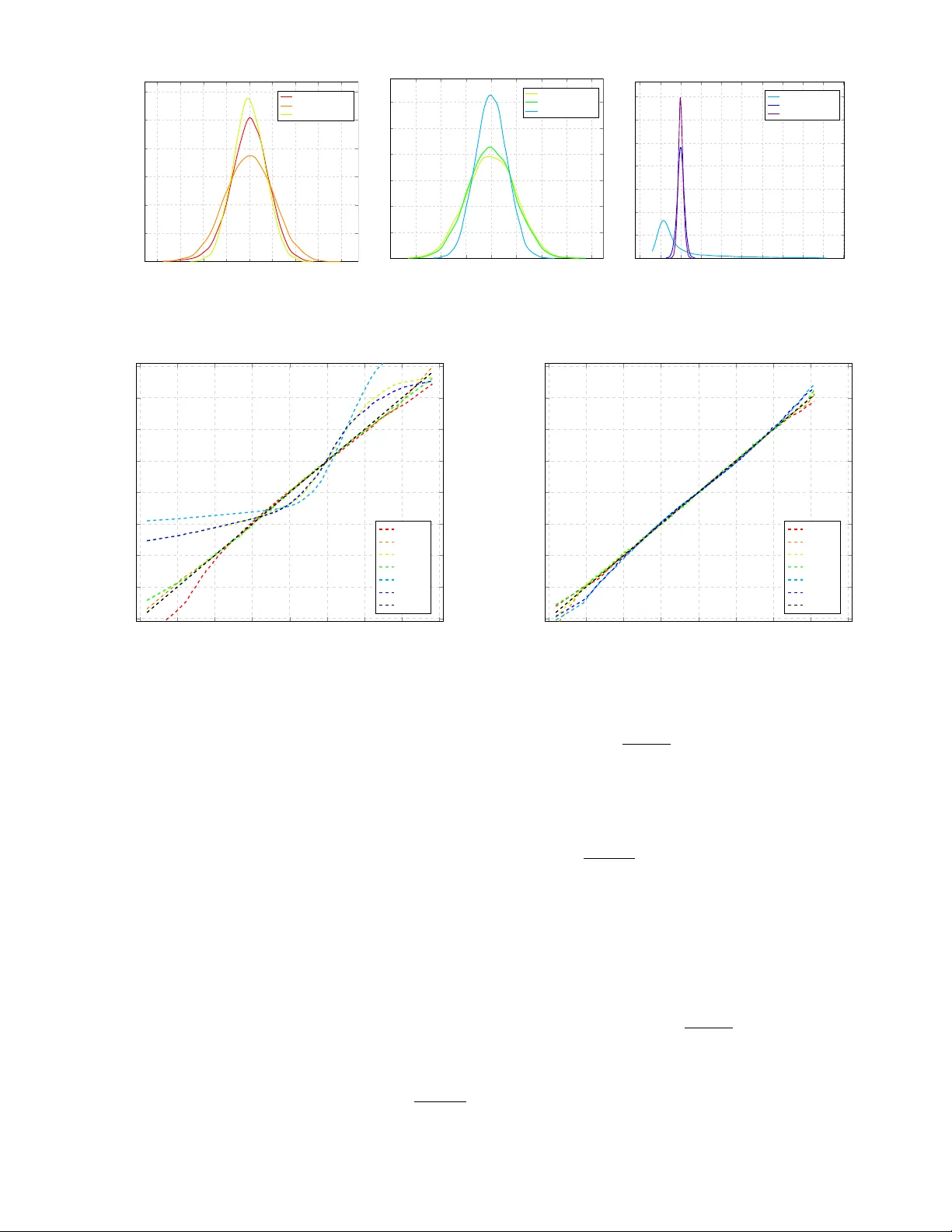
Proof of Concept: Local TX Real-T ime Phase Calibration in MIMO Systems Carl Collmann, Ahmad Nimr , Gerhard Fettweis V odafone Chair Mobile Communications Systems, T echnische Univ ersit ¨ at Dresden, Germany { carl.collmann, ahmad.nimr, gerhard.fettweis } @tu-dresden.de Abstract —Channel measurements in multiple-input multiple- output (MIMO) systems hinge on precise synchr onization. While methods for time and fr equency synchronization ar e well es- tablished, maintaining real-time phase coherence remains an open r equirement f or many MIMO systems. Phase coherence in MIMO systems is crucial for beamforming in digital arrays and enables precise parameter estimates such as Angle-of- Arrival/Departur e. This work presents and validates a simple local r eal-time phase calibration method for a digital array . W e compare two different approaches, instantaneous and smoothed calibration, to determine the optimal interval between synchro- nization procedures. T o quantitatively assess calibration perfor - mance, we use two metrics: the average beamforming power loss and the root mean square (RMS) cycle-to-cycle jitter . Our results indicate that both appr oaches f or phase calibration are effective and yield RMS of jitter in the 2 . 1 ps to 124 fs range for different software-defined radio (SDR) models. This level of pre- cision enables coherent transmission on commonly available SDR platforms, allowing in vestigation on advanced MIMO techniques and transmit beamforming in practical testbeds. Index T erms —software-defined radio, multiple-input multiple- output, radio frequency transceiver I . I N T R O DU C T I O N Phase noise in multiple-input multiple-output (MIMO) com- munication systems significantly degrades data throughput [1] and in the context of joint communication and sensing (JCnS) limits the accuracy of parameter estimates [2]. The compensation of phase noise at the recei ver side is well established. F or e xample the 3GPP standard [3] of fers the phase tracking reference signal (PT -RS) to compensate for the constant phase error (CPE) induced by phase noise. Howe ver to enable transmit beamforming in a digital array , coherence between radio frequency (RF) chains feeding the transmitting antenna array has to be assured. There are sev eral known calibration approaches in the literature, each with limitations. Reciprocity calibration Over - the-Air (O T A) with distributed sensor nodes such as [4] and [5] lacks a shared phase reference, making it unsuitable for coherent combination of the signals from multiple transmitters. In [6] a reciprocity calibration OT A scheme is employed where both transmit and recei ve arrays are connected to a common measurement de vice. This wired connection requires the transmitter and receiv er to be co-located, making the approach unsuitable for mobile communication scenarios. The authors in [7] present OT A reciprocity calibration in MIMO systems, where all distributed radio units are connected to a central controller that performs synchronization by pre-coding TX Controller DUC D/A LP RF DUC D/A LP RF DDC A/D LP RF TX 1 TX M . . . . . . . . . . . . . . . . . . . . . x [ n ] x BB x PB ,m s m y [ n ] y BB y PB r Reference Fig. 1. Setup for phase calibration of TX array , comparison to reference. with phase estimates. A limitation in this work is that the radio units ha ve no method of compensating the local oscillator (LO) phase drifts internally , which imposes a significant o verhead on the OT A calibration. Compounding these challenges, the often neglected residual transmit side calibration errors, can substantially degrade achiev able MIMO throughput [8]. In this work, we address these limitations by proposing and validating a simple, local method for real-time phase calibra- tion of transmit RF chains. Our approach uses a dedicated ref- erence RF chain at the transmitter to recei ve calibration signals (PT -RS) from each transmit chain in a time-division multiple access (TDMA) scheme. The transmit-controller estimates the phase of each chain relative to this reference and applies precoding to achieve coherent transmission in passband. The calibration procedure is performed in periodic intervals to continuously track LO drift, to directly address the transmit side phase impairments as highlighted in [8]. The paper is org anized as follo ws. Section II introduces the system model for local transmitter calibration and modeling of phase noise processes for voltage-controlled oscillator (VCO) and phase-locked loop (PLL). Section III presents measure- ment results and v alidates the calibration approaches. Section IV explores the effect of different calibration interv als and their impact on the achiev able beamforming gain. Finally , the paper is concluded in section V with key results. I I . S Y S T E M M O D E L A. Local Calibration of TX Array Our objective is to calibrate the phase of each element in a transmitting digital antenna array with M elements, as illustrated in Fig. 1. T o achieve this objecti ve, the phases of the transmitting chains must be compared to a common reference. Because the transmitting chains and reference RF chain are co- · · · · · · · · · · · · t syn t dm t obs time t Sync. Preamble Data/Meas. Signal Sync. Preamble TX 1 TX M TX 1 TX M Fig. 2. Phase calibration scheme, periodic transmission of synchronization preamble, observed signal at transmitter reference. located, we assume a common trigger signal (e.g., 1-pulse-per- second) to align the sampling clocks and a common 10 MHz reference are av ailable. While the sampling clocks are con- sidered as ideal, the synthesized carrier signals exhibit phase noise and corresponding drift. Further impairments considered are the phase responses of RF chain components and their respectiv e RF front ends. As shown in Fig. 2, each TX chain transmits a synchro- nization signal x [ n ] of length N in TDMA before the data or measurement signal. The band-limited baseband signal after D/A con version and lo w-pass filtering is denoted x BB ( t ) , defined ov er t ∈ [0 , N T s ] . After up-con version, the bandpass signal for chain m becomes x BP ,m ( t ) = x BB ( t ) e j (2 πf c ,m t + θ OS ,m ( t )) . (1) The synthesized carrier frequency f c ,m is v ariable per chain to model a residual frequency of fset. This small residual carrier frequency of fset (CFO) models a linear phase shift ov er time, distinct from oscillator phase noise. The term θ OS ,m ( t ) refers to the time-dependent phase of the oscillator signal for RF chain m . Then the transmitted signal at RF chain m in TDMA is s TX ,m ( t ) = x BP ,m ( t − mN T s ) e j θ RF ,m (2) The term θ RF ,m represents a constant phase shift specific to chain m . This shift arises from the cumulative phase response of amplifiers, switches, splitters, filters, and other front-end components. As illustrated in Fig. 2, the synchronization preamble has duration t syn = M N T s and is repeated every t obs seconds to obtain phase observations for each chain periodically . The locally recei ved signal at the reference RF chain is the sum of the transmit signals r TX ( t ) = M X m =1 s TX ,m ( t ) . (3) Down-con verting using the reference chain’ s local oscillator at frequency f c yields the baseband receiv ed signal y BB ( t ) = r TX ( t ) e − j 2 πf c t . (4) Note that the receiv ed signal gain is neglected, assuming it is compensated by an automatic g ain control (A GC). Furthermore, the phase shift of the RF components at the reference chain is neglected, as it will induce an identical phase shift for all s TX ,m ( t ) and only the relativ e phase relation of RF chains are of interest. For simplicity , the phase noise introduced by the oscillator of the reference chain is neglected under the assumption that t syn is suf ficiently short. As a frequency offset are already modeled at the transmitting RF chain, the synthesized carrier frequency at the reference chain is assumed to be ideal. Assuming | x BB ( t ) | 2 = 1 , the system function estimate for chain m is obtained by multiplying the receiv ed baseband signal with the complex conjugate of the transmitted signal and windowing to the appropriate TDMA slot: ˆ h TX ,m ( t ) = y BB ( t ) · x ∗ BB ( t ) · rect " t −  m + N 2  T s N T s # . (5) The time-dependent phase is then found as arg[ ˆ h TX ,m ( t )] . Assuming this phase consists of a constant term with additiv e Gaussian noise, as elaborated on in section II-B, the optimal estimator is the time a verage [9]. A v eraging this phase over the synchronization interval yields the phase estimate ˆ θ m = 1 N T s Z N T s 0 arg[ ˆ h TX ,m ( t )] dt. (6) The transmission controller Fig. 1 then uses these phase estimates to align all M transmitting RF chains. T o achie ve coherent transmission, the baseband data signal transmitted from all chains z [ n ] is pre-compensated with the most recent phase estimate ˜ z m,l [ n ] = z [ n ] · e − j ˆ θ m,l · rect  n − τ TX ,l t dm  , (7) where ˆ θ m,l is the phase estimate for chain m from the l -th calibration interval [ l − 1 , l ] t obs , and τ TX ,l = t syn + t dm / 2 + lt obs centers the data block within the transmission window Fig. 2. Note that the rectangular expression is used to apply the phase estimate to the data signal block (blue element in Fig. 2). Then the corresponding quasi-coherent transmitted pass-band signal is ˜ s l ( t ) = M X m =1 ˜ z m,l ( t ) e j (2 πf c ,m t + θ OS ,m ( t )+ θ RF ,m ) (8) = M X m =1 z ( t ) e j (2 πf c t + θ m ( t ) − ˆ θ m,l ) · rect  t − τ TX ,l t dm  , with θ m ( t ) = 2 π ∆ f m t + θ OS ,m ( t ) + θ RF ,m and ∆ f m = f c ,m − f c . B. Phase Noise Model IEEE defines phase noise as the random fluctuation in the phase of a periodic signal, typically characterized in the frequency domain by its spectral density [10]. In the time domain, this fluctuation manifests as timing error, or jitter . The phase error resulting from the timing error at chain m for an oscillator operating at frequency f c is θ OS ,m ( t ) = 2 π f c α m ( t ) . In the case of a free running VCO, the jitter can be represented by a W iener process [11]. In continuous time, α VCO ( t ) = √ c VCO Z t 0 ξ ( t ′ ) dt ′ , (9) where c VCO is the oscillator constant and ξ ( t ) represents a Gaussian process with unit variance. When this process is sampled at T s to obtain ξ ( iT s ) discrete increments, the jitter can be written as α VCO [ n ] = ( 0 , n = 0 √ c VCO T s P n − 1 i =0 ξ ( iT s ) , n > 0 . (10) Note that to obtain the W iener process, the Gaussian process is scaled with the oscillator constant c VCO . This yields a 1 /f 2 phase noise spectrum with 3 dB bandwidth f 3dB = π f 2 c c VCO . In a PLL, the VCO is placed in a control loop that suppresses long-term drift by comparing its output to a stable reference signal. It is assumed that both reference oscillator and VCO can be modeled as free running oscillators and that the PLL is in locked state. Then the PLL output jitter in discrete time is giv en by [12] α PLL [ n ] =      0 , n = 0 P n − 1 i =0 ( α PLL [ i ] − α REF [ i ]) · ( − 2 π f PLL T s ) + α VCO [ n − 1] , n > 0 . (11) The bandwidth of the PLL is represented by f PLL and c REF refers to the oscillator constant of the reference oscillator . The software-defined radio (SDR) platforms used in our measurements employ PLL’ s locked to a common 10 MHz reference. The model for a PLL can be simplified under the following conditions: 1) the oscillator constant for the reference oscillator is sufficiently high so that during an observation period t obs the condition c VCO >> c REF applies, 2) the PLL bandwidth is sufficiently high f PLL >> f 3dB 3) the process is sampled so that 1 T s > f PLL , 4) the observation time is short t obs < c VCO − 3 c REF c REF 2 π f PLL [12]. Then, the jitter at PLL output can be treated as white noise and described by α PLL [ n ] = α 0 + w [ n ] , where w [ n ] ∼ N (0 , c VCO T s ) is white Gaussian noise. The term α 0 ∼ U (0 , f − 1 c ) refers to a uniformly distributed constant time shift. Compensating this constant of fset is essential for initial phase alignment, while periodic calibration tracks the time-v arying component w [ n ] . In continuous time the phase of RF chain m is θ m ( t ) = 2 π f c α PLL ,m ( t ) . This approximation is validated through measurements in the following section. I I I . M E A S U R E M E N T R E S U LT S A. Measurement Setup Fig. 3 shows the measurement setup used to ev aluate the proposed real-time phase calibration method. The system follows the architecture described in [13]. Each TX RF chain transmits the synchronization signal in a TDMA scheme. The synchronization signal is transmitted ov er cable to receiv er chain RF1 to isolate the phase noise of the transmit chains from channel-induced variations. From this recorded signal, T ABLE I S Y ST E M PA R AM E T E RS M E AS U R E ME N T . Parameter Symbol V alue Carrier frequency f c 3 . 75 GHz Bandwidth B 1 MHz Sample frequency f s 4 MHz TX RF chains M 6 Observations L 10000 Obs. Interv . t obs 100 ms Samples N 2500 TX RF0 TX RF3 D/A D/A TX RF1 TX RF2 D/A D/A τ d , 0 τ d , 1 τ d , 2 τ d , 3 RX RF0 ϕ  k  n d RX RF1 NI LabVIEW RX Con trol le r NI LabVIEW TX Con troller Mein b erg 170 MP meas. sync. RF Signal PPS Signal 10 MHz REF Ethernet ˆ φ 0 , ˆ φ 1 , ˆ φ 2 , ˆ φ 3 Fig. 3. System setup for transceiver with 4 TX and real-time calibration [13]. the RX controller estimates the phases of the transmitting RF chains. These phase estimates are sent to the TX controller on a host PC for precoding to allow for coherent transmission as shown in eq. (7). Measurements were performed on six transmit chains using three different versions of the uni versal software radio periph- eral (USRP) X310 . Ke y parameters for the measurement are giv en in T able I. W ith observ ation interval t obs = 100 ms and L = 10000 observations, the total measurement duration was 0 100 200 300 400 500 600 700 800 900 1 , 000 0 20 40 60 80 100 120 140 160 180 Time [s] Phase ˆ θ m [ deg ] TX 1 - USRP X310 40 MHz TX 2 - USRP X310 40 MHz TX 3 - USRP X310 120 MHz TX 4 - USRP X310 120 MHz TX 5 - USRP X310 160 MHz TX 6 - USRP X310 160 MHz Fig. 4. Estimated phases for 6 transmit chains [14]. 1000 s . Fig. 4 illustrates the estimated phases over time. Sev eral observations can be made from the measurement data [14] sho wn in Fig. 4. During the first 250 s of operation, the phases of TX5 and TX6 (cyan and blue traces) drift by approximately 25 ◦ and 5 ◦ , respectively , despite all chains sharing a common 10 MHz reference. This effect is likely caused by temperature-induced changes in the phase response of the RF frontend during warm up. Other chains such as TX3 and TX4 (lime and green trace) and exhibit negligible drift during the measurement. This is likely due to these chains being already warm from previous measurements when the recording began. These observations highlight the impor- tance of allowing sufficient warm up time of RF components in practical deployments. As demonstrated in the following subsections, the proposed calibration method is suitable for tracking these phase v ariations, enabling coherent transmission despite this temperature induced drift. B. Jitter distribution Analyzing the PDF of the timing jitter provides insight into the effecti veness of the proposed calibration methods. The jitter for chain m at observation interv al l is obtained from the phase estimates as α m,l = ˆ θ m,l 2 π f c . (12) The PDF is estimated using a Gaussian kernel density estimate (KDE) applied to the measured jitter values. T wo calibration approaches are considered: • Instantaneous calibration: precoding with most recent phase estimate as in Eq. (7) • Smoothed calibration: precoding using the av erage of the last 10 phase estimates, 1 10 P 9 k =0 ˆ θ m,l − k , to reduce estimation noise. As a quantitative metric, the root mean square (RMS) cycle- to-cycle jitter is used with definition τ RMS ,m = 1 2 π f c v u u t 1 L − 1 L − 1 X l =0 | ˆ θ m,l +1 − ˆ θ m,l | 2 . (13) Note that this metric is valid only when the phase is suffi- ciently stationary ov er the observation period [15]. Fig. 5, 6, and 7 show the jitter PDF’ s for TX1, TX4 and TX5, illustrating different time-dependent phase responses. T able II summarizes the corresponding RMS jitter values. 1) RF Chains with Ne gligible Drift: TX1 Fig. 5 exhibits negligible drift during the total measurement duration, with a near-Gaussian jitter distribution (red) and RMS value of 1 . 66 ps . Instantaneous calibration (orange) slightly increases the RMS jitter to 2 . 06 ps . This effect occurs because the cal- ibration correction applied in eq. (9) effecti vely differentiates the phase, which amplifies high-frequency noise. The increase is small relative to the uncalibrated jitter , indicating that calibration is not necessary when drift is negligible. Smoothed calibration (lime) reduces the jitter to 1 . 39 ps . T ABLE II R M S C Y C L E - T O - C Y C LE J I T TE R F OR D I FF ER E N T T X . No calib . Inst. calib . Sm. calib . TX1 1 . 66 ps 2 . 06 ps 1 . 39 ps TX2 3 . 03 ps 3 . 20 ps 2 . 15 ps TX3 728 fs 199 fs 134 fs TX4 193 fs 183 fs 124 fs TX5 7 . 78 ps 891 fs 632 fs TX6 2 . 99 ps 893 fs 630 fs TX4 Fig. 6 shows lo w intrinsic jitter ( 193 fs RMS). Instanta- neous calibration yields marginal improv ement ( 183 fs RMS), while smoothed calibration achiev es 124 fs RMS. 2) RF Chains with Significant Drift: TX5 Fig. 7 exhibits significant drift, as evident from its PDF without calibration (cyan, 7 . 78 ps RMS). Instantaneous calibration effecti vely compensates this drift, resulting in a Gaussian distribution (blue, 891 fs RMS). Smoothed calibration further reduces jitter to 632 fs RMS (violet), demonstrating the benefit of averaging. After calibration, the RMS jitter is consistent within each USRP v ariant: TX3 and TX4 ( 124 to 134 fs ) and TX5 and TX6 ( 630 to 632 fs ) show excellent agreement. TX1 and TX2 ( 1 . 39 to 2 . 15 ps ) exhibit more variation but remain within the same order of magnitude. C. Quantile-Quantile Plot A quantile-quantile (Q-Q) plot is a graphical method for comparing the similarity of a distribution to the normal distri- bution. In this plot, the quantiles of the ev aluated distribution (typically on the y-axis) are plotted against the quantiles of a normal distrib ution (typically on the x-axis). The distributions are normalized by their standard deviations to allow for even comparison. If a distribution function matches the normal distribution, the Q-Q plot data points fall on a straight line (see Fig. 8 black trace). Fig. 8 shows the Q-Q plot for the estimated phases be- fore calibration. The distributions for TX3, TX5, and TX6 deviate substantially from the reference line, indicating a non- Gaussian PDF. This is consistent with Fig. 4, which sho ws sig- nificant drift for TX5 and TX6 over the measurement duration. From Fig. 7 it can also be seen that the PDF for TX5 (cyan) is not Gaussian and that the phase of this chain drifts during the measurement. For the other RF chains TX1, TX2 and TX4 the distributions are approximately Gaussian. In contrast, TX1, TX2, and TX4 are approximately Gaussian, though TX1 exhibits slight de viation at the tails of its distribution at higher quantiles. After applying the proposed calibration, the Q-Q plot in Fig. 9 shows that all distributions align closely with the normal distribution. This indicates that the residual jitter and corresponding phase errors are Gaussian distributed, which suggests that the calibration has effecti vely whitened the phase noise. A slight deviation at the tails of the distribution ( ± 2 standard deviations) is still visible. Howe ver , this affects only − 8 − 6 − 4 − 2 0 2 4 6 8 0 5 · 10 − 2 0 . 1 0 . 15 0 . 2 0 . 25 0 . 3 Jitter α [ps] Gaussian KDE PDF TX1 no calib. TX1 inst. calib. TX1 sm. calib. Fig. 5. PDF for TX1 before/after calibration − 0 . 8 − 0 . 6 − 0 . 4 − 0 . 2 0 0 . 2 0 . 4 0 . 6 0 . 8 0 0 . 5 1 1 . 5 2 2 . 5 3 Jitter α [ps] Gaussian KDE PDF TX4 no calib. TX4 inst. calib. TX4 sm. calib. Fig. 6. PDF for TX4 before/after calibration − 10 − 5 0 5 10 15 20 25 30 35 40 0 0 . 1 0 . 2 0 . 3 0 . 4 0 . 5 0 . 6 0 . 7 Jitter α [ps] Gaussian KDE PDF TX5 no calib. TX5 inst. calib. TX5 sm. calib. Fig. 7. PDF for TX5 before/after calibration − 4 − 3 − 2 − 1 0 1 2 3 4 − 4 − 3 − 2 − 1 0 1 2 3 4 Quantiles of normal distribution Quantiles of phase distribution TX1 TX2 TX3 TX4 TX5 TX6 ideal Fig. 8. Measured quantiles of phase plotted over quantiles of normal distribution a small fraction of the distribution. W ithin the central 95% of the probability mass, the fit to a normal distribution is decent. I V . S I M U L A T I O N R E S U L T S Numerical simulations are performed to complement the hardware measurements by allowing systematic variation of the observation interval t obs , enabling in vestigation of calibra- tion performance beyond the fixed conditions of the experi- mental setup. A. Effect of Calibration in T ime Domain When continuous calibration is applied, the observation interval t obs has a direct effect on the residual jitter . This section in vestigates this relationship for both free-running VCO and a PLL, with RMS of the cycle-to-cycle jitter τ RMS as defined in eq. (13) as a metric. Ke y simulation parameters are listed in T able III. Fig. 10 shows the RMS of the jitter processes for the uncalibrated and calibrate case, at different observ ation inter- vals. T wo theoretical lower bounds are also shown: √ c VCO t obs − 4 − 3 − 2 − 1 0 1 2 3 4 − 4 − 3 − 2 − 1 0 1 2 3 4 Quantiles of normal distribution Quantiles of phase distribution TX1 TX2 TX3 TX4 TX5 TX6 ideal Fig. 9. Quantiles of phase after calibration plotted over quantiles of normal distribution for the VCO and √ c REF t obs for the PLL, representing the fundamental limits set by oscillator properties. 1) F r ee-Running VCO: F or the uncalibrated VCO (black trace), τ RMS increases with t obs , consistent with the variance scaling σ 2 = c VCO t [12]. Both instantaneous and smoothed calibration (lime and violet traces) achieve the theoretical lower bound √ c VCO t obs across all observ ation intervals, con- firming that the calibration method optimally compensates the VCO phase noise. 2) Phase-Locked-Loop: The uncalibrated PLL (blue trace) exhibits a similar behaviour , with a increase of τ RMS ov er t obs . After calibration, three observations stand out. First, smoothed calibration consistently outperforms the instanta- neous calibration by a slight margin. Second, the calibrated jitter RMS for longer intervals is asymptotically bounded by the reference oscillator limit √ c REF t obs (orange trace). Third, below approximately 10 ms , the jitter reaches a floor and does not improv e with shorter t obs . This howe ver is not due to a limitation on the calibration but innate properties of a PLL. In the transition region between VCO-dominated and 10 − 5 10 − 4 10 − 3 10 − 2 10 − 1 10 0 10 − 16 10 − 15 10 − 14 10 − 13 10 − 12 10 − 11 10 − 10 10 − 9 Obs. Interv. t obs [s] τ RMS [s] PLL sm. PLL calib. REF std. PLL VCO sm. VCO calib. VCO std. VCO 10 − 5 10 − 4 10 − 3 10 − 2 10 − 1 10 0 10 − 16 10 − 15 10 − 14 10 − 13 10 − 12 10 − 11 10 − 10 10 − 9 Obs. In terv. t obs [s] τ RMS [s] PLL sm. PLL calib. REF std. PLL V CO sm. V CO calib. V CO std. V CO 10 − 5 10 − 4 10 − 3 10 − 2 10 − 1 10 0 10 − 16 10 − 15 10 − 14 10 − 13 10 − 12 10 − 11 10 − 10 10 − 9 Obs. In terv. t obs [s] τ RMS [s] PLL sm. PLL calib. REF std. PLL V CO sm. V CO calib. V CO std. V CO Fig. 10. RMS of Cycle-to-cycle jitter for different observation intervals. − 80 − 60 − 40 − 20 0 20 40 60 80 − 12 − 10 − 8 − 6 − 4 − 2 0 Angle [ ° ] Normalized Gain [dB] ideal VCO VCO calib. PLL PLL calib. Fig. 11. Array response under phase impairments with and without periodic calibration 10 − 5 10 − 4 10 − 3 10 − 2 10 − 1 10 0 10 − 7 10 − 6 10 − 5 10 − 4 10 − 3 10 − 2 10 − 1 10 0 10 1 10 2 Obs. Interv. t obs [s] Beamforming loss ¯ p [dB] PLL calib. PLL VCO calib. VCO Fig. 12. A verage beamforming loss in steering direction for different observation intervals reference oscillator-dominated regimes, the PLL jitter variance is bounded by [12] σ 2 = c VCO − 3 c REF 4 π f PLL . (14) For the giv en parameters in T able III this ev aluates to a vari- ance of 7 . 957 × 10 − 28 s 2 , with RMS jitter of 2 . 821 × 10 − 14 s . The smoothed calibration trace in Fig. 10 reaches exactly this value, demonstrating that the proposed method achiev es the fundamental performance bound for PLL’ s. B. Effect of Calibration on Beamforming On the transmit side, coherence of the RF chains in a fully digital array is essential to allow for beamforming. Consequently , significant imperfections in phase calibration of the array will result in a loss in beamforming gain in the desired steering direction. Fig. 11 shows the array response at boresight for arrays affected by VCO and PLL phase impairments, assuming an initial calibration has been performed, with and without sub- sequent periodic calibration. Without periodic calibration, the array subjected to phase noise from a VCO (red trace) shows no coherent beamforming pattern. W ith periodic calibration (orange trace), a clear main lobe emerges. A small of fset from the ideal gain remains, as the VCO jitter over the 100 ms observation interval is still significant. Since the PLL output process does not drift significantly for the considered observation interval, the array response ev en without applying periodic calibration (green trace) is already near ideal. Applying the calibration procedure to compensate the PLL jitter process (blue trace) yields only a small improvement in the side lobes. For the PLL the cases with and without periodic calibration achieve near-optimal beamforming gain. This is because the PLL holds its output phase nearly constant ov er the 100 ms observation interval, exhibiting negligible drift. As a metric to assess the beamforming performance with and without periodic calibration, the av erage beamforming loss in steering direction is considered. This av erage beamforming loss ¯ p is calculated as the difference between ideal gain and T ABLE III S Y ST E M PA R AM E T E RS S I MU L A T I O N . Parameter Symbol V alue Carrier frequency f c 3 . 75 GHz Sample frequency f s 20 MHz TX RF chains M 8 Observations L 1000 Obs. Interv . t obs { 1 ms , . . . , 10 µ s } Samples N 100 Osc. Const. VCO c VCO 1 × 10 − 20 s Osc. Const. REF c REF 1 × 10 − 26 s PLL Bandw . f PLL 1 MHz obtained gain in steering direction and a veraged over steering angles ϕ ∼ U ( − 60 ◦ , 60 ◦ ) . Fig. 12 shows the average beamforming loss for VCO and PLL cases with and without periodic calibration. For the considered array size, a maximum gain of 6 dB can be achiev ed. This value corresponds to the loss observed for the VCO without periodic calibration (black trace) at longer observation intervals. Below an observation interval of ≈ 1 ms , the loss declines. This is due to the observ ation interval being sufficiently short that the VCO cannot drift that far in this time period, allowing the initial calibration to remain partially ef fectiv e. When the VCO jitter is periodically calibrated for (violet trace) but the observ ation interv al is long ( 1 s ), there is no improvement over the case with only initial calibration. This is due to the VCO drifting sufficiently far between calibration times, rendering beamforming ineffecti ve. For all shorter observation interv als, periodic calibration yields a significant improv ement in beamforming loss. In the case of a PLL with only initial calibration (blue trace), the beamforming loss is ne gligibly small meaning that there is no need for periodic calibration with the giv en choice of parameters. Still, periodic calibration (cyan trace) can further reduce this loss by approximately an order of magnitude. For short observ ation intervals below 1 ms the beamforming loss reaches a floor . This corresponds to the fundamental PLL jitter limit as discussed previously and observed also in Fig. 10. V . C O N C L U S I O N Commonly kno wn methods for compensation of phase noise in MIMO systems typically apply phase noise calibration at the receiver . Ho wev er , transmit-side beamforming with large arrays requires real-time phase coherence across all RF chains during transmission. This paper has presented and validated a simple method for real-time phase calibration of fully digital transmit arrays. T wo calibration approaches were compared: instantaneous compensation using the most recent phase estimate, and smoothed compensation using a time average of the last 10 estimates. Measurements on six USRP X310 chains demon- strated that both methods significantly reduce phase drift and jitter . Key results include: • RMS cycle-to-c ycle jitter reduced to as low as 124 fs for PLL’ s, with smoothed calibration consistently outper- forming instantaneous calibration. • Thermal drift of up to 25 ◦ observed during warm-up period, despite a common 10 MHz reference, highlight- ing the need for calibration ev en with shared reference oscillator . • After calibration, residual phase errors are Gaussian dis- tributed, as confirmed by QQ plot analysis, indicating whitening of the phase noise. • Simulation results showed that the proposed method achiev es the fundamental PLL jitter limit of 2 . 28 × 10 − 14 s for the giv en system parameters and optimal choice of observation interval duration. These results demonstrate that the proposed low-comple xity calibration methods are well-suited for synchronizing SDR- based testbeds and ensuring coherence in MIMO channel measurements. Future work could extend this approach to joint transmitter- receiv er calibration, integrate it with over -the-air reciprocity calibration methods, and in vestigate its performance under mobile conditions where Doppler effects become significant. A C K N O W L E D G M E N T This work was supported by BMBF under the project K OMSENS-6G (16KISK124). R E F E R E N C E S [1] A. Pitarokoilis, S. K. Mohammed, and E. G. Larsson, “Uplink perfor- mance of time-reversal mrc in massive mimo systems subject to phase noise, ” IEEE Tr ansactions on W ireless Communications , vol. 14, no. 2, pp. 711–723, 2015. [2] F . Liu, Y . Cui, C. Masouros, J. Xu, T . X. Han, Y . C. Eldar, and S. Buzzi, “Integrated sensing and communications: T oward dual-functional wire- less networks for 6g and beyond, ” IEEE J ournal on Selected Ar eas in Communications , vol. 40, no. 6, pp. 1728–1767, 2022. [3] E. 3GPP , “5G NR; Physical channels and modulation, ” T echnical Spec- ification (TS) 38.211, 01 2026, v19.2.0. [4] S. Prager, M. S. Haynes, and M. Moghaddam, “W ireless subnanosecond rf synchronization for distributed ultrawideband software-defined radar networks, ” IEEE T ransactions on Micr owave Theory and T echniques , vol. 68, no. 11, pp. 4787–4804, 2020. [5] J. Querol, J. C. Merlano-Duncan, L. Martinez-Marrero, J. Krivochiza, S. Kumar , N. Maturo, A. Camps, S. Chatzinotas, and B. Ottersten, “ A cubesat-ready phase synchronization digital payload for coherent distributed remote sensing missions, ” in 2021 IEEE International Geo- science and Remote Sensing Symposium IGARSS , 2021, pp. 7888–7891. [6] M. Jokinen, O. Kursu, N. T ervo, A. Paerssinen, and M. E. Leinonen, “Over -the-air phase calibration methods for 5g mmw antenna array transceiv ers, ” IEEE Access , vol. 12, pp. 28 057–28 070, 2024. [7] Y . Cao, P . W ang, K. Zheng, X. Liang, D. Liu, M. Lou, J. Jin, Q. W ang, D. W ang, Y . Huang, X. Y ou, and J. W ang, “Experimental performance ev aluation of cell-free massive mimo systems using cots rru with ota reciprocity calibration and phase synchronization, ” IEEE Journal on Selected Areas in Communications , vol. 41, no. 6, pp. 1620–1634, 2023. [8] C. Studer , M. W enk, and A. Burg, “Mimo transmission with residual transmit-rf impairments, ” in 2010 International ITG W orkshop on Smart Antennas (WSA) , 2010, pp. 189–196. [9] S. M. Kay , Fundamentals of statistical signal pr ocessing: estimation theory . USA: Prentice-Hall, Inc., 1993. [10] IEEE, “Ieee standard for jitter and phase noise, ” IEEE Std 2414-2020 , pp. 1–42, 2021. [11] A. Demir , A. Mehrotra, and J. Roycho wdhury , “Phase noise in oscil- lators: a unifying theory and numerical methods for characterization, ” IEEE Tr ansactions on Circuits and Systems I: Fundamental Theory and Applications , vol. 47, no. 5, pp. 655–674, 2000. [12] C. Collmann, B. Banerjee, A. Nimr , and G. Fettweis, “ A practical analysis: Understanding phase noise modelling in time and frequency domain for phase-lock ed loops, ” 2025. [Online]. A vailable: https://arxiv .org/abs/2507.12146 [13] C. Collmann, A. Nimr, and G. Fettweis, “Reliable angle estimation in true-time-delay systems with real-time phase calibration, ” in 2025 IEEE 5th International Symposium on Joint Communications & Sensing (JC&S) , Oulu, Finland, Jan 2025, p. 2. [14] C. Collmann, “Phase measurements for coherent transmission in mimo system with usrp x310, ” 2026. [Online]. A vailable: https://dx.doi.org/10.21227/vnn4-cz93 [15] M. Loehning, “ Analyse und modellierung der effekte von abtast-jitter in analog-digital-wandlern, ” Doctoral Dissertation, TU Dresden, Dresden, 2006.