Machine Learning in Epidemiology

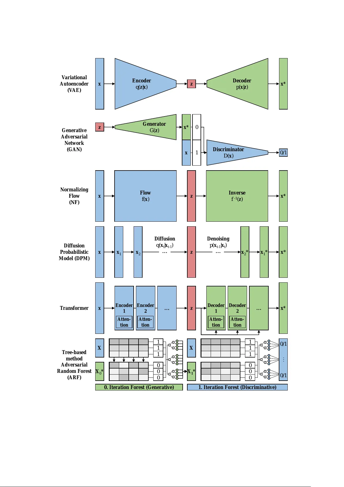
Mac hine Lear ning in Epidemiology Marvin N. W right 1,2,3 , Lukas Burk 1,2 , P egah Golchian 1,2 , Jan Kapar 1,2 , Niklas K oenen 1,2 , and Sophie Hanna Langbein 1,2 1 Leibniz Institute f or Prev ention Resear ch and Epidemiology - BIPS, Br emen, Ger many 2 U niv ersity of Br emen, Germany 3 U niv ersity of Copenhag en, Denmark This is the preprint of the follo wing book chapter: W r ight, M.N., Burk, L., Golchian, P ., Kapar , J., K oenen, N., Langbein, S.H. (2024). Machine Lear ning in Epidemiology . In: Ahrens, W ., Pigeot, I. (eds) Handbook of Epidemiology . Springer , New Y ork, NY , https://doi.org/10.1007/978- 1- 4614- 6625- 3_81- 1 . Abstract In the ag e of digital epidemiology , epidemiologists are f aced by an increasing amount of data of growing comple xity and dimensionality . Machine learning is a set of po w erful tools that can help to analyze such enormous amounts of data. This chapter la ys the methodological f oundations f or successfully appl ying machine learning in epidemiology . It cov ers the principles of super vised and unsupervised lear ning and discusses the most important machine learning methods. Strategies f or model ev aluation and hyperparameter optimization are dev eloped and interpretable machine learning is introduced. All these theoretical parts are accompanied by code e xamples in R , where an e xample dataset on hear t disease is used throughout the chapter . 1 Introduction Machine learning has become an integral part of almost all businesses and scientiﬁc ﬁelds alike, including epidemiology . With the rise of deep learning, machine learning rev olutionized various applications, from image and speech recognition to natural languag e processing. Alongside this h ype, epidemiologists are f aced with an ev er -increasing amount of data of growing comple xity and dimensionality , including data from electronic health records, w earable de vices, social media and g enetics. Machine learning methods are able to eﬃciently anal yze such enormous amounts of data. Thus, in the age of digital epidemiology , machine learning is an essential tool that ev ery moder n epidemiologist should kno w about. One of the major adv antag es of machine learning is that it does not require e xact model speciﬁcations. Instead, one simply indicates whic h v ar iables or f eatures to include, and relies on the mac hine learning method to ﬁnd all the interactions and other impor tant f actors. How ev er, this increased model ﬂe xibility comes at a high computational cost, a loss of inter pretability and the r isk of o verﬁtting, i.e., ﬁtting training data too closely , leading to poor generalization performance and the need f or proper model e valuation. Fur ther , most machine learning methods ha v e to be conﬁgured b y setting so-called hyperparameters, which heavil y inﬂuence per f or mance and thereby ha ve to be chosen carefull y or tested sys tematically . With this book chapter , we aim to giv e epidemiologists the f oundation for successfull y applying machine learning to their research. Notabl y , this does not req uire kno wing all the details of all the diﬀerent mac hine learning methods. Instead, we f ocus on general principles such as supervised lear ning (Sec. 2), model e valuation (Sec. 3) and h yperparameter optimization (Sec. 4). Ne vertheless, we co v er two of the mos t impor tant machine learning methods in Sec. 2. These methods are f ocused on making predictions, which is useful in man y epidemiological tasks, ho we ver , does not help in unders tanding diseases, identifying risk f actors or g enerating synthetic data. In this regard, Sec. 5 introduces the basics of inter pretable machine learning and Sec. 6 cov ers unsuper vised learning and generativ e modeling. Throughout the chapter , we use an e xample dataset on hear t disease and sho w how to appl y the co vered methods in R using the mlr3 frame w ork (Lang et al, 2019). 1 Heart Disease Data Example The heart disease data (Janosi et al, 1988) are av ailable from OpenML (V anschoren et al, 2013). The labeled dataset contains 𝑛 = 270 instances of patients with 𝑝 = 13 features. The features include a patient’ s age ( age ), results of a thallium s tress test ( thal ) and f our types of ches t pain ( chest pain ), among others. W e aim to predict whether the tar get heart disease 𝑦 ∈ { 1 , 2 } is absent (1) or present (2). Since 𝑦 is categorical with tw o classes, it is a binary classiﬁcation task. For details on the dataset, preprocessing, software and code e xamples, w e ref er to the appendix, our GitHub page https://github.com/bips- hb/epi- handbook- ml , and the mlr3 book (Bischl et al, 2024). 2 Supervised Learning Supervised lear ning ref ers to lear ning a functional relationship, or model, ˆ 𝑓 : 𝑋 → 𝑌 betw een a set of 𝑝 f eatures 𝒙 ∈ 𝑋 ⊆ R 𝑝 and a targ et 𝑦 ∈ 𝑌 ⊆ R from data D = { ( 𝒙 𝑖 , 𝑦 𝑖 ) } 𝑛 𝑖 = 1 with 𝑛 ∈ N instances. It is uniq uely c haracterized b y the use of labeled training data f or lear ning the underl ying relationship 𝑓 : 𝑋 → 𝑌 . W e refer to labeled data if both features and targets are obser v ed. The model ˆ 𝑓 is then used to make predictions for the target of new data ˆ 𝑦 = ˆ 𝑓 ( 𝒙 ) , where the features but not the targets are av ailable. An ex ample prediction task f or the ﬁeld of epidemiology ma y be predicting the risk of a speciﬁc disease, based on genetic and lif estyle f eatures. It is important to note that the term model is used for man y diﬀerent concepts in science, whic h may lead to confusion. In this chapter , the term model is used to ref er only to the functional relationship ˆ 𝑓 betw een 𝒙 and 𝑦 . The algorithm that is used to ﬁnd the model is ter med inducer or lear ner . Generally , supervised learning with a continuous tar get 𝑦 ∈ R is ref er red to as a r egr ession task. A classiﬁcation task is presented, when 𝑦 is categorical, i.e., 𝑦 ∈ { 1 , . . . , 𝐶 } , where 𝐶 ∈ N is the number of classes. In this case, the prediction can either be categor ical, i.e., ˆ 𝑦 ∈ { 1 , . . . , 𝐶 } , or probabilistic in nature with ˆ 𝜋 = 𝑃 ( 𝑦 = 𝑐 | 𝒙 ) f or each class 𝑐 ∈ { 1 , . . . , 𝐶 } . For only tw o classes ( 𝐶 = 2), typically a { 0 , 1 } targ et is used, hence it is referred to as binar y classiﬁcation , while 𝐶 > 2 is called multiclass classiﬁcation . For ev aluation purposes, the diﬀerence between the predicted values ˆ 𝑦 and the actual values 𝑦 is usually quantiﬁed in the f orm of a loss function 𝐿 ( ˆ 𝑦 , 𝑦 ) . It measures the per f or mance of a model and the goal is often to minimize this function during training to improv e the model’ s accuracy , for further details see Sec. 3. 2.1 T ree-based Machine Learning Me thods As the name sugges ts, tree-based machine lear ning methods are based on so-called decision trees . Decision trees are used in a v ar iety of contexts apar t from machine learning f or the pur pose of simple, r ule-based decision-making. In g eneral, trees are said to reﬂect the human decision-making process w ell (Gareth et al, 2021). Although decision trees may seem s traightf or ward or e ven trivial, they are indeed building blocks of po werful learners. The follo wing sections ﬁrst explain classiﬁcation and regression trees (CAR T) – one of the major decision tree algorithms – f ollow ed by so-called ensemble methods, whic h combine sev eral decision trees. Finall y , w e give an e xample of a decision tree on the heart disease data introduced in Sec. 1. 2.1.1 Classiﬁcation and Regr ession T rees Classiﬁcation and regression trees (CAR T) are constr ucted b y recursivel y par titioning the instances of the training dataset into subgroups. An e xample is sho wn in Fig. 1 (a), sho wing a tree of sev en nodes, including a root node at the top of the tree, f our leaf nodes at the bottom and two internal nodes in between. The algorithm star ts at the root node with the full training data and ﬁnds the best split with regard to a loss function. This results in two child nodes, which are then recursiv ely split according to the same scheme, until a s topping cr iterion is reached. In the resulting terminal nodes, or leav es, a prediction is made based on a probability estimate or majority vote. Fig. 1 (b) illustrates the corresponding par titioning of two e xemplary f eatures, where the shaded regions represent the binar y predictions. More formally , the space 𝑋 is divided into 𝑀 disjoint regions 𝑅 𝑚 with 𝑚 = 1 , . . . , 𝑀 , cor responding to the leav es of the tree. In each region, a simple prediction model is ﬁtted. In CAR T , a constant prediction ˆ 𝑦 𝑚 is used, i.e., f or ev ery instance in a par ticular region 𝒙 ∈ 𝑅 𝑚 , the same prediction ˆ 𝑦 𝑚 is made. With this and Θ = { ( 𝑅 𝑚 , ˆ 𝑦 𝑚 ) } 𝑀 𝑚 = 1 , a tree model ˆ 𝑓 tree can be deﬁned as ˆ 𝑓 tree ( 𝒙 ; Θ ) = 𝑀  𝑚 = 1 ˆ 𝑦 𝑚 1 ( 𝒙 ∈ 𝑅 𝑚 ) , 2 ST_depression < 1.7 ST_depression < 0.85 serum_cholesterol < 224 absent 0.44 100% absent 0.33 75% absent 0.26 53% absent 0.49 23% absent 0.25 7% present 0.61 15% present 0.79 25% yes no (a) Decision tree with 2 f eatures. 200 300 400 500 0 2 4 6 ST_depression serum_cholesterol hear t_disease absent present (b) Partition plot. Figure 1: (a) Decision tree of the hear t disease dataset using only the features ST depression and serum cholesterol . (b) The corresponding par tition plot. The points are the instances/patients, and the shaded areas denote the model predictions. where 1 ( · ) is the indicator function and Θ is ﬁtted by minimizing ˆ Θ = arg min Θ 𝑀  𝑚 = 1  𝑖 : 𝒙 𝑖 ∈ 𝑅 𝑚 𝐿  ˆ 𝑦 𝑚 , 𝑦 𝑖  . That is, ˆ Θ is chosen such that the targ et values of instances that f all into a region 𝑅 𝑚 are close to the prediction ˆ 𝑦 𝑚 of the region, which is ev aluated by a loss function 𝐿 . The optimization problem can be broken do wn into two components – ﬁnding the constants ˆ 𝑦 𝑚 and ﬁnding the regions 𝑅 𝑚 , which, ho we ver , depend on each other . Finding the constant ˆ 𝑦 𝑚 giv en a region 𝑅 𝑚 can be speciﬁed by the input task. In a regression task, the constant is chosen as the arithmetic mean ov er all 𝑦 𝑖 corresponding to the 𝑛 𝑚 data instances f alling in 𝑅 𝑚 . In contrast, f or a classiﬁcation task, the majority class is used. Let 𝑝 𝑚 𝑘 = 1 𝑛 𝑚 Í 𝑖 : 𝒙 𝑖 ∈ 𝑅 𝑚 1 ( 𝑦 𝑖 = 𝑘 ) be the propor tion of instances of class 𝑘 in 𝑅 𝑚 , then, ˆ 𝑦 𝑚 = arg max 𝑘 𝑝 𝑚 𝑘 . Sev eral extensions ha v e been proposed, e.g., f or survival tasks, one could estimate the survival function with the Kaplan-Meier es timator in each leaf separately (Hothorn et al, 2004). T o ﬁnd the regions 𝑅 𝑚 , the algorithm builds the tree using recursiv e binary par titioning or splitting. It starts at the root of the tree with all data and then chooses the best split into tw o par titions locall y at each node. This splitting procedure follo ws the tree structure and does not consider the ov erall best split. Thus, it is a so-called top-do wn g reedy approach. For a continuous or ordinal f eature 𝒙 𝑗 , the regions are divided by the split point 𝑠 ∈ R , such that instances with a f eature value smaller or equal 𝑠 are assigned to the ﬁrst, or left, child node and the remaining instances to the right child node: 𝑅 left ( 𝑗 , 𝑠 ) =  𝒙 | 𝒙 𝑗 ≤ 𝑠  and 𝑅 right ( 𝑗 , 𝑠 ) =  𝒙 | 𝒙 𝑗 > 𝑠  . The best split is found where, in both child nodes, the predicted target is close to the tr ue targ et. T o this end, w e ﬁnd the best pair ( 𝑗 , 𝑠 ) for the split that minimizes the sum of the loss functions in the tw o child nodes: arg min 𝑗 , 𝑠 ©  «  𝑖 : 𝒙 𝑖 ∈ 𝑅 left ( 𝑗 , 𝑠 ) 𝐿  ˆ 𝑦 left , 𝑦 𝑖  +  𝑖 : 𝒙 𝑖 ∈ 𝑅 right ( 𝑗 , 𝑠 ) 𝐿  ˆ 𝑦 right , 𝑦 𝑖  ª ® ¬ . For a categor ical feature 𝒙 𝑗 , we can assign a subset 𝑆 of its categor ies to the left child node and the remaining categories to the r ight child node: 𝑅 left ( 𝑗 , 𝑆 ) =  𝒙   𝒙 𝑗 ∈ 𝑆  and 𝑅 right ( 𝑗 , 𝑆 ) =  𝒙   𝒙 𝑗 ∉ 𝑆  . Note that w e search f or the best split 𝑠 or 𝑆 f or all features 𝒙 𝑗 simultaneously . 3 Depending on the task, diﬀerent loss functions are chosen. For regression tasks, f or instance, the mean squared error (MSE) is often utilized, whereas for classiﬁcation tasks measures lik e cross-entropy or Gini coeﬃcient are pref er red. In pr inciple and depending on the implementation, one could use any ev aluation metr ic; see Sec. 3, where ev aluation metr ics are discussed more generall y and in more detail. In the context of decision trees, the concept of empirical risk or loss minimization is often used interchang eably with the concept of impurity reduction. For e xample, f or a regression tree, minimizing MSE loss is equivalent to maximizing impurity reduction when the impurity is measured by the empirical variance. In theory , the descr ibed algorithm could be continued until no fur ther split is possible. Intuitivel y , the deeper the tree, the more detailed the data are split into subsets. In the e xtreme case, each leaf contains only a single instance and the tree perfectl y predicts the training data. Ho w e v er, in this case, the tree is probabl y ﬁtted too w ell to the training data and f or unseen data, the model could fail. In other words, the model o v erﬁtted (see Sec. 3). Useful in the conte xt of o verﬁtting is the follo wing perspectiv e: Analogous to the abov e deﬁnition of a tree model ˆ 𝑓 tree , a tree can also be represented via the sequence of splits, denoted b y 𝑇 . This intuitivel y allow s for the deﬁnition of subtrees, which only contain a subset of splits until a certain iteration step, i.e., up to a cer tain tree depth. There are sev eral techniques to a void o verﬁtting in trees. Firs t, one typically deﬁnes a stopping criter ion, such as a predeﬁned minimum number of instances in a node or a maximum tree depth. Another option in vol ves growing the tree as long as each split’ s reduction in the loss ex ceeds a predeﬁned threshold. How ev er, while this might perform better than a simple stopping criter ion, it might still not result in an optimal tree due to the greedy nature of the algorithm. This is because a rather non-informativ e split could lead to a better split later on in the tree, i.e., a split that further reduces the loss. For this reason, the usual approach is to ﬁrs t grow a deep tree until a s topping criter ion is reached and then prune the tree, i.e., cut back the lea v es. In cost-complexity pruning , or also called w eakest link pruning , we want to ﬁnd a tree with a good trade-oﬀ betw een high prediction perf or mance and lo w model complexity . For a giv en tree 𝑇 , the tree comple xity can be measured b y the number of leav es | 𝑇 | , since more comple x trees are deeper or wider , cor responding to a higher number of leaf nodes. Prediction performance can be measured by the loss function 𝐿 𝑚 ( 𝑇 ) = Í 𝑖 : 𝒙 𝑖 ∈ 𝑅 𝑚 𝐿  ˆ 𝑦 𝑚 , 𝑦 𝑖  of a tree 𝑇 in the leaf 𝑚 = 1 , . . . , | 𝑇 | , where a lo wer loss indicates a higher prediction per f or mance. The cost comple xity function for a giv en tree 𝑇 is given as 𝐶 𝛼 ( 𝑇 ) = | 𝑇 |  𝑚 = 1 𝑛 𝑚 𝐿 𝑚 ( 𝑇 ) + 𝛼 | 𝑇 | , where 𝑛 𝑚 is the number of instances in leaf 𝑚 and 𝛼 ≥ 0 is a predeﬁned complexity parameter, which adjusts the trade-oﬀ betw een prediction per f or mance and model comple xity . In cost comple xity pruning, we obtain the optimal subtree 𝑇 𝛼 ⊆ 𝑇 among all possible subtrees by minimizing 𝐶 𝛼 . Large 𝛼 values indicate smaller trees and 𝛼 = 0 ref ers to the unpruned tree 𝑇 0 = 𝑇 . W e obtain the best 𝛼 b y , for ins tance, cross-validation (Sec. 3) and take the subtree 𝑇 𝛼 that minimizes the cross-validation error . The beauty of decision trees is that they are intuitive and easy to inter pret. Y et, compared to other more sophisticated machine learning models, their prediction performance is often rather poor . Decision trees suﬀer from high variance, i.e., if we randoml y sample the training dataset and ﬁt a decision tree to each sample, we could get very diﬀerent results. The good new s is that if we combine man y trees on such samples, the performance impro ves a lot. W e will present some methods in the f ollowing that use this idea. 2.1.2 Bagging and Boosting T o ov ercome the high variance of simple lear ners such as decision trees, ensemble methods combine many of such learners into a more po w er ful one. The simple lear ners in an ensemble are also called weak learners since the y w ould lead to mediocre per f or mance on their own. The two mos t popular ensemble methods for decision trees are bagging and boosting , which will be described in the f ollowing. Bootstrap aggregating (bagging) builds multiple models on bootstrapped datasets and aggregates the predictions of those models. The idea of the bootstrap stems from the f ollo wing: If 𝑍 1 , . . . , 𝑍 𝐵 are 𝐵 independent and identically distributed random variables with variance 𝜎 2 , then the variance of the mean ¯ 𝑍 is 𝜎 2 / 𝐵 . Analogously , if w e had man y independent training samples from a population and av eraged the resulting prediction models, w e w ould reduce the variance compared to only using one training sample. Since it is challenging and sometimes impossible to obtain multiple independent training samples, the idea of bootstrapping is to tak e repeated samples (with replacement) from the single training dataset we ha ve. See Sec. 3.2.3 for more details on boots trapping. For bagging, ﬁrst 𝐵 diﬀerent bootstrap samples are generated from the training data and a prediction model, e.g., a decision tree, is ﬁtted on each of the bootstrap samples. Let ˆ 𝑓 𝑏 tree ( 𝒙 ) be the prediction of the decision tree ﬁtted on 4 the 𝑏 th bootstrap sample. Then the bagg ed prediction is deﬁned as ˆ 𝑓 bag ( 𝒙 ) = 1 𝐵 𝐵  𝑏 = 1 ˆ 𝑓 𝑏 tree ( 𝒙 ) . For a classiﬁcation task, one w ould, f or e xample, take the majority vote among all the 𝐵 tree predictions. In contrast to single decision trees, the trees are typically grown deep, f or each tree to ha ve a high v ar iance but lo w bias. Since av eraging the trees reduces the v ar iance, no additional pruning is required. The parameter 𝐵 can be chosen suﬃcientl y large since it does not lead to o verﬁtting. A crucial advantag e of bagging is that, because of sampling with replacement, on av erage onl y 1 − e xp ( − 1 ) ≈ 2 / 3 of the instances are used for model ﬁtting on each bootstrap sample. The remaining 1/3 of instances are called out-of-bag (OOB). OOB instances are very useful when ev aluating the generalization error , which is described in more detail in Sec. 3.2.3. Ho we v er, compared to a single tree, the impro vement in prediction accuracy comes at the cost of interpretability (see Sec. 5). Another disadvantag e of bagging is that the trees grown on diﬀerent boots trap samples may still be quite similar , i.e., highly correlated, and consequentl y the eﬀect of larg e variance reduction may v anish. Similar trees are often created when one or multiple strong features are present because they would be used f or splits close to the root node in e v er y tree. Mathematically speaking, if the random v ariables 𝑍 1 , . . . , 𝑍 𝐵 are identically distributed but not necessar il y independent, the variance of their mean ¯ 𝑍 is 𝜌 𝜎 2 + 1 − 𝜌 𝐵 𝜎 2 , where 𝜌 is the positiv e pairwise cor relation. For 𝐵 → ∞ , the v ariance reduces to the ﬁrst term 𝜌 𝜎 2 . Theref ore, the v ar iance can be reduced, b y reducing 𝜌 , which leads to the idea of random f orests. Random f orests (Breiman, 2001) impro ve bagging by decorr elating the trees, i.e., reducing the pair wise correlation 𝜌 and thereby the v ar iance of the resulting ensemble. The method extends bagging b y consider ing only a randomly sampled subset of size 𝑞 ≤ 𝑝 of all 𝑝 f eatures for each split in a tree. T ypical values f or 𝑞 are 𝑞 ≈ 𝑝 / 3 or 𝑞 ≈ √ 𝑝 . The problem of having a f ew s trong features described abov e is circum v ented by this approach, since on a verag e it is onl y considered f or ( 𝑝 − 𝑞 ) / 𝑝 splits. These hyperparameters, the number of f eatures considered f or splitting at each node 𝑞 and the number of trees 𝐵 , depend on the task but can be tuned (see Sec. 4). Generally , random f orests hav e the advantag e of relativel y easy and fast training and require little tuning. Compared to single decision trees, the performance is often drasticall y impro ved and consequentl y , random fores ts are one of the most popular machine learning methods used in practice. Boosting grow s the trees sequentially on modiﬁed datasets, in contrast to the abo ve methods, which gro w trees in parallel. In boosting, the construction of each successive tree in the ensemble depends on the pre vious tree to use the know ledge g ained from previous f ailures in an iterative learning process. Generally , in boosting, the ensemble consists of a w eighted av erage of the individual trees: ˆ 𝑓 boost ( 𝒙 ) = 𝐵  𝑏 = 1 𝜔 𝑏 ˆ 𝑓 𝑏 tree ( 𝒙 ) , where 𝜔 𝑏 are the w eights and each tree ˆ 𝑓 𝑏 tree ( 𝒙 ) depends on the previous tree ˆ 𝑓 𝑏 − 1 tree ( 𝒙 ) . A daBoost , as introduced b y Freund and Schapire (1997), uses s tumps as w eak lear ners, i.e., trees with onl y one split. In the ﬁrst s tep, a stump is ﬁtted to the or iginal training dataset. Second, it is assessed f or each instance whether it is correctly classiﬁed by the stump. In the ne xt step, weights are assigned to all instances, whereby misclassiﬁed instances are assigned higher weights, while correctly classiﬁed instances are assigned lo wer w eights. Then, another stump is ﬁtted to the weighted dataset. By that, the second stump f ocuses on cor recting the er rors of the ﬁrst stump. The algorithm proceeds iterativel y , where each stump uses the w eights obtained from the previous iteration. T o obtain a ﬁnal prediction, a weighted a verag e of the individual stumps ’ predictions is calculated, where each stump is weighed depending on its perf ormance. A daBoost can be easily extended to other tasks such as regression and the use of deeper trees than just stumps. Gradient boosting (Fr iedman, 2001) w orks in a similar iterative manner , but is based on the par tial der ivativ e, or gradient, of the loss function. For 𝐿 2 loss, the algor ithm starts by ﬁtting a single, typically not very deep, decision tree to the training data, obtaining a prediction ˆ 𝑓 1 tree ( 𝒙 ) . Second, the residuals 𝑦 − ˆ 𝑓 1 tree ( 𝒙 ) of this tree are calculated and used as the target to ﬁt a second tree with prediction ˆ 𝑓 2 tree ( 𝒙 ) . The algorithm proceeds iterativel y f or 𝑏 = 1 , . . ., 𝐵 , where each tree is ﬁtted to the residuals of the previous tree. Thereb y , the algorithm puts its focus gradually on those parts, where the previous trees did not perform well, i.e., where the loss w as large. Similarl y to A daBoost, the ﬁnal prediction is a weighted a verag e of the individual trees. How ev er, f or gradient boosting, the w eights decrease in each iteration b y a learning rat e , which is a h yperparameter that can be tuned. Note that the negativ e gradient of the 𝐿 2 loss is proportional to the residual v ector . Gradient boosting can be generalized to other (diﬀerentiable) loss functions b y using the gradient of the negativ e loss function instead of the residuals. A popular variant of gradient boosting is e xtreme gradient boosting (XGBoost) (Chen and Guestrin, 2016). It e xtends g radient boosting b y further regular ization, e.g., by introducing an additional regular ization term and 5 thal = normal chest_pain = typical angina,atypical angina,non−anginal pain num_major_vessels < 1 num_major_vessels < 1 exer cise_induced_angina = no age >= 51 absent 0.44 100% absent 0.22 56% absent 0.10 37% absent 0.45 19% absent 0.19 11% present 0.85 7% present 0.74 44% present 0.53 20% absent 0.31 11% absent 0.12 6% present 0.58 4% present 0.79 9% present 0.91 24% yes no Figure 2: A decision tree ﬁtted on the hear t disease dataset, visualized with the rpart.plot packag e. It predicts whether hear t disease is present or absent in a patient, based on the f eatures in the dataset, e.g., the results of a thallium stress test ( thal ). Each node contains the follo wing inf or mation: 1) absent/present prediction, 2) propor tion of patients with present hear t disease, 3) size of the node as percentag e of total sample size. The splitting criter ia are denoted belo w the nodes. If the cr iteria apply , w e follo w the left path, other wise the right path. shrinkage of tree weights, and column f eature subsampling similar to random fores ts. XGBoost is computationally fas t and often delivers s tate-of-the-art per f or mance. As a result, it is as popular as random f orests. 2.1.3 Data Example Man y software implementations are a vailable f or building decision trees. In R , w e use the rpart packag e to ﬁt a decision tree to the heart disease data descr ibed in Sec. 1. In Fig. 2, w e sho w the resulting tree. library(rpart) library(rpart.plot) tree <- rpart(heart_disease ˜ ., heart) rpart.plot(tree) Assume a doctor na ¨ ıv ely wants to predict whether to diagnose a ne w patient with hear t disease on the basis of this tree. The doctor w ould then ﬁrst per f or m a thallium stress test. If, f or e xample, the results are not nor mal (right path), the next s tep is to check whether the number of major v essels colored by ﬂuoroscop y is less than one. If that is not the case (right path), the doctor would diagnose a heart disease. As described in the algor ithm abo ve, regions are sequentially divided into smaller regions. This is made apparent by the inf ormation in the nodes. The root node in Fig. 2, for e xample, contains the f ollo wing information: absent, 0.44, 100%. This means that this node contains 100% of the training data with a prev alence of 44%. Since this is the minority , e very ne w ins tance in this node w ould be classiﬁed as absent. The c hild node to the left contains all patients with a nor mal thallium stress test, which amounts to 56% of the training data with a prev alence of 22%. The remaining 44% of the training data, i.e., those with a non-nor mal thallium stress test, are in the r ight child node, where heart disease is present for 74% of patients. Further down in the tree, the nodes become smaller but impro ve in purity , i.e., contain mostl y patients with or without hear t disease. 6 cp X−v al Relativ e Error 0.4 0.6 0.8 1.0 1.2 Inf 0.16 0.052 0.031 0.019 0.014 0.012 0.011 1 2 4 6 8 11 13 16 siz e of tree Tree size Complexity parameter (cp) Prediction error Figure 3: A visual representation of the cross-validation results of the cos t-complexity pruning. The 𝑥 -axis show s the complexity parameter cp . At the top, the number of leaf nodes cor responding to each comple xity parameter is denoted. The 𝑦 -axis represents a prediction er ror measure, based on cross-validation. The low est error is reached at cp of 0.031. Figure created with the rpart packag e and slightly modiﬁed. T o see if w e can improv e upon the tree abo ve, w e no w ﬁt a deeper tree and perf or m cost-comple xity pruning. A deeper tree can be created b y reducing the minimum number of instances in a node to perf or m splitting: tree_deep <- rpart(heart_disease ˜ ., heart, control = rpart.control(minsplit = 2)) In our e xample, this results in a tree of size (number of lea v es) 16. W e can plot an estimate of the generalization error (based on cross-validation) agains t the tree size by plotcp(tree_deep) which outputs Fig. 3. W e observe that the optimal tree has six leav es, which corresponds to a comple xity parameter (denoted as 𝛼 before) cp of 0.031. Hence, we prune the tree by pruned_tree <- prune(tree_deep, cp = 0.031) which results in a tree as in F ig. 2 where w e prune back b y cutting the last split at age ≥ 51. 2.2 Artiﬁcial Neural N etw orks Artiﬁcial neural networks, also known just as neur al netw orks , are the fundamental component of the machine learning subﬁeld of deep lear ning (LeCun et al, 2015; Goodf ellow et al, 2016). Neural networks are c haracter ized b y an e xtraordinar ily ﬂexible and parameter -rich transf or mation. This enables them to lear n highl y complex and non-linear functional relationships between f eatures and targ et variables. Ho we ver , due to the often extremel y high number of model parameters, a sophisticated optimization procedure and regular ization techniques are essential to achie ve good perf ormance on the data used for training as w ell as to generalize on unseen data, i.e., prev enting o verﬁtting. In the follo wing sections, we discuss the possible architectures of neural networks and how their ﬂe xibility is achiev ed. In addition, we e xplore the training and regularization process of these models and conclude with an e xample of constructing and training a neural network in R using the hear t disease dataset. 7 x 1 x 2 x 3 x p . . . . . . . . . . . . . . . . . . . . . ˆ y Input lay er ˆ f 1 Hidden lay ers ˆ f 2 , . . . , ˆ f 6 Output lay er ˆ f 7 F eatures Mo del output b (4) x (4) 1 x (4) 2 x (4) p 4 P P P x (5) 1 x (5) 2 x (5) p 5 . . . . . . . . . σ 4 σ 4 σ 4 Hidden lay er ˆ f 4 σ 4  W (4) T x (4) + b (4)  = x (5) Figure 4: Model architecture of a sequential neural netw ork with sev en dense lay ers, generating predictions ˆ 𝑦 from the input 𝒙 . On the r ight, the model’ s f our th lay er is magniﬁed, mapping the previous lay er’ s output 𝒙 ( 4 ) to the next lay er’ s input 𝒙 ( 5 ) through an aﬃne transf or mation f ollo w ed b y a non-linear function, denoted as 𝜎 4 . 2.2.1 Arc hitecture In the context of neural netw orks, the basic model is commonly described as an arc hitectur e . This term is appropriate because the user acts as an architect equipped with an extensiv e toolbox of modules and h yperparameters to construct a model tailored to their individual problem. The fundamental building blocks are the layers , which essentially constitute simple parameter ized non-linear transformations. The ke y to the ﬂexibility of neural netw orks is that multiple lay ers ˆ 𝑓 1 , . . . , ˆ 𝑓 𝐾 can be combined as long as their dimensions align, resulting in a highly po werful transf or mation as a model (Goodfello w et al, 2016). In most of the standard cases, the lay ers are ar ranged sequentiall y leading to the follo wing mathematical representation with a single input la y er ˆ 𝑓 1 and output lay er ˆ 𝑓 𝐾 depending on the f eatures and type of target: ˆ 𝑓 NN ( 𝒙 ) = ˆ 𝑓 𝐾 ◦ ˆ 𝑓 𝐾 − 1 ◦ . . . ˆ 𝑓 1 ( 𝒙 ) = ˆ 𝑦 , 𝒙 ∈ R 𝑝 . The la y ers located between a neural netw ork’ s input and output la yer are commonl y referred to as hidden layer s , i.e., the lay ers ˆ 𝑓 2 , . . . , ˆ 𝑓 𝐾 − 1 f or the sequential model ˆ 𝑓 NN deﬁned abo ve. As an example, w e illustrate a sequential architecture with 𝐾 = 7 lay ers in Fig. 4. Although increasingl y comple x types of lay ers ha v e been inv ented in recent y ears, they all more or less rel y on the same basic principles. This is captured b y the earliest and most fundamental la yer type of neural netw ork architecture, known as the dense or fully connected lay er. The lay er’ s name and commonly used visualization, e.g., as sho wn in Fig. 4, hav e signiﬁcantly inﬂuenced the term ”neural networks” and its association with the human brain. A dense la y er connects each output v ar iable of the preceding lay er with ev ery input of the subsequent la y er, thus wea ving a dense net of connections, in which the variables are frequently ref er red to as neurons . In addition, each connection contains a weight to regulate the inﬂuence of the cor responding neuron. The output neurons are then computed as the sum of the w eighted input neurons, f ollow ed by a pointwise non-linear activ ation function . From a mathematical perspectiv e, this lay er type can be descr ibed as an aﬃne transf or mation f ollow ed by a pointwise non-linearity . T o be more precise, f or a la yer ˆ 𝑓 𝑘 : R 𝑑 1 → R 𝑑 2 , the la yer ’ s input 𝒙 ( 𝑘 ) is multiplied b y a w eight matrix 𝑾 ∈ R 𝑑 2 × 𝑑 1 , then shifted b y a v ector 𝒃 ∈ R 𝑑 2 , and afterwards passed to a pointwise non-linear function 𝜎 𝑘 , resulting in the input f or the succeeding lay er 𝒙 ( 𝑘 + 1 ) , i.e., ˆ 𝑓 𝑘  𝒙 ( 𝑘 )  = 𝜎 𝑘  𝑾 𝑇 𝒙 ( 𝑘 ) + 𝒃  = 𝒙 ( 𝑘 + 1 ) . While a dense la yer in a neural network bears a resemblance to a generalized linear model, the terminology used in deep learning can be initially confusing f or people with a statistical back ground. For example, the shift v ector 𝒃 , which is kno wn as the intercept 𝜷 0 in linear regression, is referred to as the bias v ector in the context of neural netw orks, and the statistical link function 𝜎 (not to be confused with the s tandard deviation) is called the activation function. Moreo v er, the w eights in neural networks are similar to the coeﬃcients 𝜷 in generalized linear models but do not hav e the same inter pretation due to the lay er -wise stacking. Initially , the hyperbolic tang ent was predominantly emplo y ed as activation function. How ev er , with the r ise of deep learning, the rectiﬁed linear unit 8 (ReL U) has replaced it almost entirely , allo wing the elimination of unnecessary inf ormation for fur ther f or ward propagation eﬃcientl y . Fig. 5a show s the graphs of three typical pointwise activation functions. The choice of activation function is once ag ain left to the user as a hyperparameter . Aside from the activ ations in the hidden lay ers, the activ ation function in the ﬁnal la yer of a neural network pla ys a cr ucial role. For ex ample, in regression tasks, the activation function should be capable of mapping to an y likel y real-valued number . In contrast, the activ ation should output probabilities ranging between 0 and 1 in classiﬁcation tasks. Thus, an appropr iate activ ation function f or the ﬁnal la yer mus t be selected based on the nature of the task at hand: • For r egression tasks , the neural netw ork should be capable of learning an y continuous real-valued tar get variable. Theref ore, an activation function like ReL U , which cuts oﬀ all negativ e values, would not be a suitable choice. In such cases, the ﬁnal lay er uses a linear activ ation, meaning no activation function is applied. • In a binary classiﬁcation task , the tar get v ar iable takes on values between 0 and 1, representing probabilities. In this case, the logistic function is used to constrain the prediction in the desired range (see Fig. 5a). While, mathematically , the logistic function belongs to the class of sigmoid functions, the ter ms ”logistic” and ”sigmoid” are mostl y used interchangeabl y for the logis tic function in the context of deep learning. • In classiﬁcation tasks in v olving more than tw o classes, the softmax function is usually used. This vector - valued function con verts a vector of real numbers to class-speciﬁc probabilities that sum up to one. This makes it a suitable c hoice for multiclass classiﬁcation problems. So far , we hav e only introduced the fundamental dense lay ers, but there are many other types of lay ers that build upon this basic idea and are used in diﬀerent applications. For e xample, conv olutional la yers (Krizhev sky et al, 2012; LeCun et al, 2015) are the most popular c hoice in imag e processing and computer vision tasks. They learn to detect relev ant patter ns in an image, using a kernel operating similarl y to a dense lay er, but running in a sliding-window fashion ov er the image. T ypically , conv olutional la yers are combined with pooling lay ers to drasticall y decrease the inter mediate v alues ’ dimensions and, thereby , enhance the computational eﬃciency of the model. In recent years, r esidual la yers (He et al, 2016) ha v e also been used in this conte xt to obtain meaningful training impulses despite ha ving a large number of lay ers. The y address the vanishing gradient problem, which ref ers to the g radients becoming v er y small and less inf or mative with increasing depth of the netw ork, as described in Sec. 2.2.2. Residual lay ers solv e this issue b y skip connections, which store earlier inter mediate values and add them bac k at a later point. Further more, embedding la yers (Bengio et al, 2003) are another commonl y used type of la y er and the preferred choice in natural language processing or when dealing with discrete or f actor -r ich categorical tabular data. These trainable look -up tables transf orm discrete or categorical features into a compact and real-valued representation, a voiding the high dimensionality that w ould result from traditional encoding approaches. Usually , embedding lay ers are onl y used as input la y ers and are connected to a f ollo wing dense netw ork. Due to the eﬃcient dimension reduction of larg e amounts of discrete or categor ical features, the y impro v e the network’ s performance. How ev er, the y are also recently applied in so-called self-attention modules as hidden la y ers within a transf ormer architecture (see Sec. 6.2.2 for details). Another lay er class commonly used f or natural language processing tasks, time ser ies analy sis, and other input data where the order and context are crucial for accurate predictions is a recurr ent lay er (R umelhart et al, 1985). A recur rent neural netw ork consis ting of multiple recur rent la y ers is designed to process sequential data by maintaining hidden s tates that capture information from previous steps. Ho we ver , the y are hard to train due to the vanishing gradient problem. This issue is addressed by long short-term memor y (LSTM) la yers (Hoc hreiter and Schmidhuber, 1997). These la yers incorporate a memor y cell and gating technique, allo wing them to selectivel y retain and for get inf ormation ov er multiple time steps. This memory eﬀect makes LSTMs particularl y eﬀective in capturing long-term dependencies in sequential data. 2.2.2 T raining of a Neural N etw ork The most c hallenging aspect of neural netw orks is not only designing the model architecture. Rather , it is ﬁnding the appropriate values f or the thousands to millions of parameters for the resulting model to closel y approximate the underl ying data-generating process. For e xample, a model with ten input v ar iables f or the f eatures, one output variable f or the targ et, and two hidden dense lay ers with 100 neurons each, has a total of 11,301 parameters that can take on arbitrar y real values. This mammoth task is accomplished through a complex optimization procedure, typicall y referred to as learning or training in machine learning. The centerpiece of this process is a loss function that e valuates ho w well the model’ s predictions matc h the actual targ et v alues in the training data. For regression tasks, for e xample, the mean squared error (MSE), and for classiﬁcation problems, binary or categor ical cross-entrop y are commonl y used, which are e xplained in detail in Sec. 3.1. Regardless of the speciﬁc c hoice of the loss function 𝐿 , it provides a real-v alued metric of the model’ s per f or mance, taking into account the actual targ et values 𝑦 𝑖 of the training data D =  ( 𝒙 𝑖 , 𝑦 𝑖 )  𝑛 𝑖 = 1 . Therefore, the fundamental optimization goal dur ing the 9 − 3 − 2 − 1 1 2 3 − 1 1 2 x y tanh ReLU logistic (a) Activ ation functions ∇ J D ( θ 1 ) ∇ J D ( θ 2 ) ∇ J D ( θ 3 ) ∇ J D ( θ 4 ) θ 1 θ 2 θ 3 θ 4 − η ∇ J D ( θ 1 ) Optim um ˆ θ θ J D (b) Gradient descent Figure 5: (a) The graphs of typical activ ation functions: hyperbolic tang ent (g reen), rectiﬁed linear unit (ReL U) (orange), and logistic function (blue) used f or probability outcomes. (b) Illustration of the gradient descent techniq ue for learning the optimum ˆ 𝜽 b y iterativ ely updating the current parameter 𝜽 𝑡 f or − 𝜂 ∇ 𝐽 D ( 𝜽 𝑡 ) units based on the neg ated tangent ’ s slope at 𝜽 𝑡 on the loss function and the learning rate 𝜂 . training process f or a neural netw ork model ˆ 𝑓 NN ( · ; 𝜽 ) with parameters 𝜽 is to minimize the loss function f or all instances in D , which is also referred to as empirical r isk minimization: ˆ 𝜽 = arg min 𝜽 1 𝑛 𝑛  𝑖 = 1 𝐿  ˆ 𝑓 NN  𝒙 𝑖 ; 𝜽  , 𝑦 𝑖  = arg min 𝜽 𝐽 D ( 𝜽 ) . (1) The term training loss 𝐽 D ( 𝜽 ) is commonl y used to ref er to the a v erage value of the ins tance-wise loss function o ver the training dataset D , i.e., 𝐽 D ( 𝜽 ) = 1 𝑛 Í 𝑛 𝑖 = 1 𝐿  ˆ 𝑓 NN ( 𝒙 𝑖 ; 𝜽 ) , 𝑦 𝑖  . In order to receiv e optimal parameter values f or the problem in Eq. (1) , neural netw orks lev erage their partial diﬀerentiability combined with the chain rule to compute the model parameters ’ gradients eﬃciently . The techniq ue f or eﬃcient and fast g radient calculation is the f amous (error) bac kpropag ation algor ithm and one of the crucial reasons wh y training neural networks with millions of parameters becomes f easible. The whole optimization procedure applies an iterative process kno wn as gradient descent , which updates the parameters of the neural netw ork in the opposite direction of the gradient of the training loss until a minimum is reached (see Fig. 5b). The g radient with respect to the parameters 𝜽 , denoted as ∇ 𝜽 , pro vides inf or mation about the tendency of the steepes t local descent, which points in the direction of the mos t rapidly decreasing training loss. Dur ing training, w e update the parameters by taking small steps in this direction, multiplied b y a small value kno wn as the lear ning rate 𝜂 ∈ R + , i.e., 𝜽 𝑡 + 1 ← 𝜽 𝑡 − 𝜂 ∇ 𝜽 𝑡 𝐽 D ( 𝜽 𝑡 ) . In practice, the variant s tochastic gr adient descent (SGD) is applied, whic h randomly samples a mini-batc h ˜ D ⊆ D of training instances and then computes the gradient of the training loss with respect to the parameters. This batch-wise e valuation is more computationall y eﬃcient and less memory intensive than calculating the g radient o ver the entire training set D . Moreov er, adding more randomness also prev ents the optimization procedure from o verﬁtting or getting s tuck in local minima (f or more information on optimization procedures, see Bottou et al, 2018). This optimization step is then usually repeated for sev eral iterations, also known as epochs, and terminates when the loss value no long er decreases or when a predeﬁned maximum number of epochs is reached. The mini-batch size and the learning rate are additional hyperparameters that need to be manually tuned f or the optimization procedure. There are also sev eral other e xtensions of the SGD optimizer , which incor porate a momentum or use a parameter -adaptive learning rate, e.g., A daGrad or A dam (Kingma and Ba, 2014). In addition to the raw optimization process, regularization methods pla y a vital role in successful model training. They accelerate the o verall training procedure and lead to a more robust and generalized model that is less prone to ov er ﬁtting. T ypically , there are three areas where we can apply regular ization methods: First, preprocessing the input data can be beneﬁcial during training. This inv olv es standardizing or nor malizing the data, such as scaling numerical features to lie betw een 0 and 1 or normalizing them based on the dataset ’ s mean 10 and variance. In particular, augmentations are recommended f or imag e data, which increase the training data div ersity through random rotations, added noise, or cropping. R egularization methods also touch the model’ s architecture: Additional la y ers like dr opout layer or batc h normalization can be inser ted betw een the regular lay ers. A dropout lay er randomly sets a fraction of neurons to zero during training, while batch normalization nor malizes intermediate values b y their mean and variance. Lastl y , regular ization can also be applied dur ing the optimization process: F or instance, 𝐿 1 or 𝐿 2 regularization ter ms can be incor porated into the loss function to keep the model’ s parameters small, where 𝐿 2 regularization is usually called weight decay in the deep lear ning context. From a statis tical point of vie w , this cor responds to least absolut e shrinkag e and selection operator (LASSO) and ridg e regression. Moreo ver , early st opping or a learning rate sc heduler can be employ ed when the model’ s improv ement plateaus or starts to ov erﬁt, typically monitored using v alidation data (see Sec. 4 f or details). For a more detailed o verview of the mos t common regular ization techniques, w e refer to Goodf ello w et al (2016). 2.2.3 Data Example As a data e xample, we train a neural netw ork with dense lay ers and ReL U activations on the heart disease dataset using the keras R packag e (Allaire and Chollet, 2023). The architecture comprises three lay ers, with a dropout la y er added between each of the three dense lay ers for regularization, using a dropout rate of 0.4. Since this task inv olv es binary classiﬁcation, w e employ the logistic function – in keras denoted as sigmoid – as the ﬁnal activation to obtain the probability of a patient being diagnosed with a heart disease. Further more, after applying one-hot encoding 1 , the dataset consists of 22 f eatures. Therefore, w e pass this number to the argument input shape in our sequential model. Next, w e compile the model, using Adam as the optimizer with a learning rate of 0.002 and binary cross-entropy as the loss function. Additionall y , w e include accuracy as another metric, which will be e xplained in more detail in Sec. 3.1. W e proceed to train the model on the heart disease dataset for 50 epochs, using a mini-batc h size of 32 instances. W e allocate 20% of the training data f or validation purposes and stop the training if the loss on the validation data does not impro ve f or ten epochs, i.e., ear ly stopping. With this approach, w e achiev e an accuracy of 100% on the test data. These steps are summarized in the f ollo wing R code: library(keras) # Build model architecture model <- keras_model_sequential(input_shape = c(22)) %>% layer_dense(units = 64, activation = "relu") %>% layer_dropout(rate = 0.4) %>% layer_dense(units = 32, activation = "relu") %>% layer_dropout(rate = 0.4) %>% layer_dense(units = 1, activation = "sigmoid") # Compile model model %>% compile( optimizer = optimizer_adam(learning_rate = 0.002), loss = "binary_crossentropy", metrics = "accuracy") # Train model model %>% fit(train_x, train_y, epochs = 50, batch_size = 32, validation_split = 0.2, callbacks = callback_early_stopping( patience = 10, restore_best_weights = TRUE)) 3 Model Ev aluation and Resam pling A central step in the machine lear ning methodology is the e valuation of one or more models based on a suitable metric while making eﬃcient use of the usually limited data a vailable. It is cr ucial to determine what constitutes an appropr iate metr ic for ev aluating model per f ormance. Rel ying solely on high accuracy as a measure of a classiﬁcation model’s eﬃcacy may not suﬃce. A dditionally , it is impor tant to ascer tain whether accuracy measurements pertain to the same dataset used f or model training or e xtend to the evaluation of model performance 1 One-hot encoding con v er ts categorical features into a numerical representation analogous to dummy encoding but with 𝑁 instead of 𝑁 − 1 f eatures f or 𝑁 categor ies, i.e., dumm y encoding without a reference category . 11 on previousl y unseen data instances. There are numerous approaches to model ev aluation, theref ore it is infeasible to comprehensiv ely e xplain ev er y possible pitfall here. This section aims to give a concise o verview of common terminology and the basic approach to model ev aluation. Sec. 3.1 introduces the most common ev aluation metr ics f or continuous and binar y outcomes. Sec. 3.2 explains the concept of es timating the generalization perf ormance. Within this section, sev eral methods of resampling are presented, consisting of cross-validation in Sec. 3.2.1, subsampling in Sec. 3.2.2 and bootstrapping in Sec. 3.2.3. For further inf or mation on model ev aluation, see e.g., Japk o wicz and Shah (2011) for a thorough o verview in classiﬁcation settings. On the topic of resampling strategies in par ticular , Bischl et al (2012) provide concrete recommendations. Gerds and Kattan (2021) additionally pro vide a thorough o verview with a f ocus on medical settings. 3.1 Ev aluation Metrics In general, an e valuation metric (or measure) quantiﬁes the diﬀerence between the true targ et 𝑦 and the predicted value ˆ 𝑦 . In linear regression, this is a straightf or ward c hoice: Most frequentl y the mean squared err or (MSE) or in some cases the mean absolute error (MAE) are used, which measure the squared or absolute distance, respectivel y . In machine learning ter minology , both MAE and the more common MSE are examples of empirical risk functions 1 𝑛 Í 𝑛 𝑖 = 1 𝐿 ( ˆ 𝑦 𝑖 , 𝑦 𝑖 ) , which aggregate the respectiv e loss functions 𝐿 1  ˆ 𝑦 𝑖 , 𝑦 𝑖  =   ˆ 𝑦 𝑖 − 𝑦 𝑖   and 𝐿 2  ˆ 𝑦 𝑖 , 𝑦 𝑖  =  ˆ 𝑦 𝑖 − 𝑦 𝑖  2 . In statis tics, the modeling process is typically framed in terms of maximizing lik elihood given the observ ed data. Machine learning, in contrast, tends to approac h this matter from the opposing direction: An error or r isk function that depends on the data and the parameters of the lear ning algorithm is the ke y element. The objective is to minimize this risk through the model ﬁtting (or training) process. The estimation of this risk shares commonalities with the estimation of other statistical quantities, e xhibiting a trade-oﬀ betw een bias and variance of the estimate. W e will take a closer look at this phenomenon in the f ollo wing section. For the present, it is suﬃcient to ackno wledg e that a model is conv entionally trained on a training se t and ev aluated on an independent sample that was not part of the training process, referred to as the test se t . The ﬁrst step in an y model ev aluation is to choose a suitable per f or mance metric. This is typically determined b y the type of task, e.g., regression or classiﬁcation, and the speciﬁc criter ia of the prediction problem. In the regression example, the choice is between MSE and MAE depending on whether robustness needs to be emphasized, whereas in binary classiﬁcation there are a multitude of diﬀerent measures, which emphasize diﬀerent aspects of predictiv e per f or mance. In the f ollowing, w e will introduce some common metr ics f or classiﬁcation tasks. 3.1.1 Binary Classiﬁcation Measures W e begin this section with a motivating e xample for disease diagnosis, underscoring the necessity of transcending the concept of classiﬁcation accur acy when assessing binary classiﬁcation predictions: If model A predicts the correct diagnostic status of 80% of patients, and model B is cor rect for 90% of patients, then model B, at ﬁrst intuition, seems to be the superior model. Y et, it could be possible that the dataset consists of only ten patients in total, with nine healthy patients ( 𝑦 = 0) and one diseased patient ( 𝑦 = 1), f or whom model A predicts a probability of ˆ 𝜋 = 0 . 49 and model B predicts ˆ 𝜋 = 0 . 51. In this scenar io, it does not seem appropriate to declare one model better than the other , purely based on predictiv e accuracy as deﬁned b y the proportion of correct classiﬁcations. Evidently , accuracy and its complement, the classiﬁcation err or (CE), ser v e as valuable initial metrics. Ho we ver , it is imperativ e to recognize that they pro vide an incomplete picture when it comes to the comprehensive e valuation of a classiﬁcation model. The same principles employ ed in diagnostic tes ting can be applied, utilizing various measures constructable around a confusion matrix . Notabl y though, machine learning has historically used terminology deviating from terminology , e.g., familiar from medical settings. While the concept of true and false positives and negativ es remains the same (see Fig. 6), we note some commonl y used measures and their more common aliases in machine learning literature: • Sensitivity or recall or true positive rate (TPR) • Speciﬁcity or tr ue negativ e rate (TNR) • Positiv e predictive v alue (PPV) or precision Reg ardless of how the cor rect and incor rect classiﬁcations are related, how ev er , the actual classiﬁcations themsel v es depend on the threshold applied to the probability prediction of the learner , i.e., a v alue of 0.51 may either be considered large enough to w arrant this a prediction of the positive class, or a higher (or ev en low er) 12 + - T rue class Predicted class + - Figure 6: A confusion matr ix sho wing the categor ization of true and predicted class labels into true positives (TP), f alse positives (FP), f alse negativ es (FN) and tr ue negativ es (TN). Common statis tics derived from these values are the positive predictive value (PPV) and the negativ e predictiv e value (NPV), the accuracy (A CC) and its complement, the classiﬁcation er ror (CE), as w ell as the true positive rate (TPR) and true negativ e rate (TNR). threshold ma y be applied. T o analyze the beha vior of a classiﬁcation model across diﬀerent thresholds, the r eceiver operating c haract eristic (R OC) curve is a commonl y used tool. Fig. 7 (a) visualizes sensitivity (or TPR) on the 𝑦 -axis with the false positiv e rate (FPR, also 1 − speciﬁcity ) on the 𝑥 -axis, oﬀer ing a more comprehensive representation of the classiﬁer ’ s per f or mance than a basic accuracy score. If the cur v e cor responding to a classiﬁer resides within the upper -left quadrant of the plot, the classiﬁer ’s performance is not inf er ior to random c hance (i.e., a coin ﬂip). For the pur pose of e xtracting a quantitativ e measure of prediction quality from the R OC curve, the area under the cur ve (A UC) can be computed. The resulting value will be 0.5 f or a random classiﬁer and 1 f or a perfect classiﬁer , regardless of the threshold. An alternative visualization is the precision-r ecall cur v e in Fig. 7 (b), which is functionall y similar to the R OC cur v e but plotting precision (PPV) agains t recall (TPR). A sometimes o v erlooked y et often informativ e visualization is the threshold cur v e , which relates the classiﬁcation er ror to the classiﬁcation threshold (Fig. 7 (c)). The code belo w illustrates ho w to create the graphics in Fig. 7 using mlr3 , including displa ying a confusion matrix and computing associated measures: # Choose a learner (random forest) learner <- lrn("classif.ranger", predict_type = "prob") # Partition data into train/test sets split <- partition(heart_task) # Train on the training data learner$train(heart_task, row_ids = split$train) # Predict on the test data pred <- learner$predict(heart_task, row_ids = split$test) # Retrieve the confusion matrix for these predictions pred$confusion #> truth #>response present absent #> present 35 3 #> absent 5 47 # Enumerate mlr3 measures to use for evaluation msr_ids <- c("classif.tpr", "classif.tnr", "classif.ppv", "classif.npv", "classif.acc") # Score predictions accordingly pred$score(msrs(msr_ids)) #> classif.tpr classif.tnr classif.ppv classif.npv classif.acc 13 0.00 0.25 0.50 0.75 1.00 Sensitivity 0.00 0.25 0.50 0.75 1.00 1 − Specificity a) 0.00 0.25 0.50 0.75 1.00 Precision 0.00 0.25 0.50 0.75 1.00 Recall b) 0.1 0.2 0.3 0.4 0.5 0.00 0.25 0.50 0.75 1.00 Probability threshold Classification error c) Figure 7: R OC cur v e (a), precision-recall cur v e (b), and threshold curve (c) of a random fores t classiﬁer applied to the hear t disease task as generated by mlr3 . Depending on the task, each visualization can pro vide valuable insight into the model at hand and pro vide necessar y conte xt to the model ev aluation process. #> 0.8750000 0.9400000 0.9210526 0.9038462 0.9111111 # Create the three different plots autoplot(pred, type = "roc") autoplot(pred, type = "threshold") autoplot(pred, type = "prc") While these classiﬁcation metr ics are cer tainl y useful, there exis t alter nativ e metr ics that pr ioritize quantifying the degree of concordance between the predicted scores and the true class, extending be y ond the sole ev aluation of binary class predictions. The Brier score (BS) w as or iginall y dev eloped to quantify the accuracy of w eather prediction (Brier, 1950), consider f or instance the rain probability prediction ˆ 𝜋 and the targ et 𝑦 = 1, indicating rain: BS = 1 𝑛 𝑛  𝑖 = 1  ˆ 𝜋 𝑖 − 𝑦 𝑖  2 . The smallest scores are achie v ed when the predicted probability is closest to the tr ue targ et, and larg er deviations are penalized quadraticall y . In this regard, the Br ier score ev aluates both calibration and discr imination. Calibration ev aluates how close the predicted probability for an outcome suc h as hear t disease is to the tr ue outcome, discrimination ev aluates whether a patient with a higher underl ying r isk also receiv es a higher probability (Gerds and Kattan, 2021). Especially in risk prediction contexts, individual predicted probabilities should be considered 14 with caution if the underl ying model is poorl y calibrated. It is common to repor t both the A UC and the Br ier score f or a given model, as the f ormer is pr imarily a discrimination measure. The logistic loss LogLoss = 1 𝑛 𝑛  𝑖 = 1  − 𝑦 𝑖 log  ˆ 𝜋 𝑖  −  1 − 𝑦 𝑖  log  1 − ˆ 𝜋 𝑖   is commonly emplo y ed in logistic regression and the binomial likelihood. In machine learning, it is also known as the log-loss, the binomial loss, or the binary cross-entropy . In addition to the binary classiﬁcation measures discussed here, many ha ve e xtensions to multiclass settings, such as the multiclass Brier score, categorical cross-entropy , or v ar ious multiclass e xtensions of the A UC. 3.2 Resam pling and Generalization Perf ormance When ev aluating a model, the primar y interest in variably centers on its predictiv e performance as ev aluated on data the lear ner has not encountered dur ing the training process. Given the potential utilization of a model for diagnostic decision-making or future trend f orecasting, the g ener alization performance or g eneralization err or is among the most important qualities of a machine lear ning model in a predictiv e context. Reg ardless of the metr ic chosen to quantify the model perf or mance, it is imperativ e to obtain a reasonable estimate. When training and e valuating a model on the same set of data D , the estimated g eneralization er ror will be biased, with the model frequentl y ov erﬁtting the training data. This problem is of course not speciﬁc to machine learning. The same phenomenon can be observ ed in classical s tatistical modeling as well. How ev er, many machine learning algorithms are highl y ﬂe xible, usually sur passing traditional s tatistical models in the capacity to eﬀectiv ely memorize the patter ns within their training data. The prediction er ror on these data will appear very lo w , while the model is unable to pro vide accurate predictions f or no vel and unseen data. Man y machine learning algor ithms ha ve inherent mechanisms to combat o verﬁtting, such as the depth of decision trees, or weight regularization or dropout f or neural networks (see Secs. 2.1 and 2.2). In the g eneral case, resampling strategies are emplo yed f or model e valuation, speciﬁcally f or the pur pose of detecting o verﬁtting and to adjust models accordingly . A simple approach is to randoml y split the data D into tw o disjoint sets D train and D test . A train-to-test ratio of 2/3 is a good r ule of thumb. Subsequently , a model is ﬁtted on D train , the targ et of the test set D test is predicted. The resulting test err or will e xhibit minimal bias as it has been assessed on previousl y unseen data, albeit at the cost of reducing the v olume of data av ailable for model training. On the other hand, a signiﬁcantly improv ed estimate of the g eneralization error has been acquired through the data partitioning, as opposed to the situation where the data remained undivided. This approach is kno wn as the holdout method. It is employ ed in our code ex amples due to its simplicity . Y et, in practical applications it is rarely considered optimal, primar ily due to the use of a single tes t set, yielding merely one performance estimate f or the generalization error . As is common in statistics, a trade-oﬀ betw een the bias and the variance of a model’s generalization performance occurs (see Fig. 8). Although the bias can be reduced b y ev aluating a larg er training dataset, this will inv ar iabl y lead to an increase in variance and vice versa. Here, our trade-oﬀ is induced by the relativ e propor tion of instances used f or training and testing, respectiv ely . The trade-oﬀ eﬀect is comparable to that under model complexity , as described in Fig. 8. Generally speaking, ﬁnding a balance betw een the bias and variance of the generalization error estimate can be c hallenging. For more inf or mation on the topic, see Hastie et al (2017). The second motivation f or resampling is fair model comparison. This can ref er to either multiple versions of the same learner with diﬀerent hyperparameter conﬁgurations, as discussed in Sec. 4, or to the compar ison of multiple competing learners in a benchmarking e xperiment. In the general case, ho we ver , the y tend to follo w the same principle: 1. Split or iginal dataset D into (smaller) datasets D 𝑏 with 𝑏 = 1 , . . . , 𝐵 . 2. On each dataset D 𝑏 : (a) T rain learner . (b) Estimate performance on D ∗ 𝑏 = D \ D 𝑏 with suitable performance measure. 3. Aggregate perf or mance estimates, e.g., with the arithmetic mean. In the case of the simple holdout strategy , D is split into tw o disjoint sets, but naturally , D can be split into an arbitrarily larg e number of subsets, or repeat the process multiple times and aggregate the results. In the f ollo wing, w e present the most popular resampling s trategies and illustrate their application with mlr3 , beginning with this use of a con v entional train-test split: 15 T est set T raining set High bias Low bias Low variance High variance Prediction error Model complexity Figure 8: The bias-variance trade-oﬀ characterizes the common phenomenon of the prediction error decreasing with higher model comple xity up to the point at which it begins to increase ag ain. This is based on the f act that lo w model comple xity typically implies a high bias, whereas high comple xity tends to imply higher variance. # Use a random forest learner learner <- lrn("classif.ranger", num.trees = 100, predict_type = "prob") # Create a simple train-test split with a 2/3 ratio split <- partition(task, ratio = 2/3) # Train the learner on the train set learner$train(heart_task, row_ids = split$train) # Evaluate on both train set and test set learner$predict(heart_task, split$train)$score(msr("classif.auc")) #> classif.auc #> 0.994625 learner$predict(heart_task, split$test)$score(msr("classif.auc")) #> classif.auc #> 0.9445 3.2.1 Cross- V alidation Cross-v alidation (CV) is one of the mos t common resampling s trategies. For cross-validation, the full dataset is split into 𝑘 disjoint subsets D 1 , . . . , D 𝑘 , which is also wh y this approach is often referred to as 𝑘 -f old cross-validation. For an e xample of 𝑘 = 10, the data are split into ten eq ually sized subsets. In the ne xt step, the learner is trained on the combined data of nine of them, using the remaining dataset as test set f or prediction. This process is then repeated nine times until each of the or iginal ten sets was used as the test set e xactly once. Within each iteration, a ne w model is ﬁt, used f or prediction, and then discarded. The ten performance scores are then av eraged, resulting in our estimate f or the generalization error. This process is frequently emplo yed due to its eﬃcient utilization of data, ensur ing that each original data instance is guaranteed to hav e been emplo y ed for e valuation pur poses. It also allow s to adjust 𝑘 to balance computational comple xity (larger 𝑘 implies ﬁtting more models) and bias in 16 A v ailable Data Iter. 1 Iter. 2 Iter. 3 Labels F eatures A veraged Performance D train D train D test Measure Performance Learner Model Prediction D train D test D train Performance D test D train D train Performance Figure 9: 3-f old cross-validation splits the data into three disjoint sets. In each iteration, tw o thirds of the data ser v e as training set while the remaining fold serves as the test set for performance estimation. The results of the folds are a verag ed f or a ﬁnal performance estimate. Reprinted with permission from Bischl et al (2024, Chap.3). the per f or mance estimate. The bias increases for smaller 𝑘 , since the size of each training set will be 𝑘 − 1 𝑘 . In practice, 3-, 5- and 10-fold cross-v alidation are common choices. For small datasets, this procedure can be applied repeatedly , av eraging the resulting perf or mance estimates across iterations to get a more s table estimate. Using mlr3 , cross-validation can be applied using three f olds as illustrated in this e xample: # Resample using 3-fold CV on the same learner as before rr_cv3 <- resample(heart_task, learner, rsmp("cv", folds = 3)) # Evaluate on each fold... rr_cv3$score(msr("classif.auc")) #> task_id learner_id resampling_id iteration classif.auc #> 1: heart classif.ranger cv 1 0.9291101 #> 2: heart classif.ranger cv 2 0.8853695 #> 3: heart classif.ranger cv 3 0.8750000 #> Hidden columns: task, learner, resampling, prediction # ...and aggregate the results rr_cv3$aggregate(msr("classif.auc")) #> classif.auc #> 0.8964932 A special case is leav e-one-out cr oss-validation (LOO-CV), whic h sets 𝑘 = 𝑛 , i.e., the data are split such that each ins tance of the or iginal data becomes the test set in one iteration of the procedure, whereas 𝑛 − 1 instances are a vailable f or training. This alternative is appealing owing to the subs tantial size of the training sets. How ev er, it possesses less desirable qualities in speciﬁc conte xts, such as imbalanced classiﬁcation problems. The LOO-CV estimate requires training a learner 𝑛 times, which can be computationall y expensiv e f or complex learners. 3.2.2 Subsampling Instead of splitting the data once into disjoint sets, an alter nativ e approach inv ol v es the repeated dra w of subsamples in a speciﬁed ratio, such that each D 𝑏 is an independent draw . This is referred to as subsampling or repeated holdout , as it is e xactly that: A repeated application of the holdout strategy we introduced earlier , repeated 𝑏 times to result in 𝑏 performance es timates. Subsampling is mostl y recommended f or small dataset sizes with a lar ge number of iterations (e.g., 100, 1000, or more), to reduce the variance in the performance estimate. Common values f or the sampling ratio are 2/3 and 9/10, resulting in training sets of the same size as 3- and 10-f old cross-validation. Due to the use of repeated random sampling, this strategy is also sometimes referred to as ”Monte-Carlo cross-v alidation” in the literature. Applying this s trategy in mlr3 is v ery similar to the cross-validation e xample we pro vided earlier: resample(heart_task, learner, rsmp("subsampling", ratio = 2/3, repeats = 100)) 17 3.2.3 Bootstrapping While subsampling draw s samples without replacement, bootstr apping randomly dra ws samples with replacement. This results in sets D 𝑏 of the same size as D , in which instances ma y appear more than once. On a verag e, 1 − 𝑒 − 1 ≈ 63 . 2% of the or iginal data constitute the training set, referred to as in-bag . The remaining instances used as test set are ref er red to as out-of-bag . This iterativ e process is repeated numerous times, with the resultant performance estimates being aggregated in a manner akin to pre viously introduced resampling techniq ues. Since training sets contain duplicate obser v ations, extra caution is w ar ranted to achiev e unbiased performance estimates, particularly when aiming for v alid conﬁdence inter vals and when per f or ming nested resampling (see Sec. 4.3). As discussed previousl y in Sec. 2.1, the random f orest learner is renowned f or its incor poration of bootstrap- aggregation (bagging) of decision trees, with the out-of-bag prediction er ror pla ying the key role in the algorithm. The application in mlr3 is similar to pre viously introduced strategies: resample(heart_task, learner, rsmp("bootstrap", repeats = 40)) 4 Hyperparameter T uning Machine learning models are comprised of two diﬀerent types of parameters, model parame ter s and hyperparamet ers . Model parameters are inter nal parameters, deter mined in the learning process by training the model on data. Examples include the coeﬃcients 𝜷 in regression models. In a neural network, the model parameters that are learned during training are the weights and biases assigned to each neuron in the network. In a decision tree, model parameters correspond to the decision r ules that are used to split the data and the values, labels, or functions assigned to each leaf node. In contrast, h yper parameters are conﬁgurations of the lear ners that can be set manually b y the user within a cer tain rang e and inﬂuence the learning process. While simple models like linear regression do not hav e h yperparameters, more complex mac hine lear ning models, such as tree-based methods or neural networks often hav e multiple h yperparameters. Some of the crucial h yper parameters in tree-based methods include the number of trees, tree depth, learning rate in boosted trees or the minimum number of instances in a leaf node. In neural netw orks, there is the number of lay ers, the number of neurons per lay er , activation functions and learning rate as w ell as many h yper parameters to consider , which ma y signiﬁcantly impact the model perf or mance. The f ollowing section pro vides an in-depth descr iption of the general process of deter mining an adequate conﬁguration of h yperparameters, irrespective of the speciﬁc lear ner under consideration. It is accompanied b y a practical e xample of tuning a speciﬁc lear ner f or the use on the hear t disease dataset. Sec. 4.1 introduces the concept of h yperparameter optimization. Sec. 4.2 describes diﬀerent approaches to h yper parameter tuning, beginning with e xhaustive searc h (Sec. 4.2.1), g rid search (Sec. 4.2.2), random search (Sec. 4.2.3) and model-based optimization (Sec. 4.2.4). Finally , in Sec. 4.3 the pieces are put together in the full model building process. 4.1 Hyperparameter Optimization Hyperparameters are essential in machine lear ning, as they play a crucial role in balancing model comple xity with o v er ﬁtting, relating closely to the bias-variance trade-oﬀ discussed in Sec. 3.2 and illustrated in Fig. 8. In this chapter , we use gradient boos ting to predict the presence of heart disease as an introductor y e xample of how h yperparameter tuning can work in practice. Gradient boosting combines weak learners, e.g., decision trees, into a strong learner iterativel y by ﬁtting ne w models to the residuals of the previous models using gradient descent (see Sec. 2.1). First, w e instantiate the learner and chec k the settings f or some of the hyperparameters. W e are using the xgboost implementation based on Chen and Guestrin (2016). The nrounds h yperparameter speciﬁes the number of boosting iterations, max depth deﬁnes the maximum depth of the trees, eta controls the learning rate, and lambda controls the 𝐿 2 regularization ter ms of the tree leaf weights. The mlr3tuning packag e speciﬁes the upper and lo wer limits of these h yper parameters as w ell as def ault v alues. Default values for these hyperparameters are typically set based on empirical obser v ations of how the y per f or m on a wide range of datasets. By training xgboost using the default h yper parameter values, a classiﬁcation accuracy of 78.9% is obtained using 10-fold cross-validation and 67.8% for a simple train-test split. This performance could potentiall y be impro v ed b y choosing diﬀerent hyperparameters. Sy stematicall y exploring the space of possible hyper par ameter conﬁgurations (HPC) to ﬁnd the optimal hyperparameters is cr ucial f or achieving the best possible model per f or mance. This is what is generall y referred to as hyperparamet er tuning . # Instantiate learner learner = lrn("classif.xgboost") # Description of hyperparameters the learner has with ranges, # defaults and current values stored in param_set 18 as.data.table(learner$param_set)[c(31, 24, 12, 20), .(id, class, lower, upper, nlevels, default)] #> id class lower upper nlevels default #> 1: nrounds ParamInt 1 Inf Inf #> 2: max_depth ParamInt 0 Inf Inf 6 #> 3: eta ParamDbl 0 1 Inf 0.3 #> 4: lambda ParamDbl 0 Inf Inf 1 The ter ms hyperparameter tuning and hyperparame ter optimization (HPO) are often used interchangeabl y since the tuning process can be view ed as an optimization problem. The set of hyperparameters Λ to be tuned can be deﬁned as optimization v ar iables, and the tuning process can be f or mulated as a minimization problem of the generalization error , estimated by the population loss, as denoted b y Bar tz et al (2023) ˆ 𝝀 = arg min 𝝀 ∈ Λ E [ 𝐿 ( A 𝜆 ( D train ) ( 𝒙 ) ) , 𝑦 ] . Formally , b y optimizing the generalization error on the under lying data distribution with respect to the h yperparameter set 𝝀 ∈ Λ , the lear ning algorithm A can estimate the model 𝑓 with ˆ 𝑓 on the training set D train . Ho we v er, in practice, onl y a sample of the full population is av ailable. An unbiased estimate of the generalization error can only be obtained from data unseen b y the learner dur ing the training process, as established in Sec. 3. Similarl y , if the same data are used for model or hyperparameter selection and model ev aluation, the actual performance estimate of the model might be sev erely biased. T o obtain an unbiased per f or mance estimate, nested r esampling should be used. Nested resampling pro vides a more reliable per f or mance estimate and a voids inf or mation leakage that happens when using the same data to tune a model and evaluate its performance, by using a ser ies of training, validation, and test splits. F or a detailed explanation of nested resampling refer to Sec. 4.3. Splitting the av ailable data sample into training, v alidation, and test sets can be considered a special case of nested resampling with holdout. The validation set D val ⊆ D is used to compare model performance f or diﬀerent hyperparameter conﬁgurations to minimize the validation error. The optimization problem can be ref or mulated b y replacing the e xpected value with the Monte-Carlo es timator: ˆ 𝝀 ≈ arg min 𝝀 ∈ Λ 1 | D val |  ( 𝒙 , 𝑦 ) ∈ D val 𝐿 ( A 𝝀 ( D train ) ( 𝒙 ) , 𝑦 ) . (2) Ho we v er, as discussed previously in Sec. 3, the single f old approach has sev eral limitations. An eﬀective solution to o v ercome these limitations is the use of nested resampling (Sec. 4.3). As the f ocus of this section is on h yperparameter tuning, we consider a simpliﬁed, special case of nes ted resampling with an outer loop inv olving one par tition f or training and testing (holdout) and 𝑘 -f old cross-validation in the inner loop f or tuning. The basic h yperparameter tuning process optimizes for ˆ 𝜆 performing the f ollowing s teps f or ev er y iteration ℎ within a predeﬁned tuning budget: 1. Choose a hyperparameter conﬁguration 𝝀 ℎ from the space of h yperparameters Λ . 2. T rain the learner A 𝝀 ℎ using D train . 3. Record ﬁnal perf ormance on D val . 4.2 Hyperparameter T uning Approaches V ar ious approaches e xist for hyperparameter tuning, varying in ho w they select ne w sets of hyperparameters to evaluate in each iteration. In the follo wing sections, w e present and pro vide code e xamples for some of the commonly used methods. 4.2.1 Exhaustiv e Search The most rigorous approach to hyperparameter tuning would be to ev aluate all possible h yper parameter combinations. In practice, ho we v er, suc h an exhaustive sear ch is not f easible f or most machine learning models due to the larg e number of hyperparameters and their f easible range of v alues. Although in some situations, researchers ma y hav e an intuition about good hyperparameter values and can choose them manuall y , this approach is rarely justiﬁed o ver comparing a larger set of h yper parameter conﬁgurations. 19 4.2.2 Grid Searc h Grid searc h is a common and straightf orward method f or h yper parameter tuning that inv olv es discretizing the search space into a grid of possible h yperparameter v alue combinations, ev aluating each by compar ing per f or mance metrics. T o perform g rid search using mlr3tuning , the data are ﬁrst split into training and testing sets to ensure unbiased e v aluation of the ﬁnal model. Then the learner is instantiated, in combination with the search space of the chosen h yper parameters. Deﬁning the searc h space is straightf orward f or some hyperparameters such as lambda or eta . F or hyperparameters like nrounds , a reasonable domain size such as [1,500] can be used initially and can be e xpanded if the optimal values are f ound to be near the domain’ s limits. The tune() function instantiates and e xecutes a tuning instance in one step. The Tuner class speciﬁes the hyperparameter optimization algorithm. The resolution is the number of distinct values tested per h yperparameter, while the batch size determines the number of conﬁgurations e valuated simultaneously and the frequency of ter minator checks. The Terminator class in mlr3 sets the tuning budg et , which determines when to stop the tuning algor ithm. For gr id search, the size of the grid automatically determines the termination. Pos t-tuning, w e can access the results and construct a new learner with the optimized hyperparameters. The resulting accuracy on the test set is 79.9%. For more concrete inf or mation on h yperparameter tuning with mlr3tuning , please refer to Bischl et al (2024, Chap.4). # Instantiate learner with search space learner <- lrn("classif.xgboost", nrounds = to_tune(1,500), max_depth = to_tune(1,20), eta = to_tune(1e-10,1), lambda = to_tune(1e-10,1) ) # Instantiate tuning instance tuning_instance_gs <- tune( tuner = tnr("grid_search", resolution = 10, batch_size = 20), task = task_train, learner = learner, resampling = rsmp("cv", folds = 10), measures = msr("classif.acc"), terminator = trm("none") ) # Use tuned learner learner_tuned <- lrn("classif.xgboost") learner_tuned$param_set$values <- tuning_instance_gs$result_learner_param_vals learner_tuned$train(task, row_ids = split$train) # Score of tuned model on test data learner_tuned$predict(task, row_ids = split$test)$score(measure) #> classif.acc #> 0.799 Fig. 10 (a) illustrates the grid search algorithm for tuning tw o hyperparameters. The ev aluated hyperparameter combinations are indicated by points, while the colors represent the cor responding resampling accuracy . This ﬁgure highlights the strengths and w eaknesses of the grid searc h method. On the one hand, gr id searc h is systematic and reproducible, as it ensures that no potential optimal v alues located within the predeﬁned grid are missed. It provides a comprehensiv e o v er view of the model’ s per f or mance for diﬀerent h yper parameter combinations, facilitating inter pretability and an understanding of the relationship betw een h yper parameters and perf or mance. On the other hand, it is computationally e xpensive and v er y rigid, as it ev aluates many h yper parameter combinations in areas of poor per f ormance due to the predeter mined structure of the g rid. Furthermore, potentially optimal values between or be y ond the predeﬁned gr id points might be missed, particularl y when the gr id is sparsel y deﬁned and the h yper parameters to be optimized are continuous. Due to its inter pretable, reproducible and deterministic nature, gr id search is often recommended f or models with tw o to three h yperparameters, but usually not f or larger h yperparameter spaces (Bergstra and Bengio, 2012; Bischl et al, 2023). 20 0.00 0.25 0.50 0.75 1.00 0 5 10 15 20 max_depth lambda 0.74 0.76 0.78 0.80 classif.acc (a) Grid search 0.00 0.25 0.50 0.75 1.00 0 5 10 15 20 max_depth lambda 0.70 0.72 0.74 0.76 classif.acc (b) Random search Figure 10: Illustration of (a) grid search and (b) random search f or tuning tw o h yper parameters. The hyperparameters lambda and max depth are tuned within the search space lambda ∈ ( 0 , 1 ) and max depth ∈ ( 0 , 20 ) . The dots with black outline are the respectiv e ( max depth , lambda ) combinations f or which the xgboost model is e valuated in e very iteration of the (a) gr id searc h or (b) random search algorithm. In (a), combinations are selected on an equall y spaced g rid within the borders of the search space. In (b), the combinations are selected randomly within the borders of the search space. A high cross-validation classiﬁcation accuracy (classif.acc) is represented by y ellow color coding, dark er colors indicate points with lo wer accuracy . 4.2.3 Random Searc h Instead of e valuating only points in a predeﬁned grid, random sear c h e xplores a random subset of points sampled from the entire search space. The optimization speed increases as the subset of sampled values decreases, but the accuracy ma y suﬀer if too f ew v alues are ev aluated. Random search has been demonstrated to outperf or m grid search, particularl y in cases where only a f e w h yper parameters signiﬁcantly impact the ﬁnal performance of the machine learning algorithm (Bergstra and Bengio, 2012; Bischl et al, 2023). T o conduct random search using mlr3tuning , the Tuner and Terminator classes in the tune() function must be modiﬁed, as sho wn belo w . U nlike gr id search, random searc h does not ter minate automaticall y , and the user must deﬁne the tuning budget e xplicitly . A common approach is to set a limit on the number of evaluations or random dra ws from the subset. The resulting classiﬁcation accuracy for the tuned e xample model is 82.5%. # Instantiate tuning instance tuning_instance_rs <- tune( tuner = tnr("random_search"), task = task_train, learner = learner, resampling = rsmp("cv", folds = 10), measures = msr("classif.acc"), terminator = trm("evals", n_evals = 500) ) ... # Score of tuned model on test data learner_tuned$predict(task, row_ids = split$test)$score(measure) #> classif.acc #> 0.825 In Fig. 10 (b), a random search in a search space of tw o hyperparameters is depicted f or illustrative purposes. It can be seen that the points are randomly sampled and do not form a gr id-like structure. Although seemingly straightf orward, random search remains a critical baseline f or ev aluating the performance of ne w h yper parameter optimization methods. It oﬀers the ke y advantag es of being more ﬂexible and fas ter than g rid search, enabling 21 easy adaptation to v arious search spaces and the handling of numerous h yper parameters. Random search w orks w ell ev en in larg e hyperparameter spaces, if the eﬀectiv e dimension (i.e., number of hyperparameters with a larg e impact on the per f ormance) is lo w , which is often the case in machine lear ning models (Bischl et al, 2023). Fur thermore, similar to gr id search, random search can be parallelized eﬃciently , substantiall y increasing computational speed. On the other hand, random search is less systematic than gr id search and in par ticular f or categor ical h yper parameters, may lead to suboptimal results due to the potential omission of optimal values. Moreo ver , random search complicates inter pretation of the relationship between hyperparameters and model performance and is not as easily reproducible as grid search. 4.2.4 Model-Based Optimization Both random search and grid search fall under the category of model-free sear ches : hyperparameter optimization methods that tune the hyperparameters of a lear ner solely based on their performance on a given dataset. As a consequence, model-free approaches suﬀer from long run times, a sensitivity to the search space and search strategy as w ell as a lack of optimality guarantees f or the tuning results. Most notably , model-free searches are ineﬃcient, as they do not le v erage prior know ledge of the problem or information gained about the h yper parameter conﬁgurations during the search process. Model-based searc h pr ocedur es aim to utilize this inf or mation to model the relationship betw een hyperparameter values and the learner’ s perf ormance on the validation set, to guide the search f or the optimal hyperparameter set. Central to model-based optimization methods are surrog ate models , which are simple models intending to mimic highly comple x relationships. In the context of model-based h yperparameter optimization, the surrogate model is an appro ximation of the actual objective function that is used in the optimization process with the intention to av oid computationally expensiv e calls to the objective function b y estimating its beha vior . Popular model-based methods include Ba yesian optimization, tree-s tructured Parzen es timators (TPE), sequential model optimization (SMO), gradient descent-based algor ithms or ev olutionary algorithms. Since this chapter does not delv e into the speciﬁcs of these methods, we ref er to Bergstra et al (2011); Bischl et al (2023) f or exhaus tive ov erviews. How ev er, all model-based methods adhere to a basic high-lev el structure, which can be summarized in f our steps. 1. Build surrogate model A surrogate model is constructed, typically as a mathematical function that maps h yperparameter values to an estimate of the model’ s performance such as the (cross-)v alidation er ror . T ypical examples of surrogate models are Gaussian processes, random f orests and neural netw orks. 2. Optimize surrogate model Find the h yper parameter values that (are likel y to) yield the best model per f or mance based on the sur rogate model. 3. Evaluate machine learning model Obtain performance estimate of the mac hine learning model with the hyperparameter values obtained from the sur rogate model. This per f ormance estimate is used to update the sur rogate model and impro ve the accuracy of the model-based search process. 4. Repeat steps 1-3 U ntil a stopping criterion is met or the budget is e xhausted. As an e xample of model-based search in mlr3tuning , w e select Ba yesian optimization. This strategy emplo ys a sur rogate function to model the posterior distribution of model per f or mance given the obser v ed data. A test set classiﬁcation accuracy of 82.8% is achie v ed with 30 iterations. The number of iterations is signiﬁcantly reduced compared to the model-free methods since a considerable part of the ev aluation burden can be shifted from ev aluations of the actual objective function to surrogate e valuations. Ho we ver , this comes at the cost of additional computational o verhead f or each iteration because the sur rogate model must be iterativ ely ﬁtted and updated. Thus, one faces a trade-oﬀ betw een needing f ew er iterations, but each iteration requiring more computation time. Generally , model-based methods tend to win this trade-oﬀ (Bisc hl et al, 2023, 2024, Chap.4). In summary , model-based searc h techniq ues oﬀer sev eral adv antages, including higher eﬃciency and scalability , and can provide insights into the underl ying structure of the data and model behavior through the surrogate function. # Instantiate tuning instance tuning_instance_bo <- tune( tuner = tnr("mbo"), task = task_train, learner = learner, resampling = rsmp("cv", folds = 10), measures = msr("classif.acc"), 22 terminator = trm("evals", n_evals = 30) ) ... # Score of tuned model on test data learner_tuned$predict(task, row_ids = split$test)$score(measure) #> classif.acc #> 0.828 4.3 Model Building Process T o obtain a robust and reliable performance estimate, the best-practice approach is nested resampling . Nested resampling is a method that uses multiple lev els of resampling to address the issue of o verﬁtting in model evaluation b y ensuring that the model ﬁtted using the chosen h yperparameters generalizes w ell to ne w data. The ﬁrst, or inner , lev el of resampling is used f or model selection or hyperparameter tuning, while the second, or outer, le vel is used f or model ev aluation. A model-building process using nested resampling is comprised of the f ollowing steps: 1. Outer loop resampling: The dataset is partitioned into multiple outer f olds , and the model is trained and e valuated through sequential partitioning into training and test sets. 2. Inner loop resampling: The training sets of each outer fold are fur ther divided into multiple inner folds . Model selection (i.e., h yperparameter tuning) is conducted on the inner folds. 3. Hyperparameter/Model selection: Based on the results of the inner loop resampling, the optimal h yper parameter conﬁguration is determined f or each outer f old. The selected model is trained on the complete training set of the respective outer f old. 4. Perf ormance estimation: The selected models are e valuated on the outer fold’ s tes t set to obtain their respectiv e performance es timates. A veraging o ver these outer loop perf or mance estimates yields an aggreg ated performance measure. The process is visualized in F ig. 11, which sho ws a nested cross-validation process for 3 outer and 4 inner f olds. For a comprehensiv e o v er view of nes ted resampling, we ref er to Bischl et al (2023). In mlr3tuning , the AutoTuner class can implement nested resampling automaticall y without constructing a ne w learner with optimal hyperparameters. It shares the same inputs as the tune() function, e xcept f or the task . The code e xample uses Ba y esian optimization for h yper parameter tuning with cross-v alidation and 10 inner and outer f olds. The inner cross-v alidation and tuning setup is speciﬁed with the auto tuner() function, it is then passed to resample() f or the outer cross-validation process. The extract inner tuning results() function returns the optimal HPCs across all inner folds with their perf or mance. The accuracy estimates on the inner f olds can be compared to the classiﬁcation accuracy estimated on the outer folds to detect potential issues of o verﬁtting. The aggregated perf ormance ov er all outer resampling iterations yields an unbiased estimate of the generalization error of 83.3%. The outer resampling performance is slightl y lo wer than the inner resampling perf or mance, but neither substantiall y nor consistently , indicating no ov erﬁtting issues for the tuned models. # Inner resampling with auto_tuner at_nested <- auto_tuner( tuner = tnr("mbo"), learner = learner, resampling = rsmp("cv", folds = 10), measure = msr("classif.acc"), terminator = trm("evals", n_evals = 100) ) # Outer resampling with rsmp() outer_resampling <- rsmp("cv", folds = 10) # Combine inner and outer resampling steps rr <- resample(task, at_nested, outer_resampling, store_models = TRUE) 23 Figure 11: Illustration of the process of nested resampling. The larg er blocks signify the use of 3-f old CV for e valuating the models in the outer resampling process, while the smaller blocks depict 4-f old CV f or the inner resampling used in hyperparameter optimization. The training sets are represented b y light blue blocks, whereas the test sets are sho wn by dark blue bloc ks. The thin blue ar ro ws point to each step of the outer resampling process, in which a diﬀerent portion of the data is used as a test set. Reprinted with permission from Bischl et al (2024, Chap.4). # Inner resampling performance with optimal configurations extract_inner_tuning_results(rr)[1:4, .(iteration, nrounds, max_depth, eta, lambda, classif.acc)] #> iteration nrounds max_depth eta lambda classif.acc #> 1: 1 468 13 0.96438727 0.2628022 0.8482143 #> 2: 2 32 1 0.01709498 0.8880480 0.8785714 #> 3: 3 167 8 0.22692057 0.1432204 0.8250000 #> 4: 4 2 1 0.66714936 0.4984954 0.8482143 # Outer resampling performance rr$score(measure)[, .(iteration, classif.acc)] #> iteration classif.acc #> 1: 1 0.6666667 #> 2: 2 0.8750000 #> 3: 3 0.8750000 #> 4: 4 1.0000000 # Aggregated performance over all outer folds rr$aggregate(measure) #> classif.acc #> 0.833 In conclusion, h yperparameter tuning or optimization is a cr ucial step in an y machine learning pipeline when dealing with highly comple x models. While the ﬁeld oﬀers pro ven search s trategies, advanced algorithms, and sophisticated software implementations, it is crucial to ackno wledg e that this combination is not a panacea and does not guarantee to ﬁnd the absolute bes t conﬁguration for ev ery problem. Although automated softw are solutions ma y sugg est q uick and easy optimal hyperparameter conﬁguration, hyperparameter optimization might still in v ol v e 24 a considerable amount of trial and er ror . In practice, ﬁne-tuning the hyperparameters can be a time-consuming and iterativ e process, requir ing multiple rounds of experimentation. In par ticular , for state-of-the-art deep learning models with v ast high-dimensional h yper parameter spaces, the curse of dimensionality remains a c hallenge, and ﬁnding the optimal h yperparameter combination may still req uire substantial computational resources. 5 Interpre table Machine Learning One of the major challenges in the application of machine lear ning is the lack of inter pretability and model transparency . The traditional statistical models used in epidemiology , such as linear regression, logistic regression, and Cox regression models, provide interpretable coeﬃcients that help researchers understand the relationship betw een the f eatures and the tar get. In contrast, more comple x machine learning models, such as random f orests and neural netw orks (see Sec. 2), are often considered ”black bo xes” as the y lack transparency in their decision-making process. This lac k of inter pretability limits the potential of machine learning to inf or m decision-making, especially in epidemiology and healthcare, where decisions need to be explainable and transparent (Ahmad et al, 2018). Interpr etable mac hine learning (IML) is an emerging ﬁeld that aims to address the challenge of unders tanding machine learning models and re vealing data insights. The most commonl y used distinguishing criter ia f or IML methods are the f ollowing (Molnar, 2022): • Intrinsic vs. post-hoc: Intr insic methods in vol ve building models that are interpretable by design, also kno wn as white box es. F or instance, a linear reg ression model is highl y inter pretable as it directl y models the relationship betw een the features and the targ et through its coeﬃcients. In contrast, post-hoc methods typically analyze comple x and opaque models after a completed training procedure, attempting to e xplain the predictions made b y these models without modifying the model itself. • Local vs. global: Another wa y to categor ize IML methods is based on the lev el of interpretability the method pro vides. On the one hand, local methods focus on e xplaining the predictions made for individual or groups of instances, while global methods re veal insight into the model as a whole. Local e xplanations are particularly useful when it is necessar y to understand the reasoning behind a speciﬁc prediction. On the other hand, global methods are applied f or a more general and instance-independent understanding of the model beha vior across the entire dataset and be y ond. • Model-speciﬁc vs. model-agnostic: IML methods can also be distinguished according to their applicability to machine learning models. Model-speciﬁc methods are designed to work with a speciﬁc model type, such as a random fores t or neural netw ork, by lev eraging the model inter nals for the e xplanation. In contrast, model-agnostic approac hes can be applied to arbitrary models, regardless of their type or comple xity . This category of methods g enerates e xplanations based solely on the relationship betw een the f eatures, the model’ s predictions and the targ et without relying on additional model inf or mation or e xter nal factors. While intrinsic methods are often well-kno wn and established s tatistical techniques, whic h are cov ered in detail else where in this book, w e f ocus on post-hoc methods. In the f ollowing sections, w e describe how predictions from comple x black bo x models can be e xplained at both local and global lev els, highlighting the impor tance of these methods in the conte xt of epidemiology . Fig. 12 pro vides an o vervie w of the distinguishing criter ia of pos t-hoc methods, accompanied b y e xamples for eac h cr iterion. 5.1 Model-agnostic Interpretability Methods A larg e g roup of IML methods is model-agnos tic in nature, i.e., they deliv er explanations f or arbitrary predictive models, regardless of their underlying algorithm or architecture. The y do not hav e direct access to the inter nal model processes but derive their interpretations on the basis of how the model reacts to c hanges in the input data. In order to simplify the notation f or chang es onl y in speciﬁc f eatures 𝒙 𝑆 with 𝑆 ⊆ { 1 , . . . , 𝑝 } , w e denote the e valuation of a model ˆ 𝑓 at 𝒙 𝑆 ﬁlled up with the ﬁx ed feature v alues of a giv en point 𝒙 ¯ 𝑆 with ¯ 𝑆 = { 1 , . . . , 𝑝 } \ 𝑆 b y ˆ 𝑓  𝒙 𝑆 ; 𝒙 ¯ 𝑆  . 5.1.1 Local Model-agnostic Interpretability Methods Local model-agnostic inter pretable machine learning methods speciﬁcall y f ocus on e xplaining the model’ s prediction f or a given ins tance, such as understanding the decisiv e factors inﬂuencing the predicted outcome of a disease f or a par ticular patient. In this section, we will discuss three popular local model-agnostic interpretability techniques: Individual conditional expectations (ICE), local interpretable model-agnostic e xplanations (LIME), and Shaple y values (S V). Individual conditional expectations (ICE) , proposed by Golds tein et al (2015), is a technique that visualizes the relationship betw een a single or a group of f eatures of interest 𝑆 and the model’ s prediction while keeping all 25 Mo del-agnostic arbitrary mo del Mo del-sp eciﬁc only for sp eciﬁc mo del classes Global explain en tire model Lo cal explain individual predictions Accumulated Lo cal Eﬀects (ALE) Partial Dep endence Plots (PDP) Perm utation F eature Importance (PFI) . . . Local Interpretable Model-agnostic Explanations (LIME) Individual Conditional Expectation (ICE) Shapley V alues / SHAP . . . Random F orest Mean Decrease of Impurity (MDI) . . . T reeSHAP . . . Neural Net w ork Netw ork Dissection TCA V . . . Saliency Maps LRP DeepLIFT . . . . . . . . . Figure 12: Overvie w of the most popular post-hoc interpretable machine learning methods. other f eatures ﬁxed. Consequently , an ICE plot rev eals the conditionally e xpected eﬀect on predictions when only the values of the f eatures of interest 𝒙 𝑖 𝑆 are modiﬁed f or a speciﬁc instance 𝒙 𝑖 and the other 𝒙 𝑖 ¯ 𝑆 remain unchang ed. Mathematically , this relationship is represented by the graph of the function ICE 𝑆  𝒙 𝑆 ; 𝒙 𝑖  = ˆ 𝑓  𝒙 𝑆 ; 𝒙 𝑖 ¯ 𝑆  . Usually , this method f ocuses on analyzing a single f eature (i.e., | 𝑆 | = 1) resulting in a line plot (see Fig. 13 (a)). Hence, we can displa y and compare multiple ICE plots for diﬀerent instances within a single vie w . When dealing with two f eatures | 𝑆 | = 2, we can explore interactions between them using an area plot f or a single instance. Ho we v er, due to visualization limitations in higher dimensions, comparing these plots across instances or creating ICE plots in v olving more than three f eatures in a single plot becomes challenging. Due to the instance-speciﬁc rang e of the predictions and, thus, the wide variety of the line’ s vertical shifts, comparing the individual ICE plots f or a giv en f eature becomes diﬃcult (see Fig. 13 (a)). This clutter complicates the inter pretation and perception of heterogeneity within the data. Ho w ev er , to address this issue, the centered ICE (c-ICE) plot w as proposed. This approach selects an anchor point 𝒂 of the f eatures 𝑆 where all the ICE plots for the selected instances cross, and the individual lines are centered around this ref erence point (see Fig. 13 (a)): c-ICE 𝑆  𝒙 𝑆 ; 𝒙 𝑖  = ˆ 𝑓  𝒙 𝑆 ; 𝒙 𝑖 ¯ 𝑆  − ˆ 𝑓  𝒂 ; 𝒙 𝑖 ¯ 𝑆  . Ne vertheless, both variants face the problem that in the presence of cor related f eatures, instances that are unlikel y in the dataset are g enerated, potentiall y leading to biased or e ven misleading interpretations (Molnar, 2022). This issue can be tackled b y shr inking the domain of the f eature of interest conditioned on the remaining f eatures (Hooker et al, 2021). In par ticular , accumulated local eﬀect (ALE) plots lev erage this conditioned perspectiv e to rev eal global eﬀects ev en f or cor related f eatures (see Sec. 5.1.2 f or details). The local interpretable model-agnostic explanations (LIME) method proposed by Ribeiro et al (2016) uses an interpretable model to emulate the black bo x locall y . It selects neighbor ing data points of the instance of interest and perturbs these samples. The model’s predictions f or these perturbed instances are le v eraged to train a locally inter pretable model that approximates the beha vior of the black box. During training, the loss v alue is w eighted by the pro ximity of the perturbed data point to the instance of interes t, forcing a direct f ocus on the relev ant neighborhood. When the appro ximation of the black bo x predictions is suﬃciently accurate, this local surrogate model, such as the linear model, oﬀers an understanding and interpretation of the prediction b y design. LIME stands out among other model-agnostic approac hes as it can be applied to various data types, including images, text, or tabular data. It enables the interpretation of instances from comple x black box models using established statistical techniques like linear models. How ev er, determining a suitable neighborhood is very diﬃcult, and due to the per turbation, there is a potential r isk of training the local sur rogate on unlik ely data points. A dditionally , Alv arez-Melis and Jaakkola (2018) pro vided evidence of LIME’ s limited robustness. The local model-agnostic Shapley values (Shaple y, 1953) are derived from cooperative game theory and pro vide a fundamental approach to attribute the contr ibution of f eatures to the prediction of interest. Figurativel y 26 speaking, each instance ’ s prediction represents a game’ s pa yout, where all f eatures are the play ers. Shapley v alues present a theoretical frame w ork for f airl y distributing the pay out based on the contributions made by eac h play er, taking into account all possible play ers’ interactions and collaborations. In doing so, the Shapley v alue of a feature quantiﬁes its a v erage marginal contribution across all possible combinations of the remaining features, i.e., o ver all 2 𝑝 − 1 possibilities. In g ame theory , these combinations are often referred to as coalitions of play ers. Mathematically , the Shaple y value of f eature 𝑗 of instance 𝒙 𝑖 is deﬁned as 𝜙 𝑖 𝑗 =  𝑆 ⊆ { 1 , .. . , 𝑝 } \ { 𝑗 } | 𝑆 | ! ( 𝑝 − | 𝑆 | − 1 ) ! 𝑝 ! ( 𝑣 ( 𝑆 ∪ { 𝑗 } ) − 𝑣 ( 𝑆 ) ) , where 𝑣 is the value function, 𝑝 is the total number of f eatures and 𝑆 represents a set of f eature ’ s indices, i.e., a coalition. The marginal contribution of the selected feature 𝒙 𝑗 to a coalition 𝑆 is measured by taking the diﬀerence in the value function 𝑣 when the feature 𝒙 𝑗 is par t of the coalition compared to when it is not included. A common choice of a value function is the marginal e xpectation ov er the data dis tribution 𝑋 ¯ 𝑆 restricted to the out-of-coalition f eatures ¯ 𝑆 = { 1 , . . . , 𝑝 } \ 𝑆 while ﬁxing the in-coalition features 𝑆 with values of the instance of interest 𝒙 𝑖 , i.e., 𝑣 ( 𝑆 ) = E 𝑋 ¯ 𝑆  ˆ 𝑓  𝑋 ¯ 𝑆 ; 𝒙 𝑖 𝑆   , 𝑆 ⊆ { 1 , . . . , 𝑝 } . In addition to the expected value ov er the marginal distribution, there are man y other approaches for deﬁning a value function depending on the required accuracy or user application. F or e xample, sampling can also be done from the conditional distribution conditioned on 𝒙 𝑆 , or v alues can be set without sampling according to a predeﬁned baseline value (Chen et al, 2023). Despite the acclaimed theoretical properties of Shaple y values, consider ing all possible coalitions and marginalizing them incurs a computationally expensiv e and often inf easible task, which g ro ws exponentiall y with an increased number of f eatures (play ers). For this reason, numerous approximation methods ha v e been dev eloped: ˇ Strumbelj and Kononenk o (2014) introduced an approach using a Monte Carlo appro ximation for the Shaple y v alues. How ev er , this per mutation-based method can lead to the incorporation of unrealistic data instances when dealing with cor related features and is still very computationally intensiv e. Lundberg and Lee (2017) uniﬁed the approximation of Shapley values f or various machine lear ning models b y introducing a univ ersally applicable framew ork called Shapley additiv e explanations (SHAP). In par ticular , their variant KernelSHAP combines the interpretability approaches of LIME and Shapley v alues. By le veraging a combination of sampling and regression techniques, K er nelSHAP enables a fas t appro ximation of the underlying true Shaple y values. Due to the signiﬁcantly shorter computation time of approximatel y accurate Shapley v alues, using dataset-agg regated Shaple y v alues as a global measure of f eature impor tance has become f easible. For the global IML method, the a v erage absolute Shaple y value of a f eature is calculated as 𝜙 𝑗 = 1 𝑛 𝑛  𝑖 = 1    𝜙 𝑖 𝑗    . Data Example In this section, we ha v e presented sev eral local model-agnostic IML methods, out of which w e will ex emplify the use of ICE plots and Shaple y values on the heart disease dataset. W e trained a random f orest on 80% of the data, using the remaining 20% f or inter pretation. Considering the ICE plots in Fig. 13 (a), we explain the marginal eﬀect of the feature resting blood pressure on the prediction for each instance from the test dataset. In the notation of ICE plots, w e ha ve chosen | 𝑆 | = 1, thus obtaining a single line f or each patient in the test dataset. This line describes the patient-speciﬁc predicted probability of heart disease based on diﬀerent blood pressure le vels. In other words, this line indicates ho w the risk of hear t disease f or a patient – based on the model – chang es when they ha ve lo wer or higher blood pressure values. For ex ample, the ﬁrst patient in the test data (red line in Fig. 13 (a)) generall y has an increased risk of heart diseases, which would fur ther increase with higher blood pressure. For the other test data instances, the centered ICE plot rev eals two trends: First, patients whose r isk decreases from a blood pressure of 100, and second, patients whose r isk increases, as is the case with the ﬁrst patient in the tes t data. Nev er theless, the r isk gro ws for the majority of patients abo v e a blood pressure of 130. Ag ain, it must be mentioned that these e xplanations and inf erred h ypothetical beha vior are based on the trained model and do not necessar il y rev eal causal relationships in the data. In contrast to the ICE plots, the Shaple y v alues from Fig. 13 (b) descr ibe the f eature-wise contr ibution to the ﬁrst patient ’ s probability of 66% f or a hear t disease. For instance, num major vessels with a value of 1 has the strong est contribution to the prediction, thus fa voring the risk of hear t diseases. On the other hand, the negativ e Shaple y values of chest pain and ST depression pro vide evidence that these values mitig ate the patient’ s probability . Additionall y , neither the age of 56 nor the resting blood pressure of 130 signiﬁcantly inﬂuenced the prediction. How ev er, in combination with the ICE plots from F ig. 13 (a), it can be speculated that the inﬂuence of blood pressure could become more relev ant if the patient’ s v alue increased. 27 ICE 90 120 150 180 0.00 0.25 0.50 0.75 1.00 Resting blood pressure Prediction centered ICE (at x = 94) 90 120 150 180 −0.1 0.0 0.1 0.2 Resting blood pressure Prediction (centered) (a) ICE plots chest_pain=non−anginal pain ST_depression=0.6 f asting_blood_sugar=true age=56 resting_blood_pressure=130 resting_ecg=left ventricular h yper trophy serum_cholesterol=256 thal=fix ed def ect max_hear t_rate=142 ST_slope=flat se x=male e x ercise_induced_angina=yes num_major_v essels=1 −0.10 −0.05 0.00 0.05 0.10 0.15 Shapley v alue F eature (first patient) Actual prediction: 0.63 A verage prediction: 0.43 (b) Shapley v alues Figure 13: Illustration of the local model-agnostic IML methods ICE and Shapley val- ues on the heart disease dataset: In (a), the left plot sho ws the ICE lines for the feature resting blood pressure and all test ins tances, while the right one display s the centered ICE plots at a blood pressure of 94. Additionall y , the red highlighted line represents the ﬁrst patient in the test data. In (b), the Shapley v alues of all features f or the ﬁrst patient are depicted. 5.1.2 Global Model-agnostic Interpretability Methods Global model-agnostic interpretability methods attempt to e xplain the av erage beha vior and predictions of machine learning black bo x models without relying on the inter nal model structure. The most popular techniques to date include partial dependence plots (PDPs), accumulated local eﬀects plots (ALEs) and per mutation feature importance (PFI), which all will be e xplained in more detail in the f ollowing. For more methods such as f eature interaction eﬀects or functional decomposition and a comprehensiv e revie w , w e refer to Molnar (2022). P ermutation featur e importance (PFI) quantiﬁes the importance of a speciﬁc feature 𝒙 𝑗 as the increase in prediction error from replacing the dataset’ s f eature values 𝒙 1 𝑗 , . . . , 𝒙 𝑛 𝑗 with a permuted version of itself, whic h is used to train the learner. 2 As a consequence of permutation, the relationship between the targ et variable 𝑦 and 𝒙 𝑗 is broken. The idea of PFI is straightf orward: A feature ma y be considered important if the predictiv e accuracy suﬀers after sev ering its association with the target v ar iable. PFI was originally de veloped b y Breiman (2001) for random f orests, later Fisher et al (2019) de veloped a model-agnostic v ersion. Their proposed algor ithm is: 1. For a giv en model ˆ 𝑓 , estimate the original model er ror 𝑒 = 1 𝑛 Í 𝑛 𝑖 = 1 𝐿 ( ˆ 𝑓 ( 𝒙 𝑖 ) , 𝑦 𝑖 ) . 2. For a selected f eature 𝒙 𝑗 , permute the feature v alues across the whole dataset to obtain the per muted dataset { ( ˜ 𝒙 𝑖 , 𝑦 𝑖 ) } 𝑛 𝑖 = 1 . 2 Permutation ref ers to the act of rear ranging the order or sequence of a v ector . 28 3. Make a prediction f or ev er y instance in the permuted dataset ˆ 𝑓 ( ˜ 𝒙 𝑖 ) , then estimate the permuted model er ror ˜ 𝑒 𝑗 = 1 𝑛 Í 𝑛 𝑖 = 1 𝐿 ( ˆ 𝑓 ( ˜ 𝒙 𝑖 ) , 𝑦 𝑖 ) . 4. Calculate the absolute PFI as diﬀerence PFI 𝑗 = ˜ 𝑒 𝑗 − 𝑒 or the relativ e PFI as ratio PFI 𝑗 = ˜ 𝑒 𝑗 𝑒 . 5. Repeat steps 2-4 f or all other f eatures 𝑗 = 1 , . . . , 𝑝 . Since PFI relies on the model error, it is usuall y preferable to es timate it on test data. PFI pro vides an easy to understand and intuitiv e w a y of quantifying and displa ying feature importance. Y et, it is generall y e xpensiv e to compute and it ma y produce misleading results for highl y cor related f eatures. This is ag ain due to the g eneration of unrealistic data points as described in 5.1.1. A potential solution f or the problem of unrealistic data points is the use of conditional sampling instead of traditional marginal sampling techniq ues. Further more, PFI does not allow f or quantifying the direction and magnitude of the feature eﬀects. A partial dependence plot (PDP) is a graphical representation of the marginal eﬀect of one or more f eatures on the target v ar iable in a machine learning model (Fr iedman, 2001). The marginal eﬀect refers to the av erage predicted targ et across a range of values for one or more features, while holding all other features constant. Theref ore, the plot elucidates the nature of the relationship between targ et and feature. Mathematically , the par tial dependence function is e xpressed by PDP 𝑆 ( 𝒙 𝑆 ) = E 𝑋 ¯ 𝑆  ˆ 𝑓  𝒙 𝑆 ; 𝑋 ¯ 𝑆   , where 𝒙 𝑆 represents the f eature or set of features f or which the partial dependence is calculated and 𝑋 ¯ 𝑆 describes the data distribution restricted to the remaining f eatures ¯ 𝑆 . Due to the marginalization o ver 𝑋 ¯ 𝑆 the PDP depends only on the f eatures 𝒙 𝑆 . In practice, the PDP can be estimated with simple av erages according to the Monte-Carlo method, as described b y PDP 𝑆 ( 𝒙 𝑆 ) ≈ 1 𝑛 𝑛  𝑖 = 1 ˆ 𝑓  𝒙 𝑆 ; 𝒙 𝑖 ¯ 𝑆  . Here, 𝒙 𝑖 ¯ 𝑆 are actual f eature values from the dataset, and 𝑛 is the number of data samples. The par tial dependence is computed b y taking the a verag e of the ICE cur ves at each f eature value, introduced in Sec. 5.1.1. This av eraging process smooths out the variations of individual instances and pro vides a consolidated view of the f eature’ s eﬀect on the predicted targ et. Note that f or classiﬁcation tasks with binary targ ets, the machine lear ning model predictions as w ell as the PDP correspond to class probabilities. PDPs are a popular inter pretability tool since they are intuitiv e to compute and easy to implement. In case the f eatures are not cor related, PDPs per f ectly capture the a verag e eﬀect of one or multiple features on the prediction. Ho we v er, this implicit assumption of independence constitutes the main limitation of PDPs. For instance, in the giv en example of the heart disease dataset (see Fig. 14), the maximum heart rate achiev ed during a cardiac stress test ( max heart rate ) and age are negativ ely correlated. A higher maximum hear t rate achie ved during a stress test is g enerally considered a positive indicator of cardio vascular ﬁtness and should g enerally reduce the risk of heart disease. For the computation of the PDP at an older age (e.g., around 70), the av erage o v er the marginal max heart rate distribution is calculated, including very high max heart rate values, whic h are unrealistic to be achie ved b y elderl y people, misrepresenting the true underlying eﬀect of age . A ccumulated local eﬀects (ALE) plots provide an alternativ e solution to PDPs f or estimating unbiased f eature eﬀects in case f eatures are cor related (Aple y and Zhu, 2020). The ALE plot show s how the predicted target of a model chang es on av erage as one or multiple f eatures are v aried, while controlling f or the inﬂuence of all other f eatures. The main idea behind the calculation of ALE is to remo ve unw anted eﬀects of other features by ﬁrst taking partial der iv atives of the prediction function ˆ 𝑓 with regard to the f eature of interest 𝒙 𝑆 and then integrating them with respect to that same feature. Computing the local eﬀects in ter ms of the par tial der ivativ e of ˆ 𝑓 with regard to 𝒙 𝑆 remo ves the main eﬀects of an y other features, integrating or accumulating ag ain with respect to 𝒙 𝑆 reco vers its original main eﬀect. The conceptual calculation of ALE plots in vol ves three main s teps: 1. Estimating local eﬀects 𝜕 ˆ 𝑓 ( 𝒙 𝑆 ; 𝒙 ¯ 𝑆 ) 𝜕 𝒙 𝑆 via ﬁnite diﬀerences. 2. A veraging local eﬀects o ver the conditional distribution of 𝑋 ¯ 𝑆 | 𝑋 𝑆 = 𝒙 𝑆 instead of the marginal distribution of 𝑋 ¯ 𝑆 to a v oid the extrapolation issue of PDPs. 3. Integrating av eraged local eﬀects from a s tarting value 𝒙 min up to 𝒙 𝑆 to estimate the global main eﬀect of 𝒙 𝑆 . This a v oids omitted variable bias issue since other unw anted main eﬀects were remo ved in S tep 1. The f or mula is giv en by ALE 𝑆 ( 𝒙 𝑆 ) = ∫ 𝒙 𝑆 𝒙 min E 𝑋 ¯ 𝑆 | 𝑋 𝑆 = 𝒛 𝑆 " 𝜕 ˆ 𝑓 ( 𝒛 𝑆 ; 𝑋 ¯ 𝑆 ) 𝜕 𝒛 𝑆 # 𝑑 𝒛 𝑆 − 𝐶 , 29 where 𝐶 ∈ R is chosen to center the plot vertically . T o appro ximate the local eﬀects or par tial derivativ es in practice, particularly f or non-diﬀerentiable models, the feature is partitioned into man y intervals, f or which the diﬀerences in predictions are obtained. The inter vals are usually deﬁned b y using the quantiles of the feature distribution. Each interval diﬀerence is equiv alent to the eﬀect the f eature of interest has f or a speciﬁc instance within a particular inter v al. All eﬀects of all instances within each interval are then summed up and divided by their total number to compute the av erage c hange of predictions f or the interval. In the ﬁnal step, the a verag e eﬀects are accumulated by summing up the local eﬀects across all inter v als. For further details on the estimation process, w e ref er to Apley and Zhu (2020) and Molnar (2022). U nlike numerical features, categorical features usually do not hav e a natural order , which is required for calculating the directional diﬀerences across inter v als. An established approach is to arrange categories in order of similarity , which is deter mined based on the remaining features. The measure of similar ity between tw o categor ies is calculated as the cumulativ e distance ov er all other features. Subsequentl y , multi-dimensional scaling is applied to the inter -categor y distances to reduce the original distance matrix to one dimension, from which a similar ity-based order of the feature categor ies can be der iv ed. For a more comprehensive explanation and further mathemati- cal details, also on the computation of second-order ALE plots, w e ref er to Apley and Zhu (2020) and Molnar (2022). Data Example In this section, we ha ve presented se veral global model-agnostic IML methods. As for the local methods, practical e xamples of PFI, PDP and ALE plots will be provided using a random fores t as our machine learning model of choice, trained on 80% of the data, using the remaining 20% f or inter pretation. Fig. 14 (a) display s the ordered relativ e PFI v alues f or each f eature. The mos t important f eatures are the number of major v essels colored by ﬂuoroscop y ( num major vessels ), which is associated with a relativ e increase in the classiﬁcation error of around 87% percent after per mutation, the type of ches t pain e xper ienced ( chest pain ), and the thallium stress test results ( thal ). From a medical perspective, it is reasonable to assume that the number of major coronary arter ies that show signiﬁcant narrowing or bloc kage when vie w ed through ﬂuoroscopy is an important indicator f or the presence of hear t disease. The same holds f or the type of ches t pain e xper ienced and the thallium imaging stress tes t, which assesses blood ﬂo w to the hear t muscle. In Fig. 14 (b), the PDP f or age sho ws that the probability of presence of heart disease increases mos t drasticall y betw een the ages of 52 and 60. In contrast, it decreases betw een the ages of 30 and 43 according to the PDP plot. This is not very coherent, since young er people in general should hav e a low er r isk of hear t disease. There are tw o apparent reasons for this phenomenon. For one, not man y data points are a vailable bef ore the age of 40 and after 70, so the PD estimates are not reliable in those areas. A dditionall y , higher rates of disease are obser v ed f or the young er people in this study than in the general public. This is most likely due to selection bias in the study . For the categorical feature denoting the results of the thallium stress tes t ( thal ), the PDP is a barplot. As e xpected, the absence of signiﬁcant abnor malities or def ects in the blood ﬂow to the heart muscle ( thal=normal ) is associated with the lo wes t marginal eﬀect on the probability of heart disease being present, whereas having some kind of def ect ( thal=fixed defect or thal=reversable defect ) is associated with a higher probability of heart disease. The 𝑦 -axis values in the ALE plots in Fig. 14 (c) represent the main eﬀect of the feature at a speciﬁc value, relativ e to the mean prediction of the dataset. For instance, an ALE approximation of 0.018 at an age of 60 indicates that the probability of a hear t disease being present increases by 0.018 percent points when an individual is 60 y ears old, compared to the av erage predicted probability of a hear t disease being present. For both ALE plots, onl y small chang es in shapes compared to the PDP plots are obser v ed, despite the strong correlation of age and thal with other f eatures in the dataset. ALE and PDP plots may sho w similar patter ns despite the presence of cor related f eatures when the cor related f eatures hav e similar eﬀects on the targ et v ariable and do not interact strongl y with each other . Y et, it could also be indicative of the model not adeq uately capturing the feature correlation. 30 num_major_v essels max_hear t_rate thal ST_slope serum_cholesterol chest_pain ST_depression age e x ercise_induced_angina f asting_blood_sugar resting_blood_pressure se x resting_ecg 1.2 1.6 2.0 F eature impor tance (loss: CE) (a) PFI 0.0 0.2 0.4 normal fixed def ect rev ersable defect thal y ^ 0.42 0.43 0.44 0.45 0.46 40 50 60 70 age y ^ (b) PDP − 0.10 − 0.05 0.00 0.05 0.10 normal fixed def ect rev ersable defect thal ALE − 0.02 − 0.01 0.00 0.01 0.02 40 50 60 70 age ALE (c) ALE Figure 14: Illustration of the global model-agnostic IML methods PFI, PDP and ALE plots. All three methods are calculated on a tes t dataset based on a random f orest classiﬁer trained on the heart disease dataset. Plot (a) highlights the ordered relative PFI computed using the classiﬁcation error (CE). The PDPs in (b) show ho w age (left plot) and thal (right plot) aﬀect the av erage model predictions while holding all other features constant. In (c) ALE plots descr ibe how chang es in age (left plot) and thal (right plot) aﬀect the av erage model predictions while taking into account the eﬀects of other f eatures. 31 5.2 Model-speciﬁc Interpretability Methods Alongside model-agnostic methods, se v eral model-speciﬁc techniques hav e been dev eloped, specially designed f or certain model classes. These approaches not only le verag e the relationships between f eatures and predictions but also incor porate internal components of the model, such as lear ned weights in a neural netw ork. A closer look inside the black box can rev eal additional information and insights that model-agnostic methods may ov erlook and bypass time-consuming estimation or optimization procedures. The follo wing tw o sections will explain model-speciﬁc IML methods designed f or tree ensemble lear ners and neural netw orks. 5.2.1 Model-speciﬁc Interpretability Methods f or T ree Ensemble Learners While individual decision trees lack accuracy , the y are con vincing due to their ease of interpretability . T ree ensemble lear ners improv e accuracy , but it is muc h harder to e xplain their individual predictions. As the y are among the most popular machine learning models used in practice, sev eral global and local model-speciﬁc inter pretability methods ha ve been de veloped f or tree ensemble learners. Global methods include surrogate decision trees, tree ensemble attribution, representative trees, and f eature impor tance, with the latter two being the most popular . Less attention has been paid to local methods in the pas t, yet with the de velopment of T reeShap and related methods, the y hav e risen signiﬁcantly in popularity ov er the last f e w years. Both local and global tree ensemble lear ner interpretability methods remain an activ e area of research. In the f ollowing, a brief introduction to the most widespread methods is giv en. V ariable importance measures (VIMs) are a s tandard approach to gain insight into a random f orest model. The most widel y used impor tance measures are the impurity impor tance or mean decr ease of impurity (MDI) and the permutation featur e importance (PFI) or mean decrease of accur acy (MD A) (Breiman, 2001). MDI adds up the w eighted impur ity decreases f or all nodes in which a f eature is used f or splitting and a verag es them o ver all trees in the f orest. The impurity weights are the proportions of samples reaching the cor responding internal nodes. In simple ter ms, it measures how muc h each f eature contr ibutes to the ov erall reduction in impur ity of the decision tree nodes when making splits during the training process. MDI measures are simple and fas t to compute, how ev er , they are biased in fa v or of f eatures with man y possible split points and balanced category frequencies. Hence, despite being computationally e xpensiv e in compar ison, MD A methods are more popular . MD A and PFI ha ve been originally dev eloped for random f orests but are also applicable to a large v ar iety of models; thus, their computation is explained in Sec. 5.1.2. Albeit prev alent due to their simplicity , VIMs exhibit non-negligible drawbac ks, including their inability to capture the context and directionality of f eature eﬀects or feature interactions. Repr esentative trees simplify a complex ensemble of decision trees to a f ew or one representativ e tree, making it easier to obser v e common tree structures, the impor tance of speciﬁc features and interactions. The fundamental concept underl ying representative tree algorithms typically encompasses assessing tree similarity with a distance metric. Distance measures may co v er diﬀerent aspects of similar ity such as the similarity of predictions, clustering in the terminal nodes, the selection of splitting features or the le v el and frequency at which f eatures are selected in the trees and ensembles. When selecting a singular tree as the representativ e, it is typically the one e xhibiting the highest mean similarity with respect to all other trees. Alter nativ ely , clustering algorithms may be emplo y ed to identify multiple representativ e trees from distinct clusters (Laabs et al, 2023). The T reeSHAP algorithm enables direct measurement of local f eature interaction eﬀects, which can be aggregated to f acilitate the understanding of the global model structure (Lundberg et al, 2020). It is a variant of the Shaple y v alues algorithm (Sec. 5.1.1), speciﬁcally designed for the computation of feature attr ibutions in tree-based models. T o compute the f eature attr ibution f or a given prediction and f eature, the algor ithm recursiv ely tra v erses the tree from the root based on the f eature v alues until a leaf node is reac hed. At eac h node, the algor ithm calculates the contribution of the cur rent f eature to the prediction by comparing the output of the left and right child nodes, w eighted b y the propor tion of samples that passed through that node. The algorithm continues recursivel y do wn the tree to compute the contr ibutions of other f eatures until reaching the leaf node. Upon computing the contributions of all features f or the prediction, the Shapley v alues algor ithm is applied to fair ly attribute the contr ibution of each f eature to the prediction of interest. T reeSHAP and its adjacent methods are pow erful and ﬂexible due to their ability to pro vide comprehensive f eature attr ibutions that are f ast to compute. 5.2.2 Model-speciﬁc Interpretability Methods f or Neural N etw orks Due to their size and complexity , neural networks are the mos t challenging to interpret among all machine learning models. As descr ibed in Sec. 2.2, the y are hard to train due to their tangled and parameter -rich structure, consisting of multiple interconnected lay ers. While this complexity pro vides them with impressive predictiv e pow er , it also results in longer ev aluation times than other machine learning models. This complicates the application of model-agnostic methods that rel y on estimation or optimization procedures, making them unf easible and too 32 time-consuming. For this reason, numerous IML methods ha ve been dev eloped speciﬁcally f or neural netw orks, which w e will discuss in the follo wing. F orw ar d pass Bac kw ar d pass Imag e T abular 𝒙 ∈ R 𝑝 ©   « 𝑥 1 . . . 𝑥 𝑝 ª ® ® ¬ ˆ 𝑓 ( 𝒙 ) N eural netw ork Pr ediction ˆ 𝒚 ∈ R 𝐶 ©        « ˆ 𝑦 1 . . . ˆ 𝑦 𝑐 . . . ˆ 𝑦 𝐶 ª ® ® ® ® ® ® ® ¬ F eature attr ibution method Imag e T abular 𝒓 𝒄 ∈ R 𝑝 ©   « 𝑟 𝑐 1 . . . 𝑟 𝑐 𝑝 ª ® ® ¬ Figure 15: Basic approach of f eature attr ibution methods. A group of IML methods speciﬁcally designed f or neural networks and – due to the f eature-wise ﬁndings and insights – par ticularl y relev ant for epidemiologists are f eature attribution methods. Feature attribution methods f or neural netw orks summar ize sev eral local IML methods that assign to each f eature the contr ibution or impact to a chosen model prediction. For e xample, suppose an input instance 𝒙 ∈ R 𝑝 is f ed f or ward through a neural netw ork ˆ 𝑓 resulting in an output ˆ 𝑓 ( 𝒙 ) = ˆ 𝒚 ∈ R 𝐶 with 𝐶 ∈ N classes or regression outputs. In this case, a f eature attr ibution method assigns relev ance scores 𝒓 𝑐 1 , . . . , 𝒓 𝑐 𝑝 with 𝒓 𝑐 ∈ R 𝑝 to each of the f eatures 𝒙 1 , . . . , 𝒙 𝑝 of 𝒙 on a chosen prediction ˆ 𝑓 ( 𝒙 ) 𝑐 = ˆ 𝑦 𝑐 to be e xplained. Generally , these methods inv olv e only a single f or w ard pass of the model to make predictions, follo w ed by a backw ard pass to generate the feature-wise e xplanations. This fundamental principle is illustrated in Fig. 15. In the follo wing, we br ieﬂy present the most well-kno wn representativ es of f eature attr ibution methods. The gradient method, also known as vanilla gradient or saliency maps in the conte xt of images, was introduced b y Simon yan et al (2013) and is one of the initial and most intuitiv e f eature attribution methods. It simply computes the g radients of the chosen prediction with respect to the input f eatures, providing a feature-wise tendency of whether and to what extent a slight chang e in the input variable inﬂuences the prediction. Mathematically , this method can be described by calculating the partial der iv ativ e of the model prediction with respect to the feature 𝒙 𝑗 : Grad ( 𝒙 ) 𝑐 𝑗 = 𝜕 ˆ 𝑓 ( 𝒙 ) 𝑐 𝜕 𝒙 𝑗 = 𝜕 ˆ 𝒚 𝑐 𝜕 𝒙 𝑗 . A straightf orward modiﬁcation of the v anilla g radient method results in the gradient × input (G × I) method introduced b y Shrik umar et al (2016). Despite its simplicity , this inter pretation method leads to an appro ximative f eature-wise decomposition of eﬀects based on the ﬁrst-order T ay lor decomposition. It is calculated by multipl ying the mathematical derivativ e of the chosen output prediction with the corresponding input values. When these eﬀects are summed, the y appro ximate the prediction, i.e., G × I ( 𝒙 ) 𝑐 𝑗 = 𝜕 ˆ 𝑓 ( 𝒙 ) 𝑐 𝜕 𝒙 𝑗 𝒙 𝑗 with ˆ 𝑓 ( 𝒙 ) 𝑐 ≈ 𝑝  𝑗 = 1 G × I ( 𝒙 ) 𝑐 𝑗 . Another e xtension of the vanilla gradient method is smoothed gradients (SmoothGrad) proposed b y Smilko v et al (2017), which compensates and smooths potential ﬂuctuations or abr upt chang es in the g radients arising from multiple non-linear activ ation functions. The method calculates gradients from randomly perturbed input copies and a v erages them to obtain the mean gradient. The variance of the induced noise and the number of samples are h yperparameters and can be used to adjust the neighborhood considered for the av eraged gradient or to obtain a more accurate estimate. Analogous to the G × I method, the g radients of individual per turbations can also be multiplied with the perturbed inputs bef ore a v eraging, resulting in the SmoothGrad × input method. The la yer -wise relev ance propag ation (LRP) method proposed by Bach et al (2015) pursues a diﬀerent approach than the pre vious gradient-based methods. In LRP , the upper -la yer rele vance is redis tr ibuted lay er by la y er, starting from the output lay er to the preceding lay ers based on the weights and intermediate values. This redistribution continues until the input lay er is reached, assigning relev ance values to each feature. By taking the sum, the LRP relev ances approximate the prediction, similar to the previousl y discussed method G × I. The redistribution can be deﬁned using v ar ious rules. The original simple r ule, also kno wn as LRP-z, dis tr ibutes the relev ances to the lo w er la yer according to the intermediate values and w eights. In addition to this r ule, there are 33 other rules or combinations of r ules to distribute the upper -la y er relevances to the pre vious lay er depending on the user’ s f ocus. The mos t w ell-known rules include the 𝜀 -rule for sparser e xplanations, the 𝛼 - 𝛽 -rule for a diﬀerent w eighting of positiv e or negative rele vances, and the composite rule, which uses diﬀerent rules depending on the position of the la y er. W e refer to the o vervie w paper by Monta von et al (2019) f or a deeper look at this approach. The deep learning important featur es (DeepLIFT) method introduced by Shrikumar et al (2017) – to some e xtent – echoes the idea of LRP by appl ying r ules in a la y er-b y-la yer bac kpropagation fashion from the prediction back to the f eatures. Ho we ver , it incorporates a reference value ˜ 𝒙 to compare the relev ances with eac h other . Hence, the rele vances of DeepLIFT represent the relativ e eﬀect of the outputs of the instance to be e xplained ˆ 𝑓 ( 𝒙 ) 𝑐 and the output of the ref erence value ˆ 𝑓 ( ˜ 𝒙 ) 𝑐 , i.e., ˆ 𝑓 ( 𝒙 ) 𝑐 − ˆ 𝑓 ( ˜ 𝒙 ) 𝑐 . Additionall y , there are tw o r ules to propagate rele vances through the activation part of individual lay ers: the rescale r ule and the rev eal-cancel r ule. The rescale r ule simply scales the contribution to the diﬀerence from the reference output according to the value of the activ ation function. The re v eal-cancel r ule considers the a verag e impact after adding the negativ e or positiv e contr ibution, sho wing similarities to the model-agnostic approach of Shaple y values. Other approac hes: In addition to feature attribution methods, other techniques also e xist that re v eal insights from black bo x models diﬀerently without deliv er ing f eature-wise relevance v alues. Ho we ver , these methods are often tailored and de veloped f or image data and con v olutional neural netw orks. One such method is Grad-C AM, which utilizes the learned patter ns and high-le v el features in the last con volutional la yers. Similarl y to the vanilla gradient method, the gradients are computed f or the last con v olutional la y er instead of propagating them bac k to the input pix els to create a class-weighted f eature map. This f eature map is then scaled to the or iginal imag e size, highlighting connected regions rather than individual pix els. Other methods like occlusion, prediction diﬀerence analy sis or meaningful perturbations also rely on this s tr ucture of con volutional la yers. These local methods are perturbation-based approac hes that aim to make single or small regions of pixels uninformativ e by masking, altering, or conditional sampling and after wards q uantify the resulting chang e in prediction probability . Consequently , they rev eal prediction-sensitiv e regions in the input imag e. So far , only local methods ha ve been presented, but there are also some global IML methods f or neural networks. For e xample, the feature visualization approach e xamines which inputs – as close as possible to the training dataset – lead to the stronges t activation in individual neurons or ev en entire la yers within a neural netw ork. These inputs are generated using v ar ious optimization and regular ization techniques, not aiming to e xplain the entire model but rather individual components within the model or, in the conte xt of image processing, what the model uncov ers in a hidden lay er . Lastl y , the network dissection and TC A V approach are both global techniq ues used to assess the cor respondence between human-labeled concepts in imag es and the abstract f eatures in the ﬁnal con volutional la yers of a model. The network dissection approac h compares the highly activ ated areas in the ﬁnal conv olutional lay ers to human-understandable concepts like objects, par ts, or colors. The TCA V method goes one s tep fur ther b y training a binary classiﬁer to measure the model’ s sensitivity to speciﬁc concepts and comparing it with the gradients from the model’ s output. This allow s them to ev aluate and ev en deﬁne a test f or the ov erall conceptual sensitivity of an entire class. It is impor tant to note that both methods require a dataset with concept annotations, i.e., specially prepared datasets, and image data to perf orm the analysis. For a more detailed o v erview of the described methods and other approaches, w e refer to Samek et al (2021). 6 U nsupervised Learning and Generativ e Modeling While Secs. 2-5 introduce the pr inciples of super vised learning, including approaches f or ev aluation, hyperparameter tuning and inter pretation, this section presents the main ideas of unsuper vised learning and the closely related ﬁeld of generativ e modeling. Man y routines f or model training, ev aluation and tuning cannot be easily transf er red from the supervised to the unsuper vised setting, so that new solutions need to be considered, whic h often makes these tasks more challenging. This section starts with a general introduction to unsupervised lear ning, including an o verview of frequentl y used methods and e xamples of their applications in epidemiology (Sec. 6.1). In Sec. 6.2, the basic ideas of generativ e modeling are e xplained, including use cases, frequently used methods and e valuation approaches. 6.1 U nsupervised Learning As already introduced in Sec. 2, supervised learning uses data with predictiv e features 𝒙 ∈ R 𝑝 and a corresponding targ et variable 𝑦 ∈ R . Opposed to that, in unsuper vised learning , models are trained on data with no target variable 𝑦 or treating 𝑦 the same as the features 𝒙 without e xploiting its supervising character . F or the sak e of simplicity , w e also denote 𝒙 as the input data in the latter case, which then already include 𝑦 . Additionall y , w e assume throughout this section that all data f ollow the dis tribution of a random variable 𝑋 with density 𝑝 ( 𝒙 ) . Methods f or unsuper vised learning are frequently applied during e xplorator y data analy sis and oﬀer valuable insights or facilitate subsequent anal ysis and decision-making. The y can also function as a preprocessing stage f or 34 supervised lear ning tasks by extracting meaningful data representations. The underlying goal of unsuper vised learning is to rev eal the inherent structure, similar ities, or interdependencies within the data by directl y inferring properties of the joint density 𝑝 ( 𝒙 ) without an y pr ior know ledge or guidance. As the dimension of 𝑋 can be v er y high, these tasks can often be more challenging than supervised ones, where the main interest lies in ﬁnding properties of the usually lo w-dimensional conditional density 𝑝 ( 𝑦 | 𝑋 = 𝒙 ) . On top of that, without the super vision b y a “teac her” 𝑦 , unsupervised learning lacks ob vious choices of ev aluation measures in contrast to classiﬁcation or regression in super vised learning. With the deﬁnition w e provided abo ve f or supervised and unsuper vised learning, we present onl y one possible distinction between these terms. Ho wev er , it is impor tant to note that the terminology used in the literature is not consistent (Dang eti, 2017; Hastie et al, 2017). For instance, both terms are often used interc hangeabl y with discriminativ e and g enerativ e modeling , respectivel y (Babcock and Bali, 2021; Ng and Jordan, 2001). In other cases, supervised and unsupervised lear ning is purel y deﬁned by the e xistence of labels and their utilization for training, whereas discriminative modeling and generativ e modeling ref er to the type of modeled under lying density , i.e., the conditional density 𝑝 ( 𝑦 | 𝑋 = 𝒙 ) or the joint density 𝑝 ( 𝒙 ) (Bishop and N asrabadi, 2006). This wa y , also supervised-generativ e models, e.g., na ¨ ıv e Bay es (Ng and Jordan, 2001), and unsuper vised-discriminative models (Doso vitskiy et al, 2014) exist. There are various techniques used in unsuper vised learning to detect relationships betw een ins tances or between f eatures. In the follo wing, we brieﬂy e xplain the most popular methods (Hastie et al, 2017; Dangeti, 2017; Bishop and Nasrabadi, 2006): Clustering algorithms g roup similar data points tog ether based on their proximity in the dataset with respect to their features. A popular cluster ing algorithm is 𝑘 -means , which aims to par tition the data into a predeﬁned number 𝑘 of clusters. It star ts b y randomly initializing 𝑘 cluster centroids and iterativ ely updates them to minimize the distance betw een data points and centroids. After that, each data point is assigned to the nearest centroid based on Euclidean distance. In epidemiology , disease outbreak inv estig ation is one of numerous use cases for clustering to identify geographical clusters of cases in order to ﬁnd potential sources of infection and guide control measures (Hussein et al, 2021). Dimensionality reduction methods aim to reduce the number of input f eatures while preserving the essential inf or mation. This can hav e sev eral advantag es, including computational eﬃciency , alle viating the curse of dimensionality , noise reduction, and facilitating data visualization. Ho we ver , by reducing the dimensionality , some inf or mation ma y be lost, and the inter pretation of the transf ormed f eatures can be c hallenging. Principal component analysis (PCA) is one of the most widely used dimensionality reduction techniques. It identiﬁes a ne w set of orthogonal variables, called principal components , that capture most of the variance in the data. These components are ranked in order of their explained v ar iance, allo wing for a reduction in dimensionality while retaining the most important information. Dimensionality reduction techniq ues are f or instance applied f or biomarker identiﬁcation: Researc hers often measure multiple biomarkers to assess disease r isk or progression. As a result of dimensionality reduction approaches, patterns or components that capture the highest variations in the biomarker proﬁles are identiﬁed (T aguchi and Murakami, 2013). Anomaly detection is a tec hnique used to rev eal rare or unusual data points or patterns that deviate signiﬁcantl y from the norm or expected beha vior . Anomalies can represent data points that are of interest due to their uniq ue properties, as w ell as potentiall y indicating er rors in the data collection process. One-class support v ector mac hines (Sch ¨ olk opf et al, 1999) and isolation f ores ts (Liu et al, 2008) are methods speciﬁcall y designed f or this pur pose, which learn the nor mal behavior of the data and ﬂag data points that do not conform to the lear ned patterns as anomalies. Both methods hav e been applied by N agata et al (2021) to detect ov erdose and underdose prescr iptions and hence prev ent lif e-threatening ev ents and diminished therapeutic eﬀects by wrong medication. Density estimation approaches explicitl y model the joint density 𝑝 ( 𝒙 ) , while the previously descr ibed techniques tr y to inf er certain properties of this density . Besides traditional parametric and non-parametric approaches suc h as maximum likelihood estimation and kernel density estimation , respectiv ely , there are popular modern methods such as Guassian mixture models , normalizing ﬂow s (Rezende and Mohamed, 2015), and variational diﬀusion models (Kingma et al, 2021), whic h show better perf or mance in higher dimensions than the classical approaches. An ex ample of classical density estimation in epidemiological research can be f ound in Bithell (1990), where k ernel density estimation is applied to es timate a relative risk function o ver g eographical regions f or childhood leuk emia. Ausset et al (2021) demonstrate the utility of normalizing ﬂow s f or conditional density estimation tasks in survival anal ysis which is of particular use in individualized medicine. 6.2 Generativ e Modeling Generativ e modeling is an impor tant application of density estimation. Generative models either explicitl y or implicitly appro ximate the underl ying data distribution and are able to draw realis tic samples from this distribution. 35 Explicit g enerativ e models directly lear n the data distribution 𝑝 ( 𝒙 ) and are usuall y trained b y maximizing the likelihood of the observed data. As opposed to that, implicit generativ e models do not explicitl y model the data distribution and hence do not allo w f or e xplicit likelihood calculations. Instead, the y are trained to generate ne w samples 𝒙 ∗ ∼ 𝑋 b y learning a mapping from a random noise v ector to the data space with an objectiv e function that indirectly encourag es realistic sample g eneration. 6.2.1 Use Cases f or Generative Modeling Generativ e modeling can be applied to many diﬀerent modalities suc h as image, audio, te xt or tabular data, and has an enormous amount of diﬀerent modality-speciﬁc use cases. Recentl y , especially c hatbot and image g eneration applications such as ChatGPT (OpenAI, 2023) and D ALL -E (Ramesh et al, 2022) hav e g ained w orldwide popularity . In epidemiology , health records are typically of tabular nature or consist of imag e data, e.g., X -ra ys, CT or MRI scans. Applications of par ticular interest f or this ﬁeld are: • Missing data imputation : Manually gathered data from examinations or surve ys are prone to including erroneous and missing data entr ies. Generativ e models can sample likel y values f or these cases according to the learned underlying dis tr ibution so that these data points do not need to be e xcluded from the dataset. • Data augmentation and dat a balancing : Deep lear ning methods are state-of-the-art in applications for image data such as cancer detection or organ segmentation but often require a vast amount of data to perform w ell. Augmenting the training data with synthetic samples can help increasing the model performance and robustness. When dealing with rare outcome ev ents, a common issue for man y super vised methods is class imbalance. This can be tackled b y rebalancing the dataset using synthetic data. • Privacy -preserving data synthesis : There is a high demand for researc h in health-related disciplines, but personal health data in man y cases are hardl y accessible due to s tr ict data protection la ws. Synthetic data with privacy -preserving guarantees can be a wa y to allow data anal ysis and scientiﬁc research without access to original patient records. 6.2.2 Methods f or Generative Modeling There is a wide variety of diﬀerent methodical framew orks in generativ e modeling, all with diﬀerent strengths and w eaknesses. Especiall y with the r ise of deep lear ning, methods such as variational autoencoders (Kingma and W elling, 2014) and g enerative adv ersarial networks (Goodf ello w et al, 2014) on imag e generation and languag e processing tasks ha ve g ained immense popularity and public attention also outside of machine learning research. Ho we v er, artiﬁcial neural networks ha ve not y et been able to achiev e the same ov erwhelming success in generativ e modeling of tabular data as f or other modalities such as image or text generation. Like in super vised tasks, tree-based methods perf orm well and often e ven outperf orm deep learning methods while keeping the req uired amount of data and tuning eﬀorts low (Grinsztajn et al, 2022; Boriso v et al, 2022; W atson et al, 2023). It is v ery common for man y types of generativ e models to include some kind of action-counteraction pair like ”encoding and decoding netw orks” (Kingma and W elling, 2014; V aswani et al, 2017), ”normalizing and in verse ﬂo ws” (Rezende and Mohamed, 2015), ”diﬀusion and denoising” (Ho et al, 2020) or ev en adversarial training with a ”g enerator -discr iminator” pair (Goodf ellow et al, 2014; W atson et al, 2023) in order to learn a 𝑑 -dimensional latent space representation 𝒛 ∈ 𝑍 ⊆ R 𝑑 of the data instance 𝒙 and a mapping from latent 𝑍 to original data space R 𝑝 . Like this, data can be sampled using a v er y basic dis tribution in the latent space and then be transf or med to realistic synthetic copies 𝒙 ∗ in the data space. A basic ov er vie w cov ering the most impor tant fundamental methods is giv en in the paragraphs below . In addition, Fig. 16 pro vides a visual compar ison and highlights the action-counteraction pairs of each method. For a more comprehensiv e ov er vie w , we ref er to Foster (2023). V ariational autoencoders (V AEs) (Kingma and W elling, 2014) learn to g enerate realistic synthetic data by appro ximating the underl ying data distribution, maximizing a log-lik elihood low er bound, also called e vidence lo wer bound (ELBO). The y combine elements from both autoencoders and probabilistic modeling. An autoencoder is a type of neural netw ork that learns to encode input data into a low er -dimensional latent space representation and then decode it back to reconstruct the or iginal input. How ev er , in a V AE, the encoded inputs no longer correspond to points in the latent space but rather to the parameters of a latent space distribution from whic h an element is then sampled. In practice, the latent space distribution is typically assumed to be multiv ar iate Gaussian. In order to generate synthetic data with V AEs, samples are dra wn from the latent space distribution and transf ormed by the decoder into the ﬁnal output. V AEs are kno wn for per f orming well on image synthesis tasks, especially due to their great capability to capture the diversity of the original data. Generativ e adversarial ne tw orks (GANs) (Goodf ello w et al, 2014) are implicit generativ e models that are able to generate high q uality new samples that resemble the training data, making them w ell-suited for tasks suc h 36 V ar iat ion al Autoe n c od e r (V AE) G e n e r ative A dver sar ial Ne tw or k (G AN ) Nor m ali z in g F low (N F ) Dif f u sion P r obab ili st ic M od e l (D P M ) T r ansf or m e r T r e e - b ase d m e thod Adver sar ial Rand om F or e st (A RF ) x x* E n c od e r q ( z | x ) z De c od e r p ( x | z ) Disc r im in ator D ( x ) z G e n e r ator G ( z ) 0/1 x x* z F low f ( x ) In ve r se f - 1 ( z ) z x x 1 x 2 x * x 1 * x 2 * … Dif f u sion q ( x t | x t - 1 ) … x x* z 1. Ite r ation F or e st ( Disc r im in ative ) 0. Ite r ation F or e st (G e n e r ative ) x x* 0 1 0/1 0/1 … De n oisi n g p ( x t - 1 | x t ) E ncoder 1 E ncoder 2 … A t t en - t i on A t t en - t i on D e coder 1 D e coder 2 … A t t en - t i on A t t en - t i on X X 0 * 1 1 1 0 0 0 X 1 * X 1 1 1 0 0 0 Figure 16: Visual comparison of diﬀerent methods f or g enerative modeling. A ction-counteraction pairs are colored in green and blue, respectivel y , latent space representations in red. 37 as image synthesis, te xt generation, and more. At a high le vel, G ANs consist of tw o main components: a generator netw ork and a discr iminator netw ork. The g enerator’ s role is to generate synthetic samples from random latent space noise that mimic the training data, while the discriminator acts as a judg e to distinguish betw een real and generated samples. The tw o netw orks are trained together in a competitiv e manner, which is also called adv ersarial training or minimax game: As the training progresses, the g enerator learns to produce samples that are increasingl y realistic, trying to f ool the discr iminator , which in turn becomes better and better at distinguishing real from synthetic samples. This process results in a zero-sum game betw een the tw o networks, where the y both impro v e iterativ ely . The training of G ANs can be challenging, as it inv olv es ﬁnding a N ash equilibrium, where the g enerator produces samples that are indis tinguishable from real data f or the discriminator . Often, well-trained GANs can achie ve great results in terms of quality but struggle to reco ver the original dataset’ s div ersity due to mode collapse. Normalizing ﬂo ws (NFs) (R ezende and Mohamed, 2015) explicitl y model the underlying data dis tr ibution by learning a transf ormation from a simple probability distribution to the target dis tr ibution through a composition of in v er tible mappings using likelihood maximization. The simple initial latent space distribution acts as a source of randomness and serves as a starting point for sample g eneration. Usually , a standard Gaussian distribution is used in practice. In theory , NFs hav e the advantag e of being full y in v ertible, which means that both sampling and density estimation are possible. As in v ersion tasks can be diﬃcult to compute, the requirement f or tractable inv erses is often weak ened and only one direction of NFs is directly modeled depending on the pur pose: the nor malizing direction f or density estimation, the denormalizing direction for g enerative modeling. Diﬀusion probabilistic models (DPMs) (Ho et al, 2020) are currently state-of-the-art f or image synthesis with respect to both quality and div ersity of the generated data. Moreov er , DPMs hav e sho wn great per f or mance in pure density estimation tasks. The y consist of a diﬀusion (f orward) and a sampling or denoising (backw ard) process and are trained maximizing a lo wer bound of the data likelihood (lik e V AEs). Dur ing the diﬀusion process, a Mark ov chain gradually adds noise to the original data until they are indistinguishable from pure random noise. The model learns a Marko v chain of denoising steps to reco v er the or iginal data after diﬀusion has been applied to them. A dra wback of DPMs is considerably slo w sampling due to the sequential nature of the denoising process where often hundreds to thousands of steps are needed in order to g enerate high ﬁdelity samples. Ho we ver , there has been progress to speed up sampling signiﬁcantly , e.g., as descr ibed in Nichol and Dhariwal (2021). T ransf ormers (V aswani et al, 2017) are a type of deep lear ning architecture that has gained remarkable popularity in the ﬁeld of generativ e modeling, par ticularl y in language processing tasks where transf or mer -based larg e language models (LLMs) such as GPT -4 (OpenAI, 2023) are state-of-the-art, but also in image g eneration. T ransf ormers consist of stac ked encoder -decoder blocks. The encoders tak e the input data and transf or m it into a set of abs tract representations, while the decoders g enerate output based on those representations. One of the signiﬁcant advantag es of transformers is their ability to model long-range dependencies eﬀectiv ely , as opposed to traditional conv olutional neural netw orks (CNNs) (Krizhevsky et al, 2012) and recurrent neural networks (RNNs) (Hochreiter and Schmidhuber, 1997). The ke y components equipping transf ormers with this ability are the attention mechanisms self-attention and encoder -decoder -attention, which allo w the model to weigh the impor tance of diﬀerent parts of the input when generating output. Like this, the model is able to capture dependencies across f eatures, f or example between pix els in an image or words in te xt, regardless of their position. T ransf or mer architectures typicall y require a lot of data and a high amount of parameters to per f or m well and hence need a v ery po werful infrastructure for training. T ree-based generativ e methods (Cor reia et al, 2020; W atson et al, 2023) hav e demonstrated the ability to perform well on tabular data and ev en outper f or m cur rent deep lear ning methods in many cases without the need f or extensiv e hyperparameter tuning. Adv ersar ial random f orests (ARFs) (W atson et al, 2023) are a type of e xplicit tree-based generativ e models. The y use unsuper vised random fores ts (Shi and Hor v ath, 2006) to lear n dependencies across f eatures by attempting to dis tinguish real data from na ¨ ıv ely constructed synthetic data with independent f eatures. This process can be iterated with fresh na ¨ ıv e synthetic data drawn from the f orest ’s lea v es, leading to an adv ersarial approach where the higher iteration f orest (discriminating iteration) ev aluates the pre vious one (g enerating iteration), respectiv ely , until synthetic data cannot be distinguished from real data, i.e., the accuracy of the discriminating f orest falls under 50%. At this stag e, local independence with regard to the features can be assumed f or the original data within the boundar ies of the g enerating fores t’ s leav es, since the corresponding discriminating fores t is not able to distinguish them from the na ¨ ıv e synthetic data. This assumption then allo ws f or feature-wise independent density estimation and data synthesis and hence breaks down a high-dimensional problem into sev eral one-dimensional ones within the lea v es. 6.2.3 Evaluation of Generativ e Models As already s tated in Sec. 6.1, ev aluating unsupervised methods in general and generativ e models in particular is not straightf orward, since there is no ”ob vious” target as f or classiﬁcation or regression tasks in supervised lear ning. Usually , there are tw o diﬀerent proper ties one is interes ted in: The quality of the synthetic samples, also called 38 ﬁdelity , and the div ersity of the generated output, which measures how successfully the variation within the or iginal data has been reco vered. There e xists a variety of diﬀerent measures assessing quality and diversity f or diﬀerent types of models and data modalities, all with diﬀerent advantag es and drawbac ks. Research in this ﬁeld has been v er y activ e within the last y ears and new measures are proposed freq uently . How ev er , none of these tr uly s tand out from all the others yet. Visual inspection of generated outputs is still a valid and integ ral assessment method for image synthesis. For tabular data, there is no such innate option f or generativ e model assessment. The follo wing paragraphs aim to provide a non-comprehensiv e ov erview of cur rently used measures f or synthetic tabular and image data: (Log-)lik elihoods : This measure is only a vailable f or explicit g enerative models since the y are able to output likelihoods for given data points. This can be used f or lik elihood-based model compar isons as in the ﬁeld of density estimation. Ho w ev er , Theis et al (2016) show that higher quality in data generation does not necessar ily impl y higher likelihoods and vice v ersa. Precision-recall-based measures : This concept provides tw o metr ics to assess the performance of generativ e models and is inspired by the conf or ming measures f or binar y classiﬁcation e valuation introduced in Sec. 3.1: Pr ecision measures the ﬁdelity of synthetic data, recall their div ersity . Earl y approaches quantify these metrics by solely comparing the empir ical supports of the true and the modeled distribution (Sajjadi et al, 2018): Precision is deﬁned as the proportion of the suppor t of the generated data distribution that also lies in the suppor t of the tr ue data distribution. Conv ersely , recall is deﬁned as the propor tion of the suppor t of the tr ue distribution that is in the suppor t of the g enerated distr ibution as well. This aligns with deﬁnitions given in Sec. 3.1 when the intersection of the suppor ts of both distributions are regarded as the tr ue positiv es. The pure reliance on support-based compar isons is highly aﬀected b y outliers and can moreov er lead to per f ect scores for v ery diﬀerent distributions f or real and synthetic data. More recent work on this topic has theref ore attempted to mitigate this by also consider ing how densely regions of the suppor ts are packed (Alaa et al, 2022). As the tr ue distr ibution is usually not a vailable in real-w orld applications and the generated data distribution is only a vailable f or explicit models, nearest neighbor -based methods are often used in practice to appro ximate these measures. Classiﬁer 2-sample test (C2S T) (Lopez-Paz and Oq uab, 2017): C2ST is quantiﬁed b y the ability of a binar y classiﬁer to distinguish real data and synthetic data. The chosen classiﬁer should be high-performing on the modality of the data in order to hav e tr ustw or thy results. Gradient-boosted trees and con v olutional neural networks (CNNs) are reasonable choices f or tabular and imag e data, respectivel y . First, the dataset is split into a train and test set. The generativ e model is trained on the training data and used to generate a synthetic test set of the same size as the original test set. These tw o test sets are pro vided with labels ”real” and ”synthetic” and then mer ged. The resulting labeled dataset is again split into a train and test set in order to train and e valuate the selected binary classiﬁer . The perf ormance of this discr iminant classiﬁer , often measured by the area under the cur v e (A UC), is used as the C2ST s tatistic. Machine learning eﬃcacy (Choi et al, 2017): This measure, also ref er red to as mac hine learning utility , is onl y applicable f or labeled datasets and if a connected super vised task, i.e., classiﬁcation or regression, is av ailable for the data. The dataset is ﬁrst split into a training and test set. After that, the generativ e model is applied to training data to produce synthetic copies. A supervised task is then per f or med b y the same predeﬁned set of lear ners both on the synthetic and the original training dataset. The performances of both learned models are ev aluated on the original test data. The model lear ned using the original data ser v es as a per f or mance upper bound. This ev aluation method does not necessarily reﬂect high g enerativ e per f or mance, as Zein and Urv oy (2022) demons trate. Fr ´ echet incep tion dist ance (FID) (Heusel et al, 2017): FID is onl y a vailable f or imag e data and v ery popular in this domain. It measures the similar ity betw een the distributions of generated samples and real data based on the activ ations of a pre-trained inception netw ork (Szegedy et al, 2016) with an optimal v alue of 0 f or identical distributions. FID is a combined score for q uality and diversity , low er FID scores indicate better per f or mance of the ev aluated model. 6.2.4 Remar ks on the Privacy of Synthetic Data It is a f allacy to assume that synthetic data alw a ys guarantee privacy preservation and that no implications on the training data or re-identiﬁcations can be made. Membership infer ence attacks (MIA) attempt to identify whether some individual’ s data was used f or model training and hav e already been per f or med successfull y ag ainst g enerative models (Chen et al, 2020). Especially f or medical records and personal health data, it is essential to prev ent any kind of patient-lev el inf or mation leakage. One of the main framew orks to mitigate the r isk of MIAs is called diﬀerential priv acy (Dwork et al, 2014). An algorithm is said to be diﬀerentiall y private if the diﬀerence of its outputs ’ probabilities remains within a predeﬁned budget, reg ardless of whether any single individual’ s data are included in or ex cluded from the dataset. This is 39 often achie ved b y the introduction of random noise to the computations whic h is calibrated based on the desired privacy budg et. How ev er, there is a trade-oﬀ betw een pr iv acy protection and utility of the analy sis results: While adding a higher amount of noise lo wers the risk of inf or mation leakage, the resulting synthetic data might not be useful an ymore f or fur ther analy sis. Finding this balance is c hallenging, particularly f or high dimensional data. Distance-based measures based on nearest neighbor computations are often used to assess the privacy of generativ e models. The distance to closes t recor d (DCR) (Park et al, 2018) measures the distance betw een any synthetic record and its closest cor responding real neighbor in the training data. The nearest-neighbor s distance ratio (NNDR) (Lo we, 2004) measures the ratio between the distance for the closes t and second closest real neighbor in the training set f or an y synthetic record. This approach puts more emphasis on the protection of outliers, as these individuals are most vulnerable f or MIAs. These measures are usually both calculated f or the synthetic data and a test set with real data that w as not used f or model training. When comparing the outcomes for both datasets, the synthetic data should not be closer to the training data than the test data. 6.2.5 Data Example T o conclude this section, we show the application of g enerative modeling f or tabular data using the ARF method and the hear t dataset. As stated in Sec. 6.2.2, tree-based methods such as ARF are w ell-suited for this task and often directl y applicable. In order to create a synthetic heart dataset of the same size like the original one, three simple steps need to be performed: Gro wing an adversarial random f orest, ﬁtting distributions locally in its lea ves, and sampling from the resulting global mixture dis tr ibution. Note that the column names of the ﬁnal output are shortened. library(arf) # Grow adversarial random forest arf <- adversarial_rf(heart) #> Iteration: 0, Accuracy: 57.91% #> Iteration: 1, Accuracy: 38.39% # Calculate density parameters params <- forde(arf, heart) # Create synthetic data syn_heart <- forge(params, n_synth = nrow(heart)) head(syn_heart) #> age sex rbp sc fbs mhr eia nmv thal #> 1: 45 female 137 215 false 129 no 0 normal #> 2: 55 male 118 257 true 141 yes 1 fixed defect #> 3: 57 male 100 207 true 145 no 1 normal #> 4: 38 male 135 312 false 127 no 0 reversable defect #> 5: 54 female 124 280 false 160 no 0 normal #> 6: 40 female 120 279 false 157 no 0 normal #> chest_pain resting_ecg ST_slope #> 1: non-anginal pain left ventricular hypertrophy flat #> 2: atypical angina normal flat #> 3: non-anginal pain normal flat #> 4: atypical angina normal downsloping #> 5: atypical angina normal upslopling #> 6: atypical angina normal flat #> hd ST_d #> 1: absent 1.8 #> 2: present 0.7 #> 3: present 1.9 #> 4: present 1.6 #> 5: absent 1.3 #> 6: absent 1.6 40 7 Conclusions In this c hapter, w e laid the methodological foundations f or successfull y applying mac hine lear ning in epidemiology . W e co v ered the pr inciples of supervised and unsuper vised lear ning, discussed the mos t important lear ners, strategies f or model ev aluation and hyperparameter optimization and introduced inter pretable machine learning. How ev er , it is impor tant to note that machine learning is not a panacea and there are se veral impor tant considerations that researchers should k eep in mind when using these methods. One such aspect is the quality and representativ eness of the data. Machine learning algor ithms can only be as good as the data the y are trained on, and if, e.g., cer tain groups are under-represented in the training data, the model’ s output may be unreliable or misleading. That is not new for epidemiologists, but it is important to note that more data and machine lear ning rarely solv e such problems. It is theref ore as cr ucial as ev er to ensure that the data used for anal ysis are of high quality and represent the population of interest. A related issue are the ethical implications of using machine learning methods in epidemiological research. Machine learning algor ithms ha ve the potential to perpetuate and amplify e xisting biases in the data, which, e.g., could ha ve neg ative consequences f or marginalized populations. Recentl y , such fairness considerations grew into a dedicated subﬁeld about f air machine learning . Selecting an appropriate, or e ven the best, learner f or a giv en task is not straightf orward. While it has been tried in many benc hmarks, no single best lear ner f or all tasks has emerged. Nev er theless, some general patterns can be obser ved. Firs t, deep lear ning has rev olutionized the analy sis of imag e, speech and text data, and is clearly the ﬁrst c hoice for tasks in vol ving such data. How ev er , deep lear ning is a broad ﬁeld and a researcher s till has to ﬁnd a suitable neural netw ork architecture (see Sec. 2.2) or e ven use a pre-trained model (e.g., He et al (2016)). Second, when working with tabular data, tree-based methods perf or m v er y w ell and often outperform deep lear ning (Grinsztajn et al, 2022), while being computationally f aster and easier to use. In many cases, a random f orest is a good starting point because it is fast, easy to tune and per f or ms well (Couronn ´ e et al, 2018). For a ﬁnal model, w ell-tuned gradient-boosted trees often perf or m slightly better , but are more prone to o verﬁtting and thus require careful tuning. While, in this chapter , we f ocused on tree-based learners and neural networks, other learners such as 𝑘 -near est neighbors or support v ector machines , are s till useful and per f or m w ell in many settings; w e ref er to Gareth et al (2021) and Hastie et al (2017) f or a detailed description. Generally , mac hine lear ning methods are not a replacement f or traditional statis tical methods. Machine learning w orks extremel y well f or super vised learning, i.e., for prediction tasks, with larg e and complex data and also e x cels in unsupervised lear ning, e.g., f or generation of synthetic data. Ho we v er, parameter estimation is s till diﬃcult with machine learning. While inter pretable machine lear ning helps with unders tanding the inner w orkings of a model, it typically does not pro vide estimates f or, e.g., treatment or interaction eﬀects. T o this end, a promising direction are methods of causal machine learning such as tar geted learning (V an der Laan and Rose, 2011) or double mac hine learning (Cher nozhuk o v et al, 2018). 41 R ef erences Ahmad MA, Eck er t C, T eredesai A (2018) Interpretable machine learning in healthcare. In: Proceedings of the 2018 A CM International Conference on Bioinf ormatics, Computational Biology , and Health Inf or matics, pp 559–560 Alaa A, V an Breugel B, Sa velie v ES, van der Schaar M (2022) Ho w faithful is y our synthetic data? sample-lev el metrics for ev aluating and auditing generativ e models. In: Inter national Conf erence on Machine Learning, PMLR, pp 290–306 Allaire J, Chollet F (2023) keras: R Inter face to ’Keras ’ . URL https://CRAN.R- project.org/package=keras , R packag e version 2.11.1 Al varez-Melis D, Jaakk ola TS (2018) On the robustness of interpretability methods. Prepr int Aple y D W , Zhu J (2020) V isualizing the eﬀects of predictor v ar iables in blac k box supervised learning models. Journal of the Ro yal S tatistical Society Series B: Statistical Methodology 82(4):1059–1086 A usset G, Ciﬀreo T , P or tier F , Cl ´ emen c ¸ on S, Papin T (2021) Individual sur viv al curv es with conditional nor malizing ﬂo ws. In: 2021 IEEE 8th Inter national Conf erence on Data Science and Adv anced Analytics (DS AA), IEEE, pp 1–10 Babcock J, Bali R (2021) Generativ e AI with Python and T ensorFlow 2. P ackt Publishing Ltd, Birmingham Bach S, Binder A, Montav on G, Klauschen F , M ¨ uller KR, Samek W (2015) On pixel-wise explanations for non-linear classiﬁer decisions b y la y er-wise rele vance propag ation. PloS One 10(7):e0130140 Bartz E, Bar tz-Beielstein T , Zaeﬀerer M, Mersmann O (2023) Hyper parameter T uning f or Machine and Deep Learning with R: A Practical Guide. Spr inger N ature, Singapore Bengio Y , Ducharme R, Vincent P , Janvin C (2003) A neural probabilistic languag e model. Journal of Machine Learning Research 3:1137–1155 Bergs tra J, Bengio Y (2012) Random search f or hyper -parameter optimization. Jour nal of Machine Learning Researc h 13:281–305 Bergs tra J, Bardenet R, Bengio Y , K ´ egl B (2011) Algorithms f or hyper -parameter optimization. A dvances in Neural Inf or mation Processing Sys tems 24 Bischl B, Mersmann O, T rautmann H, W eihs C (2012) Resampling methods f or meta-model validation with recommendations f or ev olutionar y computation. Ev olutionar y Computation 20(2):249–275 Bischl B, Binder M, Lang M, Pielok T , Richter J, Coors S, Thomas J, Ullmann T , Beck er M, Boulesteix AL, et al (2023) Hyper parameter optimization: Foundations, algorithms, best practices, and open challenges. W iley Interdisciplinary Re vie ws: Data Mining and Know ledge Disco very 13(2):e1484 Bischl B, Sonabend R, K otthoﬀ L, Lang M (eds) (2024) Applied Machine Lear ning Using mlr3 in R. CR C Press, URL https://mlr3book.mlr- org.com Bishop CM, Nasrabadi NM (2006) P atter n R ecognition and Machine Learning, v ol 4. Springer , Ne w Y ork Bithell JF (1990) An application of density estimation to g eographical epidemiology . Statistics in Medicine 9(6):691–701 Borisov V , Leemann T , Seßler K, Haug J, Pa welczyk M, Kasneci G (2022) Deep neural networks and tabular data: A surve y . IEEE T ransactions on Neural Netw orks and Learning Systems DOI 10.1109/TNNLS.2022.3229161 Bottou L, Cur tis FE, Nocedal J (2018) Optimization methods f or larg e-scale machine lear ning. SIAM revie w 60(2):223–311 Breiman L (2001) Random f orests. Machine Learning 45:5–32 Brier GW (1950) V er iﬁcation of f orecasts e xpressed in ter ms of probability . Monthl y W eather Re view 78(1):1–3 42 Chen D, Y u N, Zhang Y , Fritz M (2020) GAN-Leaks: A tax onomy of membership inference attacks against generativ e models. In: Proceedings of the 2020 A CM SIGS A C Conf erence on Computer and Communications Security , pp 343–362 Chen H, Co v er t IC, Lundberg SM, Lee SI (2023) Algor ithms to estimate Shaple y value f eature attr ibutions. N ature Machine Intellig ence 5(6):590–601 Chen T , Guestrin C (2016) XGBoos t: A scalable tree boos ting sys tem. In: Proceedings of the 22nd A CM SIGKDD International Conference on Kno wledg e Discov ery and Data Mining, pp 785–794 Chernozhuko v V , Chetv er iko v D, Demirer M, Duﬂo E, Hansen C, N ew ey W , R obins J (2018) Double/debiased machine learning f or treatment and str uctural parameters. The Econometrics Jour nal 21(1):C1–C68 Choi E, Bisw al S, Malin B, Duke J, Ste wart WF , Sun J (2017) Generating multi-label discrete patient records using generativ e adv ersar ial netw orks. In: Machine Learning for Healthcare Conf erence, PMLR, pp 286–305 Correia A, Peharz R, de Campos CP (2020) Joints in random f orests. Adv ances in Neural Inf or mation Processing Sys tems 33:11404–11415 Couronn ´ e R, Probst P , Boulesteix AL (2018) Random f orest v ersus logistic regression: a larg e-scale benchmark e xper iment. BMC Bioinf or matics 19:1–14 Dangeti P (2017) S tatistics f or Machine Learning. Packt Publishing Ltd, Birmingham Doso vitskiy A, Spr ing enberg JT , Riedmiller M, Brox T (2014) Discriminative unsupervised f eature lear ning with con v olutional neural networks. A dvances in Neural Inf ormation Processing Systems 27 Dw ork C, Roth A, et al (2014) The algor ithmic f oundations of diﬀerential pr iv acy . Foundations and T rends in Theoretical Computer Science 9(3–4):211–407 Fisher A, R udin C, Dominici F (2019) All models are wrong, but many are useful: Learning a variable’ s impor tance b y studying an entire class of prediction models simultaneousl y . Jour nal of Machine Learning Research 20(177):1–81 Fos ter D (2023) Generative deep learning. O’Reill y Media, Sebastopol Freund Y , Sc hapire RE (1997) A decision-theoretic g eneralization of on-line learning and an application to boosting. Journal of Computer and System Sciences 55(1):119–139 Friedman JH (2001) Greedy function appro ximation: a gradient boosting machine. Annals of Statistics 29(5):1189– 1232 Gareth J, Witten D, Has tie T , Tibshirani R (2021) An Introduction to Statis tical Lear ning. Spr ing er, N e w Y ork Gerds T A, Kattan MW (2021) Medical Risk Prediction Models: With Ties to Machine Learning. CR C Press, Boca Raton Goldstein A, Kapelner A, Bleic h J, Pitkin E (2015) Peeking inside the blac k box: Visualizing statis tical lear ning with plots of individual conditional expectation. Journal of Computational and Graphical Statistics 24(1):44–65 Goodf ellow I, P ouget- Abadie J, Mirza M, Xu B, W arde-Far le y D, Ozair S, Cour ville A, Bengio Y (2014) Generativ e adv ersar ial nets. Adv ances in Neural Inf or mation Processing Sys tems 27:2672–2680 Goodf ellow I, Bengio Y , Cour ville A (2016) Deep Learning. MIT Press, Cambr idge Grinsztajn L, Oy allon E, V aroquaux G (2022) Why do tree-based models still outperf orm deep lear ning on typical tabular data? Adv ances in Neural Inf ormation Processing Systems 35:507–520 Hastie T , Tibshirani R, Friedmann J (2017) The Elements of Statistical Learning. Springer , Ne w Y ork He K, Zhang X, R en S, Sun J (2016) Deep residual lear ning f or image recognition. In: Proceedings of the IEEE Conf erence on Computer Vision and Pattern Recognition, pp 770–778 Heusel M, Ramsauer H, U nter thiner T , Nessler B, Hoc hreiter S (2017) GANs trained b y a two time-scale update rule conv erge to a local nash eq uilibr ium. Adv ances in Neural Inf or mation Processing Sys tems 30 43 Ho J, Jain A, Abbeel P (2020) Denoising diﬀusion probabilistic models. A dvances in Neural Information Processing Sys tems 33:6840–6851 Hochreiter S, Sc hmidhuber J (1997) Long short-ter m memory . Neural Computation 9(8):1735–1780 Hooker G, Mentc h L, Zhou S (2021) Unres tricted per mutation f orces extrapolation: variable impor tance requires at least one more model, or there is no free v ar iable importance. Statistics and Computing 31(6) Hothorn T , Lausen B, Benner A, Radespiel- T r ¨ oger M (2004) Bagging sur vival trees. S tatistics in Medicine 23(1):77–91 Hussein A, Ahmad FK, Kamaruddin SS (2021) Cluster analy sis on CO VID-19 outbreak sentiments from Twitter data using K-means algorithm. Jour nal of Sys tem and Management Sciences 11(4):167–189 Janosi A, Steinbrunn W , Pﬁsterer M, Detrano R (1988) Hear t Disease. UCI Machine Learning Repository , DOI 10.24432/C52P4X Japk o wicz N, Shah M (2011) Evaluating Lear ning Algorithms: A Classiﬁcation Perspectiv e. Cambridge Univ ersity Press, Cambridge Kingma DP , Ba J (2014) Adam: A method for s tochas tic optimization. Preprint Kingma DP , W elling M (2014) A uto-encoding variational Bay es. In: Inter national Conference on Learning Representations Kingma DP , Salimans T , Poole B, Ho J (2021) V ariational diﬀusion models. A dvances in Neural Information Processing Sys tems 34:21696–21707 Krizhevsky A, Sutske ver I, Hinton GE (2012) ImageN et classiﬁcation with deep con volutional neural networks. A dvances in N eural Information Processing Sys tems 25 Laabs BH, W estenberg er A, K ¨ onig IR (2023) Identiﬁcation of representativ e trees in random f orests based on a ne w tree-based distance measure. A dvances in Data Analy sis and Classiﬁcation DOI 10.1007/s11634- 023- 00537- 7 V an der Laan MJ, R ose S (2011) T arg eted Lear ning: Causal Inference f or Observational and Experimental Data, v ol 4. Spr inger , Ne w Y ork Lang M, Binder M, Ric hter J, Schratz P , Pﬁsterer F , Coors S, A u Q, Casalicchio G, K otthoﬀ L, Bischl B (2019) mlr3: A modern object-oriented machine lear ning frame w ork in R. Jour nal of Open Source Software 4(44):1903 LeCun Y , Bengio Y , Hinton G (2015) Deep learning. Nature 521(7553):436–444 Liu FT , Ting KM, Zhou ZH (2008) Isolation f orest. In: 2008 eighth IEEE Inter national Conference on Data Mining, pp 413–422 Lopez-Paz D, Oquab M (2017) R evisiting classiﬁer tw o-sample tests. In: International Conference on Lear ning Representations Lo we DG (2004) Distinctiv e image f eatures from scale-inv ar iant ke ypoints. Inter national Journal of Computer Vision 60:91–110 Lundberg SM, Lee SI (2017) A uniﬁed approac h to inter preting model predictions. Adv ances in Neural Inf ormation Processing Sys tems 30 Lundberg SM, Erion G, Chen H, DeGrav e A, Pr utkin JM, Nair B, Katz R, Himmelfarb J, Bansal N , Lee SI (2020) From local explanations to global understanding with explainable AI for trees. Nature Machine Intellig ence 2(1):56–67 Molnar C (2022) Inter pretable Machine Lear ning, 2nd edn. URL https://christophm.github.io/ interpretable- ml- book Monta v on G, Binder A, Lapuschkin S, Samek W , M ¨ uller KR (2019) La yer -wise relevance propagation: an o vervie w . Explainable AI: Interpreting, Explaining and Visualizing Deep Learning pp 193–209 Nag ata K, T suji T , Suetsugu K, Muraoka K, W atanabe H, Kanay a A, Egashira N, Ieir i I (2021) Detection of o verdose and underdose prescriptions—an unsupervised mac hine learning approach. PloS One 16(11):e0260315 44 Ng A, Jordan M (2001) On discr iminativ e vs. generativ e classiﬁers: A compar ison of logistic regression and naive Ba y es. Adv ances in Neural Inf ormation Processing Systems 14 Nichol A Q, Dhar iw al P (2021) Improv ed denoising diﬀusion probabilistic models. In: Inter national Conf erence on Machine Learning, PMLR, pp 8162–8171 OpenAI (2023) GPT -4 Technical repor t. Preprint Park N , Mohammadi M, Gorde K, Jajodia S, Park H, Kim Y (2018) Data synthesis based on generativ e adversarial netw orks. Proceedings of the VLDB Endowment 11(10):1071–1083 Ramesh A, Dhariwal P , Nichol A, Chu C, Chen M (2022) Hierarchical te xt-conditional image g eneration with clip latents. Preprint Rezende D, Mohamed S (2015) V ariational inference with normalizing ﬂow s. In: International Conference on Machine Learning, PMLR, pp 1530–1538 Ribeiro MT , Singh S, Guestrin C (2016) Why should I trust y ou? Explaining the predictions of any classiﬁer . In: Proceedings of the 22nd A CM SIGKDD International Conference on Kno wledg e Discov ery and Data Mining, pp 1135–1144 Rumelhart DE, Hinton GE, W illiams RJ (1985) Lear ning internal representations by er ror propagation. In: Parallel Distributed Processing: Explorations in the Microstructure of Cognition: Foundations, MIT Press, Cambridge, pp 318–362 Sajjadi MS, Bachem O, Lucic M, Bousquet O, Gell y S (2018) Assessing g enerativ e models via precision and recall. A dvances in N eural Information Processing Sys tems 31 Samek W , Montav on G, Lapusc hkin S, Anders CJ, M ¨ uller KR (2021) Explaining deep neural netw orks and be yond: A revie w of methods and applications. Proceedings of the IEEE 109(3):247–278 Sch ¨ olk opf B, W illiamson RC, Smola A, Sha we- T ay lor J, Platt J (1999) Support v ector method f or no velty detection. A dvances in N eural Information Processing Sys tems 12 Shaple y LS (1953) A v alue for n-person games. In: Kuhn HW , T uck er A W (eds) Contributions to the Theory of Games, Princeton Univ ersity Press, Pr inceton, pp 307–317 Shi T , Hor vath S (2006) Unsupervised learning with random f orest predictors. Journal of Computational and Graphical Statis tics 15(1):118–138 Shrik umar A, Greenside P , Shcherbina A, K undaje A (2016) N ot just a blac k box: Lear ning important features through propagating activ ation diﬀerences. Prepr int Shrik umar A, Greenside P , Kunda je A (2017) Learning impor tant features through propagating activation diﬀerences. In: Inter national Conf erence on Machine Learning, PMLR, pp 3145–3153 Simon y an K, V edaldi A, Zisserman A (2013) Deep inside con v olutional networks: Visualising imag e classiﬁcation models and saliency maps. Preprint Smilk o v D, Thorat N, Kim B, Vi ´ egas F , W attenberg M (2017) Smoothgrad: remo ving noise by adding noise. Preprint ˇ Strumbelj E, Kononenk o I (2014) Explaining prediction models and individual predictions with f eature contr ibutions. Kno wledg e and Information Sys tems 41:647–665 Szegedy C, V anhouck e V , Ioﬀe S, Shlens J, W ojna Z (2016) Rethinking the inception architecture f or computer vision. In: Proceedings of the IEEE Conference on Computer V ision and Pattern Recognition, pp 2818–2826 T aguchi Y , Murakami Y (2013) Pr incipal component analy sis based feature e xtraction approach to identify circulating microRN A biomarkers. PloS One 8(6):e66714 Theis L, van den Oord A, Bethge M (2016) A note on the e valuation of generativ e models. In: Inter national Conf erence on Lear ning Representations V anschoren J, v an Ri jn JN, Bischl B, T orgo L (2013) OpenML: network ed science in machine lear ning. SIGKDD Explorations 15(2):49–60 45 V aswani A, Shazeer N, P ar mar N, Uszk oreit J, Jones L, Gomez AN, Kaiser L , Polosukhin I (2017) A ttention is all y ou need. In: Adv ances in Neural Inf or mation Processing Sy stems, v ol 30, pp 5998–6008 W atson DS, Blesch K, Kapar J, Wright MN (2023) A dversarial random f orests f or density estimation and generativ e modeling. In: Inter national Conf erence on Artiﬁcial Intelligence and Statis tics, PMLR, pp 5357–5375 Zein EH, Urvo y T (2022) T abular data g eneration: Can w e fool XGBoost? In: NeurIPS 2022 First T able Representation W orkshop 46 Appendix Throughout the chapter , we use the heart disease dataset for illustration (see Sec. 1). T able 1 pro vides a descr iption and the cor responding values f or each f eature in the hear t disease dataset. The features are divided into categor ical (top) and numer ical (bottom). For better understanding, we renamed the f eatures compared to the original data source (Janosi et al, 1988). For details, w e refer to our GitHub page https://github.com/bips- hb/ epi- handbook- ml . Feature (short name) Description V alues heart disease ( hd ) Presence of heart disease absent, present chest pain T ype of chest pain e xperienced typical angina, atypical angina, non-anginal pain, asymptomatic exercise induced angina ( eia ) Ex ercise induced angina (chest pain) no, y es fasting blood sugar ( fbs ) F asting blood sugar mg / dl false, true sex Se x of the patient f emale, male resting ecg Res ting electrocardiographic re- sults normal, ST - T w av e abnormality 3 , sho wing probable or deﬁnite left v entr icular hypertrophy by Estes ’ criter ia ST slope Slope of the peak e x ercise ST 4 seg- ment upsloping, ﬂat, do wnsloping thal Thallium stress tes t results 5 normal, ﬁxed def ect, rev ersible de- f ect age Ag e of the patient in years 29 - 77 max heart rate ( mhr ) Maximum hear t rate achie v ed 71 - 202 num major vessels ( nmv ) Number of major vessels colored b y ﬂuoroscopy 0 - 3 ST depression ( ST d ) ST depression induced b y ex ercise relativ e to rest 0.0 - 6.2 resting blood pressure ( rbp ) Res ting blood pressure (in mm Hg on admission to the hospital) 94 - 200 serum cholesterol ( sc ) Serum cholesterol le v el (in mg / dl ) 126 - 564 T able 1: Description and v alues of the f eatures in the hear t disease dataset. Divided into categorical (abov e) and numer ical (belo w) features. 3 T wa ve in versions and/or S T elevation or depression of > 0 . 05 mV 4 Position on electrocardiograph y (ECG) plot. 5 HealthLine Contr ibutors (2019). Thallium stress test. HealthLine. A vailable at: https://www.healthline.com/health/ thallium- stress- test 47

Machine Learning in Epidemiology

Original Paper

Comments & Academic Discussion

Leave a Comment

Original Paper

Related Papers

Comments & Academic Discussion

Leave a Comment