Discovering Unknown Inverter Governing Equations via Physics-Informed Sparse Machine Learning

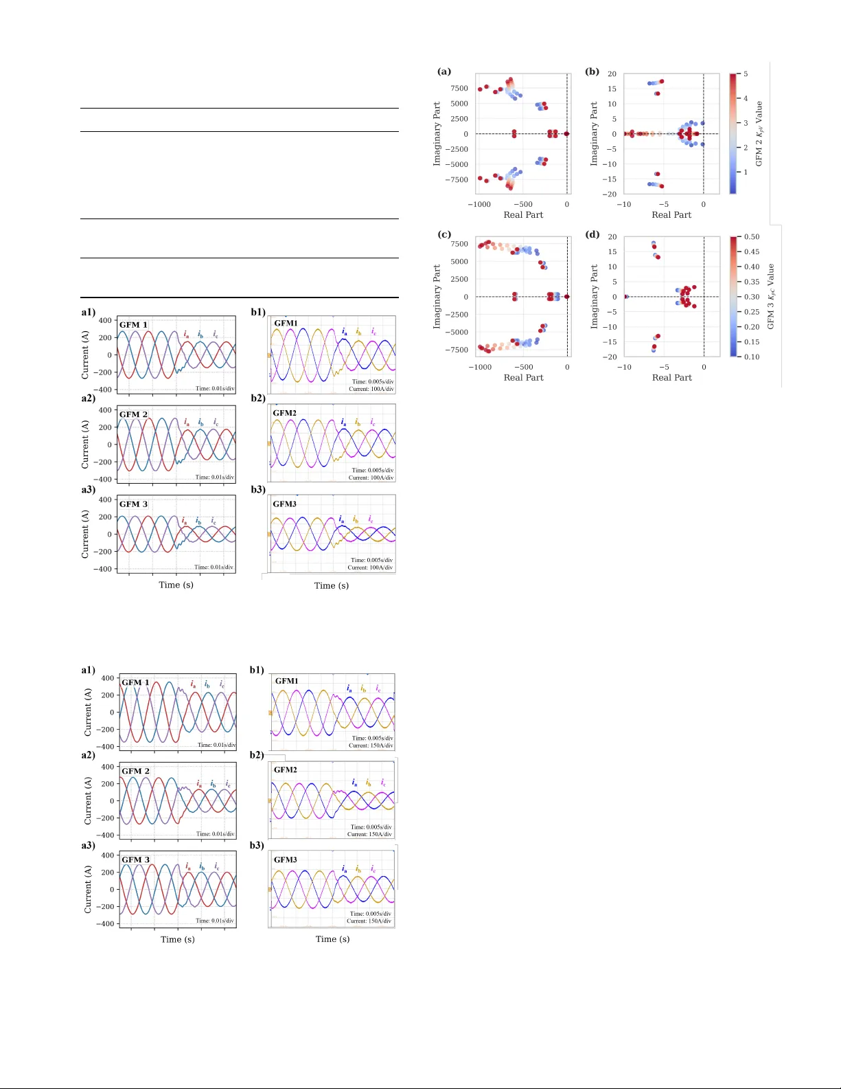
IEEE TRANSA CTIONS ON POWER ELECTR ONICS 1 Disco v ering Unkno wn In v erter Gov erning Equations via Physics-Informed Sparse Machine Learning Jialin Zheng, Member , IEEE, Ruhaan Batta, Student Member , IEEE, Zhong Liu, Student Member , IEEE, Xiaonan Lu, Member , IEEE Abstract —Discovering the unknown governing equations of grid-connected in verters from external measur ements holds sig- nificant attraction for analyzing modern in verter -intensive power systems. Howev er , existing methods struggle to balance the identification of unmodeled nonlinearities with the preservation of physical consistency . T o address this, this paper proposes a Physics-Informed Sparse Machine Learning (PISML) frame- work. The ar chitecture integrates a sparse symbolic backbone to capture dominant model skeletons with a neural residual branch that compensates f or complex nonlinear control logic. Mean- while, a Jacobian-regularized physics-inf ormed training mech- anism is intr oduced to enf orce multi-scale consistency including large/small-scale beha viors. Furthermore, by performing sym- bolic regression on the neural residual branch, PISML achieves a tractable mapping from black-box data to explicit control equations. Experimental results on a high-fidelity Hardware- in-the-Loop platform demonstrate the framework’ s superior performance. It not only achiev es high-resolution identification by reducing error by over 340 times compared to baselines but also realizes the compression of heavy neural networks into compact explicit f orms. This restor es analytical tractability for rigorous stability analysis and reduces computational complexity by orders of magnitude. It also provides a unified pathway to con vert structurally inaccessible devices into explicit mathemat- ical models, enabling stability analysis of power systems with unknown in verter gover ning equations. Index T erms —Grid-forming inv erter , system identification, stability analysis, neural network, physics-inf ormed machine learning, sparse regression. I . I N T R O D U C T I O N T HE rapid proliferation of in verter-based resources (IBRs) is fundamentally reshaping the landscape of modern power systems [1], [2]. As con ventional synchronous machines are increasingly replaced by software-controlled power elec- tronic con verters, grid dynamics are no w dominated by embed- ded control algorithms rather than intrinsic physical properties such as mechanical or electromagnetic coupling [3], [4]. A critical challenge arises because both grid-following (GFL) and grid-forming (GFM) inv erters typically operate with pro- prietary and closed-source control logic, essentially black boxes to grid operators [5], [6]. This structural inaccessibility jeopardizes the effecti veness of traditional stability assessment paradigms, which rely on explicit state-space equations to analyze eigenv alue trajectories and damping characteristics [7]. As a result, a crucial modeling gap is rapidly widening: while in verter penetration continues to increase, theoretical tools for understanding and predicting their dynamic beha viors lag significantly behind [8], [9]. W ith the deployment of advanced sensing technologies such as phasor measurement units (PMUs) and high-bandwidth impedance measurement systems, massive amounts of high- resolution dynamic data have become av ailable, offering new opportunities to uncov er inv erter dynamics from observations [10], [11]. Howe ver , most existing studies still focus on local linear impedance identification [12]. These methods hav e ev olved from traditional frequency sweeping to real- time signal injection (e.g., chirp signals or pseudo-random binary sequences) and can handle complex scenarios such as parallel in verter configurations through sophisticated decoding networks [13], [14]. While these approaches are ef fecti ve in fitting observed data, they inherently assume a locally linear time-in variant (L TI) physical structure and thus fail to capture the global consistency of the underlying nonlinear dynamics [15]. As a result, there are still challenges for critical analytical tasks beyond impedance analysis, such as eigen v alue-based stability assessment or transient stability analysis [16]. For grid operators seeking a comprehensiv e understanding of stability boundaries, relying solely on black-box impedance predictors could be insuf ficient when lar ge-signal dynamics need to be considered. Consequently , there is a strong need for a data-driv en approach capable of discovering explicit control equations gov erning the system dynamics [17]. From a broader scientific perspectiv e, automatically discov- ering the governing equations of nonlinear systems from exter- nal measurements remains a major interdisciplinary challenge [18]. Early approaches such as equation-free modeling and empirical dynamic modeling established foundational ideas but often encountered dif ficulties in scalability and robustness when dealing with high-dimensional and noisy data [19]. With the de velopment of symbolic regression and genetic program- ming, researchers began to directly search the mathematical expression space to reconstruct differential equations [20]. In the field of power and energy systems, symbolic regression has shown potential for identifying battery degradation pro- cesses [21] and extracting reduced-order grid dynamics [22]. Howe ver , symbolic regression implicitly relies on the strong assumption that a predefined function library is sufficiently complete to describe the unkno wn physics. This assumption often fails in high-dimensional multi-time-scale control archi- tectures, where the search space grows exponentially and the sensitivity to noise increases significantly [23]. The emergence of Scientific Machine Learning (SciML) introduced a new paradigm by incorporating physical priors into the learning process. Graph Neural Networks (GNNs) hav e been adopted to capture the topological structure and component interactions within complex power electronic and power system [24]. By explicitly modeling the connectivity , these methods offer scalability to large-scale networks that is difficult to achiev e with standard dense layers [25], [26]. Meanwhile, Neural Ordinary Differential Equations (Neural ODEs) and Univ ersal Differential Equations (UDEs) represent IEEE TRANSA CTIONS ON POWER ELECTRONICS 2 system dynamics through differentiable neural architectures [27], [28]. These methods hav e been used to characterize battery thermal behavior , learn grid frequency responses, and predict dynamic features of power electronic devices [15], [29]–[31].Although these approaches are expressiv e in repre- sentation, purely neural methods often prioritize data fitting, rather than obey physical consistency constraints and guaran- tee physical v alidity [32]. This may result in models that are accurate in prediction but physically inconsistent in structure. Physics-Informed Neural Networks (PINNs) address this issue by integrating physical la ws such as energy conserv ation into the loss function, thereby enhancing generalization under data-scarce conditions [33]–[35]. Howe ver , such constraint enforcement does not necessarily yield interpretable, explicit physical equations, and the learned representations still prove difficult to understand. In summary , the ev olution from impedance identification to symbolic regression and SciML represents a continuous effort to bridge the gap between black-box nonlinear systems and interpretable physical modeling. Ho we ver , each paradigm faces inherent limitations due to assumptions regarding the physical consistency of unkno wn dynamics [36]. Impedance identification assumes local linearity and ignores global non- linear behavior . Symbolic regression assumes a closed-form function structure and struggles with complexity . Neural net- works (NNs) assume data sufficienc y and often sacrifice inter- pretability [37]. Consequently , existing methods frequently fail to maintain consistency across dif ferent dynamic scales, lead- ing to nonphysical beha viors such as inaccurate eigen v alues. Therefore, there is an urgent need for a unified framew ork that ensures nonlinear expressi veness, multi-scale physical consistency , and interpretability . T o ov ercome these limitations, this paper proposes a Physics-Informed Sparse Machine Learning (PISML) frame- work that defines the equation discovery problem for in verter- based systems. The central idea of PISML is a co-design of interpretability and expressiv eness, achieved through a hybrid symbolic–neural structure. The frame work decomposes in verter dynamics into a sparse symbolic backbone, capturing analytically tractable physical laws, and a neural residual NN, modeling complex nonlinearities. Beyond this architectural integration, PISML introduces a physics-informed multi-scale consistency training mechanism that enforces agreement be- tween large-signal trajectory behavior and small-signal per- turbation responses. This deriv ative-le vel constraint grounds the learned model in physically meaningful Jacobian struc- tures, ensuring that both global and local dynamics remain consistent with the underlying physics. Finally , a symbolic regression process extracts explicit closed-form equations from the trained neural model, bridging the gap between black- box data fitting and analytical modeling. Through this unified formulation, PISML enables interpretable, physically consis- tent, and analytically tractable discovery of in verter control equations directly from measurement data. The main contributions of this paper are summarized as follows: 1) Hybrid neural–symbolic ar chitectur e : Integrates a sparse symbolic backbone with neural residual dynamics. This Fig. 1. Problem formulation for identifying grid-connected inverter dynamics. design decouples dominant physical laws from unmod- eled nonlinearities, balancing explicit interpretability with high-fidelity representation. 2) Multi-Scale Dynamic Consistency : Introduces a physics- informed training strategy via perturbation-response con- straints. This ensures the learned model simultaneously achiev es accurate large-signal trajectory reconstruction and physically valid small-signal linearization properties. 3) Interpretable Explicit Discovery : Achieves fidelity- preserving compression of the learned dynamics, transforming over -parameterized neural netw orks into lightweight symbolic equations. This restores analytical tractability for theoretical stability deriv ation. The remainder of this paper is organized as follows. Section II presents the problem formulation for gov erning equation discov ery in po wer electronic systems. Section III introduces the proposed PISML framework. Section IV provides case studies for validation. Finally , Section V concludes the paper . I I . P R O B L E M F O R M U L A T I O N A. Dynamics of Grid-connected Inverter The dynamic beha vior of a grid-connected inv erter is gov- erned by an intricate interaction between its physical power stage and its embedded digital control system. As shown in Fig. 1, the in verter dynamics can be described as a continuous- time nonlinear system, in which the time ev olution of the state vector x ( t ) ∈ R n is defined by a vector field f ( · ) : ˙ x ( t ) = f ( x ( t ) , u ( t )) =  f phy ( x phy , x ctrl , u ) f ctrl ( x phy , x ctrl , u ref )  (1) where x phy represents the physical states (e.g., inductor cur- rents and capacitor voltages), while x ctrl denotes the internal control states (e.g., integrator outputs, phase angles of phase- locked loops or virtual oscillators). The term u ( t ) corresponds to the external excitation such as the grid voltage at the point of common coupling (PCC), and u ref denotes internal control references. The subsystem f phy is deriv ed from Kirchhoff ’ s circuit laws and typically exhibits an analytical and low-order structure. In contrast, the control subsystem f ctrl embodies the algorith- mic logic of control strategies, such as grid-following (GFL) or grid-forming (GFM), introducing significant nonlinearities through coordinate transformations, synchronization mecha- nisms, saturation ef fects, and po wer computation loops, among other specific control functions. B. The Modeling Gap in T raditional Methods In real-world applications, a significant information asym- metry persists between inv erter manufacturers and system op- erators. While the physical stage dynamics f phy are gov erned by established circuit laws, the control structure f ctrl remains IEEE TRANSA CTIONS ON POWER ELECTRONICS 3 Fig. 2. Overview of the Physics-Informed Symbolic Machine Learning (PISML) framework. The approach combines a sparse symbolic backbone with a residual neural ODE to capture unknown dynamics. The model is trained using a composite physics-informed loss function ( L total ), followed by a symbolic regression step to extract an explicit, interpretable ODE representation from the neural residue. strictly proprietary , effecti vely constituting a black box. Con- ventional data-dri ven approaches, particularly impedance iden- tification techniques, typically linearize the system trajectory around a specific operating point x 0 , yielding the approximate form: ∆ ˙ x ≈ A ( x 0 )∆ x + B ( x 0 )∆ u (2) where A ( x 0 ) = ∂ f ∂ x    x 0 denotes the Jacobian matrix at the equi- librium. While such impedance-based linearization methods are adequate for local small-signal analysis, they inherently cannot capture the global nonlinear behavior of the vector field f ( x ) . Consequently , these methods prove insufficient for ev aluating large-signal dynamics, such as transient stabil- ity assessment, fault ride-through capabilities, and scenarios where source-side intermittence driv es the system far from its nominal operating point. The challenge, therefore, extends beyond simple parameter estimation; it demands discovering the explicit functional structure of the gov erning nonlinear dynamics directly from measurement data. C. Mathematical F ormulation of the Equation Discovery The central objective of this study is to discov er the ex- plicit governing equations of an in verter control system from measurement data, as shown in Fig. 1. Giv en a data set D = { t k , x ( t k ) , u ( t k ) } K k =0 , (3) comprising discrete measurements of system trajectories, the goal is to identify a model ˆ f ( x, u ) that satisfies two key requirements. First, it must minimize the trajectory reconstruction error in euclidean norm between the model-predicted and measured states: min ˆ f X k     Z t k t 0 ˆ f ( x ( τ ) , u ( τ )) dτ − x meas ( t k )     2 2 (4) Second, ˆ f must be expressed in symbolic closed form to reflect the underlying physical laws. This renders the problem ill-posed, as multiple candidate functions may exhibit identical data-fitting accuracy while representing distinct local Jacobian structures. Therefore, the discovered model must preserve multi-scale dynamic consistency , reproducing both the global nonlinear response and the local linearization characteristics of the true in verter system. I I I . M E T H O D O L O G Y : T H E P H Y S I C S - I N F O R M E D S PA R S E M AC H I N E L E A R N I N G ( P I S M L ) F R A M E W O R K T o overcome the trade-off between the interpretability of symbolic regression and the representational power of NNs, this work introduces the PISML framew ork. As shown in Fig. 2, PISML integrates a hybrid neural-symbolic architecture with a physics-informed multi-scale learning mechanism to enable interpretable model discov ery . A. Physics-Informed Sparse Symbolic Re gr ession The foundation of the proposed approach lies in the parsi- mony hypothesis of po wer electronic systems [20]. Although the state trajectories of grid-connected in verters exhibit com- plex nonlinear dynamics, their governing equations are not arbitrary mathematical combinations. Instead, they are strictly constrained by electromagnetic principles (e.g., Kirchhoff ’ s laws) and engineered control architectures (e.g., PI regula- tors). This implies that within the high-dimensional space of potential functions, the true vector field f ( x ) is composed of a sparse linear combination of a limited set of specific physical interaction terms. T o explicitly extract this physical structure from data, this paper proposes a matrix-based sparse regression framework, as shown in Fig. 3. First, the state snapshots sampled at time instants t 1 , t 2 , . . . , t K and their time deriv ativ es are arranged into data matrices X ∈ R K × n and ˙ X ∈ R K × n : X =    x ( t 1 ) T . . . x ( t K ) T    , ˙ X =    ˙ x ( t 1 ) T . . . ˙ x ( t K ) T    (5) T raditional symbolic regression approaches often employ generic polynomial libraries to approximate nonlinearities, which ine vitably leads to ov er-parameterization and loss of interpretability [20]. T o address this, the proposed approach discards generic basis functions and proposes a Domain- Specific Physics-Informed Library construction strategy . A candidate function library Θ ( X ) is constructed as the direct sum of physical constitutive terms Θ phy and control functional terms Θ ctrl : Θ ( X ) =  Θ phy ( X ) Θ ctrl ( X )  (6) where the physical sub-library Θ phy comprises the linear state basis describing the fundamental characteristics of the circuits (e.g., RLC filter networks), covering basic state v ariables such IEEE TRANSA CTIONS ON POWER ELECTRONICS 4 Fig. 3. Schematic illustration of the Sparse Identification of Nonlinear Dynamics. The method constructs a library of candidate nonlinear functions Θ ( X ) and employs sparse regression to select the active coefficients Ξ that best describe the time-series data deriv ativ es ˙ X , enabling the reconstruction of the underlying gov erning equations. as currents i dq and voltages v dq . Within the control sub-library Θ ctrl , two critical nonlinear elements are introduced: the bilinear acti ve and reactiv e power calculation terms Θ power , defined as p = v d i d + v q i q and q = v q i d − v d i q , which are essential for capturing GFM or GFL control logic; and the integral state v ariables ξ = R ( x ref − x ) dt , representing the dynamics of integral controllers. Consequently , the augmented feature library is explicitly formulated as: Θ ( x ) = h 1 , x 1 , . . . , x n | {z } Linear/Physical , ξ 1 , . . . , ξ m | {z } Integral Control , v d i d + v q i q | {z } P , v q i d − v d i q | {z } Q i (7) Based on this physics-informed library , the sparse symbolic backbone, f sparse ( x ) , postulates that the time deri vati ve ma- trix ˙ X can be approximated by a sparse linear combination of these library columns: f sparse ( x, u ) = ˙ X ≈ Θ ( X )Ξ (8) where Ξ = [ ξ 1 , ξ 2 , . . . , ξ n ] ∈ R p × n is the coefficient matrix. Each column ξ k determines the activ e terms in the dynamic equation for the k -th state variable. The identification problem is thus cast as a sparse optimization problem: L traj (Ξ) = min Ξ 1 2 ∥ ˙ X − Θ ( X )Ξ ∥ 2 F + λ ∥ Ξ ∥ 1 (9) The ℓ 1 regularization term functions as a physical topology selector . By penalizing the cardinality of non-zero terms, this objectiv e function compels the model to discard redundant terms unnecessary for describing the system dynamics. Con- sequently , the resulting non-zero coefficients do not merely achiev e accurate data reproduction but explicitly rev eal the true physical interconnections and control law structures within the system. B. Neural ODE for Residual Dynamics While the physics-informed sparse backbone effecti vely captures the dominant structural dynamics, constructing a truly exhausti ve library that encompasses all potential proprietary control logic is practically infeasible and would impose pro- hibitiv e data requirements due to the combinatorial explo- sion of candidate terms. Consequently , the symbolic model f sparse ( x, u ) (Eq. 8) serves as a low-order approximation. The discrepancy between the true system dynamics and this sparse backbone is defined as the residual component: ˙ x resid = ˙ x true − f sparse ( x, u ) (10) This residual term ˙ x resid embodies critical high-frequency nonlinear behaviors and unmodeled control logic. T o model this residual dynamics, con ventional data-dri ven approaches typically employ discrete-time sequence models, such as Recurrent Neural Networks (RNNs). Fundamentally , these methods learn a discrete mapping x k 7→ x k +1 . Howe ver , this formulation is intrinsically bound to the training sampling interval ∆ t , lacking the continuous-time definition required for variable step-size integration. Consequently , such models induce discretization errors and fail to interface with standard adaptiv e ODE solvers [15]. T o address this, the proposed framew ork bypasses the dis- crete mapping and directly parameterizes the continuous-time differential equation of the residual using a neural network. As illustrated in Fig. 4, the system states x and external inputs u are fed in parallel into both the sparse symbolic module and the neural network module. Specifically , the residual approximator N ( x, u ; θ N N ) is instantiated as a deep Multilayer Perceptron (MLP). Letting z = [ x T , u T ] T denote the concatenated in- IEEE TRANSA CTIONS ON POWER ELECTRONICS 5 Fig. 4. Architecture of the proposed Neural Residual ODE. This module compensates for the dynamics gap in the sparse backbone by superimposing a learnable neural vector field. The merged derivati ves are integrated via a shared ODE solver , enabling direct end-to-end training using trajectory data. put vector , the layer-wise forward propagation is rigorously defined as:      h (0) = z h ( l ) = σ ( W ( l ) h ( l − 1) + b ( l ) ) , l = 1 , . . . , L − 1 ˙ x resid = W ( L ) h ( L − 1) + b ( L ) (11) where h ( l ) represents the hidden state vector of the l -th layer , and σ ( · ) denotes the element-wise nonlinear activ ation function. The set θ N N = { W ( l ) , b ( l ) } L l =1 constitutes the learnable weights and biases parameters, with the final output layer mapping directly to the unmodeled residual ˙ x resid . The total system dynamics are thus formulated as the superposition of the symbolic vector field and the neural residual vector field: ˙ x ( t ) = f sparse ( x, u ) + N ( x, u ; θ N N ) . (12) This hybrid vector field constitutes a complete ODE system that can be seamlessly embedded into any standard ODE solver . Consequently , the estimated state ˆ x ( t k ) at any time instant t k is obtained by numerically integrating the combined dynamics from the initial condition x ( t 0 ) : ˆ x ( t k ) = x ( t 0 ) + Z t k t 0 (Θ( x ( τ ))Ξ + N ( x ( τ ); u ( τ ); θ N N )) dτ (13) This formulation implies that the model is no longer bound by a fixed discrete step size; instead, it adaptiv ely adjusts the integration step dτ during both training and inference to match the stiffness of the system dynamics, thereby accurately capturing fast transient processes. During training, the objectiv e was to minimize the discrep- ancy between the solver -predicted trajectories and the ground- truth measurements. T o this end, the trajectory reconstruction loss function L traj is defined as: L traj = 1 K K X k =1 ∥ ˆ x ( t k ) − x meas ( t k ) ∥ 2 2 (14) where K denotes the total number of sampling points in the trajectory , x meas ( t k ) represents the measured system state at time t k , and ∥ · ∥ 2 denotes the euclidean norm. T o enable scalable training, the adjoint sensiti vity method [27] is lev eraged. This approach computes gradients by solving an augmented ODE backward in time, thereby decoupling Fig. 5. Multi-time-scale physics-informed training mechanism. memory consumption from integration depth and facilitating efficient end-to-end optimization. C. Multi-T ime-Scale Physics-Informed T raining Mechanism The simultaneous optimization of sparse coefficients Ξ and neural weights θ N N presents a severe identifiability challenge. Due to the universal approximation capability of neural networks, unconstrained joint training often leads to the neural component ov er-parameterizing dominant dynamics that should physically be attrib uted to the symbolic backbone, causing symbolic degradation. T o suppress this competitiv e in- teraction and enforce physical plausibility , a physics-informed joint training strategy is adopted, as sho wn in Fig. 5. W ithin a unified computational graph, Ξ and θ N N are optimized simultaneously , where the separation of duties is driv en by the interplay between structural sparsity constraints and physical property alignment. T o ensure the symbolic backbone prioritizes the capture of dominant physical laws, the joint objective function applies strict ℓ 1 regularization on Ξ while incorporating physical guidance deri ved from the system’ s small-signal characteris- tics. This dual mechanism functions as a precision filter: the sparsity constraint condenses global dynamics into compact analytical expressions, while the small-signal Jacobian consis- tency term forces the linearized features of the hybrid model to align with the true physical system. Under this physical guidance, the neural network is implicitly formulated as a IEEE TRANSA CTIONS ON POWER ELECTRONICS 6 Fig. 6. Schematic of the two-stage identification frame work. The Black Box Stage utilizes a neural predictor as a universal smoother to generate high-fidelity synthetic data from noisy samples. This facilitates the White Box Stage, where sparse symbolic regression is applied to the denoised data to recover an interpretable model consisting of a physical backbone and distilled control logic. residual compensator . It is constrained within the framework of the symbolic backbone, induced to learn only the high- frequency nonlinearities and local disturbances that exceed the representational capacity of the rigid symbolic structure. The total optimization objectiv e integrates macroscopic tra- jectory error , microscopic Jacobian constraints, and a sparsity penalty to jointly regulate both parameter sets: L total = L traj ( θ N N , Ξ) + λ pert L pert ( θ N N , Ξ) + λ sparse ∥ Ξ ∥ 1 (15) Crucially , the term L pert introduces physical guidance by rec- tifying the model’ s eigen v alues through microscopic Jacobian consistency . The total analytical Jacobian of the hybrid model, computed via Automatic Differentiation, explicitly couples the symbolic coefficients Ξ with the neural weights θ N N : J model ( x, Ξ , θ N N ) = Ξ T ∂ Θ( x ) ∂ x + ∂ N ( x, θ N N ) ∂ x (16) This analytical Jacobian is aligned with the empirical small- signal response observed in perturbation data: L pert = ∥ ∆ ˙ x meas − J model ( x meas , Ξ , θ N N )∆ x meas ∥ 2 F (17) Through this coupled optimization, PISML ensures that the learned deriv ati ve field remains consistent with the true sys- tem’ s stability characteristics. This forces Ξ to account for the dominant dynamics that satisfy physical linearization, while θ N N focuses on rectifying unmodeled residual dynamics with- out compromising the physical interpretability of the symbolic backbone. D. Symbolic Explicit Equation Discovery While the hybrid PISML model successfully captures complex system dynamics, the neural residual component N ( x ; θ ∗ N N ) remains an implicit function encoded within thou- sands of weights and bias. T o overcome this barrier , sparse symbolic regression is again applied to the trained NN. This process functions as a symbolic regression mechanism, projecting the high-dimensional neural NN onto a concise set of closed-form mathematical expressions. As illustrated in Fig. 6, this transformation effecti vely con verts the hybrid symbolic/neural model into a computationally efficient and analytically tractable symbolic model, preserving the high fidelity of the neural proxy while recov ering the explicit physical structure required for theoretical analysis. The core rationale is to utilize the trained NN as a high- fidelity predictor . Unlike performing symbolic regression di- rectly on raw , noisy measurements, which severely restricts library complexity due to ov erfitting risks, the NN acts as a univ ersal smoother . It generates a dense, noise-free synthetic dataset (Eq. 3) by interrogating the learned NN: y j = N ( x j ; θ ∗ N N ) (18) This ele v ation in data quality permits the deployment of an extended function library Θ ext ( x ) . In contrast to the compact library used for the backbone, Θ ext ( x ) is enriched with a comprehensiv e spectrum of nonlinear candidates, including high-order polynomials, trigonometric functions ( sin , cos ), and rational terms, which are indispensable for characterizing proprietary control logic such as Phase-Locked Loops (PLLs). Lev eraging this pristine synthetic data, a secondary sparse regression problem is formulated to identify the explicit struc- ture Ξ ∗ resid of the residual using Eq. 9. Finally , the distilled symbolic residual is merged with the original sparse backbone to yield the discov ered gov erning equation: ˆ f f inal ( x ) = Θ( x )Ξ ∗ + Θ ext ( x )Ξ ∗ resid (19) This formulation represents a complete, closed-form recon- struction of the underlying system. Crucially , since the neural predictor was trained under Jacobian consistency constraints ( L pert ), the deriv ed explicit equation ˆ f f inal ( x ) inherits the correct local stability characteristics, thereby bridging the gap between data-driv en modeling and rigorous theoretical analysis. I V . C A S E S T U D I E S : G R I D - C O N N E C T E D I N V E RT E R W I T H U N K N OW N G OV E R N I N G E Q UAT I O N S A. Case Study Setup T o comprehensively ev aluate the identification capability of the proposed framew ork under realistic conditions, a high- fidelity Hardware-in-the-Loop (HIL) testing en vironment is established. The target system comprises a GFM inv erter connected to a stiff grid via an LCL filter , a topology widely adopted in modern power electronic-dominated grids. The standard GFM dynamic model, as documented in [38] is adopted; this model features a droop control mechanism with cascaded voltage and current loops. The detailed circuit and control parameters utilized in this study are illustrated in Fig. 7 (a) and listed in T able I, serving as the ground truth for IEEE TRANSA CTIONS ON POWER ELECTRONICS 7 T ABLE I P A R AM E T E RS O F T H E G R ID - F O RM I N G I N V ERT E R T ES T S Y S TE M Parameter Symbol V alue Unit System Ratings Base Po wer S base 500 kV A Base V oltage (Line-Line) V base 480 V Nominal Frequency f nom 60 Hz LCL F ilter & Grid Impedance In verter -side Inductance L f ( L i ) 0.10 p.u. In verter -side Resistance R f ( R i ) 0.02 p.u. Filter Capacitance C f 0.05 p.u. Damping Resistance R d 0.05 p.u. Grid-side Inductance L g ( L p ) 0.05 p.u. Grid-side Resistance R g ( R p ) 0.01 p.u. Contr ol P arameters Activ e Po wer Droop Gain m p 0.05 p.u. Reactiv e Po wer Droop Gain m q 0.05 p.u. Power Filter Cut-off Freq. ω c 10 π rad/s V oltage Loop PI Gains K pV , K iV 0.8, 3.0 - Current Loop PI Gains K pC , K iC 0.2, 4.0 - validation, although the specific control structure is treated as a black box during the identification process. The data acquisition and training pipeline relies on a hybrid digital-analog platform, as depicted in Fig. 7 (b). The po wer stage dynamics are emulated on a T yphoon HIL404/604 series real-time simulator, while physical control signals are cap- tured via high-bandwidth oscilloscopes to incorporate realistic measurement noise before being processed on a workstation equipped with an NVIDIA A100 GPU for accelerated PISML training. Data is sampled at 10 kHz. T o generate a training data set rich in transient dynamics and pre vent the model from ov erfitting to trivial equilibrium points, random perturbations at the PCC are introduced. These excitations include voltage sags ranging from 0.8 to 1.0 p.u. and phase angle jumps between 5 and 10 degrees, ensuring the learned model remains valid across a wide operating range. The performance of the proposed PISML is benchmarked against three distinct identification paradigms, with imple- mentation details summarized in T able II. The comparativ e group includes Standard SINDy using a generic polynomial library , representing con ventional sparse identification without domain adaptation; Pure Neural ODE, representing a fully Fig. 7. Experimental implementation of the proposed framework. (a) Schematic of the single-GFM inv erter training pipeline for ODE extraction. (b) The physical hardware experimental platform employed for single-GFM in verter and multi-GFM inv erters validation. black-box approach lacking physical constraints; and Mod- SINDy . Notably , Mod-SINDy utilizes the physics-informed domain library constructed in this work but relies exclusiv ely on sparse symbolic regression. It effecti vely serves as the symbolic backbone of the proposed framework, isolating the contribution of the neural residual correction in the ablation analysis. B. T rajectory Reconstruction & Generalization The trajectory reconstruction capability of the proposed PISML frame work is ev aluated under data-scarce conditions. T o emulate practical limitations in acquiring grid-connected data, the training dataset is strictly limited to 12 trajectories sampled within a conservati ve operating range of voltage magnitude u ∈ [0 . 8 , 1 . 2] p.u. The trained models are then assessed on a se vere dynamic test scenario where the system undergoes a large-signal step disturbance dropping to 0 . 4 p.u. This drastic voltage sag pushes the system state far into the Out-of-Distribution (OOD) region, representing a significantly more rigorous test of generalization than static operating point variations. T ABLE II C O MPA R IS O N O F I D E NT I FI CAT IO N M E TH O D S A N D H Y P E RPA R AM E T E R S E TT I N G S Method Architectur e / Library Optimizer & Regularization Key Settings Baseline A: Library: Polynomial (Degree 2) Solv er: STLSQ Threshold: 0.005 Standard SINDy Features: 120 (approx.) Reg: Sparse Thresholding Preproc: MinMaxScaler Baseline B: Library: Physics-Informed Solver: Ridge Regression α : 1 × 10 − 6 Mod-SINDy Features: Linear + Bilinear Po wer Reg: L2 Norm Preproc: MinMaxScaler Baseline C: Net: MLP (3 Layers) Optimizer: AdamW LR: OneCycle (Max 0.005) Pure NODE Dim: 14 → 128 → 128 → 13 Loss: MSE Epochs: 50 Activ ation: T anh Norm: LayerNorm Preproc: StandardScaler Proposed: 1) Sparse Backbone: Solver: Ridge ( α = 0 . 1 ) Library: Physics-Based PISML 2) Neural Residual: Optimizer: AdamW LR: OneCycle (Max 0.005) Net: MLP (3 Layers) W eight Decay: 1 × 10 − 3 Dropout: 0.05 Dim: 14 → 128 → 128 → 13 Norm: LayerNorm Epochs: 50 IEEE TRANSA CTIONS ON POWER ELECTRONICS 8 Fig. 8. Comparison of trajectory reconstruction for a GFM inv erter. (a) v d . (b) v q . (c) i d . (d) i q . The green region ( t < 0 . 02 s) indicates in-distribution training data, while the red region ( t ≥ 0 . 02 s) ev aluates out-of-distribution (OOD) generalization under a lar ge-signal step disturbance. Fig. 9. Trajectory reconstruction for a GFM inverter with nonlinear dual-loop limiting. (a) v d . (b) v q . (c) i d . (d) i q . The green region evaluates in-distribution performance, while the red region tests OOD generalization under control saturation. T ABLE III E R RO R C O M P A R I S ON U N D ER S TAN D AR D A N D S A T U R A T I O N S C E NA R IO S Method Standard Unknown Sat. IOD (%) OOD (%) IOD (%) OOD (%) Std SINDy 29.65 150.36 207.63 934.63 Mod-SINDy 7.10 90.83 68.47 483.03 Pure NODE 6.48 104.82 6.26 120.29 PISML 0.59 1.94 0.92 2.95 Note: IOD: In-Distribution (0–0.02s); OOD: Out-of-Distrib ution (0.02–0.04s). “Unknown Sat. ” refers to unmodeled control saturation. The metric is the Relativ e L 2 Norm a veraged over [ i d , i q , v d , v q ] , calculated as ϵ = ( ∥ ˆ y − y ∥ 2 / ∥ y ∥ 2 ) × 100% , where ˆ y is the estimate and y is the ground truth. The time-domain reconstruction results for the standard GFM model are presented in Fig. 8. Standard SINDy exhibits significant steady-state deviation and transient errors due to the inherent stiffness and multi-time-scale nature of GFM dynamics; the generic polynomial library lacks the capacity to sparsely represent the complex trigonometric couplings and bilinear power terms essential to the control topology . In the OOD region ( t ≥ 0 . 02 s), the limitations of pure data-driv en methods become pronounced. Although the Pure Neural ODE maintains a reasonable approximation within the training distribution, its tracking error increases visibly in the OOD region, confirming its inability to extrapolate dynamics correctly without physical inductiv e bias. Mod-SINDy , while incorporating physical terms, suffers from library truncation error during deep voltage sags. In contrast, PISML achie ves high-fidelity tracking in both regions by le veraging the sparse physical backbone for robust extrapolation and the neural residual for precision. T o further probe the limits of identifiability , the methods are ev aluated on a GFM system containing unknown non-linear saturation blocks in the control loops, with the corresponding trajectory comparisons illustrated in Fig. 9. As summarized in T able III, both symbolic baselines suffer catastrophic per- formance degradation, yielding OOD errors exceeding 400% . This failure stems from the fundamental inability of basis functions library to represent hard nonlinearities, resulting in erroneous global polynomial fitting. In contrast, the Pure Neural ODE exhibits inherent adaptability to such non-smooth functions due to its univ ersal approximation capability , av oid- ing the diver gence observed in symbolic methods. Howe ver , PISML achieves the superior performance with an OOD error of only 2 . 95% . This confirms that the neural residual compo- nent effecti vely compensates for the hard non-linearities and discontinuous behaviors that the symbolic backbone cannot resolve, while the backbone ensures stability in the linear regions. C. Data Efficiency and Noise Robustness Subsequently , the data efficiency of the competing paradigms is quantified. Fig. 10 depicts the e volution of reconstruction errors with respect to the training dataset size. Remarkably , Standard SINDy exhibits a counter -intuiti ve trend where identification performance degrades as data volume increases. This pathology arises because, lacking a complete basis representation for the complex GFM dynamics, the regression algorithm minimizes residuals by overfitting mea- surement noise through high-order polynomials rather than capturing the underlying physics. While Mod-SINDy main- tains stability due to domain-specific priors, it reaches an early performance saturation. Pure NODE adheres to a typical data scaling law , requiring approximately 64 trajectories to match the accuracy that PISML achieves with merely 12. PISML demonstrates superior data efficienc y , con verging to the noise floor with minimal samples. This efficienc y is intrin- sic to its decoupled architecture, where the physical backbone rapidly locks onto dominant dynamics, allowing the neural IEEE TRANSA CTIONS ON POWER ELECTRONICS 9 Fig. 10. Comparison of data efficiency across different modeling frameworks. (a) IOD relative error versus number of trajectories. (b) OOD relativ e error versus number of trajectories. Fig. 11. Robustness analysis under varying noise conditions. (a) IOD relative error versus noise condition (SNR in dB). (b) OOD relative error versus noise condition. T ABLE IV Q UA N TI TA T I V E E V A L UA T I ON O F D I ST R I BU T I ON A L S H I FT V I A W A S S ER S T E IN D I S T A N C E Method W asserstein Dist. Relative Ratio (Lower is Better) (vs. PISML-Phy) Baseline A (Std SINDy) 120.5296 544 . 1 × Baseline B (Mod-SINDy) 83.8019 378 . 3 × Baseline C (Pure NODE) 168.4744 760 . 6 × PISML (w/o Constraints) 75.6735 341 . 6 × PISML-Phy (Proposed) 0.2215 1.0 × Note: The W asserstein Distance (WD) quantifies the discrepancy between the predicted trajectory distribution and the ground truth. The relative ratio indicates how many times larger the distributional error is compared to the proposed PISML-Phy method. A ratio of 1 . 0 × represents the benchmark performance. component to dedicate its capacity solely to resolving residual mismatches. The robustness against measurement noise is ev aluated by training models on raw data corrupted with varying Signal- to-Noise Ratios (SNR) without pre-filtering, as shown in Fig. 11. Symbolic methods re veal a critical vulnerability to noise-induced instability . Standard SINDy div erges rapidly ev en under moderate noise levels due to deri vati ve noise amplification, where numerical differentiation creates spuri- ous high-magnitude targets for the regression. Although Pure NODE av oids di ver gence, it tends to ov erfit high-frequency noise components, resulting in non-physical oscillations. In contrast, PISML demonstrates e xceptional noise tolerance. The enforcement of Jacobian regularization combined with the ℓ 1 sparsity penalty on physical coefficients acts as a physics- informed filter, effecti vely suppressing the identification of spurious noise terms while preserving the fidelity of the true system dynamics. D. Small-Signal Physical Consistency Beyond accurate trajectory reconstruction, preserving small- signal stability is a critical requirement for power electronic modeling. Pure time-domain re gression often fails to guarantee the v alidity of the underlying Jacobian matrix. Therefore, this subsection rigorously e valuates the small-signal behavior of the identified models. For a fair comparison, the baselines utilize their optimal data configurations, with Standard SINDy and Mod-SINDy using 9 trajectories and Pure NODE us- ing 64 trajectories to maximize data-driv en potential. The proposed PISML employs only 12 trajectories to highlight data efficienc y . The standard PISML and the Physics-informed PISML, denoted as PISML-Phy , are compared to isolate the contribution of the Jacobian regularization mechanism, as detailed in Section III-C. First, a Jacobian linearization of the trained models is performed at an operating point of u = 0 . 8 p.u., with the resulting eigenv alue distributions illustrated in Fig. 12. Although Pure NODE, Mod-SINDy , and the unconstrained PISML achiev e acceptable time-domain fitting, their eigenv al- ues exhibit irregular scattering with multiple poles erroneously located in the right-half plane. This spectral pollution implies mathematical instability despite apparent short-term accuracy . A v alid control equation must correctly encode the local vector field structure. In contrast, PISML-Phy successfully eliminates these spurious modes. Its eigen values cluster tightly around the analytical ground truth and remain strictly within the left- half plane. This confirms that the regularization term L pert effecti vely constrains the deri vati ve space and forces the neural residual to respect physical stability boundaries. T o quantify the discrepancy between the true and identified spectra, the W asserstein Distance is employed as listed in T able IV. The unconstrained PISML exhibits a W asserstein metric comparable to the baselines despite superior trajectory reconstruction, indicating limited improv ement in small-signal fidelity . Howe ver , the introduction of the physical guidance mechanism in PISML-Phy yields a transformativ e improve- ment, reducing the distance by a factor of over 340. This em- pirical result proves that physical constraints are indispensable for identifying correct deri vati ves from sparse data. Finally , the robustness of these characteristics is ev aluated across varying operating points in Fig. 13. While the spectral error for all methods naturally increases as the system shifts from the IOD to the OOD region, PISML-Phy consistently maintains the lowest distance by orders of magnitude. This demonstrates that the proposed physical constraints ensure the identified NN remains topologically consistent with the true physics across the entire operating en velope. E. Interpretable Explicit Equation Discovery The ultimate objective of the PISML framew ork is to transcend the intermediate grey-box representation and achie ve fidelity-preserving compression. While the PISML model at- tains high accuracy via the neural residual, it relies on thou- sands of opaque parameters. T o restore analytical transparency , the symbolic distillation is performed on the neural residual component and merge it with the symbolic backbone to extract a compact, explicit mathematical structure. The ev olution IEEE TRANSA CTIONS ON POWER ELECTRONICS 10 Fig. 12. Comparativ e analysis of small-signal stability and eigenv alue distributions across (a) Std SINDy , (b) Mod SINDy , (c) Pure NODE, (d) PISML, and (e) PISML-Phy . Ro ws (a1)–(e1) show the large-signal trajectory of v d . Rows (a2)–(e2) and (a3)–(e3) illustrate global and magnified eigenv alue distributions, respectiv ely , where grey ’x’ markers denote the analytical ground truth. Fig. 13. Robustness analysis of eigenv alue prediction under varying operating points u ∈ [0 . 2 , 1 . 2] . The grouped bar chart illustrates the W asserstein dis- tance (WD) relativ e to the ground truth for fi ve different modeling frame works. of this discovery process is visualized in Fig. 14 (a)–(d). As evidenced by the coefficient heatmaps, the PISML-Phy (Fig. 14b) successfully captures the dominant linear state dependencies, establishing a rigid physical skeleton. Subse- quently , the regression output deriv ed from the neural residual (Fig. 14c) does not produce a dense matrix of spurious terms but selectively identifies the specific nonlinear coupling terms initially unmodeled by the physical backbone. The PISML model (Fig. 14d) seamlessly integrates these components, reconstructing a sparse topology that is structurally isomorphic to the Ground T ruth (Fig. 14a). This structural alignment prov es that PISML has ef fectiv ely learned the underlying physical causality rather than merely ov erfitting the dataset. T o validate that this transition from a neural proxy to an explicit equation incurs no loss of dynamic fidelity , a rigorous performance sweep was conducted across a grid voltage range of 0.2 p.u. to 1.0 p.u. As illustrated in the time- domain trajectories of Fig. 14 (e)–(h), the distilled explicit model (dashed lines) exhibits near-perfect ov erlap with the Ground T ruth (solid lines) ev en under se vere voltage dip and recov ery scenarios. The quantitati ve error analysis is detailed in T able V. The results rev eal that the regression process incurs negligible information loss, as the av erage relativ e errors for activ e power ( P f ) and voltage ( v cd ) are merely 0.58% and 0.88%, respectively .Beyond trajectory matching, true interpretability requires the preservation of local stability characteristics. The eigen value distributions in Fig. 14 (i)–(l) demonstrate that the modes of the distilled model (marked with ‘x’) align precisely with the Ground T ruth (marked with ‘o’). This strict alignment across both lo w-frequency dominant modes and high-frequency oscillatory modes confirms that the discov ered equation accurately reproduces the system’ s mi- croscopic differential geometry , allowing the deriv ed explicit form to serve as a reliable instrument for theoretical stability assessment. T o rigorously quantify the trade-of f between model parsi- mony and predictiv e capability , a statistical ev aluation was performed across different modeling frameworks. As system- atically ev aluated in T able VI, con verting the neural repre- sentation into symbolic terms deli vers transformati ve benefits. Regarding model complexity , PISML achiev es a compression ratio exceeding 250 times by reducing the parameter count from thousands to fewer than fifty coefficients. This extreme sparsity makes the model lightweight enough for embedded DSP controllers. In the trade-off space illustrated in Fig. 15, Standard SINDy falls into the high-error region, while Pure Neural ODE resides in the high-complexity region with poten- tial overfitting risks. Distinct from these approaches, PISML identifies the minimal set of acti ve physical terms, achie ving a fa vorable balance of low complexity and low error . This ensures superior robustness in out-of-distribution scenarios where high-complexity models tend to diver ge. IEEE TRANSA CTIONS ON POWER ELECTRONICS 11 Fig. 14. Evaluation of discovered interpretable d equations. (a)–(d) Sparse coefficient matrices for Ground T rue, PISML-Phy , PISML-Distilled, and Final PISML models. The horizontal axis is categorized into two libraries: the Linear Library comprises the constant bias and 13 state variables ( x 0 , . . . , x 12 ), while the Nonlinear Library consists of 13 candidate functions including bilinear coupling terms (e.g., x k ∆ P ), trigonometric grid voltage terms ( u g cos δ, u g sin δ ), and instantaneous po wer calculation terms. (e)–(h) Comparison of time-domain trajectories for P f and v cd (Solid: Ground T rue; Dashed: PISML-Distilled). (i)–(l) Global and zoomed eigenv alue distributions, where ’o’ and ’x’ markers denote Ground T rue and PISML-Distilled modes, respectiv ely . Fig. 15. Pareto analysis of model robustness versus complexity , comparing PISML variants against black-box NNs and standard sparse regression base- lines. T ABLE V R E LAT IV E E R RO R A NA LYS I S O F H Y B RI D A N D D I ST I L L ED M O D EL S U N DE R V O LT A G E V A R I A T I ON S Grid V oltage u (p.u.) Hybrid Model Error (%) Distilled Model Error (%) Activ e Po wer V oltage v d Activ e Po wer V oltage v d 0.2 0.6371 0.4884 0.1457 1.0081 0.4 0.3653 0.2174 0.2086 1.5530 0.6 0.1430 0.8854 0.4157 1.3209 0.8 0.3493 1.0561 0.4206 0.0521 1.0 0.8709 0.1849 0.4034 0.7935 1.2 0.1823 0.3840 1.8943 0.6020 A verage 0.4246 0.5360 0.5814 0.8883 T ABLE VI C O MP R E H EN S I VE E FFI C I EN C Y & F I D EL I T Y C O M P A R IS O N Metric Pure NODE PISML-Phy PISML-Distilled Model T ype Black-box Grey-box White-box Small-Signal Error High (Unstable) Lo w Low Parameter Count ∼ 5,000+ ∼ 5,000+ < 50 (Coeffs) Analyticity Intractable Intractable T ractable Fig. 16. Schematic diagrams of 3-Buses microgrid topology for validating the interaction between the learned target model and known auxiliary units. F . System-Level Integr ation & Applications The definitiv e advantage of extracting explicit governing equations lies in the capability to integrate the identified model into broader power system simulations. By translating propri- etary black-box devices into a unified mathematical language, PISML empowers grid operators to integrate equipment from div erse manufacturers onto a single platform for full-system analysis. This inte gration capability ensures that the discov ered model is not only accurate for time-domain simulation but also reliable for rigorous theoretical stability assessment. T o v alidate this capability experimentally , a heterogeneous 3-bus microgrid system is constructed, as illustrated in Fig. 16. The topology consists of the identified T arget GFM (repre- sented by the PISML-distilled explicit equations) integrated with two Auxiliary GFMs (Aux GFM 1 & 2) possessing known structures and parameters. The detailed system param- eters are listed in T able VII. This setup, implemented on the HIL platform sho wn in Fig. 7, serves as a rigorous testbed to ev aluate the interaction between the ”learned” dynamics and the ”known” physics. First, the accuracy of the PISML model in a multi-conv erter en vironment is validated through large-signal disturbance test- IEEE TRANSA CTIONS ON POWER ELECTRONICS 12 T ABLE VII S Y ST E M A N D C O NT RO L P AR A M ET E R S C O N FI GU R A T I O N Category Parameter Symbol GFM 1 GFM 2 GFM 3 Control Activ e Droop m p 0.03 0.06 0.05 V oltage Prop. Gain K pV 1.60 2.00 1.40 V oltage Int. Gain K iV 3.00 4.00 2.00 Current Prop. Gain K pC 0.50 0.30 0.40 Current Int. Gain K iC 4.00 4.00 4.00 Line Line Resistance R line 0.01 0.01 0.01 Line Inductance L line 0.001 0.001 0.001 Load Load Resistance R load 0 . 9 Load Inductance L load 0 . 4358 Fig. 17. Experimental validation of system-level transient dynamics in the 3- bus microgrid under a sudden load step. (a1)-(a3) Ground truth output current wav eforms measured from the HIL testbench for the T arget GFM 1, Aux GFM 2, and Aux GFM 3, respectiv ely . (b1)-(b3) Corresponding current trajectories predicted by the PISML-based hybrid simulation. Fig. 18. Experimental validation of system-level transient dynamics in the 3- bus microgrid under a sudden load step. (a1)-(a3) Ground truth output current wav eforms measured from the HIL testbench for the T arget GFM 1, Aux GFM 2, and Aux GFM 3, respectiv ely . (b1)-(b3) Corresponding current trajectories predicted by the PISML-based hybrid simulation. Fig. 19. System-level eigenv alue trajectories (root loci) of the heterogeneous 3-bus microgrid system under control parameter v ariations. (a)-(b) Impact of varying the voltage proportional gain ( K pV ) of Aux GFM 2 on global and dominant modes. (c)-(d) Impact of varying the current proportional gain ( K pC ) of Aux GFM 3. ing. A sudden load step change is applied at t = 0 . 02 s. T o rigorously assess the model’ s robustness against varying external dynamics, the system response is simulated under different control parameter settings for the auxiliary analytical GFM in verters, as illustrated in Fig. 17 and Fig. 18. In both scenarios, the output current waveforms demonstrate that the hybrid model (PISML T arget + Analytical Auxiliaries) closely tracks the HIL ground truth. This consistency confirms that the PISML-derived equation, despite being trained solely on single-unit data, successfully captures the device’ s intrinsic port behaviors and correctly reproduces the transient load- sharing dynamics when interacting with the wider grid. Beyond these time-domain results, the explicit nature of the PISML model enables safe and rapid stability assessment for operations that would be hazardous to perform directly on physical hardware. Specifically , before physically connecting a black-box in verter , operators can mathematically analyze how its integration affects global system stability . T o demonstrate this, a global eigenv alue analysis of the assembled 3-bus system is conducted. The migration of system eigenv alues is in vestigated by tuning the control coefficients of the known units—specifically , the voltage proportional gain ( K pV ) and integral gain ( K iV ) of the auxiliary GFMs. As visualized in Fig. 19, the resulting root locus plot re veals the precise trajectory of the system’ s dominant modes. This analysis allows operators to identify stability boundaries and optimize the settings of existing assets to accommodate the black-box target. Such theoretical insight, deriv ed directly from the math- ematical integration capability of the PISML model, bridges the methodological gap between data-driven identification and rigorous power system engineering. V . C O N C L U S I O N This paper proposes the PISML frame work to bridge the critical modeling gap in power electronics-dominated grids. IEEE TRANSA CTIONS ON POWER ELECTRONICS 13 By synergizing a sparse symbolic backbone with a neural residual branch under Jacobian-regularized physics-informed training, PISML successfully reconciles the inherent con- flict between identifying unmodeled hard non-linearities and preserving physical consistency . Furthermore, the framew ork advances the fidelity-preserving regression of implicit neural dynamics into compact gov erning equations restores analytical tractability for algebraic stability design, while drastically reducing complexity for efficient deployment. The framework was rigorously v alidated on a high-fidelity HIL platform across multiple dimensions, including large-signal trajectory reconstruction, small-signal spectral analysis, and system-lev el integration capability . Quantitativ e results confirm that the proposed method reduces identification error by ov er 340 times compared to symbolic baselines and improves spectral fidelity by two orders of magnitude. By distilling implicit black-box dynamics into explicit control equations, PISML achiev es a breakthrough in integration capability , empowering grid oper- ators to integrate proprietary devices into rigorous eigenv alue analysis workflo ws. Future work will extend this approach to identify complex grid-forming topologies under unstructured grid faults and explore online adaptiv e implementations. R E F E R E N C E S [1] S. Xu et al. , “Revie w of po wer system support functions for inverter - based distributed energy resources- standards, control algorithms, and trends, ” IEEE Open Journal of P ower Electr onics , vol. 2, pp. 88–105, 2021. [2] Y . Lin et al. , “Pathways to the next-generation power system with in verter -based resources: Challenges and recommendations, ” IEEE Elec- trification Magazine , vol. 10, no. 1, pp. 10–21, 2022. [3] Y . Huang et al. , “Physics insight of the inertia of power systems and methods to provide inertial response, ” CSEE Journal of P ower and Ener gy Systems , v ol. 8, no. 2, pp. 559–568, 2022. [4] Y . Qi et al. , “Synthetic inertia control of grid-connected inverter con- sidering the synchronization dynamics, ” IEEE T ransactions on P ower Electr onics , vol. 37, no. 2, pp. 1411–1421, 2022. [5] M. Nestor et al. , “Data-driven communication and control design for distributed frequency regulation with black-box in verters, ” 2025. [Online]. A vailable: https://arxiv .org/abs/2510.17769 [6] R. Rosso et al. , “Grid-forming con verters: Control approaches, grid- synchronization, and future trends—a revie w , ” IEEE Open Journal of Industry Applications , v ol. 2, pp. 93–109, 2021. [7] U. Markovic et al. , “Partial grid forming concept for 100% in verter - based transmission systems, ” in 2018 IEEE P ower & Ener gy Society General Meeting (PESGM) , pp. 1–5, 2018. [8] N. Hatziargyriou et al. , “Definition and classification of po wer system stability – revisited & e xtended, ” IEEE T ransactions on P ower Systems , vol. 36, no. 4, pp. 3271–3281, 2021. [9] T . C. Green et al. , “Zero-inertia power systems: Data-driven stability assessment, ” IEEE P ower and Energy Magazine , vol. 18, no. 2, pp. 56– 65, 2020. [10] L. He et al. , “ A neural network-based online parameter identification method for fractional-order power electronics, ” IEEE T ransactions on Cir cuits and Systems I: Re gular P apers , vol. 72, no. 9, pp. 4868–4876, 2025. [11] I. Kamwa et al. , “Pmu configuration for system dynamic performance measurement in large, multiarea power systems, ” IEEE T ransactions on P ower Systems , vol. 17, no. 2, pp. 385–394, 2002. [12] X. W ang et al. , “Unified impedance model of grid-connected voltage- source con verters, ” IEEE T ransactions on P ower Electronics , vol. 33, no. 2, pp. 1775–1787, 2018. [13] X. W eng et al. , “Chirp signal injection method and real-time impedance characteristic measurement of electric energy router, ” IEEE Journal of Emer ging and Selected T opics in P ower Electronics , vol. 10, no. 5, pp. 5564–5577, 2022. [14] H. Gong et al. , “Dq-frame impedance measurement of three-phase con verters using time-domain mimo parametric identification, ” IEEE T ransactions on P ower Electr onics , vol. 36, no. 2, pp. 2131–2142, 2021. [15] J. Zheng et al. , “Latent-feature-informed neural ode modeling for lightweight stability ev aluation of black-box grid-tied inv erters, ” IEEE T ransactions on P ower Electr onics , pp. 1–6, 2025. [16] Y . Gu et al. , “Power system stability with a high penetration of inverter - based resources, ” Proc. IEEE , vol. 111, no. 7, pp. 832–853, 2023. [17] J. Zheng et al. , “Neural surrogate solver for ef ficient edge inference of power electronic hybrid dynamics, ” IEEE T ransactions on Industrial Electr onics , pp. 1–6, 2026. [18] H. W ang et al. , “Scientific discovery in the age of artificial intelligence, ” Natur e , vol. 620, no. 7972, pp. 47–60, 2023. [19] K. Course et al. , “State estimation of a physical system with unknown governing equations, ” Nature , vol. 622, no. 7982, pp. 261–267, 2023. [20] S. L. Brunton et al. , “Discovering governing equations from data by sparse identification of nonlinear dynamical systems, ” Proceedings of the National Academy of Sciences , vol. 113, no. 15, pp. 3932–3937, 2016. [21] N. Hadifar et al. , “Data-driv en modeling of po wer electronic converters using symbolic regression for digital twin applications, ” in 2025 IEEE Electric Ship T echnologies Symposium (ESTS) , pp. 135–142, 2025. [22] A. T . Sari ´ c et al. , “Symbolic re gression for data-driven dynamic model refinement in po wer systems, ” IEEE T ransactions on P ower Systems , vol. 36, no. 3, pp. 2390–2402, 2021. [23] X. Shi et al. , “Physical-informed detailed aggregation of wind farm based on symbolic regression: Structure, solution and generalizability , ” IEEE T ransactions on Sustainable Energy , pp. 1–14, 2025. [24] K. Egan et al. , “ Automatically discovering ordinary differential equa- tions from data with sparse regression, ” Communications Physics , vol. 7, no. 1, p. 20, 2024. [25] Q. Guo et al. , “Physics-informed neural network combined with sparse identification nonlinear dynamics for battery soc estimation, ” in 2025 IEEE International Confer ence on En vir onment and Electrical Engineer- ing and 2025 IEEE Industrial and Commercial P ower Systems Eur ope (EEEIC / I&CPS Europe) , pp. 1–6, 2025. [26] G. W . Koo et al. , “Efficient algorithm based on sindy-pinn-pso for trans- former air-gap design in obc, ” IEEE T ransactions on P ower Electronics , vol. 41, no. 1, pp. 56–60, 2026. [27] R. T . Chen et al. , “Neural ordinary differential equations, ” Advances in neural information processing systems , vol. 31, 2018. [28] C. Rackauckas et al. , “Universal differential equations for scientific machine learning, ” arXiv preprint , 2020. [29] Z. Liu et al. , “Dissipation-based dynamics-aware learning scheme for transient stability analysis of networked black-box grid-forming in vert- ers, ” IEEE Tr ansactions on P ower Electr onics , vol. 41, no. 3, pp. 3165– 3170, 2026. [30] J. Zheng et al. , “Stability evaluation of black-box grid-forming inv erters via physical-informed neural ordinary dif ferential equations, ” in 2025 IEEE Energy Conversion Conference Congress and Exposition (ECCE) , pp. 1–5, 2025. [31] J. Zheng et al. , “Physics-embedded neural odes for sim-to-real edge digital twins of hybrid power electronics systems, ” IEEE T ransactions on Industrial Electr onics , pp. 1–12, 2026. [32] Y . Lian et al. , “Physically consistent multiple-step data-driv en predic- tions using physics-based filters, ” IEEE Contr ol Systems Letters , vol. 7, pp. 1885–1890, 2023. [33] B. Huang et al. , “ Applications of physics-informed neural networks in power systems - a re view , ” IEEE T ransactions on P ower Systems , v ol. 38, no. 1, pp. 572–588, 2023. [34] G. E. Karniadakis et al. , “Physics-informed machine learning, ” Natur e Reviews Physics , vol. 3, no. 6, pp. 422–440, 2021. [35] Y . Fassi et al. , “T oward physics-informed machine-learning-based pre- dictiv e maintenance for po wer con verters—a revie w , ” IEEE T ransactions on P ower Electr onics , vol. 39, no. 2, pp. 2692–2720, 2024. [36] S. Kole v et al. , “Physically consistent state estimation and system identi- fication for contacts, ” in 2015 IEEE-RAS 15th International Conference on Humanoid Robots (Humanoids) , pp. 1036–1043, 2015. [37] F .-L. Fan et al. , “On interpretability of artificial neural networks: A survey , ” IEEE T ransactions on Radiation and Plasma Medical Sciences , vol. 5, no. 6, pp. 741–760, 2021. [38] N. Pogaku et al. , “Modeling, analysis and testing of autonomous operation of an inv erter-based microgrid, ” IEEE T ransactions on power electr onics , vol. 22, no. 2, pp. 613–625, 2007.