Partial Identification under Missing Data Using Weak Shadow Variables from Pretrained Models

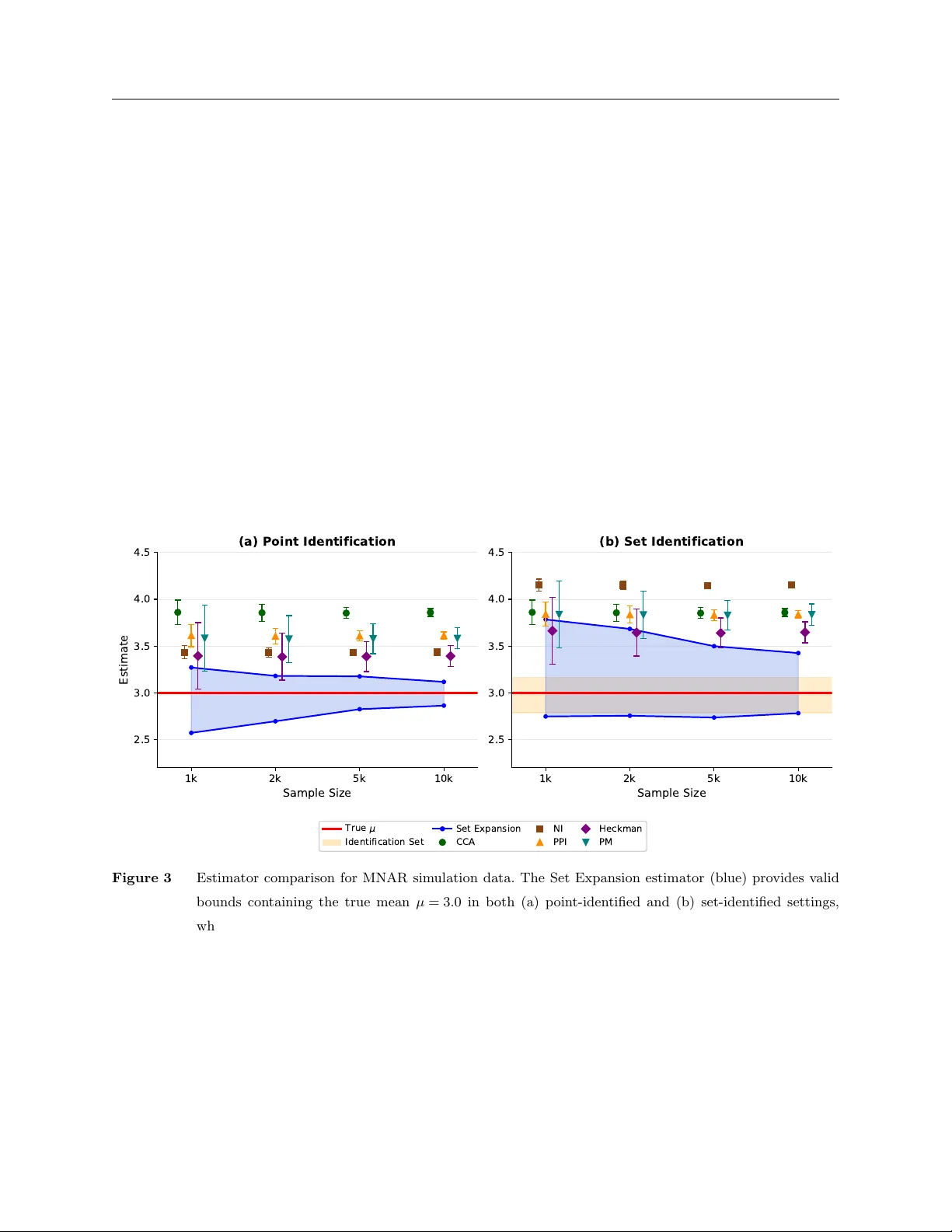
P artial Iden tiﬁcation under Missing Data Using W eak Shado w V ariables from Pretrained Mo dels Hongyu Chen 1 Da vid Simc hi-Levi 1 Ruo xuan Xiong 2 1 Massach usetts Institute of T echnology , Cam bridge, MA 02139 2 Emory Univ ersity , Atlan ta, GA 30322 chenhy@mit.edu, dslevi@mit.edu, ruoxuan.xiong@emory.edu Estimating p opulation quan tities such as mean outcomes from user feedback is fundamental to platform ev aluation and so cial science, yet feedback is often missing not at random (MNAR): users with stronger opinions are more likely to resp ond, so standard estimators are biased and the estimand is not iden tiﬁed without additional assumptions. Existing approaches typically rely on strong parametric assumptions or b esp ok e auxiliary v ariables that may be una v ailable in practice. In this pap er, w e dev elop a partial iden tiﬁ- cation framework in which sharp b ounds on the estimand are obtained by solving a pair of linear programs whose constraints encode the observ ed data structure. This formulation naturally incorporates outcome pre- dictions from pretrained models, including large language mo dels (LLMs), as additional linear constraints that tigh ten the feasible set. W e call these predictions we ak shadow variables : they satisfy a conditional inde- p endence assumption with resp ect to missingness but need not meet the completeness conditions required b y classical shadow-v ariable metho ds. When predictions are suﬃciently informative, the b ounds collapse to a point, recov ering standard identiﬁcation as a sp ecial case. In ﬁnite samples, to pro vide v alid co verage of the iden tiﬁed set, we propose a set-expansion estimator that ac hieves slo wer-than- √ n con vergence rate in the set-identiﬁed regime and the standard √ n rate under point identiﬁcation. In simulations and semi- syn thetic exp eriments on customer-service dialogues, we ﬁnd that LLM predictions are often ill-conditioned for classical shado w-v ariable metho ds yet remain highly eﬀective in our framework. They shrink iden tiﬁca- tion interv als by 75–83% while maintaining v alid cov erage under realistic MNAR mechanisms. Key wor ds : partial identiﬁcation; missing not at random; shado w v ariables; large language models; linear programming 1. Intro duction Missing data is p erv asive in economic and social researc h as well as on digital platforms. In house- hold and health surv eys, resp ondents often skip questions p erceiv ed as sensitiv e or irrelev an t. On digital platforms, users often choose whether or not to lea ve feedback based on their exp eriences. As noted b y Abrev ay a and Donald ( 2017 ), nearly 40% of top economics pap ers rep ort data miss- ingness, with ab out 70% dropping observ ations as a result. In man y of these settings, data is missing not at r andom (MNAR): the probabilit y of observing an outcome dep ends on its p ossibly unobserved v alue. F or example, Bollinger et al. ( 2019 ) sho ws that nonresp onse across the earnings distribution is U-shap ed, where left-tail “strugglers” and 1 2 Chen, Simchi-Levi, and Xiong: Partial Identiﬁc ation under MNAR Data righ t-tail “stars” are least likely to rep ort earnings. Conv ersely , an inv erse U-shap ed missingness pattern can b e found in online product reviews, where users with more extreme opinions are more lik ely to leav e reviews ( Hu et al. 2017 ). This dep endence b et w een missingness and actual outcome creates a fundamental c hallenge for accurate estimation and decision-making. Estimators based solely on observ ed data without modeling the missing mec hanism can b e severely biased, motiv ating approac hes that explicitly accoun t for the missingness mec hanism. In this pap er, we study the problem of iden tifying p opulation quan tities, suc h as the mean outcomes, when data are MNAR. Such questions are prev alent in service platforms or so cial surv eys, e.g., when a platform seeks to ev aluate av erage customer satisfaction, or when a researcher aims to estimate a verage income in a particular region. F or those questions, one class of classical metho ds addresses this MNAR problem by imp osing strong parametric structural assumptions, suc h as those in the Heckman selection mo del ( Hec kman 1979 ) or the P attern-Mixture mo del ( Rubin 1987 , Little 1994 ). Another common approach introduces auxiliary v ariables, including instrumen tal v ariables ( d’Haultfo euille 2010 ) or shadow v ariables ( Miao and Tchetgen Tc hetgen 2016 ), whic h need to satisfy restrictive indep endence or completeness conditions for identiﬁcation. Both strategies can face practical limitations: structural parametric models ma y be missp eciﬁed, and iden tifying v alid auxiliary v ariables ma y require substantial domain expertise or serendipity . W e therefore take a diﬀeren t approach and study: under realistically minimal assumptions, what can we still learn about p opulation quantities lik e the mean outcomes? Instead of seeking p oint iden tiﬁcation, w e adopt a partial iden tiﬁcation p ersp ective ( Manski 2003 ) and aim to c haracterize sharp upp er and lo wer b ounds on the estimand (e.g., mean outcome). Our key insight is that this problem can b e reformulated as a pair of linear programs (LPs). In this form ulation, the ob jective corresp onds to the estimand, while constrain ts enco de the probabilistic structure implied by the observ ed data. This yields a transparen t and tractable framew ork for estimation under MNAR. While b ounds obtained under minimal assumptions are v alid, they can b e wide, especially when a large p ortion of the data is missing. T o tighten the b ounds, we prop ose incorp orating auxiliary predictions from mo dern machine learning systems, such as large language mo dels (LLMs). Recent w ork suggests that LLMs exhibit h uman-lik e reasoning abilities and can approximate decision- making in complex settings ( Horton 2023 , Goli and Singh 2024 , Brand et al. 2024 ), making them promising candidates for predicting unobserved outcomes, e.g. predicting user satisfaction from c hat transcripts. Imp ortantly , b ecause suc h predictions are generated by an external mo del rather than b y the individuals themselves, they do not directly inﬂuence whether an outcome is observ ed; that is, they naturally satisfy an exclusion-type condition with resp ect to the missingness mechanism. A t the same time, discrepancies b etw een LLM outputs and actual h uman b eha vior ha ve been do cumen ted ( Gui and T oubia 2023 , Li et al. 2024 , Gao et al. 2025 ), and researchers ha ve cautioned Chen, Simchi-Levi, and Xiong: Partial Identiﬁc ation under MNAR Data 3 against assuming that mo del predictions can p erfectly substitute for h uman judgments. These observ ations suggest that LLM predictions can serv e as useful auxiliary signals for tigh tening iden tiﬁcation b ounds, but that an approach robust to prediction imp erfections is needed. In light of b oth the promise and limitations of these predictions, w e treat LLM-generated outputs as we ak shadow variables . Sp eciﬁcally , w e assume an exclusion-t yp e condition: conditional on the true outcome and observ ed cov ariates, the prediction is indep enden t of the missingness indicator. Ho w ev er, w e do not require strong relev ance or completeness conditions as in classical shadow v ariables ( Miao and Tc hetgen Tc hetgen 2016 ); the predictions ma y only weakly correlate with the outcome. Even so, incorp orating them introduces additional linear constraints in to our identiﬁca- tion framework, tigh tening the feasible region. When the predictions are suﬃcien tly informative, the b ounds may collapse to a single p oint, yielding point iden tiﬁcation as a sp ecial case. 1.1. Main Contributions W e summarize our three main con tributions b elo w. First, we prop ose a nov el linear programming framework for partial identiﬁcation under MNAR that applies both with and without auxiliary predictions. In the baseline setting without auxil- iary inputs, the formulation yields closed-form solutions for the iden tiﬁcation region of the mean outcomes. When incorp orating auxiliary predictions from LLMs, w e deriv e analytical results that quan tify how these predictions tigh ten the feasible set and shrink the identi ﬁcation region. This form ulation oﬀers a uniﬁed and tractable approach to understanding ho w predictive signals impact iden tiﬁcation under minimal assumptions. Second, we dev elop a set-expansion estimator that asymptotically conv erges to the identiﬁcation region while accounting for estimation error in the probability constraints that deﬁne the bounds. W e establish conv ergence rates for this estimator. In the partially identiﬁed setting, the con vergence rate is slow er than the usual √ n rate (for example, on the order of √ n/ log n ), as a result of the additional uncertaint y inheren t in set identiﬁcation. When the auxiliary information is suﬃciently informativ e and p oint identiﬁcation is ac hieved, the estimator recov ers the standard √ n rate, matc hing classical results in the shadow v ariable literature ( Miao and Tchetgen Tchetgen 2016 ). W e further extend our framework to randomized experiments and deriv e b ounds on treatment eﬀects, and provide suﬃcien t conditions under which reliable treatment decisions can still b e made despite missing outcomes. Third, w e ev aluate the prop osed metho ds through sim ulation studies and semi-syn thetic exp er- imen ts based on real customer-service dialogue data. T o construct auxiliary signals, we generate outcome predictions using LLMs under several prompting and training regimes, including zero- shot, few-shot, c hain-of-though t prompting, and ﬁne-tuning. Our results reveal tw o key insights. 4 Chen, Simchi-Levi, and Xiong: Partial Identiﬁc ation under MNAR Data First, w e show that LLM predictions can fail to meet the strong completeness conditions required for classical shadow v ariable metho ds, rendering p oint iden tiﬁcation unstable or infeasible. This underscores the need for our partial identiﬁcation framework. Second, despite these limitations, the predictions remain informative: incorp orating LLM-based weak shado w v ariables reduces the width of iden tiﬁcation interv als by 75–83% across prompting strategies, while preserving v alid cov erage under realistic MNAR mec hanisms. 1.2. Related W o rk Our w ork con tributes to the rich literature on iden tiﬁcation and estimation under MNAR mec ha- nisms. Classical approac hes include parametric selection mo dels, such as the Heckman correction, whic h join tly mo dels the outcome and missingness process ( Heckman 1979 ), and Pattern-Mixture mo dels that parameterize outcome distributions within eac h missingness stratum ( Little 1994 , Rubin 1987 ). Other strands of w ork lev erage graphical mo dels to represent missing data pro cesses ( F a y 1986 ), or use auxiliary v ariables such as instrumen tal v ariables that aﬀect missingness but not outcomes ( Das et al. 2003 , Tchetgen Tc hetgen and Wirth 2017 , Sun et al. 2018 ). Our approach is most closely aligned with recent developmen ts in the shado w v ariable literature ( d’Haultfo euille 2010 , Miao and Tchetgen Tc hetgen 2016 , Miao et al. 2024 ), which t ypically uses the o dds ratio for the iden tiﬁcation of the distribution of missing outcomes. W e con tribute to this line of researc h in three key wa ys. First, we in tro duce a nov el linear programming framework that characterizes the iden tiﬁcation region for mean outcomes under MNAR. Second, we generalize the shado w v ariable approac h b y allo wing weak shadow v ariables; this enables the use of auxiliary signals, e.g., from LLMs, that may violate classical completeness assumptions and th us do not yield p oint iden ti- ﬁcation but can still signiﬁcan tly tighten bounds. Third, we establish con vergence rates for our estimated iden tiﬁcation region under b oth partial and p oint identiﬁcation regimes. Our linear programming formulation connects to the broader literature on inference for partially iden tiﬁed mo dels ( Manski 2003 , Im b ens and Manski 2004 ). Chernozh uko v et al. ( 2007 ) proposed a criterion-function approac h with set expansion to construct conﬁdence regions for identiﬁed sets, whic h directly inspires our estimator. Bereste an u and Molinari ( 2008 ) connect identiﬁed sets to LP optimal v alues through a support function characterization, and Mogstad et al. ( 2018 ) and Kaido et al. ( 2019 ) dev elop LP-based inference for treatmen t eﬀect b ounds and subv ector pro jections, resp ectiv ely . Our work de riv es a speciﬁc LP structure from the shado w v ariable assumption under MNAR and shows that auxiliary predictions generate additional constraints that tigh ten the iden- tiﬁed set, with conv ergence rates that adapt to whether the shadow v ariable yields partial or p oint iden tiﬁcation. Chen, Simchi-Levi, and Xiong: Partial Identiﬁc ation under MNAR Data 5 Our w ork also relates to the gro wing literature on leveraging pretrained mo dels as auxiliary signals to impro ve identiﬁcation or statistical eﬃciency . Prediction-pow ered inference (PPI) meth- o ds ( Angelop oulos et al. 2023a , b ) assume true labels are observ ed for only a random subset of the data, when predictions from an external model are av ailable for the remainder, and aim to com bine the t wo sources to enable v alid inference. Ji et al. ( 2025 ) prop ose PPI with “recalibrated” prediction, learning a map from the mo del prediction and cov ariates to the true outcome to correct bias. W ang et al. ( 2025 ) further prop ose optimal sample allo cation strategies that ﬁrst ﬁne-tune LLMs and then apply PPI to correct for prediction bias. F rom a diﬀerent p ersp ective, W ang et al. ( 2024 ) explore how LLM-generated simulations, when grounded in real data, can supp ort accurate conjoin t analysis. Chen et al. ( 2025 ) further examine how to design data collection and eﬃcien t inference strategies in the presence of suc h LLM-based predictors. Our w ork diﬀers in t wo key w a ys. First, we explicitly account for MNAR missingness. Second, w e interpret auxiliary predic- tions as weak shadow v ariables, leading to a framework that pro vides v alid b ounds on p opulation quan tities, rather than relying on p oint estimates that require stronger missingness assumptions. The remainder of the pap er is organized as follows. Section 2 introduces the problem setup. Sec- tion 3 dev elops the linear programming framework for partial identiﬁcation, both with and without w eak shadow v ariables. Section 4 presents the set-expansion estimator and its con v ergence prop- erties. Section 5 extends the framework to randomized exp eriments. Section 6 rep orts sim ulation and semi-syn thetic exp eriments, and Section 7 concludes. 2. Problem Setup Supp ose w e are ev aluating an economic, so cial, or digital system that solicits discrete feedback, suc h as surv ey resp onses, program satisfaction ratings, or customer-service reviews on online plat- forms. Outcomes are observed only when individuals c ho ose to respond. Because not all individuals pro vide feedback, outcomes are partially observed. Let R ∈ { 0 , 1 } indicate whether a user’s rating is observed ( R = 1) or missing ( R = 0). The rating is denoted by Y ∈ [ M ], where [ M ] = { 1 , . . . , M } represen ts a discrete set of p ossible scores. W e fo cus on the setting where the missingness is not at random, meaning that the probability of observing a rating may dep end on its v alue, that is, R ⊥ ⊥ Y . This is motiv ated by empirical evidence that users with extreme, either p ositive or negative, ratings are more likely to write reviews than users with mo derate pro duct ratings ( Hu et al. 2017 ). Thus, our observ ation is a set of i.i.d. data { R i , R i Y i } n i =1 with Y i observ ed if and only if R i = 1, and n is the num b er of observ ations. Our primary ob jectiv e is to estimate the mean outcome θ = E [ Y ] 6 Chen, Simchi-Levi, and Xiong: Partial Identiﬁc ation under MNAR Data suc h as the av erage rating across all customers. While w e fo cus on the p opulation mean for con- creteness, our framework extends directly to other p opulation quan tities, including functionals of the form E [ g ( Y )] and other distributional summaries, as discussed later. Ho w ev er, when outcomes are missing not at random, the observed ratings ma y not represent the full p opulation, and a naive empirical a verage ov er observ ed data is typically biased. As a result, p oin t identiﬁcation of θ is generally infeasible without additional assumptions on the missingness mec hanism, e.g., via in tro ducing additional v ariables or a parametric mo del on missing pattern ( Hec kman 1979 , Little 1994 ). These underlying structural assumptions are generally un testable from observed data and may also lead to biased estimates. In this pap er, we study this problem in a fully non-parametric w ay with minimal structural assumptions. In particular, we adopt a partial iden tiﬁcation p ersp ectiv e: rather than aiming for a single estimate under ten uous assumptions, we c haracterize the range of v alues θ can plausibly tak e given the observ ed data. 3. P artial Identiﬁcation via Linear Programs In this section, w e dev elop a linear-programming c haracterization of partial identiﬁcation under MNAR. W e ﬁrst sho w that the sharp iden tiﬁcation set for the estimand θ reduces to an explicit in terv al whose endpoints solve a simple pair of linear programs. W e then sho w how predictions from a pretrained mo del can b e incorporated as weak shadow v ariables and yield additional linear constrain ts to tigh ten the iden tiﬁcation set. 3.1. P artial Identiﬁcation in the Base Case Our partial identiﬁcation strategy is based on the follo wing decomp osition of the p opulation mean: θ = M X y =1 y · P ( Y = y ) = M X y =1 y · P ( Y = y , R = 1) | {z } := α ( y )  P ( R = 1 | Y = y ) | {z } := π ( y ) . If we are interested in other population quantities (e.g., E [ g ( Y )]), then w e replace y · P ( Y = y ) b y g ( y ) · P ( Y = y ) in the decomp osition. Here, the joint probabilit y α ( y ) = P ( Y = y , R = 1) is iden tiﬁable from observed data. How ever, the conditional resp onse probabilit y π ( y ) = P ( R = 1 | Y = y ) is generally unidentiﬁable when missingness dep ends on the outcome itself. As a result, the mean θ cannot b e p oint-iden tiﬁed without further assumptions. W e c haracterize the sharp identiﬁcation region for θ b y considering all possible v alues of π ( y ) ∈ (0 , 1]. Note that the only constrain t from observ ational data is that the probabilities P ( Y = y ) must sum to one. Th us, w e can deﬁne the feasible set for π ( y ) as: Π = ( ( π (1) , . . . , π ( M )) : M X y =1 α ( y ) /π ( y ) = 1 , π ( y ) ∈ (0 , 1] ) . Chen, Simchi-Levi, and Xiong: Partial Identiﬁc ation under MNAR Data 7 This induces the iden tiﬁcation set for the mean outcome: Θ = ( M X y =1 y · α ( y ) /π ( y ) : ( π ( y )) y ∈ [ M ] ∈ Π ) . T o simplify notations, let w ( y ) = 1 /π ( y ) − 1. Under this change of v ariables, the feasible region b ecomes a p olyhedron in w ( y ), and the mapping from w ( y ) to θ is linear. Th us, the identiﬁcation region Θ is a closed in terv al, and its endp oints can b e computed b y solving the follo wing pair of linear programs: θ min = min w ( y ) M X y =1 y · α ( y )( w ( y ) + 1) s.t. M X y =1 α ( y )( w ( y ) + 1) = 1 w ( y ) ≥ 0 ∀ y θ max = max w ( y ) M X y =1 y · α ( y )( w ( y ) + 1) s.t. M X y =1 α ( y )( w ( y ) + 1) = 1 w ( y ) ≥ 0 ∀ y (1) Therefore, the iden tiﬁed region for the mean outcome is giv en by Θ = [ θ min , θ max ]. In the propo- sition b elo w, we show that both θ min and θ max can b e solved analytically . Proposition 1. The sharp identiﬁc ation r e gion for θ given observe d MNAR data { R i , R i Y i } n i =1 is Θ = [ θ min , θ max ] deﬁne d in ( 1 ) , which has close d-form solutions: θ min = P ( R = 1) E [ Y | R = 1] + P ( R = 0) θ max = P ( R = 1) E [ Y | R = 1] + M · P ( R = 0) . Here w e implicitly let P ( R = 1) E [ Y | R = 1] b e zero if P ( R = 1) is zero and hence E [ Y | R = 1] is undeﬁned. These expressions are attained by setting the weigh ts w ( y ) to their minimum allow able v alue w ( y ) = 0 for all but one outcome level. T o ac hieve θ min , w e set w ( y ) = 0 for y = 2 , . . . , M and assign the remaining mass to y = 1, the smallest outcome. Conv ersely , to ac hieve θ max , w e set w ( y ) = 0 for y = 1 , . . . , M − 1 and concentrate the remaining w eight on y = M , the largest outcome. This corresponds to placing as muc h probabilit y mass as p ossible on the lo west or highest feasible rating lev els, sub ject to the constrain t induced by the observ ed joint distribution α ( y ) = P ( Y = y , R = 1). Notably , the width of the iden tiﬁcation region is θ max − θ min = ( M − 1) · P ( R = 0), which scales linearly with the probability of missingness. When P ( R = 0) = 0, i.e., outcomes are fully observ ed, the b ounds collapse to a point and θ is point-iden tiﬁed. In con trast, when P ( R = 0) = 1, the b ounds are equal to the full supp ort range, [1 , M ], which is uninformative. Without additional information and structural assumptions, the iden tiﬁcation region in Proposition 1 is the best one can hop e for. They are sharp bounds for iden tiﬁcation in the sense that any other v alid identiﬁcation region from observ ed data will con tain Θ as a subset. 8 Chen, Simchi-Levi, and Xiong: Partial Identiﬁc ation under MNAR Data 3.1.1. Extension to the Case with Co v ariates In many applications, additional co v ariates are av ailable. F or example, online platforms and social science studies often collect structured demographic information such as age, race, or lo cation, and a common practice is to stratify analyses across suc h cov ariate groups to reduce heterogeneity and improv e precision. Motiv ated b y this, w e study how the inclusion of cov ariates aﬀects the identiﬁcation region Θ. T o build in tuition, w e focus on the setting where co v ariates take on ﬁnitely many v alues and can b e stratiﬁed in to discrete groups, although the same ideas can extend to contin uous cov ariates. Let X ∈ X = { x 1 , . . . , x K } and consider stratifying the analysis b y each co v ariate level. The mean outcome can b e decomp osed as θ = X x ∈X M X y =1 y · P ( Y = y , R = 1 | X = x ) P ( R = 1 | Y = y , X = x ) P ( X = x ) . Under the same pro cedure, we can derive a sharp iden tiﬁcation region for the target v ariable θ . Proposition 2. When we include c ovariates, the sharp identiﬁc ation r e gion for θ c oincides with that obtaine d without c ovariates. In p articular, the identiﬁc ation b ounds on θ under str atiﬁc ation have the fol lowing close d-form solutions: θ strat min = X x ∈X [ P ( R = 1 | X = x ) E [ Y | R = 1 , X = x ] + P ( R = 0 | X = x ) ] P ( X = x ) = θ min θ strat max = X x ∈X [ P ( R = 1 | X = x ) E [ Y | R = 1 , X = x ] + M · P ( R = 0 | X = x ) ] P ( X = x ) = θ max . In terestingly , these b ounds coincide exactly with those obtained from the unstratiﬁed form ula- tion. Hence, stratifying on cov ariates do es not tighten the iden tiﬁcation region. Intuitiv ely , this is b ecause the e xtreme mass allo cations (to outcome y = 1 or y = M ) are feasible within eac h stra- tum indep endently and carry through under marginalization. This motiv ates the necessity of extra v ariables with richer structural prop erties for sharp er iden tiﬁcation. In the next section, we will consider additional predictions as a co v ariate that satisfy a conditional indep endence structure. Under that scenario, w e will observ e a sharp ened identiﬁcation region. 3.2. Leveraging Pretrained Foundation Mo dels to Reﬁne Identiﬁcation Bounds In many mo dern settings, w e hav e access to rich unstructured data, such as chat transcripts, reviews, or other in teraction logs, that plausibly enco de information ab out the missing outcomes. Directly incorp orating such high-dimensional inputs in to stratiﬁed analyses is typically infeasible. Instead, w e propose to lev erage pretrained foundation models to extract low-dimensional predictive signals from these data. In particular, w e feed them in to a pretrained mo del (e.g., an LLM) to pro duce an output F ∈ F that serv es as a pro xy for how a human would rate the interaction, thereb y injecting additional information ab out the latent outcome distribution. In practice, w e Chen, Simchi-Levi, and Xiong: Partial Identiﬁc ation under MNAR Data 9 can prompt the mo del to return a discrete rating (e.g., “c ho ose one of { 1 , . . . , M } ”), so F is ﬁnite and, without loss of generalit y , w e can tak e F = [ M ] to matc h the supp ort of Y . W e assume F is alwa ys observed along with additional co v ariates X . Thus, the ﬁnal dataset tak es the form { F i , X i , R i , R i Y i } n i =1 . W e impose the following assumption on the relationship b et w een the model output and the missingness mec hanism: Assumption 1 (W eak Shadow V ariable) . The mo del output F is c onditional ly indep endent of the missingness indic ator R given the true outc ome Y and c ovariates X , i.e., F ⊥ ⊥ R | Y , X . W e call F a We ak Shadow V ariable if it satisﬁes Assumption 1 and its connection to classic shado w v ariable will be clear in the next section. This is a relatively w eak assumption that do es not require the predictive mo del to b e accurate. It states that, once w e condition on the actual outcome and co v ariates, the model output pro vides no additional information about whether the outcome is observ ed. This condition holds in most applications, as users’ decisions to resp ond typically do not dep end on an external predictor that they never observe. As a sanity chec k, if the prediction is p erfect, i.e., F = Y , then Assumption 1 is trivially satis ﬁed. A causal diagram for the relationship can b e found in Figure 1 . 3.2.1. Connection to the Shadow V ariable F ramew ork Assumption 1 is closely related to the shadow variable/auxiliary variable framew ork, which has been proposed as an alternativ e to instrumen tal v ariable approac hes in the literature on nonrandom missing data ( Miao and Tc h- etgen Tchetgen 2016 , Miao et al. 2024 ). In this section, we clarify our connections and ho w our deﬁnition for w eak shado w v ariable generalizes the traditional approac h. Definition 1 (Shadow V ariable). A v ariable F is fully observ ed and is called a shadow v ari- able if it satisﬁes: (i) F is asso ciated with the outcome Y , i.e., F ⊥ ⊥ Y | X , R = 1; and (ii) F do es not directly aﬀect the selection mec hanism, i.e., F ⊥ ⊥ R | Y , X . The shadow v ariable framework provides a pathw ay to handle MNAR data and has been widely adopted in empirical studies ( Ibrahim et al. 2001 , Kott and Liao 2018 ). Ho w ev er, the existence of a shado w v ariable alone is not suﬃcient for p oint iden tiﬁcation of the estimand θ . In addition to the tw o conditions in Deﬁnition 1 , prior work requires c ompleteness of the conditional distribution P ( Y | R = 1 , X, F ) as another constraint to ensure p oint identiﬁcation ( Miao and Tchetgen Tc hetgen 2016 , Miao et al. 2024 ). Definition 2 (Completeness of P ( Y | X , F , R = 1) ). F or a shado w v ariable F , the conditional distribution P ( Y | X , F , R = 1) is called complete if, for each x , for all square-integrable functions h ( x, Y ), E [ h ( x, Y ) | X = x, F , R = 1] = 0 almost surely implies h ( x, Y ) = 0 almost surely . 10 Chen, Simchi-Levi, and Xiong: Partial Identiﬁc ation under MNAR Data X R Y F Figure 1 Causal diagram depicting the relationships among observed co v ariates X , true outcome Y , observ a- tion indicator R , and predicted outcome F . W e assume conditional independence F ⊥ ⊥ R | Y , X . The dashed arrow from F to Y indicates an optional dep endence; we do not require the full shadow v ariable assumption. The completeness condition is a strengthened v ersion of the dep endence constraint in Deﬁni- tion 1 —not only must the shadow v ariable F and the outcome Y b e dep endent, but the v ariation in F m ust b e suﬃcient to explain the v ariation in Y . Under our discrete outcome setup, the completeness condition admits a cleaner in terpretation in terms of matrix algebra. Deﬁne the join t distribution matrix H = [ P ( F = f , Y = y )] f ∈F ,y ∈ [ M ] ∈ R |F |× M and the conditional distribution matrix B = [ P ( Y = y | F = f , R = 1)] f ∈F ,y ∈ [ M ] ∈ R |F |× M . Note that H is indep endent of the miss- ingness scheme but B is related to the distribution of R . Completeness then corresp onds directly to a full-rank condition on the matrix B , which is further equiv alen t to a rank condition on H under mild assumptions. Proposition 3. F or discr ete outc omes Y and a shadow variable F , the c ompleteness c ondition holds if and only if rank( B ) = M . F urthermor e, if π ( y ) ∈ [ π , π ] and P ( F = f , R = 1) ∈ [ p F , p F ] for strictly p ositive c onstants π and p F for al l y and f , then the c ompleteness c ondition is e quivalent to rank( H ) = M , and the c ondition numb ers satisfy κ ( B ) ≤ p F p F · π π · κ ( H ) . Prop osition 3 translates the abstract completeness condition into a concrete matrix rank con- dition, whic h is muc h simpler to interpr et and v erify in practice. The condition n umber κ ( H ) quan tiﬁes the degree of in vertibilit y of the joint distribution matrix: when κ ( H ) is close to one, the matrix is w ell-conditioned and completeness holds strongly; when κ ( H ) is large, the matrix is nearly rank-deﬁcien t and completeness barely holds. W e will use H rather than B to ev aluate the prediction in later exp eriment section as it do es not dep end on the missingness sc heme. P oin t identiﬁcation using shadow v ariables relies on solving a F redholm integral equation, whose n umerical stabilit y dep ends critically on the condition n umber of matrix B . In modern applications where predictiv e mo dels are generic rather than problem-sp eciﬁc—as is the case with large language mo dels—the predictions may not fully capture v ariation in the outcome, resulting in ill-conditioned Chen, Simchi-Levi, and Xiong: Partial Identiﬁc ation under MNAR Data 11 matrices H and, by Prop osition 3 , ill-conditioned matrices B . As we demonstrate in Section 6 , LLM-generated predictions for real customer service data yield condition num b ers on the order of 10 3 and minim um singular v alues around 10 − 4 , rendering p oin t iden tiﬁcation numerically unstable. Our deﬁnition of a w eak shadow v ariable departs from the classical shadow v ariable literature in an imp ortan t wa y: w e fully relax b oth the dep e ndence and completeness conditions. W e show that neither condition is necessary to iden tify bounds on θ . Moreo ver, the prop osed iden tiﬁca- tion b ounds adapt naturally to the strength of correlation b etw een Y and F conditional on X and R = 1. Stronger correlation leads to tighter identiﬁcation regions, and completeness recov ers p oin t identiﬁcation as a limiting case. Another adv an tage of the partial identiﬁcation approac h is computational: rather than solving potentially ill-conditioned integral equations, we solv e a lin- ear program with relaxed constrain ts, whic h is numerically more stable. This p ersp ective allo ws practitioners to leverage mo dern predictive mo dels as auxiliary to ols for tightening identiﬁcation regions without imp osing stringent requirements on predictiv e accuracy . 3.2.2. Iden tiﬁcation Region In this section, w e pro ceed to develop the sharp iden tiﬁcation region for θ with w eak shado w v ariables. Here our partial iden tiﬁcation strategy is based on strat- iﬁcation θ = P x ∈X θ x · P ( X = x ), where θ x = E [ Y | X = x ] is the conditional mean within stratum x . W e will ﬁrst pro vide an identiﬁcation region for ev ery x ∈ X and then aggregate them together to obtain an iden tiﬁcation region for θ . F or eac h x ∈ X , we ha ve the follo wing decomp osition θ x = X f ∈F M X y =1 y · P ( F = f , Y = y | X = x ) = X f ∈F M X y =1 y · P ( R = 1 , F = f , Y = y | X = x ) | {z } := α x ( f ,y )  P ( R = 1 | F = f , Y = y , X = x ) | {z } := π x ( y ) . The second equalit y follows from the chain rule of probabilit y . Under Assumption 1 , i.e., F ⊥ ⊥ R | Y , w e ha v e P ( R = 1 | Y = y , X = x ) = P ( R = 1 | F = f , Y = y , X = x ) for all f ∈ F , so the denominator do es not dep end on f . W e therefore write it as π x ( y ) for notation simplicity . The quan tity α x ( f , y ) is iden tiﬁable from observ ed data, but π x ( y ) remains unidentiﬁable. W e therefore propose to iden tify a set of feasible v alues for π x ( y ). Here, w e leverage the following iden tit y: P ( R = 0 , F = f | X = x ) | {z } := β x ( f ) = M X y =1 P ( R = 0 , F = f , Y = y | X = x ) = M X y =1 P ( F = f , Y = y | X = x ) P ( R = 0 | Y = y , X = x ) = M X y =1 α x ( f , y ) π x ( y ) · (1 − π x ( y )) 12 Chen, Simchi-Levi, and Xiong: Partial Identiﬁc ation under MNAR Data where the second equality uses Assumption 1 . W e let β x ( f ) = P ( R = 0 , F = f | X = x ) for notation simplicit y . Note that β x ( f ) is iden tiﬁable from observ ed data. Thus, for eac h x ∈ X , we can similarly write the feasible region for π x ( y ) as Π x = ( ( π x (1) , . . . , π x ( M )) : M X y =1 α x ( f , y )  1 π x ( y ) − 1  = β x ( f ) , ∀ f ∈ F , π x ( y ) ∈ (0 , 1] ) and the iden tiﬁcation region for θ x b ecomes Θ x = ( X f ∈F M X y =1 y α x ( f , y ) π x ( y ) : ( π x ( y )) y ∈ [ M ] ∈ Π x ) . Letting w x ( y ) = 1 /π x ( y ) − 1, we obtain a linear represen tation of the ob jective and constrain ts in terms of w x ( y ). The feasible set Π x remains con vex, and so the iden tiﬁcation region Θ x is a closed in terv al. The endp oin ts are giv en b y the solution to the follo wing pair of linear programs: θ x, min = min w x 1 ⊤ A x D ( w x + 1 ) s.t. A x w x = β x w x ≥ 0 θ x, max = max w x 1 ⊤ A x D ( w x + 1 ) s.t. A x w x = β x w x ≥ 0 (2) where A x = [ α x ( f , y )] f ,y ∈ [0 , 1] |F |× M , w x = ( w x (1) , . . . , w x ( M )) ⊤ , and β x = ( β x (1) , . . . , β x ( |F | )) ⊤ , D = diag { 1 , 2 , . . . , M } , and 1 and 0 are vectors of all ones and zeros, resp ectively . The constrain ts here restrict π x ( y ) to lie in Π x where the ob jective function is the deﬁnition of θ ∈ Θ x . Aggregating o v er co v ariate strata, w e obtain the sharp identiﬁcation region for the estimand θ . Proposition 4. Under Assumption 1 , the sharp identiﬁc ation r e gion for θ is given by Θ = " X x ∈X θ x, min · P ( X = x ) , X x ∈X θ x, max · P ( X = x ) # :=  θ shad min , θ shad max  . wher e θ x is deﬁne d in ( 2 ) . Mor e over, θ is p oint identiﬁe d if A x has ful l c olumn r ank for al l x ∈ X . The iden tiﬁcation of θ depends on the identiﬁcation of eac h stratum mean θ x , whic h in turn is gov erned by the linear system A x . If A x has full column rank, i.e., rank( A x ) = M , then it corresp onds to the completeness condition in Deﬁnition 2 . In this scenario, the linear constraint system has a unique solution, and we achiev e p oint identiﬁcation: θ x, min = θ x, max . More generally , if some ro ws of A x are linearly dep enden t (e.g., F ⊥ ⊥ Y | X , R = 1 for every F ∈ F ′ for some subset F ′ ⊂ F ) or if the columns are dep endent (e.g., F ⊥ ⊥ Y | X , R = 1 for a subset of outcomes Y ∈ Y ′ ⊂ { 1 , . . . , M } ), then the feasible region contains m ultiple solutions and w x is only partially identiﬁed. In this sense, our form ulation generalizes the classical shado w v ariable approac h: it allo ws violations of the completeness condition of the shado w v ariable deﬁnition and quan titativ ely c haracterizes ho w the strength of asso ciation b etw een F and Y impacts the width of the iden tiﬁcation region Θ x . Chen, Simchi-Levi, and Xiong: Partial Identiﬁc ation under MNAR Data 13 Again, the iden tiﬁcation in Prop osition 4 is sharp in the sense that any other v alid identiﬁcation region based on the observ ed data will con tain [ θ shad min , θ shad max ] as a subset. Lastly , w e compare the ab o ve iden tiﬁcation region with the one deﬁned in Equation ( 1 ) where the shadow v ariable is not av ailable to understand the eﬀect of the additional prediction F . Note that the formulation in linear program ( 2 ) is closely related to linear program ( 1 ), where the constrain t for the low er b ound in linear program ( 1 ) can b e written as a single aggregated constraint 1 ⊤ A x w x = 1 ⊤ β x . Thus, we can use the techniques in aggregation b ounds ( Zipkin 1980 , Litvinchev and Tsurk o v 2013 ) to analyze their diﬀerences. Theorem 1. Write matrix A x = [ a x, 1 , a x, 2 , . . . , a x,M ] , we have θ max − θ shad max ≥ X x ∈X 1 ⊤ β x 2     β x 1 ⊤ β x − a x,M 1 ⊤ a x,M     1 · P ( X = x ) ≥ 0 , θ shad min − θ min ≥ X x ∈X 1 ⊤ β x 2     β x 1 ⊤ β x − a x, 1 1 ⊤ a x, 1     1 · P ( X = x ) ≥ 0 . Theorem 1 giv es a c haracterization of the diﬀerence b etw een the identiﬁcation b ound with and without a shadow v ariable. The pro of is pro vided in App endix B.2 . As a sp ecial case, we ha ve the iden tiﬁcation with shadow v ariable is never worse than that without it, i.e., θ min ≤ θ shad min ≤ θ shad max ≤ θ max . Moreov er, the amount of impro vemen t dep ends on the missingness ratio (represen ted b e 1 ⊤ β x ) and the worst misalignment b et w een missingness data distribution and observed data distribution (c haracterized by    β x 1 ⊤ β x − a x,M 1 ⊤ a x,M    1 ). Th us, the shadow v ariable is especially useful when missingness lev el is high and when the missingness sc heme does not align well with observ ed sc heme, in whic h case the data is far from MAR. 4. Set Expansion Estimato r in Finite Samples In practice, when solving the linear programs in Equation ( 2 ), w e do not hav e access to the true probabilit y quantities A x = [ α x ( f , y )] f ,y and probabilit y vector β x = [ β x ( f )] f . Instead, w e estimate them from observ ed data and then solv e the optimization problem using the estimates to obtain ˆ θ x, min and ˆ θ x, max . This ma y cause problems as the system of linear equations may b e o v er-iden tiﬁed, resulting in unstable ﬁnite sample p erformance. In this section, we prop ose a set expansion estimator that ensures the solution from the linear program in ﬁnite sample is a v alid estimation for the estimand. Let D = { ( X i , R i , R i Y i , F i ) } n i =1 denote a random sample of size n , and let n x denote the n umber of units in stratum x , i.e., n x = P n i =1 1 ( X i = x ). W e assume that the estimators for α x ( f , y ) and β x ( f ) con v erge at the √ n x rate, as formalized in the assumption b elow. 14 Chen, Simchi-Levi, and Xiong: Partial Identiﬁc ation under MNAR Data Assumption 2. We assume the estimators ˆ A x and ˆ β x c onver ge at √ n x r ate for al l x , i.e., max f ,y | ˆ α x ( f , y ) − α x ( f , y ) | = O p  n − 1 / 2 x  , max f | ˆ β x ( f ) − β x ( f ) | = O p  n − 1 / 2 x  . This assumption is mild and holds under standard empirical or maxim um lik eliho o d estimators, giv en the ﬁnite supp ort of b oth f and y . Giv en the estimators ˆ A x and ˆ β x , a natural approach is to plug them into the LP formulation and solve the empirical analog of ( 2 ). Ho wev er, this direct plug-in metho d can lead to infeasibilit y or unstable solutions. This is b ecause the matrix A x ma y hav e linearly dep endent ro ws (dep ending on the informativ eness of F ), so even small estimation errors may p erturb the feasible region in a w a y that makes the empirical LP infeasible, ev en though the p opulation LP has a v alid solution. T o address this issue and ensure w ell-p osed optimization, we introduce a b ounded constraint on the solution space: Assumption 3. We assume ther e exists a known C > 0 such that the true solution w x ( y ) ∈ [0 , C ] for the line ar pr o gr am ( 2 ) for y ∈ [ M ] . This b oundedness assumption equiv alently implies a low er b ound on the conditional observ ation probabilit y: π x ( y ) = P ( R = 1 | Y = y , X = x ) ≥ 1 / ( C + 1). Suc h p ositivity conditions are standard in the missing data literature. Without suc h a lo w er bound, estimation of the outcome distribution for rarely observed strata b ecomes ill-p osed, as there would be insuﬃcient information in the observed data to learn ab out the missing v alues. Next, we prop ose to use a set expansion approac h, inspired by Chernozh uk o v et al. ( 2007 ), to ensure that the empirical analog of ( 2 ) remains feasible even when using the estimators ˆ A x and ˆ β x . Sp eciﬁcally , we quantify the violation of estimated linear constrain ts within the b ounded solution space b y computing the follo wing diagnostic: ˆ m x = min 0 ≤ w x ≤ C ∥ ˆ A x w x − ˆ β x ∥ ∞ . This quantit y captures the minimax deviation from the constraint ˆ A x w x = ˆ β x o v er all candidate solutions within the b ounded region 0 ≤ w x ≤ C . Intuitiv ely , ˆ m x measures the degree of infeasibility in tro duced by the estimation error. If the empirical linear program is exactly feasible, then ˆ m x = 0; otherwise, ˆ m x > 0 reﬂects the minimal slack needed to make the LP feasible again. Using ˆ m x and a user-speciﬁed tolerance sequence κ n x > 0, w e deﬁne the set expansion estimator of θ x, min as the solution to the follo wing relaxed linear program: ˆ θ x, min = min w x 1 ⊤ ˆ A x D ( w x + 1 ) s.t. ∥ ˆ A x w x − ˆ β x ∥ ∞ ≤ ˆ m x + κ n x √ n x 0 ≤ w x ≤ C . (3) Chen, Simchi-Levi, and Xiong: Partial Identiﬁc ation under MNAR Data 15 Here, adding ˆ m x ensures feasibilit y , and the set expansion margin κ n x / √ n x accoun ts for sam- pling v ariability , leading to correct cov erage of the target v alue. The estimator ˆ θ x, max is deﬁned analogously b y replacing the minimization with a maximization in the linear program ( 3 ). W e sho w that the set expansion estimator is consisten t for the true b ounds θ x, min and θ x, max . Theorem 2. Under Assumptions 2 and 3 , for any se quenc e of { κ n x } ∞ n x =1 such that κ n x → ∞ and κ n x / √ n x → 0 , the set exp ansion estimators ˆ θ x, min and ˆ θ x, max ar e c onsistent for the true values θ x, min and θ x, max , c onver ging at r ate κ n x / √ n x r ate, i.e. ˆ θ x, min − θ x, min = O p  κ n x √ n x  , ˆ θ x, max − θ x, max = O p  κ n x √ n x  . The con v ergence rate dep ends on the set expansion margin κ n x / √ n x . F ollo wing Chernozhuk ov et al. ( 2007 ), a t ypical choice is κ n x = log n x or log log n x . W e recommend c ho osing a slow er c hoice for κ n x as we ha v e added ˆ m x in the constraint for feasibility , whic h is diﬀeren t from Chernozhuk ov et al. ( 2007 ). Ho wev er, if stronger structural conditions hold, such as full column rank of A x , then a smaller slac k suﬃces. This leads to the impro v ed con v ergence rates, as formalized b elow. Theorem 3. Under Assumptions 2 and 3 , if the matrix A x has ful l c olumn r ank, then we c an take κ n x as a c onstant and the set exp ansion estimators ˆ θ x, min and ˆ θ x, max ar e c onsistent and achieve the fast c onver genc e r ate 1 / √ n x , i.e., ˆ θ x, min − θ x, min = O p  1 √ n x  , ˆ θ x, max − θ x, max = O p  1 √ n x  . In this setting, the v ariable F is suﬃciently informativ e to p oint iden tify θ x . Our estimator ac hiev es the same con vergence rate as those derived under shadow v ariable conditions for p oint iden tiﬁcation of θ Miao et al. ( 2024 ). Hence, our framew ork generalizes existing results by accom- mo dating both p oin t-iden tiﬁed and partially iden tiﬁed regimes and sho wing the conv ergence rates in eac h regime. The pro of for b oth theorems relies on the conv ergence of the feasible region of the linear program ( 2 ) and the con tin uit y of the ob jective of the linear programs with resp ect to the feasible region. The pro of of b oth theorems is provided in App endix B.3 . 5. Extension to Randomized Exp eriments W e now extend the framework to causal inference, where a platform conducts a randomized exp er- imen t to ev aluate a new service feature, and customer ratings ma y b e MNAR in b oth arms. The goal is to estimate, or b ound, the a verage treatmen t eﬀect. P artial iden tiﬁcation is esp ecially use- ful here, since decision-making often requires only the sign of the treatmen t eﬀect rather than a p oin t estimate. F or notational simplicity , we suppress X throughout the exp osition; all results 16 Chen, Simchi-Levi, and Xiong: Partial Identiﬁc ation under MNAR Data extend directly to the cov ariate-adjusted case by conditioning on X and then aggregating o ver the distribution of X . Consider a randomized exp eriment where each unit i has p otential outcomes { Y i (1) , Y i (0) , R i (1) , R i (0) } drawn i.i.d. from a distribution D , with Y i ( d ) ∈ [ M ] denoting the discrete rating outcome and R i ( d ) ∈ { 0 , 1 } the observ ation indicator under treatment d ∈ { 0 , 1 } . Under treatmen t assign- men t D i , the observ ed data are O i = ( D i , R i ( D i ) , R i ( D i ) Y i ( D i )), and randomization ensures D i ⊥ ⊥ ( Y i (1) , Y i (0) , R i (1) , R i (0)). Our target is the a v erage treatmen t eﬀect τ = E [ Y (1) − Y (0)] . W e can b ound τ by extending the LP-based iden tiﬁcation strategy of Section 3.1 to each arm. Sp eciﬁcally , we allow missingness to dep end on the outcome within each arm: π d ( y ) = P ( R ( d ) = 1 | Y ( d ) = y ) remains unidentiﬁed under MNAR. Let α d ( y ) = P ( Y ( d ) = y , R ( d ) = 1) b e the probability of observing rating y in arm d , which is identiﬁable from the observ ed data. Using the decomp osition P ( Y ( d ) = y ) = α d ( y ) /π d ( y ), together with the constraint P M y =1 P ( Y ( d ) = y ) = 1, the feasible region for eac h arm is Π d = ( ( π d (1) , . . . , π d ( M )) : M X y =1 α d ( y ) /π d ( y ) = 1 , π d ( y ) ∈ (0 , 1] ) . The identiﬁcation region for τ , denoted b y T , is obtained by optimizing ov er all feasible miss- ingness mec hanisms in both arms. Letting w d ( y ) = 1 /π d ( y ) − 1 and T = [ τ min , τ max ]. Then τ min and τ max are the optimal v alues of the follo wing pair of linear programs: τ max / min = max / min w d ( y ) M X y =1 y  α 1 ( y )( w 1 ( y ) + 1) − α 0 ( y )( w 0 ( y ) + 1)  s.t. M X y =1 α d ( y )( w d ( y ) + 1) = 1 , d ∈ { 0 , 1 } w d ( y ) ≥ 0 . (4) Here, “max / min” refers to computing the upp er and lo wer b ounds, with “ τ max / min ” denoting the corresp onding iden tiﬁed b ounds, resp ectively . 5.1. Suﬃcient Conditions for Decision Making Although τ is not p oint-iden tiﬁed, reliable decisions may still b e p ossible if the entire iden tiﬁcation region lies on one side of zero. This allows the platform to determine the sign of the treatmen t eﬀect and mak e deplo yment decisions without requiring p oint identiﬁcation. W e pro vide t wo suﬃ- cien t conditions under which the treatment eﬀect is guaranteed to b e nonnegativ e. Notably , b oth conditions can b e tested using observed data. Chen, Simchi-Levi, and Xiong: Partial Identiﬁc ation under MNAR Data 17 Proposition 5. If P y y ·  P ( Y (1) = y , R (1) = 1) − P ( Y (0) = y , R (0) = 1)  ≥ M · P ( R (0) = 0) , then τ ≥ 0 for al l τ ∈ T . This condition has an intuitiv e interpretation: the left-hand side represents the diﬀerence in observ ed outcome means w eighted by the join t observ ation probabilities, while the right-hand side captures the worst-case scenario where all missing con trol outcomes equal the maxim um score M . When the observ ed adv antage of treatmen t exceeds this worst-case p enalty , w e can conclude a p ositiv e treatment eﬀect regardless of the true missingness mechanism. Proposition 6. Supp ose P ( R (1) = 1 | Y (1) = y ) = P ( R (0) = 1 | Y (0) = y ) for al l y , and ther e exists y 0 ∈ [ M ] such that P ( Y (1) = y , R (1) = 1) ≤ P ( Y (0) = y , R (0) = 1) for y < y 0 and P ( Y (1) = y , R (1) = 1) ≥ P ( Y (0) = y , R (0) = 1) for y ≥ y 0 . Then τ ≥ 0 for al l τ ∈ T . This condition holds when the missingness mechanism is iden tical across treatmen t arms— a plausible assumption when treatment do es not aﬀect the prop ensit y to resp ond. Under this constrain t, if the treatmen t shifts probability mass from low er to higher ratings in a near monotone fashion, then the treatment eﬀect is guaran teed to be p ositiv e. This is a muc h weak er condition than Proposition 5 as w e do not require the magnitude of the diﬀerences. The proofs of both prop ositions are pro vided in App endix B.4 . 5.2. Inco rp o rating W eak Shado w V ariables W e now in tro duce a w eak shadow v ariable F i ( d ) ∈ F represen ting, for instance, an LLM-generated prediction of the customer’s satisfaction based on the con v ersation transcript. The shado w v ariable is fully observed for all units regardless of whether they provide ratings. Under this scenario, the observ ed data b ecome O i = ( D i , R i ( D i ) , F i ( D i ) , R i ( D i ) Y i ( D i )). X D Y R F Figure 2 Causal diagram for the experimental setting with shadow v ariable. Co v ariates X aﬀect both the outcome Y and prediction F . T reatment D aﬀects Y , R , and F . The outcome Y aﬀects the observ ation indicator R . Crucially , there is no direct edge from F to R , reﬂecting the conditional indep endence assumption. As in Assumption 1 , we assume the shado w v ariable satisﬁes conditional independence with resp ect to missingness: 18 Chen, Simchi-Levi, and Xiong: Partial Identiﬁc ation under MNAR Data Assumption 4. R ( d ) ⊥ ⊥ F ( d ) | Y ( d ) for d ∈ { 0 , 1 } . This is the causal analogue of Assumption 1 : conditional on the true outcome, the externally gen- erated prediction carries no additional information ab out the decision to respond. Under Assump- tion 4 , the iden tiﬁable quan tities expand to include α d ( f , y ) = P ( R ( d ) = 1 , F ( d ) = f , Y ( d ) = y ) and β d ( f ) = P ( R ( d ) = 0 , F ( d ) = f ). F ollo wing the same deriv ation as in Section 3.2 , we can express the constrain ts on the missingness mec hanism as: β d ( f ) = M X y =1 α d ( f , y )  1 π d ( y ) − 1  , ∀ f ∈ [ M ] . Letting w d ( y ) = 1 /π d ( y ) − 1 and deﬁning matrices A d = [ α d ( f , y )] f ,y ∈ R |F |× M , vectors w d = ( w d (1) , . . . , w d ( M )) ⊤ , β d = ( β d (1) , . . . , β d ( M )) ⊤ , and D = diag { 1 , . . . , M } , the identiﬁcation region is c haracterized b y: τ shad max / min = max / min w d 1 ⊤ A 1 D w 1 − 1 ⊤ A 0 D w 0 + 1 ⊤ ( A 1 − A 0 ) D 1 s.t. A d w d = β d , d ∈ { 0 , 1 } w d ≥ 0 . (5) The key diﬀerence from the formulation without shadow v ariables is that we no w hav e |F | linear constrain ts p er arm (one for each v alue of F ), compared to a single aggregated constrain t. This additional structure tigh tens the feasible region and consequen tly the iden tiﬁcation region. The set expansion estimator from Section 4 extends directly to this setting. The follo wing prop o- sition sho ws that the resulting estimators attain the same consistency rates as Theorems 2 and 3 , with the eﬀective sample size n = min( n 0 , n 1 ), where n 0 and n 1 are the num b er of con trol and treated observ ations, resp ectiv ely . Proposition 7. Supp ose Assumptions 2 and 3 hold for e ach arm d ∈ { 0 , 1 } . Under the same r e gularity c onditions as The or em 2 , the estimators ˆ τ shad min and ˆ τ shad max ar e c onsistent at r ate κ n / √ n . If A d has ful l c olumn r ank for e ach arm d ∈ { 0 , 1 } , then the faster 1 / √ n r ate is achieve d. 6. Exp eriments W e ev aluate the prop osed identiﬁcation b ounds and set-expansion estimator on both simulated data and real-world customer service dialogue data. In b oth settings, the goal is to estimate the mean of an outcome v ariable that is MNAR, with an auxiliary prediction serving as a shadow v ariable. In the ﬁrst simulation data, the prediction is syn thetically generated, while in the second exp erimen t, the prediction is generated through a Large Language Mo del (LLM) by prompting the actual dialogue. Chen, Simchi-Levi, and Xiong: Partial Identiﬁc ation under MNAR Data 19 W e compare against several canonical baseline metho ds represen ting three distinct approaches: naiv e handling of missing data, classical MNAR mo dels with parametric assumptions, and more recen t prediction-p o wered inference that assumes MAR. Let N denote the total n um b er of units, N 1 = P N i =1 R i the num b er of observed outcomes, and N 0 = N − N 1 the num b er of missing outcomes. The baseline estimators are deﬁned as follo ws: • Complete Case Analysis (CCA) : a v erages only the observ ed outcomes, ˆ θ CCA = N − 1 1 P N i =1 R i Y i . • Naiv e Imputation (NI) : imputes missing outcomes with predictions and av erages o v er all units, ˆ θ NI = N − 1 P N i =1 ( R i Y i + (1 − R i ) F i ). • Prediction-P o wered Inference (PPI) ( Angelop oulos et al. 2023a ): com bines predictions with a bias correction from observ ed data under MAR, ˆ θ PPI = N − 1 P N i =1 F i + N − 1 1 P N i =1 R i ( Y i − F i ). • Hec kman Selection Mo del (Hec kman) ( Hec kman 1979 ): mo dels selection via probit regression on F and corrects for selection bias using the in v erse Mills ratio, assuming joint normalit y of outcome and selection errors. • P attern-Mixture Mo del (PM) ( Rubin 1987 , Little 1994 ): stratiﬁes by missingness pattern and imputes missing outcomes using F , assuming Y ⊥ ⊥ R | F . 6.1. Numerical Simulations W e simulate a platform rating setting with M = 5 and true mean µ ∗ = 3 . 0. The outcome distribution is a discretized normal cen tered at µ ∗ . F or the construction of shadow v ariables, we examine tw o conﬁgurations of P ( F | Y ) that yield qualitatively diﬀeren t identiﬁcation regimes: • P oin t iden tiﬁcation : The observed distribution matrix A has full rank, enabling p oint iden- tiﬁcation. The shado w v ariable exhibits mo derate positive bias for low outcomes and sligh t negativ e bias for high outcomes, with E [ F | Y = y ] ranging from 2.85 ( Y = 1) to 4.38 ( Y = 5). • P artial iden tiﬁcation : W e construct a rank-deﬁcient distribution b y setting P ( F | Y = 1) = P ( F | Y = 2) and P ( F | Y = 4) = P ( F | Y = 5), reducing the rank to three and yielding only partial iden tiﬁcation. F or the missingness mechanism, w e consider a MNAR pattern motiv ated b y empirical evidence that customers with more extreme satisfaction levels (either low est or highest) are more lik ely to lea v e reviews on service platforms, e.g., Hu et al. ( 2017 ). Sp eciﬁcally , w e set the resp onse probabilities to π (1) = 0 . 30, π (2) = 0 . 10, π (3) = 0 . 05, π (4) = 0 . 70, and π (5) = 0 . 95. The resulting o v erall resp onse rate is approximately 36.6%, and complete-case analysis yields substan tial upw ard bias as resp onse rates are higher for higher scores. The identiﬁcation region for the mean outcome in b oth cases without shadow v ariable is [2 . 15 , 4 . 64] as they enjoy the same data distribution without shadow v ariables. Under the point 20 Chen, Simchi-Levi, and Xiong: Partial Identiﬁc ation under MNAR Data iden tiﬁcation conﬁguration, the oracle identiﬁcation region with the shadow v ariable collapses to the singleton { 3 . 0 } , while under the set iden tiﬁcation conﬁguration, the shadow v ariable tightens the b ounds to [2 . 78 , 3 . 20], representing a reduction in width from 2.49 to 0.42. This demonstrates the strong iden tiﬁcation p ow er of the shado w v ariable under this setup. W e compare with all ﬁve baseline methods men tioned earlier with sample sizes ranging from 1,000 to 10,000. W e av erage results ov er 100 runs and presen t the point estimators along with their conﬁdence in terv als in Figure 3 . W e observe that in b oth cases, the set expansion estimator successfully co v ers the true v alue, while the other estimators all hold a consisten t upw ard bias. This is b ecause the prediction holds a general upw ard bias that is passed to the ﬁnal estimator due to naiv e handling of the MNAR pattern (CCA, PPI, and NI) or missp eciﬁed parametric model (Hec kman and PM). Moreov er, the conﬁdence in terv als for those baseline estimators conv erge outside of the iden tiﬁcation region, meaning a consistently higher estimate. Additionally , in the set- iden tiﬁed case, b oth the upp er b ound and low er b ound from the set expansion estimator conv erge to their oracle v alue, conﬁrming the theoretical guaran tee of Theorems 2 and 3 . 1k 2k 5k 10k Sample Size 2.5 3.0 3.5 4.0 4.5 Estimate (a) Point Identification 1k 2k 5k 10k Sample Size 2.5 3.0 3.5 4.0 4.5 (b) Set Identification T r u e Identification Set Set Expansion CCA NI PPI Heckman PM Figure 3 Estimator comparison for MNAR simulation data. The Set Expansion estimator (blue) provides v alid b ounds con taining the true mean µ = 3 . 0 in both (a) p oint-iden tiﬁed and (b) set-identiﬁed settings, while point estimators (CCA, NI, PPI, Hec kman, PM) remain biased. Shaded regions: oracle bounds without shadow v ariable (green) and with shadow v ariable (orange). Averaged o v er 100 replications. 6.2. Semi-Synthetic Exp eriments Next, w e v alidate our estimator using a semi-synthetic experiment based on real dialogue sat- isfaction data from e-commerce customer service interactions. W e sim ulate for a wide range of missingness patterns to test the robustness and eﬃciency of the prop osed approach. Chen, Simchi-Levi, and Xiong: Partial Identiﬁc ation under MNAR Data 21 6.2.1. Data W e use the public User Satisfaction Sim ulation (USS) dataset ( Sun et al. 2021 ), a collection of h uman-annotated dialogues compiled from ﬁve public dialogue corp ora. In our exp erimen t, we focus on one of the corpora called JD.com, whic h is the second largest online retailer in China. The dataset consists of 3,300 Chinese customer service dialogues, each con taining m ultiple conv ersation turns betw een users and automated systems. Tw o examples of the dialogues can b e found in App endix A . Indep enden t human annotators provide o verall satisfaction ratings on a 1–5 scale (1 = v ery dissatisﬁed, 5 = very satisﬁed) for eac h dialogue. Complete distribution can b e found in T able 1 , whic h sho ws a concen trated distribution with medium scores (3 or 4). T able 1 Distribution of annotator ratings in USS dataset ( n = 3 , 300) Rating 1 2 3 4 5 Coun t 2 144 725 2287 142 P ercen tage 0.1% 4.4% 22.0% 69.3% 4.3% Next, w e generate the LLM-predicted satisfaction rating by prompting GPT-4o-mini with the dialogue transcript and asking for a satisfaction rating. While w e use GPT-4o-mini in our main exp erimen ts, the general insights carry ov er to other pretrained foundation mo dels. W e consider four prompting strategies: • Zero-shot : Direct rating prompt with minimal context. • F ew-shot : Fiv e annotated example dialogues provided as in-con text demonstrations. • Chain-of-though t (CoT) : The mo del explains its reasoning b efore providing a rating. • Fine-tuned : GPT-4o-mini ﬁne-tuned on 30% of uniformly sampled USS data. T able 2 summarizes the predictiv e accuracy across four prompting strategies. The Mean Absolute Errors (MAEs) range from 0.476 to 0.607, indicating mo dest prediction accuracy . W e also rep ort the minimal singular v alue of the join t distribution matrix H := ( P ( F i = f , Y i = y )) f ,y ∈ [5] , whic h quan tiﬁes the completeness condition required for p oint iden tiﬁcation. The minimal singular v alues are on the order of 10 − 4 to 10 − 5 and the condition num b ers are at the scale of 10 4 , indicating that the completeness condition barely holds and p oint identiﬁcation is fragile. T able 2 LLM prediction qualit y and matrix rank condition (USS dataset) Prompt Strategy n MAE σ min ( H ) κ ( H ) corr( Y , F ) Zero-shot 3300 0.575 3 . 8 × 10 − 5 1 . 2 × 10 4 0.428 F ew-shot 3300 0.476 2 . 6 × 10 − 5 2 . 0 × 10 4 0.411 CoT 3300 0.607 2 . 9 × 10 − 4 1 . 5 × 10 4 0.434 Fine-tuned 2004 0.575 1 . 0 × 10 − 4 4 . 5 × 10 3 0.415 22 Chen, Simchi-Levi, and Xiong: Partial Identiﬁc ation under MNAR Data 6.2.2. Exp erimen t Design Since the USS dataset contains complete outcome data, w e simu- late MNAR missingness by selectively masking outcomes according to outcome-dep enden t response probabilities π ( y ) = P ( R = 1 | Y = y ). This semi-synthetic design allows us to ev aluate estimator p erformance against known ground truth. W e generate 1,000 random missingness patterns where eac h π ( y ) is drawn independently from Uniform(0 . 1 , 0 . 9), and additionally examine three represen- tativ e patterns reﬂecting realistic nonresp onse mechanisms on service platforms: • Higher Sc or e Missing : satisﬁed customers are less motiv ated to lea v e ratings. • U-Shap e d : customers with extreme exp eriences resp ond more frequently . • L ower Sc or e Missing : dissatisﬁed customers a v oid lea ving negative feedback. The exact missingness probabilit y can b e found in Figure 4 . W e compare tw o in terv al estimators: Set Expansion (with κ n = 0 . 5 and C = 50) and Aggregated LP (whic h do es not use the shado w v ariable), and six p oint estimators with ﬁve mentioned abov e and an additional LLM R aw estimator that directly outputs the av erage of the LLM prediction. All p oin t estimators assume some form of MAR, either unconditionally or conditional on F , which fails under our MNAR data generating process. Note that when calculating MAE, w e use the midp oin t of the set expansion output in terv al as the p oin t estimate. 6.2.3. Results Figure 4 displa ys results under the three represen tative missingness patterns using CoT prompting with missingness probability on the top left of each ﬁgure. The true p op- ulation mean is µ = 3 . 73. The Set Expansion interv al (blue region) co vers the true mean in all three cases, while the Aggregated LP interv al (green region) is 3–5 times wider, conﬁrming that the shado w v ariable substan tially improv es estimation. All point estimators exhibit systematic bias under at least one pattern: CCA ov erestimates when low er scores are missing and underestimates when higher scores are missing, while NI and PPI inherit bias from the violated MAR assumption. The bias is largest when the missingness pattern opposes the LLM prediction bias. In our data, LLM predictions are biased down ward ( ¯ F < ¯ Y ), so Panel (a)—where higher scores are selectiv ely missing—pro duces the largest do wnw ard bias in point estimators. Con versely , when missingness and prediction bias align as in Panel (c), p oin t estimators hav e smaller errors. Crucially , the pro- p osed Set Expansion estimator correctly cov ers the true mean regardless of the missingness pattern. T able 3 summarizes p erformance across all four prompting strategies o v er 1,000 random missing- ness patterns. The Set Expansion estimator achiev es the low est MAE in all settings, outperforming the best p oint estimator b y a factor of 2–3 while main taining co v erage abov e 98%. The ﬁne-tuned mo del sho ws higher MAE (0.045) than CoT (0.031), reﬂecting b oth the smaller held-out sam- ple size and out-of-sample generalization challenges. Naiv e Imputation exhibits highly v ariable p erformance—excellen t with few-shot prompting (MAE = 0.059) but po or otherwise—highlighting Chen, Simchi-Levi, and Xiong: Partial Identiﬁc ation under MNAR Data 23 CCA NI PPI Heckman PM LLM Raw 2.0 2.5 3.0 3.5 4.0 4.5 5.0 Estimate = [0.9, 0.7, 0.3, 0.1, 0.1] (a) Higher Score Missing CCA NI PPI Heckman PM LLM Raw = [0.9, 0.2, 0.1, 0.2, 0.9] (b) U-Shaped CCA NI PPI Heckman PM LLM Raw = [0.1, 0.1, 0.3, 0.7, 0.9] (c) Lower Score Missing True Aggregated LP Set Expansion Figure 4 Estimator comparison under three MNAR patterns. Blue: Set Expansion bounds. Green: Aggregated LP b ounds. Red line: true mean µ = 3 . 73. Poin ts with error bars: p oint estimators with 95% CIs. its sensitivity to LLM calibration. The Heckman t wo-step estimator p erforms p o orly (MAE ≈ 1.0) b ecause it requires v alid exclusion restrictions—v ariables aﬀecting selection but not the outcome— whic h are una v ailable when only F is observ ed. Pattern-Mixture, whic h simply assumes MAR conditional on F , p erforms substan tially b etter (MAE ≈ 0.09). The a verage interv al width for Set Expansion ranges from 0.25 to 0.37 across prompting strategies, compared to 1.46 for Aggregated LP , represen ting 75–83% width reduction. T able 3 MAE Comparison Across Prompt T yp es and Estimators (Averaged ov er 1,000 Runs, Std in P arentheses) Metho d Zero-Shot F ew-Shot CoT Fine-tuned ∗ Set Expansion 0.032 (0.029) 0.035 (0.032) 0.031 (0.030) 0.045 (0.039) Aggregated LP 0.135 (0.103) 0.135 (0.103) 0.135 (0.103) 0.139 (0.104) CCA 0.110 (0.090) 0.110 (0.090) 0.110 (0.090) 0.109 (0.090) Naiv e Imputation 0.138 (0.067) 0.059 (0.040) 0.150 (0.065) 0.140 (0.068) PPI 0.092 (0.073) 0.094 (0.076) 0.089 (0.071) 0.091 (0.074) Hec kman 0.952 (0.578) 1.235 (0.583) 0.959 (0.582) 0.988 (0.603) P attern-Mixture 0.093 (0.075) 0.095 (0.077) 0.090 (0.072) 0.093 (0.076) LLM Ra w 0.273 (0.000) 0.107 (0.000) 0.295 (0.000) 0.276 (0.000) Co v erage (%) 99.4 98.4 99.4 99.7 ∗ Fine-tuned mo del ev aluated on held-out test set ( n = 2 , 004). Cov erage rep orted for Set Expansion only . These results v alidate three k ey claims: (i) the shado w v ariable framew ork reduces in terv al width b y ov er 80% compared to metho ds without auxiliary predictions; (ii) the set expansion estimator main tains v alid cov erage across diverse MNAR patterns where p oint estimators fail; and (iii) the metho d is robust to LLM prediction qualit y , with even zero-shot prompting yielding substan tial impro v emen ts. 24 Chen, Simchi-Levi, and Xiong: Partial Identiﬁc ation under MNAR Data 7. Conclusion W e study the problem of estimating p opulation quan tities when outcomes are missing not at ran- dom, a p erv asive c hallenge on digital platforms and in so cial surveys. Rather than imp osing strong parametric assumptions or seeking p oint identiﬁcation under potentially fragile conditions, we adopt a partial iden tiﬁcation persp ective and sho w that sharp b ounds on the mean can b e computed via a pair of linear programs. Our k ey insigh t is that predictions from pretrained mo dels—including large language mo dels—can be incorp orated as w eak shado w v ariables to tigh ten these b ounds. Unlik e classical shado w-v ariable approac hes, our framework do es not require completeness or strong predictiv e accuracy; it extracts useful information from imp erfect predictions while providing v alid co v erage guarantees through a set-expansion estimator. In sim ulations and semi-syn thetic exp eri- men ts on customer-service dialogues, ev en simple LLM predictions reduce identiﬁcation interv als b y 75–83% and main tain co v erage ab ov e 98% across div erse missingness patterns. Our work op ens sev eral promising directions for future research. One is to leverage richer mo del outputs, e.g., m ultiple prompts and ensem bles, to construct auxiliary signals that tighten iden tiﬁca- tion regions. Another is to study data collection and incen tiv e design, e.g., ho w to design elicitation mec hanisms to minimize the b ound width under budget constraints and strategic b ehavior. References Abrev a ya J, Donald SG (2017) A gmm approach for dealing with missing data on regressors. R eview of Ec onomics and Statistics 99(4):657–662. Angelop oulos AN, Bates S, F annjiang C, Jordan MI, Zrnic T (2023a) Prediction-p ow ered inference. Scienc e 382(6671):669–674. Angelop oulos AN, Duc hi JC, Zrnic T (2023b) Ppi++: Eﬃcient prediction-p ow ered inference. arXiv pr eprint arXiv:2311.01453 . Berestean u A, Molinari F (2008) Asymptotic prop erties for a class of partially identiﬁed mo dels. Ec onomet- ric a 76(4):763–814. Bollinger CR, Hirsch BT, Hok a yem CM, Ziliak JP (2019) T rouble in the tails? what we kno w ab out earnings nonresp onse 30 years after lillard, smith, and w elch. Journal of Politic al Ec onomy 127(5):2143–2185. Brand J, Israeli A, Ngwe D (2024) Using gpt for mark et researc h. Pr o c e e dings of the 25th ACM Confer enc e on Ec onomics and Computation , 613–613. Chen H, Ao R, Simc hi-Levi D (2025) Utilizing external predictions for data collection: Joint optimization of sampling and measurement. A vailable at SSRN 5025010 . Chernozh uk ov V, Hong H, T amer E (2007) Estimation and conﬁdence regions for parameter sets in economet- ric mo dels. Ec onometric a 75(5):1243–1284, URL http://dx.doi.org/10.1111/j.1468- 0262.2007. 00794.x . Chen, Simchi-Levi, and Xiong: Partial Identiﬁc ation under MNAR Data 25 Das M, Newey WK, V ella F (2003) Nonparametric estimation of sample selection mo dels. The R eview of Ec onomic Studies 70(1):33–58. d’Haultfo euille X (2010) A new instrumental metho d for dealing with endogenous selection. Journal of Ec onometrics 154(1):1–15. F ay RE (1986) Causal mo dels for patterns of nonresp onse. Journal of the Americ an Statistic al Asso ciation 81(394):354–365. Gao Y, Lee D, Burtch G, F azelpour S (2025) T ake caution in using llms as h uman surrogates. Pr o c e e dings of the National A c ademy of Scienc es 122(24):e2501660122. Goli A, Singh A (2024) F rontiers: Can large language mo dels capture human preferences? Marketing Scienc e 43(4):709–722. Gui G, T oubia O (2023) The chal lenge of using llms to simulate human b eha vior: A causal inference p er- sp ectiv e. arXiv pr eprint arXiv:2312.15524 . Hec kman JJ (1979) Sample selection bias as a sp eciﬁcation error. Ec onometric a: Journal of the e c onometric so ciety 153–161. Horton JJ (2023) Large language models as simulated economic agen ts: What can we learn from homo silicus? T echnical report, National Bureau of Economic Research. Hu N, P avlou P A, Zhang J (2017) On self-selection biases in online product reviews. MIS quarterly 41(2):449– 475. Ibrahim JG, Lipsitz SR, Horton N (2001) Using auxiliary data for parameter estimation with non-ignorably missing outcomes. Journal of the R oyal Statistic al So ciety: Series C (Applie d Statistics) 50(3):361–373. Im b ens GW, Manski CF (2004) Conﬁdence interv als for partially identiﬁed parameters. Ec onometric a 72(6):1845–1857. Ji W, Lei L, Zrnic T (2025) Predictions as surrogates: Revisiting surrogate outcomes in the age of ai. arXiv pr eprint arXiv:2501.09731 . Kaido H, Molinari F, Sto ye J (2019) Conﬁdence interv als for pro jections of partially identiﬁed parameters. Ec onometric a 87(4):1397–1432. Kott PS, Liao D (2018) Calibration w eighting for nonresp onse with proxy frame v ariables (so that unit nonresp onse can b e not missing at random). Journal of Oﬃcial Statistics 34(1):107–120. Li P , Castelo N, Katona Z, Sarv ary M (2024) F ron tiers: Determining the v alidity of large language mo dels for automated p erceptual analysis. Marketing Scienc e 43(2):254–266. Little RJ (1994) A class of pattern-mixture mo dels for normal incomplete data. Biometrika 81(3):471–483. Litvinc hev I, Tsurko v V (2013) A ggr e gation in lar ge-sc ale optimization , v olume 83 (Springer Science & Business Media). 26 Chen, Simchi-Levi, and Xiong: Partial Identiﬁc ation under MNAR Data Manski CF (2003) Partial identiﬁc ation of pr ob ability distributions (Springer). Miao W, Liu L, Li Y, Tc hetgen Tchetgen EJ, Ge ng Z (2024) Iden tiﬁcation and semiparametric eﬃciency theory of nonignorable missing data with a shadow v ariable. ACM/JMS Journal of Data Scienc e 1(2):1–23. Miao W, Tchetgen Tc hetgen EJ (2016) On v arieties of doubly robust estimators under missingness not at random with a shadow v ariable. Biometrika 103(2):475–482. Mogstad M, Santos A, T orgo vitsky A (2018) Using instrumental v ariables for inference ab out p olicy relev ant treatmen t parameters. Ec onometric a 86(5):1589–1619. Rubin DB (1987) The calculation of p osterior distributions b y data augmentation: Comment: A noniter- ativ e sampling/imp ortance resampling alternativ e to the data augmentation algorithm for creating a few imputations when fractions of missing information are mo dest: The sir algorithm. Journal of the Am eric an Statistic al Asso ciation 82(398):543–546. Sun B, Liu L, Miao W, Wirth K, Robins J, Tchetgen EJT (2018) Semiparametric estimation with data missing not at random using an instrumental v ariable. Statistic a Sinic a 28(4):1965. Sun W, Zhang S, Balog K, Ren Z, Ren P , Chen Z, de Rijk e M (2021) Sim ulating user satisfaction for the ev aluation of task-oriented dialogue systems. Pr o c e e dings of the 44th International A CM SIGIR Confer enc e on R ese ar ch and Development in Information R etrieval , 2499–2506. Tc hetgen Tchetgen EJ, Wirth KE (2017) A general instrumental v ariable framew ork for regression analysis with outcome missing not at random. Biometrics 73(4):1123–1131. W ang L, Y e Z, Zhao J (2025) Eﬃcien t inference using large language models with limited human data: Fine-tuning then rectiﬁcation. arXiv pr eprint arXiv:2511.19486 . W ang M, Zhang DJ, Zhang H (2024) Large language mo dels for market research: A data-augmentation approac h. arXiv pr eprint arXiv:2412.19363 . Zipkin PH (1980) Bounds for ro w-aggregation in linear programming. Op er ations R ese ar ch 28(4):903–916. Chen, Simchi-Levi, and Xiong: Partial Identiﬁc ation under MNAR Data 1 App endix A: Data Examples Belo w are tw o example dialogues from the JDDC dataset (translated from Chinese), illustrating con trasting customer exp eriences. Each user turn includes satisfaction scores from three indep en- den t annotators on a 1–5 scale. Example 1: Satisﬁe d Customer (Me dian R ating = 4) This dialogue sho ws a customer canceling m ultiple orders, with the system successfully pro cessing the requests. USER Are you there? 3,3,3 USER I placed several orders today 3,3,3 SYSTEM What problem can I help you with? USER And I need them urgently 3,3,3 USER So I bought from a physical store instead 3,3,3 SYSTEM Order [ORDERID_10294471] has been canceled USER Can I get a refund? 3,3,3 SYSTEM Yes, you can USER What about the other three orders? 3,3,3 ... USER OK, thank you 4,4,4 SYSTEM Is there anything else I can help you with? USER OVERALL 4,5,3 Annotator explanations: “System cannot solve the problem, needs merc han t handling”; “System resolv ed the customer’s issue well”; “System understo o d the need but cannot resolve, transferred to merc han t.” Example 2: Dissatisﬁe d Customer (Me dian R ating = 1) This dialogue shows a customer seeking information ab out a service center lo cation, with the system failing to understand and assist. USER I want to exchange goods 3,3,3 USER I don’t know where the service center is 3,3,3 SYSTEM Wait, let me check ... USER Can you help me faster? 2,2,3 USER So slow 1,1,2 USER I just want to find the service center 3,2,3 USER How long? I can’t keep watching my phone 1,1,2 SYSTEM Hello, you can return and buy again USER Are you crazy? 1,1,1 ... USER If you don’t understand, get someone who does 1,1,1 USER I don’t have time to waste 1,1,3 2 Chen, Simchi-Levi, and Xiong: Partial Identiﬁc ation under MNAR Data SYSTEM We really can’t find the service center USER OVERALL 1,1,1 Annotator explanations: “System cannot solve problem, do esn’t understand user”; “System com- pletely failed to solve problem or understand customer inten t, very p o or experience”; “System did not understand user’s needs, p o or exp erience.” App endix B: Pro ofs B.1. Pro ofs for Mean Estimation Results Pr o of of Pr op osition 1 . The optimization problem ( 1 ) has the form θ min / max = min / max w ( y ) M X y =1 y · α ( y )( w ( y ) + 1) s.t. M X y =1 α ( y )( w ( y ) + 1) = 1 , w ( y ) ≥ 0 . The ob jective is linear in w ( y ) and the feasible region is a simplex (after the change of v ariables p ( y ) = α ( y )( w ( y ) + 1) with P y p ( y ) = 1 and p ( y ) ≥ α ( y )). The optimal solutions o ccur at vertices of the feasible region. F or θ min : The minimum is achiev ed by placing as muc h weigh t as p ossible on the smallest outcome y = 1. Setting w ( y ) = 0 for y = 2 , . . . , M and solving for w (1) from the constraint giv es α (1)( w (1) + 1) = 1 − P M y =2 α ( y ) = 1 − P ( R = 1) + α (1). Thus w (1) = P ( R = 0) /α (1), yielding θ min = 1 · (1 − P ( R = 1) + α (1)) + M X y =2 y · α ( y ) = M X y =1 y · α ( y ) + P ( R = 0) = P ( R = 1) E [ Y | R = 1] + P ( R = 0) . F or θ max : The maxim um is achiev ed b y placing as m uch weigh t as p ossible on the largest outcome y = M . Setting w ( y ) = 0 for y = 1 , . . . , M − 1 and solving for w ( M ) gives w ( M ) = P ( R = 0) /α ( M ), yielding θ max = M − 1 X y =1 y · α ( y ) + M · (1 − P ( R = 1) + α ( M )) = P ( R = 1) E [ Y | R = 1] + M · P ( R = 0) . □ Pr o of of Pr op osition 2 . Applying Prop osition 1 within each stratum x ∈ X giv es θ x, min = P ( R = 1 | X = x ) E [ Y | R = 1 , X = x ] + P ( R = 0 | X = x ) , θ x, max = P ( R = 1 | X = x ) E [ Y | R = 1 , X = x ] + M · P ( R = 0 | X = x ) . Aggregating o v er strata: θ strat min = X x ∈X θ x, min · P ( X = x ) = X x ∈X [ P ( R = 1 | X = x ) E [ Y | R = 1 , X = x ] + P ( R = 0 | X = x ) ] P ( X = x ) Chen, Simchi-Levi, and Xiong: Partial Identiﬁc ation under MNAR Data 3 = X x ∈X P ( R = 1 , X = x ) E [ Y | R = 1 , X = x ] + X x ∈X P ( R = 0 , X = x ) = P ( R = 1) E [ Y | R = 1] + P ( R = 0) = θ min . The calculation for θ strat max = θ max is analogous. □ Pr o of of Pr op osition 3 . F or discrete Y ∈ [ M ], the completeness condition in Deﬁnition 2 reduces to: for an y h : [ M ] → R , E [ h ( Y ) | F = f , R = 1] = 0 for all f ∈ F = ⇒ h ( y ) = 0 for all y ∈ [ M ] . W riting B f y = P ( Y = y | F = f , R = 1), the left-hand condition is P M y =1 B f y h ( y ) = 0 for all f , i.e., B h = 0 . Hence completeness holds if and only if the null space of B is trivial, which is equiv alent to rank( B ) = M . Next, w e relate B to H . Under Assumption 1 , P ( R = 1 | Y = y , F = f ) = π ( y ), so B f y = P ( Y = y , F = f , R = 1) P ( F = f , R = 1) = π ( y ) H f y P ( F = f , R = 1) . In matrix form, B = D − 1 p H D π , where D p = diag( P ( F = f , R = 1)) f ∈F and D π = diag( π (1) , . . . , π ( M )). Under the stated p ositivity conditions, b oth D p and D π are in vertible, so rank( B ) = rank( H ), and the completeness condition is equiv alent to rank( H ) = M . F or the condition n umber bound, suppose rank( H ) = M so that B also has full column rank. F or an y unit vector x ∈ R M , ∥ B x ∥ = ∥ D − 1 p H D π x ∥ ≤ ∥ D − 1 p ∥ 2 ∥ H ∥ 2 ∥ D π ∥ 2 ∥ x ∥ = π p F σ max ( H ) , so σ max ( B ) ≤ π p F σ max ( H ). F or the minim um singular v alue, since H has full column rank, ∥ B x ∥ = ∥ D − 1 p H D π x ∥ ≥ σ min ( D − 1 p ) ∥ H D π x ∥ ≥ 1 p F σ min ( H ) ∥ D π x ∥ ≥ π p F σ min ( H ) , so σ min ( B ) ≥ π p F σ min ( H ). Com bining the tw o b ounds yields κ ( B ) = σ max ( B ) σ min ( B ) ≤ p F p F · π π · κ ( H ) . □ Pr o of of Pr op osition 4 . F rom ( 2 ), the identiﬁcation region for θ x is c haracterized b y the LP θ x, min / max = min / max w x 1 ⊤ A x D ( w x + 1 ) s.t. A x w x = β x , w x ≥ 0 . If A x has full column rank, then the constraint A x w x = β x uniquely determines w x (assuming feasibilit y). Consequen tly , the feasible region is a singleton, and θ x, min = θ x, max , i.e., θ x is p oin t- iden tiﬁed. Since θ = P x ∈X θ x · P ( X = x ), if θ x is p oin t-iden tiﬁed for all x , then θ is p oint-iden tiﬁed. □ 4 Chen, Simchi-Levi, and Xiong: Partial Identiﬁc ation under MNAR Data B.2. Pro of of Theorem 1 W e prov e the bounds comparing iden tiﬁcation regions with and without the shado w v ariable. The constrain ts in ( 2 ) can b e analyzed separately for eac h stratum x ∈ X , so we analyze eac h stratum indep enden tly and then combine the results. F or each x ∈ X , write A x = [ a ( x ) 1 , . . . , a ( x ) M ] where a ( x ) y is the y -th column of A x , and deﬁne the column sums s ( x ) y := 1 ⊤ a ( x ) y . Note that for an y w ∈ R M , 1 ⊤ A x D w = M X y =1 y ( 1 ⊤ a ( x ) y ) w ( y ) = M X y =1 y s ( x ) y w ( y ) . (6) Let b x := 1 ⊤ β x > 0. Deﬁne the full feasible set and its aggregated relaxation by F x := { w ≥ 0 : A x w = β x } , e F x := { w ≥ 0 : 1 ⊤ A x w = 1 ⊤ β x } . Since A x w = β x implies 1 ⊤ A x w = 1 ⊤ β x , w e ha v e F x ⊆ e F x . Consequen tly , for the maximization, θ shad x, max := max w ∈F x 1 ⊤ A x D ( w + 1 ) ≤ e θ x, max := max w ∈ e F x 1 ⊤ A x D ( w + 1 ) , and for the minimization, θ shad x, min := min w ∈F x 1 ⊤ A x D ( w + 1 ) ≥ e θ x, min := min w ∈ e F x 1 ⊤ A x D ( w + 1 ) . Therefore, θ max − θ shad max = X x ∈X ( e θ x, max − θ shad x, max ) · P ( X = x ) , (7) and eac h term is nonnegative. The main p oint of the theorem is that one can quantify these gaps in terms of ℓ 1 distances. Lemma 1. Fix A = [ a 1 , . . . , a M ] ∈ R M × M + and β ∈ R M + with b := 1 ⊤ β > 0 and s y := 1 ⊤ a y > 0 for the r elevant c olumns. F or any w ≥ 0 satisfying A w = β , deﬁne λ y := s y w ( y ) b , p y := a y s y . Then λ y ≥ 0 , P M y =1 λ y = 1 , and β b = M X y =1 λ y p y . Mor e over, 1 − λ M ≥ 1 2     β 1 ⊤ β − a M 1 ⊤ a M     1 , 1 − λ 1 ≥ 1 2     β 1 ⊤ β − a 1 1 ⊤ a 1     1 . Chen, Simchi-Levi, and Xiong: Partial Identiﬁc ation under MNAR Data 5 Pr o of. The iden tity β /b = P y λ y p y follo ws immediately from A w = β after dividing by b . Since 1 ⊤ p y = 1 for all y , b oth p y and β /b lie in the probability simplex, and hence ∥ p y − p y ′ ∥ 1 ≤ 2 for all y , y ′ . Using β /b = P y λ y p y ,     β b − p M     1 =      X y  = M λ y ( p y − p M )      1 ≤ X y  = M λ y ∥ p y − p M ∥ 1 ≤ 2 X y  = M λ y = 2(1 − λ M ) , whic h gives the ﬁrst inequalit y . The b ound for 1 − λ 1 is prov ed in the same wa y by replacing M with 1. □ Lemma 2. Fix ( A, β ) as in L emma 1 and let b = 1 ⊤ β . Consider the two LPs θ ∗ max := max w ≥ 0 : A w = β 1 ⊤ AD w , e θ max := max w ≥ 0 : 1 ⊤ A w = b 1 ⊤ AD w , and θ ∗ min := min w ≥ 0 : A w = β 1 ⊤ AD w , e θ min := min w ≥ 0 : 1 ⊤ A w = b 1 ⊤ AD w . Then e θ max − θ ∗ max ≥ b 2     β 1 ⊤ β − a M 1 ⊤ a M     1 , θ ∗ min − e θ min ≥ b 2     β 1 ⊤ β − a 1 1 ⊤ a 1     1 . Pr o of. Let s y = 1 ⊤ a y and deﬁne λ y as in Lemma 1 . By ( 6 ), 1 ⊤ AD w = M X y =1 y s y w ( y ) = b M X y =1 y λ y . F or the aggregated maximization problem, c ho osing w ( M ) = b/s M and w ( y ) = 0 for y  = M satisﬁes 1 ⊤ A w = b and yields v alue bM , so e θ max = bM . Let w ∗ attain θ ∗ max and let λ ∗ b e the asso ciated weigh ts. Since y ≤ M − 1 whenev er y  = M , θ ∗ max = b M X y =1 y λ ∗ y ≤ b  M λ ∗ M + ( M − 1)(1 − λ ∗ M )  = bM − b (1 − λ ∗ M ) . Therefore e θ max − θ ∗ max ≥ b (1 − λ ∗ M ), and Lemma 1 implies e θ max − θ ∗ max ≥ b 2     β 1 ⊤ β − a M 1 ⊤ a M     1 . F or the aggregated minimization problem, choosing w (1) = b/s 1 and w ( y ) = 0 for y  = 1 is feasible and yields v alue b , so e θ min = b . Let w ∗ attain θ ∗ min and let λ ∗ b e the asso ciated weigh ts. Since y ≥ 2 whenev er y  = 1, θ ∗ min = b M X y =1 y λ ∗ y ≥ b  1 · λ ∗ 1 + 2(1 − λ ∗ 1 )  = b + b (1 − λ ∗ 1 ) . Hence θ ∗ min − e θ min ≥ b (1 − λ ∗ 1 ), and Lemma 1 yields θ ∗ min − e θ min ≥ b 2     β 1 ⊤ β − a 1 1 ⊤ a 1     1 . 6 Chen, Simchi-Levi, and Xiong: Partial Identiﬁc ation under MNAR Data □ W e no w apply Lemma 2 to each stratum in ( 7 ). F or eac h stratum x with ( A x , β x ), e θ x, max − θ shad x, max ≥ 1 ⊤ β x 2      β x 1 ⊤ β x − a ( x ) M 1 ⊤ a ( x ) M      1 . Aggregating o v er strata giv es the ﬁrst inequalit y in Theorem 1 , and the ﬁnal “ ≥ 0” is immediate. The second inequalit y follows from the same lemmas, except that w e apply Lemma 2 in the minimization form (with the extreme column a ( x ) 1 ) to obtain the stated b ound for θ shad min − θ min . B.3. Pro of of Theorems 2 and 3 Because the LP in equation ( 2 ) can b e solved separately for eac h stratum x , we fo cus on proving consistency of the set-expansion estimator for the follo wing simpliﬁed LP θ = max w 1 ⊤ AD w s.t. A w = β w ≥ 0 . (8) where A and β can b e A x , β x for an y stratum x and w e drop the subscript for notational simplicity . With a little abuse of notation, w e also assume w e hav e estimators ˆ A n and ˆ β n that conv erge to the true A and β at n − 1 / 2 rate, i.e. ∥ ˆ A n − A ∥ ∞→∞ = O p ( n − 1 / 2 ) , ∥ ˆ β n − β ∥ ∞ = O p ( n − 1 / 2 ) , where for a matrix A and vector α , ∥ A ∥ ∞→∞ = max i,j | A ij | and ∥ α ∥ ∞ = max i | α i | . Then, with the same spirit in Assumption 3 , w e also impose a known upp er bound C for the solution w . Similarly , we deﬁne the minimal constraint error as ˆ m n = min 0 ≤ w ≤ C ∥ ˆ A n w − ˆ β n ∥ ∞ . Under these t w o assumptions, w e deﬁne the set-expansion estimator for ( 8 ) as ˆ θ n = max w 1 ⊤ ˆ A n D w s.t. ˆ β n −  κ n √ n + ˆ m n  1 ≤ ˆ A n w ≤ ˆ β n +  κ n √ n + ˆ m n  1 0 ≤ w ≤ C. (9) Next, we pro v e ˆ θ n is a consistent estimator for θ at κ n / √ n rate as stated in the following theorem. Theorem 4. Supp ose optimization pr oblem 8 is fe asible. Then we have the fol lowing c onver genc e guar ante e for the set-exp ansion estimator. 1. F or any se quenc e of κ n such that κ n → ∞ and κ n / √ n → 0 , we have | ˆ θ n − θ | = O p  κ n √ n  . Chen, Simchi-Levi, and Xiong: Partial Identiﬁc ation under MNAR Data 7 2. If matrix A has ful l c olumn r ank, then for any se quenc e of κ n that is b ounde d, e.g, κ n b eing a c onstant, we have | ˆ θ n − θ | = O p  1 √ n  . Once this is prov en, it is easy to see that Theorem 2 and 3 hold when w e apply the result to eac h stratum. Deﬁne region Θ = { w ∈ R M : 0 ≤ w i ≤ C } , and the feasible set F = { w : A w = β , 0 ≤ w ≤ C } , F n =  w : ∥ ˆ A n w − ˆ β n ∥ ∞ ≤ κ n √ n + ˆ m n , 0 ≤ w ≤ C  . W e ﬁrst pro v e the follo wing t wo lemmas. In the proof, w e also use the technical lemmas in Section B.5 . Lemma 3. F or a se quenc e of κ n such that κ n → ∞ and κ n / √ n → 0 , the fe asible r e gion F n is a c onsistent estimator for F in the sense that lim n →∞ P ( F ⊆ F n ) = 1 . Pr o of. Consider a feasible solution for the population optimization problem, w 0 ∈ Θ suc h that A w 0 = β . Then we ha ve ˆ m n ≤ ∥ ˆ A n w 0 − ˆ β n ∥ ∞ = ∥ ( ˆ A n − A ) w 0 − ( ˆ β n − β ) ∥ ∞ = O p ( n − 1 / 2 ) . Then, w e deﬁne the gap b etw een t w o constrain ts in the region Θ = { w : 0 ≤ w ≤ C } as ∆ n = max w ∈ Θ ∥ ( ˆ A n − A ) w − ( ˆ β n − β ) ∥ ∞ . Because Θ is a compact region, we ha ve ∆ n con v erge to zero at the same rate as ˆ A n and ˆ β n , i.e., ∆ n = O p ( n − 1 / 2 ). No w, consider an y p oint w ∈ F suc h that A w = β , we hav e ∥ ˆ A n w − ˆ β n ∥ ∞ = ∥ ( ˆ A n − A ) w − ( ˆ β n − β ) ∥ ∞ = ∆ n . Then on the even t ∆ n ≤ κ n / √ n + ˆ m n , we hav e ∥ ˆ A n w − ˆ β n ∥ ∞ ≤ κ n / √ n + ˆ m n , which further indicates that w ∈ F n . Because this is true for every w ∈ F , we hav e F ⊆ F n if ∆ n ≤ κ n / √ n + ˆ m n . Note that ∆ n = O p ( n − 1 / 2 ), so the even t ∆ n ≤ κ n / √ n happ ens with probability approac hing one as κ n → ∞ . As a result, w e ha v e P ( F ⊆ F n ) ≥ P  ∆ n ≤ κ n √ n  → 1 , n → ∞ . □ Lemma 4. F or a se quenc e of κ n such that κ n → ∞ and κ n / √ n → 0 , the Hausdorﬀ distanc e b etwe en F n and F c onver ge to zer o at r ate κ n / √ n , i.e. d H ( F n , F ) = O p  κ n √ n  . 8 Chen, Simchi-Levi, and Xiong: Partial Identiﬁc ation under MNAR Data F urthermor e, if matrix A has ful l c olumn r ank, then for a b ounde d se quenc e of κ n , we have d H ( F n , F ) = O p  1 √ n  . Her e, the Hausdorﬀ distanc e b etwe en two sets S and T is deﬁne d as d H ( S, T ) = max  sup s ∈ S dist( s, T ) , sup t ∈ T dist( t, S )  . Pr o of. F or ev ery w ∈ F n , w e ha v e ∥ A w − β ∥ ∞ ≤ ∥ A w − β − ( ˆ A n w − ˆ β n ) ∥ ∞ + ∥ ˆ A n w − ˆ β n ∥ ∞ ≤ ∆ n + κ n √ n + ˆ m n , where ∆ n = max w ∈ Θ ∥ ( ˆ A n − A ) w − ( ˆ β n − β ) ∥ ∞ . Th us, b y Lemma 6 , w e ha v e dist( w , F ) ≤ √ M σ + min ( A ) ∥ A w − β ∥ ∞ ≤ √ M σ + min ( A )  ∆ n + κ n √ n + ˆ m n  . for ev ery w ∈ F n . If the sequence of κ n satisﬁes κ n → ∞ and κ n / √ n → 0, from Lemma 3 , we hav e with probability approac hing 1, F is a subset of F n , whic h means the even t max w ∈ F dist( w , F n ) = 0 happ ens with probabilit y approac hing one. Com bining the t w o statemen ts, w e ha v e d H ( F , F n ) = max  max w ∈ F dist( w , F n ) , max w ∈ F n dist( w , F )  ≤ max ( max w ∈ F dist( w , F n ) , √ M σ + min ( A )  ∆ n + κ n √ n + ˆ m n  ) = O p √ M σ + min ( A ) · κ n √ n ! . where w e ha v e used Lemma 7 and the fact that ˆ m n = O p ( n − 1 / 2 ). On the other side, if A is of full column rank and κ n is b ounded, then A w = β has a unique solution, which means F is a single p oint and we denote that point as w 0 . T ake ˆ w 0 to b e the minimizer of ∥ ˆ A n w − ˆ β n ∥ ∞ and w e can ha v e ∥ A ˆ w 0 − β ∥ ∞ ≤ ∥ ˆ A n ˆ w 0 − ˆ β n ∥ ∞ + ∥ ( A − ˆ A n ) ˆ w 0 − ( β − ˆ β n ) ∥ ∞ ≤ ˆ m n + ∆ n . Also b y Lemma 6 , w e ha v e ∥ w 0 − ˆ w 0 ∥ 2 ≤ √ M σ + min ( A ) ( ˆ m n + ∆ n ) = O p ( n − 1 / 2 ) . Chen, Simchi-Levi, and Xiong: Partial Identiﬁc ation under MNAR Data 9 Th us, under this scenario, w e ha v e d H ( F , F n ) = max  max w ∈ F dist( w , F n ) , max w ∈ F n dist( w , F )  = max {∥ w − ˆ w 0 ∥ 2 , max w ∈ F n dist( w , F ) } ≤ max ( √ M σ + min ( A ) ( ˆ m n + ∆ n ) , √ M σ + min ( A )  ∆ n + κ n √ n + ˆ m n  ) = O p √ M σ + min ( A ) · 1 √ n ! . where w e ha v e used the fact that ˆ m n = O p ( n − 1 / 2 ), ∆ n = O p ( n − 1 / 2 ), and κ n is b ounded. □ Pro of for Theorem 4 . W e ﬁrst decomp ose the diﬀerence b etw een ˆ θ n and θ as follo ws | ˆ θ n − θ | = | max w ∈ F n 1 ⊤ ˆ A n D w − max w ∈ F 1 ⊤ AD w | ≤ | max w ∈ F n 1 ⊤ ˆ A n D w − max w ∈ F n 1 ⊤ AD w | | {z } ( I ) + | max w ∈ F n 1 ⊤ AD w − max w ∈ F 1 ⊤ AD w | | {z } ( I I ) . F or the ﬁrst part ( I ), because F n is a compact region and D has an upp er b ound M , it is easy to see that w e can b ound it as follows, ( I ) ≤ max w ∈ F n | 1 ⊤ ( ˆ A n − A ) D w | ≤ M 3 C ∥ ˆ A n − A ∥ ∞→∞ = O p ( n − 1 / 2 ) . F or the second part, b ecause b oth F n and F are compact regions, using result for Lemma 5 and Lemma 4 , w e ha v e ( I I ) ≤ ∥ D A T 1 ∥ 2 d H ( F n , F ) . Th us, in the general case where κ n → ∞ and κ n / √ n → 0, we hav e d H ( F n , F ) = O p ( κ n / √ n ) by Lemma 4 and b y taking the sum | ˆ θ n − θ | = O p  1 √ n  + O p  κ n √ n  = O p  κ n √ n  . In the degenerate case where A is full column rank, we ha ve d H ( F n , F ) = O p (1 / √ n ) by Lemma 4 and b y taking the sum, | ˆ θ n − θ | = O p  1 √ n  . Q.E.D. B.4. Pro ofs for Causal Inference Results Pr o of of Pr op osition 5 . Consider the minimization problem in ( 4 ). The Lagrangian dual is given b y max λ 1 ,λ 0 X y y ( α 1 ( y ) − α 0 ( y )) − λ 1 (1 − X y α 1 ( y )) − λ 0 (1 − X y α 0 ( y )) s.t. ( λ 1 + y ) α 1 ( y ) ≥ 0 ∀ y ∈ [ M ] ( λ 0 − y ) α 0 ( y ) ≥ 0 ∀ y ∈ [ M ] . 10 Chen, Simchi-Levi, and Xiong: Partial Identiﬁc ation under MNAR Data Observ e that λ 1 = 0 and λ 0 = M is a feasible solution to the dual problem. The corresp onding dual ob jectiv e v alue is X y y ( α 1 ( y ) − α 0 ( y )) − M (1 − X y α 0 ( y )) = X y y ( α 1 ( y ) − α 0 ( y )) − M · P ( R (0) = 0) . By weak duality , this provides a lo wer b ound on the primal minim um τ min . If this v alue is nonneg- ativ e, then τ min ≥ 0, which implies τ ≥ 0 for all τ ∈ T . □ Pr o of of Pr op osition 6 . Under the assumption π 1 ( y ) = π 0 ( y ) for all y , the optimization problem ( 4 ) can b e rewritten with a shared constraint. The Lagrangian dual b ecomes max λ 1 ,λ 0 X y y ( α 1 ( y ) − α 0 ( y )) + λ 1 (1 − X y α 1 ( y )) + λ 0 (1 − X y α 0 ( y )) s.t. λ 1 α 1 ( y ) + λ 0 α 0 ( y ) ≤ y ( α 1 ( y ) − α 0 ( y )) ∀ y . The constrain t can b e rewritten as ( λ 1 + λ 0 ) α 1 ( y ) ≤ ( y + λ 0 )( α 1 ( y ) − α 0 ( y )) . Supp ose there exists y 0 ∈ [ M ] suc h that α 1 ( y ) − α 0 ( y ) ≤ 0 for y < y 0 and α 1 ( y ) − α 0 ( y ) ≥ 0 for y ≥ y 0 . Consider the c hoice λ 0 = − y 0 and λ 1 = y 0 . Then: • F or y < y 0 : W e hav e λ 1 + λ 0 = 0 on the left-hand side, and y + λ 0 = y − y 0 < 0 with α 1 ( y ) − α 0 ( y ) ≤ 0 on the righ t-hand side, so the constraint holds. • F or y ≥ y 0 : W e hav e λ 1 + λ 0 = 0 on the left-hand side, and y + λ 0 = y − y 0 ≥ 0 with α 1 ( y ) − α 0 ( y ) ≥ 0 on the righ t-hand side, so the constraint holds. Th us ( λ 1 , λ 0 ) = ( y 0 , − y 0 ) is dual feasible. The dual ob jective at this p oint is X y y ( α 1 ( y ) − α 0 ( y )) + y 0 (1 − X y α 1 ( y )) − y 0 (1 − X y α 0 ( y )) = X y ( y − y 0 )( α 1 ( y ) − α 0 ( y )) , where the equality follo ws by collecting terms. By the single-crossing condition, ( y − y 0 ) and ( α 1 ( y ) − α 0 ( y )) hav e the same sign for every y , so each term in the sum is nonnegative. By weak dualit y , τ min ≥ 0. □ B.5. T echnical Lemmas Lemma 5. F or any two c omp act set S, T ⊆ R n and any ve ctor c ∈ R n , we have | max w ∈ S c T w − max y ∈ T c T y | ≤ ∥ c ∥ 2 d H ( S, T ) . Pr o of. Since S, T are compact and u 7→ c ⊤ u is con tin uous, b oth maxima exist. Deﬁne h S ( c ) := max x ∈ S c ⊤ x , h T ( c ) := max y ∈ T c ⊤ y . Chen, Simchi-Levi, and Xiong: Partial Identiﬁc ation under MNAR Data 11 Recall that d H ( S, T ) = max n sup x ∈ S dist( x , T ) , sup y ∈ T dist( y , S ) o , dist( u , T ) := inf v ∈ T ∥ u − v ∥ 2 . W e ﬁrst sho w h S ( c ) − h T ( c ) ≤ ∥ c ∥ 2 d H ( S, T ). Let x ⋆ ∈ arg max x ∈ S c ⊤ x so that h S ( c ) = c ⊤ x ⋆ . Fix ε > 0 and choose y ε ∈ T such that ∥ x ⋆ − y ε ∥ 2 ≤ dist( x ⋆ , T ) + ε ≤ d H ( S, T ) + ε. Then h S ( c ) − h T ( c ) = c ⊤ x ⋆ − max y ∈ T c ⊤ y ≤ c ⊤ x ⋆ − c ⊤ y ε = c ⊤ ( x ⋆ − y ε ) ≤ ∥ c ∥ 2 ∥ x ⋆ − y ε ∥ 2 ≤ ∥ c ∥ 2 ( d H ( S, T ) + ε ) . Letting ε ↓ 0 yields h S ( c ) − h T ( c ) ≤ ∥ c ∥ 2 d H ( S, T ). By symmetry (sw ap S and T ), we also hav e h T ( c ) − h S ( c ) ≤ ∥ c ∥ 2 d H ( S, T ). Combining the tw o inequalities giv es | h S ( c ) − h T ( c ) | ≤ ∥ c ∥ 2 d H ( S, T ) , as required. □ Lemma 6. F or a system of line ar e quations A w = b wher e A ∈ R m × n , b ∈ R m , deﬁne R − 1 A ( b ) = { w : A w = b } to b e its solution sp ac e. Then if R − 1 A ( b )  = ∅ , we have for every w ∈ R n dist( w , R − 1 A ( b )) ≤ √ m σ + min ( A ) ∥ A w − b ∥ ∞ , wher e σ + min ( A ) is the minimal p ositive singular value of matrix A . Pr o of. Let A † denote the Mo ore–P enrose pseudoinv erse of A . Since R − 1 A ( b )  = ∅ , w e hav e b ∈ Range( A ). Deﬁne the residual r := A w − b ∈ R m . Because A w ∈ Range( A ) and b ∈ Range( A ), it follo ws that r ∈ Range( A ). Deﬁne w 0 := w − A † r . W e claim that w 0 ∈ R − 1 A ( b ). Indeed, using the standard identit y AA † = P Range( A ) (the orthogonal pro jector on to Range( A )), A w 0 = A ( w − A † r ) = A w − AA † r = A w − P Range( A ) r = A w − r = b , where w e used r ∈ Range( A ) in the p en ultimate equalit y . Hence w 0 is feasible. Therefore, b y deﬁnition of distance to a set, dist 2  w , R − 1 A ( b )  ≤ ∥ w − w 0 ∥ 2 = ∥ A † r ∥ 2 ≤ ∥ A † ∥ 2 → 2 ∥ r ∥ 2 . 12 Chen, Simchi-Levi, and Xiong: Partial Identiﬁc ation under MNAR Data It remains to relate ∥ A † ∥ 2 → 2 to singular v alues. Let A = U Σ V ⊤ b e the (thin) SVD, where the nonzero singular v alues are σ 1 ≥ · · · ≥ σ r > 0 and σ r = σ + min ( A ). Then A † = V Σ † U ⊤ and ∥ A † ∥ 2 → 2 = ∥ Σ † ∥ 2 → 2 = 1 σ r = 1 σ + min ( A ) . Com bining yields dist 2  w , R − 1 A ( b )  ≤ 1 σ + min ( A ) ∥ A w − b ∥ 2 . Finally , for an y r ∈ R m , ∥ r ∥ 2 ≤ √ m ∥ r ∥ ∞ , so dist 2  w , R − 1 A ( b )  ≤ √ m σ + min ( A ) ∥ A w − b ∥ ∞ . This pro v es the lemma. □ Lemma 7. L et { X n } n ≥ 1 and { Y n } n ≥ 1 b e nonne gative r andom variables, and let { a n } n ≥ 1 b e a deter- ministic se quenc e with a n > 0 . Supp ose ther e exists a se quenc e of events { A n } n ≥ 1 such that P ( A n ) → 1 and X n ≤ Y n on A n for al l n. If Y n = O p ( a n ) , then X n = O p ( a n ) . Pr o of. Fix ε > 0. Since Y n = O p ( a n ), there exists M ε < ∞ and n 1 suc h that for all n ≥ n 1 , P ( Y n > M ε a n ) ≤ ε/ 2 . Since P ( A n ) → 1, there exists n 2 suc h that for all n ≥ n 2 , P ( A c n ) ≤ ε/ 2 . F or n ≥ max { n 1 , n 2 } , b y a union b ound and the fact that X n ≤ Y n on A n , P ( X n > M ε a n ) ≤ P ( { X n > M ε a n } ∩ A n ) + P ( A c n ) ≤ P ( { Y n > M ε a n } ∩ A n ) + P ( A c n ) ≤ P ( Y n > M ε a n ) + P ( A c n ) ≤ ε. This pro v es X n = O p ( a n ). □

Partial Identification under Missing Data Using Weak Shadow Variables from Pretrained Models

Original Paper

Comments & Academic Discussion

Leave a Comment

Original Paper

Related Papers

Comments & Academic Discussion

Leave a Comment