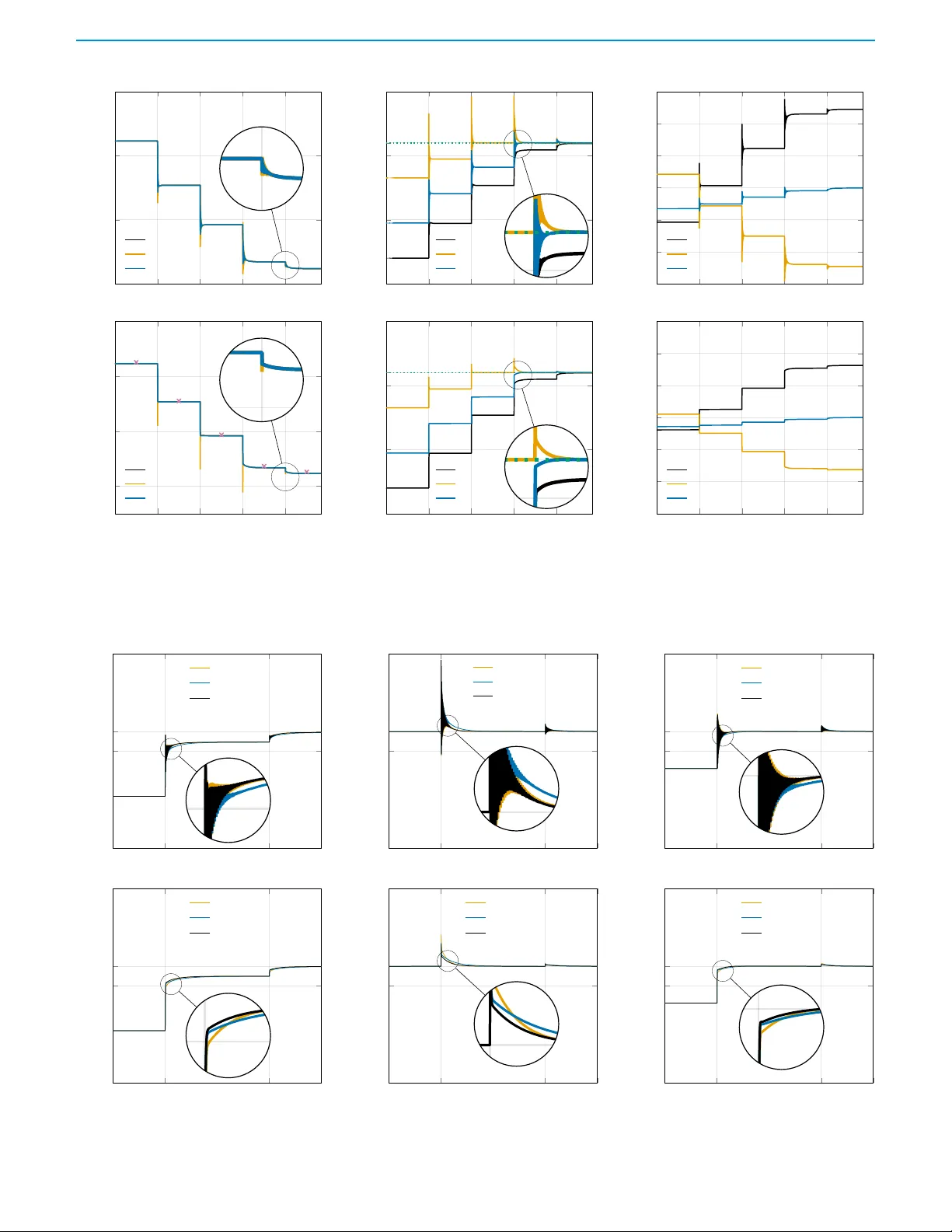
Stability and convergence of multi-converter systems using projection-free power-limiting droop control

1 Stability and con ver gence of multi-con verter systems using pr ojection-fr ee power -limiting dr oop contr ol Amirhossein Iraniparast and Dominic Groß Abstract — In this paper , we propose a projection-free power -limiting droop control for grid-connected power elec- tronics and an associated constrained flow problem. In contrast to projection-based power -limiting dr oop control, the novel pr ojection-free power -limiting droop contr ol re- sults in netw orked dynamics that are semi-globally expo- nentially stable with respect to the set of optimiz ers of the constrained flow problem. Under a change to edge coordinates, the overall networked d ynamics arising from projection-free power -limiting droop control coincide with the projection-free primal-dual dynamics associated with an augmented Lagrangian of the constrained flo w pr oblem. Leveraging this result, we (i) pro vide a bound on the con- vergence rate of the projection-free networked dynamics, (ii) pr opose a tuning method f or contr oller parameter s to impro ve the bound on the con vergence rate, and (iii) an- alyze the relationship of the bound on the con vergence rate and connectivity of the network. Finally , the analytical results are illustrated using an Electroma gnetic transient (EMT) simulation. I . I N T R O D U C T I O N The ongoing shift from synchronous machine-based power generation to wards power electronics-interfaced generation and energy storage results in significant changes to power sys- tem frequency dynamics. Specifically , grid-connected po wer electronics differ from con ventional synchronous generators in terms of their fast response (i.e., milliseconds to seconds) and resource constraints (e.g. po wer and current limits). Ac- cordingly , incorporating renewable generation resources into large-scale po wer system challenges standard operating and control paradigm and jeopardizes system stability [1], [2]. For instance, stability analysis of emerging power systems cru- cially requires considering the constraints of power con verters and renew able generation resources such as power limit. T oday , most renew ables are interfaced by dc/ac voltage source con verters (VSC) use so-called grid-following control. This control paradigm requires a stable and slowly changing ac voltage (i.e., magnitude and frequency) and jeopardizes grid stability when disturbance occur [3]. Since grid-follo wing explicitly controls the con verter current/power , incorporating power limits is straightforward. In contrast, grid-forming con- verters, that are commonly en visioned to be the cornerstone of future power systems, impose stable and self-synchronizing ac voltage dynamics at their grid terminals. Although prev alent This w ork was suppor ted in par t by the National Science Foun- dation under Grant No. 2143188. A. Iraniparast and D . Groß are with the Depar tment of Electr ical and Computer Engineering at the University of Wisconsin-Madison, USA; e-mail: iraniparast@wisc.edu, dominic.gross@wisc.edu grid-forming controls including droop control [4], virtual syn- chronous machine control (VSM) [5], and dispatchable virtual oscillator control (dV OC) [6] hav e been in vestigated in detail constraints are not accounted for in their analysis [7]–[11]. Howe ver , from a practical point of vie w , resource and con verter constraints are a significant concern. The major - ity of works on grid-forming control under constraints in the application oriented literature has focused on current- limiting (see [12] for a recent survey). Only few works in vestig ate dc voltage [13] or power limits [14]. Notably , power -limiting droop control combines conv entional droop control with proportional-integral controls that activ ate when the con verter reaches its po wer limit [14]. Continuous-time primal-dual gradient descent dynam- ics [15] have been widely used to study system-level con- trols for multi-machine systems such as automatic generation control and economic dispatch [16]. Moreover , primal-dual dynamics ha ve been used to design nov el distrib uted po wer flow controls [17]. The focus of these w orks are predominantly equality constrained optimization problems that arise from secondary and tertiary control of power systems. In contrast, this work leverages projection-free primal- dual dynamics [18] to de velop a no vel decentralized power - limiting primary control for grid-connected power electronics and analyze the resulting multi-con verter system frequency dynamics. Our novel projection-free power -limiting droop control is distinct from po wer-limiting droop control [14], [19] and enables rigorous bounds on the con vergence rate of the multi-con verter system frequency to the optimal solution of an associated constrained network flo w problem. Compared with conv entional grid-forming droop control [4], power -limiting droop control [14], [19] explicitly accounts for activ e po wer limits of resources interf aced by power con vert- ers. Moreover , the frequency dynamics of a network of VSCs using power-limiting droop control can be expressed as pro- jected dynamical system [19]. T o characterize the steady-states of these networked dynamics, a generic constrained network flow problem can be formulated whose associated primal-dual dynamics are distinct from the networked dynamics and cannot be implemented using only local information [19]. Howe ver , lev eraging a change of coordinates to edge coordinates [20], the Carath ´ eodory solutions of the projected network ed dy- namics turn out to be asymptotically stable with respect to Karush-Kuhn-T ucker (KKT) points of the constrained flow problem in edge coordinates. Specifically , in edge coordinates, the primal-dual dynamics associated with the constrained flo w problem and the projected networked dynamics coincide. This, enables to represent the networked dynamics a primal-dual 2 dynamics and apply well-known stability results [15]. Notably , the networked dynamics in nodal coordinates are globally asymptotically stable with respect to the set of optimizers of its associated constrained network problem in nodal coordi- nates [19]. This result directly establishes frequency stability and synchronization of netw orks of con verters using power - limiting grid-forming droop control. In addition, upon conv er- gence, the conv erters e xhibit po wer-sharing properties similar to so-called power -sharing in unconstrained droop control [21]. Howe ver , the discontinuity of power-limiting droop con- trol hinders con ver gence analysis and no con vergence rate is provided in [19]. In particular , while the stability of the common primal-dual gradient descent is well-studied as a discontinuous dynamical (e.g., [15]), well-known results do not provide a con vergence rate. Howe ver , from a practical point of view , bounds on the con ver gence rate are crucial for , e.g., tuning controls and analyzing performance. T o address this challenge, continuous primal-dual dynamics associated with an augmented Lagrangian hav e been introduced that are exponentially stability and admit rigorous bounds on the con ver gence rate [18], [22]. Our main contribution is to lev erage the projection-free primal-dual dynamics [22] to develop a novel projection-free power -limiting droop control, establish semi-global exponen- tial stability of the resulting networked multi-con verter fre- quency dynamics with respect to KKT points of an associated constrained flow problem, obtain a bound on the con ver gence rate of the networked multi-con verter dynamics, and analyze the impact of control gains and network parameters on the con ver gence rate. In particular , our projection-free power -limiting droop con- trol results in projection-free networked dynamics whose Carath ´ eodory solutions are semi-globally exponentially stable with respect to KKT points of the constrained flow problem introduced in [19]. T o obtain this result, we sho w that the projection-free network ed dynamics corresponds to the primal- dual dynamics of the constrained network flow problem in edge coordinates. Therefore, all existing results on the proper- ties of the KKT points of the constrained flow problem (e.g., synchronous frequency) and steady states of projection-based power -limiting droop control [19] immediately hold for the proposed projection-free power -limiting droop control. A key contribution of this work is a bound on the con- ver gence rate of the projection-free networked dynamics. T o this end, we characterize the active constraint set and graph of nodes with activ e constraints. Notably , to ev aluate the con ver gence rate of the resulting projection-free power - limiting droop control, we link the Jacobian matrix of the constraints of the network flow problem to the Laplacian matrix of the graph of nodes with activ e constraints. This result enables bounding the con ver gence rate of the networked dynamics as a function of the control gains and properties of the network (e.g., connectivity , maximum node degree, edge weights). In turn, this allows us to propose a control tuning that improv e the bound on the con ver gence rate. In addition, we show that, under mild technical assumptions, the bound on the conv ergence rate can be improv ed by adding edges (e.g., transmission lines) to the graph that increase the connecti vity of the graph. Finally , an Electromagnetic transient (EMT) simulation of the IEEE 9-bus system is used to illustrate the results and validate that the proposed control tuning improves control performance. Notation W e use R and N to denote the set of real and natural numbers and define, e.g., R ≥ 0 : = { x ∈ R | x ≥ 0 } . Moreov er , we use S n ≻ 0 and S n ⪰ 0 to denote the set of real positi ve definite and positive semidefinite matrices. For column vectors x ∈ R n and y ∈ R m we define ( x, y ) = [ x T , y T ] T ∈ R n + m . Moreov er , ∥ x ∥ = √ x T x denotes the Euclidean norm and ∥ x ∥ C : = min z ∈C ∥ z − x ∥ denotes the point to set distance. Furthermore, I n , 0 n × m , 0 n , and 1 n denote the n -dimensional identity matrix, n × m zero matrix, and column vectors of zeros and ones of length n respectiv ely . The cardinality of a discrete set X is denoted by |X | . The Kronecker product is denoted by ⊗ . W e use φ x ( t, x 0 ) to denote a (Caratheodory) solution of d d t x = f ( x ) at time t ∈ R ≥ 0 starting from x 0 at time t = 0 . I I . N E T W O R K M O D E L A N D P R E L I M I N A R I E S In this section, we introduce the ac power network model, con verter model, and conv erter control that will be considered throughout the paper . A. P ower netw ork and conv er ter model in nodal coordinates and control objectiv es Consider an ac po wer network modeled by a simple, con- nected and undirected graph G : = {N , E , W } with edge set E : = N × N corresponding to |E | = e transmission lines, set of nodes N corresponding to |N | = n voltage source con verters, and set of edge weights W = { w 1 , . . . , w e } with w i ∈ R > 0 for all i ∈ { 1 , . . . , e } modeling transmission line susceptances [23]. Throughout this work, we assume that the network is lossless, and modeled through a Kron-reduced graph. Moreov er , we model each voltage source conv erter i ∈ N as a v oltage source imposing an ac voltage with phase angle θ i ∈ R that injects an activ e power denoted by P i ∈ R . Finally , for ev ery i ∈ N , we use P L,i ∈ R to denote activ e power loads mapped from the load nodes (i.e., nodes eliminated by applying Kron reduction) to the con verter nodes. Linearizing the ac po wer flow equation at the nominal voltage magnitude and zero angle difference between nodes, results in the con verter po wer injection P : = Lθ + P L , (1) where L : = B W B T is the Laplacian matrix of the graph G , B ∈ {− 1 , 0 , 1 } n × e denotes the oriented incidence matrix of G , and W = diag { w i } e i =1 . Moreover , θ = ( θ 1 , . . . , θ n ) ∈ R n is the vector of ac voltage phase angles (relative to ω 0 t with nominal frequency ω 0 ∈ R > 0 ), P L : = ( P L, 1 , . . . , P L,n ) ∈ R n is the vector of active power loads at ev ery node, and P = ( P 1 , . . . , P n ) ∈ R n is the vector of con verter power injections. Our objectiv e is to design a (decentralized) feedback controller that maps the con verter power injection P i to the frequency 3 ω i = d d t θ i to control the power system to the solution of constrained flow problem (CFP) giv en by min θ,P 1 2 ∥ P − P ⋆ ∥ 2 M s.t. P ℓ ≤ Lθ + P L ≤ P u (2) where M : = diag { m i } n i =1 ∈ S n > 0 is a diagonal matrix of droop gains, P ⋆ : = ( P ⋆ 1 , . . . , P ⋆ n ) ∈ R n is a vector of local references, and P ℓ : = ( P ℓ, 1 , . . . , P ℓ,n ) ∈ R n and P u : = ( P u, 1 , . . . P u,n ) ∈ R n model limits on the network injections. The following assumptions ensure feasibility of (3). Assumption 1 ( Feasible injection limits and loads ) F or all i ∈ N , the limits P ℓ,i ∈ R n and P u,i ∈ R n satisfy P ℓ,i < P u,i . Mor eover , the disturbance input P L ∈ R n satisfies P n i =1 P ℓ,i < P n i =1 P L,i < P n i =1 P u,i . Assumption 2 ( Feasible references ) The setpoints P ⋆ i ∈ R n satisfy P ℓ,i < P ⋆ i < P u,i . The ne xt proposition ensures feasibility of the CFP (3) under Assumption 1. Proposition 1 ( Feasibility in nodal coordinates [19] ) There exists θ ∈ R n such that P ℓ < Lθ + P L < P u if and only if P ℓ , P u , and P L satisfy Assumption 1. Finally , we define S θ as the set of KKT points of (1) (for de- tails see [19, Def. 1]). Moreover , let K I : = diag { p k I ,i } n i =1 ∈ S n > 0 denote a diagonal matrix scaling the constraints. The set of KKT points of min θ 1 2 ∥ Lθ ∥ 2 M + ( P L − P ⋆ ) T M Lθ (3a) s.t. K I P ℓ ≤ K I ( Lθ + P L ) ≤ K I P u (3b) is identical to S θ [19]. B. P ower networ k and conv er ter model in edge coordinates Using the oriented incidence matrix B and V : = W 1 2 ∈ R n × n , we define the change of coordinates η = V B T θ as the so-called edge coordinates [20]. The power injection (1) in edge coordinates follows P : = B V η + P L . (4) Next, consider the constrained flow problem in edge coordi- nates min η 1 2 ∥ B V η ∥ 2 M + ( P L − P ⋆ ) T M B V η (5a) s.t. K I P ℓ ≤ K I ( B V η + P L ) ≤ K I P u . (5b) Assumption 3 The linear independence constraint qualifica- tion (LICQ) holds at any optimizer η ⋆ of (5) . Finally , we define S η as the set of KKT points of (4) (for details see [19, Def. 8]). C . Graph of nodes with active constraints Using the following definitions, we introduce the acti ve constraint graph associated with G . w 2 w 1 w 3 w 6 w 7 w 4 w 5 w 2 w 1 w 3 w 4 w 5 Fig. 1 : The graph G and the activ e graph G I corresponding to L I : inactiv e constraint nodes (blue), activ e constraint nodes (red), edges connecting activ e constraint nodes (orange), and edges connecting active and inactive constraint nodes (green). Definition 1 ( Active constraint sets ) W e define I ℓ ⊆ N and I u ⊆ N \ I ℓ as the set of nodes at their lower and upper limit, i.e., i ∈ I ℓ if and only if P i = P ℓ,i and i ∈ I u if and only if P i = P u,i . Mor eover , we define I : = I ℓ ∪ I u . Definition 2 ( Graph of nodes with active constraint ) Let B I contain the r ows of B associated with the active set I . Mor eover , we define the graph G I containing nodes i ∈ I and edges ( i, j ) ∈ ( I × I ) ∩ E . Additionally , edges connecting nodes i ∈ I and nodes j / ∈ I appear as self-loops in G I . By extracting the weights corresponding to active nodes as W I , we define the Laplacian matrix associated with G I as L I = B I W I B T I , where removing the rows of B corre- sponding to inactiv e nodes results in B I with (i) fully zero columns associated with edges of the inacti ve part of the graph, (ii) columns containing only 1 or − 1 associated with edges connecting the inactiv e part of the graph to that of the active part and (iii) columns containing 1 and − 1 associated with edges of the active part of the graph. It should be noted that the edges connecting the inacti ve to the acti ve part of the graph represent themselves as self-loops in L I (see Fig. 1). Now we can discuss the relation between the Laplacian L I and the Jacobian of the of CFP constraints in edge coordinates. Let J denote the Jacobian of the constraints (5b). At any optimizer η ⋆ of (5), we define κ : = λ min  J I ℓ ∪I u J T I ℓ ∪I u  , where J I contains the row vectors of the Jacobian J whose indices are in I . Moreov er , Assumption 3 implies that κ > 0 . As shown in the next proposition κ is equi v alent to the minimum eigen value of the Laplacian L I scaled with the controller gains K I I of the inactiv e nodes. Proposition 2 F or any diagonal matrix K I I ∈ S n ≻ 0 and Laplacian L I , it holds that κ = λ min ( K I I L I K I I ) . Pr oof. Suppose that I ℓ ∪ I u = I , since we ha ve J I = ( K I B V ) I = K I I B I V I , then by the definition of κ , and Definition 2, it immediately follows that κ = λ min ( K I I B I V I V I B T I K I I ) and κ = λ min ( K I I L I K I I ) . It follows from [19, Proposition 2] that either I ℓ = ∅ or I u = ∅ . This immediately results in the following corollary . 4 Dro op con trol P ow er-limiting (pro jection) m i + + P i − + P ⋆ i ω i − + P u,i k I ,i k P,i − + − R 0 ∞ + + − P ℓ,i k I ,i k P,i + + R 0 ∞ Fig. 2 : Projection-based power -limiting droop control Corollary 1 It holds that either κ = λ min  J I ℓ J T I ℓ  or κ = λ min  J I u J T I u  . Mor eover , for uniform contr oller gains, i.e., k I ,i = c ∈ R > 0 for all i ∈ N , it holds that κ = cλ min ( L I ) . I I I . P R O J E C T I O N - F R E E P OW E R L I M I T I N G D R O O P C O N T R O L In this section, we first revie w results for (projection-based) power -limiting droop control [14], [19]. Then we introduce the nov el projection-free power -limiting droop control. A. Revie w of projection-based network dynamics Computing the optimal solution of (3) via its associated primal-dual dynamics [15] results in a distributed algorithm that requires exchanging dual-multipliers between nodes. This is not feasible on primary frequency control timescales in large-scale power systems. In contrast, the projection-based network dynamics depicted in Fig. 2, that resemble but are distinct from the well-kno wn primal-dual dynamics, solve (3) using only local information [19]. W e require the following definition of projection operator to formalize the projection- based and projection-free network dynamics. Definition 3 ( Projection ) Given a conve x set C ⊆ R n and a vector v ∈ R n , Π C ( v ) denotes the pr ojection of v with r espect to the set C , i.e., Π C ( v ) = argmin p ∈C ∥ p − v ∥ . Next, consider the projection-based power -limiting droop control with states d d t θ i = ω i , λ u,i ∈ R ≥ 0 , and λ ℓ,i ∈ R ≥ 0 that correspond to the ac v oltage phase angles and integral of the upper and lower po wer limit violations (see Fig. 2). Let g ( P N ) =  g ℓ ( P N ) g u ( P N )  : =  P ℓ − P N − P L P N + P L − P u  . The interconnection of the nodal dynamics in Fig. 2 via (1) can be written as the projected dynamical system d d t θ = M ( P ⋆ − P L − Lθ ) − (Ξ ⊗ K I ) λ (6a) − (Ξ ⊗ K P ) Π R 2 n ≥ 0 ( g ( Lθ )) , d d t λ =Π T λ R 2 n ≥ 0  ( I 2 ⊗ K I ) g ( Lθ )  , (6b) Dro op con trol P ow er-limiting (pro jection-free) m i + + P i − + P ⋆ i ω i − + P u,i ρ − + + − + k I ,i R 1 ρ + − P ℓ,i ρ + + − k I ,i R 1 ρ Fig. 3 : Projection-free power -limiting droop control where Ξ : = ( − 1 , 1) T and λ : = ( λ ℓ , λ u ) ∈ R 2 n ≥ 0 collects the integrator states. Moreov er , the matrix K P : = diag { k P,i } n i =1 collects proportional gains k P,i ∈ R > 0 . W e emphasize that this model assumes that the load P L , power setpoints P ⋆ , and power limits P ℓ and P u are constant on the time-scales of interest for studying frequency stability . While multi-con verter network dynamics (6) do not coincide with the primal-dual dynamics of (3) in nodal coordinates, they coincide after transformation to edge coordinates. Notably , using η = V B T θ to transform the multi-conv erter network dynamics (6) results in dynamics that coincide with the primal- dual dynamics of the CFP (5) in edge coordinates (see [19, Fig. 1]). Building upon this observation and the LaSalle function from [15], it can be shown that (6) con ver ges to optimal (i.e., KKT) points of (3) [19]. Ho we ver , this analysis does not provide a con vergence rate. In addition, due to the discontinuity of the dual dynamics, the projection-based network dynamics (6) cannot con ver ge exponentially [22]. In the next section, we introduce the projection-free net- worked dynamics that are the main focus of this paper . B. Projection-free networked dynamics T o overcome these conceptual limitations of projection- based power -limiting droop control, we introduce the nov el projection-free power -limiting droop control (see Fig. 3) d d t θ i = m i ( P ⋆ i − P i ) − k I ,i Π R ≥ 0 ( ρ ( P i − P u,i ) + λ u,i ) (7a) + k I ,i Π R ≥ 0 ( ρ ( P ℓ,i − P i ) + λ ℓ,i ) , d d t λ ℓ,i = 1 ρ  Π R ≥ 0 ( ρ ( P ℓ,i − P i ) + λ ℓ,i ) − λ ℓ,i  , (7b) d d t λ u,i = 1 ρ  Π R ≥ 0 ( ρ ( P i − P u,i ) + λ u,i ) − λ u,i  . (7c) This controller is moti vated by the projection-free primal- dual dynamics introduced in [18], [22]. The reminder of this manuscript analyzes the interconnection of the nodal dynamics (7) via (1) giv en by d d t θ = M ( P ⋆ − Lθ − P L ) − (Ξ ⊗ K I )Π R 2 n ≥ 0 ( ρg ( Lθ ) + λ ) , (8a) ρ d d t λ = Π R 2 n ≥ 0 ( ρg ( Lθ ) + λ ) − λ. (8b) 5 W e emphasize that the projection-free multi-con verter fre- quency dynamics (8) do not coincide with the projection- free primal-dual dynamics associated with the CFP (3) in nodal coordinates. Howe ver , applying the change of coordi- nates to edge coordinates, the projection-free multi-conv erter frequency dynamics coincide with the projection-free primal- dual dynamics of (5). Thus, [22, Theorem 1] can be used to establish exponentially con ver gence of the multi-con verter frequency dynamics to KKT points of (3) and bound the con ver gence rate. I V . S T A B I L I T Y O F P R O J E C T I O N - F R E E N E T W O R K E D DY N A M I C S I N E D G E C O O R D I N A T E The Augmented Lagrangian introduced in [24] associated with the CFP in edge coordinates (5) is given by L ( η , µ ℓ , µ u ) = 1 2 ∥ B V η ∥ 2 M + ( P L − P ⋆ ) T M B V η + m X j =1 H ρ ( − a T j η − b j , µ j,ℓ ) + H ρ ( a T j η − c j , µ j,u ) (9) with penalty function H ρ ( a T j η − b j , µ j ) = ( ( a T j η − b j ) µ j + ρ 2 ( a T j η − b j ) 2 if ρ ( a T j η − b j ) + µ j ≥ 0 − 1 2 µ 2 j ρ if ρ ( a T j η − b j ) + µ j < 0 Here, a j is the j -th column of ( K I B V ) T , b j is the j -th element of K I ( P L − P ℓ ) , c j is the j -th element of K I ( P u − P L ) , and µ ℓ ∈ R ≥ 0 and µ u ∈ R ≥ 0 are the dual multipliers associated with the lower and upper inequalities respectiv ely . Note that P n j =1 x j Π R ≥ 0 ( y j ) = X T Π R n ≥ 0 ( y ) , where x j is the j -th column of matrix X and y j is the j -th element of the column vector y . Then, primal-dual gradient dynamics associated with (9) are giv en by µ = ( µ ℓ , µ u ) and d d t η = V B T  M ( P ⋆ − P L − B V η ) (11a) − (Ξ ⊗ K I )Π R 2 n ≥ 0  ρ ( I 2 ⊗ K I ) g ( B V η ) + µ   ρ d d t µ =Π R 2 n ≥ 0  ρ ( I 2 ⊗ K I ) g ( B V η ) + µ  − µ. (11b) The next theorem establishes the projection-free network ed dynamics (8) and projection-free primal-dual dynamics (11) coincide in edge coordinates. T o this end, let T η : = blkdiag( V B T , K I ) . Theorem 1 ( Coinciding dynamics ) Consider any initial con- dition ( θ 0 , λ 0 ) of the pr ojection-free networked dynamics (8) in nodal coor dinates. Mor eover , consider the corr esponding initial condition ( η 0 , µ 0 ) = T η ( θ 0 , λ 0 ) of the pr ojection-fr ee primal-dual dynamics (11) of (9) in edge coordinates. Then, the solutions φ θ ( t, ( θ 0 , λ 0 )) and φ η ( t, ( η 0 , µ 0 )) of (8) and (11) satisfy T η φ θ ( t, ( θ 0 , λ 0 )) = φ η ( t, T η ( θ 0 , λ 0 )) . Pr oof. Using the change of v ariables µ = K I λ and [19, Lemma 2], the networked dynamics (8) can be written as d d t θ = M ( P ⋆ − Lθ − P L ) (12a) − (Ξ ⊗ K I )Π R 2 n ≥ 0 ( ρ ( I 2 ⊗ K I ) g ( Lθ ) + µ ) ρ d d t µ =Π R 2 n ≥ 0  ρ ( I 2 ⊗ K I ) g ( Lθ ) + µ  − µ (12b) Recalling the definition g ( P N ) and using edge coordinate η = V B T θ , the network dynamics in edge coordinates become identical to (11). Moreover , since d d t η ∈ Im V B T holds for (11a) and any initial condition η 0 ∈ Im V B T , it holds that η ∈ Im V B T for all t ∈ R ≥ 0 . For any initial condition ( θ 0 , µ 0 ) trajectories of (12) mapped to the edge coordinates coincide with trajectories of (11) with the initial condition ( V B T θ 0 , µ 0 ) . W e conclude that the projection-free networked dynamics (7) mapped to edge coordinate coincide with the primal-dual dynamics associated with (9) for any initial condition η 0 ∈ Im( V B T ) . Before establishing stability of the network dynamics in edge coordinate (11), we need to extend the definition of semi- global exponential stability [25, Theorem 5.17] to semi-global exponential stability with respect to a set. Definition 4 ( Semi-global exponential stability ) Consider the autonomous dynamical system d d t z ( t ) = ϕ ( z ( t )) and its set Z e of equilibrium points. Any point z e ∈ Z e is a semi- global exponentially equilibrium point, if for any h > 0 , there exist M β > 0 and β > 0 such that for any initial point z 0 such that ∥ z 0 ∥ Z e ≤ h , the corresponding solution z ( t ) of the dynamical system satisfies ∥ z ( t ) ∥ Z e ≤ M β · e − β t ∥ z (0) ∥ Z e , ∀ t ∈ [0 , ∞ ] . Although Definition 4 does not require any properties on the set of equilibrium points, in our analysis Z e is a con ve x set of points satisfying KKT conditions. The next proposition states bounds for the maximum eigen- value of Laplacian L . Proposition 3 Consider the de gr ee d i of node i ∈ N , the minimum and maximum edge weights w min and w max , and maximum node degr ee d max : = max i ∈N d i . Then, the lar gest eigen value of the Laplacian L is bounded by w min (1 + d max ) ≤ λ max ( L ) ≤ 2 w max d max . (13) A proof is provided in the Appendix. W e are no w ready to state our main stability result. Theorem 2 ( Semi-global exponential stability of primal– dual dynamics in edge coordinates ) Consider P ℓ , P u , P L , and P ⋆ such that Assumption 1 and Assumption 2 hold. Then, under Assumption 3, the primal-dual dynamics (11) ar e semi- globally exponentially stable with respect to S η on R e × R 2 n ≥ 0 . Mor eover , d d t ( η , λ ) = 0 e +2 n holds on S η . A proof is provided in the Appendix. W e emphasize that the frequency and activ e constraints upon con ver gence for both projection-based and projection- free po wer limiting droop control are identical and solely de- termined by the KKT points of (3). In particular, synchronous frequency ω s can be explicitly expressed as a function of the activ e sets I u and I ℓ , total load P i ∈N P L,i , total power dispatch P i ∈N P ⋆ i , and droop coefficients [19, Th. 3]. V . C O N V E R G E N C E R A T E In this section, before addressing the con ver gence rate, we study the stability of the proposed networked dynamics in nodal coordinates. 6 A. Preliminar ies Proposition 4 ( Semi-global exponential stability of net- worked dynamics in nodal coordinates ) Consider P ℓ , P u , P L , and P ⋆ such that Assumption 1 and Assumption 2 hold. F or any connected graph G , (8) is semi-globally exponentially stable on R n × R 2 n ≥ 0 with r espect to the set S θ . Mor eover , there exists ω s ∈ R such that lim t →∞ ω i ( t ) = ω s for all i ∈ N . Pr oof. Definition 4 does not restrict the initial condition and we consider nonneg ativ e initial v alues λ (0) , µ (0) ≥ 0 . In this case, the dual multipliers remain in nonnegati ve orthant [22, Proposition 1]. Next, we can establish the stability of the dynamical system in original coordinates. Notably , there exist κ ∈ R ≥ 0 and κ ∈ R ≥ 0 , ∀ t ≥ 0 such that κ ∥ T η φ θ ( t, ξ 0 ) ∥ S η ≤ ∥ φ θ ( t, ξ 0 ) ∥ S θ ≤ κ ∥ T η φ θ ( t, ξ 0 ) ∥ S η (14) By [19, Theorem 1], it follo ws that the left inequality holds with κ = ∥ T η ∥ − 1 . Next, let σ 1 : = min θ ⊥ 1 n , ∥ θ ∥ =1   V B T θ   ∈ R > 0 . Then, the upper bound of (14) holds with κ = 1 min { 1 ,σ 1 } . By Theorem 2, (11) is semi-globally exponentially stable on R e × R 2 n ≥ 0 with respect to S η . Using Theorem 2 and the upper bound of (14), we hav e ∥ φ η ( t, T η ξ 0 ) ∥ S η ≤ M β · e − β t ∥ φ η (0 , T η ξ 0 ) ∥ S η where ∥ φ θ ( t, ξ 0 ) ∥ S θ ≤ κ ∥ φ η ( t, T η ξ 0 ) ∥ S η and M β is a constant depending on the decaying rate β . Moreov er , we have ∥ φ η (0 , T η ξ 0 ) ∥ S η ≤ κ − 1 ∥ φ θ (0 , ξ 0 ) ∥ S θ . Finally , we conclude ∥ φ θ ( t, ξ 0 ) ∥ S θ ≤ κ · κ − 1 · M β · e − β t ∥ φ θ (0 , ξ 0 ) ∥ S θ . In other words, (7) is semi-globally exponentially stable on R n × R 2 n ≥ 0 with respect to the set S θ . In addition, we show that lim t →∞ ω ( t ) = 1 n ω s . According to Theorem 2, any pair ( η ⋆ , λ ⋆ ) con ver ges to a KKT point ( η ⋆ , λ ⋆ ) ∈ S η , i.e., lim t →∞ η ( t ) = η ⋆ and lim t →∞ d d t η = 0 e . Using η = V B T θ , we obtain lim t →∞ d d t V B T θ ( t ) = lim t →∞ V B T d d t θ ( t ) = lim t →∞ V B T ω ( t ) = 0 and lim t →∞ ω ( t ) = 1 n ω s follows ker( B T ) = span( 1 n ) to conclude the proof. B. Conv ergence rate Next, using results for the primal-dual gradient dynamics associated with the augmented Lagrangian [15], [22], globally asymptotic stability of the projection-free networked dynamics in nodal coordinate (7) can be established. Ho wev er , since the gradient of the constraints (5b), i.e., B V is not full row rank, a global exponential con ver gence rate cannot be obtained [26]. W e begin by introducing se veral constants that are needed to establish semi-global exponential conv ergence of the projection-free networked dynamics. First, let M g denote an upper bound on the spectral norms of the Jacobian J giv en by the maximum control gain k I , max : = max i ∈N k I ,i , M g = p 2 k I , max w max d max (see Prop. 3), and ∥ K I B V ∥ 2 ≤ ∥ K I ∥ 2 ∥ B V ∥ 2 ≤ q k I , max λ max ( L e ) (15a) ≤ q k I , max λ max ( L ) ≤ M g . (15b) Next, let L g denote an upper bounds on the Frobenius norms of the Jacobian J of the constraint (5b) giv en by ∥ K I B V ∥ F ≤ ∥ K I ∥ 2 ∥ B ∥ 2 ∥ V ∥ F (16a) ≤ p 2 d max k I , max w Σ = L g (16b) where we used w Σ : = P e j =1 w j , ∥ B ∥ 2 = p ∥ B ∥ 1 ∥ B ∥ ∞ , ∥ B ∥ ∞ = d max , and ∥ B ∥ 1 = 2 . Using M g and L g , we define M θ ( ρ, L g , M g ) = ρL 2 g + M g ( ρL g d 0 + d 0 + ∥ µ ⋆ ∥ ) . (17) Moreov er , we define the edge Laplacian associated with the Laplacian L as L e = V B T B V , then we hav e m min λ max ( L e ) ≤ λ max ( V B T M B V ) ≤ m max λ max ( L e ) . Using λ max ( L e ) = λ max ( L ) [20] and Proposition 3, γ = λ max ( V B T M B V ) , we hav e m min w min (1 + d max ) ≤ γ ≤ 2 m max w max d max . Finally , we require α -strong con ve xity of (5a) and γ - lipschitzness of its gradient. T o this end, note that λ min (Γ T + V B T M B V Γ + ) = λ + min ( V B T M B V ) In addition, m min λ + min ( L ) ≤ λ + min ( V B T M B V ) where λ + min ( L ) is the algebraic connectivity of the graph G . Thus, we conclude that 1 0 < α ≤ α ≤ γ ≤ γ with α = m min λ + min ( L ) and γ = 2 w max m max d max . Next, recall the conditions on the con vergence rate β [22] β ≤ κδ min 46 ρL 2 g , (22a) κα 4 β − 4 β 2 ≥ L 2 g + κ 4 + ( γ + M θ )( α + M θ + 1 ρ ) + 1 2 ρ 2 . (22b) Moreov er , we define δ min ( ρ, k I ,i ) : = 1 −  1 + ρ · max i ∈ N \ ( I u ∪I ℓ ) p k I ,i g i ( η ⋆ ) d 0  2 + , where d 0 ∈ R > 0 is the point to set distance of initial primal- dual pair ( η 0 , µ ℓ, 0 , µ u, 0 ) to the set of KKT points S η . W e can now state the following corollary that establishes semi-global exponential con ver gence of the projection-free networked dynamics. Corollary 2 Let β ∈ R > 0 denote any strictly positive constant satisfying (22) . Then, ther e exists M β ∈ R > 0 such that lim β → 0 + M β = 1 and ∥ φ θ ( t, ξ 0 ) ∥ S θ ≤ κ · κ − 1 · M β · e − β t ∥ φ θ (0 , ξ 0 ) ∥ S θ . The corollary directly follows from [22, Theorem 1]. 1 This bound holds for any graph G with n ≥ 3 . Moreover , for n = 2 the second-smallest eigen value can be obtained explicitly . 7 C . Control tuning Although the bounds in Corollary 2 explicitly depend on ρ , changing the controller gains implicitly manipulate the boundaries by changing the other parameters. Accordingly , it is crucial to address how to choose the controller gains to improv e the closed-loop con ver gence rate. T o this end, the next proposition introduces the idea to manipulate the given gain ρ and controller gains k i to enlarge the boundaries. Proposition 5 Consider contr oller gains k I ,i ∈ R > 0 and ρ ∈ R > 0 . Moreo ver , let k ′ i = sk I ,i and ρ ′ = 1 √ s ρ . F or all s ∈ R > 1 , it holds that β ( k I ,i , ρ ) < β ( k ′ i , ρ ′ ) . Pr oof. Let ζ β = α β − 16 β 2 κ , ζ 1 = 4 L 2 g κ , and ζ 2 = 4 κ  ( γ + M θ )( α + M θ + 1 ρ ) + 1 2 ρ 2  . Under the conditions of Corollary 2, it holds that ζ β ≥ ζ 1 + ζ 2 + 1 . Notably , ζ β is an increasing function with respect to κ , i.e., ∂ ζ β ∂ κ = 16 β 2 κ 2 > 0 . Scaling the gains k ′ I ,i = sk I ,i , we obtain L ′ g = √ s k L g , κ ′ = sκ and M ′ g = √ sM g respectiv ely . In other words, ζ β increases and ∂ ζ 1 ∂ s = ∂ ∂ s 4 L ′ g 2 κ ′ 2 = 0 . Therefore, it is sufficient to show that ζ 2 decreases under scaling by s . Expanding ζ 2 results in ζ 2 = 4  γ α κ + ( γ + α ) M θ κ + γ κρ + M θ ( M θ + 1 ρ ) κ + 1 2 κρ 2  . Note that ∂ ∂ s γ α κ ′ < 0 and ∂ ∂ s γ κ ′ ρ ′ < 0 , i.e., the first and third term decrease as s increases. Moreover , the last term is unchanged since ∂ ∂ s 1 κ ′ ρ ′ 2 = 0 . Ne xt, we show that the second term of ζ 2 decreases and the fourth term of ζ 2 is unchanged as s increases. For brevity consider M ′ θ = M θ ( ρ ′ , L ′ g , M ′ g ) resulting in ∂ ∂ s M ′ θ κ ′ = ∂ ∂ s ρ ( L 2 g + L g M g d 0 ) √ sκ + ∂ ∂ s M g ( d 0 + ∥ µ ⋆ ∥ ) √ sκ < 0 . Additionally , for the fourth term ∂ ∂ s M ′ θ 2 κ ′ = ∂ ∂ s ρ 2 ( L 2 g + M g L g d 0 ) 2 κ + ∂ ∂ s M 2 g ( d 0 + ∥ µ ⋆ ∥ ) 2 κ + ∂ ∂ s 2 ρ ( L 2 g + M g L g d 0 ) M g ( d 0 + ∥ µ ⋆ ∥ ) κ = 0 and ∂ ∂ s M ′ θ κ ′ ρ ′ = ∂ ∂ s ρL 2 g + M g ( ρL g d 0 + d 0 + ∥ µ ⋆ ∥ ) κρ = ∂ ∂ s L 2 g κ + ∂ ∂ s M g L g d 0 κ + ∂ ∂ s M g ( d 0 + ∥ µ ⋆ ∥ ) κρ = 0 . W e conclude that κα 4 β − 4 β 2 increases for any increasing s > 1 , i.e., ∂ ζ 2 ∂ s < 0 . Moreover , recalling β ≤ κδ min 46 ρL 2 g and the definition of δ min we hav e δ min ( ρ, k I ,i ) : = 1 −  1 + ρ · max i ∈ N \ ( I u ∪I ℓ ) p k I ,i g i ( η ⋆ ) d 0  2 + . This implies that ∂ ∂ s κ ′ δ min ( ρ ′ ,k ′ I ,i ) 46 ρ ′ L ′ g 2 = ∂ ∂ s √ sκδ min ( ρ,k I ,i ) 46 ρL 2 g > 0 . Due to enlargement of both bounds on β in Corollary 2, irrespectiv e of the dependency of M β on β , we conclude that β ( k I ,i , ρ ) < β ( k ′ i , ρ ′ ) . This result establishes that the conv ergence rate increases for increasing s ∈ R > 1 , i.e., increasing k I ,i and decreasing ρ according to Proposition 5. Next, we bound the maximum achiev able conv ergence rate. Proposition 6 The maximum con ver gence rate β max is bounded by min { κδ min 46 ρL 2 g , ˜ c } ≤ β max ≤ 1 46 ρ , wher e ˜ c = 3 r − q 2 + q q 2 4 + p 3 27 + 3 r − q 2 − q q 2 4 + p 3 27 , c = 5 4 L 2 g + ( γ + M θ )( γ + M θ + 1 ρ ) + 1 2 ρ 2 , p = c 4 , and q = − κα 16 . Pr oof. By the definition of κ , it holds that κ < L 2 g . Since δ min ≤ 1 , this results in the upper bound. Solving (22b) resulting from the second inequality in Corollary 2 results in the lower bound. This result establishes that the upper bound on the maximum achiev able conv ergence rate β max increases as the gain ρ de- creases. On the other hand, the lower bound on the maximum achiev able con ver gence rate β max has a non-tri vial dependence on both the controller gains and network topology . Finally , we bound the gains ρ to narrows down the range of gains ρ to be considered for controller tuning. Proposition 7 The gain ρ ⋆ corr esponding to the maximum con ver gence rate β in Cor ollary 2 is bounded by 2 c 1 23 κα < ρ ⋆ ≤ 1 + 1 23 κα max { 2 c 1 , 2 γ , 1062 1058 } . Pr oof. Since κα 4 β − 4 β 2 is a decreasing function of β , any ρ that satisfy the conditions of Corollary 2 satisfies 23 2 καρ 3 − c 1 ρ 2 − γ ρ − 531 1058 > 0 where c 1 = L 2 g + κ 4 + γ α . Therefore, since γ ρ + 531 1058 > 0 we hav e 23 2 καρ 3 > c 1 ρ 2 and ρ > 2 c 1 23 κα . Moreover , an upper bound on the solution is giv en by ρ ≤ 1 + 1 23 κα max { 2 c 1 , 2 γ , 1062 1058 } The result follows from feasibility of the optimum ρ ⋆ . D . Impact of networ k topology In addition to the control gains, the con vergence rate of the projection-free networked dynamics crucially depends on the network topology and edge weights (e.g., transmission line susceptances). In this section, we analyze the impact of key network parameters on the con ver gence rate. T o this end, recall that d i , i ∈ N , and d max denotes the node degree and maximum node degree. The follo wing proposition 8 r 1 r 2 r 3 f 2 β f ( α, β ) r 1 r 3 r 2 f 2 β f ( α, β ) r 3 r 1 r 2 f 2 β f ( α, β ) Fig. 4 : Representative different cases of bounds (22a) and (22b) indicating the decaying rate β , f ( α, β ) and f 2 are left and righthand side of the bound (22b) respectiv ely , where r 1 = arg β ( f ( α, β ) = f 2 ) , r 2 = 3 p κα 16 , and r 3 = κδ min 46 ρL 2 g . establishes that, under some technical assumptions, the con- ver gence rate β increases when the connecti vity of the graph G increases. Proposition 8 Consider adding an edge with weight w e +1 ≤ w max between any two nodes ( i, j ) / ∈ E that satisfy d l < d max , l ∈ i, j . Then, β ( ρ, k I ,i ) remains unchanged if (22a) is binding. On the other hand, β ( ρ, k I ,i ) increases if (22b) is binding and ρ ∈ R > 0 satisifies ( 21 2 − cd 0 ) ρ ≥ m max k i, max c 2 + d 0 + ∥ µ ⋆ ∥ p 2 k i, max d max w Σ c with c = q w max w Σ . Pr oof. Adding the edge ( i, j ) between these nodes increases the connectivity λ + min ( L ) . In turn, this results in increased α . Let f ( α, β ) : = κα 4 β − 4 β 2 , and f 2 = L 2 g + κ 4 + ( γ + M θ )( α + M θ + 1 ρ ) + 1 2 ρ 2 . Then, (22b) can be written as f ( α, β ) ≥ f 2 . Moreover , f ( α , β ) ≥ f 2 is satisfied for all β ≤ min { κδ min 46 L 2 g , arg β ( f ( α, β ) = f 2 ) } . T aking the deriv ativ e of f ( α , β ) ≥ f 2 with respect to α and rearranging the resulting inequality results in β ≤ κ 4( γ + M θ ) . Thus, if (22a) is binding, then β ( ρ, k I ,i ) is unchanged. Other - wise, (22b) is binding if κ 4( γ + M θ ) ≤ κδ min 46 L 2 g . This results in 46 ρL 2 g ≥ δ min 4( γ + M θ ) . Since δ min ≤ 1 it is sufficient to sho w 46 ρL 2 g ≥ 4( γ + ρL 2 g + M g ( ρL g d 0 + d 0 + ∥ µ ⋆ ∥ )) . For this inequality to hold, ρ has to satisfy (1 − 2 21 M g L g d 0 ) ρ ≥ 2 21 γ L 2 g + 2 21 M g L 2 g ( d 0 + ∥ µ ⋆ ∥ ) . In addition, γ L 2 g ≤ m max w max k I , max w Σ , M g L 2 g = √ w max √ k I , max d max w Σ , and M g L g d 0 = q w max w Σ d 0 . This results shows that, under mild technical assumptions, adding edges that connect previously weakly connected nodes (i.e., increasing the connecitivity of the network) increases the con ver gence rate of the projection-free networked dynamics. Specifically , on a suf ficiently large gain ρ , the con vergence rate can be improved by introducing an edge with a weight equal or lower than w max connecting any two nodes with degree less than d max . Moreov er , the following corollary establishes the same result for the simpler setup of a graph with identical weights. Corollary 3 Consider a graph G with uniform edge weights w i = w ′ for all i ∈ { 1 , . . . , e } and let k i, max = s m m max denote the contr oller gain as function of the maximum dr oop gain m max and s m ∈ R > 1 . F or any connected graph G with n ≥ 3 the lower bound on ρ in Pr oposition 8 can be replaced by (21 e − 2 √ ed 0 ) ρ ≥ 2 s m + d 0 + ∥ µ ⋆ ∥ p k i, max w ′ (23) wher e e is the number of edges. Corollary 3 shows that, as long as the number of edges e and distance d 0 of the initial primal-dual pair satisfy 21 e − 2 √ ed 0 > 0 , increasing the number of edges e improves the bound on ρ for which Prop. 8 holds. In other words, adding edges as outlined in Prop. 8 improv es the con vergence rate for lower gains ρ if the initial number of edges e is larger . V I . N U M E R I C A L C A S E S T U DY T o illustrate and validate our analytical results obtained for the reduced-order model (7) and (1) of the frequenc y dynamics of multi-con verter po wer systems, we use an electromagnetic transient (EMT) simulation of the IEEE 9-bus system (see Fig. 5) with three VSCs controlled by power limiting droop control. A. P ower system model Specifically , we replaced the three synchronous generators in the IEEE 9-bus system with voltage source con verters (VSCs). An average model of two-lev el VSCs with LC output filter and standard cascaded inner voltage and current loops is used. Details on the transformer parameters, con verter parameters, and control gains of the inner control loops can be found in [27]. T able I and [19, T able I] summarize the con verter rating, power setpoints, power limits, and control gains for power -limiting droop control used in this work. In addition to the standard IEEE 9-bus base load a time- varying constant power load (see Fig.5) is introduced to create ov erload conditions for the VSCs. Notably , the reduced-order model (7) is obtained by applying kron-reduced [23] to obtain a network model with three buses and assuming that activ e power and frequency are decoupled from reactiv e power and voltage magnitude. 9 1 4 9 5 6 3 8 7 2 45 MW 45 MW 45 MW P d ( t ) VSC 1 S c = 100MV A 1kV 13.8kV S T =100MV A 13.8kV 230kV S T =210MV A VSC 2 S c =100MV A 230kV 13.8kV S T =210MV A 13.8kV 1kV S T =100MV A VSC 3 S c =100MV A 1kV 13.8kV S T =100MV A 13.8kV 230kV S T =210MV A S b =100MV A, ω b = 2 π 50 5 35 65 95 125 150 0 0 . 65 1 . 28 1 . 75 1.80 t [s] P d [pu] A ctive p ow er load Fig. 5 : IEEE 9-bus test case system with three two-le vel voltage source conv erters and constant impedance (black) and constant power loads (red). B. Simulation results and discussion Simulation results are shown in Fig. 6 and Fig. 7. EMT simulation results are shown in the top row and simulation results obtained using the reduced-order model (7) are shown in the bottom row . The pink markers in the bottom row of Fig. 6 indicate the frequency deviation predicted by [19, Theorem 3]. Under the same load profile used in [19], we validate the analytical results for the synchronous frequency , and observe that the analytical results closely match the EMT simulation and results obtained using the reduced-order model (7). Finally , to compare projection-based [19] and projection- free power -limiting droop control (7) the response of active power to a load increase and subsequent conv ergence are shown in Fig. 7. Notably , before the load increase at t = 95 s , VSC 2 is overloaded. In addition, the load increase at t = 95 s ov erloads VSC 3. Moreover , after the load increase at t = 125 s all VSCs operate at their maximum activ e power . In addition, we validate the improvement of the con ver gence rate according to Proposition 5 by scaling controller gains, i.e., using the scaling s = 1 . 66 improves the con vergence rate relativ e to using the scaling s = 1 . T ABLE I : Model and control parameters. For further details see [27, T able I]. VSC Power [MW] Control gains [pu] P ⋆ P ℓ P u m p ρ k I 1 25 MW 20 MW 110 MW 4.17% 1.02 40.95 2 87.5 MW 20 MW 110 MW 9.38% 1.02 40.95 3 55 MW 20 MW 110 MW 6% 1.02 40.95 V I I . A P P E N D I X Pr oof of Pr oposition 3. The Laplacian L associated with the undirected graph G is defined as L i,j =          X k w ( i,k ) , i = j, ( i, k ) ∈ E , − w ( i,j ) , i  = j, ( i, j ) ∈ E , 0 , otherwi se . Since 1 n ∈ k er( L ) , the sum of absolute value of off-diagonal terms of each ro w of the Laplacian L is equal to its correspond- ing diagonal term. Thus Gershgorin’ s circle theorem implies that the eigenv alues of the Laplacian are located in a union of the closed discs, i.e., λ i ∈ S n i =1 D ( P k w ( i,k ) , P k w ( i,k ) ) . Next, let w Σ ,i = P k w ( i,k ) and note that D ( w Σ ,i , w Σ ,i ) ⊆ D (max i ( w Σ ,i ) , max i ( w Σ ,i ) . Thus, using max i ( P k w ( i,k ) ) ≤ w max d max , the upper bound is obtained. T o establish the lower bound, note that λ max ( L ) ≥ w min λ max ( B T B ) . It suffices to sho w that λ max ( B T B ) ≥ 1 + d max . T o this end, by the Rayleigh quotient, we have λ max ( B T B ) ≥ x T B T B x ∀∥ x ∥ = 1 where x T B T B x = P ( i,j ) ∈E ( x i − x j ) 2 . Next, let ∆ : = 1 √ d 2 max + d max and x = ∆  d max − 1 . . . − 1 0 . . . 0  . The Proposition follows by noting that x has d max number of elements equal to − ∆ and n − d max − 1 of zero elements. Pr oof of Theor em 2. W e begin by noting that M ∈ S n ≻ 0 . Then, by [28, Observation 7.1.8], B T M B ∈ S e × e ≻ 0 if and only if rank B = e . If G is a connected tree, then n = e + 1 and by [29, Lem. 9.2], rank B = e . Conv ersely , if G contains cycles, then e ≥ n and rank B ≤ e − 1 . Thus, if G is a tree, then the cost function of (5) is strongly con vex and S η is a singleton. Moreov er , by [19, Prop. 3] there exists η such that P ℓ < B V η + P L < P u , i.e., Slater’ s condition holds. Then, by Assumption 3, [22, Thm. 1] immediately implies that (11) is semi-globally exponentially stable with respect to S η . When G contains cycles, we can decompose (5) into a strongly con ve x part and conv ex part. Similarly , the dynamics (11) can be decomposed into an semi-globally exponentially stable part and L yapunov stable part. T o this end, let Γ : =  Γ + Γ 0  where Γ + ∈ R e × n − 1 contains eigenv ectors cor- responding to the positiv e eigen values of V B T M B V and Γ 0 ∈ R e × e − ( n − 1) contains the eigenv ectors corresponding to the zero eigen v alues. Next, let γ = ( γ + , γ 0 ) ∈ R e . Since B T M B ∈ S n ⪰ 0 , we conclude that Γ − 1 = Γ T . Applying the 10 5 35 65 95 125 150 48 49 50 51 t [s] f [Hz] VSC 1 VSC 2 VSC 3 5 35 65 95 125 150 48 49 50 51 50.26 49.55 48.94 48.36 48.26 t [s] f [Hz] VSC 1 VSC 2 VSC 3 5 35 65 95 125 150 0 0 . 5 1 1 . 1 1 . 5 t [s] P [pu] VSC 1 VSC 2 VSC 3 5 35 65 95 125 150 0 0 . 5 1 1 . 1 1 . 5 t [s] P [pu] VSC 1 VSC 2 VSC 3 5 35 65 95 125 150 − 0 . 3 − 0 . 2 − 0 . 1 0 0 . 1 0 . 2 0 . 3 t [s] B T θ VSC 1 VSC 2 VSC 3 5 35 65 95 125 150 − 0 . 3 − 0 . 2 − 0 . 1 0 0 . 1 0 . 2 0 . 3 t [s] B T θ VSC 1 VSC 2 VSC 3 5 35 65 95 125 150 48 49 50 51 t [s] f [Hz] VSC 1 VSC 2 VSC 3 5 35 65 95 125 150 48 49 50 51 50.26 49.55 48.94 48.36 48.26 t [s] f [Hz] VSC 1 VSC 2 VSC 3 5 35 65 95 125 150 0 0 . 5 1 1 . 1 1 . 5 t [s] P [pu] VSC 1 VSC 2 VSC 3 5 35 65 95 125 150 0 0 . 5 1 1 . 1 1 . 5 t [s] P [pu] VSC 1 VSC 2 VSC 3 5 35 65 95 125 150 − 0 . 3 − 0 . 2 − 0 . 1 0 0 . 1 0 . 2 0 . 3 t [s] B T θ VSC 1 VSC 2 VSC 3 5 35 65 95 125 150 − 0 . 3 − 0 . 2 − 0 . 1 0 0 . 1 0 . 2 0 . 3 t [s] B T θ VSC 1 VSC 2 VSC 3 5 35 65 95 125 150 48 49 50 51 t [s] f [Hz] VSC 1 VSC 2 VSC 3 5 35 65 95 125 150 48 49 50 51 50.26 49.55 48.94 48.36 48.26 t [s] f [Hz] VSC 1 VSC 2 VSC 3 5 35 65 95 125 150 0 0 . 5 1 1 . 1 1 . 5 t [s] P [pu] VSC 1 VSC 2 VSC 3 5 35 65 95 125 150 0 0 . 5 1 1 . 1 1 . 5 t [s] P [pu] VSC 1 VSC 2 VSC 3 5 35 65 95 125 150 − 0 . 3 − 0 . 2 − 0 . 1 0 0 . 1 0 . 2 0 . 3 t [s] B T θ VSC 1 VSC 2 VSC 3 5 35 65 95 125 150 − 0 . 3 − 0 . 2 − 0 . 1 0 0 . 1 0 . 2 0 . 3 t [s] B T θ VSC 1 VSC 2 VSC 3 5 35 65 95 125 150 48 49 50 51 t [s] f [Hz] VSC 1 VSC 2 VSC 3 5 35 65 95 125 150 48 49 50 51 50.26 49.55 48.94 48.36 48.26 t [s] f [Hz] VSC 1 VSC 2 VSC 3 5 35 65 95 125 150 0 0 . 5 1 1 . 1 1 . 5 t [s] P [pu] VSC 1 VSC 2 VSC 3 5 35 65 95 125 150 0 0 . 5 1 1 . 1 1 . 5 t [s] P [pu] VSC 1 VSC 2 VSC 3 5 35 65 95 125 150 − 0 . 3 − 0 . 2 − 0 . 1 0 0 . 1 0 . 2 0 . 3 t [s] B T θ VSC 1 VSC 2 VSC 3 5 35 65 95 125 150 − 0 . 3 − 0 . 2 − 0 . 1 0 0 . 1 0 . 2 0 . 3 t [s] B T θ VSC 1 VSC 2 VSC 3 5 35 65 95 125 150 48 49 50 51 t [s] f [Hz] VSC 1 VSC 2 VSC 3 5 35 65 95 125 150 48 49 50 51 50.26 49.55 48.94 48.36 48.26 t [s] f [Hz] VSC 1 VSC 2 VSC 3 5 35 65 95 125 150 0 0 . 5 1 1 . 1 1 . 5 t [s] P [pu] VSC 1 VSC 2 VSC 3 5 35 65 95 125 150 0 0 . 5 1 1 . 1 1 . 5 t [s] P [pu] VSC 1 VSC 2 VSC 3 5 35 65 95 125 150 − 0 . 3 − 0 . 2 − 0 . 1 0 0 . 1 0 . 2 0 . 3 t [s] B T θ VSC 1 VSC 2 VSC 3 5 35 65 95 125 150 − 0 . 3 − 0 . 2 − 0 . 1 0 0 . 1 0 . 2 0 . 3 t [s] B T θ VSC 1 VSC 2 VSC 3 Fig. 6 : Results of an EMT simulation (top ro w) and the reduced-order model (bottom row) for the IEEE 9-bus system depicted in [19, Fig. 3.]. The green line indicates the upper power limit of each VSC and the pink markers indiciate the frequency deviation predicted by [19, Theorem 3] using the parameters in [19, T able I]. 80 95 125 140 0 . 5 1 1 . 1 1 . 5 t [s] P [pu] VSC 1 (Pro jection) VSC 1 ( s = 1 ) VSC 1 ( s = 1 . 66 ) 80 95 125 140 0 . 5 1 1 . 1 1 . 5 t [s] P [pu] VSC 1 (Pro jection) VSC 1 ( s = 1 ) VSC 1 ( s = 1 . 66 ) 80 95 125 140 0 . 5 1 1 . 1 1 . 5 t [s] P [pu] VSC 2 (Pro jection) VSC 2 ( s = 1 ) VSC 2 ( s = 1 . 66 ) 80 95 125 140 0 . 5 1 1 . 1 1 . 5 t [s] P [pu] VSC 2 (Pro jection) VSC 2 ( s = 1 ) VSC 2 ( s = 1 . 66 ) 80 95 125 140 0 . 5 1 1 . 1 1 . 5 t [s] P [pu] VSC 3 (Pro jection) VSC 3 ( s = 1 ) VSC 3 ( s = 1 . 66 ) 80 95 125 140 0 . 5 1 1 . 1 1 . 5 t [s] P [pu] VSC 3 (Pro jection) VSC 3 ( s = 1 ) VSC 3 ( s = 1 . 66 ) 80 95 125 140 0 . 5 1 1 . 1 1 . 5 t [s] P [pu] VSC 1 (Pro jection) VSC 1 ( s = 1 ) VSC 1 ( s = 1 . 66 ) 80 95 125 140 0 . 5 1 1 . 1 1 . 5 t [s] P [pu] VSC 1 (Pro jection) VSC 1 ( s = 1 ) VSC 1 ( s = 1 . 66 ) 80 95 125 140 0 . 5 1 1 . 1 1 . 5 t [s] P [pu] VSC 2 (Pro jection) VSC 2 ( s = 1 ) VSC 2 ( s = 1 . 66 ) 80 95 125 140 0 . 5 1 1 . 1 1 . 5 t [s] P [pu] VSC 2 (Pro jection) VSC 2 ( s = 1 ) VSC 2 ( s = 1 . 66 ) 80 95 125 140 0 . 5 1 1 . 1 1 . 5 t [s] P [pu] VSC 3 (Pro jection) VSC 3 ( s = 1 ) VSC 3 ( s = 1 . 66 ) 80 95 125 140 0 . 5 1 1 . 1 1 . 5 t [s] P [pu] VSC 3 (Pro jection) VSC 3 ( s = 1 ) VSC 3 ( s = 1 . 66 ) 80 95 125 140 0 . 5 1 1 . 1 1 . 5 t [s] P [pu] VSC 1 (Pro jection) VSC 1 ( s = 1 ) VSC 1 ( s = 1 . 66 ) 80 95 125 140 0 . 5 1 1 . 1 1 . 5 t [s] P [pu] VSC 1 (Pro jection) VSC 1 ( s = 1 ) VSC 1 ( s = 1 . 66 ) 80 95 125 140 0 . 5 1 1 . 1 1 . 5 t [s] P [pu] VSC 2 (Pro jection) VSC 2 ( s = 1 ) VSC 2 ( s = 1 . 66 ) 80 95 125 140 0 . 5 1 1 . 1 1 . 5 t [s] P [pu] VSC 2 (Pro jection) VSC 2 ( s = 1 ) VSC 2 ( s = 1 . 66 ) 80 95 125 140 0 . 5 1 1 . 1 1 . 5 t [s] P [pu] VSC 3 (Pro jection) VSC 3 ( s = 1 ) VSC 3 ( s = 1 . 66 ) 80 95 125 140 0 . 5 1 1 . 1 1 . 5 t [s] P [pu] VSC 3 (Pro jection) VSC 3 ( s = 1 ) VSC 3 ( s = 1 . 66 ) 80 95 125 140 0 . 5 1 1 . 1 1 . 5 t [s] P [pu] VSC 1 (Pro jection) VSC 1 ( s = 1 ) VSC 1 ( s = 1 . 66 ) 80 95 125 140 0 . 5 1 1 . 1 1 . 5 t [s] P [pu] VSC 1 (Pro jection) VSC 1 ( s = 1 ) VSC 1 ( s = 1 . 66 ) 80 95 125 140 0 . 5 1 1 . 1 1 . 5 t [s] P [pu] VSC 2 (Pro jection) VSC 2 ( s = 1 ) VSC 2 ( s = 1 . 66 ) 80 95 125 140 0 . 5 1 1 . 1 1 . 5 t [s] P [pu] VSC 2 (Pro jection) VSC 2 ( s = 1 ) VSC 2 ( s = 1 . 66 ) 80 95 125 140 0 . 5 1 1 . 1 1 . 5 t [s] P [pu] VSC 3 (Pro jection) VSC 3 ( s = 1 ) VSC 3 ( s = 1 . 66 ) 80 95 125 140 0 . 5 1 1 . 1 1 . 5 t [s] P [pu] VSC 3 (Pro jection) VSC 3 ( s = 1 ) VSC 3 ( s = 1 . 66 ) 80 95 125 140 0 . 5 1 1 . 1 1 . 5 t [s] P [pu] VSC 1 (Pro jection) VSC 1 ( s = 1 ) VSC 1 ( s = 1 . 66 ) 80 95 125 140 0 . 5 1 1 . 1 1 . 5 t [s] P [pu] VSC 1 (Pro jection) VSC 1 ( s = 1 ) VSC 1 ( s = 1 . 66 ) 80 95 125 140 0 . 5 1 1 . 1 1 . 5 t [s] P [pu] VSC 2 (Pro jection) VSC 2 ( s = 1 ) VSC 2 ( s = 1 . 66 ) 80 95 125 140 0 . 5 1 1 . 1 1 . 5 t [s] P [pu] VSC 2 (Pro jection) VSC 2 ( s = 1 ) VSC 2 ( s = 1 . 66 ) 80 95 125 140 0 . 5 1 1 . 1 1 . 5 t [s] P [pu] VSC 3 (Pro jection) VSC 3 ( s = 1 ) VSC 3 ( s = 1 . 66 ) 80 95 125 140 0 . 5 1 1 . 1 1 . 5 t [s] P [pu] VSC 3 (Pro jection) VSC 3 ( s = 1 ) VSC 3 ( s = 1 . 66 ) 80 95 125 140 0 . 5 1 1 . 1 1 . 5 t [s] P [pu] VSC 1 (Pro jection) VSC 1 ( s = 1 ) VSC 1 ( s = 1 . 66 ) 80 95 125 140 0 . 5 1 1 . 1 1 . 5 t [s] P [pu] VSC 1 (Pro jection) VSC 1 ( s = 1 ) VSC 1 ( s = 1 . 66 ) 80 95 125 140 0 . 5 1 1 . 1 1 . 5 t [s] P [pu] VSC 2 (Pro jection) VSC 2 ( s = 1 ) VSC 2 ( s = 1 . 66 ) 80 95 125 140 0 . 5 1 1 . 1 1 . 5 t [s] P [pu] VSC 2 (Pro jection) VSC 2 ( s = 1 ) VSC 2 ( s = 1 . 66 ) 80 95 125 140 0 . 5 1 1 . 1 1 . 5 t [s] P [pu] VSC 3 (Pro jection) VSC 3 ( s = 1 ) VSC 3 ( s = 1 . 66 ) 80 95 125 140 0 . 5 1 1 . 1 1 . 5 t [s] P [pu] VSC 3 (Pro jection) VSC 3 ( s = 1 ) VSC 3 ( s = 1 . 66 ) 80 95 125 140 0 . 5 1 1 . 1 1 . 5 t [s] P [pu] VSC 1 (Pro jection) VSC 1 ( s = 1 ) VSC 1 ( s = 1 . 66 ) 80 95 125 140 0 . 5 1 1 . 1 1 . 5 t [s] P [pu] VSC 1 (Pro jection) VSC 1 ( s = 1 ) VSC 1 ( s = 1 . 66 ) 80 95 125 140 0 . 5 1 1 . 1 1 . 5 t [s] P [pu] VSC 2 (Pro jection) VSC 2 ( s = 1 ) VSC 2 ( s = 1 . 66 ) 80 95 125 140 0 . 5 1 1 . 1 1 . 5 t [s] P [pu] VSC 2 (Pro jection) VSC 2 ( s = 1 ) VSC 2 ( s = 1 . 66 ) 80 95 125 140 0 . 5 1 1 . 1 1 . 5 t [s] P [pu] VSC 3 (Pro jection) VSC 3 ( s = 1 ) VSC 3 ( s = 1 . 66 ) 80 95 125 140 0 . 5 1 1 . 1 1 . 5 t [s] P [pu] VSC 3 (Pro jection) VSC 3 ( s = 1 ) VSC 3 ( s = 1 . 66 ) Fig. 7 : Comparison of an EMT simulation (top row) and the reduced-order model (bottom row) of the IEEE 9-bus using the projection-based and projection-free dynamics for different v alues of scaling factor s . 11 change of coordinates η = Γ γ to (5) results in min γ + 1 2 ∥ γ + ∥ 2 H + c T γ + (24a) s.t. K I P ℓ ≤ K I ( Aγ + + P L ) ≤ K I P u , (24b) where H : = Γ T + V B T M B V Γ + , c : = Γ T + V B M ( P ⋆ − P L ) , and A : = B V Γ + . Notably , this transformation only remov ed redundant degrees of freedom and, by construction, (24) is strongly con ve x and strictly feasible under the same condi- tions as (5). Moreover , giv en a KKT point ( γ ⋆ + , λ ⋆ ) of (24), B V Γ 0 ∈ R n × e − ( n − 1) implies that (Γ + γ ⋆ + + Γ 0 γ 0 , λ ⋆ ) ∈ S η for all γ 0 ∈ R e − ( n − 1) . Applying the change of coordinates η = Γ γ to (11) results in d d t γ 0 = 0 and d d t γ + = − H γ + − c − ( K I A ) T  Π R n ≥ 0 ( ρK I g 1 ( Aγ + ) + µ ℓ ) + Π R n ≥ 0 ( ρK I g 2 ( Aγ + ) + µ u )  , (25a) d d t µ ℓ = 1 ρ  Π R n ≥ 0 ( ρK I g ℓ ( Aγ + ) + µ ℓ ) − µ ℓ  , (25b) d d t µ u = 1 ρ  Π R n ≥ 0 ( ρK I g u ( Aγ + ) + µ u ) − µ u  . (25c) Notably , (25) corresponds to primal-dual dynamics associated with the augmented Lagrangian of (24). Thus, by [22, The- orem 1], the dynamics (25) are semi-globally exponentially stable with respect to a KKT point ( γ ⋆ + , λ ⋆ ) of (24). In other words, (11) can be decomposed into dynamics that are semi-globally exponentially stable with respect to ( γ ⋆ + , λ ⋆ ) and a constant γ 0 ∈ R e × e − ( n − 1) . Since ( η , λ ) = (Γ + γ + + Γ 0 γ 0 , λ ) ∈ S η for any γ 0 , it follows that (11) is semi-globally exponentially stable with respect to S η . The last statement of the Theorem follows by noting that d d t ( γ + , λ ) = 0 3 n − 1 when ( γ + , λ ) = ( γ ⋆ + , λ ⋆ ) and d d t γ 0 = 0 . Moreover , (i) by the in v ariance subspace principle, LICQ is inherited from (5) since the transformation Γ is in vertible, (ii) there exist upper bounds on the Frobenius and spectral norm of the Jacobian matrix of the constraints, and (iii) when G is a tree, (5) is strongly con ve x, and if G is not a tree, then (24) is strongly con ve x. Finally , using Proposition 3, (15b), and (16b) concludes the proof. R E F E R E N C E S [1] B. Kroposki, B. Johnson, Y . Zhang, V . Gevor gian, P . Denholm, B.-M. Hodge, and B. Hannegan, “ Achieving a 100% renewable grid: Operating electric power systems with extremely high levels of variable renewable energy , ” IEEE P ower and Ener gy Magazine , vol. 15, no. 2, pp. 61–73, 2017. [2] F . Milano, F . D ¨ orfler , G. Hug, D. J. Hill, and G. V erbi ˇ c, “Foundations and challenges of low-inertia systems (invited paper), ” in P ower Systems Computation Confer ence , 2018. [3] B. Kroposki and A. Hoke, “ A path to 100 percent renewable energy: Grid-forming inverters will giv e us the grid we need now , ” IEEE Spectrum , vol. 61, no. 5, pp. 50–57, 2024. [4] M. Chandorkar, D. Divan, and R. Adapa, “Control of parallel connected in verters in standalone ac supply systems, ” IEEE T rans. Ind. Appl. , vol. 29, no. 1, pp. 136–143, 1993. [5] S. D ´ Arco, J. A. Suul, and O. B. Fosso, “ A virtual synchronous machine implementation for distributed control of power converters in smart- grids, ” Electric P ower Systems Research , vol. 122, pp. 180–197, 2015. [6] D. Groß, M. Colombino, J.-S. Brouillon, and F . D ¨ orfler , “The effect of transmission-line dynamics on grid-forming dispatchable virtual oscilla- tor control, ” IEEE T ransactions on Control of Network Systems , vol. 6, no. 3, pp. 1148–1160, 2019. [7] F . D ¨ orfler and F . Bullo, “Synchronization and transient stability in power networks and nonuniform kuramoto oscillators, ” SIAM J ournal on Contr ol and Optimization , vol. 50, no. 3, pp. 1616–1642, 2012. [8] J. Schiffer , R. Orteg a, A. Astolfi, J. Raisch, and T . Sezi, “Conditions for stability of droop-controlled in verter -based microgrids, ” Automatica , vol. 50, no. 10, pp. 2457–2469, 2014. [9] J. Schiffer , D. Goldin, J. Raisch, and T . Sezi, “Synchronization of droop-controlled microgrids with distributed rotational and electronic generation, ” in IEEE Conf. on Dec. and Control , 2013, pp. 2334–2339. [10] S. D’Arco and J. A. Suul, “Equiv alence of virtual synchronous machines and frequency-droops for converter -based microgrids, ” IEEE T ransac- tions on Smart Grid , vol. 5, no. 1, pp. 394–395, 2014. [11] I. Suboti ´ c, D. Groß, M. Colombino, and F . D ¨ orfler , “ A lyapunov framew ork for nested dynamical systems on multiple time scales with application to conv erter-based po wer systems, ” IEEE T ransactions on Automatic Control , vol. 66, no. 12, pp. 5909–5924, 2021. [12] N. Baeckeland, D. Chatterjee, M. Lu, B. Johnson, and G.-S. Seo, “Overcurrent limiting in grid-forming inv erters: A comprehensiv e revie w and discussion, ” IEEE T ransactions on P ower Electr onics , vol. 39, no. 11, pp. 14 493–14 517, 2024. [13] Z. Chen, D. Pattabiraman, R. H. Lasseter , and T . M. Jahns, “CER TS microgrids with photovoltaic microsources and feeder flow control, ” in IEEE Ener gy Con version Congr ess and Exposition , 2016. [14] W . Du, R. H. Lasseter, and A. S. Khalsa, “Survivability of autonomous microgrid during overload ev ents, ” IEEE T rans. Smart Grid , vol. 10, no. 4, pp. 3515–3524, 2019. [15] A. Cherukuri, E. Mallada, and J. Cort ´ es, “ Asymptotic con vergence of constrained primal–dual dynamics, ” Systems & Control Letters , vol. 87, pp. 10–15, 2016. [16] N. Li, C. Zhao, and L. Chen, “Connecting automatic generation control and economic dispatch from an optimization view , ” IEEE Tr ansactions on Contr ol of Network Systems , vol. 3, no. 3, pp. 254–264, 2016. [17] M. Colombino, E. Dall’Anese, and A. Bernstein, “Online optimization as a feedback controller: Stability and tracking, ” IEEE T ransactions on Contr ol of Network Systems , vol. 7, no. 1, pp. 422–432, 2020. [18] G. Qu and N. Li, “On the exponential stability of primal-dual gradient dynamics, ” IEEE Control Systems Letters , vol. 3, no. 1, pp. 43–48, 2019. [19] A. Iraniparast and D. Groß, “Network ed dynamics with application to frequency stability of grid-forming power -limiting droop control, ” IEEE T ransactions on Control of Network Systems , pp. 1–12, 2025. [20] D. Zelazo and M. Mesbahi, “Edge agreement: Graph-theoretic perfor- mance bounds and passivity analysis, ” IEEE Tr ans. Autom. Control , vol. 56, no. 3, pp. 544–555, 2011. [21] J. W . Simpson-Porco, F . D ¨ orfler , and F . Bullo, “Synchronization and power sharing for droop-controlled inv erters in islanded microgrids, ” Automatica , vol. 49, no. 9, pp. 2603–2611, 2013. [22] Y . T ang, G. Qu, and N. Li, “Semi-global exponential stability of augmented primal–dual gradient dynamics for constrained con vex opti- mization, ” Systems & Control Letters , vol. 144, p. 104754, 2020. [23] F . D ¨ orfler and F . Bullo, “Kron reduction of graphs with applications to electrical networks, ” IEEE T ransactions on Cir cuits and Systems I: Re gular P apers , vol. 60, no. 1, pp. 150–163, 2013. [24] D. P . Bertsekas, Constrained Optimization and Lagrange Multiplier Methods , ser . Computer Science and Applied Mathematics. Academic Press, 1982. [25] S. Sastry , Nonlinear Systems: Analysis, Stability , and Contr ol . Springer- V erlag, 1999. [26] S. S. Du and W . Hu, “Linear conver gence of the primal-dual gradient method for conv ex-conca ve saddle point problems without strong con- vexity , ” in Pr oceedings of the T wenty-Second International Conference on Artificial Intelligence and Statistics , vol. 89, 2019, pp. 196–205. [27] A. T ayyebi, D. Groß, A. Anta, F . K upzog, and F . D ¨ orfler , “Frequency stability of synchronous machines and grid-forming power con verters, ” IEEE J ournal of Emerging and Selected T opics in P ower Electronics , vol. 8, no. 2, pp. 1004–1018, 2020. [28] R. Horn and C. Johnson, Matrix Analysis , 2nd ed. Cambridge Univ ersity Press, 2013. [29] F . Bullo, Lectures on Network Systems , 1.7 ed., 2024.