Generalised Exponential Kernels for Nonparametric Density Estimation

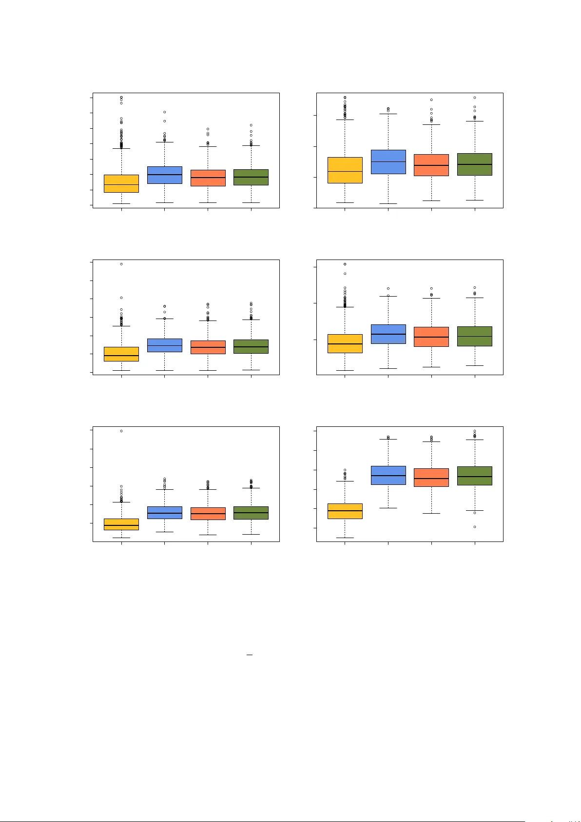
Generalised Exp onen tial Kernels for Nonparametric Densit y Estimation Laura M. Craig ∗ and W agner Barreto-Souza † Scho ol of Mathematics and Statistics, University Col le ge Dublin, Belfield, R epublic of Ir eland F ebruary 18, 2026 Abstract This paper introduces a no v el k ernel densit y estimator (KDE) based on the gen- eralised exp onen tial (GE) distribution, designed specifically for p ositiv e con tinuous data. The prop osed GE KDE offers a mathematically tractable form that a v oids the use of sp ecial functions, for instance, distinguishing it from the widely used gamma KDE, which relies on the gamma function. Despite its simpler form, the GE KDE main tains similar flexibilit y and shape characteristics, aligning with distributions suc h as the gamma, which are kno wn for their effectiv eness in mo delling p ositive data. W e derive the asymptotic bias and v ariance of the proposed k ernel density estimator, and formally demonstrate the order of magnitude of the remaining terms in these expressions. W e also prop ose a second GE KDE, for which w e are able to sho w that it achiev es the optimal mean integrated squared error, something that is difficult to establish for the former. Through numerical exp eriments inv olving sim- ulated and real data sets, we show that GE KDEs can b e an imp ortant alternative and competitive to existing KDEs. Keywor ds : Bandwidth parameter, Bias, Contin uous p ositiv e data, Consistency , Inte- grated mean squared error. 1 In tro duction The classic k ernel density estimator (KDE) used in nonparametric statistics was in tro- duced by Rosen blatt ( 1956 ) and P arzen ( 1962 ) to estimate densit y function with supp ort on the real line R . Let X 1 , . . . , X n b e an iid (indep endent and identically distributed) sample from a distribution with density function f : R → R + ≡ (0 , ∞ ), then the KDE of f assumes the form b f ( x ) = 1 n n X i =1 1 h K  x − X i h  , x ∈ R , ∗ email : laura.craig@ucdconnect.ie † email : w agner.barreto-souza@ucd.ie 1 where K ( · ) is a density (k ernel) function symmetric around zero (for instance, a standard normal one), and h is the bandwidth parameter. Under the conditions that the densit y f is three times differentiable with b ounded third deriv ativ es, and K has finite third momen t, we ha v e that the bias and v ariance of b f are giv en resp ectiv ely by bias  b f ( x )  = 1 2 h 2 f ′′ ( x ) Z ∞ −∞ y 2 K ( y ) dy + o ( h 2 ) , as h → 0, and V ar  b f ( x )  = 1 nh f ( x ) Z ∞ −∞ K 2 ( y ) dy + o  1 nh  , as nh → ∞ ; for instance, see Theorem 6.4.3 from Lehmann ( 1999 ). Since the bias and v ariance form ulas for symmetric kernel density estimators (KDEs) with supp ort on R hold under fairly general assumptions, different kernels tend to p erform similarly . As a result, bandwidth selection is typically more critical than the choice of kernel. KDEs defined on the entire real line R suffer from an issue kno wn as “b oundary bias” when applied to nonnegative data. This arises b ecause the estimator assigns a nonzero probability to negativ e v alues, ev en though the true data are constrained to be nonnegativ e. As a result, densit y estimates near the boundary (i.e., close to zero) b ecome less accurate and more biased ( Chen , 2000 ). Sev eral studies hav e prop osed the use of asymmetric k ernels as a mo dification of the traditional Parzen–Rosen blatt k ernel densit y estimator to b etter accommo date nonnega- tiv e contin uous data. The general form of an asymmetric KDE is b f ( x ) = 1 n n X i =1 K F ( a ( x,b ) ,c ( b )) ( X i ) , where X 1 , . . . , X n are independent and identically distributed (iid) random v ariables with true densit y function f with supp ort on R + , K F ( a ( x,b ) ,c ( b )) ( · ) is an asymmetric kernel from a distribution F parameters with a ( x, b ) and c ( b ) as a function of ( y , b ) and b , resp ectiv ely , and b denotes the smo othing (bandwidth) parameter. One of the first attempts to in tro duce an asymmetric KDE is due to Chen ( 2000 ) with a gamma k ernel given b y K GA ( x/b +1 ,b ) ( z ) = z x/b exp {− z /b } b x/b +1 Γ ( x/b + 1) , z > 0 , whic h will be refereed as Gam1 KDE along with this paper. T o remo v e the dependence of the bias on the first deriv ativ e of f in the in terior (i.e., a w a y from x = 0), Chen ( 2000 ) also prop osed a second gamma kernel given by K GA ( ρ b ( x ) ,b ) ( z ), with ρ b ( x ) = x/b for x ≥ 2 b and ρ b ( x ) = 1 4 ( x/b ) 2 + 1 otherwise. This second gamma KDE will b e refereed as Gam2. Scail- let ( 2004 ) introduced t w o alternativ es to the gamma k ernel based on the in v erse-Gaussian (IG) and recipro cal in v erse-Gaussian (RIG) distributions, with resp ective kernels K I G ( x, 1 /b ) ( z ) = 1 √ 2 π bz 3 exp  − 1 2 bx  z x − 2 + x z   , z > 0 , 2 and K RI G (1 / ( x − b ) , 1 /b ) ( z ) = 1 √ 2 π bz exp  − x − b 2 b  z x − b − 2 + x − b z  , z > 0 . Other asymmetric KDEs hav e b een prop osed based on the lognormal ( Jin and Kaw czak , 2003 ), Birn baum-Saunders ( Jin and Kaw czak , 2003 ; Marchan t et al. , 2013 ; Kakizaw a , 2021 ), in verse gamma ( Kakiza wa and Igarashi , 2017 ), generalised gamma ( Hiruk aw a and Sakudo , 2015 ; Igarashi and Kakizaw a , 2018 ), b eta prime ( Er¸ celik and Nadar , 2020 ), and m ultiv ariate elliptical-based Birn baum-Saunders ( Kakizaw a , 2022 ) distributions. The es- timation of the first-order deriv ative of densit y functions with supp ort on R + has b een recen tly addressed b y F unk e and Hiruk aw a ( 2024 ). Alternativ e metho ds ha ve b een pro- p osed by Geenens and W ang ( 2018 ) and Geenens ( 2021 ) based on the lo cal-lik eliho o d transformation and Mellin-Meijer KDEs, resp ectively . This pap er aims to contribute to the gro wing b o dy of work on asymmetric kernel densit y estimators (KDEs) for p ositiv e contin uous data by introducing a nov el KDE based on the generalised exp onential (GE) distribution. The proposed GE-based k ernel offers a mathematically tractable form, free from sp ecial functions such as the gamma function that is inv olved in the widely used gamma KDE. Despite the gamma KDE’s p opularit y and versatilit y in handling non-negative data, the GE KDE presents a simpler alternativ e while retaining similar flexibility . By lev eraging the prop erties of the GE mo del, whic h shares the same general shape as the density and hazard functions of the gamma distribution, this new k ernel pro vides an efficien t and accessible option for densit y estimation. A second GE KDE is also prop osed, for which w e are able to show that it ac hiev es the optimal mean integrated squared error, something that is difficult to establish for the former. The motiv ation for developing the GE KDEs also lies in the fact that different asym- metric kernels ma y yield distinct asymptotic prop erties for bias and v ariance. This v ari- abilit y highlights the imp ortance of expanding the toolkit of k ernels specifically designed for p ositive data. The GE KDEs provide an app ealing alternativ e for b oth theoretical analysis and practical implementation. This pap er explores their properties, compares their p erformance to existing methods, and argues for their utility as strong comp etitors to existing asymmetric k ernels. W e deriv e the asymptotic bias and v ariance of the pro- p osed kernel density estimators, and formally demonstrate the order of magnitude of the remaining terms in these expressions, whic h is not alwa ys addressed in existing pap ers on the topic. Moreo v er, through numerical exp erimen ts inv olving sim ulated and real data sets, we show that GE KDEs can be an imp ortan t alternativ e and comp etitiv e to existing KDEs. The pap er is organised as follows. Section 2 introduces the generalised exp onential k ernel and provides some theoretical results. Section 3 fo cuses on Monte Carlo exp er- imen ts to compare the finite sample p erformance of the generalised exp onen tial KDE and its existing comp etitors. A second GE KDE is proposed and explored in Section 4 . Section 5 applies the generalised exp onential KDEs to t w o real data sets and compares them to existing KDEs suc h as the gamma ones b y Chen ( 2000 ). Section 6 offers some conclusions on the topic. 3 2 Generalised exp onen tial k ernels The generalised exp onential distribution and its properties ha ve b een studied by Gupta and Kundu ( 2007 ). A generalised exp onential (GE) random v ariable X has a densit y function of the form K GE ( α, 1 /λ ) ( z ) = α λ (1 − exp {− λz } ) α − 1 exp {− λz } , z > 0 , (1) for α, λ > 0. The particular case of in terest here for the first GE KDE is when α > 1, as the densit y function will b e unimo dal. In this case, the mo de is at λ − 1 log α . F or X ∼ GE( α, λ ), the exp ected v alue and v ariance of X are E ( X ) = 1 λ [ ψ ( α + 1) − ψ (1)] and V ar ( X ) = 1 λ 2 [ ψ ′ (1) − ψ ′ ( α + 1)] , where ψ ( z ) = d log Γ( x ) /dx and ψ ′ ( z ) = d 2 log Γ( x ) /dx 2 are the digamma and trigamma functions, resp ectively . The momen t generating function of X , say Φ( t ) = E ( e tX ), as- sumes the form Φ( t ) = Γ( α + 1)Γ(1 − t/λ ) Γ( α − t/λ + 1) , (2) for t < λ ; see Eq. (5) from Gupta and Kundu ( 2007 ). Let X 1 , . . . , X n b e an iid sequence of con tin uous p ositiv e random v ariables with density function f ( x ). W e prop ose our KDE in terms of the K GE ( e x/b ,b ) ( x ) density function, whic h has a mo de at x with bandwidth parameter b = 1 /λ . The first generalised exponential KDE then takes the form b f GE ( x ) = 1 n n X i =1 K GE ( e x/b ,b ) ( X i ) , x > 0 . (3) In what follo ws, we obtain the asymptotic b ehaviour of the bias and v ariance of the prop osed GE KDE for the interior and b oundary x cases, that are resp ectively x/b → ∞ and x/b → c as b → 0, where c is a p ositive real constant. Theorem 2.1. Assume that f ( · ) is a thr e e-times differ entiable function with b ounde d thir d derivative. Then, bias  b f GE ( x )  ≡ E  b f GE ( x )  − f ( x ) = ( bγ f ′ ( x ) + 1 2 ( γ 2 + π 2 / 6) b 2 f ′′ ( x ) + o ( b 2 ) , for x/b → ∞ , b [ ψ ( e c + 1) + γ − c ] f ′ (0) + o ( b ) , for x/b → c, as b → 0 , wher e γ ≈ 0 . 577216 is the Euler’s c onstant. Pr o of. W e hav e that E  b f GE ( x )  = Z ∞ 0 K GE ( e x/b ,b ) ( z ) f ( z ) dz = E ( f ( ζ x )) , (4) 4 where ζ x ∼ GE( e x/b , b ). Let us initially consider the interior x case. W e now expand f ( z ) in T a ylor’s series around µ x ≡ E ( ζ x ) (for instance, see Thm 2.5.1 from Lehmann ( 1999 )): f ( z ) = f ( µ x ) + ( z − µ x ) f ′ ( µ x ) + 1 2 ( z − µ x ) 2 f ′′ ( µ x ) + 1 6 ( z − µ x ) 3 f ′′′ ( ω z ) , (5) where ω z lies b et ween µ x and z . By replacing ( 5 ) in ( 4 ), w e obtain that the bias can b e expressed by bias  b f GE ( x )  = f ( µ x ) − f ( x ) + 1 2 V ar( ζ x ) f ′′ ( µ x ) + 1 6 E  ( ζ x − µ x ) 3 f ′′′ ( ω ζ x )  , (6) with µ x = E ( ζ x ) = b  ψ  e x/b + 1  − ψ (1)  . W e use that ψ ( z ) = log z + O ( z − 1 ) as z → ∞ (for instance, see Sriv astav a and Choi ( 2012 )) and ( e x/b + 1) − 1 = o ( b k ) as b → 0 for an y k ≥ 0 to obtain that µ x = b log( e x/b + 1) + o ( b 2 ) − bψ (1) = x + b log(1 + e − x/b ) + bγ = x + bγ + o ( b 2 ) , (7) where we used that ψ (1) = − γ , with γ denoting the Euler’s constant, and that lim b → 0 log(1 + e − x/b ) /b = − x lim b → 0 1 /b 2 e x/b + 1 = 0 , b y using L’Hopital rule, and therefore b log(1 + e − x/b ) = o ( b 2 ). Hence, by using ( 7 ), it follo ws that f ( µ x ) − f ( x ) = bγ f ′ ( x ) + 1 2 b 2 γ 2 f ′′ ( x ) + o ( b 2 ) . (8) Another term app earing at the bias expression is V ar( ζ x ) = b 2 [ ψ ′ (1) − ψ ′ ( e x/b + 1)] = b 2 [ π 2 / 6 − ψ ′ ( e x/b + 1)]. W e now use that ψ ′ ( z ) = O ( z − 1 ) as z → ∞ (for instance, see Cuyt et al. ( 2008 )) to obtain that V ar( ζ x ) = b 2 π 2 / 6 + o ( b 2 ). Moreov er, f ′′ ( µ x ) = f ′′ ( x ) + O ( b ). Therefore, V ar( ζ x ) f ′′ ( µ x ) = ( b 2 π 2 / 6 + o ( b 2 ))( f ′′ ( x ) + O ( b )) = b 2 π 2 6 f ′′ ( x ) + o ( b 2 ) . (9) W e will now argue that the last term in ( 6 ) is o ( b 2 ). The assumption that the third deriv ativ e of f ( · ) is b ounded, that is, there is M > 0 suc h that | f ′′′ ( z ) | ≤ M for all z , is in force. It follows that | E  ( ζ x − µ x ) 3 f ′′′ ( ω ζ x )  | ≤ E  | ζ x − µ x | 3 | f ′′′ ( ω ζ x ) |  ≤ p E [( ζ x − µ x ) 6 ] q E [ f ′′′ ( ω ζ x ) 2 ] ≤ M p E [( ζ x − µ x ) 6 ] , with Cauch y–Sch warz inequalit y b eing used to obtain the second inequality . W e no w use a result pro vided by Kendall ( 1948 ) (page 63) that expresses the sixth cen tral moments of a random v ariable, sa y µ 6 , in terms of cumulan ts, say κ ′ j s , as follows: µ 6 = κ 6 + 15 κ 4 κ 2 + 10 κ 2 3 + 15 κ 3 2 . (10) 5 The cumulan ts of a random v ariable are obtained b y ev aluating the deriv atives of the cum ulan t generating function (in short, cgf, which is giv en b y the logarithm of the momen t generating function) at zero. By using Eq. ( 2 ), w e obtain that the cgf of ζ x is giv en by C ( t ) ≡ log E ( e tζ x ) = log Γ(1 − tb ) − log Γ( e x/b − tb + 1) + log Γ( e x/b + 1) , t < 1 /b. The j -th cumulan t of ζ x ( κ j ) is given b y κ j = d j C ( t ) dt j     t =0 = ( − 1) j b j  ψ ( j − 1) (1) − ψ ( j − 1) ( e x/b + 1)  , j ≥ 1 , (11) where ψ ( j ) ( z ) = d j − 1 ψ ( z ) /dz j − 1 is the p olygamma function. By using the fact that ψ ( k ) ( z ) = O ( z − k ) for k ≥ 1, and the expression for cum ulants ( 11 ) in ( 10 ), w e immediately obtain that E [( ζ x − µ x ) 6 ] = O ( b 6 ), and therefore E  ( ζ x − µ x ) 3 f ′′′ ( ω ζ x )  = o ( b 2 ) . (12) No w, we use ( 8 ), ( 9 ), and ( 12 ) in ( 6 ) to obtain the desirable result for interior x . F or b oundary x ( x/b → c as b → 0), the bias expression given in ( 6 ) still holds. W e ha v e that f ( µ x ) = f  b  ψ  e x/b + 1  − ψ (1)  = f (0) + b  ψ  e x/b + 1  − ψ (1)  f ′ (0) + o ( b ) and f ( x ) = f (0) + xf ′ (0) + o ( b ) . Hence, f ( µ x ) − f ( x ) = b [ ψ ( e x/b + 1) + γ ] f ′ (0) − xf ′ (0) + o ( b ) = b [ ψ ( e c + 1) + γ − c ] f ′ (0) + o ( b ) , (13) where we ha v e used that x/b → c to obtain the second equalit y . F urther, V ar( ζ x ) f ′′ ( µ x ) = { b 2 [ π 2 / 6 − ψ ′ ( e c + 1)] + o ( b 2 ) }{ f ′′ ( x ) + O ( b ) } = o ( b ) . (14) Finally , the last term of the bias expression is o ( b 2 ) exactly as argued for the interior x case. In other w ords, ( 12 ) still holds. By using ( 13 ), ( 14 ), and ( 12 ) in ( 6 ), we obtain the asymptotic result for the b oundary x case, and this completes the pro of of the theorem. Theorem 2.2. Under the c ondition of The or em 2.1 , for nb → ∞ as b → 0 , the varianc e of the GE KDE is V ar  b f GE ( x )  =        1 4 bn f ( x ) + o  1 nb  , for x/b → ∞ , 1 4 bn e c e c − 1 / 2 f ( x ) + o  1 nb  , for x/b → c. 6 Pr o of. The v ariance of the generalised exp onential KDE is V ar  b f GE ( x )  = 1 n E   K GE ( e x/b ,b ) ( X )  2  + 1 n h E  K GE ( e x/b ,b ) ( X ) i 2 , where X denotes a random v ariable with density function f ( · ). F rom Theorem 2.1 , w e ha v e that E  K GE ( e x/b ,b ) ( X )  = f ( x ) + O ( b ). Therefore, V ar  b f GE ( x )  = 1 n E   K GE ( e x/b ,b ) ( X )  2  + O ( n − 1 ) . (15) The term inv olved in the expectation on the righ t side of ( 15 ) can b e expressed in terms of the b eta exp onential (BE) distribution introduced by Nadara jah and Kotz ( 2006 ). A random v ariable Z follo ws a BE distribution with shap e parameters a, b > 0 and scale parameter λ > 0 if its densit y function assumes the form g B E ( a,b,λ − 1 ) ( z ) = λ B ( a, b ) e − bλz (1 − e − bz ) a − 1 , for z > 0, where B ( a, b ) = Γ( a )Γ( b ) Γ( a + b ) is the b eta function. W e denote Z ∼ BE( a, b, λ − 1 ). It follo ws that E   K GE ( e x/b ,b ) ( X )  2  = e 2 x/b b B (2 e x/b − 1 , 2) E [ f ( η x )] = 1 2 b e x/b 2 e x/b − 1 E [ f ( η x )] , (16) where η x ∼ BE(2 e x/b − 1 , 2 , b ). The mean and the v ariance of η x are given b y µ ∗ x ≡ E ( η x ) = b [ ψ (2 e x/b + 1) − ψ (2)] and V ar( η x ) = b 2 [ ψ ′ (2) − ψ ′ (2 e x/b + 1)]. W e no w expand f ( · ) in T aylor’s series around µ ∗ x and tak e the exp ectation (in a similar fashion as done in Theorem 2.1 ) to obtain that E [ f ( η x )] = f ( µ ∗ x ) + 1 2 V ar( η x ) f ′′ ( µ ∗ x ) + 1 6 E  ( ζ x − µ ∗ x ) 3 f ′′′ ( ω ∗ η x )  , (17) where ω ∗ η x lies b etw een µ ∗ x and η x . W e hav e that µ ∗ x → x as b → 0. Moreo v er, V ar( η x ) = b 2 [ ψ ′ (2) − ψ ′ (2 e x/b + 1)] = o ( b ) and f ′′ ( µ x ) = f ′′ ( x ) + O ( b ) (using similar argumen ts as those from pro of of Theorem 2.1 ) for both in terior and boundary x . So, V ar( η x ) f ′′ ( µ x ) = o ( b ). W e no w claim that E  ( ζ x − µ ∗ x ) 3 f ′′′ ( ω ∗ η x )  = o ( b 2 ). The w a y to justify this result follo ws the same steps as those from Theorem 2.1 , and using the fact that the cum ulan t generating function of η x is given by Φ η x ( t ) ≡ log E ( e tη x ) = log Γ(2 − bt ) − log Γ(2 e x/b − bt + 1) + log Γ(2 e x/b + 1), for t < 2 /b , where w e hav e used Eq. (3.1) from Nadara jah and Kotz ( 2006 ) to get the mgf of a b eta exp onen tial distribution. The cumulan ts of η x are given b y κ j = ( − b ) j { ψ ( j − 1) (2) − ψ ( j − 1) (2 e x/b + 1) } = O ( b j ), whic h holds for b oth interior and b oundary x . 7 Using the ab ov e results, ( 16 ), and ( 17 ) in ( 15 ), w e obtain that V ar  b f GE ( x )  = 1 2 nb e x/b 2 e x/b − 1  f ( µ ∗ x ) + o ( b ) + o ( b 2 )  + O ( n − 1 ) = 1 2 nb e x/b 2 e x/b − 1 f ( µ ∗ x ) + o  1 bn  + O ( n − 1 ) = 1 4 nb e x/b 2 e x/b − 1 [ f ( x ) + O ( b )] + o  1 bn  = 1 4 nb e x/b e x/b − 1 / 2 f ( x ) + o  1 bn  , (18) where we used that f ( µ ∗ x ) = f ( x ) + O ( b ) for b oth interior and b oundary x and that O ( n − 1 ) = o (1 / ( nb )). F rom ( 18 ), the stated expressions for the v ariance under the int erior and b oundary cases are immediately obtained. With the asymptotic mean and v ariance of the GE kernel densit y estimators, we can obtain an expression for the mean squared error (MSE), whic h is MSE  b f GE ( x )  =  bγ f ′ ( x ) + 1 2  γ 2 + π 2 6  b 2 f ′′ ( x ) + o ( b 2 )  2 + 1 4 bn f ( x ) + o  1 nb  = b 3 γ  γ 2 + π 2 6  f ′ ( x ) f ′′ ( x ) + b 2 γ 2 f ′ ( x ) 2 + 1 4 bn f ( x ) + o ( b 3 + ( nb ) − 1 ) , while the mean in tegrated squared error (MISE) is approximately MISE  b f GE ( x )  ≈ b 3 γ  γ 2 + π 2 6  Z ∞ 0 f ′ ( x ) f ′′ ( x ) dx + b 2 γ 2 Z ∞ 0 f ′ ( x ) 2 dx + 1 4 bn , where w e hav e assumed that Z ∞ 0 f ′′ ( x ) 2 dx < ∞ and Z ∞ 0 f ′ ( x ) 2 dx < ∞ (whic h implies that Z ∞ 0 f ′ ( x ) f ′′ ( x ) dx is integrable b y using Cauc h y-Sc hw arz inequality). W e cannot obtain an explicit form for the optimal bandwidth b that minimises the appro ximated MISE, but this can b e done n umerically . Also, the integrals in volv ed in th at expression can b e computed b y replacing the first t wo deriv atives with some estimators or by assuming some true densit y function. In this paper, the rule-of-th um b introduced b y Silverman ( 1986 ) will b e adopted when calculating the bandwidth parameter. 3 Mon te Carlo exp erimen ts T o in v estigate the finite sample properties of our KDE and its comp etitors, sim ulations w ere carried out to compare the MISEs of the GE kernel, the tw o gamma k ernels ( Chen , 2000 ) and the RIG k ernel ( Scaillet , 2004 ) (the IG case was not presen ted since such a k ernel did not pro duce comp etitive results). Fiv e differen t underlying distributions are considered as sho wn in T able 1 , in volving gamma, inv erse gamma, inv erse W eibull, mixture of gamma, mixture of inv erse gamma, and mixture of inv erse W eibull. Tw o 8 sample sizes, n = 100 and n = 500, were considered, and the n umber of Mon te Carlo replications w as 1000. Eac h k ernel is tested on all six of the configurations, and the MISE results are recorded in b o xplots as sho wn in Figures 1 and 2 . Bandwidth was computed using Silverman’s rule-of-th um b ( Silverman , 1986 ). Configuration Distribution A Gamma(25,0.5) B In v erse Gamma(25,150) C In v erse W eibull(5,800) D Gamma Mixture((2/3,1/3), (Γ(25 , 0 . 5), Γ(5 , 2))) E In v erse Gamma Mixture((2/3,1/3), ( I Gam (25 , 150), I Gam (30 , 5))) T able 1: Distributions/configurations used in the Monte Carlo simulation exp erimen ts. F or configurations A, B, and C, the GE MISE v alues are lo w er than those of the Gamma and RIG kernels. The v ariances are similar across all k ernels, and the MISE v alues of the Gamma and RIG kernels are similar. The MISE results for the GE and Gamma k ernels are comp etitive for configurations D and E, sharing a similar v ariance with Gam1 coming in with the lo w est v alues. The RIG results are the largest in b oth magnitude and v ariance. As can be seen from T able 2 , the a v erage MISE v alues resulting from use of the GE k ernel in the simulation scenarios are more often than not the lo w est out of the KDEs presented. Configuration n GE Gam1 Gam2 RIG A 100 1 . 55 × 10 − 5 2 . 01 × 10 − 5 1 . 82 × 10 − 5 1 . 86 × 10 − 5 500 6 . 40 × 10 − 6 7 . 59 × 10 − 6 7 . 07 × 10 − 6 7 . 19 × 10 − 6 B 100 1 . 05 × 10 − 3 1 . 49 × 10 − 3 1 . 40 × 10 − 3 1 . 43 × 10 − 3 500 4 . 64 × 10 − 4 5 . 81 × 10 − 4 5 . 46 × 10 − 4 5 . 54 × 10 − 4 C 100 4 . 96 × 10 − 8 7 . 91 × 10 − 8 7 . 69 × 10 − 8 7 . 90 × 10 − 8 500 3 . 83 × 10 − 8 7 . 47 × 10 − 8 7 . 21 × 10 − 8 7 . 41 × 10 − 8 D 100 3 . 64 × 10 − 4 3 . 63 × 10 − 4 3 . 61 × 10 − 4 3 . 64 × 10 − 4 500 3 . 42 × 10 − 4 3 . 32 × 10 − 4 3 . 29 × 10 − 4 3 . 31 × 10 − 4 E 100 1 . 05 × 10 − 1 9 . 67 × 10 − 2 9 . 95 × 10 − 2 1 . 20 × 10 − 1 500 9 . 95 × 10 − 2 8 . 63 × 10 − 2 9 . 02 × 10 − 2 1 . 08 × 10 − 1 T able 2: Av erage MISE v alues from Mon te Carlo sim ulations based on GE, Gam1, Gam2, and RIG KDEs. 4 An alternativ e GE KDE with optimal MISE W e here propose a second GE KDE with a reparameterised GE distribution in terms of the mean. As a consequence, we will see that the dep endence of the bias on the first-order deriv ativ e of f will b e eliminated, which is commonly desirable. F urthermore, we will explicitly show that this new KDE achiev es the optimal MISE order of O ( n − 4 / 5 ). 9 GE Gam1 Gam2 RIG 0e+00 2e−05 4e−05 6e−05 MISE values f or gamma, n = 100 KDE MISE GE Gam1 Gam2 RIG 0.0e+00 1.0e−05 MISE values f or gamma, n = 500 KDE MISE GE Gam1 Gam2 RIG 0.000 0.002 0.004 0.006 MISE values f or in verse gamma, n = 100 KDE MISE GE Gam1 Gam2 RIG 0.0005 0.0010 0.0015 MISE values f or in verse gamma, n = 500 KDE MISE GE Gam1 Gam2 RIG 5.0e−08 1.5e−07 2.5e−07 MISE values f or in verse weibull, n = 100 KDE MISE GE Gam1 Gam2 RIG 2.0e−08 6.0e−08 1.0e−07 MISE values f or in verse weibull, n = 500 KDE MISE Figure 1: Bo xplots of the MISEs based on the Configurations A, B, and C. The second GE KDE (referred to as GE2 in what follows) is defined by b f GE 2 ( x ) = 1 n n X i =1 K GE ( ν ( x/b ) ,b ) ( X i ) , x > 0 , (19) where we hav e defined ν ( x/b ) = ψ − 1 ( x/b + ψ (1)) − 1, with ψ − 1 ( · ) b eing the in v erse function of ψ ( · ). In terms of R implemen tation in our numerical experiments, w e consider the function idigamma() from the pack age bzinb for the computation of the in verse of the 10 GE Gam1 Gam2 RIG 0.00020 0.00035 MISE values f or gamma mixture, n = 100 KDE MISE GE Gam1 Gam2 RIG 0.00014 0.00020 0.00026 MISE values f or gamma mixture, n = 500 KDE MISE GE Gam1 Gam2 RIG 0.08 0.10 0.12 0.14 MISE values f or in verse gamma mixture, n = 100 KDE MISE GE Gam1 Gam2 RIG 0.08 0.09 0.10 0.11 MISE values f or in verse gamma mixture, n = 500 KDE MISE Figure 2: Bo xplots of the MISEs based on the Configurations D and E. digamma function inv olved in ( 19 )). The exp ected v alue of a GE( ν ( x/b ) , b ) distribution is x . Therefore, GE2 KDE is defined with observ ations as the mean of the kernels, in con trast with the first GE KDE, where the mode is used. The next result pro vides the asymptotic mean and v ariance of the alternative GE k ernel density estimator. Theorem 4.1. Assume that f ( · ) is a thr e e-times differ entiable function with b ounde d thir d derivative. Then, bias  b f GE 2 ( x )  = b 2 π 2 12 f ′′ ( x ) + o ( b 2 ) , as b → 0 . Mor e over, the asymptotic varianc e of b f GE 2 ( x ) assumes the form as that of the estimator b f GE ( x ) pr ovide d in The or em 2.2 . Pr o of. By using results from Issak a ( 2016 ) (who formally prov ed the asymptotic series for the inv erse of the digamma function giv en by Ramanujan), we hav e that ψ − 1 ( z ) = e z + o (1) as z → ∞ . Hence, it follo ws that ν ( x/b ) = e x/b e − γ + o (1), where γ is the Euler’s constan t. In other w ords, the term ν ( x/b ) in v olved in GE2 KDE b ehav es similarly asymptotically (when b → 0) as e x/b used in GE KDE, apart from the constan t e − γ . This implies that the proofs for the asymptotic expressions for the bias and v ariance for the GE2 KDE follo w exactly as those for GE KDE, and therefore, they are omitted. 11 The mean squared error (MSE) of the GE2 KDE is MSE  b f GE 2 ( x )  = b 4 π 4 144 f ′′ ( x ) 2 + 1 4 bn f ( x ) + o ( b 4 + ( nb ) − 1 ) , while the MISE is approximately MISE  b f GE 2 ( x )  ≈ b 4 π 4 144 Z ∞ 0 f ′′ ( x ) 2 dx + 1 4 bn , (20) where we are assuming that Z ∞ 0 f ′′ ( x ) 2 dx < ∞ . In this case, the optimal bandwidth parameter (say b ∗ ) that minimises the appro ximate MISE can b e computed explicitly and is given b y b ∗ =  9 π 4 R ∞ 0 f ′′ ( x ) 2 dx  1 / 5 n − 1 / 5 . (21) Using the optimal bandwidth ( 21 ) in ( 20 ), we obtain that MISE  b f GE 2 ( x )  = O ( n − 4 / 5 ), whic h achiev es the optimal order of existing KDEs such as Gaussian, gamma, IG, and RIG, among others. W e no w pro vide tw o imp ortant remarks. Remark 4.2. Note that the b andwidth p ar ameter b for our GE kernels is c omp ar able in magnitude to the Gaussian b andwidth b , wher e as for the gamma, IG, and RIG kernels, the appr opriate c omp arison is with their squar e d b andwidth, that is, b 2 . Remark 4.3. (Finiteness of inte gr als) The GE2 KDE only r e quir es Z ∞ 0 f ′′ ( x ) 2 dx < ∞ , wher e as GE1 KDE additional ly r e quir es Z ∞ 0 f ′ ( x ) 2 dx < ∞ . T o use the gamma KDEs by Chen ( 2000 ), it is ne c essary that Z ∞ 0 ( xf ′′ ( x )) 2 dx < ∞ and Z ∞ 0 f ′ ( x ) 2 dx < ∞ . On the other hand, the RIG and IG kernels by Sc ail let ( 2004 ) assume that Z ∞ 0 ( xf ′′ ( x )) 2 dx < ∞ and Z ∞ 0 x − 1 / 2 f ( x ) dx < ∞ , and Z ∞ 0  x 3 f ′′ ( x )  2 dx < ∞ and Z ∞ 0 x − 3 / 2 f ( x ) dx < ∞ , r e- sp e ctively. This highlights the imp ortanc e of c onsidering a r ange of KDEs when analysing p ositive data, as differ ent metho ds r ely on differ ent underlying assumptions. Mor e over, our pr op ose d GE kernels, p articularly GE2, r e quir e substantial ly simpler c onditions than those imp ose d by existing KDEs. W e no w conclude this section b y presen ting a small Mon te Carlo with an additional Configuration F inv olving a mixture of inv erse W eibull distributions, more sp ecifically: In v erse W eibull Mixture((2/3,1/3), ( I W (5 , 800), I W (10 , 400))). Figure 3 presents the b o xplots of the MISEs based on Configuration F under GE, GE2, Gam1, Gam2, and RIG kernels. The a v erage MISE v alues are rep orted in T able 3 . These results show that the GE kernels presen t the smallest MISE v alues, with GE2 b eing the b est approac h under the configuration considered for b oth sample sizes n = 100 and n = 500. In the next section, we compare the GE kernels with their comp etitors using tw o real data applications: one in v olving the lifetimes (in years) of retired women with temp orary disabilities enrolled in the Mexican public insurance system who died in 2004, and another based on a sno wfall dataset collected in Grand Rapids in December 1983. 12 GE GE2 Gam1 Gam2 RIG 1.5e−07 2.5e−07 3.5e−07 MISE values f or in verse weib ull mixture, n = 100 KDE MISE GE GE2 Gam1 Gam2 RIG 1.4e−07 1.8e−07 2.2e−07 MISE values f or in verse weib ull mixture, n = 500 KDE MISE Figure 3: Bo xplots of the MISEs based on Configuration F. Configuration n GE GE2 Gam1 Gam2 RIG F 100 2 . 31 × 10 − 7 2 . 22 × 10 − 7 2 . 58 × 10 − 7 2 . 56 × 10 − 7 1 . 22 × 10 − 1 500 1 . 71 × 10 − 7 1 . 62 × 10 − 7 1 . 95 × 10 − 7 1 . 94 × 10 − 7 1 . 08 × 10 − 1 T able 3: Av erage MISE v alues from Mon te Carlo simulation for Configuration F under GE, GE2, Gam1, Gam2, and RIG KDEs. 5 Real data applications This section explores the application of the GE k ernels to tw o real datasets and compares them with the existing comp etitors: Gam1, Gam2, and RIG KDEs. The bandwidth estimate in this section is calculated using Silverman’s rule-of-th um b as b efore (with the dep endence on the sample size matc hing the k ernels’ optimalit y). Cross-v alidation to calculate bandwidth was exp erimented with; ho w ev er, the results yielded were p o or compared to the Silv erman bandwidth choices. Cross-v alidation bandwidth estimates w ere particularly bad for the RIG k ernel. 5.1 Mexican Institute of So cial Securit y data This data w as considered b y Sanhueza et al. ( 2008 ) as an application of a class of inv erse Gaussian t yp e distributions. The data set contains 280 observ ations in the form of the lifetime (in years) of retired w omen with temp orary disabilities incorp orated into the Mexican public insurance system, who died in 2004. The data w as originally provided b y the Mexican Institute of So cial Security . All of the kernels are reasonably smo oth, with the GE k ernels p eaking in the righ t area. The Gamma and RIG k ernels do not peak in quite the right area. The appro ximate MISE w ere 1 . 020 × 10 − 5 , 1 . 015 × 10 − 5 , 3 . 213 × 10 − 5 , 3 . 307 × 10 − 5 , and 3 . 358 × 10 − 5 for the GE, GE2, Gam1, Gam2, and, RIG kernels, resp ectively . The smallest MISE is ac hiev ed by GE2, closely accompanied b y GE. Figure 4 displays the KDEs along with the histogram for the Mexican Institute of So cial Security data. F rom the plot, w e observe that GE and 13 GE2 b etter capture the features of the data. GE exhibits sligh tly more lo cal v ariation, whereas GE2 is smo other while still p eaking at the appropriate p oints. IMSS Data lif etime (in years) Density 20 30 40 50 60 70 80 90 0.00 0.01 0.02 0.03 0.04 GE GE2 GAM2 GAM1 RIG Figure 4: Kernel densit y estimates and histogram for the Mexican Institute of So cial Securit y data. 5.2 Sno w data This data set was analysed by Er¸ celik and Nadar ( 2020 ) to illustrate nonparametric densit y estimation based on the b eta prime kernel. It is a v ailable in the dataset SnowGR as part of the MosaicData pac k age. The data consists of 119 observ ations of snowfall collected in Grand Rapids, MI, in December 1983. The data w as originally obtained from NOAA. All of the k ernels are reasonably smo oth and peak around the right area. How ever, the GE k ernel follows the shape of the data a little more closely than the Gamma and RIG k ernels. The approximate MISE for the snow data were 2 . 630 × 10 − 6 , 4 . 584 × 10 − 6 , 3 . 152 × 10 − 6 , 5 . 000 × 10 − 6 , and 6 . 097 × 10 − 6 resp ectiv ely under the GE, GE2, Gam1, Gam2, and RIG k ernels. The smallest MISE w as achiev ed b y the first GE k ernel, follo w ed 14 b y Gam1 k ernel. Figure 5.2 sho ws the k ernel density estimates alongside the histogram for the snowfall data. As with the previous example, we visually observ e that GE and GE2 b etter capture the data’s features. GE displays sligh tly more lo cal v ariation, while GE2 remains smo other, y et still p eaks at the appropriate p oin ts. Snow Data snow (in inches) Density 0 10 20 30 40 50 60 0.00 0.02 0.04 GE GE2 GAM2 GAM1 RIG Figure 5: Kernel density estimates and histogram for the snow data. 6 Concluding remarks This pap er introduced a new asymmetric kernel densit y estimator for p ositiv e contin uous data based on the generalised exp onential (GE) distribution. By exploiting the tractable structure of the GE model, the prop osed KDE av oids the use of sp ecial functions suc h as the gamma function required by the gamma KDE, while preserving comparable flexibilit y in shap e and behaviour. As a result, the GE KDE offers a simpler y et effectiv e alterna- tiv e for densit y estimation on the p ositiv e real line, with adv an tages for b oth analytical deriv ations and practical implemen tation. Bey ond its computational simplicit y , the GE KDE enric hes the class of asymmetric kernels av ailable for p ositiv e data, an imp ortant 15 consideration giv en that differen t kernels can exhibit distinct asymptotic bias and v ari- ance prop erties. W e pro vide a detailed theoretical analysis of the prop osed estimator, deriving explicit expressions for its asymptotic bias and v ariance and formally establish- ing the order of the remaining terms. This level of rigor addresses gaps in the existing literature, where suc h remainder terms are not alw ays fully c haracterised. A second GE k ernel was also in tro duced, and w e sho w that it ac hiev es the optimal mean in tegrated squared error, an optimalit y result that could not b e established for the first GE kernel. The practical relev ance of the GE KDEs is further supp orted by numerical studies using simulated and real data sets, whic h demonstrate that the prop osed estimator p er- forms comp etitiv ely with well-established asymmetric KDEs. These results underscore the v alue of expanding the range of k ernels tailored to p ositive data and illustrate that simple distributional choices can yield estimators with strong theoretical and empirical p erformance. Ov erall, the GE KDEs constitute a meaningful addition to the asymmetric KDE framew ork, offering a balance b etw een mathematical tractability , theoretical robustness, and practical effectiv eness. F uture researc h ma y explore data-driv en bandwidth selection, extensions to m ultiv ariate settings, and applications in domains where p ositive-v alued data are prev alent. Ac kno wledgemen ts This publication has emanated from researc h conducted with the financial supp ort of T aighde ´ Eireann – Research Ireland under Grant 18/CR T/6049. F or the purp ose of Op en Access, the authors ha v e applied a CC BY public copyrigh t licence to an y Author Accepted Manuscript v ersion arising from this submission. References Chen, S. X. (2000). Probabilit y densit y function estimation using gamma k ernels. Annals of the Institute of Statistic al Mathematics , 52:471–480. Cuyt, A., P etersen, V. B., V erdonk, B., W aadeland, H., and Jones, W. B. (2008). Hand- b o ok of Continue d F r actions for Sp e cial F unctions . Springer. Er¸ celik, E. and Nadar, M. (2020). Nonparametric densit y estimation based on b eta prime k ernel. Communic ations in Statistics - The ory and Metho ds , 49:325–342. F unke, B. and Hiruk a w a, M. (2024). Densit y deriv ative estimation using asymmetric k ernels. Journal of Nonp ar ametric Statistics , 36:994–1017. Geenens, G. (2021). Mellin–Meijer kernel densit y estimation on R + . Annals of the Institute of Statistic al Mathematics , 73:953–977. Geenens, G. and W ang, C. (2018). Lo cal-likelihoo d transformation kernel density estima- tion for p ositive random v ariables. Journal of Computational and Gr aphic al Statistics , 27:822–835. 16 Gupta, R. D. and Kundu, D. (2007). Generalized exp onen tial distribution: Existing results and some recent dev elopments. Journal of Statistic al Planning and Infer enc e , 137:3537–3547. Hiruk a w a, M. and Sakudo, M. (2015). F amily of the generalised gamma k ernels: a gener- ator of asymmetric k ernels for nonnegativ e data. Journal of Nonp ar ametric Statistics , 27:41–63. Igarashi, G. and Kakizaw a, Y. (2018). Generalised gamma kernel densit y estimation for nonnegativ e data and its bias reduction. Journal of Nonp ar ametric Statistics , 30:598– 639. Issak a, A. (2016). On Ramanujan’s inv erse digamma approximation. The R amanujan Journal , 39:291–302. Jin, X. and Kaw czak, J. (2003). Birnbaum-Saunders and lognormal k ernel estimators for mo delling durations in high frequency financial data. Annals of Ec onomics and Financ e , 4:103–124. Kakiza w a, Y. (2021). A class of Birn baum-Sauders t yp e kernel density estimators for nonnegativ e data. Computational Statistics and Data A nalysis , 161:107249. Kakiza w a, Y. (2022). Multiv ariate elliptical-based Birnbaum–Saunders kernel density estimation for nonnegative data. Journal of Multivariate Analysis , 187:104834. Kakiza w a, Y. and Igarashi, G. (2017). Inv erse gamma k ernel density estimation for nonnegativ e data. Journal of the Kor e an Statistic al So ciety , 46:194–207. Kendall, M. (1948). A dvanc e d The ory of Statistics: V olume 1 . Griffin, 4th edition. Lehmann, E. (1999). Elements of L ar ge-Sample The ory . Springer, 1st edition. Marc han t, C., Bertin, K., Leiv a, V., and Saulo, H. (2013). Generalized Birn- baum–Saunders k ernel density estimators and an analysis of financial data. Com- putational Statistics and Data A nalysis , 63:1–15. Nadara jah, S. and Kotz, S. (2006). The b eta exponential distribution. R eliability Engi- ne ering and System Safety , 91:689–697. P arzen, E. (1962). On estimation of a probabilit y densit y function and mo de. The Annals of Mathematic al Statistics , 33:1065–1076. Rosen blatt, M. (1956). Remarks on some nonparametric estimates of a densit y function. The Annals of Mathematic al Statistics , 27:832–837. Sanh ueza, A., Leiv a, V., and Balakrishnan, N. (2008). A new class of inv erse gaussian t yp e distributions. Metrika , 68:31–49. Scaillet, O. (2004). Density estimation using in v erse and recipro cal inv erse gaussian k ernels. Journal of Nonp ar ametric Statistics , 16:217–266. 17 Silv erman, B. W. (1986). Density Estimation for Statistics and Data Analysis . Chapman and Hall, 1st edition. Sriv asta v a, H. M. and Choi, J. (2012). Zeta and q-Zeta F unctions and Asso ciate d Series and Inte gr als . Elsevier. 18