Space-filling lattice designs for computer experiments
This paper investigates the construction of space-filling designs for computer experiments. The space-filling property is characterized by the covering and separation radii of a design, which are integrated through the unified criterion of quasi-unif…
Authors: Naoki Sakai, Takashi Goda
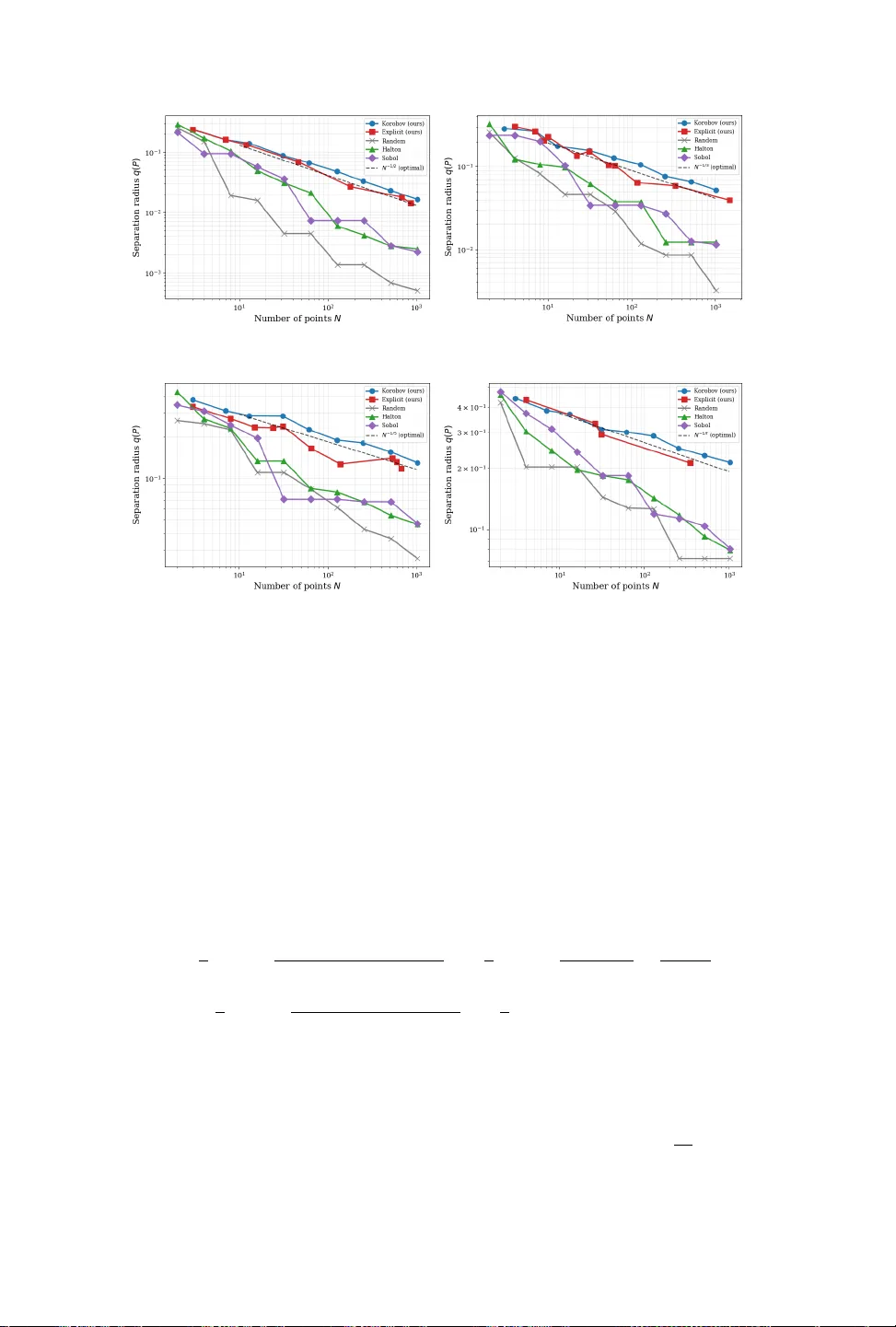
SP A CE-FILLING LA TTICE DESIGNS F OR COMPUTER EXPERIMENTS ∗ NAOKI SAKAI † AND T AKASHI GODA ‡ Abstract. This paper inv estigates the construction of space-filling designs for computer exper- iments. The space-filling prop erty is c haracterized b y the cov ering and separation radii of a design, which are integrated through the unified criterion of quasi-uniformity . W e fo cus on a sp ecial class of designs, known as quasi-Monte Carlo (QMC) lattice p oint sets, and prop ose two construction algo- rithms. The first algorithm generates rank-1 lattice p oint sets as an approximation of quasi-uniform Kroneck er sequences, where the generating vector is determined explicitly . As a byproduct of our analysis, we prov e that this explicit p oint set achiev es an isotropic discrepancy of O ( N − 1 /d ). The second algorithm utilizes Korob ov lattice p oint sets, employing the Lenstra–Lenstra–Lov´ asz (LLL) basis reduction algorithm to identify the generating vector that ensures quasi-uniformity . Numerical experiments are pro vided to v alidate our theoretical claims regarding quasi-uniformity . F urthermore, we conduct empirical comparisons b etw een v arious QMC p oint sets in the con text of Gaussian process regression, show casing the efficacy of the prop osed designs for computer exp eriments. Key w ords. designs of computer exp eriments, quasi-Monte Carlo, quasi-uniformity , geometry of num b ers, successive minima, lattice basis reduction MSC co des. Primary 62K05; Secondary 11H31, 52C17, 65D05, 65D12 1. Introduction. In the field of computer exp eriments, maximin and minimax distance-based designs ha ve gained prominence due to their sup erior space-filling prop- erties [ 8 , 16 , 17 , 18 , 31 , 35 ]. Conceptually , maximin designs prioritize the separation b et ween sampling p oints to ensure that they are well-dispersed across the domain, while minimax designs aim to cov er the target space as efficiently as p ossible by mini- mizing the largest unexplored regions. These t w o geometric ob jectiv es, i.e., separation and co verage, are naturally unified by the concept of quasi-uniformity , which aims to attain b oth prop erties simultaneously and has b ecome one of the cen tral criteria for assessing the qualit y of exp erimen tal designs recently [ 32 , 33 ]. The utilit y of quasi-uniform designs extends across v arious n umerical framew orks, including radial basis function approximation, kernel in terp olation, and Gaussian pro cess regression [ 36 , 37 , 44 , 45 , 46 , 47 ]. T o appreciate the necessity of quasi- uniformit y , consider k ernel in terpolation with standard Sobolev kernels as a primary example. In this context, the geometric prop erties of the p oint set dictate b oth the appro ximation accuracy and the n umerical stabilit y . When the target function resides within the asso ciated native repro ducing kernel Hilb ert space, the appro ximation er- ror is typically b ounded by a p o wer of the co v ering radius. Ho wev er, minimizing the co vering radius is not the sole ob jective. The separation radius is equally critical, as it gov erns the condition n umber of the kernel matrix (Gram matrix); a shrinking separation radius leads to severe ill-conditioning, compromising numerical stabilit y [ 36 ]. F urthermore, in scenarios where the target function possesses low er regularit y than the kernel implies, i.e., when appro ximating a “rough” function that lies out- side the nativ e space, theoretical error bounds often explicitly depend on the mesh ratio (the ratio of the cov ering radius to the separation radius), rather than solely on ∗ Submitted to the editors DA TE. † Department of Energy Science and Engineering, Stanford Universit y , 537 Panama Mall, Stanford, CA 94305, USA ( naoki65@stanford.edu ). ‡ Graduate School of Engineering, The University of T okyo, 7-3-1 Hongo, Bunkyo-ku, T okyo 113- 8656, Japan ( go da@frcer.t.u-tokyo.ac.jp ). 1 2 N. SAKAI AND T. GODA the cov ering radius [ 37 , 44 , 47 ]. Consequently , constructing quasi-uniform designs for computer exp eriments is critical for achieving a balance b etw een high-fidelity conv er- gence and numerical stability . F urthermore, in the context of Bay esian optimization, whic h frequently employs Gaussian pro cess regression as a surrogate model, the use of quasi-uniform designs in the initial sampling stage has empirically b een shown to accelerate the con v ergence of the optimization pro cess [ 19 ]. Quasi-Mon te Carlo (QMC) point sets and sequences, also known as lo w- discrepancy point sets and sequences, are widely recognized for their ab ility to ac hieve faster con vergence rates in numerical integration ov er the unit hypercub e [0 , 1] d than random sampling [ 7 , 20 , 30 ]. Giv en their excellent equi-distribution prop erties, they ha ve also b een considered prime candidates for space-filling quasi-uniform designs, see, for instance, [ 47 , Section 3.1]. How ev er, the sp ecific geometric prop erty of quasi- uniformit y in the QMC context has remained relatively under-explored until very re- cen tly . Recent studies hav e b egun to fill this gap, revealing highly non-trivial results: man y widely used QMC sequences—including the t w o-dimensional Sobol’, F aure, and Halton sequences—fail to satisfy the requirements for quasi-uniformit y (see [ 13 ], [ 5 ], and [ 14 ], resp ectively). More precisely , the separation radius of these sequences deca ys at a faster rate than N − 1 /d , violating the conditions necessary for quasi-uniformity . In contrast, a recent w ork [ 4 ], together with a prior work [ 12 ], pro v es that lattice p oin t sets and Kroneck er sequences can ac hieve quasi-uniformity , provided that their underlying parameters are appropriately selected. While [ 4 ] provided an explicit construction for quasi-uniform Kroneck er sequences, the results for lattice p oint sets remained purely existen tial; neither an explicit con- struction nor a constructiv e algorithm was previously known. Addressing this gap is the primary ob jective of the presen t work. In this paper, w e prop ose tw o dis- tinct metho dologies for constructing space-filling, quasi-uniform lattice designs for computer exp eriments as follows: 1. Explicit r ank-1 lattic e c onstruction : W e pro vide an explicit rank-1 lattice p oin t set construction as a discrete appro ximation of the quasi-uniform Kron- ec ker sequences in tro duced in [ 4 ]. A characteristic of this metho d is that the n umber of sampling p oints N is not arbitrarily chosen but is determined b y the Diophantine prop erties of the parameters defining the underlying Kron- ec ker sequence. Despite this constraint, the metho d provides the parameters, i.e., the generating v ectors, for rank-1 lattice p oin t sets explicitly . F urther- more, this result yields rank-1 lattice p oint sets with low isotropic discrepancy , thereb y pro viding a partial solution to an op en problem regarding the explicit construction of suc h sets [ 6 , Corollary 5.27]. 2. Algorithmic Kor ob ov lattic e c onstruction : F o cusing on a class of Korobov lattice p oint sets, we develop a constructive algorithm that leverages the Lenstra–Lenstra–Lo v´ asz (LLL) lattice basis reduction algorithm [ 25 ] to ef- ficien tly identify the generating vector that ensures quasi-uniformity . This algorithm is applicable for any prime num be r N , and its computational cost is highly efficient, growing at most p olynomially in the dimension d and only quasi-linearly in N . The rest of this pap er is organized as follows. In section 2 , we introduce the nec- essary notation and formal definitions, including the criteria for quasi-uniformity and the construction of QMC lattice p oin t sets. W e also in tro duce the concept of succes- siv e minima from the geometry of n umbers [ 3 , 40 ], and establish their connection to the quasi-uniformity of lattice designs. In section 3 , w e detail our tw o prop osals for constructing space-filling lattice designs: explicit rank-1 lattice construction and al- SP ACE-FILLING LA TTICE DESIGNS 3 gorithmic Korob o v lattice construction. W e provide theoretical results demonstrating that b oth approaches yield quasi-uniform designs. Finally , section 4 presents numeri- cal results and p erformance ev aluations in the context of Gaussian pro cess regression, follo wed by concluding remarks in section 5 . 2. Preliminaries. Throughout this pap er, let Z be the set of in tegers, and N b e the set of p ositive in tegers. W e also use the standard asymptotic notation: for t wo non-negative functions f , g , we write f ( N ) = O ( g ( N )) (resp. f ( N ) = Ω( g ( N ))) if f ≤ C g (resp. f ≥ C g ) for some constant C > 0 and sufficien tly large N , and w e write f ( N ) = Θ( g ( N )) if b oth conditions hold. W e fo cus on the d -dimensional unit cub e [0 , 1] d as our target domain. This choice is without loss of generality: while practical applications often inv olv e general rec- tangular domains, any such domain can b e mapp ed from [0 , 1] d via a linear transfor- mation. Since suc h transformations only alter the cov ering and separation radii by a constan t factor determined b y the domain’s side lengths, the asymptotic properties and the quasi-uniformit y of the designs are preserved. 2.1. Quasi-uniform designs. Let P N ⊂ [0 , 1] d b e a set of N p oints. T o ev aluate ho w w ell these p oints fill the space, w e consider the cov ering radius and the separation radius. The c overing r adius , or fill distance, of P N with resp ect to [0 , 1] d is defined as h ( P N ) = sup x ∈ [0 , 1] d min y ∈ P N ∥ x − y ∥ 2 , whic h measures the largest distance from an y p oint in the domain to the nearest point in P N . The sep ar ation r adius of P N is defined as q ( P N ) = 1 2 min x , y ∈ P N x = y ∥ x − y ∥ 2 , represen ting half the minimum distance b etw een any tw o distinct p oints in the set. These t wo quantities admit the follo wing geometric interpretations. If w e consider Euclidean balls of radius r cen tered at each point in P N , the cov ering radius h ( P N ) is the minimum radius suc h that the union of the closed balls cov ers the entire domain [0 , 1] d . Conv ersely , the separation radius q ( P N ) is the maximum radius such that the in teriors of the balls are pairwise disjoint. F rom these interpretations, it follo ws that for an y set of N p oints P N , there exist p ositive constants C 1 ,d , C 2 ,d , dep ending only on the dimension d , suc h that h ( P N ) ≥ C 1 ,d N − 1 /d and q ( P N ) ≤ C 2 ,d N − 1 /d , (2.1) resp ectiv ely (see, for instance, [ 4 , 5 , 33 ]). Let S ⊂ [0 , 1] d b e an infinite sequence of points, and let P N denote the set consisting of the first N p oints of S . W e formally define the quasi-uniformity of the sequence S as follows. Definition 2.1. An infinite se quenc e of p oints S is quasi-uniform over [0 , 1] d if ther e exists a p ositive c onstant C d , indep endent of N , such that ρ ( P N ) := h ( P N ) q ( P N ) ≤ C d , (2.2) for any N ≥ 2 . The quantity ρ ( P N ) is r eferr e d to as the mesh ratio of P N with r esp e ct to [0 , 1] d . 4 N. SAKAI AND T. GODA As a consequence of the bounds ( 2.1 ), for a quasi-uniform sequence, b oth the cov- ering and separation radii must satisfy h ( P N ) = Θ( N − 1 /d ) and q ( P N ) = Θ( N − 1 /d ). This implies that a quasi-uniform sequence fills the space at the optimal rate while main taining a minim um separation b etw een p oints, also at the optimal rate. W e also define quasi-uniformit y for a sequence of (not necessarily extensible) p oint sets. It was shown in [ 4 , 5 ] that if the condition ( 2.2 ) is satisfied along a subsequence of sample sizes N 1 < N 2 < · · · such that N i +1 ≤ cN i for some constant c > 1, the underlying space-filling prop erty is essentially preserved for all N . Motiv ated by this observ ation, w e adopt the following definition: Definition 2.2. L et ( P N i ) i ∈ N b e a set of p oint sets such that P N i ⊂ [0 , 1] d , wher e N i = | P N i | denotes the numb er of p oints in the i -th set, and N i < N i +1 ≤ cN i for a c onstant c > 1 . If ther e exists a p ositive c onstant C d , indep endent of i , such that ρ ( P N i ) ≤ C d holds for al l i ∈ N , we say that ( P N i ) i ∈ N is a quasi-uniform family of p oint sets. 2.2. Lattices. A lattic e Λ ⊂ R d is a discrete additive subgroup of R d . A full rank lattice is a lattice Λ that can b e represented as the set of all in teger linear com binations of d linearly indep enden t vectors: Λ = T Z d = T k | k ∈ Z d , where T ∈ R d × d is an in vertible matrix called the gener ating matrix (or b asis matrix ). The columns of T form a basis of the lattice. W e define the co vering and separation radii of Λ with respect to the Euclidean space R d b y h (Λ) := sup x ∈ R d min y ∈ Λ ∥ x − y ∥ 2 , and q (Λ) := 1 2 min x , y ∈ Λ x = y ∥ x − y ∥ 2 = 1 2 min x ∈ Λ \{ 0 } ∥ x ∥ 2 , resp ectiv ely . Lik ewise, the mesh ratio is defined by ρ (Λ) := h (Λ) /q (Λ). The separation radius q (Λ) is equiv alen t to half the length of the shortest non-zero vector in the lattice. F or a giv en num b er of p oin ts N and a generating vector z = ( z 1 , . . . , z d ) ∈ { 1 , . . . , N − 1 } d , let us consider the set P N , z := n x n = n nz 1 N o , . . . , n nz d N o | n = 0 , 1 , . . . , N − 1 o ⊂ [0 , 1] d , whic h is called a r ank-1 lattic e p oint set , where { x } = x − ⌊ x ⌋ denotes the fractional part of x . This p oint set has b een extensiv ely studied in the con text of QMC inte- gration [ 6 , 30 , 41 ]. Throughout this pap er, we assume gcd( N , z 1 , . . . , z d ) = 1, whic h ensures that P N , z consists of N distinct p oin ts. Suc h a p oint set can be viewed as the in tersection P N , z = Λ ∩ [0 , 1) d with an infinite lattice Λ = 1 N z Z + Z d . Since Z d ⊆ Λ and the unit cub e [0 , 1) d con tains exactly N distinct p oints of Λ under the condition gcd( N , z 1 , . . . , z d ) = 1, the volume of the fundamental domain of Λ is 1 / N . Therefore, there alw a ys exists a generating matrix T ∈ R d × d for Λ suc h that det( T ) = 1 / N . F or instance, when gcd( N , z 1 ) = 1, a generating matrix T can b e explicitly constructed as T = 1 / N 0 . . . 0 z − 1 1 z 2 / N 1 . . . 0 . . . . . . . . . . . . z − 1 1 z d / N 0 . . . 1 , (2.3) SP ACE-FILLING LA TTICE DESIGNS 5 where z − 1 1 ∈ Z N is the multiplicativ e in v erse of z 1 mo dulo N . More generally , for an y z with at least one comp onent coprime to N , w e can achiev e gcd( N , z 1 ) = 1 by reordering coordinates, allowing us to use this explicit form. A w ell-known sp ecial case is the Kor ob ov lattic e p oint set , where z = (1 , a, a 2 , . . . , a d − 1 ) (mod N ) for some in teger a ∈ Z N , which alwa ys satisfies gcd( N , z 1 ) = 1. R emark 2.3. It should b e noted that the term “rank-1” refers to the fact that a single v ector z generates P N , z as a finite ab elian group (sp ecifically , P N , z ∼ = Z N when gcd( N , z 1 , . . . , z d ) = 1). This is distinct from the rank of the underlying infinite lattice Λ ⊂ R d , which is d (full rank) since its generating matrix T is in vertible. The dual lattice of Λ, which plays an important role in the subsequen t analysis, is defined b y Λ ⊥ := y ∈ R d | x · y ∈ Z for all x ∈ Λ . Let T b e a generating matrix for Λ. Then, it is easily seen that the dual lattice Λ ⊥ itself is also a lattice and that its generating matrix is ( T − 1 ) ⊤ . In particular, if T is giv en by ( 2.3 ), the generating matrix for Λ ⊥ is ( T − 1 ) ⊤ = N − z − 1 1 z 2 . . . − z − 1 1 z d 0 1 . . . 0 . . . . . . . . . . . . 0 0 . . . 1 (mo d N ) , (2.4) for which det(( T − 1 ) ⊤ ) = N holds. 2.3. Successive minima and quasi-uniformity . T o further characterize the geometry of a lattice Λ, we introduce the concept of suc c essive minima from the geometry of n umbers [ 3 , 40 ]. F or j = 1 , . . . , d , the j -th successive minimum of Λ with resp ect to the Euclidean ball B d := x ∈ R d | ∥ x ∥ 2 ≤ 1 is defined as λ j (Λ) := inf { r > 0 | dim(span(Λ ∩ r B d )) ≥ j } . By definition, λ j (Λ) represents the radius of the smallest ball centered at the origin that contains j linearly independent lattice vectors. The successive minima are closely related to the cov ering and separation radii of the lattice. F rom the definition of q (Λ) in subsection 2.2 , it immediately follo ws that q (Λ) = λ 1 (Λ) 2 . Regarding the co v ering radius of the lattice, it is known that 1 2 λ d (Λ) ≤ h (Λ) ≤ √ d 2 λ d (Λ) , see, for instance, [ 27 , Theorem 7.9]. Moreov er, in [ 1 ], Banaszczyk prov ed the following transference theorems: 1 2 ≤ h (Λ) λ 1 (Λ ⊥ ) ≤ d 2 and 1 ≤ λ j (Λ) λ d − j +1 (Λ ⊥ ) ≤ d, (2.5) 6 N. SAKAI AND T. GODA for all j = 1 , . . . , d . These b ounds imply that the mesh ratio ρ (Λ) is fundamentally c haracterized by the balance of successive minima: max λ d (Λ) λ 1 (Λ) , d − 1 λ d (Λ ⊥ ) λ 1 (Λ ⊥ ) ≤ ρ (Λ) ≤ min √ d λ d (Λ) λ 1 (Λ) , d λ d (Λ ⊥ ) λ 1 (Λ ⊥ ) . (2.6) This sandwiching of ρ (Λ) shows that the mesh ratio is small if and only if the successiv e minima of the lattice (or its dual lattice) are well-balanced. Applying Minko wski’s second theorem, we obtain the following result: Lemma 2.4. L et Λ ⊂ R d b e a lattic e with a gener ating matrix T , and Λ ⊥ b e its dual lattic e. Then, ρ (Λ) ≤ C d min √ d | det( T ) | ( λ 1 (Λ)) d , d | det( T − 1 ) | ( λ 1 (Λ ⊥ )) d , with C d = 2 d Γ(1 + d/ 2) /π d/ 2 wher e Γ denotes the gamma function. Pr o of. Minko wski’s second theorem states that d Y j =1 λ j (Λ) ≤ 2 d Γ(1 + d/ 2) π d/ 2 | det( T ) | , see [ 3 , 40 ]. Since the successive minima are ordered, i.e., λ 1 (Λ) ≤ λ 2 (Λ) ≤ · · · ≤ λ d (Λ), w e obtain λ d (Λ) ≤ 2 d Γ(1 + d/ 2) π d/ 2 | det( T ) | d − 1 Y j =1 1 λ j (Λ) ≤ 2 d Γ(1 + d/ 2) π d/ 2 | det( T ) | ( λ 1 (Λ)) d − 1 . Similarly , for the dual lattice Λ ⊥ , we hav e λ d (Λ ⊥ ) ≤ 2 d Γ(1 + d/ 2) π d/ 2 det( T − 1 ) d − 1 Y j =1 1 λ j (Λ ⊥ ) ≤ 2 d Γ(1 + d/ 2) π d/ 2 det( T − 1 ) ( λ 1 (Λ ⊥ )) d − 1 . By applying these estimates to the upp er b ound in ( 2.6 ), we obtain the desired in- equalit y . R emark 2.5. The recipro cal of the length of the shortest non-zero v ector in the dual lattice, 1 /λ 1 (Λ ⊥ ), is called the sp e ctr al test , which is a standard quality measure for linear congruential pseudo-random num ber generators [ 23 , 24 ]. In that context, 1 /λ 1 (Λ ⊥ ) represents the maximum distance b etw een adjacent parallel hyperplanes that co ver all lattice p oints. A larger λ 1 (Λ ⊥ ) corresp onds to a smaller distance b e- t ween these hyperplanes, indicating a more “uniform” distribution of p oints. The ab o ve lemma pro vides a theoretical bridge betw een this classical metric and the space- filling prop erty . Before moving on to the next section, we sho w that the mesh ratio of the p oin t set P = Λ ∩ [0 , 1) d with respect to [0 , 1] d is bounded by the mesh ratio of the lattice Λ with resp ect to R d , up to a constant factor. Although a similar result was prov en in [ 4 ], our argument b elow directly deals with the Euclidean norm, instead of the ℓ ∞ -norm as considered in [ 4 ]. SP ACE-FILLING LA TTICE DESIGNS 7 Lemma 2.6. L et Λ ⊂ R d b e a lattic e and P = Λ ∩ [0 , 1) d , Assume | P | ≥ 2 . The sep ar ation and c overing r adii of P with r esp e ct to [0 , 1] d satisfy q ( P ) ≥ q (Λ) and h ( P ) ≤ ( 2 √ d h (Λ) if h (Λ) ≥ 1 / 2 , (1 + √ d ) h (Λ) otherwise. Conse quently, the mesh r atio of P is b ounde d by ρ ( P ) ≤ ( 2 √ d ρ (Λ) if h (Λ) ≥ 1 / 2 , (1 + √ d ) ρ (Λ) otherwise. . Pr o of. The inequality q ( P ) ≥ q (Λ) follows immediately from the fact that P ⊂ Λ. F or the cov ering radius, let us write ϵ := h (Λ). If ϵ ≥ 1 / 2, the result is clear as w e hav e h ( P ) ≤ diam([0 , 1] d ) = √ d ≤ 2 √ d ϵ. Assume ϵ < 1 / 2. F or an y x ∈ [0 , 1] d , we can choose a “shifted center” z ∈ [ ϵ, 1 − ϵ ] d suc h that the Euclidean ball B ( z , ϵ ) = { y ∈ R d | ∥ y − z ∥ 2 ≤ ϵ } is contained in [0 , 1] d . Sp ecifically , w e set z j = ϵ if x j < ϵ , 1 − ϵ if x j > 1 − ϵ , x j otherwise, for each j = 1 , . . . , d . By the definition of h (Λ), there exist a lattice p oint y ∗ ∈ Λ suc h that ∥ y ∗ − z ∥ 2 ≤ ϵ . Since we hav e B ( z , ϵ ) ⊂ [0 , 1] d , it follo ws that y ∗ ∈ P . Now, w e ev aluate the distance b etw een x and y ∗ . By the triangle inequalit y , it holds that ∥ x − y ∗ ∥ 2 ≤ ∥ x − z ∥ 2 + ∥ z − y ∗ ∥ 2 ≤ ∥ x − z ∥ 2 + ϵ. F rom the definition of z , w e ha v e | x j − z j | ≤ ϵ for all j , whic h implies ∥ x − z ∥ 2 ≤ √ dϵ . Thus, ∥ x − y ∗ ∥ 2 ≤ (1 + √ d ) ϵ . Since this holds for any x ∈ [0 , 1] d , we obtain h ( P ) ≤ (1 + √ d ) h (Λ). The b ound on the mesh ratio for P follo ws immediately . This lemma guaran tees that finding a lattice Λ with a small mesh ratio ρ (Λ) is sufficien t to construct a quasi-uniform p oint set P . Combining this with Lemma 2.4 , our goal reduces to finding a generating vector z that maximizes λ 1 (Λ) or λ 1 (Λ ⊥ ). R emark 2.7. F or any fixed shift ∆ ∈ R d , consider the shifted lattice Λ ∆ := Λ + ∆ and the corresp onding finite p oint set P ∆ = Λ ∆ ∩ [0 , 1) d . Since the cov ering and separation radii of a lattice are inv ariant under translation, w e hav e h (Λ ∆ ) = h (Λ) and q (Λ ∆ ) = q (Λ). Thus, provided | P ∆ | ≥ 2, the b ounds in the ab ov e lemma remain v alid for the shifted p oint set P ∆ : ρ ( P ∆ ) ≤ ( 2 √ d ρ (Λ) if h (Λ) ≥ 1 / 2, (1 + √ d ) ρ (Λ) otherwise. 3. Construction of space-filling lattice designs. Based on the theoretical results in the previous section, our goal is to find a generating vector z that makes λ 1 (Λ) (or λ 1 (Λ ⊥ )) as large as possible. 8 N. SAKAI AND T. GODA 3.1. Explicit rank-1 lattice construction. F or d = 2, the Fib onacci lattice with N = F m and z = (1 , F m − 1 ) is a known explicit construction that achiev es quasi- uniformit y [ 4 ]. F or d ≥ 3, how ev er, no explicit construction of go o d generating v ectors is known so far. This problem is partly addressed in this subsection. Let α = ( α 1 , . . . , α d ) ∈ R d b e a fixed v ector. Consider an infinite sequence of p oints of the form S = ( { n α } ) n ≥ 1 , called the Kr one cker se quenc e . In [ 4 ], it is pro ven that the Kronec k er sequence is quasi-uniform if 1 , α 1 , . . . , α d ∈ R are linearly indep enden t elements of an algebraic extension of the rational field Q of degree d + 1. Th us, for instance, if α = p 1 / ( d +1) , p 2 / ( d +1) , . . . , p d/ ( d +1) , (3.1) for a prime num ber p , the corresp onding Kroneck er sequence is quasi-uniform. The pro of relies on appro ximating the initial segmen t of the Kronec k er sequence by a rank-1 lattice point set. A similar proof technique was originally emplo yed b y Larc her [ 21 ], who pro v ed that such Kroneck er sequences achiev e an isotropic discrepancy of O ( N − 1 /d ). It turns out that this appro ximation provides an explicit construction of go o d generating vectors, b oth in terms of quasi-uniformity and isotropic discrepancy . Our construction metho d pro ceeds as follows: Algorithm 3.1 Explicit construction of rank-1 lattices via algebraic num bers Require: Dimension d ≥ 1, algebraic vector α ∈ R d suc h that { 1 , α 1 , . . . , α d } is linearly indep endent ov er Q and spans an algebraic extension of degree d + 1. 1: Set N 1 = 1. 2: for i = 2 , 3 , . . . do 3: Find the smallest integer N > N i − 1 suc h that ⟨ N α ⟩ < ⟨ N i − 1 α ⟩ , where ⟨ x ⟩ = max 1 ≤ j ≤ d min k j ∈ Z | x j − k j | denotes the ℓ ∞ -distance to the nearest integer v ector. 4: Set N i = N . 5: F or eac h j = 1 , . . . , d , let z j b e the nearest integer to N i α j . 6: Output the pair ( N i , z ) with z = ( z 1 , . . . , z d ). 7: end for The ma jor adv antage of this algorithm is that the generating vector z is deter- mined explicitly by rounding each comp onent of N i α to the nearest integer. The disadv antage, ho w ev er, is that the sequence of p oint num bers N i cannot b e chosen arbitrarily , as it is strictly determined by the Diophantine prop erties of the chosen vec- tor α . This is analogous to the tw o-dimensional Fibonacci lattice, where the num b er of p oints is restricted to Fib onacci n umbers. The minimalit y of N i in Step 3 automatically ensures that gcd( N i , z 1 , . . . , z d ) = 1; if there were a common divisor g > 1, then N ′ = N i /g and z ′ j = z j /g ( j = 1 , . . . , d ) w ould b e integers, yielding a smaller error ⟨ N ′ α ⟩ ≤ max 1 ≤ j ≤ d | N ′ α j − z ′ j | = 1 g max 1 ≤ j ≤ d | N α j − z j | = 1 g ⟨ N i α ⟩ < ⟨ N i α ⟩ , con tradicting the fact that N i is the smallest in teger achieving an error less than ⟨ N i − 1 α ⟩ . F urthermore, it was prov en in [ 4 ] that N i +1 ≤ 2 c − d N i for any i ∈ N , where c is the constant app earing in ( 3.2 ) b elow. Thus, in the light of Definition 2.2 , this b ounded gro wth of the sequence ( N i ) implies that to sho w Algorithm 3.1 generates SP ACE-FILLING LA TTICE DESIGNS 9 a quasi-uniform family of point sets, it suffices to prov e that the mesh ratio of eac h rank-1 lattice p oin t set P N i , z is b ounded b y a constan t indep endent of i . R emark 3.1. The assumption on α ensures that α is badly approximable in the sense of simultaneous Diophantine approximation. That is, there exists a constan t 0 < c ≤ 1 / 2, depending only on α and d , such that ⟨ k α ⟩ ≥ c k 1 /d for all k ∈ N . (3.2) This prop erty is a direct consequence of Schmidt’s subspace theorem (cf. [ 39 , Chap- ter V, Theorem 1B]), and is fundamen tal in [ 4 ] to proving that the corresp onding Kronec ker sequence is quasi-uniform. No w let us consider any pair ( N i , z ) obtained by Algorithm 3.1 , and the corre- sp onding generating matrix of the form ( 2.3 ) and its lattice Λ. F ollowing the results in [ 4 , Lemma 3.12], the algebraic properties of α ensure that there exists a constant c 1 > 0, depending only on α and d , such that λ 1 (Λ) ≥ c 1 N 1 /d i . (3.3) Applying this lo w er b ound to Lemma 2.4 , we obtain the following result: Theorem 3.2. The se quenc e of r ank-1 lattic e p oint sets { P N i , z } i> 1 gener ate d by A lgorithm 3.1 is quasi-uniform. Pr o of. F ollo wing Lemma 2.4 together with the low er bound on λ 1 (Λ), the lattice Λ corresp onding to the rank-1 lattice point set P N i , z satisfies ρ (Λ) ≤ √ d C d | det( T ) | ( λ 1 (Λ)) d ≤ √ d C d 1 / N i ( c 1 / N 1 /d i ) d = √ d C d c d 1 , where the upp er b ound is a constant indep endent of N i . This uniform b ound on ρ (Λ), com bined with the b ounded growth of the sequence ( N i ) discussed ab ov e and Lemma 2.6 , ensures that the sequence of p oint sets { P N i , z } is quasi-uniform. As announced, w e further sho w that the same sequence of rank-1 lattice p oin t sets achiev es an isotropic discrepancy of O ( N − 1 /d ). First, let us recall the definition: for a p oint set P ⊂ [0 , 1) d with N p oints, the isotropic discrepancy J ( P ) is defined as J ( P ) = sup C ∈C | P ∩ C | N − vol( C ) , where C denotes the family of all con v ex subsets of [0 , 1) d . It is worth noting that the optimal order of the isotropic discrepancy is known to be O ( N − 2 / ( d +1) ) up to logarithmic factors; see [ 38 ] for the low er b ound and [ 2 , 43 ] for the upp er b ound. Ho wev er, this rate is not ac hiev able b y lattice point sets. In fact, within the class of integration lattices, the rate of O ( N − 1 /d ) is known to b e the b est p ossible; see [ 6 , Theorems 5.24 and 5.26]. Theorem 3.3. The r ank-1 lattic e p oint set P N i , z gener ate d by Algorithm 3.1 sat- isfies J ( P N i , z ) ≤ C N 1 /d i , for some c onstant C indep endent of i . 10 N. SAKAI AND T. GODA Pr o of. Consider the lattice Λ corresp onding to the rank-1 lattice p oint set P N i , z . By applying the low er b ound for λ 1 (Λ) shown in ( 3.3 ) to the transference theorem ( 2.5 ), we hav e λ d (Λ ⊥ ) ≤ d λ 1 (Λ) ≤ d c 1 N 1 /d i . Using Minko wski’s second theorem, and noting that λ 1 (Λ ⊥ ) ≤ · · · ≤ λ d (Λ ⊥ ), we obtain λ 1 (Λ ⊥ ) ≥ 2 d Γ(1 + d/ 2) d ! π d/ 2 det( T − 1 ) d Y j =2 1 λ j (Λ ⊥ ) ≥ 2 d Γ(1 + d/ 2) d ! π d/ 2 det( T − 1 ) ( λ d (Λ ⊥ )) d − 1 ≥ 2 d Γ(1 + d/ 2) d ! π d/ 2 c 1 d d − 1 N 1 /d i , where w e used det( T − 1 ) = N . Finally , we emplo y the b ound relating isotropic dis- crepancy to the dual lattice given in [ 6 , Theorem 5.22]. This leads to J ( P N i , z ) ≤ d 2 2( d +1) λ 1 (Λ ⊥ ) ≤ d d 2 d +2 d ! π d/ 2 c d − 1 1 Γ(1 + d/ 2) · 1 N 1 /d i , where the leading factor is a constan t indep endent of N i . This completes the pro of. 3.2. Algorithmic Korob o v lattice construction. The explicit construction giv en in the previous section has a practical limitation, as the sequence of point n umbers ( N i ) i ∈ N is strictly determined by the Diophantine properties of the algebraic v ector α . In many applications, ho w ever, it is desirable to construct a rank-1 lattice p oin t set with a prescrib ed num b er of points to meet a sp ecific computational budget. T o this end, here we consider the class of Korobov lattice point sets, which are a sp ecial case of rank-1 lattice p oint sets where the generating v ector tak es the form z = (1 , a, . . . , a d − 1 ) (mo d N ) for some parameter a ∈ { 1 , . . . , N − 1 } . F or a fixed N , a “goo d” parameter a can b e found b y a brute-force search ov er the candidate set { 1 , . . . , N − 1 } . T o ev aluate the quality of each a , one needs to compute the length of the shortest non-zero v ector of the associated lattice Λ or its dual lattice Λ ⊥ (cf. the b ound on the mesh ratio shown in Lemma 2.4 ). While the shortest vector problem is kno wn to b e NP-hard in general, the LLL lattice basis reduction algorithm [ 25 , 28 , 29 ] provides a high-qualit y approximation (and often the exact shortest vector) in p olynomial time. As a related study , we refer to [ 15 ], which attempted to use the LLL algorithm to optimize Korobov lattice p oint sets in the context of high-dimensional in tegration. The search pro cedure is summarized in Algorithm 3.2 . Regarding its computa- tional complexit y , the searc h in v olv es N − 1 iterations. I n eac h iteration, the LLL algorithm is applied to d -dimensional lattices with matrix entries bounded by N . The original exact arithmetic formulation requires O ( d 6 (log N ) 3 ) arithmetic op erations, whereas it can b e improv ed to O ( d 4 log N ) when using floating-p oint arithmetic [ 28 ]. Consequen tly , the total cost of the search is almost linear in N and p olynomial in d , making the construction feasible for mo derately high dimensions d and large N . The theoretical analysis b elow is based on the b ound ρ (Λ) ≤ d C d N ( λ 1 (Λ ⊥ )) d (3.4) SP ACE-FILLING LA TTICE DESIGNS 11 Algorithm 3.2 LLL-based search for Korob ov parameters Require: Number of p oints N , dimension d . 1: Initialize score max ← 0 and a ∗ ← 1. 2: for a = 1 to N − 1 do 3: Construct the generating matrices T and ( T − 1 ) ⊤ for the lattice Λ and its dual lattice Λ ⊥ as in ( 2.3 ) and ( 2.4 ), resp ectively . 4: Apply the LLL algorithm to T and ( T − 1 ) ⊤ to obtain reduced bases. 5: Let v 1 and v ⊥ 1 b e the shortest vectors in the reduced bases. 6: cur r ent scor e ← ∥ v 1 ∥ 2 · ∥ v ⊥ 1 ∥ 2 . 7: if cur r ent score > scor e max then 8: scor e max ← cur r ent scor e . 9: a ∗ ← a . 10: end if 11: end for 12: return a ∗ . whic h stems from Lemma 2.4 and the fact that det( T − 1 ) = N . This b ound implies that, if there exists a parameter a (within the candidate set) such that λ 1 (Λ ⊥ ) = Ω( N 1 /d ), then ρ (Λ) is b ounded b y a constan t indep endent of N . In the n umerical implementation, as describ ed in Algorithm 3.2 , how ev er, we rely on the pro duct λ 1 (Λ) λ 1 (Λ ⊥ ) as a robust quality measure. This pro duct also serv es as an upp er b ound on the mesh ratio: ρ (Λ) ≤ √ d λ d (Λ) λ 1 (Λ) ≤ d √ d λ 1 (Λ) λ 1 (Λ ⊥ ) , where we hav e applied the transference theorem ( 2.5 ). By maximizing this pro duct, w e intend to achiev e a fav orable balance b etw een the separation prop erty (gov erned b y λ 1 (Λ)) and the cov ering prop erty (gov erned by λ 1 (Λ ⊥ )). As a counterpart of Theorem 3.2 , we now provide a theoretical guaran tee that Algorithm 3.2 also generates a quasi-uniform family of point sets. Theorem 3.4. L et ( N i ) i ∈ N b e a se quenc e of p oint numb ers such that N i denotes the i -th smal lest prime numb er. F or e ach N i , let the p ar ameter a i ∈ { 1 , . . . , N i − 1 } for the Kor ob ov lattic e p oint set b e the one found by Algorithm 3.2 for the dimension d . Then, the r esulting se quenc e of Kor ob ov lattic e p oint sets is quasi-uniform. Pr o of. According to Bertrand’s postulate, N i +1 < 2 N i holds for all i , ensuring the gro wth condition required for the family of point sets to be quasi-uniform (see Definition 2.2 ). Th us, it suffices to pro v e that the mesh ratio ρ (Λ) remains b ounded b y a constan t for any prime n umber N . Based on the bound on the mesh ratio ( 3.4 ), our goal is to show that for eac h fixed prime N , there exists a parameter a ∈ { 1 , 2 , . . . , N − 1 } such that λ 1 (Λ ⊥ ) = Ω( N 1 /d ). W e follow a counting argumen t similar to the one used in [ 4 ] for general rank-1 lattice p oin t sets. Using the relationship b etw een the Euclidean norm and the ℓ 1 -norm, the length of the shortest non-zero v ector in the dual lattice Λ ⊥ can b e b ounded as λ 1 (Λ ⊥ ) = min x ∈ Λ ⊥ \{ 0 } ∥ x ∥ 2 ≥ 1 √ d min x ∈ Λ ⊥ \{ 0 } ∥ x ∥ 1 12 N. SAKAI AND T. GODA = 1 √ d min h ∈ Z d \{ 0 } h · (1 ,a,...,a d − 1 ) ≡ 0 (mod N ) ∥ h ∥ 1 . Here, we used the fact that the dual lattice for the Korob ov lattice Λ can be explicitly written as Λ ⊥ := h ∈ Z d | h · (1 , a, . . . , a d − 1 ) ≡ 0 (mo d N ) . F or an y ℓ ∈ N 0 , the n um b er of integer vectors with ℓ 1 -norm equal to ℓ satisfies h ∈ Z d | ∥ h ∥ 1 = ℓ ≤ 2 d ℓ + d − 1 d − 1 , from which we can b ound the n umber of v ectors within an ℓ 1 -ball of radius κ as h ∈ Z d | ∥ h ∥ 1 ≤ κ ≤ κ X ℓ =0 2 d ℓ + d − 1 d − 1 = 2 d κ + d d . F or eac h h ∈ Z d \ { 0 } suc h that ∥ h ∥ 1 ≤ κ < N , the congruence h 1 + h 2 a + h 3 a 2 + · · · + h d a d − 1 ≡ 0 (mo d N ) is a non-zero polynomial equation in a ov er the field Z N of degree at most d − 1. Since N is prime, there are at most d − 1 c hoices of a ∈ { 1 , . . . , N − 1 } that satisfy this condition. Consequently , the num ber of “bad” parameters a for whic h min ∥ h ∥ 1 ≤ κ is b ounded b y a ∈ { 1 , . . . , N − 1 } | min h ∈ Z d \{ 0 } h · (1 ,a,...,a d − 1 ) ≡ 0 (mod N ) ∥ h ∥ 1 ≤ κ ≤ ( d − 1)2 d κ + d d . Since there are N − 1 p ossible v alues for a , at least one “go o d” parameter a (i.e., one yielding min ∥ h ∥ 1 > κ ) exists if ( d − 1)2 d κ + d d ≤ 2 d ( κ + d ) d ( d − 1)! < N − 1 . (3.5) W e c ho ose κ as follows: κ = l 2 − 1 (( d − 1)!( N − 1)) 1 /d m − d − 1 , This c hoice satisfies the condition ( 3.5 ) whenev er κ > 0. Let N 0 b e the threshold (dep enden t only on d ) suc h that κ > 0 for all N ≥ N 0 . F or N ≥ N 0 , we hav e κ = Ω( N 1 /d ), whic h implies the existence of a parameter a such that λ 1 (Λ ⊥ ) ≥ κ/ √ d = Ω( N 1 /d ). F or the finite set of primes N < N 0 , since Λ ⊥ is a full-rank lattice, λ 1 (Λ ⊥ ) is strictly positive. Th us, the minim um of the ratio λ 1 (Λ ⊥ ) / N 1 /d o ver this finite set of primes is also strictly p ositive. Combining these tw o cases, there exists a constan t c ( d ) > 0 indep endent of N such that λ 1 (Λ ⊥ ) ≥ c ( d ) N 1 /d holds for all primes N . Substituting this in to ( 3.4 ), w e conclude that ρ (Λ) is uniformly b ounded. SP ACE-FILLING LA TTICE DESIGNS 13 Finally , w e justify the scoring criterion used in Algorithm 3.2 . Although the algorithm selects the parameter a ∗ that maximizes the pro duct λ 1 (Λ) λ 1 (Λ ⊥ ), this is essen tially equiv alen t to maximizing λ 1 (Λ ⊥ ) (up to constant factors). In fact, from the transference theorem ( 2.5 ) and Minko wski’s second theorem, w e hav e 1 λ 1 (Λ) λ 1 (Λ ⊥ ) ≤ λ d (Λ ⊥ ) λ 1 (Λ ⊥ ) ≤ C d | det( T − 1 ) | ( λ 1 (Λ ⊥ )) d = C d N ( λ 1 (Λ ⊥ )) d , where C d = 2 d Γ(1 + d/ 2) /π d/ 2 . Since Algorithm 3.2 p erforms an exhaustiv e search, the selected a ∗ satisfies: 1 λ 1 (Λ a ∗ ) λ 1 (Λ ⊥ a ∗ ) = min a ∈{ 1 ,...,N − 1 } 1 λ 1 (Λ a ) λ 1 (Λ ⊥ a ) ≤ min a ∈{ 1 ,...,N − 1 } C d N ( λ 1 (Λ ⊥ a )) d . Th us, the ab ov e existence result implies that the recipro cal of the product for a ∗ remains b ounded by a constant, ensuring that the mesh ratio ρ (Λ a ∗ ) satisfies the quasi-uniformit y condition. R emark 3.5. Since the mo duli N i are assumed to b e prime in Theorem 3.4 , for an y c hoice of the parameter a ∈ { 1 , . . . , N i − 1 } , the corresponding generating vector z automatically satisfies gcd( N i , z j ) = 1 for all j = 1 , . . . , d . This condition ensures that an y one-dimensional pro jection of P N i , z coincides with the set of equidistan t p oints { k / N i | k = 0 , . . . , N i − 1 } . This prop erty is characteristic of Latin hypercub e designs [ 16 , 18 , 19 , 26 ], ensuring that the p oints are fully stratified across all dimensions. This prop erty do es not necessarily hold for the explicit rank-1 lattice construction, since we only ha v e gcd( N , z 1 , . . . , z d ) = 1, so that the one-dimensional pro jections ma y ov erlap. 4. Numerical exp eriments. The theoretical analysis in the previous section established that our tw o construction methods provide sequences of quasi-uniform designs. In this section, we numerically examine their space-filling prop erties and the p erformance of Gaussian pro cess regression using these sequences as sampling no des. W e compare our prop osed designs against standard low-discrepancy sequences and random p oin t sets, where we emplo y the QMCPy framework [ 42 ] to generate the Halton and Sob ol’ sequences. Regarding the explicit rank-1 lattice construction, w e employ the generating vector α of the form ( 3.1 ) with parameter p . Unless otherwise stated, w e set p = 2. T o ensure repro ducibility , the co de used in these exp eriments is a v ailable at https://gith ub.com/Naokikiki/Quasi- Uniform- Poin ts . 4.1. Empirical prop erties of t w o constructions. 4.1.1. Construction parameters and the n um b er of p oin ts. W e first ex- amine how the choice of parameters and the num ber of p oin ts are related in eac h construction. F or the explicit rank-1 lattice, the sequence of the num ber of p oints N is determined b y the recursiv e algorithm ( Line 3 in Algorithm 3.1 ) and dep ends crucially on the Diophantine property of the vector α (in our case, the choice of the prime parameter p ). T able 1 compares the num ber of p oints (listing the first 18 terms of the infinite sequence) obtained for d = 2 using different primes p ∈ { 2 , 3 , 5 , 7 } , alongside the Fib onacci sequence, whic h corresponds to the classical Fibonacci lat- tice. The Fib onacci lattice exhibits a highly regular growth pattern, with the ratio N i / N i − 1 con verging to the golden ratio φ ≈ 1 . 618. The proposed explicit construction sho ws more v ariable growth rates, with ratios ranging from approximately 1 . 1 to ov er 10 depending on p . W e observ e that this v ariabilit y becomes more pronounced for 14 N. SAKAI AND T. GODA Index i Fibonacci p = 2 p = 3 p = 5 p = 7 1 1 1 1 1 1 2 2 3 2 3 2 3 3 7 11 11 3 4 5 12 25 14 9 5 8 46 113 131 12 6 13 177 312 224 35 7 21 681 1411 500 126 8 34 858 2485 1224 138 9 55 2620 3896 1724 1447 10 89 5921 9515 13 161 1585 11 144 10080 21515 14385 16619 12 233 22780 48649 16109 18204 13 377 38781 70164 45379 190872 14 610 149203 268656 212010 209076 15 987 574032 607476 574542 1792249 16 1597 723235 3354685 1406473 2192197 17 2584 2208486 7585502 1981015 2401273 18 4181 2782518 41889671 5580513 4593470 min N i / N i − 1 1 . 5000 1 . 2599 1 . 4422 1 . 0930 1 . 0952 median N i / N i − 1 1 . 6180 2 . 3333 2 . 2727 2 . 4480 1 . 9129 max N i / N i − 1 2 3 . 8478 5 . 5223 9 . 3571 10 . 4855 T able 1: Sequence of the n um ber of points for d = 2: Comparison betw een the explicit construction with differen t primes p and the Fib onacci sequence. larger v alues of p , as indicated b y the increasing maximum ratios shown in T able 1 . Ho wev er, it is noteworth y that the median remains around 2 across differen t v alues of p , indicating that the num ber of p oints typically doubles at each step. T able 2 illustrates the impact of dimensionalit y d ∈ { 2 , 3 , 5 , 7 } on the sequence of the num ber of p oints for our base choice p = 2. As the dimension d increases, the algebraic relationships b etw een the components of α b ecome more complicated, leading to larger fluctuations in the consecutive ratios N i / N i − 1 . Nevertheless, the median ratio remains around 2 across different v alues of d , indicating that, in the t ypical case, the num ber of p oints roughly doubles at each step, consistent with the b eha vior observed for v arying p . In con trast, the Korob o v lattice construction offers the flexibility to choose any prime num b er as the num ber of p oints N . F or this approach, our fo cus shifts to finding the optimal generating vector for a fixed N . T able 3 shows the optimal parameter a ∗ selected for each pair ( N , d ) by minimizing the upp er b ound of the mesh ratio d √ d/ ( λ 1 (Λ) λ 1 (Λ ⊥ )) ov er the candidate set a ∈ { 1 , . . . , N − 1 } . In this table, we select prime v alues for N that are close to p ow ers of 2. These optimal parameters are used throughout the subsequent exp erimen ts. 4.1.2. Bound on mesh ratio. W e inv estigate the b ehavior of the mesh ratio as the num b er of p oints increases. Although the theoretical results in the previous section sho w that the mesh ratio of b oth constructions is uniformly b ounded with resp ect to N , it is instructive to examine the constant factors inv olved. Since ev aluating the mesh ratio exactly is computationally prohibitiv e, in Figure 1 , w e n umerically show how the theoretical upp er b ound of the mesh ratio, given b y d √ d/ ( λ 1 (Λ) λ 1 (Λ ⊥ )), b ehav es as a function of the num b er of points N (with the horizon tal axis on a logarithmic scale) for dimensions d ∈ { 2 , 3 , 5 , 7 } . F or the numerical ev aluation of the explicit lattice construction, we note a tec hni- SP ACE-FILLING LA TTICE DESIGNS 15 Index i d = 2 d = 3 d = 5 d = 7 1 1 1 1 1 2 3 2 3 2 3 7 4 8 4 4 12 7 15 26 5 46 9 24 31 6 177 10 31 343 7 681 22 65 1813 8 858 31 138 1977 9 2620 53 531 2156 10 5921 63 596 3790 11 10080 116 669 20031 12 22780 333 6883 23821 13 38781 1480 8730 74744 14 149203 1760 9326 221318 15 574032 3969 9995 241349 16 723235 5729 13662 267326 17 2208486 7822 14862 2929805 18 2782518 13155 31544 2953626 min N i / N i − 1 1 . 2599 1 . 1111 1 . 0683 1 . 0081 median N i / N i − 1 2 . 3333 1 . 7097 1 . 6000 2 . 0000 max N i / N i − 1 3 . 8478 4 . 4444 10 . 2885 11 . 0645 T able 2: Sequence of the n um b er of p oints for p = 2: Comparison across differen t dimensions d . Number of p oints N d = 2 d = 3 d = 5 d = 7 3 1 2 1 1 7 3 2 2 2 13 8 2 2 2 31 12 17 2 24 61 53 15 49 16 127 115 102 82 11 251 177 106 124 192 509 376 225 20 354 1021 798 516 916 461 2039 1062 131 1939 1140 4093 1127 3506 742 2091 8191 6725 5605 7349 3457 16381 6259 11599 932 7000 32749 29342 26709 2534 24511 65521 6385 45077 28529 37400 131071 80509 107018 36684 23796 262139 193187 197360 104738 172874 524287 105982 341893 307592 58346 T able 3: Optimal generating parameters a ∗ for Korob ov lattice p oint sets for selected primes N and dimensions d . cal detail regarding the basis construction. Although Algorithm 3.1 ensures that the comp onen ts are collectively coprime to N , i.e., gcd( N , z 1 , . . . , z d ) = 1, as discussed in subsection 3.1 , there is no guaran tee that there exists a single index j such that gcd( N , z j ) = 1. In such cases, the generating matrix cannot b e represen ted in the standard form ( 2.3 ). T o compute the shortest non-zero v ector length λ 1 (Λ) via LLL reduction, we instead construct the basis as follo ws: w e start with the d × ( d + 1) matrix [ z ⊤ | N I d ] and apply unimo dular column op erations to reduce it to a d × d 16 N. SAKAI AND T. GODA (a) d = 2 (b) d = 3 (c) d = 5 (d) d = 7 Fig. 1: The upp er b ound of the mesh ratio as a function of the num ber of p oints N for v arious dimensions. matrix. The resulting matrix is then scaled b y 1 / N to obtain a basis for Λ to which the LLL reduction is applied. W e observe that the Korob ov construction generally exhibits more stable and lo wer b ounds across different v alues of N and d , b enefiting from the optimization of the parameter a . In contrast, the explicit construction shows greater v ariability and tends to yield larger b ound v alues. Note that a low er upp er b ound do es not strictly imply a smaller actual mesh ratio, but it do es pro vide a tigh ter theoretical guaran tee. F urthermore, as exp ected, the magnitude of these b ounds increases with the dimension d , primarily due to the growth of the factor d √ d in the numerator. 4.1.3. Separation radius. Quasi-uniform sequences are characterized b y the optimal deca y rate Θ( N − 1 /d ) with resp ect to b oth the cov ering and separation radii. While standard lo w-discrepancy sequences, suc h as Halton and Sob ol’ sequences, are kno wn to ac hiev e the optimal decay rate for the cov ering radius (see, for instance, [ 30 , Chapter 6]), they t ypically fail to satisfy the optimality for the separation radius (see [ 13 ] for the tw o-dimensional Sob ol’ sequence and [ 14 ] for the Halton sequence). Consequen tly , comparing the cov ering radius would primarily reveal differences in con- stan t factors. In con trast, the separation radius pro vides a fundamental distinction b et ween quasi-uniform p oint sets and those low-discrepancy sequences. F urthermore, while computing the exact cov ering radius of a given p oint set is computationally de- SP ACE-FILLING LA TTICE DESIGNS 17 manding, the separation radius can b e exactly ev aluated by computing the minimum of all pairwise distances. F or these reasons, we numerically examine the b ehavior of the separation radius to verify the quasi-uniformity of our constructions, and compare them against Halton and Sobol’ sequences as well as randomly sampled p oin ts. The n um b er of p oints used in the exp erimen ts depends on the t yp e of point set. Because Sob ol’ sequences p erform optimally when the num b er of p oints is a p ow er of t wo, we likewise choose p ow ers of tw o for the Halton sequence and for the randomly sampled p oints. F or the Korob o v construction, we use the num b er of p oints and the corresp onding parameters from T able 3 , which are prime n um b ers close to p o wers of t wo. The num b er of p oin ts for the explicit rank-1 lattice construction is determined b y the construction algorithm, dep ending on the choice of α , and is therefore not con trollable. All exp eriments are conducted in dimensions d = 2 , 3 , 5, and 7. Figure 2 displays the decay of the separation radius q ( P N ) as a function of the n umber of p oints N on a log-log scale. The results clearly show that b oth our explicit rank-1 lattice and Korob ov lattice follow the theoretical decay rate Θ( N − 1 /d ) (indi- cated by the slop e of the reference lines) across all tested dimensions. In contrast, the Halton and Sob ol’ sequences, as w ell as random p oints, exhibit a significantly faster de- ca y , indicating that the minim um distance b et ween points shrinks muc h more rapidly than the optimal rate. This empirically confirms that, unlike the prop osed lattice constructions, these standard sequences do not possess the quasi-uniform prop erty . 4.2. Gaussian pro cess regression. W e ev aluate the effectiveness of our p oint sets as training data for Gaussian process regression (GPR) [ 34 ]. GPR is a widely used non-parametric metho d for function approximation and surrogate mo deling, where the qualit y of predictions dep ends critically on the spatial distribution of training p oin ts. Since GPR prediction uncertain t y grows in regions far from training p oints, minimizing the cov ering radius is essential for ensuring high appro ximation accuracy . Sim ultaneously , a large separation radius is required to av oid numerical instability (ill-conditioning) of the cov ariance matrix. Quasi-uniform p oin t sets are particularly w ell-suited for this purp ose [ 44 , 47 ]. 4.2.1. Exp erimen tal setup. W e compare the same fiv e types of p oint sets as in the previous subsection: the Korobov lattice, the explicit rank-1 lattice, the Halton sequence, the Sobol’ sequence, and randomly sampled p oints. F or the GPR mo del, w e use a Mat ´ ern k ernel with smo othness parameter ν = 2 . 5. W e employ this fixed smo othness parameter across all test functions, regardless of their actual regularit y , to assess the robustness of the designs under p otential mo del missp ecification. The k ernel is defined as: k ( x , y ) = σ 2 1 + √ 5 ∥ x − y ∥ 2 ℓ + 5 ∥ x − y ∥ 2 2 3 ℓ 2 ! exp − √ 5 ∥ x − y ∥ 2 ℓ ! , where the length scale ℓ and v ariance σ 2 are optimized by maximizing the marginal lik eliho o d. T o sim ulate realistic scenarios with measuremen t error, we add indep en- den t Gaussian noise with standard deviation σ noise = 0 . 05 to the training observ ations. The approximation quality is measured by the L 2 error: ∥ f − b f GPR ∥ L 2 ([0 , 1] d ) = Z [0 , 1] d | f ( x ) − b f GPR ( x ) | 2 d x ! 1 / 2 , where f is the true function and b f GPR is the GPR p osterior mean function. F or d = 2, w e compute this integral using tensor-product Gauss–Legendre quadrature with 50 18 N. SAKAI AND T. GODA (a) d = 2 (b) d = 3 (c) d = 5 (d) d = 7 Fig. 2: Decay of the separation radius q ( P N ) as a function of the num b er of p oin ts N for v arious dimensions. The prop osed lattice sets maintain the optimal rate Θ( N − 1 /d ), whereas other sequences show faster decay due to lo cal clustering. no des p er dimension. F or d ∈ { 3 , 5 , 7 } , we employ Monte Carlo integration with 10 , 000 random samples. All exp eriments are rep eated ov er 100 indep endent noise realizations, and w e rep ort the mean error along with the standard deviation. 4.2.2. T est functions. F or the tw o-dimensional case, w e use the F ranke func- tion [ 9 , 10 ], a standard b enchmark for scattered data interpolation: f ( x, y ) = 3 4 exp − (9 x − 2) 2 + (9 y − 2) 2 4 + 3 4 exp − (9 x + 1) 2 49 − 9 y + 1 10 + 1 2 exp − (9 x − 7) 2 + (9 y − 3) 2 4 − 1 5 exp − (9 x − 4) 2 − (9 y − 7) 2 . In addition, we ev aluate three test functions adapted from b enchmarks in [ 22 ]. Since the original functions were defined on the unit disk cen tered at the origin, w e map the domain to the unit square [0 , 1] 2 via the co ordinate transformations x 7→ 2 x − 1 and y 7→ 2 y − 1. The resulting expressions are: • Arctan F unction: f ( x, y ) = arctan 2(2 x + 6 y − 5) / arctan 2( √ 10 + 1) . • Gaussian P eak: f ( x, y ) = exp − (2 x − 1 . 1) 2 − 0 . 5(2 y − 1) 2 . • Oscillatory F unction: f ( x, y ) = sin π (2 x − 1) 2 + (2 y − 1) 2 . SP ACE-FILLING LA TTICE DESIGNS 19 F or the three-dimensional case, we use tw o functions from the Genz family [ 11 ], whic h are widely used b enchmarks for numerical integration and surrogate mo deling: • Genz Contin uous: f ( x ) = exp − P d i =1 c i | x i − 0 . 5 | with c = (1 . 5 , 2 . 0 , 2 . 5) ⊤ . • Genz Gaussian: f ( x ) = exp − P d i =1 c 2 i ( x i − 0 . 5) 2 with c = (3 . 0 , 3 . 0 , 3 . 0) ⊤ . F or dimensions d ∈ { 5 , 7 } , we employ the pairwise trigonometric function: f ( x ) = 1 d ( d − 1) / 2 X 1 ≤ i
Original Paper
Loading high-quality paper...
Comments & Academic Discussion
Loading comments...
Leave a Comment