Hidden Markov Individual-level Models of Infectious Disease Transmission

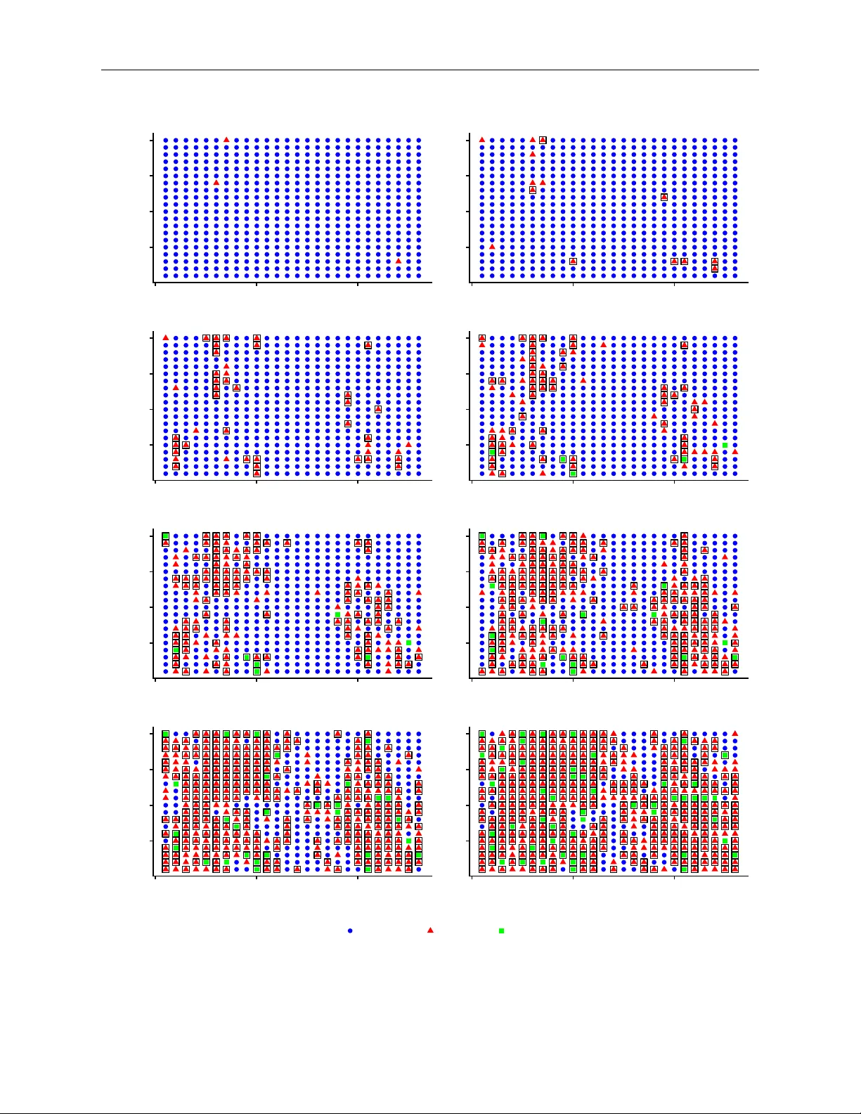
Hidden Mark o v Individual-lev el Mo dels of Infectious Disease T ransmission Dirk Dou wes-Sc h ultz 1 ∗ , Rob Deardon 1 , 2 and Alexandra M. Sc hmidt 3 1 Dep artment of Mathematics and Statistics, University of Calgary, Canada 2 F aculty of V eterinary Me dicine, University of Calgary, Canada 3 Dep artment of Epidemiolo gy, Biostatistics and Oc cup ational He alth, McGil l University, Canada F ebruary 17, 2026 Abstract Individual-lev el epidemic models are increasingly b eing used to help understand the transmission dynamics of v arious infectious diseases. Ho wev er, ﬁtting suc h mo dels to individual-lev el epidemic data is challenging, as we often only kno w when an individual’s disease status was detected (e.g., when they show ed symptoms) and not when they were infected or remov ed. W e prop ose an autoregressiv e coupled hidden Marko v mo del to infer unkno wn infection and remo v al times, as well as other mo del parameters, from a single observ ed detection time for each detected individual. Unlik e more traditional data augmentation metho ds used in epidemic mo delling, we do not assume that this detection time corresp onds to infection or remov al or that infected individuals must at some p oin t b e detected. Ba yesian coupled hidden Mark ov mo dels hav e b een used previously for individual-level epidemic data. How ever, these approac hes assumed eac h individual was contin uously tested and that the tests were indep enden t. In practice, individuals are often only tested un til their ﬁrst p ositiv e test, and even if they are con tinuously tested, only the initial detection times ma y b e rep orted. In addition, m ultiple tests on the same individual may not be indep enden t. W e accommo date these scenarios b y assuming that the probability of detecting the disease can dep end on past ∗ Corr esp onding author : Dirk Douw es-Sch ultz, Departmen t of Mathematics and Statistics, Uni- v ersity of Calgary , 2500 Univ ersity Driv e NW, Calgary , AB, Canada, T2N 1N4. E-mail : dirk.douwesschultz@ucalgary.ca . 1 2 Dou wes-Sc h ultz et al. observ ations, whic h allows us to ﬁt a muc h wider range of practical applications. W e illustrate the ﬂexibilit y of our approac h b y ﬁtting t wo examples: an experiment on the spread of tomato sp ot wilt virus in p epper plan ts and an outbreak of norovirus among n urses in a hospital. Key w ords : Ba yesian inference; Infectious disease modelling; Coupled hidden Mark ov mo del; Mark ov c hain Monte Carlo metho ds; Data augmentation; Stochastic epidemic mo del. 1 In tro duction Epidemiologists are often in terested in questions related to the transmission of an infectious disease at the individual level. F or example, whether susceptibility diﬀers b y individual-lev el c haracteristics such as age (Cohen et al., 1997; Davies et al., 2020), or ho w far an infected individual could realistically spread the disease (Hu et al., 2021; L ich temberg et al., 2022). Individual-lev el models (ILMs) of infectious disease transmission (Deardon et al., 2010) can b e v aluable tools for helping answer these t yp es of questions (V ynnyc ky and White, 2010). These approaches mo del eac h individual in the population mo ving through diﬀeren t disease states, such as susceptible, infectious, and remo v ed (W ard et al., 2025). T ransitions b et ween states can o ccur in contin uous (Almutiry et al., 2021) or discrete (W arriyar et al., 2020) time. W e will fo cus on discrete time. F or discrete-time mo dels, the probabilit y of infection at each time step may dep end on the num b er of infectious individuals in the p opulation, their distance from the susceptible individual, and the inheren t susceptibility or infectivity of individuals, whic h may v ary with co v ariates (Keeling et al., 2001; Mahsin et al., 2022). Therefore, these mo dels can describ e a wide range of complex mixing patterns. Ho wev er, a s igniﬁcant c hallenge with ﬁtting ILMs to individual-lev el epidemic data is that we usually only kno w when an individual w as detected (e.g, show ed symptoms), not when they were infected or remo ved (T ouloupou et al., 2020). F or example, in Section 4.2, w e lo ok at an experiment on the spread of tomato sp otted wilt virus (TSWV) in p epp er plan ts, which w as describ ed in Hughes et al. (1997) and analyzed using ILMs by Almutiry et al. (2021). The exp erimen ters only monitored a plant un til symptoms of TSWV app eared, so that the data consists of a single detection time for each detected plant (corresp onding to observ ed symptom onset). Since symptoms of TSWV take 2-4 weeks to app ear in a plant, plan ts w ere likely infected b efore they w ere detected. F urthermore, signs of TSWV can b e diﬃcult to sp ot in a plant; therefore, it is p ossible that the exp erimen ters never detected some infected plan ts. In this example, w e do not know the infection or remov al times or ev en ho w man y plan ts w ere infected, whic h mak es inference challenging. The most p opular w a y to account for uncertain infection and remov al times in epidemic 3 Dou wes-Sc h ultz et al. mo delling is to treat them as unkno wn parameters of the mo del within a Bay esian framework, whic h is kno wn as data augmentation (D A) (O’Neill, 2002; O’Neill and Kypraios, 2019). Most DA metho ds assume that infection times are unkno wn and remo v al times are known (O’Neill and Rob erts, 1999; Deardon et al., 2010; O’Neill and Kypraios, 2019), or that infection times are kno wn and remov al times are unkno wn (Bu et al., 2022). How ev er, in man y applications, we do not observe when individuals were remov ed or infected (Neal and Rob erts, 2004; P okharel and Deardon, 2022). In suc h cases, a susceptible-infectious-notiﬁed- remo ved (SINR) model (Jew ell et al., 2009) can b e used to estimate unkno wn infection and remo v al times using observed notiﬁcation (detection) times (Alm utiry et al., 2021). In an SINR mo del, all infectious individuals m ust en ter the notiﬁed state b efore transitioning to the remo ved state. That is, these mo dels assume that all infectious individuals m ust b e detected b efore remo v al. Ho wev er, infectious individuals could reco v er without b eing detected if, for example, they sho w mild or no symptoms and testing is based on the app earance of symptoms (Mullis et al., 2009). In addition, studies that use SINR mo dels ha v e made m uc h stronger assumptions. F or example, Jewell et al. (2009) assumed that the notiﬁcation and remo v al times were kno wn. Almutiry et al. (2021) did not require the remov al times to b e kno wn. Ho wev er, they assumed that only those who sho w ed symptoms w ere infected. It is p ossible for individuals who did not sho w symptoms to hav e b een infected, if they had asymptomatic infections, hard to sp ot symptoms, or w ere infected late in the study and had not y et developed symptoms (Jew ell et al., 2009). The assumption that no undetected individuals were infected during the observ ation p erio d is common when using many existing D A metho ds (Britton and O’Neill, 2002). This is b ecause, if there are undetected infections, traditionally complex reversible jump Marko v chain Monte Carlo (MCMC) steps m ust b e used to add and remov e infection times (O’Neill and Rob erts, 1999; Jew ell et al., 2009). T aking a very diﬀeren t approac h, T ouloup ou et al. (2020) prop osed using a coupled hidden Mark ov mo del (Pohle et al., 2021) to account for unknown infection and remov al times for discrete-time ILMs. They ﬁrst assumed that the epidemiological states of the individuals (e.g., susceptible, infectious, and remov ed) follo wed a series of coupled hidden Mark ov chains. By coupled, w e mean that the transition probabilities of an individual c hain, lik e the probabilit y of going from susceptible to infectious, could dep end on whether other individuals w ere in the infectious state. Then they generated the detection times conditional on the hidden states using an indep enden t Bernoulli observ ation model. There are man y imp ortan t adv an tages of this approac h ov er the more traditional D A metho ds describ ed in the previous paragraph. Firstly , unlike most of those metho ds, their mo del do es not assume that any of the detection times corresp ond to infection or remov al times. In addition, unlik e the SINR approach of Alm utiry et al. (2021), infectious individuals do not ha ve to b e detected 4 Dou wes-Sc h ultz et al. Figure 1: Shows the diﬀerence b et ween contin uous testing, assumed in T ouloup ou et al. (2020), and testing only up to the ﬁrst detection, whic h is more common in epidemiological studies. b efore remo v al, and undetected individuals (e.g., those who did not show symptoms) may ha ve b een infected during the study . Finally , all hidden state indicators for an individual can b e sampled directly from their full conditional distribution using the individual forward ﬁltering bac kward sampling (iFFBS) algorithm (T ouloup ou et al., 2020). This means that there is no need to use complex reversible jump MCMC steps to add or remov e infection times. Ho wev er, T ouloup ou et al. (2020) assumed that eac h individual w as contin uously tested for the disease (see Figure 1) and that the tests w ere indep enden t. In epidemiological stud- ies, individuals are often only tested un til they are ﬁrst detected, like in the TSWV example describ ed ab o ve, or the time of ﬁrst detection may b e the only a v ailable information (Sto c k- dale et al., 2017; Mizumoto and Cho well, 2020; Alm utiry et al., 2021). In addition, tests on the same individual ma y not b e independent. T o address the ab o ve limitations, w e extend the approach of T ouloupou et al. (2020) b y letting the probability of detecting the disease depend on past observ ations. This allo ws us to establish a stopping rule for the testing or reporting based on when an individual is ﬁrst detected. The resulting hidden Mark ov model is v ery general. It only requires a single detection time (e.g., corresp onding to symptom onset) for each detected individual. A dditionally , it do es not assume this detection time corresponds to infection or remov al, and do es not require infectious individuals to b e detected at an y p oin t. W e also show ho w more traditional DA metho ds can b e incorp orated into our framew ork, such as those assuming kno wn remov al (O’Neill and Rob erts, 1999) or infection (Bu et al., 2022) times. This allo ws these metho ds to b e ﬁt without the use of reversible jump MCMC steps. Also, since w e ﬁt all mo dels under a uniﬁed approac h, comparing them using the widely applicable information criterion (W AIC) (Gelman et al., 2014) is straigh tforw ard. This provides a data-driv en pro cedure to help c ho ose b et ween diﬀeren t DA metho ds (represented by separate observ ation mo dels), which has not b een considered in the literature to the b est of our kno wledge. The remainder of this pap er is organized as follows. Section 2 in tro duces the prop osed 5 Dou wes-Sc h ultz et al. hidden Marko v mo del for outbreak inv estigations in which there is only a single detection time for eac h detected individual. Section 3 discusses our Ba yesian inferen tial pro cedure, whic h makes use of the computationally eﬃcient iFFBS algorithm of T ouloup ou et al. (2020). In Section 4, we ﬁt our prop osed model to t wo examples: an outbreak of norovirus in a hospital and an exp eriment on the spread of tomato sp otted wilt virus in pepp er plan ts. W e also compare our approac h to several p opular alternatives from the literature, such as mo dels that assume kno wn infection or remov al times or that no undetected individuals w ere infected. W e close with a discussion in Section 5. 2 Hidden Mark o v Individual Lev el Mo delling F ramework Assume w e hav e a p opulation of i = 1 , . . . , N individuals who are observ ed across t = 1 , . . . , T time p eriods. Individual-level epidemic data usually takes the form of a collection of detection times for eac h individual. Let y it = 1 if individual i was detected as having the disease during time t (e.g., show ed symptoms), and 0 otherwise. W e fo cus on the case where there is at most a single detection time for each individual; see Section 2.1. This means that, for the detected individuals, y it will b e equal to 0 until their single detection time, then it will b e one, and then zero again until the end of the study; see the bottom graph of Figure 2. Finally , let S it b e an indicator for the true epidemiological state of the individual, where S it =        1 , if individual i w as susceptible during time t , 2 , if individual i w as infectious, 3 , if individual i w as remo ved. The detection times y it are observ ed, while the epidemiological states S it , which are of primary interest, are laten t, unobserv able quan tities. Therefore, we use a coupled hidden Mark ov mo del (P ohle et al., 2021) to infer the parameters of an SIR ILM from the observed detection times. This inv olves ﬁrst sp ecifying an observ ation mo del that describ es ho w the detection times are generated conditional on the disease states. Then we sp ecify a Mark ov mo del describing ho w the disease states ev olv e o ver time. 2.1 A general autoregressiv e observ ation pro cess T ouloup ou et al. (2020) considered a con tinuous testing observ ation mo del, whic h strongly implies that there should b e m ultiple detection times for at least some of the detected individuals; see Section 4.2. Ho wev er, it is m uch more common with individual-lev el outbreak data to ha ve only a single detection time for each detected individual (e.g., corresp onding to 6 Dou wes-Sc h ultz et al. symptom onset) (Sto c kdale et al., 2017; Kypraios et al., 2017; O’Neill and Kypraios, 2019; Sto c kdale et al., 2021; Almutiry et al., 2021). If there is only a single detection time per detected individual, then either individuals w ere only tested un til they were ﬁrst detected (see Figure 1), which is common in epidemiological studies (Mizumoto and Chow ell, 2020; Alm utiry et al., 2021), or individuals were contin uously tested and only the initial detection times were rep orted b y in v estigators. I n this section, we show that b oth of these scenarios lead to the same observ ation model. Firstly , we will assume that individuals are only tested for the disease un til they are ﬁrst detected. F or example, in the TSWV exp erimen t analyzed in Section 4.2, plan ts were only c heck ed for symptoms until they ﬁrst app eared (Hughes et al., 1997). The tests could b e lab oratory-based (T ouloup ou et al., 2020); visual and based on the app earance of symptoms (Alm utiry et al., 2021); or some combination of the t wo (Mizumoto and Cho well, 2020). In general, w e view a test as an y pro cedure, suc h as c hecking for symptoms, that has a non-zero probabilit y of detecting the disease if it is present. W e will also assume that there are no false p ositiv es, as otherwise identiﬁabilit y may be challenging with only one detection time a v ailable for each detected individual. If individuals are only tested until they ﬁrst test p ositiv e, the probability that an in- fectious individual is detected will b e giv en by the sensitivit y of the test, θ > 0 , until the individual is ﬁrst detected, and then it will b e 0, as the testing stops (if an individual is not tested, they will not b e detected). Therefore, w e sp ecify the observ ation model as y it | S it , y i 0 , . . . , y i ( t − 1) ∼      0 , if S it = 1 or 3 (susceptible or remo ved) Bern ( θ I [ y i 0 , . . . , y i ( t − 1) = 0]) , if S it = 2 (infectious) , (1) where we assume y i 0 = 0 , that no individuals were detected b efore the study started. In (1), I [ y i 0 , . . . , y i ( t − 1) = 0] is an indicator function whic h will b e 1 if individual i w as not detected previously and 0 if individual i was detected previously . Figure 2 shows a diagram of the mo del for a single detected individual. If there is only a single detection time for each detected individual, it could also b e that individuals were contin uously tested, but only the initial detection times w ere rep orted. F or ex ample, outbreak in vestigations often only rep ort the symptom onset time for each detected individual (Thompson and F o ege, 1968; Cáceres et al., 1998). If the decision to rep ort a test only dep ends on whether the individual w as previously detected, then (1) is still an appropriate observ ation mo del. T o see this, we can ﬁrst shift p erspective from the in vestigators to the mo deler (or an y outside observer) and assume y it represen ts whether the mo deler detects the disease in an individual. Then the probabilit y that the mo deler detects 7 Dou wes-Sc h ultz et al. Susceptible Inf ectious Re moved p 12,it 1/m Disease State θ 0 Prob . of Detection ● ● ● ● ● ● ● ● ● ● ● ● ● ● ● ● ● ● ● ● ● ● ● ● ● ● ● ● ● ● ● ● ● ● ● ● 0 1 Detected Figure 2: Sho ws a diagram of the prop osed hidden Mark ov individual-lev el mo del (HMM- ILM) for a single hypothetical detected individual. The b ottom graph shows the observ ations y it . the disease will b e θ un til the individual is ﬁrst detected, and then it will b e 0, since if a test is not rep orted, the mo deler will not detect the disease. Finally , w e note that the testing do es not necessarily ha ve to b e indep enden t ov er time as in T ouloup ou et al. (2020). F or example, supp ose that the test results of infectious individuals follo w a ﬁrst-order Mark ov chain, so that the probabilit y of testing p ositiv e is θ if the individual previously tested negativ e and θ 1 if the individual previously tested p ositiv e, with θ 1 > θ . Since individuals are only tested un til they ﬁrst test p ositiv e, all test results up to the detection time are negativ e, whic h means (1) still holds. 2.2 The hidden underlying SIR ILM W e assume that the disease state of individual i , S it , follo ws a three-state nonhomogeneous Mark ov chain. In order to accoun t for disease spread b et w een individuals, w e condition the transition matrix on S ( − i )( t − 1) = ( S 1( t − 1) , . . . , S ( i − 1)( t − 1) , S ( i +1)( t − 1) , . . . , S N ( t − 1) ) T , the vector of disease states for all individuals excluding individual i at time t − 1 . W e prop ose the 8 Dou wes-Sc h ultz et al. follo wing conditional transition matrix for the Mark ov chain, for t = 1 , . . . , T , Γ( S it | S ( − i )( t − 1) ) =       State S it =1 (sus.) S it =2 (inf.) S it =3 (rem.) S i ( t − 1) =1 (sus.) 1 − p 12 ,it p 12 ,it 0 S i ( t − 1) =2 (inf.) 0 1 − 1 m 1 m S i ( t − 1) =3 (rem.) 0 0 1       , (2) where Γ( S it | S ( − i )( t − 1) ) lk = P ( S it = k | S i ( t − 1) = l , S ( − i )( t − 1) ) and m is the a verage duration of the infectious p eriod, whic h w e will discuss more b elo w. In (2), p 12 ,it represen ts the probability that individual i is infected in the interv al [ t − 1 , t ) if they are susceptible at time t − 1 . W e will assume individual i primarily makes con tacts within a neighborho o d N E ( i ) . Let β j → i,t b e the probability of an infectious con tact b et w een individuals i and j ∈ N E ( i ) in the interv al [ t − 1 , t ) . Also, supp ose there is a small constant risk α of an individual b eing infected b y someone outside their neighborho o d (p oten tially outside the p opulation) or a bac kground reserv oir. Then, assuming all contacts are independent, we ha ve p 12 ,it = 1 − (1 − α ) Y j ∈ N E ( i ) (1 − β j → i,t ) I [ S j ( t − 1) =2] ≈ 1 − exp   − α − X j ∈ N E ( i ) β j → i,t I [ S j ( t − 1) = 2]   , (3) whic h follows the classic Reed-F rost formulation of a discrete-time SIR mo del (V ynn ycky and White, 2010; Deardon et al., 2010). Note that the approximation (3) holds only when β j → i,t is small for all j ∈ N E ( i ) , which may not b e appropriate if some individuals in the p opulation are closely connected. Therefore, w e more generally interpret β j → i,t > 0 as the eﬀect of disease spread from individual j to individual i in the contin uous time interv al [ t − 1 , t ) , and we generally do not restrict it to be less than 1. Deardon et al. (2010) proposed a very ﬂexible form for the eﬀects of disease spread, β j → i,t = S i T j K ij , where S i > 0 is a susceptibility function for susceptible individual i , T j > 0 is a transmissibility function for infectiv e j , and K ij > 0 is an infection kernel represen ting some contact measure b et ween i and j (e.g., distance). This form has b een extended in a m yriad of wa ys, for example, to allow for geographically v arying parameters (Mahsin et al., 2022) and to account for co v ariate measurement error (Amiri et al., 2024). F or ease of exp osition, and since w e mainly fo cus on the observ ation mo del, w e assume a more generic 9 Dou wes-Sc h ultz et al. sp eciﬁcation for the eﬀect of disease spread betw een individuals, β j → i,t = g ( β , x ij t ) , (4) where g ( · ) is a positive-v alued function, β is a v ector of unknown parameters, and x ij t is a v ector of co v ariates. F or example, x ij t could include the distance b et ween individuals i and j (Almutiry et al., 2021), the age of individual i or j (Beck er, 1989), or a temp oral indicator for the implementation of some control measure (Lek one and Finkenstädt, 2006). In (2), m > 1 represents the a v erage duration of the infectious p eriod. The adv an- tage of specifying the probabilit y of remo v al as 1 /m is that there is usually go o d prior information av ailable for m (Lapp e et al., 2023). How ev er, w e m ust b e cautious in in ter- preting m for some applications, as individuals can b e remov ed from the p opulation before they naturally reco ver from the disease; see Section 4.1. Finally , w e need to sp ecify an initial state distribution for the Marko v chain, that is, P ( S i 0 = k ) for i = 1 , . . . , N and k = 1 (susceptible) , 2 (infectious) , 3 (remo ved). This should b e done based on knowledge of the outbreak, for example, based on who w as lik ely the index case; see Section 4.1. F or our examples, w e will assume P ( S i 0 = 3) = 0 . W e will call the mo del deﬁned by Equations (1)-(4) the hidden Marko v individual-level mo del (HMM-ILM). Note that the HMM-ILM, unlik e most other epidemic models that emplo y DA metho ds (O’Neill and Kypraios, 2019), does not assume that the detection times correspond to either infection or remo v al times (see Figure 2). Additionally , from (1), infectious individuals can go undetected if they never test p ositiv e. This means the HMM-ILM can account for infections with mild or no symptoms, when the testing is based on the app earance of symptoms, or infections that o ccur near the end of the study and are not yet sho wing symptoms. That is, the HMM-ILM allo ws for b oth S → I → R and S → I transitions among undetected individuals. This is in contrast to the p opular existing D A metho ds describ ed in the in tro duction (O’Neill and Rob erts, 1999; Alm utiry et al., 2021), which, recall, do not allo w for S → I → R transitions among undetected individuals. F urthermore, while S → I transitions among undetected individuals (e.g., infections that o ccur near the end of the study) can be incorp orated in to traditional D A metho ds, complex rev ersible jump MCMC steps must then b e used to add or remov e infection times (Jewell et al., 2009). Therefore, many approaches assume no undetected individuals we re infected (O’Neill and Kypraios, 2019; Almutiry et al., 2021), meaning they cannot accoun t for late or asymptomatic infections. As w e sho w in the next section, another adv an tage of the HMM-ILM is a uniﬁed Bay esian inferential pro cedure where the hidden disease states for an individual are sampled directly from their full conditional distribution (T ouloup ou et al., 10 Dou wes-Sc h ultz et al. 2020); no complex rev ersib le jump MCMC steps or Metrop olis-Hastings prop osals for the states are required. 3 Inferen tial Pro cedure W e will ﬁrst show that the HMM-ILM is a hidden Marko v mo del. Let S t = ( S 1 t , . . . , S N t ) T b e the vector of epidemiological state indicators for all individuals at time t , y t = ( y 1 t , . . . , y N t ) T b e the v ector of observ ations for all individuals at time t , S = ( S 0 , . . . , S T ) T , and y = ( y 1 , . . . , y T ) T . The v ector S t follo ws a ﬁrst-order nonhomogeneous Mark ov c hain with state space { 1 , 2 , 3 } N and 3 N b y 3 N transition matrix Γ( S t ) . F rom Equation (2), an elemen t of Γ( S t ) is given b y , P ( S t = s t | S t − 1 = s t − 1 ) = N Y i =1 P ( S it = s it | S i ( t − 1) = s i ( t − 1) , S ( − i )( t − 1) = s ( − i )( t − 1) ) , where s t , s t − 1 ∈ { 1 , 2 , 3 } N . Therefore, rewriting the HMM-ILM mo del in terms of Γ( S t ) and p ( y t | y 0 , . . . , y t , S t ) = Q N i =1 p ( y it | y i 0 , . . . , y i ( t − 1) , S it ) , for t = 1 , . . . , T , and p ( S 0 ) = Q N i =1 p ( S i 0 ) sho ws that it is a hidden Mark ov mo del (see Chapter 10 of F rüh wirth-Schnatter (2006)). How ev er, the size of the transition matrix ( 3 N b y 3 N , where N is usually at least around 100) necessitates some changes to the standard inferential pro cedure of such mo dels (F rüh wirth-Sc hnatter, 2006), as we will no w discuss. Let v = ( θ , m , α, β ) T denote the v ector of all mo del parameters. The joint distribution of y and S giv en v is giv en b y p  y , S | v  = N Y i =1 p ( S i 0 ) T Y t =1 p  S it | S i ( t − 1) , S ( − i )( t − 1) , m, α, β  p  y it | y i 0 , . . . , y i ( t − 1) , S it , θ  . (5) F or the detected individuals, w e only observe the disease state indicator S it when they are detected, that is, only at the single p oin t where y it = 1 (then we must ha v e S it = 2 as we assume no false p ositiv es). F or the undetected individuals, we never observ e S it . It is also not p ossible to marginalize S from (5) to calculate L ( v ) = p ( y | v ) , the marginal likelihoo d function, as doing so would require matrix m ultiplication with Γ( S t ) (F rüh wirth-Schnatter, 2006). Therefore, w e treat the disease state indicators as unkno wn parameters of the model and sample S and v from their joint p osterior distribution, whic h is proportional to p ( S , v | y ) ∝ p ( y , S | v ) p ( v ) , (6) where p ( v ) is the prior distribution of v . Often, go o d prior information is av ailable for m (the 11 Dou wes-Sc h ultz et al. a verage duration of infectiousness) and/or θ (the probabilit y of initial detection). How ever, w e must b e cautious when interpreting these parameters for a giv en application, as discussed in more detail in the examples in Section 4. Regardless of the prior sp eciﬁcation, the join t p osterior distribution is not av ailable in closed form. Therefore, w e used a h ybrid Gibbs sampling algorithm with some steps of the slice sampling or Metrop olis-Hastings algorithms to sample from it. W e sampled m and θ using either univ ariate slice samplers (Neal, 2003) or adaptiv e random walk Metrop olis steps (Shab y and W ells, 2010), dep ending on the mixing. Since ( α, β ) T sho wed high p osterior correlations, w e jointly sampled it using automated factor slice sampling (Tibbits et al., 2014). It is straigh tforw ard to sample the state indicators one at a time from their full conditional distributions, p ( S it | S \ { S it } , y , v ) (Dou wes-Sc h ultz and Schmidt, 2022). How ever, we found that this mixed so slowly in our tw o examples and sim ulation studies that it is not usable. Join tly s ampling all of S from p ( S | y , v ) usually results in m uch faster mixing when ﬁtting HMMs (Chib, 1996). Ho w ever, this is not p ossible with the HMM-ILM, as it again requires matrix m ultiplication with Γ( S t ) . Therefore, we instead jointly sampled eac h individual’s disease state indicators, conditional on the disease state indicators for all other individuals, using the individual forw ard ﬁltering bac kward sampling (iFFBS) algorithm (T ouloup ou et al., 2020). More sp eciﬁcally , the iFFBS algorithm samples the vector of all state indicators for individual i , S i (0 : T ) = ( S i 0 , . . . , S iT ) T , from its full conditional distribution, p ( S i (0 : T ) | S ( − i )(0 : T ) , y , v ) = p ( S iT | S ( − i )(0 : T ) , y , v ) T − 1 Y t =0 p ( S it | S i ( t +1) , S ( − i )(0 : t +1) , y i (0 : t ) , v ) , (7) where S ( − i )(0 : T ) is S with S i (0 : T ) remo ved; see Supplemental Materials (SM) Section 1 for additional details. The hybrid Gibbs sampling algorithm w as implemented using the R pac k age NIMBLE (de V alpine et al., 2017). NIMBLE comes with built-in slice and automated factor slice samplers. W e implemented the iFFBS samplers using NIMBLE’s custom sampler fea- ture. All NIMBLE R co de and data for our motiv ating examples are a v ailable on GitHub https://github.com/Dirk- Douwes- Schultz/HMM_ILM_Code . In SM Section 2, we presen t a simulation study that sho ws our prop osed Gibbs sampler can recov er the true parameter v alues of an HMM-ILM, whic h is sp eciﬁed like in our TSWV example in Section 4.2. Finally , we note that to run the iFFBS algorithm, w e only require S it | S ( − i )( t − 1) to follow a ﬁrst-order Mark ov c hain and for y it to dep end only on S it and, p oten tially , on past observ a- tions (see Section 2.2.1 of Douw es-Sc hultz (2024) for a list of exact conditions). Therefore, it is v ery easy to mo dify the HMM-ILM. F or example, in Section 4.1, for comparison purp oses, 12 Dou wes-Sc h ultz et al. w e mo dify the observ ation pro cess (1) so that individuals are remov ed as so on as they are detected (O’Neill and Rob erts, 1999). Currently in the literature, even very similar ILMs are often ﬁt with v astly diﬀeren t MCMC algorithms (Jewell et al., 2009; Almutiry et al., 2021). A more uniﬁed inferential pro cedure, as we presen t here, could mak e these mo dels more easily adoptable for practitioners. 4 Applications T o ﬁt all mo dels discussed in this section, we ran our h ybrid Gibbs sampling algorithm for 200,000 iterations on three chains with an initial burn-in of 50,000 iterations. All c hains w ere started from random v alues in the parameter space to av oid conv ergence to lo cal mo des. Con- v ergence was c heck ed using the Gelman–Rubin statistic (all estimated parameters<1.05), the minim um eﬀective sample size (>1000), and b y visually examining the traceplots (Plummer et al., 2006). Unless indicated otherwise, no conv ergence issues were apparen t for any mo del discussed in this section. 4.1 Noro virus outbreak in a South Carolina hospital F or our ﬁrst example, we analyze a norovirus outbreak among 89 nurses in a South Carolina hospital in January 1996 (Cáceres et al., 1998). The observ ation p eriod for the outbreak in vestigation extended from the 5th to the 13th (t=1,. . . ,T=9). The data consists of 28 detection times, one for eac h detected n urse, whic h corresp ond to the da y the n urse ﬁrst rep orted sho wing symptoms in a survey administered by in vestigators. Figure 3 sho ws the epidemic curv e, that is, the n umber of new cases o ver time. The ﬁrst case was Nurse X on the ﬁfth. Nurse X w as though t to be the n urse who in tro duced the infection in to the w ard, as many of the early cases were traced back to her. The ward w as closed on the 12th, and after that, no new cases w ere rep orted. Kypraios et al. (2017) previously analyzed this data using a homogeneously mixing SIR mo del. How ever, they assumed that all the remo v al times in the interv al [1 , T ] had b een observ ed and were equal to the detection (i.e., symptom onset) times, which is a common assumption following the inﬂuen tial work of O’Neill and Roberts (1999). That is, they assumed that Nurse X was remov ed on the ﬁfth, that the four n urses detected on the seven th w ere remov ed that da y , and so on. Ho wev er, a snowstorm on the sev en th forced the nurses to sta y o vernigh t at the hospital, so they could not ha ve b een remo v ed that da y . Also, according to the inv estigation rep ort (Cáceres et al., 1998), many n urses con tinued to w ork after developing symptoms due to staﬀ shortages. A dditionally , since Kypraios et al. (2017) assumed they had observ ed all remo v al times in the in terv al [1 , T ] , they implicitly assumed 13 Dou wes-Sc h ultz et al. D a y (Ja n u a ry 1 9 9 6 ) C a se s (symp t o m o n se t ) 3 4 5 6 7 8 9 1 0 1 1 1 2 1 3 1 4 0 1 2 3 4 5 6 7 8 9 1 0 N u rse X Sn o w st o rm W a rd A C l o su re Figure 3: Cases in n urses by da y of symptom onset. Noro virus outbreak in a South Carolina hospital. none of the 61 undetected nurses had b een remo v ed during the observ ation p eriod. This is an often o verlooked issue with the framew ork of O’Neill and Rob erts (1999). Noro virus can frequen tly hav e mild or no symptoms (W ang et al., 2023), meaning it is not unreasonable to assume that at least some of the n urses were infected and reco vered without b eing detected. In contrast, the HMM-ILM allo ws individuals to b e remo ved ev en several da ys after detection, as illustrated in Figure 2. A dditionally , the HMM-ILM allows for S → I → R transitions among undetected individuals. Therefore, it ma y b e more suitable for this data. As w e hav e no individual-lev el information, w e used a simple homogeneous mixing mo del to describ e the eﬀects of disease spread b et ween the n urses, β j → i,t = β (1 − W t − 1 ) , (8) where W t is an indicator for whether the w ard w as closed that da y . That is, w e are assuming that if the w ard is closed, the nurses will not mix with each other. Given that there is no ob vious neighborho o d structure, w e let N E ( i ) = { j : j  = i } . During the outbreak in vestigation, the nurses w ere given surv eys in which they had to record the day they ﬁrst sho wed symptoms. Therefore, w e can interpret θ , from Equation (1), as the daily probability that an infectious nurse ﬁrst develops symptoms, m ultiplied b y the probability that the n urse notices (or remembers) symptoms given that they ha ve dev elop ed. Finally , for the initial state distributions, w e assumed that Nurse X had a 95% chance of b eing initially infected, as they lik ely introduced the infection into the ward (Cáceres et al., 1998). W e assumed that all other nurses had a low 1% c hance of b eing initially infected. 14 Dou wes-Sc h ultz et al. W e ﬁrst tried to ﬁt the HMM-ILM sp eciﬁed ab o ve using wide priors for all parameters. Ho wev er, with only 28 detection times, the p osteriors were very uninformative and the mo del had trouble conv erging. Therefore, we decided to use contact tracing information from the outbreak in vestigation (Cáceres et al., 1998) to specify informative priors for θ and m > 1 (the a verage length of the infectious p eriod). W e placed a Beta (40 , 40(6 / 4)) prior on θ to reﬂect an av erage of 1-2 days from exp osure to the ﬁrst rep orted app earance of symptoms, which w as found b y con tact tracing. F or m , an individual should b e infectious with noro virus for an a verage of 12 da ys without any interv en tion (Lapp e et al., 2023). Ho w ev er, it is unlik ely that infectious n urses would hav e work ed at the hospital for this en tire duration. F or example, the inv estigation rep ort talks ab out a nurse who ﬁrst show ed symptoms on the sev enth, sta yed o vernigh t due to the sno wstorm, w ork ed the next da y , and was not remo v ed un til the ninth. Therefore, we assume m is lik ely somewhere b et ween 1.5 (a verage time to ﬁrst rep orted symptoms) and 12 days, and w e placed a Gamma (2 , 2 / 5 . 75) prior on m − 1 . Finally , w e placed wide Unif (0 , 1) priors on β and α , from Equations (3) and (8). Figure 4 shows the prior and p osterior distributions of θ , m , α , and β . The prior and p osterior distributions of m and, esp ecially , θ are very similar, indicating that there is not a lot of information ab out these parameters in the data. In contrast, the data is m uch more informativ e ab out α and β . F rom the p osteriors, we estimate that there was a daily bac kground infection risk of 1.4% (0.08%, 4.8%) (p osterior median and 95% credible interv al), and that the probabilit y of an infectious con tact betw een a susceptible and infectious nurse w as 0.65% (0.2%, 1.5%) p er da y . This implies that an infectious nurse would pro duce an a verage of 2.61 (1, 7.04) secondary infections b efore recov ering in a completely susceptible p opulation, whic h is kno wn as the basic repro duction n umber R 0 = ( N − 1) β m (V ynnyc ky and White, 2010). The background infection risk could b e attributed to the 10 patients wh o w ere infected on the ward during the observ ation p erio d and are not typically included in the mo del (Britton and O’Neill, 2002; Kypraios et al., 2017). It ma y also represen t infections that are not w ell explained by the assumptions of the model, suc h as homogeneous mixing. W e can estimate the num b er of undetected nurses remov ed during the observ ation perio d b y lo oking at the p osterior median and 95% credible interv al of P 89 i =29 I [ S iT = 3] , which is 9 (1, 31) (w e let nurses 29-89 b e the undetected ones). Therefore, it is likely that at least a few n urses w ere infected and reco vered without b eing detected, p ossibly because they show ed no symptoms or did not complete the form accurately . This casts some doubt on the assumption made by Kypraios et al. (2017) that none of the undetected n urses were remov ed. How ev er, the credible interv al, while not including 0, is still very wide with only 28 detection times. Finally , w e can better understand ho w the outbreak evolv ed ov er time b y examining the p osterior probabilit y that a nurse w as in eac h epidemiological state during each day . W e 15 Dou wes-Sc h ultz et al. 0 2 4 6 8 0.2 0.3 0.4 0.5 0.6 P oster ior Prior Density of θ 0.00 0.05 0.10 0.15 0 1 5 10 15 20 25 P oster ior Prior Density of m 0 10 20 30 0.000 0.025 0.050 0.075 0.100 P oster ior Prior Density of α 0 50 100 150 0.00 0.01 0.02 P oster ior Prior Density of β Figure 4: P osterior and prior distributions of θ , m , α , and β from ﬁtting the HMM-ILM to the norovirus outbreak data. do this for one of the 4 n urses detected on the sev enth in SM Figure 5. F rom the ﬁgure, this nurse w as lik ely infected on the ﬁfth or sixth and not remo ved un til at least the nin th or ten th, which corresponds to the description of one of the n urses detected on the sev enth giv en in the in vestigation rep ort (as discussed ab o ve). This again casts some doubt on the assumption made in Kypraios et al. (2017) that this n urse w as remo ved on the seven th and w ould not ha ve b een able to infect an yone else on subsequen t da ys. Examining plots of the other n urses sho w ed a similar pattern of at least 2-4 days b et w een detection and remov al. W e can incorp orate kno wn remo v al times by mo difying the observ ation pro cess (1), y it | S it , y i 0 , . . . , y i ( t − 1) ∼      0 , if S it = 1 or 2 (susceptible or infectious) Bern ( I [ y i 0 , . . . , y i ( t − 1) = 0]) , if S it = 3 (remo v ed) . (9) Note (9) assumes we hav e observ ed the remov al time of ev ery n urse remo v ed in the interv al [1 , T ] , and that the remov al times are equal to the detection (i.e, symptom onset) times, as in Kypraios et al. (2017) and O’Neill and Rob erts (1999) (see ab o v e for an indepth discussion of these assumptions). Figure 5 compares the p osterior distribution of R 0 b et w een the HMM- ILM describ ed in the previous paragraphs and an HMM-ILM where (1) is replaced by (9), whic h w e will refer to as the known remov al times (KR T) mo del. Assuming known remov al 16 Dou wes-Sc h ultz et al. Unknown remo val times Known remo val times CDC estimate 0.0 0.2 0.4 0.6 0.8 0 3 6 9 Density P osterior of R 0 Figure 5: Shows the p osterior distribution of R 0 for a mo del that assumes unkno wn remov al times, our HMM-ILM, and a mo del that assumes kno wn remo v al times, that is, that the remo v al times are equal to the detection (i.e., symptom onset) times as in Kypraios et al. (2017). The v ertical dotted line is dra wn at the median R 0 estimate from Steele et al. (2020). times, a nurse’s remov al time is equal to their rep orted symptom onset time, meaning we can interpret m as the av erage duration from exp osure to rep orted symptoms. Therefore, w e placed a Unif (1 , 3) prior on m for the KR T mo del based on the con tact tracing discussed ab o v e. W e k ept the other model sp eciﬁcations the same. F rom Figure 5, assuming known remo v al times results in a muc h smaller and more con- cen trated p osterior for R 0 . A CDC study of 7,094 noro virus outbreaks found a median R 0 estimate of 2.75 (interquartile range 2.38-3.65) (Steele et al., 2020), which is not w ell rep- resen ted b y the p osterior from the KR T mo del. The p osterior median and 95% credible in terv al of the intercept α was 3.28% (0.53%, 6.64%) for the KR T model, while, recall, it w as 1.4% (0.08%, 4.8%) for our HMM-ILM. A large in tercept lik e this may indicate mo del misp eciﬁcation, since it implies that many of the infections cannot b e explained b y mixing b et w een the nurses. The KR T mo del attributes a signiﬁcant p ortion of the infection risk to background reservoirs, while producing an unrealistically low estimate of the risk from b et w een-nurse mixing, as represen ted b y R 0 . The t wo mo dels can also be compared using the widely applicable information criterion (W AIC) (Gelman et al., 2014; Douw es-Sch ultz et al., 2025), see SM Section 3. The mo del with the smallest W AIC is considered to hav e the b est ﬁt, and as a rule of thum b, a diﬀerence 17 Dou wes-Sc h ultz et al. of 5 or more in the W AIC is considered signiﬁcan t (Reich and Ghosh, 2019). The HMM- ILM had a W AIC of 221, while the KR T mo del had a W AIC of 222.36. Since the diﬀerence in W AIC is less than 5, this comparison is inconclusive. In SM Section 4.2, we carry out a sensitivit y analysis in which w e ﬁt several alternativ e mo dels, including those without an in tercept or assuming the outbreak had ceased, and we w ere still unable to ﬁnd an y signiﬁcan t diﬀerences in the W AIC. This suggests that the sample size of only 28 detection times may b e to o small to distinguish b et ween diﬀerent epidemic mo dels using mo del comparison criteria. This is despite the fact that imp ortan t mo del results can b e very sensitive to assumptions ab out the observ ation pro cess, as shown in Figure 5. Therefore, caution should b e exercised when analyzing smaller outbreaks. If w e cannot compare mo dels using comparison criteria, w e ha ve to rely more heavily on our a priori assumptions about the outbreak, whic h can ha ve a large impact on the results. F or this example, even though the W AIC is inconclusiv e, w e would argue our HMM-ILM more closely matc hes the description of the outbreak giv en in Cáceres et al. (1998) compared with the KR T mo del, and it also pro duces more realistic estimates, as discussed ab o v e. Note that small sample sizes are common when ﬁtting ILMs to incomplete epidemic data (O’Neill and Rob erts, 1999; Britton and O’Neill, 2002; Stockdale et al., 2017, 2021) (all with 40 or few er detection times). As we show in the next example, when the sample size is larger, 327 detection times, w e often do obtain signiﬁcan t diﬀerences in the W AIC. This is true even for mo dels that hav e similar sp eciﬁcations (like a linear versus a non-linear distance kernel). A dditionally , w e can use m uch wider priors for the mo del parameters and still obtain informative p osteriors. Therefore, this example needs to b e viewed in the context of its small sample size. 4.2 Exp erimen t on the spread of tomato sp otted wilt virus in p epp er plan ts F or our second example, w e analyze an exp erimen t on the spread of tomato sp otted wilt virus (TSWV) in p epp er plants, whic h was describ ed in Hughes et al. (1997). In this exp erimen t, they had N = 520 p epper plan ts planted in 26 ro ws of 20 plan ts eac h. Plants w ere c heck ed for symptoms of TSWV ev ery 2 weeks for 14 weeks ( t = 1 , . . . , T = 7 ). The exp erimen ters stopp ed monitoring a plant after it ﬁrst sho wed symptoms, so that the data consist of a single detection time for eac h detected plant (corresp onding to observed symptom onset). The detection times are plotted on a spatial grid in Figure 6. It is not clear ho w or where the infection w as in tro duced in the exp erimen t. The ﬁrst plant was detected at time t = 2 , and 327/520 plants had been detected b y the end of the observ ation perio d. Man y previous attempts to analyze this data ha v e assumed that the infection times are kno wn and equal to the detection times (Pokharel and Deardon, 2014, 2016; W arriyar et al., 2020; Bilo deau et al., 2024). How ev er, it takes 2-4 weeks for symptoms of TSWV to appear 18 Dou wes-Sc h ultz et al. 5 3 0 0 0 0 0 0 7 0 0 5 7 5 0 5 0 0 7 7 0 6 7 7 0 7 4 5 0 0 0 7 0 5 7 5 0 7 0 0 0 0 0 0 4 5 0 4 5 6 0 0 6 5 5 7 0 0 5 5 4 5 0 6 0 0 0 0 0 6 6 6 6 5 0 0 7 0 7 0 0 0 2 0 5 3 4 6 0 6 4 4 5 0 7 7 0 7 7 6 0 0 0 0 7 7 0 0 0 0 7 4 3 6 6 7 7 7 5 0 0 6 0 0 0 6 5 0 4 0 6 7 0 0 0 0 7 4 4 4 5 7 0 7 0 0 0 5 0 0 0 6 6 0 5 0 6 0 0 6 0 7 7 0 6 4 5 7 0 0 0 0 7 6 0 0 4 6 6 0 5 0 7 7 6 6 0 7 7 6 0 6 0 7 0 7 0 0 6 6 6 0 4 6 7 0 0 0 7 6 0 6 0 7 4 5 6 5 0 6 0 4 7 6 7 6 3 6 6 6 6 6 0 7 6 6 6 7 7 0 7 6 6 4 0 5 7 0 7 7 6 6 6 0 6 4 7 0 0 7 0 0 0 7 0 5 7 6 7 3 0 7 7 0 0 6 0 6 6 7 4 4 6 4 0 0 0 0 0 7 0 6 7 4 7 3 0 5 7 0 4 6 0 6 3 0 5 5 6 0 0 0 0 0 0 5 0 0 0 4 7 3 7 6 5 0 0 6 7 0 0 0 6 4 6 6 6 0 0 0 0 7 0 0 4 3 4 6 6 7 0 7 7 0 4 0 0 0 7 6 7 4 0 6 6 6 5 0 6 0 0 4 6 6 0 6 0 7 7 0 7 0 6 6 5 4 6 7 0 0 0 0 0 7 7 0 7 4 6 0 0 7 4 7 6 7 0 0 5 3 5 7 7 5 5 6 0 0 7 7 7 0 0 4 0 0 0 5 7 4 7 6 0 5 4 4 6 3 6 7 7 0 7 7 7 0 4 6 6 4 4 6 0 6 7 7 7 6 0 4 3 4 6 4 7 7 7 0 0 6 0 0 7 0 0 7 5 6 7 7 7 5 7 6 5 6 6 4 4 0 7 7 6 0 6 5 6 0 6 0 7 4 4 6 5 6 5 7 0 0 7 6 4 7 6 6 7 0 6 0 2.5 5.0 7.5 10.0 1 10 20 26 x (meters) y (meters) 0 30 60 90 1 2 3 4 5 6 7 t Cases (symptom onset) Figure 6: The left plot shows the detection time of each detected plant from the exp erimen t in Hughes et al. (1997). A b ox is dra wn around the ﬁrst plant detected at time t = 2 . A 0 corresp onds to the plant never b eing detected. The right plot sho ws the epidemic curve. in a plan t (Brust, 2024), meaning plants were lik ely infected b efore they w ere detected. Alm utiry et al. (2021) analyzed this data using an SINR mo del (see the introduction) and estimated the unkno wn infection and remo v al times of all 327 detected plants. Ho wev er, to a void the use of computationally in tensiv e reversal jump MCMC steps (Jew ell et al., 2009), they assumed that none of the 193 undetected plants w ere infected. Some of the undetected plan ts could ha v e b een infected near the end of the exp erimen t and w ould ha ve p erhaps sho wn symptoms if the observ ation p erio d had b een extended (it takes 2-4 weeks for symptoms to dev elop). Indeed, the epidemic curve, plotted in Figure 6, is at its p eak, indicating that we w ould likely see more cases if the exp erimen t had gone on longer. Also, some undetected plan ts could ha ve had asymptomatic infections or symptoms that were hard to spot (Mullis et al., 2009). In contrast, the HMM-ILM allows plan ts to b e detected after they ha ve b een infected; see Figure 2. F urthermore, the HMM-ILM allo ws for the possibility that undetected plan ts w ere infected and never show ed symptoms during the observ ation p eriod; see Equation (1). Therefore, an HMM-ILM may b e more suitable for this data. TSWV is transmitted from plan t to plant b y small insects called thrips (Mullis et al., 2009). It seems reasonable to assume that the thrips are more lik ely to mov e to closer plants compared to those farther a wa y . Therefore, w e used a second-order T aylor series appro ximation of the p o w er-law dis- tance kernel (Deardon et al., 2010) to describ e the eﬀect of disease spread b et ween plants 19 Dou wes-Sc h ultz et al. (see Equation (3)), β j → i,t = β j → i = β 0 β − d ij 1 ≈ β 0 d − a ij  1 − ln( d ij )( β 1 − a ) + . 5 ln( d ij ) 2 ( β 1 − a ) 2  , (10) where d ij is the distance (in meters) betw een plan ts i and j . In (10), β 0 > 0 represen ts the eﬀect of disease spread from plan ts one meter aw ay , while β 1 > 0 represen ts how fast the eﬀect of disease spread decays with the distance betw een the t wo plants. W e used a T aylor series appro ximation as it allows us to factor β 0 and β 1 from the sums P j ∈ N E ( i ) β j → i,t I [ S j ( t − 1) = 2] in Equation (3). This means w e do not need to up date these sums when up dating β 0 and β 1 in our MCMC algorithm, whic h sa v es a lot of computational time. Note that the T aylor series appro ximation is alwa ys p ositiv e. W e set a = 1 . 35 , whic h is a guess for β 1 , from W arriy ar et al. (2020). In SM Section 5.1, w e in v estigate some alternativ e distance k ernels, including linear kernels, β j → i = β 0 + β 1 d ij ; quadratic k ernels, β j → i = β 0 + β 1 d ij + β 2 d 2 ij (with p ositivit y constrain ts); and spline-based kernels. W e found the HMM-ILM with Equation (10) had the low est W AIC b y a signiﬁcant amount, so w e use this expansion throughout this section. W e also compared the T aylor appro ximation with the exact p ow er-law and found they had the same W AIC, meaning the T aylor series appro ximation do es not appear to negativ ely aﬀect the ﬁt. In this example, w e can interpret θ as the probability that symptoms develop in a plant m ultiplied b y the probabilit y that the experimenters notice symptoms giv en that they hav e dev elop ed. Since it is unclear ho w easy it w as to observe the symptoms—they can b e hard to sp ot (Mullis et al., 2009)—we used a wide prior for θ ∼ Unif (0 , 1) . W e also used a wide prior for m ∼ Unif(1,20), α ∼ Unif (0 , 1) , β 0 ∼ Unif (0 , 1) , and β 1 ∼ Unif (0 , 20) . As it is not known ho w the disease was in tro duced in the exp erimen t, w e assumed each plant had a lo w 1% c hance of b eing initially infected. Finally , concerning the neighborho o d set N E ( i ) , there is lik ely a maxim um distance w e w ould expect the thrips to b e able to tra vel within 2 w eeks. Therefore, we started with a second-order queen neighborho o d structure (all plan ts at most 2 plan ts aw ay , including on the diagonal) (Nguyen et al., 2025) and increased the neigh b orho od order b y one un til the W AIC decreased b y less than 5. The second-order neigh b orho od mo del had a W AIC of 1602.68, the third-order mo del had a W AIC of 1591.76, and the fourth-order mo del had a W AIC of 1587.32. Therefore, we let N E ( i ) include all plan ts at most three plan ts a wa y from plan t i (see SM Figure 7). The top graphs of Figure 7 sho w the prior and p osterior distributions of θ and m . The p osterior median and 95% credible interv al of θ is 0.53 (0.43, 0.65), meaning w e estimate that it to ok an infected plant 1.77 (1.08, 2.65) weeks to b e detected on a v erage. This corresp onds 20 Dou wes-Sc h ultz et al. 0 2 4 6 0.4 0.5 0.6 0.7 0.8 P oster ior Prior Density of θ 0.00 0.05 0.10 0.15 5 10 15 20 P oster ior Prior Density of m 0.0 0.1 0.2 0.3 0.4 0.5 0.5 1.0 2.0 3.0 Distance from inf ected plant (meters) Probability of Inf ection (within two weeks) Figure 7: The top graphs sho w the p osterior and prior d istributions of θ and m from ﬁtting our HMM-ILM to the TSWV exp erimen t. The b ottom graph shows the probabilit y that a susceptible plan t is infected (within t w o w eeks), given a single infectious plant as a function of the distance betw een the tw o plan ts (posterior median and 95% credible interv al). with the kno wn incubation p erio d (Brust, 2024). Although the p osterior of m is wide, there is a 95% c hance that the av erage duration of the infectious p erio d is at least 20 weeks. Plants are infected with TSWV until they die (Co op er and Meado ws, 2024), so a long infectious p eriod lik e this seems plausible. In our sim ulation study in SM Section 2, w e found that when the true v alue of m is greater than T , the p osterior is often wide as seen in Figure 7. In contrast, when the true v alue of m is less than T , the p osterior is usually muc h more concen trated around the true v alue. This suggests that when the av erage duration of the infectious p eriod is greater than the length of the observ ation p erio d , it can b e c hallenging to estimate m . The b ottom graph of Figure 7 sho ws the probability that a susceptible plan t is infected (within tw o weeks), given a single infectious plan t versus the distance b et w een the t wo plan ts. F or example, if a susceptible plant is half a meter from an infectious plant (the minim um distance in the exp erimen t), it would hav e a 39% (23%, 49%) chance of b eing infected within 21 Dou wes-Sc h ultz et al. 2.5 5.0 7.5 10.0 0 10 20 x (meters) y (meters) Known inf ection Likely inf ection Figure 8: The circles represen t plants that w ere detected during the experiment. The crosses represen t undetected plants whose p osterior probability of having b een infected dur- ing the exp erimen t, P ( S iT = 2 or 3 & S i 0 = 1 | y ) , is greater than .5. t wo w eeks. If the plant were 2 meters a wa y , it would ha ve only a 3% (2%, 4%) chance of b eing infected. Therefore, we can see from the ﬁgure that the probability of infection decays v ery rapidly with the distance from an infected plant. In particular, susceptible plants more than 1.5 meters a wa y from an infected plant are unlik ely to b e infected within 2 weeks, so the range of dispersal is fairly short. Note that the exact equation plotted, from Equations (3)+(10), is 1 − exp  − α − β 0 d − a ij  1 − ln( d ij )( β 1 − a ) + . 5 ln( d ij ) 2 ( β 1 − a ) 2   v ersus d ij . The p osterior probability that an undetected plant i was infected during the exp erimen t is given by P ( S iT = 2 or 3 & S i 0 = 1 | y ) ≈ 1 Q − M P Q q = M +1 I [ S [ q ] iT = 2 or 3 & S [ q ] i 0 = 1] , where the sup erscript [ q ] denotes a dra w from the p osterior distribution of the v ariable, Q is the total n umber of MCMC samples, and M is the size of the burn-in sample (w e remo v ed infections o ccurring b efore the exp erimen t (t=0) to make things easier to interpret, but the follo wing results are the same either wa y). Therefore, w e can iden tify undetected plants that were likely infected during the experiment b y ﬁnding undetected plan ts i for which P ( S iT = 2 or 3 & S i 0 = 1 | y ) > 0 . 5 . W e plot the lo cation of suc h plan ts in Figure 8 (denoted b y crosses). F rom the ﬁgure, we can see that many undetected plants in close proximit y to plan ts that sho w ed symptoms w ere lik ely infected during the experiment. These undetected 22 Dou wes-Sc h ultz et al. plan ts may hav e had asymptomatic infections or were in fected late in the exp erimen t and not yet showing symptoms. W e can estimate the total num b er of undetected plants infected during the exp erimen t by lo oking at the p osterior median and mean of P i : y it =0 ∀ t I [ S iT = 2 or 3 & S i 0 = 1 ] . W e ﬁnd this to b e 94 (58, 133). Therefore, ev en on the lo w end of our estimation, w e would exp ect 58 of the undetected plan ts to ha ve b een infected during the exp erimen t. This suggests that the analysis from Alm utiry et al. (2021), who assumed that none of the undetected plants were infected, w as based on o ver-simpliﬁed assumptions. F or comparison purposes, w e can incorporate the assumption that no undetected plan ts w ere infected, as in Alm utiry et al. (2021), by ﬁxing S it = 1 (susceptible) for all undetected plan ts i and t = 0 , . . . , 7 (see the beginning of the section for an in-depth discussion of this assumption). In this case, we only run the iFFBS algorithm for the 327 detected plan ts, as the rest of the state indicators are kno wn. W e can incorp orate kno wn infection times, like in Bilo deau et al. (2024) or W arriyar et al. (2020), by modifying the observ ation pro cess (1), y it | S it , y i 0 , . . . , y i ( t − 1) ∼      0 , if S it = 1 or 3 (susceptible or remo ved) Bern ( I [ y i 0 , . . . , y i ( t − 1) = 0]) , if S it = 2 (infectious) . (11) Note Equation (11) assumes we ha ve observ ed the infection time of every plan t infected in the interv al [1 , T ] , and that the infection times are equal to the detection times (i.e., when the plant ﬁrst show ed symptoms). This is equiv alen t to assuming θ = 1 in Equation (1), that is, that the disease was p erfectly detected. Finally , w e also wan t to consider the con tin uous testing mo del of T ouloup ou et al. (2020), since it could be naiv ely applied in an application lik e this (where we ha ve only a single detection time for eac h detected individual). T ouloup ou et al. (2020) assumed individuals k ept b eing tested for the disease ev en after they w ere ﬁrst detected, so that w e can replace (1) b y , y it | S it ∼      0 , if S it = 1 or 3 (susceptible or remo ved) Bern ( θ ) , if S it = 2 (infectious) . (12) Note that if individuals were contin uously tested, we would exp ect to see multiple detection times for at least some of the detected individuals. Having only a single detection time for eac h detected individual would b e very unlikely under this mo del. Figure 9 compares the probabilit y of infection v ersus distance and W AIC of (a) the prop osed HMM-ILM, (b) an HMM-ILM with (1) replaced by (12) (T ouloup ou et al., 2020), (c) an HMM-ILM with (1) replaced b y (11) (known infection times), and (d) an HMM-ILM ﬁxing S it = 1 for all undetected plan ts (no undetected plan ts infected). F or the comparison 23 Dou wes-Sc h ultz et al. 0.0 0.1 0.2 0.3 0.4 0.5 0.5 1.0 2.0 3.0 Distance from infected plant (meters) (a) HMM−ILM, W AIC = 1592 Probability of Infection (within tw o weeks) 0.0 0.1 0.2 0.3 0.4 0.5 0.5 1.0 2.0 3.0 Distance from infected plant (meters) (b) T ouloupou (2020), WAIC = 1724 Probability of Infection (within tw o weeks) 0.0 0.1 0.2 0.3 0.4 0.5 0.5 1.0 2.0 3.0 Distance from infected plant (meters) (c) Known inf ection times (equals detection times), WAIC = 1690 Probability of Infection (within tw o weeks) 0.0 0.1 0.2 0.3 0.4 0.5 0.5 1.0 2.0 3.0 Distance from infected plant (meters) (d) No undetected plants infected, W AIC = 1628 Probability of Infection (within tw o weeks) Figure 9: Shows the probability that a susceptible plan t is infected (within t wo w eeks) giv en a single infectious p lant as a function of the distance betw een the t wo plants, for four mo dels ﬁtted to the TSWV exp erimen t. Sho ws p osterior medians and 95% credible in terv als. mo dels, w e used the same priors and also k ept the other model sp eciﬁcations the same. As sho wn in the ﬁgure, the HMM-ILM has the lo west W AIC by a signiﬁcant amoun t (more than 5), meaning that it has the b est ﬁt to the data. In addition, assuming contin uous testing, kno wn infection times, or that no undetected plan ts were infected, all result in estimating a m uc h ﬂatter distance kernel. F or example, for a susceptible plant half a meter aw a y from an infectious plant, our HMM-ILM estimates an inf ection risk of 39% (23%, 49%), while the mo del assuming no undetected plants w ere infected estimates an infection risk of only 19% (12%, 27%), which is half as large. A p ossible explanation for this diﬀerence is that, from Figure 8, man y of the undetected plants that w ere likely infected w ere adjacent to plan ts with kno wn infections in the same row, half a meter a wa y . Therefore, if w e assume that none of those undetected plants were actually infected, we would exp ect to see a m uch smaller estimate of the eﬀect of disease spread b et ween close plan ts, as we observ e in Figure 9 (d). F or this example, w e w ould expect to see a large spatial eﬀect, as seen in the HMM-ILM in 24 Dou wes-Sc h ultz et al. Figure 9 (a), as TSWV is transmitted b y thrips that mo ve from plan t to plant (Mullis et al., 2009). T o help dig deep er into the diﬀerences b et w een the mo dels, we giv e the full set of p osterior distributions of each model from Figure 9 in SM Section 5.2. In terestingly , assuming no undetected plan ts were infected leads to a posterior for θ that is concentrated close to one. This makes sense intuitiv ely . If w e assume that no undetected plan ts w ere infected, then ev ery plant that w as infected must ha ve been detected. This then implies a high c hance of detecting the disease in a plant. How ev er, since it tak es 2-4 w eeks for symptoms to app ear in a plan t (Brust, 2024), it seems unlik ely that we w ould ha ve a probabilit y close to one for a plant to b e detected in the same time step it w as infected, as implied b y this mo del. Also in terestingly , assuming contin uous testing leads to a p osterior for m that is concen trated close to one. Again, this mak es sense intuitiv ely . If individuals were infectious for more than one time step, then a con tin uous testing mo del w ould heavily imply that we w ould observe m ultiple detection times for at least some detected individuals. Therefore, the only wa y to explain a single detection time for eac h detected individual is if m = 1 . Ho w ever, this seems unlik ely giv en plan ts are infectious with TSWV until death (Co oper and Meadows, 2024). 5 Discussion W e ha ve prop osed a hidden Mark ov mo del for analyzing individual-level outbreak data where w e hav e only a single detection time for each detected individual, which is v ery common in practice (Sto c kdale et al., 2017; Kypraios et al., 2017; O’Neill and Kypraios, 2019; Sto c k dale et al., 2021; Alm utiry et al., 2021). F or example, this detection time ma y correspond to when symptoms ﬁrst appeared in an individual, as in our examples, or it could represent when individuals ﬁrst tested p ositiv e on a lab oratory test (Mizumoto and Cho well, 2020). Unlike most other approac hes built around data augmen tation metho ds (O’Neill and Rob erts, 1999; O’Neill and Kypraios, 2019), w e do not assume the detection times corresp ond to infection or remo v al times. As w e show ed in our examples, imp ortan t mo del results, such as estimates of R 0 , can b e very sensitive to assumptions ab out whether the infection or remov al times are known. F or instance, in our norovirus example, assuming known remo v al times led to an unrealistically lo w estimate of betw een-nurse transmission. In our TSWV example, assuming kno wn infection times resulted in estimating a m uch ﬂatter distance k ernel and a w orse mo del ﬁt. In addition, an often ov erlo ok ed assumption of the p opular known remo v al times framew ork of O’Neill and Rob erts (1999) is that no infectious individuals can b e remov ed without b eing detected. This means these mo dels cannot accoun t for infections with mild or no symptoms, when testing is based on the app earance of symptoms, or remov als that are 25 Dou wes-Sc h ultz et al. not recorded for other reasons. In contrast, our HMM-ILM allows infectious individuals to reco ver b efore testing p ositiv e, and we can estimate the n umber of undetected remov als as sho wn in the norovirus example. Alm utiry et al. (2021) prop osed using an SINR mo del (Jewell et al., 2009) to estimate infection and remo v al times when b oth are unkno wn. How ever, their framework only esti- mates the infection and remov al times of the detected individuals (e.g., those who show ed symptoms) and assumes that none of the undetected individuals w ere infected. In contrast, our HMM-ILM allo ws infectious individuals to go u ndetected if they never test p ositiv e. This means, when testing is based on the app earance of symptoms, w e can account for undetected individuals who had asymptomatic infections or w ere just infected late in the study and not y et showing symptoms. F or the TSWV example, w e found that at least 58 of the undetected plan ts w ere likely infected during the exp erimen t, an asp ect the analysis of Almutiry et al. (2021) did not accoun t for. In addition, assuming no undetected plan ts w ere infected led to estimating a muc h ﬂatter distance kernel and a w orse mo del ﬁt. Some of the restrictive assumptions in A lmutiry et al. (2021) could b e relaxed using computationally in tensive re- v ersible jump MCMC steps (Jew ell et al., 2009). Ho wev er, these steps only add infection times, not remo v al times (they assume that remov al o ccurs sometime after the end of the observ ation p erio d). Therefore, this would only allow for S → I transitions among unde- tected individuals (e.g, late infections) and not S → I → R transitions (e.g, asymptomatic infections), whic h are allow ed b y the HMM-ILM. T ouloup ou et al. (2020) also analyzed individual-level outbreak data usin g coupled hidden Mark ov mo dels. Ho w ever, they assumed eac h individual w as contin uously tested for the disease. If individuals were con tin uously tested, then we would exp ect to observ e multiple detection times for at least some of the detected individuals. Ho wev er, in man y applications, suc h as in the examples considered here, we hav e only a single detection time for eac h detected individual (Sto c kdale et al., 2017, 2021; O’Neill and Kypraios, 2019). In the TSWV example, our HMM-ILM ﬁt signiﬁcantly b etter than the mo del of T ouloup ou et al. (2020) and was able to capture a muc h stronger spatial eﬀect. If w e ha ve only a single detection time for eac h detected individual, then either individuals stopp ed b eing tested after their ﬁrst p ositiv e test, as in the TSWV example (Hughes et al., 1997), or individuals were con tinuously tested and only the initial detection times w ere rep orted b y the inv estigators. Both scenarios should lead to the same observ ation mo del (1), as we justify in Section 2.1. Indeed, it seems a necessary condition for mo deling suc h data is that the probability of detection drops to 0 after the ﬁrst detection, as in Equation (1), or we w ould exp ect to observe m ultiple detection times for at least some of the detected individuals. W e sho wed that b y rewriting Equation (1), we can consider a wide range of observ ation 26 Dou wes-Sc h ultz et al. pro cesses: testing only up to the ﬁrst detection (1), con tinuous testing (12), kno wn remo v al times (9), and kno wn infection times (11). F uture w ork should consider further observ ation mo dels. F or instance, in the T ristan da Cunha cold example from Bec ker (1989), they observ ed the start and end of symptoms for eac h individual who sho wed symptoms. This could b e mo deled b y letting y it | S it = 2 follo w a Marko v c hain. W e could also consider a m ultiv ariate observ ation vector y it in cases where w e observe m ultiple even ts, such as death and the developmen t of diﬀerent kinds of symptoms (Neal and Rob erts, 2004). In our examples, we found that imp ortan t results (e.g., estimates of R 0 ) can b e very sensitiv e to assumptions ab out the observ ation pro cess, such as whether remo v al times are kno wn. As suc h, future w ork should carefully consider the c hoice of the observ ation mo del based on in vestigation rep orts and b y using model comparison criteria, suc h as the W AIC, as w e did here. There are some imp ortan t limitations of our w ork. W e only consider SIR compartmen- tal mo dels. The iFFBS algorithm, whic h is the cornerstone of our inferen tial procedure, only requires that S it | S ( − i )( t − 1) follo w a ﬁrst-order Marko v c hain (Douw es-Sc hultz, 2024). Therefore, extensions to more complex compartmental mo dels, such as susceptible-exp osed- infectious-remo ved (SEIR) mo dels (Bu et al., 2025), should be straigh tforward in theory . Ho wev er, SEIR mo dels can suﬀer from serious iden tiﬁability problems when only remov al times are observed (O’Neill and Kypraios, 2019). The observ ation process deﬁned in Equa- tion (1) provides less information ab out the parameters than knowing the remov al times (e.g., compare the widths of the p osteriors in Figure 5). Therefore, to ﬁt SEIR hidden Mark ov mo dels, additional data and diﬀeren t observ ation pro cesses w ould lik ely ha ve to b e consid- ered, and/or m uch more informativ e priors could b e used for some of the parameters. A p ossible solution could b e to use the kno wn infection times observ ation process (11), whic h, with the additional assumption that there were no undetected infections, is similar to the analysis in Bu et al. (2025) (the justiﬁcation b eing that when individuals transition from E → I they sho w symptoms). Ho wev er, this w ould not accoun t for asymptomatic infections. Another limitation is that we assume the test sensitivity , θ from Equation (1), is constan t. F or instance, in the TSWV example, we assume that the probability that an infectious plant dev elops observ able symptoms is the same for ev ery time step it is infected. Since it tak es 2-4 w eeks for the symptoms to develop, it would be more realistic to let θ b e 0 for the ﬁrst time step of infectiousness, an unknown quan tit y to b e estimated for time step 2, and then 0 again after time step 2. That is, if the plan t has not developed symptoms after a mon th or so, it likely will not develop them. This could b e accomplished by splitting up the infectious compartmen t in to sub-compartments. Finally , individuals often change their b eha vior dur- ing an epidemic in resp onse to others around them showing symptoms (W ard et al., 2023, 27 Dou wes-Sc h ultz et al. 2025) and to their own symptoms. This could b e incorp orated into the HMM-ILM by letting β j → i,t dep end on y i 0 , . . . , y i ( t − 1) and y j 0 , . . . , y j ( t − 1) . Note that the iFFBS algorithm allows for autoregression in the transition probabilities (Douw es-Sch ultz, 2024). W e will consider extensions suc h as this in future w ork. References Alm utiry , W., KV, V. W. and Deardon, R. (2021) Con tin uous time individual-level mo dels of infectious disease: P ac k age EpiILMCT. Journal of Statistic al Softwar e , 98 , 1–44. Amiri, L., T orabi, M. and Deardon, R. (2024) Spatial mo delling of infectious diseases with co v ariate measurement error. Journal of the R oyal Statistic al So ciety Series C: Applie d Statistics , 73 , 460–477. Bec ker, N. G. (1989) Analysis of Infe ctious Dise ase Data . Chapman and Hall/CR C. Bilo deau, B., Stringer, A. and T ang, Y. (2024) Sto c hastic con vergence rates and applica- tions of adaptive quadrature in Bay esian inference. Journal of the A meric an Statistic al Asso ciation , 119 , 690–700. Britton, T. and O’Neill, P . D. (2002) Ba yesian inference for sto c hastic epidemics in popula- tions with random social structure. Sc andinavian Journal of Statistics , 29 , 375–390. Brust, G. (2024) The curious case of the virus infected tomato fruit. V e getable and F ruit News , 15 , 3–4. Bu, F., Aiello, A. E., V olfovsky , A. and Xu, J. (2025) Sto c hastic EM algorithm for partially observ ed sto c hastic epidemics with individual heterogeneity . Biostatistics , 26 , kxae018. Bu, F., Aiello, A. E., Xu, J. and V olfovsky , A. (2022) Likelihoo d-based inference for partially observ ed epidemics on dynamic netw orks. Journal of the A meric an Statistic al Asso ciation , 117 , 510–526. Cáceres, V. M., Kim, D. K., Bresee, J. S., Horan, J., Noel, J. S., Ando, T., Steed, C. J., W eems, J. J., Monro e, S. S. and Gibson, J. J. (1998) A viral gastro en teritis outbreak asso ciated with p erson-to-person spread among hospital staﬀ. Infe ction Contr ol & Hospital Epidemiolo gy , 19 , 162–167. Chib, S. (1996) Calculating posterior distributions and mo dal estimates in Mark o v mixture mo dels. Journal of Ec onometrics , 75 , 79–97. 28 Dou wes-Sc h ultz et al. Cohen, S., Doyle, W. J., Sk oner, D. P ., Rabin, B. S. and Gwaltney , J. M. (1997) So cial ties and susceptibilit y to the common cold. JAMA , 277 , 1940–1944. Co oper, A. and Meado ws, I. (2024) T omato sp otted wilt virus on tomato and p epp er. T ech- nical report, NC State Extension Publications. Da vies, N. G., Klepac, P ., Liu, Y., Prem, K., Jit, M. and Eggo, R. M. (2020) Age-dep enden t eﬀects in the transmission and control of COVID-19 epidemics. Natur e Me dicine , 26 , 1205–1211. Deardon, R., Bro oks, S. P ., Grenfell, B. T., Keeling, M. J., Tildesley , M. J., Savill, N. J., Sha w, D. J. and W o olhouse, M. E. J. (2010) Inference for individual-lev el mo dels of infec- tious diseases in large p opulations. Statistic a Sinic a , 20 , 239. Dou wes-Sc h ultz, D. (2024) Couple d Markov switching mo dels for sp atio-temp or al infe ctious dise ase c ounts . Ph.D. thesis, McGill Universit y . URL: https://escholarship.mcgill. ca/concern/theses/6395wf20p . Dou wes-Sc h ultz, D. and Sc hmidt, A. M. (2022) Zero-state coupled Mark o v switching coun t mo dels for spatio-temp oral infectious disease spread. Journal of the R oyal Statistic al So ciety: Series C (Applie d Statistics) , 71 , 589–612. Dou wes-Sc h ultz, D., Sc hmidt, A. M., Shen, Y. and Buck eridge, D. L. (2025) A three-state coupled Marko v switching model for COVID-19 outbreaks across Queb ec based on hospital admissions. The Annals of Applie d Statistics , 19 , 371–396. F rüh wirth-Sc hnatter, S. (2006) Finite Mixtur e and Markov Switching Mo dels . Springer Series in Statistics. New Y ork: Springer-V erlag. Gelman, A., Hwang, J. and V ehtari, A. (2014) Understanding predictive information criteria for Ba y esian mo dels. Statistics and Computing , 24 , 997–1016. Hu, M., Lin, H., W ang, J., Xu, C., T atem, A. J., Meng, B., Zhang, X., Liu, Y., W ang, P ., W u, G. et al. (2021) Risk of coronavirus disease 2019 transmission in train passengers: an epidemiological and mo deling study . Clinic al Infe ctious Dise ases , 72 , 604–610. Hughes, G., McRob erts, N., Madden, L. V. and Nelson, S. C. (1997) V alidating mathematical mo dels of plan t-disease progress in space and time. Mathematic al Me dicine and Biolo gy: A Journal of the IMA , 14 , 85–112. Jew ell, C. P ., Kypraios, T., Neal, P . and Rob erts, G. O. (2009) Bay esian analysis for emerging infectious diseases. Bayesian A nalysis , 4 , 465–496. 29 Dou wes-Sc h ultz et al. Keeling, M. J., W o olhouse, M. E., Sha w, D. J., Matthews, L., Chase-T opping, M., Ha ydon, D. T., Cornell, S. J., Kapp ey , J., Wilesmith, J. and Grenfell, B. T. (2001) Dynamics of the 2001 UK fo ot and mouth epidemic: sto c hastic disp ersal in a heterogeneous landscap e. Scienc e , 294 , 813–817. Kypraios, T., Neal, P . and Prangle, D. (2017) A tutorial introduction to Bay esian inference for sto c hastic epidemic mo dels using Appro ximate Ba yesian Computation. Mathematic al Bioscienc es , 287 , 42–53. Lapp e, B. L., Wikswo, M. E., Kam bhampati, A. K., Mirza, S. A., T ate, J. E., Kraay , A. N. and Lopman, B. A. (2023) Predicting norovirus and rotavirus resurgence in the United States follo wing the COVID-19 pandemic: a mathematical mo delling study . BMC Infe ctious Dise ases , 23 , 254. Lek one, P . E. and Fink enstädt, B. F. (2006) Statistical inference in a sto c hastic epidemic SEIR mo del with con trol interv ention: Eb ola as a case study . Biometrics , 62 , 1170–1177. Lic htem b erg, P . S., Moreira, L., Zeviani, W. M., Amorim, L. and De Mio, L. M. (2022) Disp ersal gradient of M. fructic ola c onidia from p eac h orchard to an op en ﬁeld. Eur op e an Journal of Plant Patholo gy , 162 , 231–236. Mahsin, M. D., Deardon, R. and Bro wn, P . (2022) Geographically dep enden t individual-level mo dels for infectious diseases transmission. Biostatistics , 23 , 1–17. Mizumoto, K. and Chow ell, G. (2020) T ransmission potential of the nov el coronavirus (CO VID-19) on b oard the diamond Princess Cruises Ship, 2020. Infe ctious Dise ase Mo d- el ling , 5 , 264–270. Mullis, S. W., Bertrand, P . F., Brown, S. L., Csinos, A. S., Díaz-Pérez, J. C., Gitaitis, R. D., Hic kman, L. L., Johnson, A., LaHue, S. S., Martinez, N. et al. (2009) T osp o viruses in Solanaceae and other crops in the coastal plain of Georgia. Neal, P . J. and Rob erts, G. O. (2004) Statistical inference and model selection f or the 1861 Hagello c h measles epidemic. Biostatistics , 5 , 249–261. Neal, R. M. (2003) Slice sampling. The Annals of Statistics , 31 , 705–767. Nguy en, M. H., Ney ens, T., La wson, A. B. and F aes, C. (2025) Assessing the impact of neigh b orho od structures in Ba yesian disease mapping. Journal of Applie d Statistics , 1–17. 30 Dou wes-Sc h ultz et al. O’Neill, P . D. and Rob erts, G. O. (1999) Ba yesian inference for partially observ ed sto c hastic epidemics. Journal of the R oyal Statistic al So ciety. Series A (Statistics in So ciety) , 162 , 121–129. O’Neill, P . D. (2002) A tutorial introduction to Bay esian inference for sto c hastic epidemic mo dels using Mark o v c hain Mon te Carlo metho ds. Mathematic al Bioscienc es , 180 , 103– 114. O’Neill, P . D. and Kypraios, T. (2019) Mark ov c hain Monte Carlo metho ds for outbreak data. In Handb o ok of Infe ctious Dise ase Data A nalysis , 159–178. Chapman and Hall/CRC. Plummer, M., Best, N., Co wles, K. and Vines, K. (2006) COD A: Conv ergence diagnosis and output analysis for MCMC. R News , 6 , 7–11. P ohle, J., Langro c k, R., v an der Schaar, M., King, R. and Jensen, F. H. (2021) A primer on coupled state-switc hing mo dels for m ultiple interacting time series. Statistic al Mo del ling , 21 , 264–285. P okharel, G. and Deardon, R. (2014) Sup ervised learning and prediction of spatial epidemics. Sp atial and Sp atio-temp or al Epidemiolo gy , 11 , 59–77. — (2016) Gaussian pro cess em ulators for spatial individual-lev el mo dels of infectious disease. Canadian Journal of Statistics , 44 , 480–501. — (2022) Em ulation-based inference for spatial infectious disease transmission mo dels in- corp orating even t time uncertain t y . Sc andinavian Journal of Statistics , 49 , 455–479. Reic h, B. J. and Ghosh, S. K. (2019) Bayesian Statistic al Metho ds . Chapman and Hall/CR C. Shab y , B. A. and W ells, M. T. (2010) Exploring an adaptiv e Metrop olis algorithm. Steele, M. K., Wikswo, M. E., Hall, A. J., Koelle, K., Handel, A., Levy , K., W aller, L. A. and Lopman, B. A. (2020) Characterizing norovirus transmission from outbreak data, United States. Emer ging Infe ctious Dise ases , 26 , 1818. Sto c kdale, J. E., Kypraios, T. and O’Neill, P . D. (2017) Mo delling and Bay esian analysis of the Abak aliki smallp o x data. Epidemics , 19 , 13–23. — (2021) Pair-based likelihoo d approximations for sto c hastic epidemic mo dels. Biostatistics , 22 , 575–597. 31 Dou wes-Sc h ultz et al. Thompson, D. and F o ege, W. (1968) F aith tab ernacle smallp o x epidemic, Abak aliki, Nigeria. R ep ort WHO/SE/68.3 , W orld Health Organization, Genev a, Switzerland. URL: https: //stacks.cdc.gov/view/cdc/21451/cdc_21451_DS1.pdf . Tibbits, M. M., Gro endyk e, C., Haran, M. and Liec h ty , J. C. (2014) Automated factor slice sampling. Journal of Computational and Gr aphic al Statistics , 23 , 543–563. T ouloup ou, P ., Finkenstädt, B. and Spencer, S. E. F. (2020) Scalable Ba yesian inference for coupled hidden Mark ov and semi-Marko v mo dels. Journal of Computational and Gr aphic al Statistics , 29 , 238–249. de V alpine, P ., T urek, D., Paciorek, C. J., Anderson-Bergman, C., Lang, D. T. and Bo dik, R. (2017) Programming with mo dels: W riting statistical algorithms for general mo del structures with NIMBLE. Journal of Computational and Gr aphic al Statistics , 26 , 403– 413. V ynn yc ky , E. and White, R. (2010) A n Intr o duction to Infe ctious Dise ase Mo del ling . Oxford Univ ersity Press. W ang, J., Gao, Z., Y ang, Z.-R., Liu, K. and Zhang, H. (2023) Global prev alence of asymp- tomatic noro virus infection in outbreaks: a systematic review and meta-analysis. BMC Infe ctious Dise ases , 23 , 595. W ard, C., Deardon, R. and Schmidt, A. M. (2023) Bay esian mo deling of dynamic b eha vioral c hange during an epidemic. Infe ctious Dise ase Mo del ling , 8 , 947–963. W ard, M. A., Deardon, R. and Deeth, L. E. (2025) A framew ork for incorporating b eha vioural c hange into individual-level spatial epidemic mo dels. Canadian Journal of Statistics , 53 , e11828. W arriy ar, V. K., Alm utiry , W. and Deardon, R. (2020) Individual-level mo delling of infec- tious disease data: EpiILM. The R Journal , 12 , 87–104. Supplemen tary material for “Hidden Mark o v Individual-lev el Mo dels of Infectious Disease T ransmission” Dirk Dou wes-Sc h ultz 1 ∗ , Rob Deardon 1 , 2 and Alexandra M. Schmidt 3 1 Dep artment of Mathematics and Statistics, University of Calgary, Canada 2 F aculty of V eterinary Me dicine, University of Calgary, Canada 3 Dep artment of Epidemiolo gy, Biostatistics and Oc cup ational He alth, McGil l Univer sity, Canada F ebruary 17 , 2026 ∗ Corr es p onding author : Dirk Douw es-Sc h ul tz, Department of Mathematics and Statistics, Univ e rsit y of Calgary , 2500 Univ ersity Drive NW, Calgary , AB, Canada, T2N 1N4. E-mail : dirk.douwesschultz@ucalgary.ca . 1 Dou wes-Sc hultz et al. Con ten ts 1 The Individual F orward Filtering Backw ard Sampling (iFFBS) Algorithm 2 2 Sim ul ation Study to Assess P arameter Reco very 5 3 Widely Applicable Information Crite rion (W AIC) 12 4 F urther Analysis of the Noro virus Example 14 4.1 State estimates . . . . . . . . . . . . . . . . . . . . . . . . . . . . . . . . . . 14 4.2 Alternativ e models . . . . . . . . . . . . . . . . . . . . . . . . . . . . . . . . 17 5 F urther Analysis of the T omato Sp otted Wilt Virus (TSWV) Example 19 5.1 Alternativ e distance kernels . . . . . . . . . . . . . . . . . . . . . . . . . . . 19 5.2 P osterior distributions . . . . . . . . . . . . . . . . . . . . . . . . . . . . . . 23 2 Dou wes-Sc hultz et al. 1 The Individual F orw a rd Filtering Bac kw ard Sampling (iFFBS) Algorithm In this section, w e will go into more detail concerning t h e h ybrid Gibbs sampli n g algorithm w e use to dra w from the joint p osterior of S and v = ( θ , m, α, β ) T , p ( S , v | y ). W e will b orro w all notation from the main text. W e ﬁrst c ho ose initial v alues for the Gib bs sampler, S [0] and v [0] . The initial v alues for the parameter vector v , v [0] , are generated randomly within the parameter space. T o ensure v ali d initial v alues for the state indicators, w e ﬁrst set S [0] it = 1 for all u n d et ect ed individuals i and for al l t . Then, for a detected individual i where y ik = 1, w e let S [0] it = 1 for t < k , S [0] it = 2 for t = k , and S [0] it = 3 for t > k (if y ik = 1 then S [0] ik m ust b e 2). If the observ ation pro cess, Equation (1) in the main text, is c hanged, then w e mo dify S [0] accordingly to ensure p  y , S [0] | v [0]  > 0; see Equation (5) of the main text. After setting the initial v alues, the follo wing steps ar e rep eated for q = 1 , . . . , Q , where Q is the total n umber of iterations for the Gibbs samp l er, 1. Sample v [ q ] from p ( v | S [ q − 1] , y ). 2. Sample S [ q ] i (0: T ) from p ( S i (0: T ) | S [ q ] 1(0: T ) , . . . , S [ q ] i − 1(0: T ) , S [ q − 1] i +1(0: T ) , . . . , S [ q − 1] N (0: T ) , y , v [ q ] ) for i = 1 , . . . , N . As mentioned in the main text, step 1 is mainly broken up into slice or Metrop olis-Hastings steps. Here, we will provide the iFFBS algorithm needed to sample from p ( S i (0: T ) | S ( − i )(0: T ) , y , v ) for step 2. The algorithm w as originally prop osed by T ouloup ou et al. (2020). W e will some- times use the subscript t 1 : t 2 to denote a temp orally indexed v ector subset to the interv al t 1 to t 2 , e.g., y i (0: t ) = ( y i 0 , . . . , y it ) T . First note that, p ( S i (0: T ) | S ( − i )(0: T ) , y , v ) = p ( S iT | S ( − i )(0: T ) , y , v ) T − 1 Y t =0 p ( S it | S i ( t +1) , S ( − i )(0: t +1) , y i (0: t ) , v ) . (1) 3 Dou wes-Sc hultz et al. Therefore, to sample S [ q ] i (0: T ) from p ( S i (0: T ) | S ( − i )(0: T ) , y , v ), w e can sample S [ q ] iT from p ( S iT | S ( − i )(0: T ) , y , v ), then S [ q ] i ( T − 1) from p ( S i ( T − 1) | S [ q ] iT , S ( − i )(0: T ) , y i (0: T − 1) , v ), and so on. Now note that, from Ba yes’ Theorem, p ( S it | S i ( t +1) , S ( − i )(0: t +1) , y i (0: t ) , v ) ∝ p ( S i ( t +1) | S it , S ( − i )(0: t ) , m, α, β ) p ( S it | S ( − i )(0: t +1) , y i (0: t ) , v ) . (2) The ﬁrst term on the right-hand side of (2), p ( S i ( t +1) | S it , S ( − i )(0: t ) , m, α, β ), can b e deriv ed from the transition matrix in Equat i on (2) of the main text. The probabilities P ( S it = s | S ( − i )(0: t +1) , y i (0: t ) , v ) for s = 1 , 2 , 3 and t = 0 , . . . , T − 1 and P ( S iT = s | S ( − i )(0: T ) , y , v ) for s = 1 , 2 , 3 a r e kno wn as the ﬁltered probabilities. These are calc u l ated iteratively using the forw ard part of the algorithm from t = 0. Starting at t = 0 w e ha ve, p ( S i 0 | S ( − i )(0:1) , y i 0 , v ) ∝ p ( S i 0 ) p ( S ( − i )1 | S ( − i )0 , S i 0 , m, α, β ) ∝ p ( S i 0 ) Y j : i ∈ N E ( j ) p ( S j 1 | S j 0 , S ( − j )0 , m, α, β ) . (3) Here, p ( S i 0 ) is the initial state distributi on, which is set by the mo deler, and p ( S j 1 | S j 0 , S ( − j )0 , m, α, β ) rep r esents a transition probabil i ty of the Marko v chain for individual j . Since p ( S j 1 | S j 0 , S ( − j )0 , m, α, β ) only dep ends on whether individual i is infectious, only t wo v alues of Q j : i ∈ N E ( j ) p ( S j 1 | S j 0 , S ( − j )0 , m, α, β ) need to be calculated. Also, since S i 0 can only tak e three v alues, it is straightforw ard to derive the ﬁltered probabilities f ro m (3), P ( S i 0 = s | S ( − i )(0:1) , y i 0 , v ) = P ( S i 0 = s ) Q j : i ∈ N E ( j ) S i 0 = s p ( S j 1 | S j 0 , S ( − j )0 , m, α, β ) P 3 k =1 P ( S i 0 = k ) Q j : i ∈ N E ( j ) S i 0 = k p ( S j 1 | S j 0 , S ( − j )0 , m, α, β ) , (4) for s = 1 , 2 , 3. 4 Douw es-Sc hultz et al. F or t = 1 , . . . , T − 1, w e ha ve p ( S it | S ( − i )(0: t +1) , y i (0: t ) , v ) ∝ p ( y it | S it , y i (0: t − 1) , θ ) p ( S it | S ( − i )(0: t ) , y i (0: t − 1) , v ) × Y j : i ∈ N E ( j ) p ( S j ( t +1) | S j t , S ( − j ) t , m, α, β ) . Here, p ( y it | S it , y i (0: t − 1) , θ ) is giv e n b y the observ ation mo del fro m Equation (1 ) in the ma i n text. The probabilities P ( S it = s | S ( − i )(0: t ) , y i (0: t − 1) , v ) for s = 1 , 2 , 3 are kno wn as the predictiv e probabilities and can b e calculat ed as follo ws, P ( S it = s | S ( − i )(0: t ) , y i (0: t − 1) , v ) = 3 X k =1 P ( S it = s | S i ( t − 1) = k , S ( − i )( t − 1) , m, α, β ) P ( S i ( t − 1) = k | S ( − i )(0: t ) , y i (0: t − 1) , v ) , where P ( S i ( t − 1) = k | S ( − i )(0: t ) , y i (0: t − 1) , v ) for k = 1 , 2 , 3 are the previous ﬁltered probabilities. It then follows that, P ( S it = s | S ( − i )(0: t +1) , y i (0: t ) , v ) = p ( y it | S it = s, y i (0: t − 1) , θ ) P ( S it = s | S ( − i )(0: t ) , y i (0: t − 1) , v ) Q j : i ∈ N E ( j ) S it = s p ( S j ( t +1) | S j t , S ( − j ) t , m, α, β ) P 3 k =1 p ( y it | S it = k , y i (0: t − 1) , θ ) P ( S it = k | S ( − i )(0: t ) , y i (0: t − 1) , v ) Q j : i ∈ N E ( j ) S it = k p ( S j ( t +1) | S j t , S ( − j ) t , m, α, β ) , (5) for s = 1 , 2 , 3. Calculating the ﬁltered p ro b a b i l i ti e s for t = T is simil a r except there are no forw ard pro duct terms, P ( S iT = s | S ( − i )(0: T ) , y , v ) = p ( y iT | S iT = s, y i (0: T − 1) , θ ) P ( S iT = s | S ( − i )(0: T ) , y i (0: T − 1) , v ) P 3 k =1 p ( y iT | S iT = k , y i (0: T − 1) , θ ) P ( S iT = k | S ( − i )(0: T ) , y i (0: T − 1) , v ) , (6) 5 Dou wes-Sc hultz et al. for s = 1 , 2 , 3. Once t h e ﬁltered probabi l i ti e s hav e b een calculated S i (0: T ) can b e sampled bac kwards using Equation s (1) and (2). Firstly , S [ q ] iT is sampled from p ( S iT | S ( − i )(0: T ) , y , v ) using (6). Then, for t = T − 1 , . . . , 0, S [ q ] it is dra wn from the densit y deﬁned by , P ( S it = s | S i ( t +1) = S [ q ] i ( t +1) , S ( − i )(0: t +1) , y i (0: t ) , v ) = P ( S i ( t +1) = S [ q ] i ( t +1) | S it = s, S ( − i ) t , m, α, β ) P ( S it = s | S ( − i )(0: t +1) , y i (0: t ) , v ) P 3 k =1 P ( S i ( t +1) = S [ q ] i ( t +1) | S it = k , S ( − i ) t , m, α, β ) P ( S it = k | S ( − i )(0: t +1) , y i (0: t ) , v ) , for s = 1 , 2 , 3. Here, P ( S it = s | S ( − i )(0: t +1) , y i (0: t ) , v ) is giv en by either Equati on (5) or (4) ( for t=0). In NIMBLE, w e co de the iFFBS algorithm on the log scale to impro v e numerical stability . All NIMBLE R co de for the custom iFFBS samplers is pro vided on GitHub ( https://github.com/Dirk- Douwes- Schu ltz/HMM_ILM_Code ). No t e that th e only cal cu - lations that separate th e iFFBS al g or i t h m from a traditional FFBS algorithm for hi d d en Mark ov mo dels (Chib, 199 6; F r ¨ uh wirt h -S chnatter, 2006) are the forward pro duct terms Q j : i ∈ N E ( j ) p ( S j ( t +1) | S j t , S ( − j ) t , m, α, β ), which are needed t o account for b et ween chain de- p endencies. 2 Sim ulation Study to Assess P a rameter Reco very W e designed a sim ulation study to ensure that our h y b r i d Gibbs sampling algorith m could reco ver the true parameter v alues o f the HMM-ILM. W e si mulated rep eatedly fr o m an HMM-ILM speciﬁed as in the tomato spotted wilt virus (TSWV) example in S ect i on 4.2 of the main text. As in that ex am p l e , we assumed N = 520 individuals in a 26-by-20 gri d , with a m e te r b et ween rows and half a meter b et w een individual s within the same row (see Figure 6 in the main text). W e assumed that the individuals were observ ed ov er t = 1 , . . . , T = 7 time p eriods and that at t = 0, each individual had a 1% chance of b eing initially infected. W e 6 Dou wes-Sc hultz et al. sp eciﬁed the eﬀect o f disease spread from individual j to individual i , see Equations (2)-(3) in the main text, as β j → i,t = β j → i = β 0 d − a ij  1 − ln( d ij )( β 1 − a ) + 0 . 5 ln( d ij ) 2 ( β 1 − a ) 2  , where d ij is the distance betw een the tw o individuals and a = 1 . 35. Fina l l y , w e let N E ( i ), from Eq u a t i on (3) of the main text, include all individuals at most t h r ee individuals a w a y from individual i , including on t h e diagonal. See Secti o n 4.2 of the main text for more d e ta i l s on ho w the ab o ve sp eciﬁcations w ere determined. F or the true parameter v alues, w e to ok the p osterior medians estimated in Section 4.2 of the main text: θ = 0 . 55, m = 16, α = 0 . 015, β 0 = 0 . 07, and β 1 = 3. Th e v alues for θ and m mean tha t if an individual becomes infected, they ha ve a 55% c hance of b eing detected at eac h time step and that the infectious p erio d lasts an a verage of 16 tim e step s. The v alues for α , β 0 , and β 1 yield a fairly short range of disp ersal for the disease; see Figure 7 in the main text. W e sim u l a t ed from the abov e HMM-ILM 232 times (originally w e ran 250 sim ulations; ho wev er, 18 did not ﬁnish within their all o tt ed time, which is normal for the computing cluster w e use). Figure 1 b elow sho ws one of the sim ul a t ed outbreaks. W e ﬁt a correctly speciﬁed HMM-ILM to each of the 232 simulated outbreaks using our h ybrid Gibbs sampling algorithm. W e used the same ind ep endent prior distributions as in Section 4.2 o f the main text: m ∼ Unif(1,20) , θ ∼ Unif (0 , 1), α ∼ Unif (0 , 1), β 0 ∼ Unif (0 , 1), and β 1 ∼ Unif (0 , 20). As in the main text, we ran our h ybrid Gibbs samplin g algorithm for 200,000 it er at i o n s on three chains with an i n i t i a l burn-in of 50,000 iterat i o n s. W e pl ac ed an automated factor slice sampler (Tib b i t s et al., 2 01 4 ) on the entire parameter v ect or v = ( m, θ , α, β 0 , β 1 ) T . S i n ce we cannot vi s u al l y assess the con vergence for all 232 ﬁts, we w anted to ensure the best p ossible mixing for v . F or each ﬁt, conv ergence was chec ked using the minim um eﬀectiv e sample size ( > 1000) and the maxim um Gelman-Rubin statistic ( < 1 . 05) ( Pl u m m e r et al., 2006) . Our Gibbs sampler passed the con vergence chec ks for 7 Dou wes-Sc hultz et al. 2.5 5.0 7.5 10.0 0 10 20 0 2.5 5.0 7.5 10.0 0 10 20 1 2.5 5.0 7.5 10.0 0 10 20 2 2.5 5.0 7.5 10.0 0 10 20 3 2.5 5.0 7.5 10.0 0 10 20 4 2.5 5.0 7.5 10.0 0 10 20 5 2.5 5.0 7.5 10.0 0 10 20 6 2.5 5.0 7.5 10.0 0 10 20 x (meters) y (meters) 7 Susceptible Infectious Removed Figure 1: Shows one of the sim ulated outbreaks from the simulation study in SM Section 2 with m = 16. A b o x is dra wn around individuals wh o hav e been detected. F rom the ﬁnal plot, there are 83 undetected infections in total (i . e . , 83 red triangles or green squares w i th o u t b o xes around them). 8 Dou wes-Sc hultz et al. 0.01 0.02 0.03 α 0.04 0.06 0.08 0.10 β 0 2 3 4 β 1 10 15 m 0.5 0.6 0.7 θ Figure 2: Sho ws the sample medians (circle s) a n d 95% quan ti le in terv als (.025 and .975 quan ti l es) (caps) of the p osterior medians from ﬁtting 230 replic at i o ns of the HMM-ILM describ ed i n SM Section 2 with m=16. The horizon tal lines are dra wn at the true paramet er v alues. 230 / 232 = 99 . 14% of the sim ulations, illustrating a go o d conv erg en ce rate. Figure 2 shows the sample m ed i a n s and 95% quantile interv als (0.025 and 0. 97 5 quan tiles) of the 230 p osterior medians from the conv er ged ﬁts. T h e horizontal lines are drawn at the true parameter v alues. F rom the ﬁgure, th e p osteriors of α , β 0 , and β 1 are all centered very close to the true parameter v alues on av erage. The p osteriors of θ and m are cen ter ed sligh tly oﬀ the true parameter v alues on av erage (the sample medians of the 230 p osterior medians are .58 and 14.24 versus true v alues of .55 and 16, resp ectiv ely) . How ever, t h e discrepancy is not large enou gh to dramatically c hange an y conclusions and seems to result from relativ ely ﬂat marginal p osterior distributions; the left-hand graph of Figure 3 shows the p osterior distribution of m from ﬁtting one of the simulations. Due to the ﬂatness in the p osterior, the left-hand plot of Figure 3 suggests it ma y b e 9 Dou wes-Sc hultz et al. T rue value P osterior median 0.000 0.025 0.050 0.075 5 10 15 20 Density of m T rue value 0.0 0.1 0.2 0.3 0 5 10 15 20 Density of m Figure 3: Sho ws the p osterior distributi on of m from ﬁtting a sin g l e sim ulation o f the HMM-ILM described in SM Section 2 with m = 16 (left) and m = 3 (righ t) . diﬃcult to estimate m when the true v alue is greater than T , the length of the observ ation p eriod. W e also observ ed this ﬂatness in the p osterior of m for the TSWV example in Section 4.2 of the main text. F or sensitivit y analysis, w e ran/ﬁt an additional sim ulation with m = 3 instead of 16. Th e p osterior distributi o n of m for this additional sim ulation is giv en in the righ t-h a n d plot of Figur e 3. F rom the plot , the p o st er i or of m is m uc h more concen trated around the true parameter v alue when the true v alue is less than T compared to when the true v alue is greater than T . T able 1 sho ws the co verage and a verage width o f the 95% credible in terv a l s. The a verage co verage of the 95% credible in t er v als is 95.91%, which is close to the nominal v alues. How ev er , the cov erage of m is relati vely high at 99 . 56%. This is lik ely due to t h e truncation of the pr i or distribution, m ∼ Unif (1 , 20). F or sensitivit y analysis, w e reﬁt each of the 230 replications using an un b ounded prior for m , 1 /m ∼ Uni f (0 , 1) (or p ( m ) = m − 2 I [ m > 1]). Our Gibbs sampler con verged for all but 2 of th e 230 sim ulations when using the new prior. The results for α , β 0 , β 1 , and θ w ere all v ery similar to those sho wn in T able 1 and Figure 2, so we will not rep ort them here. The co verage of the 95% credible interv al for m w ent from 99.56% 10 Dou wes-Sc hultz et al. T able 1: Shows the cov e ra g e and a verage widt h of the 95% cr ed i b l e interv als (CIs) from the sim ula ti o n study in SM Section 2 with m = 16 and prior m ∼ Unif(1 , 20). P arameter Cov erage of 95% CI (%) Average Width of 95% CI α 93.91 0.02 β 0 95.22 0.04 β 1 95.65 2.00 m 99.56 13.03 θ 95.21 0.23 to 96.26%. Ho wev er, the a verage width of the cr ed i bl e interv al wen t from 13.03 to 211.55. Indeed, the 95% credible in terv al for m often included v alues as high as 80 y ears or so, which is not realistic as the length of the infectio u s p eriod. Therefore, some upp er b ound on m seems necessary , and w e recommend using a Unif (0 , b ) prior as we do in the main t ex t . Note, ha ving the prior for m quic kly approach 0 do es not app ear to b e enough to preven t the l a r ge width of the credible in terv al, since p ( m ) = m − 2 I [ m > 1] do es rapidly con verge to 0. Finally , to help visualize the individual sim ulation results, Figure 4 sho ws the p osterior medians and 95% credible in terv als from ﬁtt in g the ﬁrst 10 replications. In terestingl y , there is considerable v ariation in the widths of the credi b l e in terv als across si mulations. This sho ws that even with the sa m e underlying true para m et er v alues, diﬀerent outbr ea ks can carry v astly diﬀeren t amounts of information about the parameters. 11 Dou wes-Sc hultz et al. ● ● ● ● ● ● ● ● ● ● 0.01 0.02 0.03 0.04 1 2 3 4 5 6 7 8 9 10 Simulation α ● ● ● ● ● ● ● ● ● ● 0.02 0.04 0.06 0.08 0.10 1 2 3 4 5 6 7 8 9 10 Simulation β 0 ● ● ● ● ● ● ● ● ● ● 1.5 2.5 3.5 4.5 5.5 1 2 3 4 5 6 7 8 9 10 Simulation β 1 ● ● ● ● ● ● ● ● ● ● 5 10 15 20 1 2 3 4 5 6 7 8 9 10 Simulation m ● ● ● ● ● ● ● ● ● ● 0.5 0.6 0.7 1 2 3 4 5 6 7 8 9 10 Simulation θ Figure 4: Sho ws the p osterior medians ( ci r cl e s) and 95% credible interv als (caps) from ﬁtting the ﬁrst 10 replications of the HMM-ILM describ ed in SM Section 2 with m=16 and prior m ∼ Uni f( 1 , 20). The horizon t al lines are drawn at the true paramet er v alues. 12 Dou wes-Sc hultz et al. 3 Widely Applicable Information Criterion (W AIC) The widely applicable in for m a t i on criterion (W AIC) is a popular mo del selection criterion for Ba yesian m o dels (Gelman et al., 2014; Reic h and Ghosh, 2019). How ev er, it is not immediately clear how t o calculate the W AIC for a state-sp a ce mo del due to the complex dep endency structure of suc h mo dels (Auger-M ´ eth ´ e et al., 2021). One p ossibility is to calculate the W AIC conditional on the underlying laten t states (Auger-M ´ eth´ e et al., 2021; Kr eu z er et al., 2022), whic h for the HMM-ILM is equiv alen t to, lp dd cond = N X i =1 T X t =1 log 1 Q − M Q X q = M +1 p  y it | S [ q ] it , y i 0 , . . . , y i ( t − 1) , θ [ q ]  ! , p waic cond = N X i =1 T X t =1 V ar Q q = M +1 log  p  y it | S [ q ] it , y i 0 , . . . , y i ( t − 1) , θ [ q ]  , W AIC cond = − 2  lp dd cond − p waic cond  , (7) where the sup erscript [ q ] denotes a draw from the posteri o r distribution of the v ariab l e , Q is the total num b er of MCMC samples, M is the size of the burn-in sa m p l e, and V ar denotes the sample v ariance. Ho w ev er, as discussed by Auger-M´ eth ´ e et al. (2021), the conditional W AIC often fai l s to select the true mo del, and they r eco m m en d marginalizing out the laten t states when calculating the W AIC. F or the HMM-ILM, this is equiv alent to, lp dd marg = T X t =1 log 1 Q − M Q X q = M +1 p  y t | y 0 , . . . , y t − 1 , v [ q ]  ! , p waic marg = T X t =1 V ar Q q = M +1 log  p  y t | y 0 , . . . , y t − 1 , v [ q ]  , W AIC marg = − 2(lp dd marg − p waic marg ) . (8) Ho wev er, calculating p ( y t | y 0 , . . . , y t − 1 , v ) requires running Hamilton’s forw ard ﬁlter (F r ¨ uh wirth - Sc hnatt er , 2006), which requires matrix multiplication with Γ( S t ), a 3 N b y 3 N matrix. Therefore, it is not computationally feasible to calculate (8). 13 Dou wes-Sc hultz et al. T o deal with the ab o ve issues, we follow Douw es-Sc hultz et al. (2025) and use a partially marginalized v ersion of the W AIC. The idea is to marginalize as muc h of S as possible out of p  y it | S it , y i 0 , . . . , y i ( t − 1) , θ  = p  y it | S , y i 0 , . . . , y i ( t − 1) , θ  in Equation (7). Note that from Equation (5) ab o ve, we can run the forward part of the iFFBS algorithm to calculate, p ( y it | S ( − i )(0: t ) , y i 0 , . . . , y i ( t − 1) , v ) = 3 X k =1 p ( y it | S it = k , y i (0: t − 1) , θ ) P ( S it = k | S ( − i )(0: t ) , y i (0: t − 1) , v ) . (9) That is, we can marginalize all the states for individual i and all future states for the other individuals. Therefore, to calculate the W AIC, w e use p  y it | S [ q ] ( − i )(0: t ) , y i 0 , . . . , y i ( t − 1) , v [ q ]  in place of p  y it | S [ q ] it , y i 0 , . . . , y i ( t − 1) , θ [ q ]  in Equation (7). It w as sho wn in Dou wes-Sc h ultz et al. (2025), through a simulation study , that the W AIC calculated in this manner ca n distinguish b et w een diﬀerent coupled hidden Mark o v mo dels. Note that p ( y it | S ( − i )(0: t ) , y i 0 , . . . , y i ( t − 1) , v ) in Equation (9) has a con v enient i nterpretation. It represents the distribution of y it giv en kno wledge of the disease states of all other individuals through time t . Therefore, mo dels that are eﬀectiv e a t borrowing information b et ween individuals wil l ha ve lo wer W AICs, which would seem to b e a desirable prop ert y for an epidemic model. 14 Dou wes-Sc hultz et al. 4 F urther Analysis of the Noro virus Example 4.1 State estimates The pos te ri o r probability that nurse i w as susceptible ( s = 1), infectious ( s = 2), or remo ved ( s = 3) on day t can b e approximated b y P ( S it = s | y ) ≈ 1 Q − M P Q q = M +1 I [ S [ q ] it = s ] for i = 1 , . . . , 89 and t = 0 , . . . , 9. By viewing plots of P ( S it = s | y ) versus t for v arious n urses, w e can b et te r understand ho w the outbreak ev olved ov er time. F or example, Fig u r e 5 sho ws the state estimates f or Nurse X (Nurse 1) an d Nurse 2 (one of the four nurses detected on the sev enth). F rom the ﬁgure, w e can see that Nurse X was likely infectious at the beginning of the outbreak (i.e., was the index case) and not re m ov ed un til at least the sev enth or eighth. Nurse 2 was lik ely infected on the ﬁft h or sixth and not remo v ed un til at least the ninth or ten th. Examining plots of the other detected nurses show ed a similar pattern of at leas t 2-4 da ys from detection to remov al and 1-2 days b et ween infection and detection. It is also interesting to view plots of P ( S it = s | y ) versus t for the undetected nurses. Figure 6 sho ws the sta te estimates for Nurse 29, who is the ﬁrst undetected n urse. Note th a t, due to the homogeneous mixing assumption, the undetected nurses are indistinguishable, so th e state estimat es for any other undetected nurse would b e the same as in Figure 6. F rom the ﬁgu r e, w e can see that there is a 25% chance that an undetected nurse was in the infectious or remov ed state at the end of th e observ ation p eriod. This impl i es there should ha ve b een around 0 . 25 ∗ 61 ≈ 15 undetected infections. W e can more formally estimate t h e n umber of undetected infections b y lo oking at the posterior median and 95% cred i b l e in terv al of P 89 i =29 I [ S iT = 2 or 3], whic h is 14 (4, 35). Therefore, there is quite a lot of uncertaint y around the exact n umb er of undetected in fec ti o n s that occu r r ed . 15 Dou wes-Sc hultz et al. 0 1 4 5 6 7 8 9 10 11 12 13 Detected (y 1t ) Nurse X 0.00 0.25 0.50 0.75 1.00 4 5 6 7 8 9 10 11 12 13 Day (J anuar y 1996) P ost. prob. of state Susceptible Infectious Removed 0 1 4 5 6 7 8 9 10 11 12 13 Detected (y 2t ) Nurse 2 0.00 0.25 0.50 0.75 1.00 4 5 6 7 8 9 10 11 12 13 Day (J anuar y 1996) P ost. prob. of state Susceptible Infectious Removed Figure 5: The top graphs show the day the n urse was detected (i.e., ﬁrst reported showing symptoms). Th e b ottom graphs sho w the p osterior probability that the nurse w as in the susceptible (blue), infect i o u s ( re d ), and remov ed (green) states during each da y . Nurse X refers to the ﬁrst nurse detected on the ﬁfth. Nurse 2 refers to one of the fou r n urses detected on the seven th. 16 Dou wes-Sc hultz et al. 0 1 4 5 6 7 8 9 10 11 12 13 Detected (y 29t ) Nurse 29 0.00 0.25 0.50 0.75 1.00 4 5 6 7 8 9 10 11 12 13 Da y (January 1996) P ost. prob. of state Susceptible Inf ectious Remov ed Figure 6: The top graphs show the day the n urse was detected (i.e., ﬁrst reported showing symptoms). Th e b ottom graphs sho w the p osterior probability that the nurse w as in the susceptible (blue), infecti o u s (red), and remov ed (green) stat es during eac h da y . Nurse 29 refers to the ﬁrst undetected nurse. 17 Dou wes-Sc hultz et al. 4.2 Alternativ e mo dels When analyzing the noro viru s outbreak describ ed in Section 4.1 of the main text, Kypraios et al. (2017) made the following assumptions: (i) That all remov al times in the in terv al [1 , T ] had b een observed and w ere equal to the detection times (i.e, the repor te d symptom onset t i m es ). (ii) That there were no undetected infections. (iii) That the ward was alwa ys open. (iv) That t h er e w as no background infection risk. That is, they did not include an intercept in their mo del. Assumption (i) appears to b e the most commonly made in the literature when analyzing incomplete individual-level epidemic data (O’Neill and Rob erts, 1999; O’Neill a n d Kypraios, 2019). Therefore, in the main text, w e fo cused on in v e st i ga t i n g the im p a ct of Assum p ti o n (i), represen ted by the kno wn remo v al times (KR T) model, compared with assuming the remo v al times had not b een observed, represen ted b y the HMM-ILM. Here, w e will additio n al l y in vestigate th e consequences of Assum p t i on s (ii)-(iv). Assumption (ii) is also common (Britton and O ’ Nei l l , 2002; Almutiry et al., 2021) as, traditionally , it a voids the us e of complex reversible jump MCMC steps (O’Neill and Rob erts, 1999; Jewell et al., 2009). W e can incorp orate Assumption (ii) by ﬁx i n g S it = 1 for all undetected nurses i = 2 9 , . . . , 89 and t = 0 , . . . , 9. W e can incorp orate Assumpti o n (iii) b y setting W t = 0 for all t = 0 , . . . , 9 in Equati on (8) of the main text. Finally , w e can incorp orate assumption (iv) by ﬁxing α = 0 in Equation (3) of the main tex t . This means that n urses can only b e infected b y other n urses; that is, there are no bac kground sources of infection. T able 2 compares the W AIC and posterior summaries of R 0 b et w een the HMM-ILM from the main text (whic h, recall, do es not assume the remo v al times are known), a n HMM-ILM with Assumption (i) (the KR T mo del from the main text), an HMM-ILM with Assumptions (i)+(iii), an HMM-ILM with Assumptions (i)+(iii)+(ii) , and an HMM-ILM with Assumpt i o n s 18 Dou wes-Sc hultz et al. T able 2: Shows the W AIC an d the p osterior me d i an and 95% CI of R 0 for ﬁve mo dels ﬁtted to the noro virus outbreak. See Secti o n 4.1 of the main text and Section 4.2 for a description of the mo dels. Mo del R 0 (p osterior median and 95% CI) W AIC Unkno wn remov al times (HMM-ILM from main text) 2.61 (1, 7.04) 221 Kno wn remo v al times (KR T mod e l from main text ) 0.65 (0.04, 1.82) 222.36 Kno wn remo v al times + W ard alw ays op en 0.64 (0.04, 1.81) 222.35 Kno wn remo v al times + W ard alw ays op en + No undetected infections 0.73 (0.11, 1.52) 222.28 Kno wn remo v al times + W ard alw ays op en + No undetected infections + No in tercept 1.26 (0.81, 1.92) 222.61 (i)+(iii)+(ii)+(iv). F or any mo del i n cl u d i n g Assumption (i), we used the same priors as the KR T mo del from the main text, m ∼ Unif (1 , 3), α ∼ Unif (0 , 1) (if α w as included), and β ∼ U ni f (0 , 1). In addition, as explained in the main tex t, for any mo del including Assumption (i), w e replaced Equation (1) from the main tex t with Equation (9) from the main text. As shown in the table, all mo dels hav e similar W AIC v alues despite some mo dels’ estimates of R 0 b eing very diﬀeren t. This suggests that t h er e is not enough information in the only 28 d et ecti o n times to distinguish betw een diﬀeren t epidemic mo del structures using mod e l comparison criteria. W e discuss this issue in more detail in the main text. F rom T able 2, the only assumptions that hav e a large impact on the results are whether the remo v al times ha ve b een observ ed and whether an in t er ce p t is included. W e compare the HMM-ILM and KR T mo dels in detail in the main text. Whether to include an in tercept 19 Dou wes-Sc hultz et al. dep ends on whether a nurse could ha v e been infected only by another n urse or whether there w ere bac kgroun d sources of infection. W e w ould argue for including the intercept, since there w ere 10 infected patien ts on the w a rd during the observ ation p eriod who could ha ve infected the nurses (C´ aceres et al., 1998). As sho wn in the table, excluding the intercept increases the estimates of R 0 . This makes sense in tuitively . The basic repro duction n umber measures the amoun t of infection risk due to b et ween-n urse mixing. If there are no bac kground sources of infection (i.e., no intercept), then all i n fe ct i on risk has to come from b et ween-n urse mixing. 5 F urther Analysis of the T omat o Sp otted Wi lt Virus (TSWV) Example 5.1 Alternativ e distance kernels Here, we compare the following di st an c e kernels for ﬁtting the HMM-ILM to the TSWV exp erimen t in Sectio n 4.2 of the main text: (a) P ow er-law T a y l or : β j → i = β 0 d − a ij (1 − ln( d ij )( β 1 − a ) + 0 . 5 ln( d ij ) 2 ( β 1 − a ) 2 ) , where a=1.35 (used in the main text). (b) P ow er-law exact: β j → i = β 0 β − d ij 1 . (c) Neigh b orho od order: β j → i = β 0 I [ j ∈ N E 1 ( i )] + β 1 I [ j ∈ N E 2 ( i )] + β 2 I [ j ∈ N E 3 ( i )], where N E k ( i ) denotes the set of all kth order neighbors assuming a queen neighborho o d structure (Nguy en et al. , 2025) and, t her efo re , N E ( i ) = N E 1 ( i ) ∪ N E 2 ( i ) ∪ N E 3 ( i ). (d) Linear: β j → i = β 0 + β 1 (3 . 36 − d ij ), where 3.36 meters is the max i mum d i st an c e b etw een plan ts i and j ∈ N E ( i ). (e) Quadratic: β j → i = β 0 + β 1 (3 . 36 − d ij ) + β 2 (3 . 36 − d ij ) 2 , constrained to b e p ositiv e (see b elo w). (f ) Spline: β j → i = β 0 η 0 ( d ij ) + β 1 η 1 ( d ij ) + β 2 η 2 ( d ij ), where η k ( d ij ) a r e basis functions (see b elo w). F or comparing the k er nel s , w e used the same neighborho o d set N E ( i ) as in the main text 20 Dou wes-Sc hultz et al. 3 3 3 3 3 3 3 3 2 2 2 2 2 3 3 2 1 1 1 2 3 3 2 1 i 1 2 3 3 2 1 1 1 2 3 3 2 2 2 2 2 3 3 3 3 3 3 3 3 1 2 3 4 5 2.5 5.0 7.5 10.0 x (meters) y (meters) Figure 7: Sh ows the ﬁ rs t, second, and third order neighbors of p l ant i . Note that the neigh b orho o d set N E ( i ) us ed in the main text consists of all ﬁrst, second, and third-order neigh b ors (that is , all the plants num b ered on the grid). and the same priors for α and θ . By the kth-order neighbors N E k ( i ), w e mean as in Nguyen et al. (2025), assumi n g a queen neigh b orhoo d structure; see Figure 7. The neigh b orho o d set N E ( i ) used in the main text is equal to N E 1 ( i ) ∪ N E 2 ( i ) ∪ N E 3 ( i ) and, as can b e seen in Figure 7, con si st s of all plants at most 3 plan ts aw a y from plant i , including moving diagonally . F or the neighborho o d order k ernel, β 0 represen ts the eﬀect of disease spread from ﬁrst-order neigh b ors, β 1 represen t s the eﬀect of disease spread from second-order neigh b ors, and β 2 represen ts the eﬀect of disease s p re ad from third-order neighbors. W e used wide priors for these eﬀects, β k ∼ Unif(0 , 1) for k = 0 , 1 , 2. F or the linear kernel, we al so used a wide prio r for β k ∼ Unif (0 , 1) for k = 0 , 1. T o ensure the quadratic k ernel is p ositiv e on the in te rv al [0 . 5 , 3 . 36] (0.5 meters is the minim um distance b et w een plan t s) , w e imp osed the constrain ts β 0 > 0, β 1 > 0, and − β 1 − 2 β 2 (3 . 36 − . 5) < 0. These constraints also forc e the kernel to b e strictly decreasing on [0 . 5 , 3 . 36], whic h is sensib l e, as w e would exp ect p l a nts farther a wa y to hav e a lo wer eﬀect of disease spread. W e used 21 Dou wes-Sc hultz et al. T able 3: Shows the W AIC from ﬁtting the HMM-IL M to the TSWV exp eriment with six diﬀeren t distance k ernels. See Secti o n 5.1 for a description of the k er n el s. Kernel W AIC P ow er-law T aylor 1591.76 P ow er-law exact 1592.24 Neigh b orho o d order 1619.14 Linear 1619.93 Quadratic 1613.29 Spline 1608.22 a wide prior for β 0 ∼ Unif (0 , 1) (the eﬀect of disease spread from plants 3.36 meters aw a y) , β 1 ∼ Unif(0 , 20), and β 2 ∼ N (0 , σ = 5). F or the spline k ernel, w e used nonnegativ e natural cubic basis functions constructed using the splines2 pack age (W an g and Y an, 2021). W e placed a single internal knot at 1.8 meters, whic h is the a verage distance b et ween plan ts i and j ∈ N E ( i ). An issue with the spline k ernel is that the n umber of free parameters equals t h e num b er of in ternal kn o t s plus 2. Therefore, using the spline kernel requir es estimating a large n umber of parameters, which is di ﬃ cu l t giv en the amou nt of missing informat i o n in the data. W e decided t o add on l y a single in ternal knot, since the n um b er of free param et er s is already at 3, which is one greater than the p o wer-la w k ernels. W e used a wide prior for β k ∼ Unif(0 , 5) for k = 0 , 1 , 2. T able 3 compares the W AIC of the six distance kernels. The p o w er-l aw T aylor kernel ha s the lo west W AIC, indicating it has the best ﬁt to the data. The diﬀerence in W AIC b et ween the p o w er-law T aylor k ernel and the non-p o wer-la w k ernels is signiﬁcant (greater than 5). The pow er-law exact k ernel has a W AIC v ery similar t o that of the p o wer-la w T a ylor kernel. This mak es sense, as the p o w er-la w T aylor kernel is a second-order T aylor appr oximation of the p o wer-la w e xa ct k ernel. It also sho ws th at the T aylor appro ximation do es not ha v e a negativ e eﬀect o n the ﬁt of the mo del. Note that man y of the diﬀerences in W AIC in T able 3 are greater than 5, meaning that w e can distinguish fairly well b et ween diﬀeren t distance 22 Dou wes-Sc hultz et al. 0.1 0.2 0.3 0.4 1 2 3 Distance from inf ected plant (meters) Probability of Inf ection (within two weeks) K er nel Neighborhood order K er nel Linear P ower−la w exact P ower−la w T a ylor Quadratic Spline Comparison of Distance K er nels Figure 8: Shows the probabi l i ty that a sus cep t i b l e plant is in fe cted (within tw o weeks), giv en a si n g l e infectious plan t as a function of the distance b et w een the t w o plan ts, for six distance k ernels. Shows the p osterior medians. Note that the neighborho o d order k ernel is not a function of distance but of neigh b orho o d order (1,2,3). Therefore, w e placed the points at the av erage distance b et ween plants i and j ∈ N E k ( i ) for k = 1 , 2 , 3. k ernels using W AIC at this sample size (327 detection times). In part i cu l a r, mo ving from the linear k ernel to the quadratic k ernel, then to the spline kernel, and ﬁnally to the p o w er-l aw k ernels, all sho w a sign i ﬁ ca nt decreas e in W AIC. Figure 8 shows the probability of infection for a susceptible plan t v ersus distance from an infectious plan t for the six distance kernels. The pow er-law kernels estimate a muc h higher risk of infectio n for a susceptible plant th at is half a meter a wa y (one abov e or b elow in the same ro w) from an infectious plan t. Ho w e ver, all k ernels agree that there is little infection risk beyond 3 meters, indicating that the disease has a sho rt range of dispersal. Ov erall, the ﬁgure sho ws that the k ernel s ev entually con v erge, but that estima te s of the eﬀect of disease spread betw een close plants can b e very sensitive to the c hoice of kernel. 23 Dou wes-Sc hultz et al. 5.2 P osterior distributions Here, w e presen t the complete set of p osterior distributions for the models sho wn in Figure 9 of the m ai n text. Figure 9 shows the p osteriors for the HMM-ILM, Figure 10 sho ws the p osteriors for the T ouloup ou (2020) mo del, Figu r e 11 sho ws the p osteriors for the mo del assuming kno wn infection times, and Figure 12 shows the p osteriors of the mod el assuming no undetected plants were infected. See Section 4.2 of the main text for a description of each mo del. 0 2 4 6 0.4 0.5 0.6 0.7 0.8 P oster ior Prior Density of θ 0.00 0.05 0.10 0.15 5 10 15 20 P oster ior Prior Density of m 0 30 60 90 0.01 0.02 0.03 P oster ior Prior Density of α 0 10 20 0.00 0.05 0.10 P oster ior Prior Density of β 0 0.0 0.2 0.4 2 4 6 8 P oster ior Prior Density of β 1 HMM−ILM Figure 9: Shows the posterior and prior distributions of θ , m , α , β 0 , and β 1 from ﬁ t t i n g the HMM-ILM from Section 4.2 of the main text to the TSWV exp erimen t. 24 Dou wes-Sc hultz et al. 0 3 6 9 12 0.7 0.8 0.9 P oster ior Prior Density of θ 0 20 40 60 80 1.00 1.04 1.08 1.12 P oster ior Prior Density of m 0 50 100 0.00 0.01 0.02 0.03 P oster ior Prior Density of α 0 10 20 30 0.050 0.075 0.100 0.125 P oster ior Prior Density of β 0 0.0 0.5 1.0 0.0 0.5 1.0 1.5 P oster ior Prior Density of β 1 T ouloupou (2020) Figure 10: Shows the posterior and prior distributions of θ , m , α , β 0 , and β 1 from ﬁtting the T ouloup ou (2020) mo del from Section 4.2 of the main text to the TSWV exp erimen t . 25 Dou wes-Sc hultz et al. 0.00 0.02 0.04 0.06 0 5 10 15 20 P oster ior Prior Density of m 0 30 60 90 0.01 0.02 0.03 0.04 P oster ior Prior Density of α 0 20 40 60 0.03 0.04 0.05 0.06 0.07 0.08 P oster ior Prior Density of β 0 0.0 0.5 1.0 1.5 0 1 2 P oster ior Prior Density of β 1 Known inf ection times Figure 11: Shows the p osterior and prior distr i b u t i o n s of m , α , β 0 , and β 1 from ﬁtting the model assuming kno wn infection times from Section 4.2 of the main text to the TSWV exp erimen t. 26 Dou wes-Sc hultz et al. 0 5 10 15 0.80 0.85 0.90 0.95 1.00 P oster ior Prior Density of θ 0.000 0.025 0.050 0.075 0.100 0 5 10 15 20 P oster ior Prior Density of m 0 30 60 90 120 0.01 0.02 0.03 P oster ior Prior Density of α 0 20 40 60 80 0.03 0.04 0.05 0.06 0.07 0.08 0.09 P oster ior Prior Density of β 0 0.0 0.5 1.0 1.5 1 2 3 4 P oster ior Prior Density of β 1 No undetected plants inf ected Figure 12: Shows the posterior and prior distributions of θ , m , α , β 0 , and β 1 from ﬁtting the model assuming no undetected plan ts w ere infected from Section 4.2 of the main text to the TSWV exp erimen t. 27 Dou wes-Sc hultz et al. References Alm uti ry , W., KV, V. W. and Deardon, R. (2021) Con tin u o u s time individual-lev el mo dels of infectious disease: P ack age EpiILMCT. Journal of Statistic al Softwar e , 98 , 1–44. Auger-M ´ eth´ e, M., Newman, K., Cole, D., Empacher, F., Gryba, R., King, A. A., Leos-Bara jas, V., Mills Flemming, J., Nielsen, A., P etris, G. and Thomas, L. (2021) A g u i d e to state–space mo deling of ecological time series. Ec olo gic al Mono gr aphs , 91 , e01470. Britton, T. and O’Neill, P . D. (2002) Bay esian infere n ce for sto c ha st i c epid em i cs in p opulations with random so cial structure. Sc andinavian Journal of Statistics , 29 , 375–390. C´ aceres, V. M. , Kim, D. K., Bresee, J. S., Horan, J., No el, J. S., Ando, T., Steed, C. J., W eems, J. J., Monro e, S. S. and Gibson, J. J. (1998) A viral gastro en teritis outbreak asso ciated with p erson-to-p erson sp r ea d among hospital staﬀ. Infe ction Contr ol & Hospital Epidemiolo gy , 19 , 162–167. Chib, S. (1996) Calculating p osterior distributio n s and mo d a l estimates in Mark o v mixture mo dels. Journal of Ec onometrics , 75 , 79–97. Dou wes-Sc hultz, D., Sc hmidt, A. M., Shen, Y. and Buck eridge , D. L. (2025) A three-state coupled Marko v switching mo del for COVID-19 outb r ea ks across Queb ec based on hospital admissions. The A nnals of Applie d Statistics , 19 , 371–396. F r ¨ uh wir th - S chnatter, S. (2006) Finite Mixtur e and Markov Switching Mo dels . Springer Seri es in Statistics. New Y ork: Springer-V erlag. Gelman, A., Hw ang, J. and V ehtari, A. (2014) Understanding predictive information criteria for Ba y esi an mo dels. Statistics and Computing , 24 , 997–1016. Jew ell, C. P ., Kypraios, T., Neal, P . and Rob erts, G. O. (2009) Ba yesian analysis for emerging infectious diseases. Bayesian Analysis , 4 , 465–496. 28 Dou wes-Sc hultz et al. Kreuzer, A., Dalla V alle, L. and Czado, C. (2022) A Ba y esi a n non-linear state space copula mo del for air p ollution in Beijing. Journal of the R oyal Statistic al So ciety Series C: Applie d Statistics , 71 , 613–638. Kypraios, T., Neal, P . and Prangle, D. (2017) A tutorial introduction to Ba y esi a n inference for stochastic epidemic mo dels using Appro ximate Ba yesian Computation. Mathematic al Bioscienc es , 287 , 42–53. Nguy en, M. H., Neyens, T., La wson, A. B. a n d F aes, C. (20 2 5) Assessi n g the imp a ct of neigh b orho o d structures in Ba yesian disease mapping. Journal of Applie d Statistics , 1–17. O’Neill, P . D. and Rob erts, G. O. (1999) Bay esian inference for partially observ ed sto c hastic epidemics. Journal of the R oyal Statistic al So ciety. Series A (Statistics in So ciety) , 162 , 121–129. O’Neill, P . D. and Kypraio s, T. (201 9) Mark o v c hai n Mon te Carlo metho ds for outbreak data. In Handb o ok of Infe ctious Dise ase Data Analysis , 159–178. Chapman and Hall/CRC. Plummer, M., Best, N., Co wles, K. and Vines, K. (2006) COD A: Con vergence di a gn os is and output analysis for MCMC. R News , 6 , 7–11. Reic h, B. J. and Ghosh, S. K. ( 2 01 9) Bayesian Statistic al Metho ds . Chapman and Hall/CRC. Tibbits, M. M., Gro endyk e, C., Haran, M. and Liec ht y , J. C. (2014) Automated factor slice sampling. J ournal of Computational and Gr aphic al Statistics , 23 , 543–563. T ouloup ou, P ., Fink enst ¨ adt, B. and Sp encer, S. E. F. (2020) Scalable Ba y esian inference for coupled hidden Mark o v and semi-Mark ov mo dels. Journal of Computational and Gr aphic al Statistics , 29 , 238–249. W ang, W. and Y a n , J. (2021) Shap e-restricted regression splines with R pack age splines2. Journal of Data Scienc e , 19 , 498–517.

Hidden Markov Individual-level Models of Infectious Disease Transmission

Original Paper

Comments & Academic Discussion

Leave a Comment

Original Paper

Related Papers

Comments & Academic Discussion

Leave a Comment