Probability-Aware Parking Selection

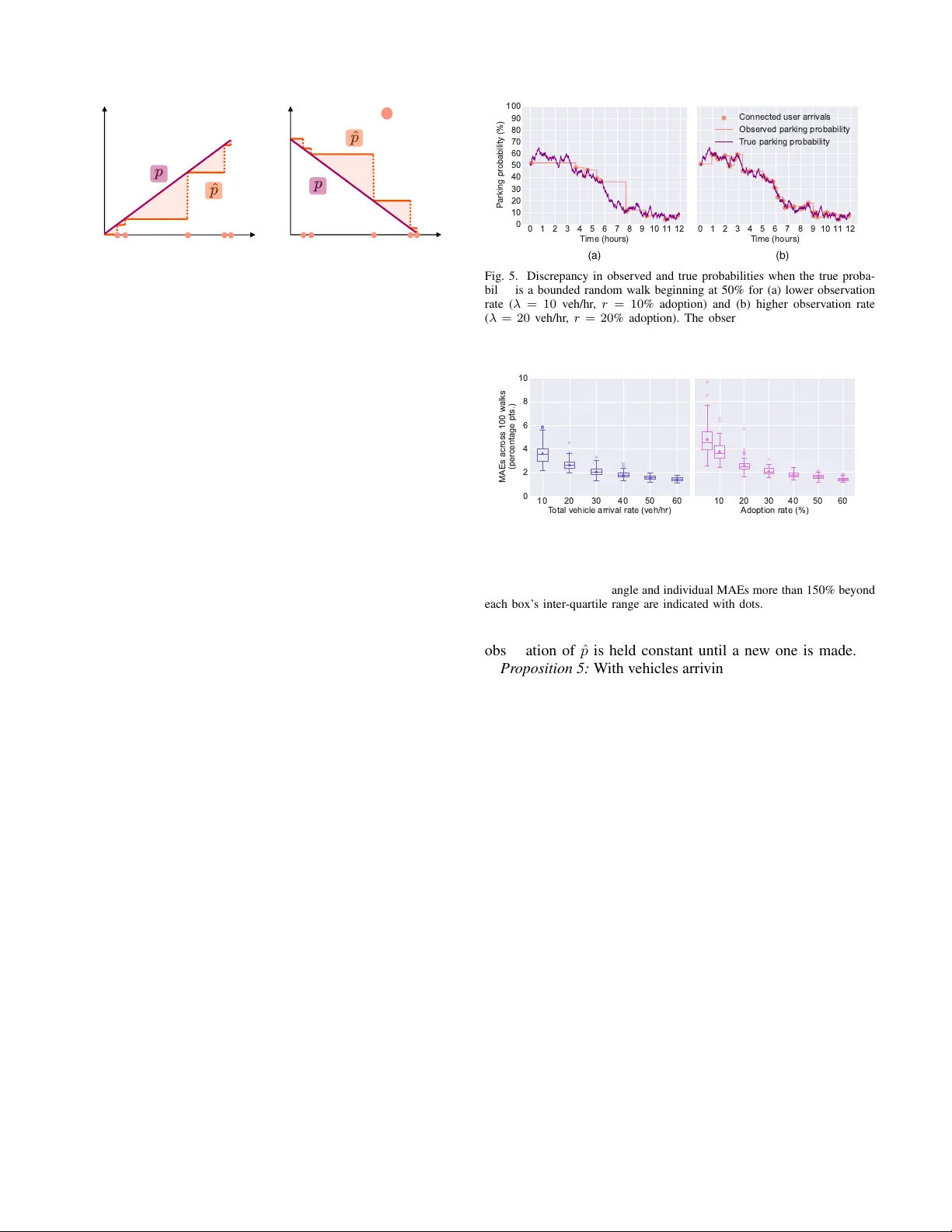
1 Probability-A ware P arking Selection Cameron Hickert, Member , IEEE, Sirui Li, Member , IEEE, Zhengbing He, Senior Member , IEEE, Cathy W u, Member , IEEE Abstract —Current navigation systems conflate time-to-drive with the true time-to-arrive by ignoring parking sear ch duration and the final walking leg. Such underestimation can significantly affect user experience, mode choice, congestion, and emissions. T o address this issue, this paper introduces the probability-aware parking selection problem, which aims to direct drivers to the best parking location rather than straight to their destination. An adaptable dynamic programming framework is proposed that leverages probabilistic, lot-level availability to minimize the expected time-to-arrive. Closed-form analysis determines when it is optimal to target a specific parking lot or explore alternatives, as well as the expected time cost. Sensitivity analysis and thr ee illustrative cases are examined, demonstrating the model’ s ability to account f or the dynamic nature of parking availability . Given the high cost of permanent sensing infrastructure, we assess the error rates of using stochastic observ ations to estimate av ailability . Experiments with real-world data fr om the US city of Seattle indicate this approach’ s viability, with mean absolute error decreasing from 7% to below 2% as observation frequency increases. In data-based simulations, probability-awar e strategies demonstrate time savings up to 66% relative to probability- unaware baselines, yet still take up to 123% longer than time- to-drive estimates. Index T erms —Parking, Navigation, Stochastic Modeling, Dy- namic Programming, T ravel Time. I . I N T R O D U C T I O N C URRENT navigation apps typically send driv ers to their destination, occasionally providing a basic assessment (e.g., ‘easy’, ‘difficult’) of parking in the area [1]. Gi ven that parking spaces may not exist at the destination or may be unav ailable, driv ers often need to find parking else where or cruise for parking at the current location until a spot becomes av ailable. For example, consider the parking garage at San Francisco General Hospital, located in an area with limited on-street parking: when it is full, dri ving to and walking from the next-closest garage adds at least 30 minutes for patients and visitors, according to Google Maps routing estimates. Similar scenarios, familiar to many urban driv ers and riders, highlight the frustrating difference between today’ s time-to- driv e estimates that ignore parking difficulties and more useful This work was supported in part by Cintra, the MIT Energy Initiative (MITEI), and the National Science Foundation (NSF) under grant numbers 2239566 and 2434399. Corresponding author s: Camer on Hickert, Zhengbing He Cameron Hickert and Sirui Li are with the Laboratory for Information & Decision Systems and the Institute for Data, Systems, and Society , Massachusetts Institute of T echnology , Cambridge, MA 02139, USA (Email: chickert@mit.edu; siruil@mit.edu ) Zhengbing He is with the Laboratory for Information & Decision Systems, Massachusetts Institute of T echnology , Cambridge, MA 02139, USA (Email: he.zb@hotmail.com ) Cathy W u is with the Laboratory for Information & Decision Systems, the Institute for Data, Systems, and Society , and the Dept. of Civil and En viron- mental Engineering, Massachusetts Institute of T echnology , Cambridge, MA 02139, USA (Email: cathywu@mit.edu ) T i m e - to - D ri v e ( S t a t u s Q u o ) T i me - to - A r ri v e : P a rk i n g P ro b a b i l i t y - U n a w a re T i m e - to - A r ri v e : P a rk i n g P ro b a b i l i t y - A w a re D r i v e T r a ve l Ti m e E s t im a t io n E r r o r Se a r c h W a l k T im e S a vi n g s R i d e P u b l i c T ra n si t T i m e - to - A r ri v e ( A p p s C o m p a r e w/ T im e - to - D r ive ) Fig. 1. Accounting for the search for parking and the post-parking walking leg can increase the accuracy of personal vehicle travel time estimates, sav e time, and improve cross-mode comparability . time-to-arriv e estimates that account for the parking search and post-parking walk time. See Figure 1. Beyond incon venience, underestimating the true time to arriv e via personal v ehicles may cause two other problems. First, it may prev ent mode shift that would occur if individuals had more accurate estimates [1]. This is particularly true giv en that popular navigation apps (e.g., Google Maps, Apple Maps) include estimates for w alking time from public transit to a final destination in their total public transit travel time estimates, but do not include walking time from av ailable parking to a final destination in their total dri ve time estimates [2]. Second, cruising for parking is known to contribute to congestion and emissions in urban environments [3]. T o address this issue, this paper introduces the probability- aware parking selection problem and proposes an adaptable dynamic programming framew ork to direct drivers to the best parking location based on location and parking lot-level probabilistic av ailability information, rather than directly to their destination. The dynamic programming framework offers a structured and adaptable theoretical foundation for closed- form analysis of optimal parking strategies under uncertainty , sensitivity , changing probabilities, as well as a mechanism for understanding trade-offs in volv ed. Results lev eraging real- world parking data from Seattle indicate stochastic obser- vations of true lot-le vel parking probabilities could be a viable estimation approach. In the analyzed cases, observed probabilities’ mean absolute error begins below 7% and falls below 2% as observations become more frequent. Simulations with real-world data across different settings demonstrate the practical potential of probability-aw are parking strategies. In all cases studied, these strategies outperform traditional meth- ods, achieving time savings of up to 66% in the setting with the highest congestion. The work makes four contributions: 2 • It establishes time-to-arriv e as a unified metric to enable fair comparison across transport modes, correcting the bias inherent in omitting search and walk times. • An introduction of the probability-aware parking selec- tion problem and a corresponding adaptable dynamic programming solution. • A closed-form analysis delineating when it is optimal to wait at a specific parking lot as opposed to when it may be better to visit other lots, as well as sensitivity analysis for dynamic probabilities. • A demonstration of the time savings from probability- aware parking strategies with stochastic observations. This includes a comparativ e case study using real-world parking data from Seattle that illustrates the utility of time-to-arriv e relativ e to time-to-driv e. This work is organized as follo ws: Section II revie ws the related literature. Section III introduces the dynamic pro- gramming problem and a corresponding solution, along with analysis for dynamic probability settings. Section IV details experiments that explore error from stochastic observations. Section V presents the Seattle case study. In Section VI the paper sets forth implications for future work. I I . R E L AT E D W O R K Probability-aware parking selection has ke y differences from the well-studied optimal stopping problem for park- ing [4]–[6], as well as other theoretical analyses of cruising [7]. Primarily , the driv er can decide where to go to seek parking, rather than passively waiting for av ailability to appear along a pre-defined route with strictly decreasing distance (usually) to the destination. Our analysis also considers probabilities at the lev el of entire parking lots rather than individual spaces, since the former is easier to estimate [8]. Still, our framework can accommodate spot-lev el analysis by treating each as its own individual lot. Even in optimal stopping v ariants that allo w backtracking, vehicles cannot alter the order of their visits to v arious spaces, the driving geometry is 1-dimensional, and parking av ailability odds rarely vary [6], [9]. T wo well-e xecuted closely related w orks are those described in [10] and [11]. Gi ven information about a driver’ s parking preferences, the road network, traffic rules, and parking reg- ulations, the algorithm in [10] greedily calculates expected driv er utility along possible routes to suggest a trajectory . [11] describes a routing approach based on the A* algorithm with a hand-designed cost function and focuses on the optimization of that function’ s weight term, which is specific to a giv en road network and set of static parking probabilities. Howe ver , these works consider only street parking, do not use closed- form analysis to express or compare possibilities, and focus on cruising within a predefined tolerance boundary of the final destination instead of a priori selection of parking destinations separate from the final destination. Furthermore, neither formulates a dynamic programming framework for the problem, addresses how parking information may be obtained, nor considers dynamic parking probabilities. V arious mobile applications e xist (e.g., SpotHero, SpotAn- gels, ParkCBR, Parking.com, Park Smarter) or have been proposed (e.g., ASPIRE [12]) for parking, but generally these are simple reserv ation and/or payment systems only for spots ov er which the app has control [13]. Other systems like iP arker address pricing, but not probability-based selection [14]. The surve y in [8] as well as the works in [15] and [16] in vestigate parking av ailability predictions. The present paper builds upon this research to better understand the utility of such enhanced parking estimates for users. [17] uses the possibility of time- and a vailability-a ware parking selection to motiv ate the work, b ut focuses on empirical probability prediction at specific lots with in-b uilt sensors in a vehicle’ s immediate vicinity . Still, our notion of parking probability aligns with theirs, i.e., the likelihood that at least one parking space is av ailable when a vehicle arriv es. I I I . M E T H O D O L O G Y A. F r amework The initial challenge is to construct a frame work capturing the spatial structure, time costs, information, and uncertainty in volv ed in parking while enabling closed-form analysis. W e model this situation using an infinite-horizon Markov decision process (MDP) M = ( S , A , P , R , s 0 ) ; see Figure 2. Each state s ∈ S is comprised of a tuple ( i, { u, o } ) where i ∈ { 0 , ..., N } index es the origin ( 0 ) and any of N on- or of f- street parking lots, and the set { u, o } indicates the vehicle’ s parking status, where u is u nparked and o is parked in an o pen spot. The initial state s 0 = (0 , u ) thus indicates an unparked vehicle at the origin. Parked states are terminal. At each timestep, let action a i ∈ A = { 1 , . . . , N } represent an attempt to park at lot i . Note that since there is no a 0 , a vehicle cannot attempt to stay at or return to the origin. This attempt succeeds with a lot-specific probability p i ∈ P and fails with probability 1 − p i . W e assume p i ∈ (0 , 1] . Let r i, ( j, { u,o } ) ∈ R represent the instantaneous reward incurred in the process of a vehicle beginning in state ( i, u ) and taking action a j to park in a dif ferent lot j . If this succeeds, it incurs rew ard r i, ( j,o ) = − t i → j − t j → D , where t i → j represents the drive time from i to j and t j → D represents the walk time from lot j to the true destination D . If the attempt fails, it only incurs drive time reward r i, ( j,u ) = − t i → j . If the vehicle remains unparked at any lot, it has tw o options for the follo wing timestep: either seek to park at a ne w lot k or else wait at the current lot for another chance at parking. The former incurs a reward of the formula just described, r j, ( k,u ) or r j, ( k,o ) . Let t wait indicate a wait time incurred for remaining at a lot and w aiting for another chance at parking. The latter incurs a reward r j, ( j,o ) = − t wait − t j → D if it successfully parks and r j, ( j,u ) = − t wait if it does not. In summary , the possible rew ards can be described: r i, ( j, status = { u,o } ) =          − t i → j − t j → D , if i  = j & status = o − t i → j , if i  = j & status = u − t wait − t j → D , if i = j & status = o − t wait , if i = j & status = u . This reward structure allows us to formally distinguish be- tween the con ventional time-to-drive metric and our proposed 3 Origin (1, u) Destination (implicit) (0, u) (1, o) a 1 → p 1 a 1 → 1 – p 1 r = - t 0 à 1 – t 1 à D r = - t 0 à 1 terminal r = 0 r = - t wait – t 1 à D a 1 → p 1 a 1 → 1 – p 1 r = - t wait (n, u) (n, o) a n → p n (n -1, u) (n -1, o) a 2 → p 2 . . a n → p n a n … a n → p n a n → 1 – p n a 2 → 1 – p 2 . . a n → 1 – p n a 1 . . a n - 1 a 1 . . a n - 1 D r = - t wait – t n à D Fig. 2. V isualization of the specified MDP . Orange states represent successful parking at the given lot ( · , o ) , and are terminal. Purple states represent those where the driver visits a lot, cannot immediately park, and thus must decide whether to visit another lot or wait at the current lot ( · , u ) . Actions ( a ) are shown with their associated probabilities ( p ), except where omitted for clarity of presentation. T o avoid over -complication, only select rew ards are shown; the full rew ard scheme is described in the main text. time-to-arrive metric. W e define the naive time-to-driv e esti- mate as the simple trav el time from origin to a target lot j , assuming immediate a vailability: t 0 → j . In contrast, we define time-to-arriv e as the magnitude of the cumulativ e reward collected over the entire trajectory τ until a terminal parked state is reached: − P h ∈ τ r h . Unlike time-to-dri ve, time-to- arriv e captures the stochastic components of the journey , including potential multiple driving legs ( t i → j ) and dwell times ( t wait ), as well as the final walking leg ( t j → D ). This distinction is critical for fair comparison across trans- portation modes. Current navigation platforms present time-to- driv e estimates alongside time-to-arriv e mass transit estimates that include wait and access/egress walk times. By omitting search and walking components, standard driving estimates present a structurally optimistic bias. Users, howe v er , may compare app-displayed values across modes as equiv alent estimates for total tra vel time. By e xplicitly modeling and opti- mizing for time-to-arrive, we correct this asymmetry , enabling valid cross-mode comparisons. The objectiv e is therefore to find the action sequence that minimizes expected time-to-arriv e (equiv alently , maximizes the expected sum of rewards). This framew ork excludes addi- tional driver preferences, such as pricing; future work could integrate these. The MDP can be seen as a stochastic shortest path problem in which the terminating goal states G ⊂ S are the parked states; this termination condition obviates the need for a discount factor γ in the framing. B. Optimal strate gy and cost with pr obabilistic information This work focuses on the case in which probabilistic parking av ailability information is accessible for each lot since it most closely relates to today’ s app-based driving decisions. Given pre-existing awareness of parking difficulty and app-generated data, it is uncommon to truly hav e no prior information about parking av ailability odds [1]. At the same time, real-time parking occupancy sensors are expensi ve and thus rare [10]. Our analysis finds the optimal strategy and associated time cost falls into two structure-based regimes, described in turn by the propositions below . Pr oposition 1: If, ∀ ( i, j ) pairs, t i → j ≥ t wait and t 0 → i = t 0 → j , then the optimal strategy is to dri ve directly to the lot i ∗ with the maximum value-to-go V i ∗ = − t i ∗ → D − 1 p i ∗ t wait . (1) Note that the decision to park at lot i can be conceptualized as a coin flip that succeeds (allo ws parking) with probability p i . t wait can be considered the time one must wait at a lot to again ‘flip the coin’ if the previous attempt was unsuccessful. Adopting a dynamic programming approach, one can thus explicitly write the cost for any ‘patient’ strategy , i.e., the strategy in which a vehicle driv es to the i th lot and waits there until it finds parking (possible since p i ∈ (0 , 1] ). The expected cumulativ e return E [ R i, patient ] of this strategy is written as E [ R i, patient ] = − t 0 → i − t i → D − X 1 ≤ m ≤∞ m · t wait · (1 − p i ) m − 1 p i , (2) where the sum corresponds to the expected value of a geomet- ric random variable with success probability p i . W e can thus rewrite the above as E [ R i, patient ] = − t 0 → i − t i → D − 1 p i t wait . (3) W e can write the v alue-to-go of any unparked state ( i, u ) under a patient policy at all times as V ( i,u ) , patient = − t i → D − 1 p i t wait . (4) By the second assumption in the proposition statement (namely , ∀ ( i, j ) pairs, t 0 → i = t 0 → j ), we have that i ∗ = arg max i ∈{ 0 ,...,N } V ( i,u ) , patient = arg max i ∈{ 0 ,...,N } E [ R i, patient ] . (5) 4 While this may seem a strong assumption, driv e times to parking lots near a destination of interest are often quite comparable, especially relative to driv e time variance due to other factors, e.g., traffic congestion, weather [18]. As an indication of this, empirical distributions of driv e times on urban roads have been sho wn to exhibit standard deviations one-third of their means [19]. Since we are concerned with a priori destination selection, this v ariance enhances the e xtent to which driv e times to two nearby locations may appear functionally similar , especially in comparison to the other time costs in volv ed, thus expanding the proposition’ s scope. The question now becomes whether one can do better than a patient strategy , i.e., by switching to a new lot j  = i ∗ in the case where parking in a chosen lot i ∗ is unsuccessful. Howe v er , note that this would incur the additional time cost of t i ∗ → j , which by assumption is at least as large as t wait . By this fact and by the assumption that t 0 → i ∗ = t 0 → j , we have − t 0 → i ∗ − t wait + V i ∗ , patient ≥ − t 0 → j − t wait + V j, patient ≥ − t 0 → i ∗ − t i ∗ → j + V j, patient , (6) where we also use the fact that V i ∗ , patient ≥ V j, patient , ∀ j due to the optimality of i ∗ . That is, any impatient strategy switching to a lot j and terminating at lot j will hav e a worse expected return than a patient strategy terminating at lot i ∗ . Therefore, in this regime, the optimal policy is a patient one in which the vehicle drives from the origin directly to lot i ∗ . Pr oposition 2: If ∃ t j → k < t wait , there may exist a cluster of parking lots { j, . . . , k } such that it is better to visit the lots in that cluster rather than adopt a patient strategy at a parking lot i with the single best v alue V ( i,u ) . Consider a cluster C of parking lots defined as those for which t i → j < t wait and t j → i < t wait . Following from the above analysis, we can write the expected cumulativ e return for the strategy in which a vehicle navigates to this cluster and cycles through those lots until parking is found as − t 0 →C − t C → D + 1 1 − Q i ∈C (1 − p i ) max {− t wait , − t C } , (7) where 1 − Q i ∈C (1 − p i ) is the probability that parking is av ailable at any lot i ∈ C ; t C represents the time to navigate among lots in that cluster; the max operator reflects our modeling assumption of the t wait waiting time between two consecutiv e ‘coin flips’ at the same lot; and t 0 →C , t C → D respectiv ely represent the trav el time from the origin to the cluster and from the cluster to the destination (both can be bounded above by taking their maximums among lots within the cluster). There are settings in which cycling through a cluster C of parking lots is better than the optimal single-lot patient strategy on lot i ∗ , ev en when lot i ∗ is not in the cluster C . These settings correspond to scenarios when (1) the joint probability 1 − Q i ∈C (1 − p i ) is high; (2) the travel time within the cluster t C is small; and (3) the travel time t 0 →C + t C → D is low . Intuiti vely speaking, these criteria reflect the fact that after an unsuccessful parking attempt at a lot i ∈ C , we can benefit from trying a different lot j ∈ C , j  = i during the wait for the next ‘coin flip’ at lot i , if we can tra vel from lot i to j relati vely quickly , and lot j has a relati vely high probability of parking. If the cluster C additionally incurs rel ativ ely lo w tra vel times with respect to the origin and destination, the cluster strategy could be better than the single-lot optimal patient strategy , where a time period of t wait would be wasted between each ‘coin flip’ at i ∗ . On the other hand, if these conditions are not satisfied, then the single-lot optimal patient strategy at i ∗ would remain optimal in the probabilistic availability information re gime. C. Sensitivity of the patient strate gy Pr oposition 3: If, ∀ ( i, j ) pairs, t i → j ≥ t wait and t 0 → i = t 0 → j , then the strategy of dri ving directly to lot i ∗ with the maximum v alue-to-go V i ∗ remains optimal so long as, ∀ j ∈ N ,  1 p j − 1 p i ∗  ≥ t 0 → i ∗ − t 0 → j + t i ∗ → D − t j → D . (8) This follows from the fact that the expected cumulativ e returns for i ∗ and j can be described as E [ R i ∗ , patient ] ≥ E [ R j, patient ] . Rewrit ing with Proposition 1 and rearranging, one arriv es at the result. Note the terms to the left of the “+” sign on the right-hand side of the inequality represent the dif ference in driv e times from the origin to lots i ∗ and j , while the terms to the right of that same “+” sign represent the difference in walk times from lots i ∗ and j to the destination. It is instructi v e to consider this in a decentralized, multi- agent context. If each of the vehicles in this setting has an optimal strategy as described above, that strategy remains optimal as long as the conditions described in Proposition 3 are maintained for that vehicle. Thus, the result is that no vehicle benefits by ‘defecting’ to another parking lot and a system-wide Nash equilibrium is maintained. Howe ver , if the conditions are not maintained, then the equilibrium may shift. D. Dynamic pr obabilities & thr ee illustrative cases Giv en the abov e sensitivity analysis, we now consider dynamic probabilities. In many settings, we do not expect walk time estimates between a parking lot and a destination of interest to vary considerably , and estimating driving time is a well-known feature of many of today’ s navigation apps as well as the subject of a number of pre vious works [20]–[22]. Con versely , the probability of parking at a specified lot may vary considerably throughout the day due to demand, duration of individual stays at a location, etc. W e inv estigate the impact of other vehicles in three settings that illustrate key mechanisms by which an ego vehicle’ s probability of parking can change. This in vestigation simul- taneously exhibits the dynamic programming frame work’ s ability to accommodate these analyses and to produce closed- form expressions for the resulting parking probabilities, which demonstrates how one could readily consider alternativ e situa- tions. W e consider three ‘orders’ of impact, shown in Figure 3 and described as follows: • First-order : Other vehicles attempt to park at the same lot as the ego vehicle. • Second-order : Other vehicles attempt to park at nearby lots, b ut resort to the ego vehicle’ s lot if parking at their first-choice lot is unav ailable. 5 1 … 1 2 n (a) First-order case 1 … 1 2 n 2 3 n (b) Second-order case 1 1 2 2 3 (c) Third-order case Fig. 3. V isualization of the three illustrativ e cases for dynamic probabilities. The ego vehicle is indicated with a star, the rectangles represent parking lots, and vehicles are arranged such that lower vehicles arrive earlier . • Third-order : Another vehicle does not attempt to park in the ego vehicle’ s lot, but affects the ego vehicle’ s parking probability via impacts on an interv ening parking lot. The cases are not intended to be exhausti ve; rather , they pro- vide insight into the mechanisms by which a vehicle’ s parking probability may vary as well as the associated mathematics. 1) F irst-or der case – arrivals to the same lot: Assume that n vehicles arrive to the same lot 1 as an ego vehicle within some near-term time t < t wait prior to that vehicle’ s arriv al. The probability for that lot p 1 thus becomes p ′ 1 , where p ′ 1 = p n 1 ; we can conceptualize it as multiple coin flips on the same ‘turn. ’ As the n th vehicle of this series to arri ve, the ego vehicle can only park if all the vehicles prior were able to park and there is space remaining. W e treat these as independent ev ents in this analysis, which is reasonable in large parking lots with suf ficient arri val and departure rates, when the time interval considered is appropriate, or when the true parking probability at a given lot is modeled as an underlying distribution. Howe v er , it may be a stronger assumption in other contexts. At first, it seems to fail to tak e advantage of additional information, namely , any vehicle which successfully parks prior to the ego vehicle ought to lower our estimate of the ego vehicle’ s ability to park. Howe v er , a successful parking ev ent provides informa- tion which can counteract this. For example, if a vehicle successfully parks, it may indicate timing is fav orable or that more vehicles are entering than exiting. Thus, it may not be appropriate to reduce a parking probability estimate for the ego vehicle conditional on a prior vehicle’ s successful parking ev ent. Additionally , the analysis and experiments further below consider the error incurred when we hav e access to only intermittent observations of a dynamic probability , such as can occur if arriving vehicles do affect the underlying probability . One interesting observation is that in the settings this work considers, the online setting is nearly equiv alent to the offline setting, and indeed entirely equiv alent if we allo w the online setting some ‘lookahead’ time. This is because other vehicles arriving to a lot after a vehicle is parked do not af fect that vehicle’ s odds of parking, and in the decentralized setting with self-interested agents there is no incentiv e to make suboptimal decisions in the short term to enhance parking options for vehicles yet to come. Furthermore, the lookahead time need only be as long as the time between the e go vehicle’ s departure and its parking, since the gap between useful online and of fline knowledge is simply the arri val of other vehicles to lots of interest in that period. This could be possible to some extent in settings where users were navigating to parking lots based on the recommendations from a navigation app. This lookahead time also presents a natural choice for the near-term time t < t wait mentioned above. 2) Second-or der case – arrivals to nearby lots: Consider when near-term prior arri vals occur at lots near the target lot for the ego vehicle (lot 1), but only proceed to that lot if parking at their ‘first-choice’ lot fails. This could occur for a variety of reasons, including if vehicles are pursuing the cluster-based strategy mentioned in Proposition 2. In this case, the updated probability for lot 1 becomes p ′ 1 = n Y j =1 p j + n X k =2 p k 1 (1 − p k ) n Y l = k +1 p l . (9) The proof follo ws from the fact that we can conceptualize of this as a series of coin flips, where the situation in which other vehicles attempt to park at lot 1 is a result of vehicles’ failures to park in other lots, and thus subject to those probabilities. One note: in the final element of Q n l = k +1 p l , k = n would mean that l > n , which would be beyond the allow able bounds for l . Thus, in this case, we simply set that term to 1. 3) Thir d-or der case – knock-on effects: Whereas Cases 1 and 2 consider n vehicles beyond the ego vehicle, for ease of exposition Case 3 only considers two other vehicles. More specifically , a third vehicle attempts to park at lot 3 prior to the others, but if it fails it will attempt to park at lot 2. That affects a second vehicle’ s ability to park at lot 2, which is its first-choice lot. If the second vehicle cannot park at lot 2, it will attempt to park at the ego vehicle’ s desired lot. In this way , the third vehicle affects the ego vehicle’ s ability to park despite never attempting to park in its lot. The proof follo ws directly from this logic. The updated probability p ′ 1 for the ego vehicle can be written as p ′ 1 = p 3 ( p 2 p 1 +(1 − p 2 ) p 2 1 ) + (1 − p 3 )[ p 1 p 2 2 + p 2 1 (1 − p 2 2 − (1 − p 2 ) 2 ) + (1 − p 2 ) 2 p 3 1 ] . (10) By way of interpretation, the p 1 p 2 2 term indicates the case in which both the second and third vehicles successfully park in lot 2. The p 2 1 indicates the case in which either the second or the third vehicle successfully parks in lot 2. The (1 − p 2 ) 2 term indicates the case in which neither of those vehicles is successful in parking in lot 2, and thus proceed to lot 1. 6 t (a) Linear increase = Poisson process arrivals t (b) Linear decrease Fig. 4. Error (shaded area) between an estimate ˆ p and the true value p when p is varying linearly and observation times are generated via a Poisson process. E. Err ors from stochastic pr obability observations If the underlying lot-level probabilities are dynamic, stochastic measurements will incur error as their recency fades. This can be an issue in light of the sensiti vity analysis abov e; i.e., if the observed probabilities deviate too much from the true probabilities, vehicles might route to suboptimal locations. Thus, we provide analysis and experiments belo w to inv es- tigate errors incurred when estimating dynamic probabilities via Poisson process-generated observations. Poisson processes are a well-kno wn stochastic modeling tool for random arriv al processes, including for parking analysis [23]–[27]. The analysis below applies to any pointwise-independent stochastic observation method and could easily be adapted to a variety of schemes. [8] provides a comprehensi ve surve y on parking prediction, particularly via data-dri ven methods for probability prediction. Near-term prediction is also discussed in [26]. For concreteness – and giv en the costs and effort associated with permanent infrastructure, continuous remote sensing, etc. – the current work considers that these Poisson observations are generated by connected users, where such users represent r fraction of the total population. This is inspired by the approach in [16]. For example, users of a given routing app or connected vehicles (autonomous or not) could provide insight into the a vailability at a lot to which the y arriv e or pass. [15] has illustrated the feasibility of a similar method, although that work le verages taxis and considers only on- street parking. Note, howe ver , that it would be straightforward to adapt the analysis to other Poisson stochastic observation methods, including schemes with remote sensing or paid staff, by adjusting the rate parameter . Pr oposition 4: W ith vehicles arri ving according to a Poisson process parameterized by arri val rate λ and connective tech- nology adoption rate r , the expected (mean) error between the true value of a variable p varying in a linear fashion with slope m and observ ations from connected users of that variable ˆ p will be m/λ 2 r 2 . This can be found by taking the e xpectation ov er the inte gral of a linear function with slope m (e.g., y = mx ) with respect to the integral’ s upper bound, where the upper bound is a random v ariable generated via a Poisson process with rate parameter λr . See Figure 4 for a visualization of the Poisson process-guided observation process, as well as the errors incurred. The result in Proposition 4 corresponds to the average size of the shaded regions in Figure 4. Each 0 1 2 3 4 5 6 7 8 9 10 1 1 12 T ime (hours) 0 10 20 30 40 50 60 70 80 90 100 Parking probability (%) (a) 0 1 2 3 4 5 6 7 8 9 10 1 1 12 T ime (hours) 0 10 20 30 40 50 60 70 80 90 100 Parking probability (%) Connected user arrivals Observed parking probability T rue parking probability (b) Fig. 5. Discrepancy in observed and true probabilities when the true proba- bility is a bounded random walk beginning at 50% for (a) lower observation rate ( λ = 10 veh/hr, r = 10 % adoption) and (b) higher observation rate ( λ = 20 veh/hr , r = 20 % adoption). The observation rate is a function of both the overall vehicle arrival rate λ and connected user adoption fraction r . 10 20 30 40 50 60 T otal vehicle arrival rate (veh/hr) 0 2 4 6 8 10 MAEs across 100 walks (percentage pts.) (a) 10 20 30 40 50 60 Adoption rate (%) 0 2 4 6 8 10 MAEs across 100 walks (percentage pts.) (b) Fig. 6. Distribution of mean absolute errors (MAEs) between observed and true probabilities across 100 different random walks as a function of (a) arriv al rates (with r = 20 %) and (b) adoption rates (with λ = 20 ). The distributional mean is indicated by a triangle and individual MAEs more than 150% beyond each box’ s inter-quartile range are indicated with dots. observation of ˆ p is held constant until a ne w one is made. Pr oposition 5: W ith vehicles arri ving according to a Poisson process parameterized by arri val rate λ and connective tech- nology adoption rate r , the expected (mean) error between the true value of a variable p increasing in an exponential fashion with exponent b and observations from connected users of that variable ˆ p will be b/ ( λr ) b +1 . As before, this can be found by taking the expectation ov er the integral of an exponential function with exponent b (e.g., y = x b ) with respect to the integral’ s upper bound, where the upper bound is a random variable generated via a Poisson process with rate parameter λr . Unlike before, the proof le verages the definition of the moments of an exponential distribution. This would correspond to the average size of the shaded regions in Figure 4 if the true probability function p were exponentially increasing. I V . N U M E R I C A L E X P E R I M E N T : S T O C H A S T I C O B S E RV A T I O N E R R O R The probabilities in the abov e analysis increased or de- creased monotonically . This may be rele vant in some settings, such as in the lead-up to or aftermath of a major e vent, or for commuter parking lots at the beginning and end of a workday . Obviously , these fail to characterize parking lots for which the dynamics are less predictable. T o accommodate this, we e valuate via simulation the er - rors incurred when making intermittent (Poisson process- generated) observations of a bounded random walk. The walk 7 P ike P la c e M a rke t C a rl S . E n g li s h J r . B o t a n ic a l G a rd e n Fig. 7. Locations of the destinations used in the Seattle case study . Base map sources: MapT iler, OpenStreetMap contributors. is bounded between 0% and 100% to mirror true probabilities and increments or decrements by one percentage point each minute. As before, observ ations are generated via a Poisson process with rate λr . Observ ations are again retained until a new one is made. Figure 5 provides a visualization of one such random walk under two separate observation rates. T o get a better sense of error, we also assess a verage error as a function of λ and r . Results are shown in Figure 6. These were generated by simulating the bounded random walks across 100 seeds at each arriv al or adoption rate. All began at a probability value of 50% and run for 12 hours of simulated time. Not only does the error decrease with more users, b ut in all settings studied, it remains relatively low , with mean absolute errors av eraging belo w 5%. For reference, with a drive, walk, and wait time of 15, 10, and 5 minutes respectively , a 5% overestimate of a 45% parking probability at a lot amounts to an expected travel time error in Equation 3 of less than one minute. Code and data for this pa- per are av ailable at https://github.com/chickert/ Probability- Aware- Parking- Selection . V . C A S E S T U DY : S E A T T L E PA R K I N G A. Pr obability observation err ors 1) Sites: T o validate the results of the proposed estimation approach across different times of day and urban parking settings, we introduce data provided by Seattle’ s Department of T ransportation (SDO T) [28], [29] for two separate areas: • (Dense) Area A.1 : 61 SDO T paid parking spots around the Pike Place Market (47.60943, -122.34183). • (Sparse) Area B.1 : 72 spots around the Carl S. English Jr . Botanical Garden (47.66687, -122.39747). They are selected to reflect heterogeneity: Area A.1 is a dense urban setting in the heart of downto wn Seattle with high traffic, while Area B.1 is located fiv e miles northwest and represents an area with lighter traf fic, less dense zoning, and sparser SDO T parking options. See Figure 7. 2) Scenario: W e use payment transactions collected on Thurs., Jan. 30th, 2025 as evidence of arriv als and take in verse occupancy rates as a proxy for parking probability . The data is av ailable for Area A.1 from 8am to 8pm and for Area B.1 from 8am to 6pm. Occupancy is computed from paid parking occupancy and the total parking space count. T o simulate connected users, we randomly sample the transaction data and assign the appropriate proportion as connected user arriv als. 8am 12pm 4pm 8pm T ime 0 20 40 60 80 100 Parking probability (%) Connected user arrivals Observed parking probability (a) 5 10 20 30 40 50 60 Adoption rate (%) 0 2 4 6 8 10 MAEs across 100 Seattle simulations (percentage pts.) Downtown Parking (Pike Place) Outskirts Parking (Botanical Garden) (b) Fig. 8. Dynamic probability results for two locations in Seattle: Pike Place Market (A.1, purple) and the Carl S. English Jr . Botanical Garden (B.1, teal). (a) Discrepancy in true and observed (orange) probabilities given the arriv als in SDOT data and a simulated 30 % connected user adoption rate. (b) MAE distributions as the adoption rate increases. Plot conv entions are as before. 3) Results: W e ev aluate stochastic probability observ ation via connected users by computing errors as in Section IV. Results are shown in Figure 8 with the same con ventions as in Figures 5 and 6. Giv en the connected user sampling inv olved, for the error box plots we again ev aluated 100 random seeds at each adoption rate. In all cases the mean and median MAE is below 7% and declines with increased adoption to belo w 2%. Interestingly , while Figure 8a sho ws the relative discrepancy between true and observed probabilities in Area B.1 to be greater than that at Area A.1 due to the lo wer effecti ve arriv al rate of connected users, Figure 8b indicates that – by the same token – the lo wer resulting volatility in Area B.1’ s parking probability produces MAEs that are more consistently low . B. Strate gy comparison T o v alidate the relativ e merits of probability-aware parking selection with stochastic observ ations, we conduct compar- isons against traditional (baseline) methods. This uses simu- lations of parking trials. 1) Sites: In this experiment, for each destination we now construct an MDP according to the framew ork in Section III, with N = 3 parking lots each. • (Dense) Area A.2 : Similar to Area A.1., Pike Place Market is the destination. The three lots, which comprise 98 spots, are those nearest the destination along Pike Place (Lot 1, closest), 2nd A venue (Lot 2, next closest), and Alaskan W ay (Lot 3, furthest). The origin is Kerry Park, a residential neighborhood chosen for its centrality within the city . Google Maps estimates an uncongested time-to-driv e of ten minutes and public transit total travel times (time-to-arrive) of 18-22 minutes, depending on the time of day . • (Sparse) Ar ea B.2 : The Botanical Garden is the desti- nation. The lots, which comprise 69 spots, include one on 54th St. (Lot 1) and the two nearest the Garden on Market St. (Lots 2 and 3, respectiv ely). Again, Lot 1 is the nearest to the destination and Lot 3 is furthest. The origin is Salmon Bay Park, selected to provide geographic heterogeneity as a residential hub in outer Seattle. Google Maps estimates an uncongested time-to- driv e of six minutes and public transit times of 21-23 minutes (again including walk time). 8 T ABLE I C O MPA R IS O N O F P RO B AB I L I TY -A W A RE S E LE C T I ON P O L IC I E S W I TH P A TI E N T A N D I M P A T I EN T B A S E LI N E S A C RO S S T E M PO R A L A N D S P ATI A L S E T TI N G S 10% Adoption Rate 50% Adoption Rate Destination Day Policy Mean T ime ± Std. ( ↓ ) Gain vs. BL-Pat. ( ↑ ) Gain vs. BL-Imp. ( ↑ ) Perf. vs. Oracle ( ↑ ) Mean T ime ± Std. ( ↓ ) Gain vs. BL-Pat. ( ↑ ) Gain vs. BL-Imp. ( ↑ ) Perf. vs. Oracle ( ↑ ) Area A.2 (Pike Place Market) W eek- day BL-Patient 44.6 ± 20.1 — — — 45.2 ± 19.4 — — — BL-Impat. 21.9 ± 5.6 50.9% — — 20.8 ± 6.3 54.0% — — P A 1-Step 20.0 ± 7.4 55.2% 8.7% -8.2% 19.6 ± 4.1 56.8% 6.1% -1.3% P A 2-Step 19.6 ± 4.7 55.9% 10.2% -1.8% 21.4 ± 6.8 52.6% -2.9% 2.1% P A 3-Step 19.0 ± 4.3 57.4% 13.2% 0.5% 19.1 ± 5.2 57.7% 8.1% -7.2% W eek- end BL-Patient 55.6 ± 13.2 — — — 56.2 ± 12.4 — — — BL-Impat. 27.3 ± 9.9 50.9% — — 25.3 ± 7.9 55.1% — — P A 1-Step 21.9 ± 9.1 60.7% 20.0% -5.4% 19.7 ± 4.2 65.0% 22.1% 5.0% P A 2-Step 22.3 ± 9.4 59.9% 18.4% -15.3% 19.1 ± 3.8 66.1% 24.5% -3.4% P A 3-Step 22.4 ± 9.0 59.7% 18.1% -12.6% 19.8 ± 4.6 64.8% 21.7% 11.9% Area B.2 (Botanical Garden) W eek- day BL-Patient 10.3 ± 1.2 — — — 10.2 ± 1.0 — — — BL-Impat. 10.8 ± 2.2 -4.4% — — 10.5 ± 1.9 -2.8% — — P A 1-Step 10.0 ± 0.0 3.2% 7.2% 1.1% 10.1 ± 0.7 1.1% 3.8% 1.1% P A 2-Step 10.8 ± 3.1 -4.4% 0.0% -4.4% 10.1 ± 0.7 1.1% 3.8% 1.1% P A 3-Step 10.2 ± 1.0 1.1% 5.2% 0.0% 10.1 ± 0.7 1.1% 3.8% -1.1% W eek- end BL-Patient 14.6 ± 8.4 — — — 14.0 ± 8.9 — — — BL-Impat. 13.8 ± 5.2 5.1% — — 14.0 ± 5.5 -0.1% — — P A 1-Step 13.4 ± 4.5 8.1% 3.2% 1.1% 11.6 ± 2.4 17.1% 17.3% 5.5% P A 2-Step 13.5 ± 3.6 7.3% 2.4% 1.3% 13.4 ± 3.4 4.4% 4.6% -5.1% P A 3-Step 13.8 ± 5.5 5.1% 0.0% -8.3% 13.6 ± 5.4 3.0% 3.1% -9.7% For brevity , ‘P A ’ indicates probability-aware policies and ‘BL ’ indicates baselines. Up arrows indicate that higher values are preferable for the metric, while down arrows indicate the opposite. Times are reported in minutes. Boldface denotes the top performance within each adoption rate category . See the main text for further details. Darker shading indicates larger performance differences. All parking lots were selected as viable options (i.e., within a 10-minute w alk from their destination) with dif fering parking av ailabilities. Origins are picked such that the driv e times to each lot are approximately equal. 2) Scenarios: T o capture temporal heterogeneity , we simu- late multiple days and departure times. The weekday selected is Thurs., Jan. 30th, 2025, and the weekend day selected is Sat., Feb . 1st, 2025. The selection of this weekend date for Area A.2 is intentional to consider e vent interference: a festiv al brought crowds to the area for music, art, and shopping. For each day we simulate trips beginning each hour from 8am to 6pm for Area A.2 and from 8am to 4pm for Area B.2 (since SDO T parking data collection stops earlier for these lots). Connected user arri vals and observ ations are modeled as in Section V -A. Results are reported for 10% and 50% user adoption rates to explore the impact of errors on system reliability , but were similar for other values. F or rob ustness giv en the stochastic nature of the simulations, we run each simulation for fiv e random seeds at each departure time across the locations, dates, and adoption rates. Driv e times and walk times are estimates from Google Maps. W e set t wait = 5 minutes. The true parking probabilities at each of the six lots are extracted from SDO T data as described in Section V -A. 3) P olicies: W e design three probability-aw are (P A) park- ing selection policies and two baseline methods against which to v alidate their relative merits. Dynamic probabilities preclude the possibility of computing the true value of each possible action. W e do not assume future probabilities at each lot are known. The ev aluated policies are: • P A 1-Step computes a probability risk-adjusted time cost heuristic c i,j = ( t i → j /p j ) + t j → D for each lot j from the current lot i (including the possibility that i = j ), then attempts to park in the lot with the lo west projected cost. Note this is a ‘one-step’ heuristic in that it only considers the odds of parking at the target lot. • P A 2-Step ‘looks ahead’ to consider the option(s) av ail- able should the immediate parking attempt fail. It is thus recursiv e. The two-step cost heuristic may be written c i,j = t i → j + p j ( t j → D ) + (1 − p j )(min i ∈{ 0 ,...,N } c j,i ) ; note this last term is the cost heuristic for the best possible action if the first parking attempt fails. • P A 3-Step is a three-step heuristic that extends the consideration one step further and follows the same mathematical structure. Note that we still do not assume access to future probability knowledge. Thus, while each additional step incorporates more knowledge about the system’ s current state, this may introduce error in a dynamic setting such as ours. Greedy patient and impatient policies serve as baselines. These are derived from the recommendations of popular navigation apps and how users may behav e in response, either by waiting or seeking additional nearby parking [1]. • Baseline-Patient is a patient strategy that finds the lot closest to the destination and waits there until parked. • Baseline-Impatient is an impatient policy that first at- tempts to park at the lot closest to the destination. If this fails, it dri ves to the un visited lot closest to its current position to continue its search. If all lots hav e been visited, the search cycle resets. Since the patient policy may produce unrealistically long waits during low-a vailability times, we cap this policy’ s search at 1 hour to prevent skewed results. 9 4) Results: For each simulation we compute the time-to- arriv e. This is the per-episode cumulativ e rew ard, as described in Section III-A. The results from these experiments are shown in terms of time savings and loss in T able I. The means and standard deviations (in minutes) of trip durations are presented for each setting. Gains are computed as percent improv ements over the baseline policies’ mean times. Policies in bold indicate a top performance in either the 10% or the 50% adoption rate category . T o better understand the causes of errors and their impacts on the system, we also compare probability-aware policies against oracle baselines that ha ve access to the current true parking probabilities at each lot, rather than those generated from connected user observ ations. These quantify the effect of suboptimal probability awareness. The results indicate probability-aware parking selection strategies, even with probability estimates generated stochas- tically via connected users, outperform more traditional meth- ods. Improvements reach up to 66% relativ e to the patient baseline and 24% relativ e to the impatient baseline. As hy- pothesized, these gains are greater when parking is scarce: the weekend at Area A.2 is the busiest setting, while the the weekday at Area B.2 has the least traffic. The findings are notable in comparison to each location’ s time-to-driv e. See T able II. Even for the best probability-aware policies across all scenarios studied, the average time-to-arriv e is 67% to 123% higher than the time-to-driv e directly to the destinations. This discrepanc y is up to 462% and 173% for the patient and impatient baselines, respectiv ely . This shows how tra vel time projections that do not account for parking can substantially underestimate the true v alue. This difference may be rele v ant for users deciding which mode to take. In the case of the route from Kerry Park to Pike Place Market (A.2), the public transit time-to-arriv e estimates are substantially shorter than the mean time-to-arri ve values of the baseline driving strate gies and similar to the values from the best probability-aware driving strategies; see T able III. In contrast, the time-to-drive projection is 50% shorter than the average public transit time-to-arri ve. This could mean that users may mistakenly disregard public transit because they believ e it requires double the time of driving a personal vehicle, when the opposite may be true (or the options may at least be similar). Note that uncongested drive time estimates were used for conserv atism – we expect increased traf fic w ould tend to add more time to the parking strategies than the direct driv e time, since they generally comprise longer distances. 5) Err or impact: Interestingly , performance is comparable across the two adoption rates. This suggests limited operational impact from errors incurred via stochastic observ ation. The probability-aware policies’ performance relativ e to their ora- cles also supports this conclusion, although those at the 50% adoption rate perform slightly better relativ e to their oracles than those at the 10% rate. One explanation for the system’ s resilience to errors may be the following trade-off: probability estimates (and by extension, errors) may matter more in com- petitiv e settings, but competitiv e parking en vironments also hav e higher traf fic, which produces more frequent observ ations of a lot’ s parking a vailability . The results across the 1-, 2-, and 3-step lookahead probability-aw are policies suggest that T ABLE II T I ME - T O - A R R IV E V S . T I M E - T O -D R I V E : A B S . & P C T . D I FF E RE N C E S ( ↓ ) 10% Adoption 50% Adoption Dest. Day Policy Minutes % Minutes % Area A.2 (Pike Place) W eek- day BL-Pat. 34.6 346% 35.2 352% BL-Imp. 11.9 119% 10.8 108% Best P A 9.0 90% 9.1 91% W eek- end BL-Pat. 45.6 456% 46.2 462% BL-Imp. 17.3 173% 15.3 153% Best P A 11.9 119% 9.1 91% Area B.2 (Bot. Gdn.) W eek- day BL-Pat. 4.3 72% 4.2 70% BL-Imp. 4.8 80% 4.5 75% Best P A 4.0 67% 4.1 68% W eek- end BL-Pat. 8.6 143% 8.0 133% BL-Imp. 7.8 130% 8.0 133% Best P A 7.4 123% 5.6 93% V alues represent the absolute gap and percentage increase of time-to-arrive over time-to-dri ve. Each policy’ s time-to-arrive is the mean recorded in T able I. ‘Best P A ’ refers to the probability-aware policy with the lowest mean time for a given scenario. Each destination’ s time-to-driv e is as described in Section V -B.1. Lo wer is better . Darker shading indicates more severe time- to-driv e underestimates relativ e to time-to-arrive. T ABLE III D R IV I N G T I ME - T O - A R R IV E V S . P U B L IC T R AN S I T T I M E - T O - A R R IV E F O R A R EA A . 2 ( P IK E P L AC E M A R K ET ) : A B S . & P C T . D I FF E RE N C E S 10% Adoption 50% Adoption Day Policy Minutes % Minutes % W eekday BL-Patient 24.6 123% 25.2 126% BL-Impat. 1.9 10% 0.8 4% Best P A -1.0 -5% -0.9 -4% W eekend BL-Patient 35.6 178% 36.2 181% BL-Impat. 7.3 37% 5.3 27% Best P A 1.9 10% -0.9 -4% V alues represent the difference in time-to-arriv e for driving relativ e to public transit. Each dri ving polic y’ s time-to-arri ve is defined as in T able II. The public transit time-to-arrive estimate used is 20 minutes, the midpoint of the range described in the Section V -B.1 site description for Area A.2. For reference, this site’ s time-to- drive estimate is 10 minutes shorter (-50%) than the estimated public transit time-to-arrive. Dark er shading indicates larger deviations. Purple is used since larger values are not necessarily worse – more accurate total trav el time estimates enable fairer cross-mode comparison. deeper lookaheads – which incur computational complexity exponential in the depth of the search – may not be necessary . V I . F U T U R E W O R K Future work could find analytical expressions for alter- nativ e cases or explore uncertainty in dri ve and walk time estimates. Large-scale e xperiments assessing the advantages and disadvantages of the strategies outlined abov e would be welcome, as would identification of parking clusters C and in vestigation of additional probability-aware strategies, perhaps with reinforcement learning. Related work could be done to estimate the reduction in carbon emissions and time sav ed via mode shift if time-to-dri ve estimates are corrected to time-to-arri ve estimates. These could also integrate driv er preference models that consider factors beyond travel time. 10 R E F E R E N C E S [1] N. Arora, J. Cook, R. Kumar , I. Kuznetsov , Y . Li, H.-J. Liang, A. Miller, A. T omkins, I. Tsogsuren, and Y . W ang, “Hard to park? Estimating parking difficulty at scale, ” in Pr oceedings of the 25th ACM SIGKDD International Confer ence on Knowledge Discovery & Data Mining , 2019, pp. 2296–2304. [2] Y . Y in, “Private communication during conference in emerging tech- nologies in transportation systems (TRC-30), ” 2024. [3] D. C. Shoup, “Cruising for parking, ” T ransport policy , vol. 13, no. 6, pp. 479–486, 2006. [4] M. Sakaguchi and M. T amaki, “On the optimal parking problem in which spaces appear randomly , ” 1982. [5] M. T amaki, “ An optimal parking problem, ” Journal of Applied Pr oba- bility , pp. 803–814, 1982. [6] ——, “Optimal stopping in the parking problem with U-turn, ” Journal of applied pr obability , vol. 25, no. 2, pp. 363–374, 1988. [7] R. Arnott and P . W illiams, “Cruising for parking around a circle, ” T ransportation r esearc h part B: methodological , vol. 104, pp. 357–375, 2017. [8] X. Xiao, Z. Peng, Y . Lin, Z. Jin, W . Shao, R. Chen, N. Cheng, and G. Mao, “Parking prediction in smart cities: A survey , ” IEEE T ransactions on Intelligent T ransportation Systems , vol. 24, no. 10, pp. 10 302–10 326, 2023. [9] P . Krapivsk y and S. Redner, “Simple parking strategies, ” J ournal of Statistical Mechanics: Theory and Experiment , vol. 2019, no. 9, p. 093404, 2019. [10] N. Djuric, M. Grbovic, and S. V ucetic, “Parkassistant: An algorithm for guiding a car to a parking spot, ” in T ransportation Researc h Board 95th Annual Meeting , vol. 16, 2016, p. 5433. [11] M. Hedderich, U. Fastenrath, and K. Bogenberger, “Optimization of a park spot route based on the A* algorithm, ” in 2018 21st International Confer ence on Intelligent T ransportation Systems (ITSC) . IEEE, 2018, pp. 3493–3498. [12] S. R. Rizvi, S. Zehra, and S. Olariu, “ Aspire: An agent-oriented smart parking recommendation system for smart cities, ” IEEE Intelligent T ransportation Systems Magazine , vol. 11, no. 4, pp. 48–61, 2018. [13] D. T eodorovi ´ c and P . Lu ˇ ci ´ c, “Intelligent parking systems, ” European Journal of Operational Research , vol. 175, no. 3, pp. 1666–1681, 2006. [14] A. O. Kotb, Y .-C. Shen, X. Zhu, and Y . Huang, “iParker—A new smart car-parking system based on dynamic resource allocation and pricing, ” IEEE transactions on intelligent transportation systems , vol. 17, no. 9, pp. 2637–2647, 2016. [15] F . Bock, S. Di Martino, and A. Origlia, “Smart parking: Using a crowd of taxis to sense on-street parking space availability , ” IEEE T ransactions on Intelligent Tr ansportation Systems , vol. 21, no. 2, pp. 496–508, 2019. [16] F . Shi, D. W u, D. I. Arkhipov , Q. Liu, A. C. Regan, and J. A. McCann, “Parkcro wd: Reliable crowdsensing for aggregation and dissemination of parking space information, ” IEEE T ransactions on Intelligent T rans- portation Systems , vol. 20, no. 11, pp. 4032–4044, 2018. [17] E. H.-K. W u, J. Sahoo, C.-Y . Liu, M.-H. Jin, and S.-H. Lin, “ Agile urban parking recommendation service for intelligent vehicular guiding system, ” IEEE Intelligent Tr ansportation Systems Magazine , vol. 6, no. 1, pp. 35–49, 2014. [18] S. Peer, C. C. K oopmans, and E. T . V erhoef, “Prediction of travel time variability for cost-benefit analysis, ” T r ansportation Research P art A: P olicy and Practice , vol. 46, no. 1, pp. 79–90, 2012. [19] M. Fosgerau and D. Fukuda, “V aluing travel time variability: Character- istics of the trav el time distribution on an urban road, ” T ransportation Resear ch P art C: Emerging T ec hnologies , vol. 24, pp. 83–101, 2012. [20] D. Bertsimas, A. Delarue, P . Jaillet, and S. Martin, “Tra vel time estimation in the age of big data, ” Operations Research , vol. 67, no. 2, pp. 498–515, 2019. [21] K. Uchida, “Estimating the value of travel time and of tra vel time reliability in road networks, ” Tr ansportation Resear ch P art B: Method- ological , vol. 66, pp. 129–147, 2014. [22] D. W ang, J. Zhang, W . Cao, J. Li, and Y . Zheng, “When will you arrive? Estimating trav el time based on deep neural networks, ” in Proceedings of the AAAI confer ence on artificial intelligence , vol. 32, no. 1, 2018. [23] G. F . Newell, Applications of Queueing Theory . Springer, 1982. [24] J. A. Lav al, Z. He, and F . Castrillon, “Stochastic extension of Newell’ s three-detector method, ” T r ansportation Researc h Recor d , vol. 2315, no. 1, pp. 73–80, 2012. [25] Y . A. Kutoyants, Introduction to the Statistics of P oisson Processes and Applications . Springer Nature, 2023. [26] J. Xiao, Y . Lou, and J. Frisby , “How likely am I to find parking? – A practical model-based framew ork for predicting parking availability , ” T ransportation Researc h P art B: Methodological , vol. 112, pp. 19–39, 2018. [27] A. Ogulenko, I. Benenson, and N. Fulman, “The nature of the on-street parking search, ” T ransportation Researc h P art B: Methodological , vol. 166, pp. 48–68, 2022. [28] S. D. of Transportation (SDOT), “Paid parking occupancy - Last 30 days, ” 2025. [Online]. A v ailable: https://data.seattle.gov/T ransportation/ Paid- Parking- Occupanc y- Last- 30- Days- /rke9- rsvs/about data [29] ——, “Paid parking transaction data, ” 2025. [Online]. A v ailable: https://data.seattle.gov/T ransportation/Paid- P arking- Transaction- Data/ gg89- k5p6/about data Cameron Hickert earned a B.S. in physics from the Univ ersity of Denver and an M.E. in computational science and engineering from Harvard University . He is currently a Ph.D. student in Social and En- gineering Systems at MIT . His research interests include safe autonomy , reinforcement learning, and distributed cyber-physical systems. Sirui Li received her B.S. degree with majors in computer science and mathematics from W ashington Univ ersity in St. Louis, MO, USA, in 2019. She is currently working toward her Ph.D. degree in Social and Engineering Systems at MIT , Cambridge, MA, USA. Her research interests include areas of machine learning for combinatorial optimization and control analysis for transportation systems. Zhengbing He (M’17-SM’20) receiv ed the Bache- lor of Arts degree in English language and litera- ture from Dalian Univ ersity of Foreign Languages, China, in 2006, and the Ph.D. degree in systems engineering from Tianjin University , China, in 2011. He was a Post-Doctoral Researcher and an Assistant Professor with Beijing Jiaotong University , China. From 2018 to 2022, he was a Full Professor with Beijing University of T echnology , China. Presently , he is a Research Scientist at MIT . His research stands at the intersection of trans- portation, systems engineering, and artificial intelligence. He has published more than 180 papers, with total citations exceeding 7,000. He is the Editor- in-Chief of Journal of T ransportation Engineering and Information (Chinese). Meanwhile, he serves as a Senior Editor for IEEE TRANSA CTIONS ON INTELLIGENT TRANSPORT A TION SYSTEMS, an Associate Editor for IEEE TRANSACTIONS ON INTELLIGENT VEHICLES, and an Editorial Advisory Board Member for Transportation Research Part C. His webpage is https://www .GoT raf ficGo.com. Cathy W u (Member , IEEE) receiv ed B.S. and M.Eng. degrees from MIT and a Ph.D. degree from UC Berkeley , all in EECS. She was a post-doctoral researcher at Microsoft Research. She is currently the Class of 1954 Career De velopment Associate Professor at MIT in LIDS, CEE, and IDSS. She studies machine learning for optimization, with a focus on urban mobility . She is interested in enabli ng faster , evidence-dri ven decisions for sociotechnical systems. Cathy is the recipient of the NSF CAREER (2023), the Ole Madsen Mentoring A ward (2025), the IEEE ITS Best Dissertation A ward (2019), and the CUTC Milton Pikarsky Memorial A ward (2018). She serves on the Board of Governors for the IEEE ITSS, is an Associate Editor or Area Chair for ICML, NeurIPS, ICRA, and T ransportation Research Part C, and served as Program Co-chair for RLC 2025. She is also the inaugural Chair and Co-founder of the REproducible Research In T ransportation Engineering (RERITE) W orking Group.